aeroelastic response of bird-damaged fan blades using a

Aeroelastic Response of Bird-Damaged Fan Blades

Using a Coupled CFD/CSD Framework

Eric R. Muir∗ and Peretz P. Friedmann†

Department of Aerospace Engineering, The University of Michigan, Ann Arbor, MI, 48109, USA

The aeroelastic response of a bird-damaged fan stage at the inlet of a high-bypass ratioturbofan engine is examined using a combined CFD/CSD model. ANSYS CFX is usedfor the computational fluid dynamic (CFD) calculations combined with the ANSYS Multi-field (MFX) solver that couples ANSYS CFX with ANSYS Mechanical APDL to performaeroelastic response calculations. The damaged fan sector consists of 5 blades that repre-sent the geometry resulting from a numerical bird strike simulation. The forced responseof the undamaged blades downstream of the damaged sector exhibits the highest level ofstructural response. The structural response of these undamaged blades is dominated bythe first bending mode and increases in amplitude with time. The aeroelastic responseshows a similar behavior, with the downstream undamaged blades exhibiting a growingstructural response that is dominated by the first bending mode. The aeroelastic responseof the damaged blades also contains contributions from the second torsion mode. An ex-amination of the work exerted by the aerodynamic forces suggests that the growth in bladeresponse for the upstream damaged blade is due to an aeroelastic behavior that may beindicative of a potential instability.

Nomenclature

D Number of RBF driver points

m Mass flow rate

mR Referred mass flow rate

qm Generalized degree of freedom of the mth mode

p Aerodynamic static pressure

P Aerodynamic total pressure

PR Total pressure ratio

R Blade tip radius

S CFD element surface area

t Time

T Aerodynamic total temperature

Uθ Angular deformation (cylindrical coordinates)

WAR Aerodynamic work calculated from aeroelastic calculations

WFR Aerodynamic work calculated from forced response calculations

aΩ Assembled centrifugal acceleration vector

C RBF interpolant coefficient vector

Faero Assembled aerodynamic force vector

FΩ Assembled centrifugal force vector

K Assembled FEM stiffness matrix

∗Ph. D. Candidate, Student Member AIAA.†Francois-Xavier Bagnound Professor of Aerospace Engineering, Fellow AIAA and AHS.

1 of 24

American Institute of Aeronautics and Astronautics

Dow

nloa

ded

by U

nive

rsity

of

Mic

higa

n -

Dud

erst

adt C

ente

r on

Dec

embe

r 13

, 201

7 | h

ttp://

arc.

aiaa

.org

| D

OI:

10.

2514

/6.2

014-

0334

55th AIAA/ASME/ASCE/AHS/ASC Structures, Structural Dynamics, and Materials Conference

13-17 January 2014, National Harbor, Maryland

10.2514/6.2014-0334

Copyright © 2014 by E.

R. Muir and P. P. Friedmann. Published by the American Institute of Aeronautics and Astronautics, Inc., with permission.

AIAA SciTech Forum

http://crossmark.crossref.org/dialog/?doi=10.2514%2F6.2014-0334&domain=pdf&date_stamp=2014-01-10

M Assembled FEM mass matrix

n Element normal vector

Qj Aerodynamic force vector on j-th node of CFD mesh

r Radius vector

U Assembled nodal deformation vector

x = (x, y, z) Nodal position vector

xd = x, y, zT RBF driver point

xe = x, y, zT RBF evaluation point

Coordinate Systems

< r, θ, z > Global cylindrical coordinate system

< x, y, z > Global Cartesian coordinate system

Greek Symbols

α HHT-α time-integration parameter

β HHT-α time-integration parameter

γ HHT-α time-integration parameter

ε FSI load transfer convergence tolerance

τ Aerodynamic viscous wall shear stress

φ Radial basis function

Γ CFD mesh diffusivity

Λ CFD element volume

Λref Reference CFD element volume

Ω Engine rotation speed

δ CFD mesh displacement

ς CFD mesh deformation vector

ς RBF interpolant of the CFD mesh deformation

ϕ FSI interface load/displacement vector

Φm Mode shape deformation of the mth mode

Ω = 0, 0,ΩT Engine rotation vector

Subscripts

m Mode number

STD Standard atmosphere conditions

Superscript

j Reference to node j in the CFD mesh˙( )=d⁄dt Differentiation with time

Abbreviations

1B First bending mode

2B Second bending mode

1T First torsion mode

3B Third bending mode

2T Second torsion mode

CAD Computer Aided Design

CFD Computational Fluid Dynamics

CSD Computational Structural Dynamics

2 of 24


Dow

nloa

ded

by U

nive

rsity

of

Mic

higa

n -

Dud

erst

adt C

ente

r on

Dec

embe

r 13

, 201

7 | h

ttp://

arc.

aiaa

.org

| D

OI:

10.

2514

/6.2

014-

0334

FEM Finite Element Method

FSI Fluid Structure Interface

RANS Reynolds-averaged Navier-Stokes

RBF Radial basis function

RBFN Radial basis function network

I. Introduction, Background, and Objectives

Bird strike on jet engine fan blades is important for the design of both civilian and military aircraft.Bird strikes occur primarily during takeoff and landing due to the tendency of birds to congregate in the

vicinity of the ground.1 The low altitude at which bird strikes occur limits recovery options and enhances therisk due to bird strike. The turbofan engines used in commercial and military aircraft have a large intake areacovered by fan blades that increases the chance of bird strikes. Furthermore, the thin, low aspect ratio, lowcamber fan blades used in modern turbofans are structurally and aerodynamically optimized for efficiencyat normal operating conditions, and bird damage induces off-design operation.2 Therefore, turbofan designsrepresent a sophisticated trade-off between structural integrity, propulsive efficiency, and robustness underbird strike.

During bird-strike, the bird hits the fan blades, fragments, and propagates through the engine core andbypass duct. The impact can cause substantial deformation of the blade leading edge combined with bendingand twist of the blade.3 It can also induce crack propagation and fatigue failure.3 Furthermore, the structuraldynamics and unsteady aerodynamic loading caused by bird damage induce a complex aeroelastic responseproblem that can lead to aeroelastic instability.4,5 Predicting the aeroelastic behavior of a bird damagedfan blade represents a significant design barrier in the development of improved-efficiency turbofan engines.

The Federal Aviation Administration (FAA) mandates comprehensive standards for bird strike resis-tance.6 These standards require that each engine maintain 75% of the maximum rated thrust and meetengine handling requirements for a series of post bird strike operating conditions that simulate an emergencylanding sequence. Successful demonstration of compliance with Federal Aviation Regulations (FAR) Part 33in which a bird is fired with an air cannon at a test stand mounted, running engine is required for certifica-tion. Several complete-engine tests are required to demonstrate compliance with these regulations, and eachtest destroys a new engine. Therefore, the cost associated with engine certification for bird-strike is high.

Complete-engine tests are infeasible within the design iteration process due to the associated cost. As aresult, approximate component-based engine tests are performed to isolate the bird damage by firing a birdat a subset of the engine (typically the fan stage) that is rotated in a vacuum.1,3, 7 Such tests determine theability of the fan blades to retain their structural integrity during and after a bird strike event. The damagedfan stage is then installed in an otherwise undamaged engine to assess the effect of the bird-damaged fanblades on the engine aerodynamic performance and aeroelastic response. Experimental tests demonstratethat bird damage may reduce flutter margins and produce rotating stall, reinforcing the importance of anaccurate bird-strike aeroelastic analysis.8

Numerical simulations provide a cost effective means for assessing the aerodynamic loading and aeroe-lastic behavior of a damaged fan. However, the combined aerodynamic and structural dynamic modelingof a bird-damaged fan assembly, where the damage is typically isolated to a sector of blades, is a complexproblem. The structural model must accommodate the asymmetry caused by the bird-damaged fan bladesand the aerodynamic model must be time-accurate, nonlinear, viscous, and include a turbulence modelto address time-dependent flow separation and reattachment.9 Computational structural dynamics (CSD)based on the finite element method (FEM) are typically used to model the bird impact and resulting struc-tural response since it can represent complex material behavior and non-linear geometric deformations.10–16

Computational fluid dynamics (CFD) is required to accurately capture the complex flow phenomena associ-ated with bird damaged turbofans.17,18 Reliable CSD and CFD methods exist to compute the bird impact,structural dynamic response, and unsteady aerodynamic loads of a damaged fan blade. However, due to thecomputational times required for CFD methods, the structural and aerodynamic computations are typicallyperformed separately in an uncoupled or loosely coupled manner. Therefore, the aeroelastic effects may beinaccurate.

Despite its importance, only a limited number of computational studies have considered the aeroelasticresponse of a bird-damaged fan. In a unique set of studies, Imregun et al.8,9 examined the aeroelasticstability of a bird-damaged fan using a fully coupled CFD/CSD formulation in the time domain in which

3 of 24


Dow

nloa

ded

by U

nive

rsity

of

Mic

higa

n -

Dud

erst

adt C

ente

r on

Dec

embe

r 13

, 201

7 | h

ttp://

arc.

aiaa

.org

| D

OI:

10.

2514

/6.2

014-

0334

the form of the bird-damage is “assumed” and isolated to two blades. In Ref. 9, the fully coupled analysisdemonstrates instability of the first torsion mode of a damaged blade; however, it is unclear if the growth inmodal displacement is the result of a flutter mechanism or the strong wake shed by the upstream damagedblade. In Ref. 8, the aeroelastic response was also found to be sensitive to flight conditions, with fluttermargins reduced at low pressure ratios and rotating stall occurring at high pressure ratios. Rotating stall isa well-known unsteady flow phenomena in axial compressors in which an upstream flow disturbance causesa sector of the fan blades to stall, typically at the blade tip. The stalled blades result in pockets of stagnantair, denoted stall cells, that rotate circumferentially at the blade tips producing large, unsteady aerodynamicloads on the blades.

These studies provide insight into the aerodynamic behavior and aeroelastic response of a bird-damagedfan. However, the damage considered in Refs. 8 and 9 was not representative of realistic blade damagedue to bird-strike certification tests, where leading edge damage over a large region of the blade span isaccompanied by global bending and twist of the blade. Also, the turbofan geometries in these studies didnot resemble modern, high-bypass turbofans and the damaged sector is limited to two blades. Furthermore,the aeroelastic response calculations of Refs. 8 and 9 were performed at 70% engine rotational speed, whilebird-strike typically occurs during take-off at 100% engine rotation speed.

For improved understanding of the bird-strike problem, a computational aeroelastic study of a bird dam-aged commercial turbofan operating at take-off conditions is needed, where the bird damage is representativeof experimental bird strike tests or accurate numerical simulation of the bird-strike event. In Ref. 19, theauthors presented an aerodynamic model suitable for use in an aeroelastic study of a bird-damaged commer-cial turbofan engine together with the steady-state and unsteady flow field resulting from the bird-damagedfan. Subsequently in Ref. 20, the aerodynamic model and a structural dynamic model were combined andforced response calculations were performed to gain insight into this complex system behavior. The currentstudy extends the forced response framework to accommodate two-way coupling between the aerodynamicand structural dynamic models of the bird damaged fan and aeroelastic response calculations are performed.The overall objective of this paper is to compare the blade response resulting from one-way forced responseand fully-coupled aeroelastic response calculations and thus assess the role of complete aeroelastic couplingon the response. The specific objectives of this study are:

1. Describe a coupled CFD/CSD framework that is suitable for a fully-coupled aeroelastic stability andresponse calculation of bird damaged turbofans.

2. Describe the steady and unsteady flow associated with a fan sector consisting of five bird-damagedblades that are representative of a practical bird-strike configuration.

3. Study in detail the forced response and aeroelastic response of a bird-damaged fan stage under postbird-strike conditions.

4. Compare the aerodynamic work calculated from the forced response and aeroelastic response calcula-tions to identify the potential for aeroelastic instability.

II. Fan Blade Geometry

The turbofan geometry examined is representative of a commercial, high-bypass ratio turbofan. Theaerodynamic geometry of each fan blade is described by a set of constant-span cross-sections referred toas blade profiles, as shown in Fig. 1(a). The structural geometry is described by a computer aided design(CAD) model of the fan blade, as shown in Fig. 1(b), defined by the aerodynamic blade profiles.

LS-DYNA is employed to numerically simulate the bird strike problem and obtain the bird-damagedconfiguration. The LS-DYNA code is a general purpose FEM program that has been used extensively tomodel bird-strike problems, and it has proven itself to be a reliable tool for modeling blade damage.10 Thesimulated bird-strike event mimics a typical bird-strike experimental test sequence in vacuum: spin the fanstage at a specified engine rotational speed, fire a bird at the fan stage, continue to spin the engine untilthe transient response of the blades subsides, slow the fan stage to zero engine rotational speed. In thisprocess, the rotating fan stage is referred to as “hot” and differs from the non-rotating “cold” fan stage dueto centrifugal effects. Furthermore, the fan stage before the bird-strike is referred to as “undamaged” whereas the fan stage after the bird-strike is referred to as “damaged”.

4 of 24


Dow

nloa

ded

by U

nive

rsity

of

Mic

higa

n -

Dud

erst

adt C

ente

r on

Dec

embe

r 13

, 201

7 | h

ttp://

arc.

aiaa

.org

| D

OI:

10.

2514

/6.2

014-

0334

(a) Aerodynamicblade profiles.

Blade Prole

(b) Undamagedblade.

Blade Prole

(c) Damaged blade. (d) Bird-damaged fan.

Figure 1: Aerodynamic blade profiles and the CAD model of the damaged fan.

The damaged geometry considered is due to a single 2.5 pound (lb) bird ingested at take-off conditionsat a strike location of 70% blade span. The bird strike involves a subset of 5 blades, and the remainingblades are undamaged. The blade damage is interpolated to generate the damaged blade profiles that definethe aerodynamic and CAD-based structural geometries of the bird-damaged fan blades. Figure 1(c) depictsthe CAD model of a damaged blade defined by the aerodynamic blade profiles. Figure 1(d) shows the CADmodel of the full, damaged fan, where the damaged blades are highlighted in orange and the blades arenumbered.

III. Aerodynamic Model

The ANSYS CFX commercial aerodynamic solver is used to model the compressible unsteady flow gov-erned by the Reynolds-averaged Navier Stokes (RANS) equations. ANSYS CFX utilizes a finite volumeapproach that yields a near second-order accurate spatial discretization. A second-order accurate backwardEuler time-integration scheme is used for the unsteady calculations. The k-ε turbulence model is employedand scalable wall functions are used to resolve the near-wall boundary layer. The fluid is assumed to be idealand calorically perfect.

A. Computational Domain

The CFD calculation is restricted to an isolated fan stage suitable for prediction of the performance char-acteristics and unsteady aerodynamic behavior of a bird-damaged fan. The fan stage starts downstream ofthe engine inlet, extends into the bypass duct and core duct, and includes a set of fan blades, a rotatinghub, a stationary shroud, and a stationary splitter, illustrated by Fig. 2. The hub, shroud, and splittergeometries are defined by two-dimensional curves in the r-z plane, and the three-dimension hub, shroud,and splitter surfaces are obtained by full revolution of these curves about the engine centerline. The surfacesconnecting the edges of the hub, shroud, and splitter define the inflow, bypass duct outflow, and core ductoutflow boundaries of the computational domain. A clearance between the blade tip and shroud is specifiedto accurately account for the influence of the tip gap on flow losses and shock structure.

B. Computational Mesh

ANSYS TurboGrid is utilized to generate a high-quality, structured CFD mesh of hexahedral elements for anundamaged single blade passage. ANSYS TurboGrid cannot accommodate geometries with a splitter thatbisects the domain outflow. Instead, ANSYS Meshing is used to create an unstructured hexahedral meshfor the outlet. Conventional mesh topologies, such as H-Grid, J-Grid, C-Grid, L-grid, and O-grid, requirea substantial amount of user manipulation to construct a CFD mesh of acceptable quality, particularly forcomplex blade geometries. Furthermore, these conventional topologies often result in an overly fine meshwithin the blade passage to ensure a sufficient boundary layer resolution. ANSYS TurboGrid contains an

5 of 24


Dow

nloa

ded

by U

nive

rsity

of

Mic

higa

n -

Dud

erst

adt C

ente

r on

Dec

embe

r 13

, 201

7 | h

ttp://

arc.

aiaa

.org

| D

OI:

10.

2514

/6.2

014-

0334

Bypa

ss D

uct O

uto

wCo

re D

uct

Out

ow

Rotating Hub

Stationary Shroud

Ino

w

Splitter

zr

Blade Prole

Figure 2: Meridional cross-section of the fan stage computational domain.

Automatic Topology and Meshing (ATM) optimized topology method that is used to create high-quality,structured meshes of an undamaged fan without the constraints of conventional topologies.

The mesh topology, mesh density, and boundary layer resolution for the undamaged CFD mesh aredetermined by the physical flow phenomena anticipated and the degree of accuracy desired from the CFDsolution. Proper resolution of the boundary layer and tip gap is essential to capture the shock structure andflow losses due to viscosity in the boundary layer and flow leakage through the tip gap. Mesh sensitivitystudies were conducted in Ref. 19, and it was concluded that the “coarse” mesh identified in Ref. 19 issufficiently accurate for the objectives of the current study. A constant-span cross-section at 75% blade spanis shown in Fig. 3(a), and an overall meridional view of the computational mesh of the coarse mesh for asingle blade passage is depict in Fig. 3(b). The mesh consists of 10.4 million nodes and 9.7 million elements.

(a) CFD mesh at 75% blade span. (b) Meridional view of CFD mesh.

Figure 3: Constant-span and meridional cross-sections of the CFD mesh.

The ANSYS TurboGrid ATM topology is not applicable for full wheel geometries that include a set ofdamaged blades. To extend the high mesh quality produced by the ANSYS Turbo Grid ATM mesh topologyto the damaged fan geometry, the automated mesh deformation scheme presented in Ref. 19 is utilized.This procedure employs a radial basis function network (RBFN) to interpolate the deformation from thebird damaged blades to the CFD mesh of the undamaged wheel. RBFN interpolation is an effective tool

6 of 24


Dow

nloa

ded

by U

nive

rsity

of

Mic

higa

n -

Dud

erst

adt C

ente

r on

Dec

embe

r 13

, 201

7 | h

ttp://

arc.

aiaa

.org

| D

OI:

10.

2514

/6.2

014-

0334

for multivariate interpolation and has been successfully utilized for large-amplitude mesh deformation inaeroelastic applications and CFD-based aerodynamic shape optimization studies.21–26

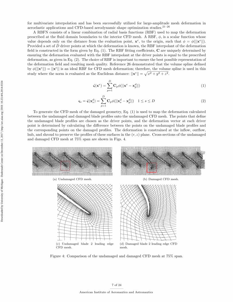
A RBFN consists of a linear combination of radial basis functions (RBF) used to map the deformationprescribed at the fluid domain boundaries to the interior CFD mesh. A RBF, φ, is a scalar function whosevalue depends only on the distance from the evaluation point, xe, to the origin, such that φ = φ(||xe||).Provided a set of D driver points at which the deformation is known, the RBF interpolant of the deformationfield is constructed in the form given by Eq. (1). The RBF fitting coefficients, C are uniquely determined byensuring the deformation evaluated with the RBF interpolant at the driver points is equal to the prescribeddeformation, as given in Eq. (2). The choice of RBF is important to ensure the best possible representation ofthe deformation field and resulting mesh quality. Reference 26 demonstrated that the volume spline definedby φ(||xe||) = ||xe|| is an ideal RBF for CFD mesh deformation; therefore, the volume spline is used in this

study where the norm is evaluated as the Euclidean distance: ||xe|| =√x2 + y2 + z2.

ς(xe) =D∑

p=1

Cpφ(||xe − xdp||) (1)

ςs = ς(xds) =D∑

p=1

Cpφ(||xds − xdp||) 1 ≤ s ≤ D (2)

To generate the CFD mesh of the damaged geometry, Eq. (1) is used to map the deformation calculatedbetween the undamaged and damaged blade profiles onto the undamaged CFD mesh. The points that definethe undamaged blade profiles are chosen as the driver points, and the deformation vector at each driverpoint is determined by calculating the difference between the points on the undamaged blade profiles andthe corresponding points on the damaged profiles. The deformation is constrained at the inflow, outflow,hub, and shroud to preserve the profiles of these surfaces in the (r, z) plane. Cross-sections of the undamagedand damaged CFD mesh at 75% span are shown in Figs. 4.

(a) Undamaged CFD mesh. (b) Damaged CFD mesh.

(c) Undamaged blade 2 leading edgeCFD mesh.

(d) Damaged blade 2 leading edge CFDmesh.

Figure 4: Comparison of the undamaged and damaged CFD mesh at 75% span.

7 of 24


Dow

nloa

ded

by U

nive

rsity

of

Mic

higa

n -

Dud

erst

adt C

ente

r on

Dec

embe

r 13

, 201

7 | h

ttp://

arc.

aiaa

.org

| D

OI:

10.

2514

/6.2

014-

0334

C. Boundary Conditions

At the domain inflow, the total pressure, total temperature, turbulence intensity, and flow direction of theincoming flow that correspond to a particular flight condition are enforced. The total pressure distributionincludes flow losses due to the upstream engine inlet nacelle. At the core duct outflow, the mass flow rate isspecified with the assumption that the engine core “pulls” a fixed mass flow rate through the core duct fora given operating condition (free-stream condition and engine rotation speed). Static pressure is enforced atthe bypass duct outflow using a radial-equilibrium condition that permits the static pressure to vary radiallywhile maintaining the specified static pressure on average. Solid wall boundary conditions are enforced atthe fan blades, hub, shroud, and splitter such that the velocity of the flow matches that of the wall throughspecification of a no-slip condition. A zero wall velocity is prescribed at the shroud and splitter, and anon-zero wall velocity that results from engine rotation is prescribed at the blades and hub.

D. Operating Condition

The performance of a fan stage is characterized by the total pressure ratio and referred mass flow rate.The total pressure ratio is defined as the ratio of the mass flow averaged total pressure at the bypass ductoutflow to the mass flow averaged total pressure just upstream of the fan blades. The referred mass flow rate,calculated using Eq. (3), is the mass flow rate through the domain corrected for non-standard day inflowconditions and represents the mass flow that would pass through the fan if the inflow total pressure andtotal temperature corresponded to standard day conditions. The operating point of a fan stage is describedby the total pressure ratio and referred mass flow rate resulting from operation at a particular operatingcondition defined by the engine rotation speed, inflow conditions, and outflow static pressure. The inflowtotal pressure and total temperature correspond to free-stream conditions, and the outflow static pressurerepresents the back-pressure produced by downstream engine components.

mR = m

√T

TSTD

(PSTDP

)(3)

A fan map depicts the operating points obtained using numerical simulations and experimental testsof an isolated fan stage for a variety of operating conditions. The operating points obtained with variousoutflow static pressures at a fixed engine speed and inflow conditions are connected to form characteristiccurves. The stall point is identified by the peak in total pressure ratio along a characteristic curve andindicates the onset of stall. Stall is an undesirable, unsteady flow phenomena produced by flow separationthat typically occurs at low mass flow rates and high bypass duct static pressure. A stall line connects thestall points on each characteristic curve and identifies the boundary of steady flow, where operating pointsto the left of the stall line are unsteady. A fan map also includes the fan operating line that consists of theunique set of operating points produced by the fan stage when installed in a complete engine. The operatingline is measured during an infinitesimally slow throttle sweep of a complete-engine operating at a particularfree-stream condition. A representative fan map that includes several characteristic curves, the associatedstall points, and the stall line is shown in Fig. 5.

For proper representation of the fan operating in a complete engine using a CFD model of an isolatedfan stage, a bypass duct static pressure boundary condition is specified so that the predicted operating pointcoincides with a point on the operating line. The bypass duct static pressure necessary to achieve the desiredoperating point at the intersection of the characteristic curve and the operating line is unknown a priori.Therefore, an iterative procedure is utilized to map the characteristic curve and determine the bypass ductstatic pressure that yields an operating point within 1% error of the operating line. The error is calculatedusing Eq. (4) where the predicted operating point is denoted by

(m

R, PR

), and ∆mR and ∆PR denote the

horizontal and vertical distance of the operating point from the operating line, as shown in Fig. 5.

%∆OL =

√(∆mR

mR

)2

+

(∆PR

PR

)2

× 100 (4)

IV. Structural Dynamic Model

The structural dynamic model is implemented using ANSYS Mechanical APDL, a commercial FEM-based structural dynamics solver. The computational domain for the structural dynamic model consists of

8 of 24


Dow

nloa

ded

by U

nive

rsity

of

Mic

higa

n -

Dud

erst

adt C

ente

r on

Dec

embe

r 13

, 201

7 | h

ttp://

arc.

aiaa

.org

| D

OI:

10.

2514

/6.2

014-

0334

Referred Mass Flow

Pres

sure

Rat

io

mR, PR

)ΔmR

ΔPR

Ω3

Ω2Ω1

Operating LineStall LineCharacteristic CurveStall PointPredicted Operating Point

Unsteady FlowSteady Flow

Desired Operating Point

Increasing Static Pressure

Figure 5: Representative fan map.

24 individual blades each cantilevered at the blade root. The hub disk is not modeled since its flexibility isassumed to be insignificant compared to that of the fan blades. The fan blade material is titanium and ismodeled with a linearly elastic material law.

A. Computational Mesh

The structural mesh follows a structured topology such that the structural elements on the wetted surfaceof the blade completely overlap with the CFD mesh at the blade surface. The structural mesh also featuresa curved leading edge and trailing edge to aid in load and displacement transfer between the structuraland aerodynamic meshes. The fan blades are modeled using 8-noded, solid, hexahedral elements (ANSYSSOLID185 element type) with three translational degrees of freedom at each node. A mesh sensitivity wasconducted to identify the mesh resolution suitable for the objections of this study. The structural meshutilized in this study consists of 5712 nodes and 4020 elements per blade for a total of 137,088 nodes and96,480 elements. Figure 6(a) shows the structural mesh of an undamaged blade. Figure 6(b) shows thecomputational mesh of the damaged fan, where the damaged blades are highlighted in orange.

(a) Structural meshfor an undamagedblade.

(b) Bird-damaged structural mesh with damagedblades highlighted in orange.

Figure 6: Structural mesh for the damaged fan.

9 of 24


Dow

nloa

ded

by U

nive

rsity

of

Mic

higa

n -

Dud

erst

adt C

ente

r on

Dec

embe

r 13

, 201

7 | h

ttp://

arc.

aiaa

.org

| D

OI:

10.

2514

/6.2

014-

0334

B. Rotating Mode Shapes

The first 5 mode shapes of a rotating, undamaged fan blade at take-off engine rotational speed are shownin Figs. 7. The natural frequencies of the first 5 mode shapes are listed in Table 2. The mode shapes of thedamaged blades are similar to those of the undamaged blade, and the rotating natural frequencies for eachdamaged blade are provided in Table 2.

(a) 1st bending. (b) 2nd bending. (c) 1st torsion. (d) 3rd bending. (e) 2nd torsion.

Figure 7: First 5 mode shapes of a rotating, undamaged blade.

Table 2: Natural frequencies of the first 5 modes of the rotating undamaged and damaged blades.

1st Bending 2nd Bending 1st Torsion 3rd Bending 2nd Torsion

(1B) (2B) (1T) (3B) (2T)

Undamaged 126.97 Hz 262.95 Hz 381.21 Hz 532.65 Hz 712.65 Hz

Blade 1 126.98 Hz 263.61 Hz 373.44 Hz 537.52 Hz 699.62 Hz





C. Equations of Motion

The equations of motion solved by ANSYS Mechanical APDL are derived from the principle of virtual work.The mass and stiffness matrices are assembled for the entire structural mesh using standard methods, andthe assembled deformation vector, U, contains the translational degrees of freedom for each node. The finalequation of motion is given by Eq. (5), where FΩ accounts for the centrifugal effects due to engine rotation.The assembled force vector, Faero represents the aerodynamic force transferred from the CFD mesh to thestructural mesh.

MU + K(U)U = FΩ + Faero (5)

The structural dynamic model includes a large deflection formulation to accommodate changes in thestiffness matrix that result from structural deformation. Therefore, the equations of motion represent anonlinear set of equations where the stiffness matrix is a function of the deformation vector, K = f(U). ANewton-Raphson iterative procedure is implemented to update the stiffness matrix within each time-step.A description of the Newton-Raphson algorithm that is utilized by ANSYS Mechanical APDL is providedin the ANSYS Mechanical APDL Theory Reference Guide.27

The HHT-α time-integration scheme is used to solve Eq. (5) in time. The HHT-α is an extensionof the Newmark time-integration method that damps out spurious high-frequency response by introducingcontrollable numerical dissipation in higher frequency modes while maintaining second-order accuracy.28 TheHHT-α is unconditionally stable and second-order accurate if the parameters meet the criteria described byEqs. (6)-(8). For this study, the ANSYS default values for the HHT-α formulation are used: γ = 0.6,

10 of 24


Dow

nloa

ded

by U

nive

rsity

of

Mic

higa

n -

Dud

erst

adt C

ente

r on

Dec

embe

r 13

, 201

7 | h

ttp://

arc.

aiaa

.org

| D

OI:

10.

2514

/6.2

014-

0334

β = 0.3025, and α = 0.1. Further details on the HHT-α scheme and its implementation are provided in theANSYS Mechanical APDL Theory Reference Guide.27

γ = 1/2 + α (6)

β = (1 + α)2/4 (7)

0 ≤ α ≤ 1/3 (8)

V. Coupled Fluid-Structure Framework

The ANSYS Multi-field solver is used to couple the ANSYS CFX aerodynamic solver and ANSYS Me-chanical APDL structural solver. The computational frameworks and coupling algorithm for the one-wayand fully-coupled fluid-structure interaction calculations are provided next. Further information is availablein the ANSYS documentation.29

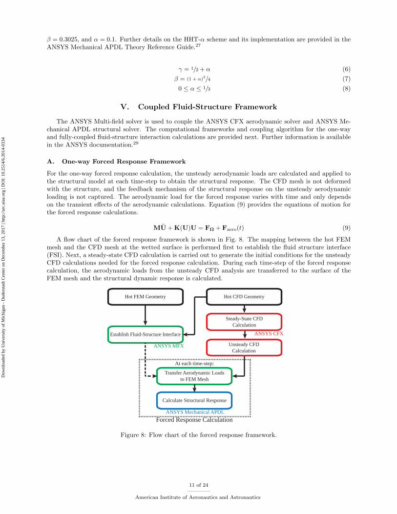
A. One-way Forced Response Framework

For the one-way forced response calculation, the unsteady aerodynamic loads are calculated and applied tothe structural model at each time-step to obtain the structural response. The CFD mesh is not deformedwith the structure, and the feedback mechanism of the structural response on the unsteady aerodynamicloading is not captured. The aerodynamic load for the forced response varies with time and only dependson the transient effects of the aerodynamic calculations. Equation (9) provides the equations of motion forthe forced response calculations.

MU + K(U)U = FΩ + Faero(t) (9)

A flow chart of the forced response framework is shown in Fig. 8. The mapping between the hot FEMmesh and the CFD mesh at the wetted surface is performed first to establish the fluid structure interface(FSI). Next, a steady-state CFD calculation is carried out to generate the initial conditions for the unsteadyCFD calculations needed for the forced response calculation. During each time-step of the forced responsecalculation, the aerodynamic loads from the unsteady CFD analysis are transferred to the surface of theFEM mesh and the structural dynamic response is calculated.

Hot CFD Geometry

Establish Fluid-Structure Interface

Unsteady CFDCalculation

Calculate Structural Response

Transfer Aerodynamic Loadsto FEM Mesh

Hot FEM Geometry

ANSYS Mechanical APDL

ANSYS CFX

ANSYS MFX

Forced Response Calculation

Steady-State CFDCalculation

At each time-step:

Figure 8: Flow chart of the forced response framework.

11 of 24


Dow

nloa

ded

by U

nive

rsity

of

Mic

higa

n -

Dud

erst

adt C

ente

r on

Dec

embe

r 13

, 201

7 | h

ttp://

arc.

aiaa

.org

| D

OI:

10.

2514

/6.2

014-

0334

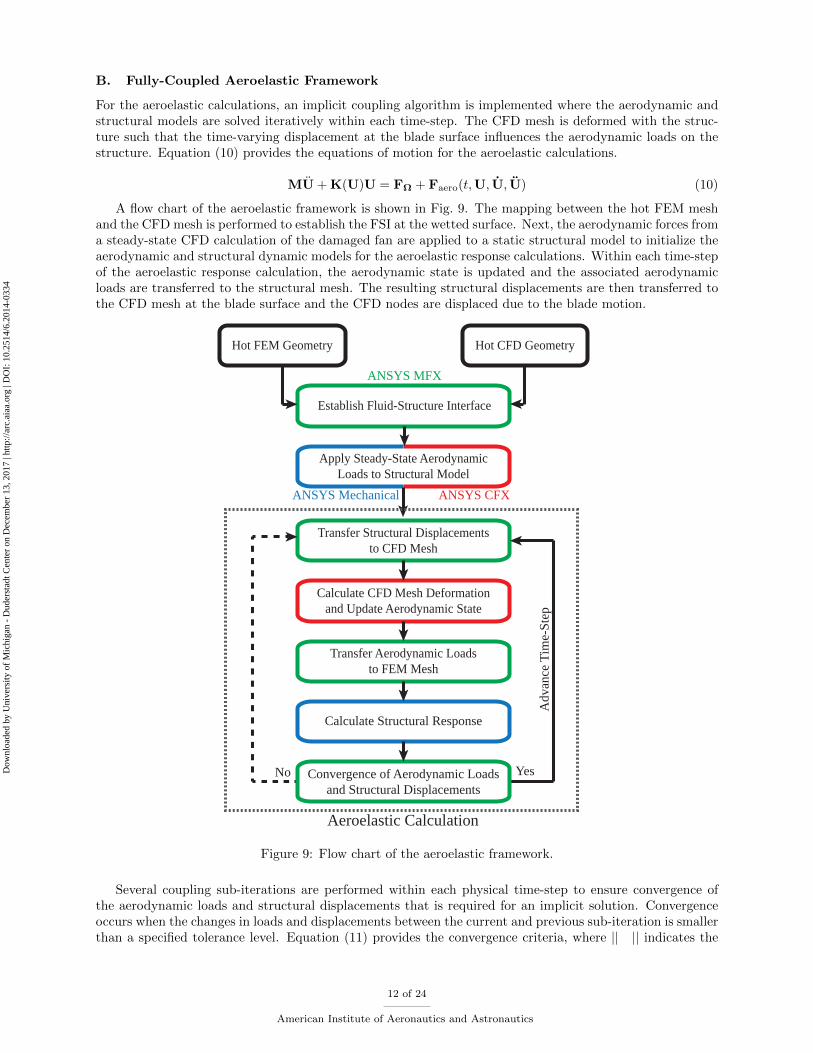
B. Fully-Coupled Aeroelastic Framework

For the aeroelastic calculations, an implicit coupling algorithm is implemented where the aerodynamic andstructural models are solved iteratively within each time-step. The CFD mesh is deformed with the struc-ture such that the time-varying displacement at the blade surface influences the aerodynamic loads on thestructure. Equation (10) provides the equations of motion for the aeroelastic calculations.

MU + K(U)U = FΩ + Faero(t,U, U, U) (10)

A flow chart of the aeroelastic framework is shown in Fig. 9. The mapping between the hot FEM meshand the CFD mesh is performed to establish the FSI at the wetted surface. Next, the aerodynamic forces froma steady-state CFD calculation of the damaged fan are applied to a static structural model to initialize theaerodynamic and structural dynamic models for the aeroelastic response calculations. Within each time-stepof the aeroelastic response calculation, the aerodynamic state is updated and the associated aerodynamicloads are transferred to the structural mesh. The resulting structural displacements are then transferred tothe CFD mesh at the blade surface and the CFD nodes are displaced due to the blade motion.

Hot CFD Geometry

Establish Fluid-Structure Interface

Apply Steady-State AerodynamicLoads to Structural Model

Adv

ance

Tim

e-St

ep

Calculate CFD Mesh Deformationand Update Aerodynamic State

Calculate Structural Response

Transfer Structural Displacementsto CFD Mesh

Transfer Aerodynamic Loadsto FEM Mesh

No YesConvergence of Aerodynamic Loadsand Structural Displacements

Hot FEM Geometry

ANSYS Mechanical ANSYS CFX

ANSYS MFX

Aeroelastic Calculation

Figure 9: Flow chart of the aeroelastic framework.

Several coupling sub-iterations are performed within each physical time-step to ensure convergence ofthe aerodynamic loads and structural displacements that is required for an implicit solution. Convergenceoccurs when the changes in loads and displacements between the current and previous sub-iteration is smallerthan a specified tolerance level. Equation (11) provides the convergence criteria, where || || indicates the

12 of 24


Dow

nloa

ded

by U

nive

rsity

of

Mic

higa

n -

Dud

erst

adt C

ente

r on

Dec

embe

r 13

, 201

7 | h

ttp://

arc.

aiaa

.org

| D

OI:

10.

2514

/6.2

014-

0334

L2-norm and the CFX default convergence tolerance of ε = 0.01 (1%) is specified.

log(||ϕnew − ϕold||/||ϕnew||)− log(ε)

1− log(ε)≤ 0 (11)

C. Aerodynamic Load and Structural Deformation Transfer

For both the forced response and aeroelastic calculations, the aerodynamic forces are transferred from theCFD mesh to the FEM mesh at the FSI of the fan blade to obtain Faero in Eq. (5). Within ANSYS CFX,the aerodynamic forces are first calculated at each CFD node on the blade surface using Eq. (12) and includecontributions from the aerodynamic pressure and viscous wall shear stresses. Next, the forces are transferredfrom the CFD nodes to the FEM nodes on the blade surface using the conservative interpolation schemeavailable in ANSYS MFX.

Qj(t) =

∫

S

(p(t) + τ(t)) · ndS (12)

For the aeroelastic calculations, the structural displacements are transferred from the FEM mesh to theCFD mesh using the profile-preserving interpolation scheme available in ANSYS MFX. Each CFD nodeon the blade surface is mapped to a FEM element on the blade surface, and the shape functions of theassociated FEM element are used to interpolate the displacement at each CFD node. This interpolationscheme preserves the local distributions of displacements transferred from the coarse FEM mesh to the fineCFD mesh.

The mesh displacement is prescribed on the blade surface based on the structural displacement and isset to zero on the inlet, outlet bypass, outlet core, and splitter surfaces. The CFD nodes on the hub andshroud are allowed to slide on the boundaries so that the original surfaces of revolution are retained. Thedisplacement of the interior CFD nodes is governed by the displacement-diffusion equation provided byEq. (13). In Eq. (13), Γ is the mesh diffusivity, which is analogous to the mesh stiffness, and δ is the meshdisplacement relative to the mesh at the previous time-step.

∇ · (Γ∇δ) = 0 (13)

A spatially dependent mesh diffusivity is useful for preserving the initial mesh distribution and elementquality. A large mesh diffusivity restricts movement of the nodes relative to each other such that regions oflower mesh diffusivity absorb a larger amount of the mesh displacement. A mesh diffusivity that is inverselyproportional to the element volume is specified so that the larger elements in the blade passages absorb amajority of the displacement and the small elements near the blade surface do not become highly distorted.Equation (14) provides the expression for mesh diffusivity.

Γ =

(Λref

Λ

)2

(14)

VI. Results

The steady-state and unsteady aerodynamic behavior of a bird-damaged fan is presented in this sec-tion. Subsequently, the forced response and aeroelastic response calculations of a bird-damaged fan arepresented and compared. The unsteady aerodynamic and forced-response calculations are an extension ofthose presented in Ref. 20, and the fully-coupled aeroelastic calculations are a new contribution of this study.

A. Aerodynamic Calculations of the Damaged Fan

Steady-state and unsteady aerodynamic calculations are examined to provide insight into the aerodynamicbehavior of a bird-damaged fan. The freestream conditions correspond to standard day +27F conditions, theengine rotational speed is set to take-off speed, and the flight Mach number is zero. In Ref. 19, steady-stateaerodynamic calculations performed with the aerodynamic model were verified against data from industryfor an undamaged and damaged fan.

13 of 24


Dow

nloa

ded

by U

nive

rsity

of

Mic

higa

n -

Dud

erst

adt C

ente

r on

Dec

embe

r 13

, 201

7 | h

ttp://

arc.

aiaa

.org

| D

OI:

10.

2514

/6.2

014-

0334

1. Steady-State Aerodynamic Calculations

The characteristic curve of the damaged fan was first mapped to identify the operating point within 1% errorof the fan operating line. The fan operating line together with the damaged fan characteristic curve and thedamaged fan operating point are shown in Fig. 10, where the values are normalized by the referred mass flowrate and total pressure ratio of an undamaged fan. The operating point is significantly influenced by the birddamage. The total pressure ratio decreases by 7.5% and the referred mass flow decreases by 8.2%, wherethe mass flow loss is directly related to the thrust loss resulting from the bird-strike. The characteristiccurve indicates that the bird-damaged fan is operating near the stall point, as identified by the peak in totalpressure. This implies that unsteady flow can influence the aerodynamic behavior of the bird damaged fanto a significant extent.

0.88 0.92 0.96 10.88

0.92

0.96

1

Stall Point

Normalized Referred Mass Flow

Norm

alize

dP

ress

ure

Rati

o

Operating Line

Undamaged

Damaged Char. Curve

Steady Damaged

Figure 10: Normalized fan map.

Mach number contours on a constant-axial slice of the wheel at mid blade chord are shown in Figs. 11for the undamaged and damaged fans. The significant effect of the damaged sector on the aerodynamicenvironment of the entire fan wheel is evident. The damaged sector produces stalled flow, identified bythe blue regions in Fig. 11(b), for a large spanwise portion of the damaged blade passages. Stalled flow isalso present at the undamaged blade tips for roughly half of the fan wheel, from blades 17 to 5. The flowloss associated with the stalled blade tips is compensated by the increased flow through the unstalled bladepassages, as is evident by the increased Mach number distribution through these blade passages.

(a) Undamaged fan Mach number contour atmid-chord (direction of rotation: clockwise).

(b) Damaged fan Mach number con-tour at mid-chord (direction of rotation:clockwise).

Figure 11: Undamaged and damaged fan Mach number contours.

14 of 24


Dow

nloa

ded

by U

nive

rsity

of

Mic

higa

n -

Dud

erst

adt C

ente

r on

Dec

embe

r 13

, 201

7 | h

ttp://

arc.

aiaa

.org

| D

OI:

10.

2514

/6.2

014-

0334

2. Unsteady Aerodynamic Calculations

The unsteady aerodynamic calculations are initialized from the steady-state solution. A physical time-stepof ∆t = 1

500Ω is specified, and 3 sub-iterations are performed at each time-step to ensure convergence of thesolution. The unsteady calculations were performed for 5,000 time-steps corresponding to 10 revolutions ofthe fan.

The total pressure ratio and referred mass flow rate, normalized by the undamaged fan referred massflow rate and total pressure ratio, are shown in Fig. 12(a) as a function of the fan revolution. Considerableunsteadiness in the operating point is apparent. The referred mass flow rate varies ±3.0% about its meanvalue and the total pressure ratio varies ±1.3% about its mean value. The unsteady operating point, plottedon the fan map in Fig. 12(b), oscillates below the steady-state operating point indicating that unsteadinesscontributes to additional flow losses.

0 2 4 6 8 100.88

0.9

0.92

0.94

0.96

Revolutions

Norm

alize

dV

alu

e

mR PR

(a) Referred mass flow rate and total pressure ratiotime history.

0.88 0.92 0.96 10.88

0.92

0.96

1


Norm

alize

dP

ress

ure

Rati

o

Operating Line

Undamaged

Damaged Char. Curve

Steady Damaged

Unsteady Damaged

(b) Fan map with characteristic curve and steady andunsteady operating points.

Figure 12: Unsteady total pressure ratio and referred mass flow rate.

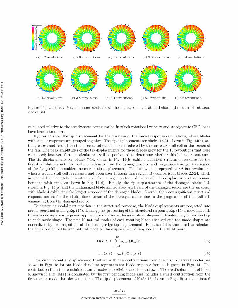
Unsteady Mach number contours at the mid-chord are shown in Figs. 13(a)-13(j) for 10 equally spacedtime-steps spanning the first 5.6 revolutions of the unsteady calculation. The corresponding total pressureratio and referred mass flow rate at these time-steps are indicated by the fine vertical lines in Fig. 12(a).Limited flow unsteadiness is evident in the vicinity of the damaged blades. In contrast, significant unsteadi-ness is apparent in much of the undamaged sector, with the greatest level of flow unsteadiness occurring inthe blade passages between blade 16 and blade 21.

The stalled flow emanating from the damaged sector, denoted a stall cell and identified by the blueregions, is the dominant unsteady flow effect in Figs. 13. In Fig. 13(b), the stall cell covers roughly a thirdof the fan wheel, from blade 21 to blade 5, and the mass flow rate is near its maximum. From Fig. 13(c)to 13(g), the stall cell regresses slightly before propagating opposite the direction of rotation until half of theblade tips are stalled, from blade 15 to blade 5. At this point, the mass flow rate is at a minimum due tothe partially blocked blade passages associated with the stalled flow. Subsequently from Fig. 13(h) to 13(j),the stall cell detaches from the damaged sector, progresses opposite the direction of rotation, and dissipatesas the flow recovers and the mass flow rate increases to the maximum value. In addition, as the stall cellpropagates at the blade tips, the Mach number in the inner span of the corresponding blade passage alsodecreases, indicating a loss of mass flow through a majority of the blade passages.

B. Forced Response of the Damaged Fan

The forced response calculations of the bird damaged fan are presented in this section. The time-dependentaerodynamic loads are extracted from the unsteady CFD calculations and transferred to the structural solverat each time-step using the one-way forced response framework. The forced response calculations wereperformed for 5,000 time-steps corresponding to 10 revolutions of the fan. The circumferential displacement,uθR, at the leading edge of the blade tips is used as an indicator of the blade response. The displacement is

15 of 24


Dow

nloa

ded

by U

nive

rsity

of

Mic

higa

n -

Dud

erst

adt C

ente

r on

Dec

embe

r 13

, 201

7 | h

ttp://

arc.

aiaa

.org

| D

OI:

10.

2514

/6.2

014-

0334

(a) 0.2 revolutions. (b) 0.8 revolutions. (c) 1.4 revolutions. (d) 2.0 revolutions. (e) 2.6 revolutions.

(f) 3.2 revolutions. (g) 3.8 revolutions. (h) 4.4 revolutions. (i) 5.0 revolutions. (j) 5.6 revolutions.

Figure 13: Unsteady Mach number contours of the damaged blade at mid-chord (direction of rotation:clockwise).

calculated relative to the steady-state configuration in which rotational velocity and steady-state CFD loadshave been introduced.

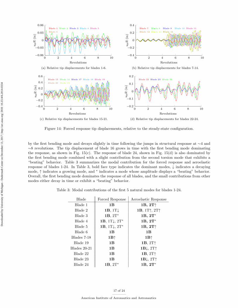
Figures 14 show the tip displacement for the duration of the forced response calculations, where bladeswith similar responses are grouped together. The tip displacements for blades 15-21, shown in Fig. 14(c), arethe greatest and result from the large aerodynamic loads produced by the unsteady stall cell in this region ofthe fan. The peak amplitudes of the tip displacements for these blades grow for the 10 revolutions that werecalculated; however, further calculations will be performed to determine whether this behavior continues.The tip displacements for blades 7-14, shown in Fig. 14(b) exhibit a limited structural response for thefirst 4 revolutions until the stall cell releases from the damaged sector and progresses through this regionof the fan yielding a sudden increase in tip displacement. This behavior is repeated at ∼8 fan revolutionswhen a second stall cell is released and progresses through this region. By comparison, blades 22-24, whichare located immediately downstream of the damaged sector, exhibit smaller tip displacements that remainbounded with time, as shown in Fig. 14(d). Finally, the tip displacements of the damaged blades 1-5,shown in Fig. 14(a) and the undamaged blade immediately upstream of the damaged sector are the smallest,with blade 4 exhibiting the largest response of the damaged blades. Overall, the most significant structuralresponse occurs for the blades downstream of the damaged sector due to the progression of the stall cellemanating from the damaged sector.

To determine modal participation in the structural response, the blade displacements are projected intomodal coordinates using Eq. (15). During post-processing of the structural response, Eq. (15) is solved at eachtime-step using a least squares approach to determine the generalized degrees of freedom, qm correspondingto each mode shape. The first 10 natural modes of each rotating blade are used and the mode shapes arenormalized by the magnitude of the leading edge tip displacement. Equation 16 is then used to calculatethe contribution of the mth natural mode to the displacement of any node in the FEM mesh.

U(x, t) ≈10∑

m=1

qm(t)Φm(x) (15)

Um(x, t) = qm(t)Φm(x, t) (16)

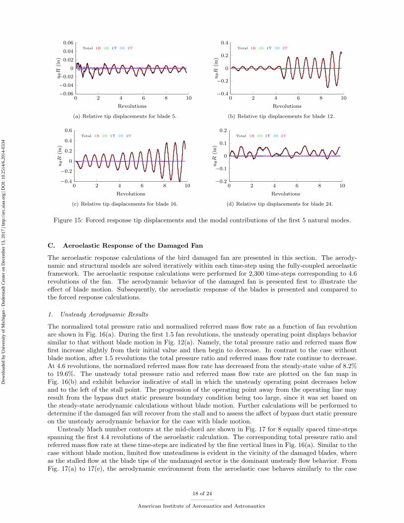
The circumferential displacement together with the contributions from the first 5 natural modes areshown in Figs. 15 for one blade that best represents the blade response from each group in Figs. 14. Thecontribution from the remaining natural modes is negligible and is not shown. The tip displacement of blade5, shown in Fig. 15(a) is dominated by the first bending mode and includes a small contribution from thefirst torsion mode that decays in time. The tip displacement of blade 12, shown in Fig. 15(b) is dominated

16 of 24


Dow

nloa

ded

by U

nive

rsity

of

Mic

higa

n -

Dud

erst

adt C

ente

r on

Dec

embe

r 13

, 201

7 | h

ttp://

arc.

aiaa

.org

| D

OI:

10.

2514

/6.2

014-

0334

0 2 4 6 8 10−0.06

−0.03

0

0.03

0.06

Revolutions

uθR

(in

)

Blade 1 Blade 2 Blade 3 Blade 4 Blade 5

Blade 6

(a) Relative tip displacements for blades 1-6.

0 2 4 6 8 10−0.4

−0.2

0

0.2

0.4

Revolutions

uθR

(in

)


Blade 12 Blade 13 Blade 14

(b) Relative tip displacements for blades 7-14.

0 2 4 6 8 10−0.4

−0.2

0

0.2

0.4

0.6

Revolutions

uθR

(in

)


Blade 20 Blade 21

(c) Relative tip displacements for blades 15-21.

0 2 4 6 8 10−0.2

−0.1

0

0.1

0.2

Revolutions

uθR

(in

)


(d) Relative tip displacements for blades 22-24.

Figure 14: Forced response tip displacements, relative to the steady-state configuration.

by the first bending mode and decays slightly in time following the jumps in structural response at ∼4 and∼8 revolutions. The tip displacement of blade 16 grows in time with the first bending mode dominatingthe response, as shown in Fig. 15(c). The response of blade 24, shown in Fig. 15(d) is also dominated bythe first bending mode combined with a slight contribution from the second torsion mode that exhibits a“beating” behavior. Table 3 summarizes the modal contribution for the forced response and aeroelasticresponse of blades 1-24. In Table 3, bold face type indicates the dominant modes, ↓ indicates a decayingmode, ↑ indicates a growing mode, and ∗ indicates a mode whose amplitude displays a “beating” behavior.Overall, the first bending mode dominates the response of all blades, and the small contributions from othermodes either decay in time or exhibit a “beating” behavior.

Table 3: Modal contributions of the first 5 natural modes for blades 1-24.

Blade Forced Response Aeroelastic Response

Blade 1 1B 1B, 2T↑Blade 2 1B, 1T↓ 1B, 1T↑, 2T↑Blade 3 1B, 2T∗ 1B, 2T∗

Blade 4 1B, 1T↓, 2T∗ 1B, 2T∗

Blade 5 1B, 1T↓, 2T∗ 1B, 2T↑Blade 6 1B 1B

Blades 7-18 1B↑ 1B↑Blade 19 1B 1B, 2T↑

Blades 20-21 1B 1B↓, 2T↑Blade 22 1B 1B, 2T↑Blade 23 1B 1B↓, 2T↑Blade 24 1B, 2T∗ 1B, 2T∗

17 of 24


Dow

nloa

ded

by U

nive

rsity

of

Mic

higa

n -

Dud

erst

adt C

ente

r on

Dec

embe

r 13

, 201

7 | h

ttp://

arc.

aiaa

.org

| D

OI:

10.

2514

/6.2

014-

0334

0 2 4 6 8 10−0.06

−0.04

−0.02

0

0.02

0.04

0.06

Revolutions

uθR

(in

)

Total 1B 2B 1T 3B 2T

(a) Relative tip displacements for blade 5.

0 2 4 6 8 10−0.4

−0.2

0

0.2

0.4

Revolutions

uθR

(in

)


(b) Relative tip displacements for blade 12.

0 2 4 6 8 10−0.4

−0.2

0

0.2

0.4

0.6

Revolutions

uθR

(in

)


(c) Relative tip displacements for blade 16.

0 2 4 6 8 10−0.2

−0.1

0

0.1

0.2

Revolutions

uθR

(in

)


(d) Relative tip displacements for blade 24.

Figure 15: Forced response tip displacements and the modal contributions of the first 5 natural modes.

C. Aeroelastic Response of the Damaged Fan

The aeroelastic response calculations of the bird damaged fan are presented in this section. The aerody-namic and structural models are solved iteratively within each time-step using the fully-coupled aeroelasticframework. The aeroelastic response calculations were performed for 2,300 time-steps corresponding to 4.6revolutions of the fan. The aerodynamic behavior of the damaged fan is presented first to illustrate theeffect of blade motion. Subsequently, the aeroelastic response of the blades is presented and compared tothe forced response calculations.

1. Unsteady Aerodynamic Results

The normalized total pressure ratio and normalized referred mass flow rate as a function of fan revolutionare shown in Fig. 16(a). During the first 1.5 fan revolutions, the unsteady operating point displays behaviorsimilar to that without blade motion in Fig. 12(a). Namely, the total pressure ratio and referred mass flowfirst increase slightly from their initial value and then begin to decrease. In contrast to the case withoutblade motion, after 1.5 revolutions the total pressure ratio and referred mass flow rate continue to decrease.At 4.6 revolutions, the normalized referred mass flow rate has decreased from the steady-state value of 8.2%to 19.6%. The unsteady total pressure ratio and referred mass flow rate are plotted on the fan map inFig. 16(b) and exhibit behavior indicative of stall in which the unsteady operating point decreases belowand to the left of the stall point. The progression of the operating point away from the operating line mayresult from the bypass duct static pressure boundary condition being too large, since it was set based onthe steady-state aerodynamic calculations without blade motion. Further calculations will be performed todetermine if the damaged fan will recover from the stall and to assess the affect of bypass duct static pressureon the unsteady aerodynamic behavior for the case with blade motion.

Unsteady Mach number contours at the mid-chord are shown in Fig. 17 for 8 equally spaced time-stepsspanning the first 4.4 revolutions of the aeroelastic calculation. The corresponding total pressure ratio andreferred mass flow rate at these time-steps are indicated by the fine vertical lines in Fig. 16(a). Similar to thecase without blade motion, limited flow unsteadiness is evident in the vicinity of the damaged blades, whereas the stalled flow at the blade tips of the undamaged sector is the dominant unsteady flow behavior. FromFig. 17(a) to 17(e), the aerodynamic environment from the aeroelastic case behaves similarly to the case

18 of 24


Dow

nloa

ded

by U

nive

rsity

of

Mic

higa

n -

Dud

erst

adt C

ente

r on

Dec

embe

r 13

, 201

7 | h

ttp://

arc.

aiaa

.org

| D

OI:

10.

2514

/6.2

014-

0334

0 1 2 3 4 50.8

0.84

0.88

0.92

0.96

Revolutions

Norm

alize

dV

alu

e

mR PR

(a) Referred mass flow rate and total pressure ratiotime history.

0.8 0.84 0.88 0.92 0.96 10.88

0.92

0.96

1


Norm

alize

dP

ress

ure

Rati

o

Operating Line

Undamaged

Damaged Char. Curve

Steady Damaged

Unsteady Damaged

(b) Fan map with characteristic curve and steady andunsteady operating points.

Figure 16: Unsteady total pressure ratio and referred mass flow rate from aeroelastic calculations.

without blade motion. Specifically, in Fig. 17(b) the stall cell emanating from the damaged sector coversroughly a third of the fan wheel, from blade 20 to blade 5, and the mass flow rate is near its maximum.From Fig. 17(c) to 17(e), the stall cell detaches from the damaged sector, progresses opposite the directionof rotation, and dissipates at in Fig. 17(f). At this point, the flow fails to recover and a stalled region formsin Fig. 17(h) that encompasses 5/6 of the blade tips accompanied with a further decrease in referred massflow rate. Overall, the influence of the structural response of the aerodynamic behavior of the damaged fanis evident, with the blade motion causing stalled flow for a majority of the fan.

(a) 0.2 revolutions. (b) 0.8 revolutions. (c) 1.4 revolutions. (d) 2.0 revolutions.

(e) 2.6 revolutions. (f) 3.2 revolutions. (g) 3.8 revolutions. (h) 4.4 revolutions.

Figure 17: Unsteady Mach number contours of the damaged blade at mid-chord from aeroelastic calcula-tions(direction of rotation: clockwise).

2. Aeroelastic Blade Response

The circumferential displacement, uθR, at the leading edge of the blade tips is presented in Figs. 18 for theduration of the aeroelastic response calculations. The displacement is calculated relative to the steady-stateconfiguration in which rotational velocity and steady-state CFD loads have been introduced, and blades

19 of 24


Dow

nloa

ded

by U

nive

rsity

of

Mic

higa

n -

Dud

erst

adt C

ente

r on

Dec

embe

r 13

, 201

7 | h

ttp://

arc.

aiaa

.org

| D

OI:

10.

2514

/6.2

014-

0334

with similar responses are grouped together. Overall, the aeroelastic response of the fan blades is similarto the forced response results, particularly for the undamaged blades. The largest tip displacements occurfor blades 15-21 and grow in time, as shown in Fig. 18(a). In Fig. 18(b), blades 7-14 exhibit a limitedstructural response for the first 2 revolutions until the stall cell releases from the damaged sector andprogresses through this region of the fan yielding a sudden increase in tip displacement. Between 3.8 and4.4 fan revolutions, a large region of stalled flow progresses through to region resulting in a second increasein tip displacement. In Fig. 18(d), blades 22-24 exhibit smaller tip displacements that remain bounded withtime. When compared to the forced response results in Fig. 14(d), the tip displacements for blades 22-24are smaller in magnitude and contain a higher frequency content that indicates a higher structural mode isparticipating in the response of these blades. Finally, the tip displacements of blades 1-6 in Fig. 18(a) arethe smallest; however, the aeroelastic response of these blades contains a higher frequency component thanthose from the forced response calculation shown in Fig. 14(a).

0 1 2 3 4 5−0.06

−0.03

0

0.03

0.06

Revolutions

uθR

(in

)


Blade 6

(a) Relative tip displacements for blades 1-6.

0 1 2 3 4 5−0.4

−0.2

0

0.2

0.4

Revolutions

uθR

(in

)



(b) Relative tip displacements for blades 7-14.

0 1 2 3 4 5−0.4

−0.2

0

0.2

0.4

0.6

Revolutions

uθR

(in

)


Blade 20 Blade 21

(c) Relative tip displacements for blades 15-21.

0 1 2 3 4 5−0.2

−0.1

0

0.1

0.2

Revolutions

uθR

(in

)


(d) Relative tip displacements for blades 22-24.

Figure 18: Aeroelastic response tip displacements, relative to the steady-state configuration.

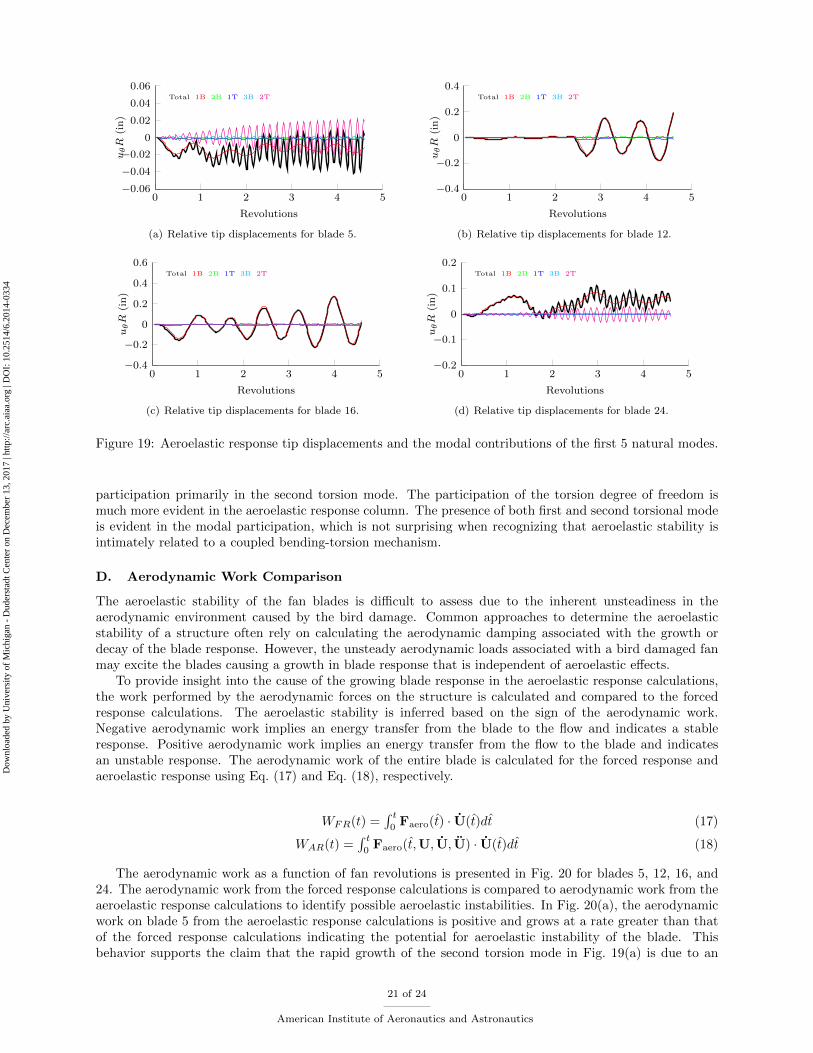
The circumferential displacement together with the contributions from the first 5 natural modes areshown in Figs. 19 for the same representative blades in Fig. 15. Similar to the forced response results, the tipdisplacement of blade 12, shown in Fig. 19(b) is dominated by the first bending mode and decays slightly intime following the jump in structural response at ∼2 revolutions. Furthermore, the tip displacement of blade16 in Fig. 19(c) grows in time with the first bending mode dominating the response. The tip displacement ofblade 5, shown in Fig. 19(a), is initially dominated by the first bending mode. However, the second torsionmode grows rapidly in time and dominates the blade response after ∼2 fan revolutions. The rapid growthof the second torsion mode is unique to the aeroelastic response of blade 5 and may indicate an aeroelasticinstability. The response of blade 24 in Fig. 19(d) is also initially dominated by the first bending mode;however, after ∼1 revolution, the second torsion mode becomes increasingly dominant and the amplitudeexhibits a “beating” behavior that is more significant than that of the forced response results.

Overall, the first bending mode is dominant in the forced response and aeroelastic response of all blades,with the amplitude of this mode growing for blades 7-18 due to the unsteady stall cell downstream of thedamaged sector. The tip displacements from the aeroelastic response calculations also contain contributionsfrom the first and second torsion mode that may be significant (as in the case of blades 1, 3-5, and 24) andmay grow in time or exhibit “beating”. Comparison of the two columns in Table 3 reveals some fundamentaldifferences between the forced response and aeroelastic response of the damaged fan. For the forced responsecase, the primary response of the blade is in the fundamental bending mode, with occasional minor torsional

20 of 24


Dow

nloa

ded

by U

nive

rsity

of

Mic

higa

n -

Dud

erst

adt C

ente

r on

Dec

embe

r 13

, 201

7 | h

ttp://

arc.

aiaa

.org

| D

OI:

10.

2514

/6.2

014-

0334

0 1 2 3 4 5−0.06

−0.04

−0.02

0

0.02

0.04

0.06

Revolutions

uθR

(in

)


(a) Relative tip displacements for blade 5.

0 1 2 3 4 5−0.4

−0.2

0

0.2

0.4

Revolutions

uθR

(in

)


(b) Relative tip displacements for blade 12.

0 1 2 3 4 5−0.4

−0.2

0

0.2

0.4

0.6

Revolutions

uθR

(in

)


(c) Relative tip displacements for blade 16.

0 1 2 3 4 5−0.2

−0.1

0

0.1

0.2

Revolutions

uθR

(in

)


(d) Relative tip displacements for blade 24.

Figure 19: Aeroelastic response tip displacements and the modal contributions of the first 5 natural modes.

participation primarily in the second torsion mode. The participation of the torsion degree of freedom ismuch more evident in the aeroelastic response column. The presence of both first and second torsional modeis evident in the modal participation, which is not surprising when recognizing that aeroelastic stability isintimately related to a coupled bending-torsion mechanism.

D. Aerodynamic Work Comparison

The aeroelastic stability of the fan blades is difficult to assess due to the inherent unsteadiness in theaerodynamic environment caused by the bird damage. Common approaches to determine the aeroelasticstability of a structure often rely on calculating the aerodynamic damping associated with the growth ordecay of the blade response. However, the unsteady aerodynamic loads associated with a bird damaged fanmay excite the blades causing a growth in blade response that is independent of aeroelastic effects.

To provide insight into the cause of the growing blade response in the aeroelastic response calculations,the work performed by the aerodynamic forces on the structure is calculated and compared to the forcedresponse calculations. The aeroelastic stability is inferred based on the sign of the aerodynamic work.Negative aerodynamic work implies an energy transfer from the blade to the flow and indicates a stableresponse. Positive aerodynamic work implies an energy transfer from the flow to the blade and indicatesan unstable response. The aerodynamic work of the entire blade is calculated for the forced response andaeroelastic response using Eq. (17) and Eq. (18), respectively.

WFR(t) =∫ t

0Faero(t) · U(t)dt (17)

WAR(t) =∫ t

0Faero(t,U, U, U) · U(t)dt (18)

The aerodynamic work as a function of fan revolutions is presented in Fig. 20 for blades 5, 12, 16, and24. The aerodynamic work from the forced response calculations is compared to aerodynamic work from theaeroelastic response calculations to identify possible aeroelastic instabilities. In Fig. 20(a), the aerodynamicwork on blade 5 from the aeroelastic response calculations is positive and grows at a rate greater than thatof the forced response calculations indicating the potential for aeroelastic instability of the blade. Thisbehavior supports the claim that the rapid growth of the second torsion mode in Fig. 19(a) is due to an

21 of 24


Dow

nloa

ded

by U

nive

rsity

of

Mic

higa

n -

Dud

erst

adt C

ente

r on

Dec

embe

r 13

, 201

7 | h

ttp://

arc.

aiaa

.org

| D

OI:

10.

2514

/6.2

014-

0334

aeroelastic mechanism. The aerodynamic work from the forced response for blade 5 is also positive and growsslowly in time, demonstrating that the unsteady aerodynamic loading contributes energy to the blade. Theaerodynamic work from the forced response and aeroelastic response calculations for blades 12 and 16 aresimilar, as shown in Figs. 20(b) and 20(c). For these blades, the aerodynamic work from both cases growsslowly with time at approximately the same rate, suggesting that the growth in blade response is due to theunsteady aerodynamic loads caused by the stall cell rather than an aeroelastic instability. The aerodynamicwork for blade 24 from the aeroelastic response calculations is predominantly negative compared to theforced response case, as shown in Fig. 20(d). This suggests that the aeroelastic effects produce positiveaerodynamic damping. Overall, the aerodynamic work from the aeroelastic response calculations is similarto that from the forced response calculations except for blade 5. The growth in blade response for all bladesappears to be dominated by the unsteady aerodynamics caused by the damaged blades, with the exceptionbeing blade 5 that exhibits a possible aeroelastic instability of the second torsion mode.

0 2 4 6 8 10−5

0

5

10

15

Revolutions

Work

(lb

f-in

)

Forced Response Aeroelastic

(a) Aerodynamic work for blade 5.

0 2 4 6 8 10

0

100

200

Revolutions

Work

(lb

f-in

)


(b) Aerodynamic work for blade 12.

0 2 4 6 8 10

0

100

200

300

Revolutions

Work

(lb

f-in

)


(c) Aerodynamic work for blade 16.

0 2 4 6 8 10

−20

0

20

40

Revolutions

Work

(lb

f-in

)


(d) Aerodynamic work for blade 24.

Figure 20: Comparison of aerodynamic work from the forced response and aeroelastic response calculations.

VII. Concluding Remarks

The forced response and aeroelastic response of a bird-damaged fan is examined using a coupled compu-tational fluid dynamics (CFD) and computational structural dynamics (CSD) framework. The aerodynamicmodel is based on the ANSYS CFX code, which is used to perform the steady-state and unsteady CFD calcu-lations for a bird-damaged fan. Subsequently, ANSYS Mechanical APDL is coupled with ANSYS CFX usingthe ANSYS Multifield solver to perform a one-way forced response and fully-coupled aeroelastic responsecalculations of a bird-damaged fan. The damaged configuration resembles a realistic bird strike damage thatcovers a sector of 5 fan blades in which the damage includes substantial leading-edge deformation and globalbending and untwist of the blades.

The steady-state CFD calculations of the damaged fan show a flow loss of 8.2% and the characteristiccurve indicates that the damaged fan is operating near stall where unsteadiness in the flow is significant.Furthermore, the aerodynamic behavior of the damaged fan exhibits unsteadiness, particularly in the regiondownstream of the damaged sector where a stall cell emanating from the damaged sector progresses at theblade tips.

The forced response calculations show that the undamaged blades downstream of the damaged sector

22 of 24


Dow

nloa

ded

by U

nive

rsity

of

Mic

higa

n -

Dud

erst

adt C

ente

r on

Dec

embe

r 13

, 201

7 | h

ttp://

arc.

aiaa

.org

| D

OI:

10.

2514

/6.2

014-

0334

exhibit the greatest blade tip displacement and the amplitude of the displacement grows in time. The bladetip displacements for all blades are dominated by the first bending mode, and the tip displacement for thedamaged blades also include small contributions from the first and second torsion modes.

The structural response resulting from the fully-coupled aeroelastic calculations is similar to that fromthe forced response calculations. The largest tip displacement occurs for the undamaged blades downstreamof the damaged sector and the amplitudes grow in time. The structural response of all blades is dominated bythe first bending mode; however, contributions from the second torsion mode are significant for the damagedblades. Specifically, the amplitude of the second torsion mode grows rapidly in time for the upstreamdamaged blade.

The aerodynamic work exerted by the aerodynamic forces is calculated and compared for both the forcedresponse and aeroelastic calculations. In general, the growth in blade response appears to be due to theunsteady aerodynamic loads caused by the damaged fan blades rather than by an aeroelastic mechanism.However, the aerodynamic work for the upstream damaged blade suggests that the rapid growth of secondtorsion mode may be due to an aeroelastic instability.

References

1Teichmann, H. C. and Tadros, R. N., “Analytical and Experimental Simulation of Fan Blade Behavior and DamageUnder Bird Impact,” Journal of Engineering for Gas Turbines and Power , Vol. 113, No. 4, October 1991, pp. 582–594.

2Isomura, K. and Giles, M. B., “A Numerical Study of Flutter in Transonic Fan,” Journal of Turbomachinery, Vol. 120,No. 3, July 1998, pp. 500–507.

3Horsley, J., “The ‘Rolls-Royce’ Way of Validating Fan Integrity,” AIAA Paper No. 93-2602, AIAA/SAE/ASME/ASEE29th Joint Propulsion Conference and Exhibit , Monterey, CA, June 1993, pp. 1–22.

4Bendiksen, O. O., “Aeroelastic Problems in Turbomachines,” Transactions of the ASME , Vol. 113, October 1991, pp. 582–594.

5Bendkisen, O. O., Kielb, R. E., and Hall, K. C., “Turbomachinery Aeroelasticity,” Encyclopedia of Aerospace Engineering,John Wiley & Sons, 2010.

6Eschenfelder, P., “Jet Engine Certification Standards,” Proceedings of the International Bird Strike Committee, Amster-dam, April 2000, pp. 535–540.

7Howard, W. D., “Turbofan Engine Bird Ingestion Testing,” AIAA Paper No. 1991-2380, Proceedings of the 27th JointPropulsion Conference, Sacramento, CA, June 1991.

8Kim, M., Vahdati, M., and Imregun, M., “Aeroelastic Stability Analysis of a Bird-Damaged Aeroengine Assembly,”Journal of Aerospace Sciences and Technologies, Vol. 5, No. 7, 2001, pp. 469–482.

9Imregun, M. and Vahdati, M., “Aeroelastic Analysis of a Bird-Damaged Fan Assembly Using a Large Numerical Model,”The Aeronautical Journal , Vol. 103, No. 1030, December 1999, pp. 569–578.

10Goyal, V. K., Huertas, C. A., Borrero, J. R., and Leutwiler, T. R., “Robust Bird-Strike Modeling Based on ALE For-mulation Using LS-DYNA,” AIAA Paper No. 2006-1759, Proceedings of the 47th AIAA/ASME/ASCE/AHS/ASC Structures,Structural Dynamics, and Materials Conference, Newport, RI, May 2006.

11Hirschbein, M. S., “Bird Impact Analysis Package for Tubine Engine Fan Blades,” AIAA Paper No. 1982-696, Proceedingsof the 23rd AIAA/ASME/ASCE/AHS/ASC Structures, Structural Dynamics, and Materials Conference, New Orleans, LA,May 1982.

12Mao, R., Meguid, S. A., and Ng, T. Y., “Finite Element Modeling of a Bird Striking an Engine Fan Blade,” Journal ofAircraft , Vol. 44, No. 2, 2007, pp. 583–596.

13Mao, R., Meguid, S. A., and Ng, T. Y., “Transient Three Dimensional Finite Element Analysis of a Bird Striking a FanBlade,” International Journal of Mechanics and Materials in Design, Vol. 4, No. 1, 2008, pp. 79–96.

14Meguid, S. A., Mao, R., and Ng, T. Y., “FE Analysis of Geometry Effects of an Artificial Bird Striking an AeroengineFan Blade,” International Journal of Impact Engineering, Vol. 35, No. 6, 2008, pp. 487–498.

15Nizampatnam, L. S. and Horn, W. J., “Investigation of Equation of State Models for Predicting Bird Impact Loads,”AIAA Paper No. 2008-682, Proceedings of the 46th AIAA Aerospace Sciences Meeting and Exhibit , Reno, NV, January 2008.

16Shimamura, K., Shibue, T., and Grosch, D. J., “Numerical Simulation of Bird Strike Damage on Jet Engine Fan Blade,”Proceedings of the ASME/JSME Pressure Vessels and Piping Conference, San Diego, CA, July 2004.

17Aotsuka, M. and Tsuchiya, N., “Numerical Simulation of Transonic Fan Flutter with 3-D N-S CFD Code,” Proceedingsof the ASME Turbo Expo 2008: Power for Land, Sea, and Air , Berlin, Germany, June 2008.

18Marshall, J. G. and Imregun, M., “A Review of Aeroelasticity Methods with Emphasis on Turbomachinery Applications,”Journal of Fluids and Structures, Vol. 10, No. 3, 1996, pp. 237–267.

19Muir, E. R. and Friedmann, P. P., “Unsteady Aerodynamic Analysis of a Bird-Damaged Turbofan,” AIAA Paper No.2013-1773, Proceedings of the 54th AIAA/ASME/ASCE/AHS/ASC Structures, Structural Dynamics, and Materials Confer-ence, Boston, MA, April 2013.

20Muir, E. R. and Friedmann, P. P., “Unsteady Aerodynamic Loading on Bird-Damaged Fan Blades and Its Effect onForced Response,” Proceedings of the 2013 International Forum on Aeroelasticity and Structural Dynamics, Bristol, UK, June2013.

21Morris, A., Allen, C., and Rendall, T., “CFD-based Optimization of Aerofoils Using Radial Basis Functions for Domain

23 of 24


Dow

nloa

ded

by U

nive

rsity

of

Mic

higa

n -

Dud

erst

adt C

ente

r on

Dec

embe

r 13

, 201

7 | h

ttp://

arc.

aiaa

.org

| D

OI:

10.

2514

/6.2

014-

0334

Element Parameterization and Mesh Deformation,” International Journal for Numerical Methods in Fluids, Vol. 58, No. 8,2008, pp. 827–860.

22van Zuijlen, A., de Boer, A., and Bijl, H., “Higher-order Time Integration Through Smooth Mesh Deformation for 3DFluid-Structure Interaction Simulations,” Journal of Computational Physics, Vol. 224, No. 1, 2007, pp. 414–430.

23Jakobsson, S. and Amoignon, O., “Mesh Deformation Using Radial Basis Functions for Gradient Based AerodynamicShape Optimization,” Computers and Fluids, Vol. 36, No. 6, 2007, pp. 1119–1136.

24Buhmann, M. D., Radial Basis Functions: Theory and Implementations, Cambridge University Press, Cambridge, 2003.25de Boer, A., van der Schoot, M., and Bijl, H., “Mesh deformation based on radial basis function interpolation,” Computers

& Structures, Vol. 85, No. 11, 2007, pp. 784–795.26Lamorte, N. and Friedmann, P. P., “Hypersonic Aeroelastic Stability Boundary Computations using Radial Basis Func-

tions for Mesh Deformation,” AIAA Paper No. 2012-5943, Proceedings of the 18th AIAA/3AF International Space Planes andHypersonic Systems and Technologies Conference, Tours, France, September 2012.

27Mechanical APDL Theory Reference Guide - Version 14.5 , ANSYS, Inc., 2012.28Hilber, H. M., Hughes, T. J. R., and Taylor, R. L., “Improved Numerical Dissipation for Time Integration Algorithm in

Structural Dynamics,” Earthquake Engineering and Structural Dynamics, Vol. 5, No. 3, July-September 1977, pp. 283–292.29Mechanical APDL Coupled-Field Analysis Guide - Version 14.5 , ANSYS, Inc., 2012.

24 of 24


Dow

nloa

ded

by U

nive

rsity

of

Mic

higa

n -

Dud

erst

adt C

ente

r on

Dec

embe

r 13

, 201

7 | h

ttp://

arc.

aiaa

.org

| D

OI:

10.

2514

/6.2

014-

0334

aeroelastic response of bird-damaged fan blades using a

Documents