aerosol optical thickness retrieval over land and water...

Aerosol optical thickness retrieval over land and water using

Global Ozone Monitoring Experiment (GOME) data

J. Kusmierczyk-Michulec1 and G. de LeeuwPhysics and Electronics Laboratory, Netherlands Organization for Applied Scientific Research, The Hague, Netherlands

Received 16 March 2004; revised 29 July 2004; accepted 3 August 2004; published 3 March 2005.

[1] An algorithm for the retrieval of the aerosol optical thickness over land and overwater from Global Ozone Monitoring Experiment (GOME) data is presented. Thecloud fraction in the GOME pixels is determined using the Fast Retrieval Scheme forClouds From the Oxygen A Band (FRESCO) algorithm. Surface contributions to thetop of atmosphere reflectance are determined from the GOME surface reflectancedatabase. The aerosol retrieval algorithm uses lookup tables that were created usingthe radiative transfer model 6S. The algorithm allows retrieving the aerosol typescharacterized by Angstrom coefficients in the range from �0.1 to 2.8; i.e., the rangeof values observed by the AERONET ground-based measurements. Validation of thealgorithm done using the AERONET Sun photometer data for 12 sites in Europeand Africa, for the year 1997, shows very good agreement. The correlationcoefficient between the satellite retrieval and AERONET data for the wavelength of440 nm is 97%, and for 670 nm it is 94%. Validation of the algorithm for the year2000 was done for a few sites with similar results. The algorithm has beensuccessfully tested over an island influenced by Saharan dust (i.e., Cape Verde, 16�N,22�W) and over a site located near the Saharan desert (i.e., Bondoukoui, 11�N, 3�W).For other sites located near the Saharan desert such as Bidi Bahn (14�N, 2�W)and Banizombou (13�N, 2�E), the agreement was very good at 440 nm. Thealgorithm has not been tested over other bright surfaces such as ice-coveredregions. Examples of the spatial distribution of the aerosol optical thickness overEurope, north Africa, and the North Atlantic for the year 1997 and 2000 arepresented.

Citation: Kusmierczyk-Michulec, J., and G. de Leeuw (2005), Aerosol optical thickness retrieval over land and water using Global

Ozone Monitoring Experiment (GOME) data, J. Geophys. Res., 110, D10S05, doi:10.1029/2004JD004780.

1. Introduction

[2] The atmosphere and its composition, especiallydust and smoke, have been intensively investigated sincethe beginning of the 20th century [Gibbs, 1929]. Therelation between the amount of dust particles andmeteorological phenomena has been studied by Aitken[1890]; air pollution in towns has been described, e.g.,by Fyfe [1911] and Cohen and Ruston [1912].Nowadays, in the epoque of satellite observations, aero-sols are still a subject of interest because of theirproperties as well as their influence on climate [e.g.,Brasseur et al., 1999].[3] Aerosols regulate the solar radiative transfer in the

atmosphere, causing a change in the net radiation at the topof the atmosphere, as well as changes in horizontal visibil-ity. Recent model calculations indicate that aerosol particles

emitted during fossil fuel (e.g., soot) and biomass (organicaerosols) burning, as well as ammonium sulphate and nitrateaerosols, can contribute to the anthropogenic radiativeforcing of climate [e.g., Charlson et al., 1991]. However,because the residence time of emitted aerosols is relativelyshort, in comparison to that of greenhouse gases [e.g.,Schwartz, 1996], the climatic influences of aerosols aremost important in the immediate vicinity of the sourceregions.[4] Satellites are best suited to determine the spatial

distribution of aerosols over large areas during extendedtime periods, needed to evaluate their effects. Satelliteobservations since more than 25 years provide the aerosolindex (AI) from the Total Ozone Mapping Spectrometer(TOMS) [Herman et al., 1997] and, over the oceans, theaerosol optical thickness (AOT) from the Advanced VeryHigh Resolution Radiometer (AVHRR). Instruments be-come more and more sophisticated, reaching the compro-mise between spatial and spectral resolution, i.e., theModerate Resolution Imaging Spectrometer (MODIS)[Kaufman and Tanre, 1996].[5] Usually, instruments used for aerosol retrieval are

designed for this purpose, such as Along Track Scanning

JOURNAL OF GEOPHYSICAL RESEARCH, VOL. 110, D10S05, doi:10.1029/2004JD004780, 2005

1On leave from Institute of Oceanology, Polish Academy of Sciences,Sopot, Poland.

Copyright 2005 by the American Geophysical Union.0148-0227/05/2004JD004780$09.00

D10S05 1 of 15

Radiometer 2 (ATSR-2) or Medium Resolution ImagingSpectrometer (MERIS). In this paper we explore the use ofinstruments with high spectral resolution, designed foraccurate gas phase retrieval, such as GOME, ScanningImaging Absorption Spectrometer for Atmospheric Charto-graphy (SCIAMACHY) and Ozone Monitoring Instrument(OMI). Because calibrated SCIAMACHY data are not yetavailable, OMI is planned to be launched in the summer of2004 therefore GOME data are used in this study. A seriousdisadvantage is the large GOME pixel size resulting in avery low probability of clear sky pixels which limits theusefulness of GOME for aerosol retrieval, as will be shown.Hence this study must be regarded as a preparation for theretrieval of aerosol properties from SCIAMACHY.[6] GOME is a 4-channel grating spectrometer, operating

in the wavelength range of 237–794 nm with a spectralresolution of 0.2–0.4 nm [Burrows et al., 1999]. On 21April 1995, GOME was launched onboard the ERS-2satellite into a near-polar Sun-synchronous orbit at a meanaltitude of about 785 km, with a mean local equator crossingtime of 1030 (local time). GOME performs nadir observa-tions by scanning the surface from east (�30�) to west (30�)in 4.5 s. One across-track scan is divided into three 1.5 sscans, resulting in three GOME ground pixels with anaverage coverage of 40 km � 320 km. For about 10% ofthe time, the swath is reduced to 240 km, and all pixel sizesare four times smaller. Once per day the Sun is observedover a diffuser plate for radiometric calibration.[7] The application of GOME data to obtain the aerosol

maps over water has been presented by Guzzi et al. [2001].Holzer-Popp et al. [2002] have suggested the combinedapproach using two instruments: GOME and ATSR-2. Here,an algorithm to derive the aerosol optical thickness fromGOME data over both water and land is presented. Theadvantage of this approach is that it uses only GOME dataand the surface reflectance database [Koelemeijer et al.,2003] that is also a GOME product. The algorithm uses thelookup tables (LUTs) that were created using the radiativetransfer model 6S [Vermote et al., 1997] for three mainaerosol types: maritime, continental and urban [McClatcheyet al., 1984]. However, the algorithm allows to retrieveaerosol mixtures characterized by Angstrom coefficients inthe range from �0.1 to 2.8, i.e., the values observed by theAERONET ground-based measurements [Dubovik et al.,2002].[8] Detailed information about the Aerosol Robotic

Network (AERONET) is presented in the work of Holbenet al. [1998]. The description of the data processing andcloud-screening algorithm used by the AERONET ispresented in the work of Eck et al. [1999] and Smirnovet al. [2000].

2. Theory

[9] The total radiance L received by a sensor at the top ofthe atmosphere can be presented as the sum of the contri-butions from aerosols, molecules, and the surface. Instead ofradiance L, it is often more convenient to use reflectance,i.e., a dimensionless function, defining the ratio of themeasured radiance L to the solar flux at the top of theatmosphere: r = pL/ms Fs, where ms = cosqs, qs is the solarzenith angle and Fs is the extraterrestrial solar irradiance. In

both representations the molecular contribution is assumedto be well known. The main issue is the separation of theaerosol and surface contributions to the total reflectance.[10] The reflectance at the top of atmosphere above a

Lambertian homogeneous surface with reflectance rsurfviewed by a satellite sensor and illuminated by Sun canbe described as follows [Tanre et al., 1979]

rTOA qs; qv;Djð Þ ¼ Tg qs; qvð Þ ratm þ T# qsð ÞT" qvð Þrsurf

1� Srsurf

( )

ð1Þ

The independent parameters in equation (1) are defined asfollows:

qs, js zenith and azimuth angles of the directsunlight;

qv, jv view zenith and azimuth angles from aspacecraft toward Earth’s surface;

Dj = js � jv;rTOA the total apparent reflectance measured at the

satellite level;ratm the atmospheric reflectance;

S the spherical albedo of the atmosphere, i.e.,the normalized irradiance backscatteredby the atmosphere when the input irradianceat the bottom is isotropic;

rsurf the surface reflectance (land or water);Tg the gaseous transmission;

T#(qs), T"(qv) the total transmission of the atmosphere

on the path between the Sun and thesurface, and respectively, the surface andthe sensor.

2.1. Atmospheric Transmission Functions

[11] The total transmission of the atmosphere on the pathbetween the Sun and the surface T#(qs), respectively be-tween the surface and the sensor T"(qv), can be presented asthe product of the Rayleigh transmission function Tr [e.g.,Lenoble, 1985] and the aerosol transmission function Ta.2.1.1. Rayleigh Transmission Functions[12] The analytical formulae for the Rayleigh transmis-

sion function can be obtained by applying the Eddingtonapproximation to the radiative transfer equation [Lenoble,1985]:

Tr m;lð Þ ¼ 2=3þ mð Þ þ 2=3� mð Þ exp �tr lð Þ=mð Þ4=3þ tr lð Þ ; ð2Þ

where m = cos q (q is the solar/view zenith angle), tr is theRayleigh optical thickness. Equation (2) is used in theradiative transfer model 6S.2.1.2. Aerosol Transmission Functions[13] The aerosol transmission functions were calculated

using the radiative transfer model 6S [Vermote et al., 1997]for the following input parameters: (1) solar/view zenithangles q: 0�, 10�, 20�, 30�, 35�, 40�, 45�, 50�, 55� and 60�;(2) wavelengths l: 380 nm, 440 nm, 463 nm, 495 nm,555 nm and 670 nm; (3) aerosol types: maritime, continen-tal and urban [McClatchey et al., 1984]; and (4) aerosoloptical thickness ta(555 nm): 0, 0.1, 0.2, 0.3, 0.4, 0.55, 0.8

D10S05 KUSMIERCZYK-MICHULEC AND DE LEEUW: AEROSOL RETRIEVAL

2 of 15

D10S05

and 1.Next, an empirical formula, which form was indicatedby equation (2), was fitted to these discrete values to allowfor a fast and a very accurate calculation of all intermediatevalues. The maximum relative error between the empiricalformula (see equation (3)) and the 6S results is ±0.0003(±0.03%).

Ta l; m; hð Þ ¼ exp � ta l; hð Þ4m

� � X3i¼1

ti m;lð Þtia l; hð Þ þ 1

( ); ð3Þ

where h = ta(555). The functions ti(m) for a given l dependon m and the aerosol type.

2.2. Spherical Albedo of the Atmosphere

[14] The spherical albedo of the atmosphere was calcu-lated using the radiative transfer model, for the same inputparameters as in the case of the aerosol transmittance(section 2.2). The values were approximated by third-orderpolynomials

S l; hð Þ ¼X3m¼0

sm lð Þtma l; hð Þ: ð4Þ

For ta ! 0 the spherical albedo of the atmosphere reachesthe value of the spherical albedo for the molecularscattering: S(l, h) ! SR(l), i.e., s0(l) ! SR(l).

2.3. Atmospheric Reflectance

[15] The atmospheric reflectance ratm is the sum of themolecular reflectance, called Rayleigh’s reflectance rr,aerosol reflectance ra, and the coupling term rra, whichtakes into account the interaction between molecules andaerosols. The relation between the atmospheric reflectanceratm, and the aerosol optical thickness ta, for differentwavelengths l, and the scattering angle Q that is a functionof the zenith angles qs, qv, and the azimuth angle Dj = js �jv, may be written in a general form as:

ratm l;Qð Þ ¼ 1

4 cos qs cos qu

X4i¼0

Bi l;Qð Þtia l; hð Þ: ð5Þ

The values of Bi depend on the aerosol type, the wavelengthand the scattering angle. The number of terms in equation (5)depends on the aerosol type and the wavelength.

3. Description of the Algorithm

[16] The GOME aerosol retrieval algorithm uses themeasured TOA reflectances, averaged over a 1nm widewavelength window, and centered at 380 nm, 440 nm,463 nm, 495 nm, 555 nm and 670 nm.[17] The calibration procedure of the raw GOME TOA

radiances is described in detail by Koelemeijer et al. [2003].The altitude correction of land pixels was done using theinformation about the ground pressure, that was found fromthe ETOPO-5 database [Haxby et al., 1983]. The solar andviewing angles were averaged over the GOME groundpixels. Pixels with solar zenith angles larger than 60� werediscarded.

Table 1. Overview of the Values of Real n(l) and Imaginary Parts

k(l) of the Refractive Index, As Well As Single Scattering Albedo

w(l) for the Basic Aerosol Components Used in the WCP Model

[McClatchey et al., 1984]

l, nm w(l) n(l) k(l)

Dust-Like Particles380 0.62 1.53 0.008440 0.63 1.53 0.008463 0.64 1.53 0.008495 0.64 1.53 0.008555 0.65 1.53 0.008670 0.67 1.53 0.008

Water-Soluble Particles380 0.96 1.53 0.005440 0.96 1.53 0.005463 0.96 1.53 0.005495 0.96 1.53 0.005555 0.96 1.53 0.006670 0.95 1.53 0.006

Oceanic Particles380 1.0 1.39 4.5E-8440 1.0 1.38 8.3E-9463 1.0 1.38 7.5E-9495 1.0 1.38 5.7E-9555 1.0 1.38 4.3E-9670 1.0 1.38 3.7E-8

Soot Particles380 0.28 1.75 0.463440 0.25 1.75 0.456463 0.24 1.75 0.453495 0.23 1.75 0.450555 0.21 1.75 0.440670 0.17 1.75 0.430

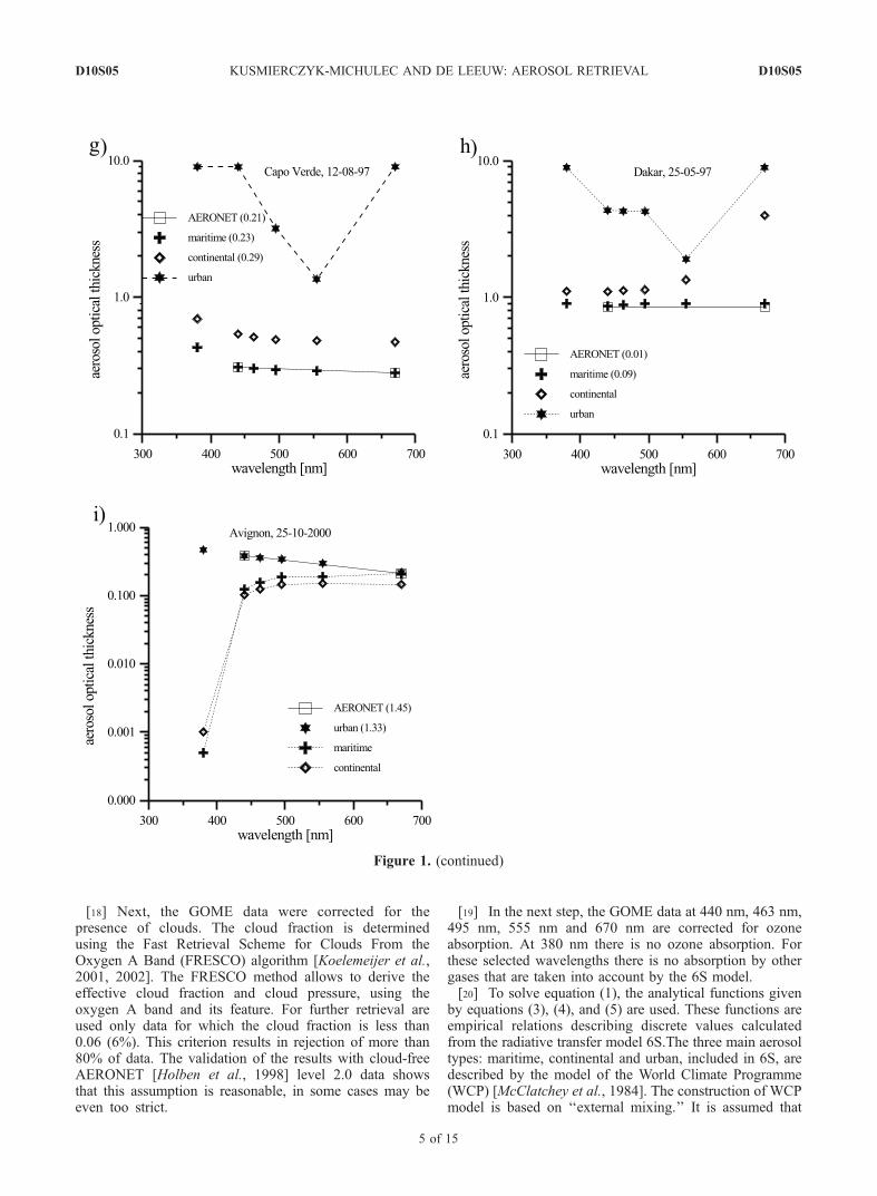
Figure 1. Each time the aerosol optical thickness is calculated from the atmospheric reflectance, assuming three possibleaerosol types: maritime, continental and urban. The solution is marked as an ‘‘output.’’ The known aerosol optical thicknessthat corresponds to the known atmospheric reflectance (input) is also plotted. The calculations are performed for thescattering angle Q = 140�. The input aerosol type is: (a) urban, (b) continental, (c) maritime, (d) biomass, and (e) desertdust. (f) The error, defined as a difference between the desert dust aerosol type and the maritime aerosol type. Also shown isan illustration of the retrieval process using the real measurements: (g) The Angstrom coefficient for the maritime aerosoltype is 0.23, i.e., very close to the measured one (0.21). The continental aerosol type also gives very similar value of theAngstrom coefficient (0.29), but this value is outside the continental domain (see section 3.1). The urban aerosol type givesunrealistic spectrum; therefore it is rejected. Therefore our algorithm selects the maritime aerosol type. (h) Similar situationas in Figure 1g. In addition, the continental aerosol type gives a very unrealistic spectrum; therefore it is rejected. (i) Bothmaritime and continental aerosol types have very strange spectral behavior. The Angstrom coefficient for the urban aerosoltype gives a reasonable value; therefore this aerosol type is selected.


3 of 15

D10S05

Figure 1


4 of 15

D10S05

[18] Next, the GOME data were corrected for thepresence of clouds. The cloud fraction is determinedusing the Fast Retrieval Scheme for Clouds From theOxygen A Band (FRESCO) algorithm [Koelemeijer et al.,2001, 2002]. The FRESCO method allows to derive theeffective cloud fraction and cloud pressure, using theoxygen A band and its feature. For further retrieval areused only data for which the cloud fraction is less than0.06 (6%). This criterion results in rejection of more than80% of data. The validation of the results with cloud-freeAERONET [Holben et al., 1998] level 2.0 data showsthat this assumption is reasonable, in some cases may beeven too strict.

[19] In the next step, the GOME data at 440 nm, 463 nm,495 nm, 555 nm and 670 nm are corrected for ozoneabsorption. At 380 nm there is no ozone absorption. Forthese selected wavelengths there is no absorption by othergases that are taken into account by the 6S model.[20] To solve equation (1), the analytical functions given

by equations (3), (4), and (5) are used. These functions areempirical relations describing discrete values calculatedfrom the radiative transfer model 6S.The three main aerosoltypes: maritime, continental and urban, included in 6S, aredescribed by the model of the World Climate Programme(WCP) [McClatchey et al., 1984]. The construction of WCPmodel is based on ‘‘external mixing.’’ It is assumed that

Figure 1. (continued)


5 of 15

D10S05

both continental and urban aerosol types are composed ofsoot, water-soluble and dust-like particles, mixed with theproper volume percentage of each component. The per-centage contribution of soot particles is taken as 1% inthe continental aerosol type and 22%, in the urbanaerosol type. The maritime aerosol type is composed ofsea-salt particles (95%) and water-soluble particles (5%).The values of real n(l) and imaginary parts k(l) of therefractive index, as well as single scattering albedo w(l)for the basic aerosol components used in the WCP modelare listed in Table 1.[21] The main idea of the aerosol retrieval algorithm is that

after correction for the surface contribution to the TOAreflectance (described in section 3.2), the solution of equa-tion (1) is searched in three domains of possible solutions:maritime, continental and urban, applying a bisection pro-cedure [Press et al., 1992]. The threshold values of theaerosol optical thickness at 380 nm and 440 nm are assumedto be 1.5, for the other wavelengths, is 1.

3.1. Selection of the Most Probable Aerosol Type

[22] In order to select the most plausible aerosol type thespectral dependence of the aerosol optical thickness, and theexpected range of values of the Angstrom coefficients a fora given aerosol type are taken into account. We assume thatfor predominantly ‘‘maritime’’ aerosol, the Angstrom coef-ficient a 2h�0.1; 0.65i, for predominantly ‘‘continental’’aerosol a 2h0.65; 1.32i, and for predominantly ‘‘urban’’aerosol a 2h1.32; 2.8i. This distinction is based on earlierstudies on the relations between the aerosol composition,and the values of the Angstrom coefficients [Kusmierczyk-Michulec et al., 1999, 2001, 2002; Kusmierczyk-Michulecand Marks, 2000].[23] Figures 1a–1e show five model simulations. Each

time the aerosol optical thickness is calculated from theatmospheric reflectance, assuming three possible aerosoltypes: maritime, continental and urban. The solution ismarked as an ‘‘output.’’ The known aerosol optical thick-ness accompanying the known atmospheric reflectance(input) is also plotted for comparison. The calculationspresented here were performed for the scattering angleQ = 140�. It is noted that such model simulations werealso done for other possible scattering angles, and theresults were similar.[24] If the ‘‘true’’ type is the urban aerosol type

(Figure 1a) the ‘‘maritime’’ and ‘‘continental’’ solutionsdo not resemble the typical power law curves. This effectis independent of the value of the aerosol optical thickness.If the ‘‘true’’ aerosol type is continental (Figure 1b),maritime (Figure 1c) or a mixed continental maritime, thenboth curves, i.e., one representing the maritime solution andthe second describing the continental solution, are parallel(on the logarithmic scale), characterized by nearly the samevalues of the Angstrom coefficient. However, the ‘‘urban’’solution reaches extremely high values, especially in the UVregion.[25] Figures 1d and 1e present situations when the ‘‘true’’

aerosol type is outside the LUT. In both cases the aerosoloptical thickness and the atmospheric reflectance represent-ing biomass (Figure 1d) and desert dust (Figure 1e) aerosoltypes were created using 6S, and the biomass burningaerosol model is deduced from measurements taken by

Sun photometers in Amazonia; however, the desert dustaerosol model is described in the work of Shettle [1984].[26] In both situations the true aerosol types have to be

described by their substitutes: the biomass aerosol type bythe continental solution, and the desert dust aerosol type bythe maritime solution. The question arises what error isinvolved. In case of the biomass aerosol type, the value ofthe Angstrom coefficient (in the range 440 nm to 670 nm) is1.3649. The value of the Angstrom coefficient given by themaritime solution is 1.156, and by the continental solution1.307. The first value is outside the domain of the maritimesolutions, therefore is rejected. The second value belongs tothe domain of the ‘‘continental’’ solutions, therefore isselected. The absolute error is 0.01 for 440 nm, 0.002 for670 nm, and for 380 nm is a bit higher, 0.02. Figure 1fshows the error being the result of replacement the ‘‘true’’desert dust aerosol type by the maritime solutions. It is clearthat the smaller value of the aerosol optical thickness, AOD(555), the smaller is the error. The smallest error is in therange of wavelengths between 440 nm (around 0.006) and495 nm (around 0.02), the biggest error is for 380 nm and670 nm (around 0.04). It means that this approach can beapplicable in the small range of wavelengths, especially at440 nm, because the error is negligible.[27] The retrieval process using the real observation data

is illustrated in Figures 1g and 1i. However, the maritimeand continental aerosol types may have very similar matchwith the TOA reflectance, the distinction between them ispossible and is based on comparison of their Angstromcoefficients.

Figure 2. Example of the contribution of the surface term,i.e., T"T#*Rsurf/(1 � S Rsurf) to the TOA reflectance for12 months evaluated for a pixel in Poland (50�N, 20�E).Calculations are performed for the scattering angle Q =120�; the continental aerosol type and the aerosol opticalthickness AOD(555) = 0.4. The very high contribution forJanuary, February, and March is due to the presence ofsnow.


6 of 15

D10S05

3.2. Surface Correction

[28] One of the crucial issues is the proper surfacecorrection, especially over land. Thus the selection ofwavelengths in the spectral range between 380 nm and670 nm was not coincidental. The reason was that in thatrange the contribution of the surface term, i.e., T"T#*Rsurf/(1 � S Rsurf) (see equation (1)) to the TOA reflectance is nothigher than 60% (except in the case of snow). Thiscontribution increases with wavelength reaching a value

of around 80% at 770 nm (see Figure 2). These numbers arebased on the analysis of the surface reflectances taken fromthe GOME surface reflectance database [Koelemeijer et al.,2003].[29] In this database are stored the minimum Lambert

equivalent reflectivity (LER) values which occurred in theperiod June 1995 and December 2000. LER [Dave, 1977;Bhartia et al., 1993] is the value of the Lambertian spectralsurface albedo for which the modeled and measured reflec-

Table 2. Summary of Intercomparison Between the GOME Retrieval and the AERONET Sun Photometer Dataa

Site Location Period N1 jDt(440)j R1 N2 jDt(670)j R2

Banizombou 13N, 2E January toOctober 1997

5 0.028 0.99 — — —

Bondoukoui 11N, 3W January toDecember 1997

27 0.043 0.95 14 0.034 0.96

Barbados 13N, 59W January toNovember 1997

7 0.031 0.89 6 0.037 0.99

Capo Verde 16N, 22W January toDecember 1997

8 0.024 0.98 7 0.018 0.99

Rame Head 50N, 4W April to July1997

6 0.054 0.86 5 0.055 0.97

Bidi Bahn 14N, 2W January to September1997

12 0.066 0.90 — — —

Dakar 14N, 16W January to July1997

6 0.061 0.94 1 0.018 —

GSFC 39N, 76W February toNovember 1997

13 0.045 0.89 — — —

Lille 50N, 3E June toSeptember 1997

4 0.032 0.97 3 0.034 —

Ispra 45N, 8E August toNovember 1997

4 0.059 0.92 3 0.044 —

Bermuda 32 N, 64W December 1997 2 0.008 — 1 0.002 —Aire Adour 43N, 0E February to

November 19978 0.037 0.72 8 0.053 0.50

aHere N1 and N2 are the number of samples at wavelengths of 440 nm and 670 nm. jDt(440)j and jDt(670)j are the mean absolute differences betweensatellite and Sun photometer measurements at 440 and 670 nm, respectively. R1 and R2 are the correlation coefficients between the GOME and AERONETaerosol optical thickness values at 440 and 670 nm, respectively. The correlation coefficients are given for N � 4.

Figure 3. Comparison of the GOME retrieved aerosol optical thickness and the AERONET Sunphotometer measurements at (a) 440 nm and (b) 670 nm. Also shown is an intercomparison for threemain aerosol types: (c and d) maritime, (e and f) continental, and (g and h) urban.


7 of 15

D10S05

Figure 3. (continued)


8 of 15

D10S05

Figure 4. Time series of the aerosol optical thickness retrieved from GOME (diamonds) and measuredby Sun photometers (crosses) in 1997: (a) Bondoukoui, 440 nm; (b) Bondoukoui, 670 nm; and (c) BidiBahn, 440 nm.


9 of 15

D10S05

tance at the top of the atmosphere are equal, assuming aRayleigh scattering atmosphere above a Lambertian surfacein the radiative transfer model. Bhartia et al. [1993] andHerman and Celarier [1997] show that LER may beregarded as an estimate of the value of the bidirectionalreflectance distribution function (BRDF). Therefore we usethis value as equivalent to rsurf in equation (1).[30] The GOME database includes information of the

surface reflectance for a given wavelength and month ofthe year, with a spatial resolution of 1 � 1�. In the case ofthe large GOME pixels, using this database is more efficient

than trying to differentiate between different types ofvegetation and soils. If the value from the database doesnot allow to solve equation (1) then a bisection method iscombined with an iteration method [Press et al., 1992]. Thevalues of the surface reflectance are checked in the rangebetween 0 and Rsurf, where the upper limit is indicated bythe value from the GOME database. If the value of Rsurf

from the GOME database causes that the surface term ishigher than the input TOA reflectance, then iteratively Rsurf

is lowered in each next step by 10% until equation (1) canbe solved. The lowest value of Rsurf is 0. There is no

Figure 5. Comparison of the aerosol optical thickness retrieved from GOME with the Sun photometermeasurements in Capo Verde in 1997. (a) An example of the ‘‘spectral’’ variation, (b) time series for440 nm, and (c) time series for 670 nm.


10 of 15

D10S05

correction for the opposite situation: the surface reflectancefrom the database is much lower than the real one. Suchsituation took place in case of very bright surface. In thatcase too little surface reflectance was subtracted and theaerosol optical thickness was much higher than the thresh-old value.[31] Over water, the proper surface correction is also

important, especially in the UV and the visible part ofspectrum. In that range the contribution of the water-leavingreflectance to the TOA reflectance is the most significant,around 60%, depending on the type of water and atmo-sphere. This contribution decreases with the wavelength,reaching at 670 nm around 1–8%. For Case I waters[Morel, 1988], i.e., mainly oceanic waters which opticalproperties are determined by phytoplankton and their im-mediate derivatives, the contribution at 670 nm will bealmost negligible, because the water-leaving reflectance isclose to zero. For Case II waters [Morel, 1988], i.e., allcoastal waters which optical properties are also determinedby the presence of sediments or dissolved yellow substances,this contribution can be much higher.[32] In addition to the correction for the water-leaving

reflectance also the Sun glint correction is done, using theCox and Munk [1954a, 1954b, 1955] formulae, assuming amean wind speed of 8 m/s. When the Sun glint reflectancewas higher than 0.001 the pixel was marked as Sun glintcontaminated [e.g., Veefkind and de Leeuw, 1998].

4. Validation

4.1. Comparison With Collocated Sun PhotometerMeasurements

[33] To test the accuracy of the GOME aerosolalgorithm, the retrieved aerosol optical thickness valueswere compared with collocated Sun photometer measure-ments (level 2.0), available from the AERONET Webpage (//aeronet.gsfc.nasa.gov). Validation was done for1997. Validation for 2000 was done for only a few siteswith similar results.[34] Comparison of the GOME derived aerosol optical

thickness was made for several sites (Table 2), representingdifferent types of surface, and aerosols. To avoid the cloudcontamination in the GOME aerosol retrieval, all data forwhich cloud fraction was higher than 6% were removed.Comparisons were made for the same site, day, and hour,therefore it was more difficult to find collocated measure-ments. The list of sites together with the mean absolutedifference between satellite and Sun photometer measure-ment, as well as the correlation coefficients for each site ispresented in Table 2.[35] Figures 3a and 3b show comparisons of the available

data for 1997, for the wavelengths of 440 nm and 670 nm,for all sites listed in Table 2. In some cases, for the sitescharacterized by a high surface reflectance at 670 nm (seesection 3.2 for detail), the aerosol optical thickness was notretrieved, and it is indicated in Table 2. The error bars of theGOME data were obtained from averaging over an area of0.5� � 0.5�. The high correlation gives confidence that theaerosol retrieval algorithm works well.[36] Figures 3c–3h present intercomparison for each

main aerosol type. It turns out that among all observations,

the ‘‘maritime’’ aerosol type was the most frequentlyobserved. Nevertheless, the high correlation coefficientsindicate that the retrievals have no bias for specific typesof aerosols.[37] Figures 4a–4c present comparisons of the aerosol

optical thickness retrieved from GOME and from groundmeasurements, for Bondoukoui and Bidi Bahn, for the year1997. The results show good agreement both for smallvalues of the aerosol optical thickness (around 0.05) and forhigher values (more than 0.6).[38] Figure 5a presents an example of the ‘‘spectral’’

comparison, for two AERONET wavelengths: 440 nm and670 nm, for site Capo Verde that is regarded as a represen-tation of the oceanic and dust particles. Figures 5b and 5cshow the time series of the aerosol optical thickness derivedfor 440 nm and 670 nm, respectively. This comparisonproves that the aerosol algorithm works well also for thelow values of the aerosol optical thickness.[39] Figures 6a and 6b present the ‘‘spectral’’ comparison

for two sites in Europe, in 2000: Venice (Italy) and Avignon(France). The Sun photometer in Venice has two morechannels, in the range from 380 nm to 670 nm, than thestandard ones (i.e., 380 nm and 500 nm), therefore thecomparison was also possible for the UV values (Figure 6a).

4.2. Sources of Uncertainty in the Aerosol OpticalThickness

[40] One of the main sources of uncertainty in theretrieval of aerosol optical thickness is the surface reflec-tance. On the other hand, errors in the radiometric calibra-tion of GOME and errors caused by residual cloudcontamination lead to uncertainty in the derived LERvalues. Koelemeijer et al. [2003] estimated for the LibyanDesert site that the absolute errors in the derived LERvalues due to degradation in optical components of theGOME instrument do not exceed 0.01–0.02 for all wave-lengths except 335 nm. This implies that for other, lessbright, areas absolute errors should be smaller.[41] The next source of discrepancy between the derived

aerosol optical thickness and Sun photometer measurements(see Table 2) is related to the pixel size. The ground Sunphotometer measurements are assumed to be representativefor the whole GOME pixel area of 40 � 320 km2. Thisimplies that variations between the retrieved and the mea-sured values of the aerosol optical thickness might becaused by variability in the area observed by GOME (orpresence of small clouds). Owing to the large GOME pixelsize the classical approach to the surface correction basedon the vegetation index NDVI would not be sufficientbecause GOME pixels are often inhomogeneous due topresence of surfaces with different reflectances throughoutthe pixel. Therefore the application of the GOME surfacereflectance database is more accurate.[42] To estimate the absolute error in the surface reflec-

tance from the GOME database the ‘‘effective’’ surfacereflectance was calculated for each AERONET site(Tables 2 and 3). Using the aerosol optical thicknessmeasured by the Sun photometers and the TOA reflectancefrom GOME, the ‘‘effective’’ surface reflectance for thepixel area observed by GOME was calculated (equation (1)).The results are presented in Table 3. The absolute errorvaries with wavelength and geographical location. The


11 of 15

D10S05

results indicate that in many cases the values in the GOMEdatabase were underestimated. As was mentioned in section3.2 we do not correct for this situation. The largest discrep-ancy was found for the Banizombou site, i.e., 0.075 at670 nm. The high underestimation in the surface reflectanceat this wavelength resulted in a large overestimation of theretrieved aerosol optical thickness. Because the resultingvalue was much higher than the threshold it was rejected(see section 3). However, the mean absolute error in thesurface reflectance does not exceed 0.03 at 440 nm and0.029 at 670 nm.[43] There are other sources of uncertainties in the aerosol

optical thickness, e.g., related to specific aerosol models.However, all these errors are already taken into account bycomparing real measurements and retrieved values andlisted in Table 2 as absolute errors. The mean absolute errorfor the aerosol optical thickness at 440 nm is 0.04 and at670 nm it is 0.03.

5. Aerosol Optical Thickness Spatial Distribution

[44] Having established that the algorithm providesreliable results as determined from comparison withAERONET Sun photometer data over Europe and Africa,the spatial distribution of the aerosol optical thicknessvalues over this part of the world has been determined for1997 and 2000. The data are presented for the region of theNorth Atlantic and Europe (i.e., latitude from 5�N to 70�Nand longitude from 80�W to 70�E). Over Europe there areregions with high values of the aerosol optical thickness dueto anthropogenic activities as well as rural regions where theaerosol optical thickness is low [Robles Gonzalez et al.,2000]. Over Africa, Sahara desert dust dominates, and it istransported over the Atlantic throughout the year [e.g.,Chiapello and Moulin, 2002]. In the winter, there is also a

strong transport of carbonaceous aerosols from Africanregion north of the equator [Herman et al., 1997].[45] Owing to the large fraction of cloud contaminated

pixels, only few valid data are left. Therefore the data havebeen combined to represent three periods, i.e., the ‘‘Euro-pean summer,’’ i.e., May, June, July, and August (MJJA),the ‘‘European winter,’’ i.e., January, February, November,and December (JFND) and the other months, i.e., March,April, September, and October (MASO), to representthe interseasonal changes. The results are presented onFigures 7a–7e, for the wavelength of 440 nm.[46] Figures 7a and 7b present the ‘‘winter’’ spatial

distribution of the aerosol optical thickness for the year1997 and 2000. For latitudes higher than 40�N there is nodata because of two reasons: presence of clouds and

Figure 6. Comparison of the aerosol optical thickness retrieved from GOME with the Sun photometermeasurements in 2000: (a) Venice and (b) Avignon.

Table 3. Absolute Error in the Surface Reflectance for the Same

AERONET Sites As in Table 2a

Site Location jDrsurf (440)j jDrsurf(670)jBanizombou 13N, 2E 0.039 0.075Bondoukoui 11N, 3W 0.018 0.015Barbados 13N, 59W 0.021 0.014Capo Verde 16N, 22W 0.025 0.023Rame Head 50N, 4W 0.016 0.006Bidi Bahn 14N, 2W 0.025 0.045Dakar 14N, 16W 0.063 0.049GSFC 39N, 76W 0.035 0.031Lille 50N, 3E 0.051 0.023Ispra 45N, 8E 0.042 0.036Bermuda 32 N, 64W 0.007 0.009Aire Adour 43N, 0E 0.019 0.025

aHere jDrsurf (440)j and jDrsurf (670)j are the mean absolute differencesbetween the surface reflectance from the GOME database and the‘‘effective’’ surface reflectance calculated for a given site at 440 and670 nm, respectively. The ‘‘effective’’ surface reflectance was estimatedusing the Sun photometer measurements and the TOA reflectance fromGOME for collocated measurements.


12 of 15

D10S05

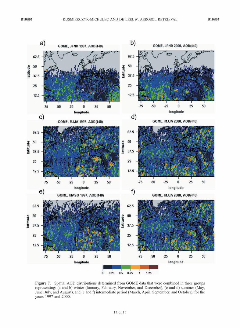
Figure 7. Spatial AOD distributions determined from GOME data that were combined in three groupsrepresenting: (a and b) winter (January, February, November, and December), (c and d) summer (May,June, July, and August), and (e and f) intermediate period (March, April, September, and October), for theyears 1997 and 2000.


13 of 15

D10S05

limitation of retrieval to data representing the solar zenithangles � 60�. The spatial distribution of the aerosol opticalthickness for both years looks very similar. The plume closeto Africa, observed also by other satellites [Myhre et al.,2004], despite of large GOME pixels, is also visible. Themean values of the aerosol optical thickness inside the plumeare in the range between 0.5 and 1. Outside the plume thevalues are much lower, around 0.25. This plume is not asclear as it is often observed from other satellite [e.g.,Bellouin, 2003]. One of the reasons could be that areaswith high AOD may be assigned as cloud contaminated. Forcomparison, Holzer-Popp et al. [2002] exclude GOMEpixels with cloud fraction above 50%, North [2002] usesATSR-2 data with cloud fraction less than 20%. When weallow for higher cloud fraction in our retrievals, the Saharandust plume is much more clearly visible. Obviously this isnot a true presentation of AOD. For instruments with smallpixels, allowing for more cloud-free pixels, this problemwill disappear.[47] Figures 7c and 7d present the ‘‘summer’’ aerosol

maps. The location of areas with high values of the aerosoloptical thickness over Africa (i.e., in the range between 0.75and 1.5), correspond also to the distribution of the highvalues of TOMS AAI (www.toms.gsfc.nasa.gov) that isrelated to the dust optical thickness [e.g., Chiapello andMoulin, 2002]. Comparison of the ‘‘summer’’ aerosol opticalthickness for Europe indicates that in 2000, in the easternpart of Europe, the values were much higher than in 1997.The spatial distribution of the aerosol optical thickness forEurope in summer 1997 is in agreement with the aerosolmap of Europe for August 1997, derived from ATSR-2[Robles Gonzalez et al., 2000]. Again the large GOMEpixels are disadvantage, because they disable the smooth,detailed spatial distribution of the aerosol optical thickness.The plume close to Africa is less visible than in winter.[48] Figures 7e and 7f present the mean values of the

aerosol optical thickness for the period of 4 months,including European spring and autumn. For that periodthe distribution of the aerosol optical thickness, for bothyears, is very similar. The location of areas with high AODover Africa resembles the situation for ‘‘summer.’’ Thevalues of the aerosol optical thickness over Europe, inspring-autumn period, for both years are much lower thanfor the summer period and their spatial distribution is moreuniform than in summer, with an exception of the eastEurope, where there are areas with high values, AOD >0.75.

6. Conclusions

[49] The GOME aerosol retrieval algorithm works well,where it can be assumed that the pixels are cloud free, suchas in the case of comparison with level 2.0 Sun photometerdata. Because of high probability of cloud contamination,therefore GOME is not suitable for monitoring aerosols on adaily or even on a monthly base. The value of GOMEaerosol data may be that they can be retrieved over land andover ocean, for the lifetime of the instrument, on a globalscale. In particular the AOD values over land are comple-mentary to the data over ocean from other instruments. TheGOME data can be retrieved from June 1995 to December2000 and the series will be extended with satellite instru-

ments covering the similar wavelengths as GOME, e.g.,SCIAMACHY, GOME-2 and OMI. The advantage of theseinstruments is the smaller pixel size allowing for less cloudcontamination and more accurate determination of thesurface reflectance. In addition, SCIAMACHY has a widerspectral range (up to 2400 nm) than GOME (up to 790 nm).The spectral information from the IR channels can beused to better discriminate dust particles and for theelimination of clouds. Moreover the unique feature ofSCIAMACHY-limb viewing geometry can be used forstratospheric retrieval.

[50] Acknowledgments. We thank the PI investigators: Didier Tanre,Brent Holben, Philippe Goloub, and Giuseppe Zibordi, and their staff forestablishing and maintaining the AERONET sites used in this investigation.We acknowledge Piet Stammes and Martin de Graaf for kindly providing usGOME data and the results from FRESCO algorithm. We thank DarekMaksimiuk for his help in solving the software problems, Roman Marks forhelpful discussion, and Marianne Degache and Robin Schoemaker for theirsupport. The algorithm was developed as part of the EO-037 project of theNational Data User Support Program of the Netherlands Space ResearchOrganization (SRON).

ReferencesAitken, J. (1890), On the number of dust particles in the atmosphere ofcertain places in Great Britain and on the continent, with remarks on therelation between the amount of dust and meteorological phenomena,Proc. R. Soc. Edinburgh, 17, 76–93.

Bellouin, M. N. (2003), Estimation de l’effect direct des aerosols a partir dela modelisation et de la teledetection passive, Ph.D. thesis, 186 pp., Univ.Sci. Technol. Lille, Lille, France.

Bhartia, P. K., J. R. Herman, and R. D. McPeters (1993), Effect of MountPinatubo aerosols on total ozone measurements from backscatter ultra-violet (BUV) experiments, J. Geophys. Res., 98, 18,547–18,554.

Brasseur, G. P., J. J. Orlando, and G. S. Tyndall (1999), AtmosphericChemistry and Global Change, 654 pp., Oxford Univ. Press, New York.

Burrows, I. P., et al. (1999), The Global Ozone Monitoring Experiment(GOME): Mission concept and first scientific results, J. Atmos. Sci.,56, 151–175.

Charlson, R. J., J. Langner, H. Rodhe, C. B. Leovy, and S. G. Warren(1991), Perturbation of the Northern Hemisphere radiative balance bybackscattering from anthropogenic sulfate aerosols, Tellus Ser. AB, 43,152–163.

Chiapello, I., and C. Moulin (2002), TOMS and METEOSAT satelliterecords of the variability of Saharan dust transport over the Atlanticduring the last two decades (1979–1997), Geophys. Res. Lett., 29(8),1176, doi:10.1029/2001GL013767.

Cohen, J. B., and A. G. Ruston (1912), Smoke: Study of Town Air, 16 pp.,Edward Arnold, London.

Cox, C., and W. Munk (1954a), Statistics of the sea surface derived fromSun glitter, J. Mar. Res., 13, 198–227.

Cox, C., and W. Munk (1954b), Measurement of the roughness of the seasurface from photographs of the Sun’s glitter, J. Opt. Soc. Am., 44, 838–850.

Cox, C., and W. Munk (1955), Some problems in optical oceanography,J. Mar. Res., 14, 63–78.

Dave, J. V. (1977), Investigation of the effect of atmospheric dust on thedetermination of total ozone from the Earth’s ultraviolet reflectivitymeasurements, NTIS-N77 – 24690 – 24692, Natl. Tech. Inf. Serv.,Springfield, Va.

Dubovik, O., B. Holben, T. F. Eck, A. Smirnov, Y. J. Kaufman, M. D. King,D. Tanre, and I. Slutsker (2002), Variability of absorption and opticalproperties of key aerosol types observed in worldwide locations, J. At-mos. Sci., 59, 590–608.

Eck, T. F., B. N. Holben, J. S. Reid, O. Dubovik, A. Smirnov, N. T. O’Neill,I. Slutsker, and S. Kinne (1999), Wavelength dependence of the opticaldepth of biomass burning, urban, and desert dust aerosol, J. Geophys.Res., 104, 31,333–31,350.

Fyfe, P. (1911), Air pollution in Glasgow and other towns in Scotland,paper presented at Conference of Smoke Abatement League of GreatBritain, Manchester, UK.

Gibbs, W. (1929), ATpo3oku (in Russian), 240 pp., Leningrad.Guzzi, R., G. Ballista, W. Di Nicolantonio, and E. Carboni (2001), Aerosolmaps from GOME data, Atmos. Environ., 35, 5079–5091.


14 of 15

D10S05

Haxby, W. F., G. D. Karner, J. L. La Brecque, and J. K. Weissel (1983),Digital images of combined oceanic and continental data sets and theiruse in tectonic studies, Eos Trans. AGU, 64, 995–1004.

Herman, J. R., and E. A. Celarier (1997), Earth surface reflectivity clima-tology at 340–380 nm from TOMS data, J. Geophys. Res., 102, 28,003–28,011.

Herman, J. R., P. K. Bhartia, O. Torres, C. Hsu, C. Seftor, and E. Celarier(1997), Global distributions of UV-absorbing aerosols from NIMBUS 7TOMS data, J. Geophys. Res., 102, 16,911–16,922.

Holben, B. N., et al. (1998), AERONET—A federated instrument networkand data archive for aerosol characterisation, Remote Sens. Environ.,66(1), 1–16.

Holzer-Popp, T., M. Schroedter, and G. Gesell (2002), Retrieving aerosoloptical depth and type in the boundary layer over land and ocean fromsimultaneous GOME spectrometer and ATSR-2 radiometer measure-ments, 1, Method description, J. Geophys. Res., 107(D21), 4578,doi:10.1029/2001JD002013.

Kaufman, Y. J., and D. Tanre (1996), Strategy for direct and indirect meth-ods for correcting the aerosol effect on remote sensing: From AVHRR toEOS-MODIS, Remote Sens. Environ., 55, 65–79.

Koelemeijer, R. B. A., P. Stammes, J. W. Hovenier, and J. F. de Haan(2001), A fast method for retrieval of cloud parameters using oxygenA band measurements from GOME, J. Geophys. Res., 106, 3475–3490.

Koelemeijer, R. B. A., P. Stammes, J. W. Hovenier, and J. F. de Haan(2002), Global distributions of effective cloud fraction and cloud toppressure derived from oxygen A band spectra measured by the GlobalOzone Monitoring Experiment: Comparison to ISCCP data, J. Geophys.Res., 107(D12), 4151, doi:10.1029/2001JD000840.

Koelemeijer, R. B. A., J. F. de Haan, and P. Stammes (2003), A database ofspectral surface reflectivity in the range 335–772 nm derived from 5.5years of GOME observations, J. Geophys. Res., 108(D2), 4070,doi:10.1029/2002JD002429.

Kusmierczyk-Michulec, J., and R. Marks (2000), The influence of sea-saltaerosols on the atmospheric extinction over the Baltic and the North Seas,J. Aerosol Sci., 31(11), 1299–1316.

Kusmierczyk-Michulec, J., O. Krueger, and R. Marks (1999), Aerosol in-fluence on the sea-viewing wide-field-of-view sensor bands: Extinctionmeasurements in a marine summer atmosphere over the Baltic Sea,J. Geophys. Res., 104(D12), 14,293–14,307.

Kusmierczyk-Michulec, J., M. Schulz, S. Ruellan, O. Krueger, E. Plate,R. Marks, G. de Leeuw, and H. Cachier (2001), Aerosol compositionand related optical properties in the marine boundary layer over theBaltic Sea, J. Aerosol Sci., 32(8), 933–955.

Kusmierczyk-Michulec, J., G. de Leeuw, and C. R. Gonzalez (2002), Em-pirical relationships between aerosol mass concentrations and Angstromparameter, Geophys. Res. Lett . , 29 (7), 1145, doi:10.1029/2001GL014128.

Lenoble, J. (1985), Radiative Transfer in Scattering and Absorbing Atmo-spheres: Standard Computational Procedures, 300 pp., A. Deepak,Hampton, Va.

McClatchey, R. A., H. J. Bolle, K. Y. Kondratyev, J. H. Joseph, M. P.McCormick, E. Raschke, J. B. Pollack, D. Spankuch, and C. Mateer(1984), A preliminary cloudless standard atmosphere for radiation com-putation, 53 pp., Int. Radiat. Comm., Boulder, Colo.

Morel, A. (1988), Optical modeling of the upper ocean in relation to itsbiogenous matter content (case I waters), J. Geophys. Res., 93, 10,749–10,768.

Myhre, G., et al. (2004), Intercomparison of satellite retrieved aerosol op-tical depth over ocean, J. Atmos. Sci., 61, 499–513.

North, P. R. J. (2002), Estimation of aerosol opacity and land surfacebidirectional reflectance from ATSR-2 dual-angle imagery: Operationalmethod and validation, J. Geophys. Res., 107(D12), 4149, doi:10.1029/2000JD000207.

Press, W. H., S. A. Teukolsky, W. T. Vetterling, and B. P. Flannery (1992),Numerical Recipes in C: The Art of Scientific Computing, 994 pp., Cam-bridge Univ. Press, New York.

Robles Gonzalez, C., J. P. Veefkind, and G. de Leeuw (2000), Aerosoloptical depth over Europe in August 1997, derived from ATSR-2 data,Geophys. Res. Lett., 27(7), 955–958.

Schwartz, S. E. (1996), The Whitehouse effect, shortwave radiative forcingof climate by anthropogenic aerosols: An overview, J. Aerosol Sci., 27,359–382.

Shettle, E. P. (1984), Optical and radiative properties of a desert aerosolmodel, in Symposium of Radiation in the Atmosphere, 74–77 pp., A.Deepak, Hampton, Va.

Smirnov, A., B. N. Holben, T. F. Eck, O. Dubovik, and I. Slutsker (2000),Cloud screening and quality control algorithms for the AERONET database, Remote Sens. Environ., 73(3), 337–349.

Tanre, D., M. Herman, P. Y. Deschamps, and A. de Leffe (1979), Atmo-spheric modeling for space measurements of ground reflectances, includ-ing bidirectional properties, Appl. Opt., 18(21), 3587–3594.

Veefkind, J. P., and G. de Leeuw (1998), A new algorithm to determine thespectral aerosol optical depth from satellite radiometer measurements,J. Aerosol Sci., 29, 1237–1248.

Vermote, E. F., D. Tanre, J. L. Deuze, M. Herman, and J.-J. Morcrette(1997), Second Simulation of the Satellite Signal in the Solar Spec-trum, 6S: An overview, IEEE Trans. Geosci. Remote Sens., 35(3),675–686.

��G. de Leeuw and J. Kusmierczyk-Michulec, Physics and Electronics

Laboratory, Netherlands Organization for Applied Scientific Research, P.O.Box 96864, N-2509 JG The Hague, Netherlands. ([email protected])


15 of 15

D10S05

aerosol optical thickness retrieval over land and water...

Documents