ARL 71-0242' NOVEMBER 1971

Aerospace Research Laboratorlos

STATISTICAL ANALYSES FOR THE WEIBULL DISTRIBUTIONWITH EMPHASIS ON CENSORED SAMPLING

LEE J. BAIN

UNIVERSITY OF MISSOURI-ROLLA

ROLLA, MISSOURI

CHARLES E. ANTLE

BARRY R. BILLMAN

PENNSYLVANIA STATE UN'IVERSITY

UNIVERSITY PAPK, PENNSY!VA11IA

CONITPACr NO. F33j1r-7.-C-1O46PROJECT NO. 707;

R~proucod by

NATIONAL TECHNICAL rIVFOR• I AT'ON SEPVICE .. ..

Sp.,rrgf.d,fo V.4 22151Approved for public release; distribution undimited.

AIR FORCE SYSTEMS COMMAND

k United States Air Forceh

\S

NOTICES

When Government drawings, specijcations, or other data are used for any purpose other than inconricetion with a definitely related Government j:rocurcinvnt operation, the United States Coverwnt'ltthereby incurs no responsibility nor any obligation whatsoever; and the fact that the Gover|'nwut ma'have formulated, furnisled, or in any way rupplied the said drawings, specifications, or other data. isnot to be regarded by implication or otherwise as in any manner licensing the holder or any otherperson or corporation, or conveying any rights or permission to manufacture, use, or sell 'my patentedinvention that may in any way be related thereto.

Agencies of the Department of Defense, qualified contractors and othergovernment agencies may obtain copies from the

Defense Documentation CenterCameron: StationAlexandria, Virginia 22314

This document has been released to the

CLEARINGHOUSEU, S. Department of CommerceSpringfield, Virginia 22151

for sale to the public.

sd~f SEVIN 0PAMfl~ Cpies, of.. '.L Technical Documentary Reports shouldI not be returned to Aerospaice- Reseairch~

•`td b o ies uni s�� rturnais reqt.ired by security considerations, contractual cbligationse or notices onaspecified dociu" nt.

AAIR /500Y7C ,o

WE

UnclassifiedSecurity Classification

DOCUMENT CONTROL DATA R & D(Security classification of title, body of abtr•cf and indexing annotation must be entered w ien the overall report is classified)

I. OntrINATING ACTIVITY (Corporate author) 24. ;.PORT SECURITY CLASSIFICATION

University of Missouri-Rolla Unclassified

Rolla, Missouri 65401 7b. GRIOUP

S. REPORT TITLE

Statistical Analyses for the Weibull Distribution with Emphasis onCensored Sampling

4. DESCRIPTIVE NOTES (Type of report and incluwive dates)

Scientific, Final.S. AU THOR(S) (Firet name, middle initial, leat name)

Lee J. Bain, Charles E. Antle and Barry R. Billman

4. REPORT DATE 7&. TOTAL NO PO AGIS 7b. NO. OF REFS

No-'ember 1971 ys?'1' 347&. 9a. ORIGINATOR'S REr*RT NUMBERMSI

b. PROJECT NO.

7071C. 9b. OTHER REPORT NO-S5 (Any other numbers thit may be assignedS~this report)

DOD Eler.zent 61102F Ahi report)d. Subelement 681304 ARL 71-02420I. OISTRIBUTION STATEMENT

Approved for public release; distribution unlimited.

It, SUPPLEMENTARY NOTES 12. SPCIN3ORING MILITARY ACTIVITY

Aerospace Research Laboratories(LB), Air Force Systems Command,

_ Wright-Patterson Air Force Base,13. AUSTIACT Ohio, 45433

This report comprises three related papers on interentikl pro-cedures tor the Weibull or extreme-value distribution based oncensored samples. In Chapter I a simple, unbiased estimator, basedon a censored sample, is proposed for the scale parameter of theextreme-value distribution. The exact distribution of the estimatoris determined for the cases in which only the fiist two or only thefirst three observations are available. The asymptotic distributlinis derived, and an approximate distribution for smail sample size isalso provided. Interval estimation for the scale parameter is devel-oped and a conservative interval estimate for reliability is alsocobtained.

Chapter II represents a continuation of the material in ChapterI with emphasis on combining independent lots. A study of thesaving in experiment time with censored sampling and a numericalexample are also presented.

In Chapter III tables are provided for obtaining confidencelimits on the parameters or reliability based on the maximum like-lihood estimators for selected censoring and sample size2s.

DD NOV ,14 73'

UnclassifiedSecurity Classirication

L4 INK A LINiK 91 LINK CKEY WO R O) ..

ROLE WT ROLE WT ROLE WY

Weibull Distribution

Extreme-'.jlue Distribution

Censored Sampling

rV

UnclassifiedýU.S.Goverurne.nt PfirIting Office! t9:1 759 080/234 SecUtity Clebtifc4t1iOn

ARL 71-0242

STATISTICAL ANALYSES FOR THE WEIBULL DISTRIBUTIONWITH EMPHASIS ON CENSORED SAMPLING

LEE 1. BAIN

UNIVERSITY OF M fSSOURI-ROLLA

ROLLA, MISSOURI 65401

CHARLES E. ANTLE

BARRY R. BILLMAN

PENNSYLVAN!A STATE UNIVERSITY

UNIVERSITY PARK, PENNSYLVANIA 16802

NOVEMBER 1971

CONTRACT F33615-71-C-1040

PROJECT 7071

AEROSPACE RESEARCH LABORATORIESAIR FORCE SYSTEMS COMMAND

UNITED STATES AIR FORCEWRIGHT-PATTERSON AIR FORCE BASE, OHIO

II

FOREWORD

'ihis final report was sponsored by the Aerospace Research

Laboratories, Air Force Systems Command, United States Air Force,

Wright-Patterson Air Force Base, Ohio, under Contract F 33615-71-

C-l040. Work on this contract wa: technically monitored by

Dr. H. Leon Harter under project 7071. Chapters I and II were

written by the principal investigator, Dr. Lee J. Bain of the

University of Missouri-Rolla, who co-authored Chapter III with

Dr. Charles E. Antle and Mr. Barry R. Billman of the Pennsylvania

State University.

iii

ABSTRACT

This report comprises three related papers on inferential

procedures for the Veibull or extreme-value distribution based on

censored samples. In Chapter I a simple, unbiased estimator,

based on a censored sample, is proposed for the scale parameter

of the extreme-value distribution. The exact distribution of the

estimator is determined for the cases in which only the first two

or only the first three observations are available. The asymptotic

distribution is derived, and an approximate distribution for small

sample size is also provided. Interval estimation for the scale

parameter is developed and a conservative interval estimate for

reliability is also obtained.

Chepter II represents a continuati,. of the material in

Chapter I with emphasis on combining independent lots. A study

of the saving in experiment time with censored sampling and a

numerical example are also presented.

In Chapter III tables are provided for obtaining confidence

limits on tl Ž parameters or reliability based on the maximum like-

lihood estimators for selected censoring and sample sizes.

iim

TABLE OF CONTENTS

Chapter Page

I Inferences Based on Censored Sampling fromthe Weibull or Extreme-value Distribution 1

II Results for One or Mcee Independent Samples 18

III Results for Censored Sampling Based onthe Maximum Likelihood Estimators 38

iv

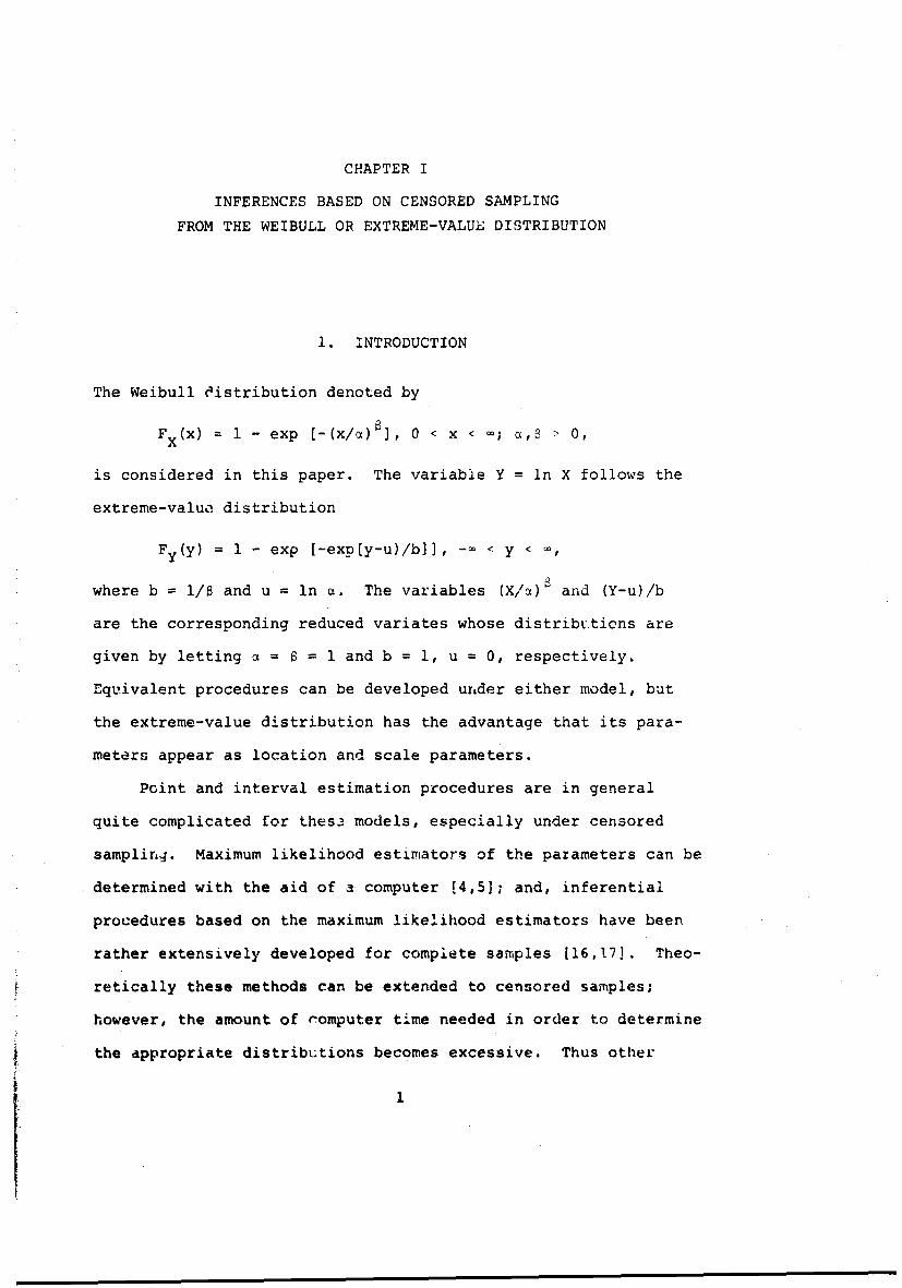
CHAPTER I

INFERENCES BASED ON CENSORED SAMPLING

FROM THE WEIBULL OR EXTREME-VALUE DISTRIBUTION

1. INTRODUCTION

The Weibull Oistribution denoted by

Fx(X) = 1 - exp [-(x/a) If 0 < x aý; o,8 0,

is considered in this paper. The variable Y = in X follows the

extreme-value distribution

Fy(y) = 1 - exp [-exp[y-u)/b]], -< y

where b = 1/8 and u = in a. The variables (X/a) 8 and (Y-u)/b

are the corresponding reduced variates whose distributions are

given by letting a = 6 = 1 and b = 1, u = 0, respectively.

Equivalent procedures can be developed under either model, but

the extreme-value distribution has the advantage that its para-

meters appear as location and scale parameters.

Point and interval estimation procedures are in general

quite complicated for these models, especially under censored

samplirn4. Maximum likelihood estimators of the parameters can be

determined with the aid of a computer E4,51; and, inferential

procedures based on the maximum likelihood estimators have been

rather extensively developed for complete samples [16,171. Theo-

retically these methods can be extended to censored samples;

however, the amount of rcomputer time needed in order to determine

the appropriate distributions becomes excessive. Thus other

i1

I • • .

estimation and hypothesis testing techniques need to be developed

for the censored sampling case.

ror point estimation one common approach has been to apply

the generalized least squares method or some related method to

obtain linear estimators of the location and scale parameters v

and b; see for example [9,10,11]. This approach for the most part

requires knowledge of the variances and covariances of the ordered

observations of the extreme-value distribution, which are avail-.

able up to n = 25 [131. It does not appear convenient to deter-

mine tests orconfidence intervals based on these point estimators

for sample sizes larger than 25. Some simple alternate point and

interval estimation procedures have been presented in [11,14] for

censored sampling. Also, Johns and Lieberman [8] have a notable

paper concerned with determining lower bounds for reliability

based on censored samples. An attempt is made in this paper to

develop procedures which are simple, reasonably good and widely

applicable without the necessity of generating an undue number of

tables.

2. INFERENCES CONCERNING b

2.1. UNBIASED ESTIMATOR OF b

Suppose xl,...,xr denote the z smallest ordered observations

in a sample of size n from the Weibull distribution. Also

yl,...yr, where yi = In xi, will represent the r smallest observa-

tions in a sample of size n from the extreme-value distribution.

The corresponding Zeduced observations will be denoted by

zi = (x./O) and wi ' (yi-u)/b.

2

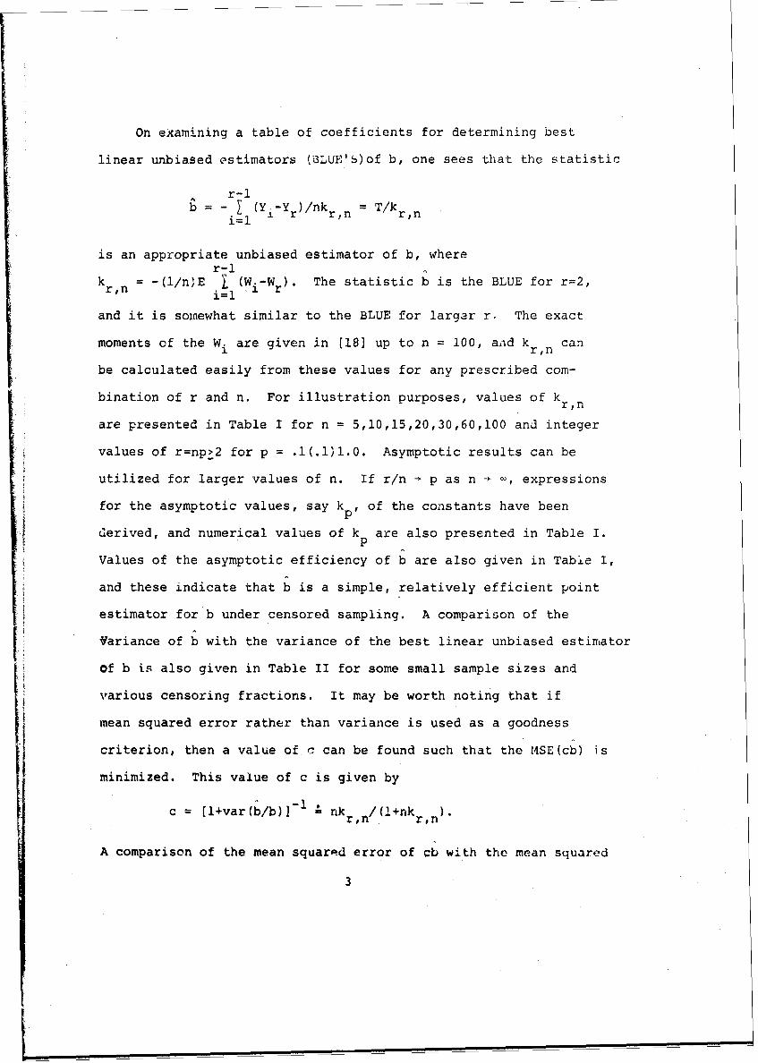
On examining a table of coefficients for determining best

linear unbiased estimators (BLUE'S)of b, one sees that the statistic

r-lb = (Yi-Yr)/nkr,n = T/kr,i=l r rn rn

is an appropriate unbiased estimator of b, wherer-l1

k = -(1/n'E ) (Wi-W r). The statistic b is the BLUE for r=2,

and it is somewhat similar to the BLUE for larger r. The exact

moments of the W. are given in [18] up to n = 100, and kr n can

be calculated easily from these values for any prescribed com-bination of r and n. For illustration purposes, values of k

r,n

are presented in Table I for n = 5,10,15,20,30,60,100 and integer

values of r=npj2 for p = .1(.1)i.0. Asymptotic results can be

utilized for larger values of n. If r/n - p as n - •, expressions

for the asymptotic values, say kp, of the constants have been

derived, and numerical values of k are also presented in Table I.p

Values of the asymptotic efficiency of b are also given in Table I,

and these indicate that b is a simple, relatively efficient point

estimator for b under censored sampling. A comparison of the

Variance of b with the variance of the best linear unbiased estimator

of b is also given in Table II for some small sample sizes and

various censoring fractions. It may be worth noting that if

mean squared error rather than variance is used as a goodness

criterion, then a value of c can be found such that the MSE(cb) is

minimized. This value of c is given by

c = [l+var(b/b)] •nk /(l+nk ).=nr,n/ (!nr,n)

A comparison of the mean squared error of cb with the mean squared

3

error of the best linear invariant estimator (BLIE) [91 of b is also

given in Table II.

2.2. SUMMARY OF DISTRIBUTION RESULTS

In considering similar tests concerning b relative to the

nuisance parameter u, one observes that attention can be re-

stricted to functions of the r - 1 statistics Yi - Yr = ln(Xi/X r);

i = l,...,r - 1. The statistic b is suggested for use since it

is a natural type of function of these statistics to consider, and

it is also a good point estimator of b under censored sampling.

Another possible indication of its desirability is that, although

it is not a sufficient statistic, it does appear as a quantity in

the joint density of the Yi - Yr" Also, since b/b is distributed

independently of all parameters, tests based on b are convenient

to express, if the appropriate percentage points are available.

The derivation of the distribution of S = exp[-nk b/bIr-i r,nH I (xi/x ) is considered in section 5.1. For r = 2, the

i=l i rdistribution of S is shown to be

F 2 (s) = ns/(s+n-l), 0 < s < 1.

Foz r = 3,

1 n! 1 1 (n- 2)(s -)

F3 (s) = (n - 3)! 2n 2(s + n - 1) 2q(s + n - 1)

_S lin (n - ýJ) (2 s + n - 2 + V/;)l ,q (n + Vq)(2s + n - 2 -)

where q= (n- 2)2 . 4s.

4

The exact distribution becomes intractable for larger r;

however, the chi-square distribution can be used to provide an

extremely good approximation. It is shown is section 5.2 that

-2 in S 2nk b/b is distributed approximately as a chi-squarer,n

variable with 2nk degrees of freedom, for r/n about .5 orrn

less.

The asymptotic distribution of T/b = -in S is also derived

in section 4. It is shown that the distribution of

/n((T/b) - p )/ap approaches a standard normal distribution as

n + and r/n ÷ p, where

Pp =

G - 2 - 2 + 2P p/A + -i+l2

- P)Ap p p p / p iSOp p

2and Ap = -in (l - p). Numerical values of kp - and p are

tabulated in Table I for p = .1(.109.

2.3 TEST OF HYPOTHESIS CONCERNING b AND POWER OF THE TEST

Consider, for example, the test of Ho: b < b0 against the

alternative HA: b > b at the a significance level. Using the

chi-square approximation stated in section 2.2, one rejects the

hypothesis H0 if

r-1 2 2 2-2 [ (Y. - Y )/b > X2(2nkn), where Prjx (v) > ' =

iir 0o C ren

Linear interpolation can be used for non-integer degrees of

freedom.

5

The power of the test for an alternative b is

(2n

Pr[reject Ho] = P[-21(Yi - Yr)/bO > X (2 n)

= PIx 2(2nk > (b /b)x (2nkr)]

r,n o r.-n

Note that a test on b is analogous to a test on the variance of a

normal distribution, since in that case (n - 1)s2 /a2 is distri-

buted as a chi-square variable with n - 1 degrees of freedom.

Thus material developed for the normal case can be applied to

this case. For example, the sample size table and o.c. curves on

2pages 299-303 of [21 are applicable by simply replacing a by b

and n by 2nk + 1.r,n

3. INFERENCES ON THE RELIABILITY

The problem of determining a test for /bor equivalently

the reliability, R = exp[-(t/a) ], will now be considered. It is

[r l X./b )X l/well known that 2rE = 2 X + (n - r + l)Xr1/b] is a

complete, sufficient statistic for a if b is known, and that

2rE/E is distributed as a chi-square variable with 2r degrees of

freedom. Since the distribution of b is independent of a, it

follows from Basu's Theorem [11 that E and b are stochastically

independent. Thus a joint confidence region can be determined

for b and R, and a conservative limit for R can be obtained. A

similar approach has been followed by Mann [9] to obtain a test

for R based on X r/X and 2rE/ý.

6

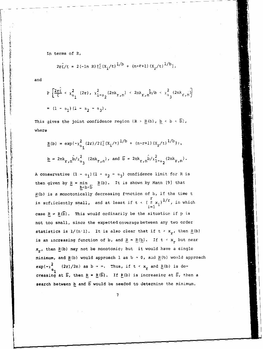
In terms of R,

2r&/= 2(-in R) [Y (Xi/t)ilb + (n-r+l) (X/t)i/b,

and

r~ý 22 A2

2(2r),x (2nk )< 2nk b/b < (2nka r,n r,n r

= (1 - ai) (i - � 2 - a3 ).

This gives the joint confidence region {R > R(b), b < b <

where

R(b) exp{-x (2r)/2[(Xi/t)i/b + (n-r+l)(X /t) 1/b,2 r

2nk b^ (2nk and b 2nk (2nkr,nb/ ,3 r,n r,n (2nk r,n)"

A conservative (1 - ai) (1 - a2 - a3) confidence limit for R is

then given by R = min R(b). It is shown by Mann [9] that- b<b<b

iR(b) is a monotonically decreasing flinction of b, if the time t•,--r 1/ris sufiiciently small, and at least if t < ( T xi in which

i=1case R - R(b). This would ordinarily be the situation if p is

not too small, since the expected coverage between any two order

statistics is i/(n'l). It is also clear that if t > xr, then R(b)

is an increasing function of b, and R = R(b). If t < x but nearr r

Xr, then R(b) may not be monotonic; but it would have a single

minimum, and R(b) would approach 1 as b ÷ 0, aad R(b) wotdld approach

exp{-x 2 (2r)/2n) as b - •'. Thus, if t < x and R(b) is de-

creasing at 9, then R = R(6). If P.(b) is increasing at E, then a

search between b and S would be needed to determine the minimum.

7

4. ASYMPTOTIC DISTRIBUTION OF b

Results given in [3] will be applied to determine the asymp-r-1

totic distribition of -T = (Yi-Y r)/n, where r/n - p as n - •. Ifi=l1r

rwe follow the notation of [3], -nT/b = in X. - r in X

n= Cin h(Xi), where the Xi are ordered exponential variables.

i=l n a1

Also, c in= 1. i = l,...,r-; Crn = -r, Cin = o, i = r + l,...,n;

F(x) I - exp(-x), h(x) = in x = H(x), H(u) - h[F- (u)] = ln[-ln(l-u)].

Also

iE(Xi = 1/(n-j+l),

j=l

ni. = [i/(n-j+l)] Ci' (E(Xi))

-1r-1

(ri-j+l)- i [ [E(Xi)I- r[E(Xr)] -H

Then

n I1n = (1/n) X c. H[E(Xji

j=lr

(1/n)j in E(Xj) - (r/n)ln E(X),

a72 = (1/n) j 2jnOn l

and the distribution of In((-T/b) - in)/n approaches a standard2 2whr

normal distribution. Furthermore, Pn -p and j 2 a 2 where

r/n - p as n- . Let

J(x) = 1, x < r/(n+l)

= 0, otherwise,

8

and let a1 = p, Ap = F (p) = -ln(l-p). Thenp

P = f J(u)H(u)du - a1h(A p0

= fo ln-ln(l-u)du i p in .

i=l p

Also,

1

((u) = (l-u)-l{U J(w)Hl (w) (l-w)dw + al-p)H' (p)},

and1

a' =fO[o(u)] 2du"

It can be shown that

a2 32 2 i i+1 2,p /(l-p)2 _2 + 2p p/p + 2 (-i)i/ii.p

Sp P p p i=l

Then the distribution of Vi((-T/b) - ip)/a approaches a standard

normal distribution.

Also, kr,n - -iDi as n - •; and the asymptotic variance of

2 2 2b is b a p/no. The asymptotic variance of the maximum likelihood

estimator of b is provided in [6] for p = .1(.1).9: and, since

this corresponds to the Cramer-Rao lower bound for an unbiased

estimator of b, the asymptotic relative efficiency of b can be

2 2calculated. Some numerical values of kp -Wp , n var b/b

and the relative efficiency of b are presented in Table I.

9

Note that, for complete samples,

nk = -Ef (in X- in X )]/ni=l n

=y+ E InX

n (ii (In i)(i''

Si=l1

where y denotes Euler's constant and numerical values of E(in Xn)

are given in [181. Also, from (15, page 71] k is approximated

by y + in in n + y/in n for large n.

5. DERIVAfION OF EXACT AND APPROXIMATE DISTRIBUTIONS

5.1. EXACT DISTRIBUTION FOR r = 2 AND r = 3

The joint density of (Xlj,...xr) is given by f(xl,...,xr)

r[n!/(n-r)!]{ H (ý/C) (xi/ 1)-i exp[-(Xi/)]) exp[-(n-r) (X r•) ],

i=l

0<X < "x " < x <1 r

On letting Ui Xi/Xr, i = 1,.. .,r - 1, the joint density of the

Ui is found to be

r-I r-lf(u 1 ,...,ur_ 1 ) = [n:Y(n-r)l] H u iui-r(r)/[ [ Ui + n - r + i]r

i=l i-i

r-I r-i Awhich involves the two quantities • U• and n Ui = exp[-nk r,nb]

i=l i=l

S Since SI/ is distributed independently of 8, 8 may be set

10

equal to one without loss of generality. For r = 2, S U1 and

the distribution of S is given directly (see also [71, [111, [121).

For r = 3, the distribution of S may be determined by making a

change of variable. The work is simplified by noting first that

the joint density of U 's and also the function S are symmetric in the1

variables. Thus, for r 3,

P[S > s]= P(U1 U2 > s. where 0 < U1 < U2 < 1,

[U1U > s], where 0 < U1 < 1, 0 < U- < 1.

Thus,

11

F 3 (s) 1 2 s s/u 2 f(ul'U2 )duldu2 "

Direct integration yields the result given earlier in the paper.

The integration becomes quite tedious for larger values of r, so

that an approximation is needed.

5.2. APPROXIMATE DISTRIBUlt-10r-i 1

The variable T = - • (Yi - Y )/n takes on positive values,i=l 1 r'

and the mean of nT/b is approximately equal to the variance of

nT/b, especially for small p. This is verified by Table I for

large n, since var(nT/b) -*na P, E(nT/b) ` kP, and k P J p in

Table I. Thus an approximate distribution with nearly the correct

first two moments is obtained by assuming that 2nT/b is distribu-

ted approximately as a chi-square variable with 2nk degrees ofr,n

freedom. The approximate percentage points were determined for

r = 2, n = 5,10,20; r = 3, n = 5,10,30, and y = .01,.05,.10,.25,

11

.50,.75,.90,.95 and .99; and the exact distributions were then

used to determine the true probabilities for these approximate

percentage points. As seen in Table III, the exact and approximate

probabilities are in very close agreement.

This chi-square approximation is also consistent with the

2asymptotic results, at least to the extent that k p -'aP Ti

follows since ((2nT/b) - 2nk )/V4n (X (v)-v)/V-2v, whichp p

becomes normally distributed as v increases; but

((2nT/b) - 2nk p)/,/4npp -- v((T/b) - k p)/a which corresponds to

the asymptotic result.

Thus the chi-square approximation seems appropriate if

substantial censoring is involved. Further work is needed to

determine the amount of error if r/n is near 1.

12

0- 0 0 H ) 0

V) N LA) r- 00 mi 0 -

r- N a N 'r N Lr CN4-) 0 H Lfl m~ H- -z co Ln r

(fl %o (.D co r- N 0 02 w2 - 0)H-- H- H- ~v N- 0 N (T) LA N- LI)

co C.. '. 0 0 0 H H H N 0) in

-Ln 00 Nl 0) 0 (1) ILn co 4*

(n Ho %D 'o a% N A N r- 0H aN (n '.0 r 0 N% N~ H) N

ECO C) '0 I,- ON N N 10 No 0 w

H D O' D m o %.D fN m ~ N '0

r- 'M '.0 '0 ýn C. NN Nen

Xn r- No N) N- o 0)

rq ý 02 N 0 No(n w. Nn v '0 N a 2 N N %D

q* ~ ~ *l l r- m H *n I n V I

0 ~ N ~ N 0 CN Nr 02 N v.

'.0~~ ~ LA m r r .N N ~ m fn m

-41 tr N Nn 0 02 '.0 Nn 02 N-- 021,

E ~ H H 00 N 0 %

'. tr -4 '.0 N A N N v a0. D N0 LA 0) a2 LA mI0 H

U) 0 C 14

0r q AC '0 C

'4.4

o w 4 r4 N o 0 s N CL -I

to 0 >4o0> 4..

13

TABLE II

Comparison of b with the BLUE and BLIE

n r V(b/b) V(BLUE/b) c nk /(l+nkr) MSE(cb/b) MSE(BI,IIL/b;

r,n r,n

3 .4175 .4168 .7055 .7064 °2945 .2942

5 4 .2553 .2538 .7966 .8004 .2033 .2024

5 .1725 .1666 .8529 .8637 .1471 .1428

.4609 .4607 .6845 .6847 .3155 .3154

10 4 .2979 .2975 .7705 .7711 .2295 .2293

5 .2161 .2155 .8223 .8235 .1777 .1773

10 .0795 .0716 .9264 .9400 .0736 .0668

3 .4809 .4808 .6753 .6753 .3247 .3247

4 .3162 .3161 .7598 .7599 .2402 .2402

20 5 .2338 .2337 .8105 .8107 .1895 .1894

10 .0960 .0956 .9124 .9134 .0876 .0872

14

TABLE III

Exact Pr[2nT/b < x (2 n)]1I- (nr,n

r2 3

n 5 10 20 5 10 30

.01 .0098 .0099 .0100 .0097 .0099 .0102

.05 .0501 .0501 .0501 .0502 .0500 .0501

.10 .1012 .1007 .1003 .1017 .1003 .1003

.25 .2541 .2520 .2510 .2538 .2518 .2508

.50 .5020 .5007 .5004 .5039 .5019 .5007

.75 .7417 .7454 .7475 .7469 .7483 .7495

.90 .8864 .8927 .8962 .8926 .8956 .8986

.95 .9374 .9433 .9465 .9426 .9460 .9486

.99 .9833 .9865 .9882 .9859 .9878 .9893

15I

REFERENCES

[1] Basu, D., "On Statistics Independent of a Complete SufficientStatistic", Sankhya, 15 (1955), 377-380.

!2] Beyer, W. H. (Editor), Handbook of Tables for Probability andStatistics, Second Edition. Cleveland, Ohio: The ChemicalRubber Co., 1968.

[3] Chernoff, J.; Gastwirth, J.; and Johns, M., "Asymptotic Dis-tribution of Linear Combinations of Functions of Order Statis-tics with Application to Estimation", Annals of MathematicalStatistics, 38 (1967), 52-72.

[4] Cohen, A. Clifford, Jr., "Maximum Likelihood Estimation inthe Weibull Distribution Based on Complete and on CensoredSamples", Technometrics, 7 (1965), 579-588.

[5] Harter, H. L.; Moore, A. H., "Maximum-Likelihood Estimationof the Parameters of Gamma and Weibull Populations fromComplete and Censored Samples", Technometrics, 7 (1965),639-643.

[6] Harter, H. L.; Moore, A. H., "Maximum Likelihood Estimation,from Doubly Censored Samples, of the Parameters of the FirstAsymptotic Distribution of Extreme Values", Journal of theAmerican Statistical Association, 63 (1968), 889-901.

[7] Jaech, J. L., "Estimation of Weibull Distribution Shape Para-meter When No More than Two Failures Occur per Lot",Technometrics, 6 (1964), 415-422.

[8] Johns, M. V.; Lieberman, G. J., "An Exact AsymptoticallyEfficient Confidence Bound for Reliability in the Case of theWeibull Distribution", Technometrics, 8 (1966), 135-175.

[91 Mann, Nancy, R., Results on Location and Scale ParameterEstimation with Application to the Extreme-Value Distribution.ARL 67-0023, Aerospace Research Labs, Wright-Patterson AFB.(1967), AD 653575.

[10] Mann, Nancy R., "Tables for Obtaining Best Linear InvariantEstimates of Parameters of the Weibull Distribution",Technometrics, 9 (1967), 629-645.

(11] Mann, Nanicy R., "Point and Interval Estimation Procedures forthe Two-Parameter Weibull and Extreme-Value Distributions",Technometrics, 10 (1968), 231-256.

16

[12] Mann, Nancy R., Point and Interval Estimates for ReliabilityParameters when Failure Times Have the Two-Parameter WeibullDistribution. Unpublished Doctoral Dissertation, Universityof California at Los Angeles. (1965).

[131 Mann, Nancy R., Results on Statistical Estimation and Hypo-thesis Testing with Application to the Weibull and Extrome-Value Distributions, ARL 68-0068, Aerospace Research Labs,Wright-Patterson APB. (1968), AD 672979.

[141 Mann, Nancy, R., "Estimators and Exact Confidence Bounds forWeibull Parameters Based on a Few Ordered Observations",Technometrics, 12 (1970), 345-361.

[15] Sarhan, A. E.; Greenberg, B. G. (Editors), Contributions toOrder Statistics. New York: John Wiley and Sons, Inc.(1962).

[16] Thoman, D. R.; Bain, L. J.; Antle, C. E., "Inferences on theParameters of the Weibull Distribution", Technometrics, 11(1969), 445-460.

[17] Thoman, D. R.; Bain, L. J.; Antle, C. E., "Maximum Likeli-hood Estimation, Exact Confidence Intervals for Reliabilityand Tolerance Limits in the Weibull Distribution",Technometrics, 12 (1970), 363-372. [For summary and addi-tional tables, see Appendix A.1 of Bain, Lee J. and Antle,Charles E., Inferential Procedures for the Weibull and Gen-eralized Gamma Distributions, ARL 70-0266, Aerospace ResearchLabs.,Wright-Patterson AFB. (1970), AD 718103.]

[18] White, John S., The Moments of Log-Weibull Order Statistics.General Motors Research Publication GMR-717, General MotorsCorporation, Warren, Michigan. (1967). [See also Technometrics,11 (1969), 373-386.]

17

CHAPTER II

RESULTS FOR ONE OR MORE INDEPENDENT SAMPLES

1. INTRODUCTION

The results presented here represent a continuation of the

previous chapter with particular application to a problem con-

sidered by Jaech [7].

Jaech [71 develops point and interval estimation procedures

for the shape parameter, ý, if no more than two failures occur

per lot- A means for combining results from two or more lots is

also provided if the shape parameters are assumed equal. This

problem would be of interest, for example, if groups of items are

currently in service for which high reliability is required. Thus,

as soon as a few failures occur, the possible necessity of recal-

ling all items for replacement of degradable components would have

to be considered.

Procedures for point and interval estimation of s based on

two or more failures per lot are presented in the following sec-

tion with a method for combining results from two or more lots.

Point estimation for a and R is considered in section 3 and a con-

servative lower limit for R is given in section 4. Exact interval

estimation procedures for a and P based on tuo failures per lot

are derived in section 5. In section 5 the relative expected

experiment time required to obtain a certain precision with cen-

sored sampling as compared to complete sampling is studied. A

numerical example is given in section 7.

1i

2. ESTIMATION OF 8 WITH TWO OR MORE FAILURES

In [I] (Chapter l)an estimator of b = 1/8 is given as b =

r-1- [ (in x. - in x r)/nkr,n = T/nk r,n where the first r failures

from n items are observed and the consl:ants k can be obtainedr,n

from [I] or [11]. (The subscripts on the constants will be suppressed

hereafter if the meaning is clear.) Also 2T/b is distributed ap-

proximately as a chi-square variable with 2nk degrees of freedom,

at least for r/n less than .5 or so. For r 2 the exact distri-

bution of T/b is given by

F(t) = - ne- t/(e-t + n - 1)

which is approximately the exponential distribution, 1 - e-t, for

large n. Thus,

nk 2 , = E(T/b)

= [1 F(t)] dt0

= n in ((n -1 1)/n) = 1,

&o that 1/b l/T, which J7 the estimator suggested by Jaech [71

for r = 2. In this case b is the best linear unbiased estimator

of b, but as foi: an exponential variable, E(i/b) is infinite.

This indicates that occasionally very unreasonable estimates will

occur if they are based only on a single lot with r = 2. A

median unbiased estimator, am = c/T, can be found by solving1

P[c/T < 1] = This gives c = in [(2n - l)/(n - 1)] = in 2.

For r > 2,8u = (nk - l)/(nkb) is approximately an unbiased esti-u2

mator of 3, since if Uo-v X (v) then E(I/U) = !/(v - 2) for v > 2.

19

Now suppose results are available from two or more lots for

which a common value of a is assumed. Suppose there are r. ob-

served failures from n. elements in lot j, j = l,...,m. Now theJ

variance of a linear combination, ajxj, subject to 7 aj = 1 is

2 2minimized by choosing a (1/a)/a (1/a.9). Since Var (b/b) "

124nk/4n k = i/nk, this leads to

m m m mb = n.kjb,/ • n.k. = I T/ I9 njkbc ~ l3 3i=l 3 j=l J = jiJ

mas the combined unbiased estimator of b. Also, 2 1 T./b is dis-

9i mtributed approximately as a chi-square variable with 2 1 n.k.

degrees of freedom; thus confidence limits or tests concerning b

or • are immediately available based on one or more lots.

20

3. POINT ESTIMATION FOR c AND R

A closed form estimator of atis given by at

x x. (n - r + 1)xr /r . This is in the form of thei=l i

usual maximum likelihood estimator [3] of a with the maximum like-

lihood estimator of S being replaced by the simple closed form es-

timator being considered in this paper. Similarly a closed form

estimator ofreliability is given by R = exp [-(t/c) ]. The

results of a Monte Carlo study of the means and variances of

these estimators are presented in Table 1. The tabled values are

based on 2,000 samples generated from a Weibull distribution with

c-1 and 1 1. Corresponding values for maximum likelihcod es-

timators are available for some cases [2,5] and these are included

for comparison purposes. The results of course are applicable

for other values of the parameters to the extent that for both

methods of estimation U/s and (c/c) are pivotal quantities with

distributions independent of both parameters. Except for the

simple estimators b and 5u there appears to be substantial bias

for small r with both methods of estimation. An unbiased estima-

tor of u = ln a could be obtained for a given n and r by use of

Monte Carlo work if this were deemed to be worthwhile. For ex-

ample, E[I In (a/c)] = E(ln all) wherc all denotes the estimator

calculated from samples generated wiLh c = 1 and B = 1. Thus

ln a - b E (in all) is an unbiased estimator of ln c.

To obtain a combined estimator from two or more lots consider

r-1the following. Let a = and "(s) = [ ) x. + (n - r + l)x r]/r.i~l 1r

It is well known that 2rt/E,v X (2r). Thus if S were known,

21

m mL ji r. would be the appropriate linear combination of the

j=l 1~

estimators to use to obtain a combined estimator of t with minimum

variance. Since a = (), this suggests using c =in ^ . m^ ^ b

r.• / r. as the combined estimator of 4. Also a = c

j=l 3 3 j=l 3

and Rc = exp [-(t/•c)C]

22

S4- INTERVAL ESTIMATION OF R

Joint confidence intervals for b and R and conservative

lower limits for R are given in [I] for a single lot. Similar

results can be obtained for combined lots. As mentioned earlier,

ni 2 m m2 W • (S)/& x (2 Y rj) and 2 j T./b is distributed -approxi-j=l j j=l j=l

mmately as X2 (2 1 n.k.). Also b. and ( are independent so

j=l 1 2(22 2,P[2jr xj(B)/• < (2j )xl-, 2 (2njkj) < 2Tj/b < X3(2ynjkj)

j 6 1 J1-6 2 3J 3 JJi

= (1 - 61) (i - 62 - 63),

2 2

where P[h (v) > X () = 6. This gives the joint confidence

region {R > R(b), b > b > F}, where

R(b) = exp {-t Xl2(2 1 rj)/2 r

b = 2 T Tj/X 62 (2 n k3 J

A conservative (1 - :1):(1 - 62 - 3 lower confidence limit for R

is given by R = min R(b). As for a single lot, R(b) is eitherb<b<b

a monotonic function of b or has a single minimum. In particularm

if t is sufficiently small and at least if I r. ln (t/x <

m j=l 3

- TV, then R(b) is a monotonically decreasing function of b andj=l

R = R(5). Also if t > max x, then R = R(b).

It is theoretically possible to determine exact confidence

limits for R based on R and exact confidence limits for a based on

23

8

the pivotal quantity (a/a) ; however, it has not been possible in

general to determine the necessary distributions mathematically.

Some Monte Carlo work has been carried out for these quantities

using the less convenient maximum likelihood estimators [21, and

tebles are given in [8) for obtaining confidence limits for u or

b and tolerance bounds for the distribution based on the best

linear invariant estimators of u and b for n = 3(1)25, r = 3(1)n.

Exact results for the case r = 2 are considered in the next

section.

24

5. INTERVAL ESTIMATION FOR a AND R

BASED ON TWO FAILURES PER LOT

For r = 2 it can be shown that R is a monotonically increas-

inm function of

v = In (x 2 /t)/in (x 2 /xI) = iIn (x2/t)' In (x1/t)

the distribution of which depends only on e = (W/t) = -i/in R.

Letting Z. = (Xi/t)6, then we have

f(zl,z2) = [n(n- 1)/e 2 exp [-(z 1 /6) - (n 1)z2/9]

0 < z < z <12

Making the transformation Y1 ZI/Z 2 ' Y2 = leads to

2f(yly 2 ) = (y 2 /O2) exp [-(yly2 /e) - (n- i)Y2/e];

0 < yl < i, 0 < Y2 <

Thus,

F(V) P[-in Y2/in Y1 < v

- P[Y2 < Y1 -vI.

For v = 0, F (0) = j 0 f(y!,y 2 ) dyI dy 2

ne (n-l)e + (n-1)e -n/1

For v < 0, F (v) = fi/v f(yy 2 dyl dY2IE 0 Y2

1 l-i/v/

F0 (0) - n - (ne)Y 2 /e(l e-y2 dy2.

Sn(n- 1),-(n-l)2/. _ey1-1/v/

For v > 0, F (v) = F (0) + f ] )y2 /( 1 -e2 0) dy 2 .

25

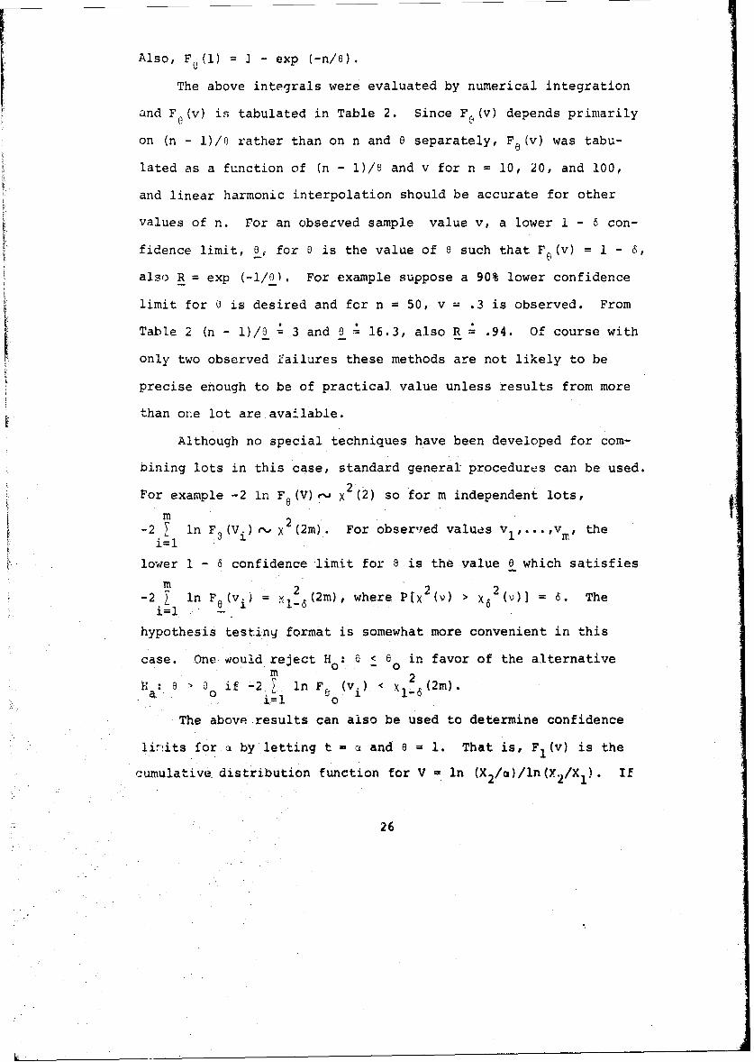
Also, F 0(1) = I - exp (-n/0).

The above integrals were evaluated by numerical integration

and F 0(v) is tabulated in Table 2. Since FIl (v) depends primarily

on (n - 1)/0 rather than on n and 0 separately, Fe (v) was tabu-

lated as a function of (n - 1)/6 and v for n = 10, 20, and 100,

and linear harmonic interpolation should be accurate for other

values of n. For an observed sample value v, a lower 1 - 6 con-

fidence limit, 0, for 0 is the value of e such that F (v) = 1 - 6,

also R = exp (-1/01. For example suppose a 90% lower confidence

limit for 0 is desired and for n = 50, v = .3 is observed. From

Table 2 (n - 1)/6 3 and e = 16.3, also R = .94. Of course with

only two observed Zailures these methods are not likely to be

precise enough to be of practical value unless results from more

than one lot are available.

Although no special techniques have been developed for com-

bining lots in this case, standard general procedures can be used.x2

For example -2 ln F (V),J X (2) so for m independent lots,m

-2 7 ln F3 (V.) ' X2(2m). For observed values vl,...,v, thei~l:

lower 1 - 6 confidence limit for a is the value 8 which satisfies

m .2 2 2-2 in (v2i 1-(2m), where P[ () > 6 = 6. The

i=l

hypothesis testing format is somewhat more convenient in this

case. One would reject H 0< 6 in favor of the alternative00m 2

H:a 6 > 60 0if "2_ ln F& (vi) < X1'6 (2m)i=l o

The above results can also be used to determine confidence

lirtits for a by letting t = a and a = 1. That is, Fl(v) is the

cumulative distribution function for V 1n (X2 / )/ln(X 2/X 1). If

26

Fl(v) = y, then1vy

P[V < v =P[a > x 2 (x/X2 ] =/

and x 2 (xl/x 2 ) v is a lower 100y% confidence limit for ,j. Proba-

bilities for this case are included in Table 2 under (n - 1)/( =

n-i.

27

6. COMPARISON OF CENSORED SAMPLING

AND COMPLETE SAMPLING

Consider a test of Ho: S < o against H : 6 > 0 at the 60 0 a 0

level of significance. A test for this hypothesis has been devel-

oped in [9] for complete samples based on the maximum likelihood

estimator, say 0. The null hypothesis is rejected if S > o o1-6'

where i satisfies P[6/s > k = y and is tabulated in [9]. The

power of the test for the alternative Sa is given by

P[/8 > (Bo /a )Z1_]. If we use the simple censored sample estiriator

the null hypothesis is rejected if b < (1/o )c (v), where v = 2nkrn

and c(v) denotes the chi-square over degrees of freedom distribu-tion [1,4]. The power is given by P[cV . (aa/o )c (a)]. Values

of v are given in Table 3 which would provide the same power for

the censored sampling test as would be obtained by using the maxi-

mum likelihood method based on a complete sample of size N. Some

combinations of r and n which would yield these values of v are

also given and the relative expected experiment time, R.E.T. =

E(Xr,n)/E(XN,N), is given in each case for 6 = 1 and a = 2. Note

that the table indicates that the comparison does not appear to

be very sensitive to the level of significance or the level of the

power being considered.

28

7. NUMERICAL EXAMPLE

Harter and Moore [6] give a simulated sample of size 40

from a Weibull population with shape parameter 2, scale parameter

100 and location parameter 10; and, they calculated maximum like-

lihood estimates based on the smallest 10, 20, 30 and 40 observa-

tions respectively. After subtracting the value of the location

parameter from each observation we calculated numerical values

which are given in Table 4 of the following quantities for

r = 2, 10, 20, 30 and 40:

v = 2nkr,n, b, $ = 1/b, ((v 2)/v)$,

23(.025) = 2 ())/(vb) = C. (V)ý, and

T(.025) = C 0 2 5 (0)8, where •(6) denotes a

lower 1 - 6 confidence limit for 3. The

lower limit based on maximum likelihood

estimates will be denoted by _m(6).

The hypothesis H 0 =o = 1 is rejected in favor of the alterna-

tive HA: • > 1 at the 8 significance level if býo < C *_() The

level of significance, V' at which this hypothesis could have been

rejected is given in Table 4. The power of a 6 level test of H against

an alternative 6a is denoted by P(6,3 a) = P[CJ < 3a Cl16(0) in

Table 4. In this example the true reliability is .90 at t = 32.46.

A conservative .9025 lower confidence limit for R, R =2 r- 1

min R(b), where R(b) = exp {-X 0 5 (2r)/2[ (X./tV+b(.025) <b<f(.025) -i"=l

(n - r + l)Wxr/t) ]), was determined for t = 32.46. For r =

20,30 and 40 the condition in t - In xr < -T/r holds so that

29

R = R(b(. 0 2 5 )). This is also the limit for r = 10 although the

above condition does not hold in this case.

The maximum likelihood estimates were included in the table

for comparison. Also confidence bounds for b and R are available

from [101 for complete sampling and from (III] 'Chapter III) or [2]

for 25% and 50% censoring and these are included. Although co..-

fidence bounds are included for the complete sample case for com-

parison purposes, it should be recalled that the efficiency of b

and the accuracy of the chi-square approximation are not as great

for large r/n. An estimate of a lower bound for reliability,

R(b), would perhaps also be a useful statistic and it is included

in the table.

30

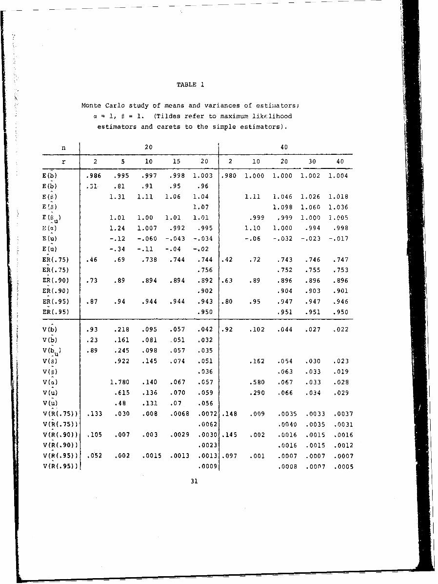
TABLE 1

Monte Carlo study of means and variances of estimaators;

a= 1, $ = 1. (Tildes refer to maximum likelihood

estimators and carets to the simple estimators).

n 20 40

r 2 5 10 15 20 2 10 20 30 40

E(b) .986 .995 .997 .998 1.003 .980 1.000 1.000 1.002 1.004

E(b) .31 .81 .91 .95 .96

E() 1.31 1.11 1.06 1.04 1.11 1.046 1.026 1.018

E(ý) 1.07 1.098 1.060 1.036

E(B) 1.01 1.00 1.01 1.01 .999 .999 1.000 1.005

E(a) 1.24 1.007 .992 .995 1.10 1.000 .994 .998

E(U) -. 12 -. 060 -. 043 -. 034 -. 06 -. 032 -. 023 -. 017

E(U) -. 34 -.11 -. 04 -. 02

ER(.75) .46 .69 .738 .744 .744 .42 .72 .743 .746 .747

ER(.75) .756 .752 .755 .753

ER(.90) .73 .89 .894 .894 .892 .63 .89 .896 .896 .896

ER(.90) .902 .904 .903 .901

ER(.95) .87 .94 .944 .944 .943 .80 .95 .947 .947 .946

ER(.95) .950 .951 .951 .950

V(b) .93 .218 .095 .057 .042 .92 .102 .044 .027 .022

V(b) .23 .161 .081 .051 .032

V(b ) .89 .245 .098 .057 .035

V(6) .922 .145 .074 .051 .162 .054 .030 .023

V(O) .036 .063 .033 .019

V(a) 1.780 .140 .067 .057 .580 .067 .033 .028

V(U) .615 .136 .070 .059 .290 .066 .034 .029

V(u) .48 .131 .07 .056

V(R(.75)) .133 .030 .008 .0068 .0072 .148 .009 .0035 .0033 .0037

V(R(.75)) .0062 .0040 .0035 .0031

V(R(.90)) .105 .007 .003 .0029 .0030 .145 .002 .0016 .0015 .0016

V(R(.90)) .0023 .0016 .0015 .0012

V(R(.95)) .052 .002 .0015 .0013 .0013 .097 .001 .0007 .0007 .0007

V(R(.95)) .0009 .0008 .0007 .0005

31

TABLE 2

Values of P[ln (X2 /t)/ln (X2 /X1 ) < v], 6 = (c/t)8 - -1/in R.

n = 10

n-i

Iiv1 2 3 4 5 6 7 8 9

-30.0 .006 .015 .024 .032 .038 .043 .047 .051 .055

-20.0 .009 .023 .036 .047 .056 .063 .070 .075 .080

-10.0 .017 .044 .069 .090 .107 .122 .134 .144 .153

- 9.0 .018 .049 .076 .100 .118 .134 .147 .158 .168

- 8,0 .020 .054 .085 .111 .132 .149 .163 .176 .187

- 7.0 .023 .061 .096 .125 .149 .168 .184 .198 .210

- 6.0 .027 .070 .111 .144 .170 .192 .210 .226 .239- 5.0 .031 .083 .130 .168 .199 .225 .246 .263 .279

- 4.0 .038 .101 .157 .204 .240 .270 .295 .316 .334- 3.5 .043 .113 .176 .227 .268 .301 .328 .350 .370

- 3.0 .049 .128 .200 .257 .302 .339 .368 .393 .414

- 2.5 .057 .149 .230 .296 .347 .387 .420 .448 .471

- 2.0 .068 .177 .272 .348 .406 .4s2 .489 .519 .544

- 1.5 .084 .217 .332 .421 .489 .540 .581 .614 .641

- 1.0 .111 .281 .424 .531 .609 .666 .709 .743 .769

- 0.5 .161 .396 .579 .704 .787 .842 .879 .905 .923

- 0.3 .196 .469 .669 .796 .872 .918 .945 .963 .974

- 0.1 .248 .566 .773 .887 .945 .974 .987 .994 .997

0.0 .284 .622 .823 .923 .967 .987 .995 .998 .999

0.1 .328 .678 .864 .946 .979 .992 .997 .999 1.000

0.3 .427 .766 .913 .969 .989 .996 .999 1.000

0.6 .557 .842 .946 .982 .994 .998 .999

1.0 .671 .892 .964 .988 .996 .999 1.000

32

TABLE 2 (continued)

n =20

n-1

v1 2 3 4 5 6 7 8 9 19

-30.0 .006 .015 .024 .032 .038 .044 .048 .052 .056 .086

-20.0 .008 .022 .036 .047 .057 .064 .071 .077 .082 .121

-10.0 .016 .043 .069 .091 .109 .123 .136 .147 .156 .21ý

- 9.0 .018 .048 .076 .100 .120 .136 .150 .161 .172 .237

- 8.0 .020 .053 .085 .111 .133 .151 .166 .179 .190 .262

- 7.0 .022 .060 .096 .126 .150 .170 .187 .201 .214 .291

- 6.0 .026 .069 .110 .144 .172 .195 .214 .230 .244 .329

- 5.0 .030 .082 .±29 .169 .201 .228 .249 .268 .284 .379

- 4.0 .037 .099 .157 .204 .242 .273 .299 .321 .339 .446

- 3.5 .042 .111 .175 .228 .270 .304 .332 .356 .376 .489

- 3.0 .047 .126 .199 .257 .304 .342 .373 .399 .421 .541

- 2.5 .055 .146 .229 .296 .349 .391 .425 .453 .477 .605

- 2.0 .066 .173 .270 .348 .408 .455 .493 .524 .550 .684

- ].5 .082 .213 .330 .421 .490 .544 .585 .619 .646 .780

- 1.0 .107 .276 .420 .529 .609 .668 .713 .747 .774 .890

- 0.5 .155 .388 .572 .700 .785 .842 .880 .906 .925 .983

- 0.3 .189 .459 .661 .790 .869 .916 .945 .963 .974 .998

- 0.1 .239 .553 .763 .881 .941 .972 .986 .993 .997 1.000

0.0 .274 .608 .812 .916 .964 .985 .994 .997 .999

0.1 .316 .662 .852 .939 .976 .991 .996 .999 1.000

0.3 .412 .749 .902 .963 .986 .995 .998 .999

0.6 .538 .826 .937 .977 .992 .997 .999 1.000

1.0 .651 .878 .957 .985 .995 .998 .999

33

TABLE 2 (continued)

n = 100

n-i

v1 2 3 4 5 6 7 9 19 99

-30.0 .005 .015 .024 .032 .039 .044 .049 .057 .088 .150

-20.0 .008 .022 .036 .047 .057 .065 .072 .084 .123 .204

-10.0 .016 .043 .069 .091 .109 .125 .138 .159 .222 .347

- 9.0 .017 .047 .076 .100 .120 .137 .151 .174 .242 .375

- 8.0 .019 .053 .085 .112 .134 .153 .168 .193 .266 .408

- 7.0 .022 .060 .095 .126 .151 .172 .189 .217 .297 .4496.0 .025 .068 .110 .144 173 .197 .216 .248 .335 .4985.0 .030 .081 .129 .169 .202 .230 .252 .2P8 .385 .560

- 4.0 .036 .098 .156 .204 .244 .276 .302 .344 .452 .638

- 3.5 .041 .110 .174 .228 .271 .306 .335 .380 .496 .685

- 3.0 .046 .125 .197 .258 .306 .345 .376 .425 .548 .739

- 2.5 .054 .144 .228 .296 .350 .394 .429 .482 .612 .798

- 2.0 .064 .171 .269 .348 .409 .458 .497 .555 .690 .863

- 1.5 .079 .210 .327 .420 .491 .546 .589 .651 .785 .927

- 1.0 .104 .272 .417 .528 .609 .670 .715 .777 .893 .979

- 0.5 .151 .381 .567 .697 .784 .841 .880 .926 .983 .999

- 0.3 .184 .451 .654 .786 .867 .915 .945 .974 .998 1.000

- 0.1 .233 .543 .755 .875 .938 .970 .985 .997 1.000

0.0 .266 .597 .803 .910 .960 .983 .993 .F99

0.1 .307 .650 .843 .934 .973 .989 .996 .999

0.3 .400 .736 .893 .958 .984 .994 .998 1.000

0.6 .524 .813 .929 .974 .990 .996 .999

1.0 .636 .867 .952 .982 .994 .998 .999

3A

lilt

TABLE 3

Comparison between maximum likelihood test (complete

sample) and simple censored sample test.

N a 8/80 Power v n 15 20 30 60 100a 0 _75 2_____1__4____

10 .10 1.73 .75 28 r 12 13 14 14 14

10 .10 2.00 .90 28 r 12 13 14 14 14

10 .05 2.25 .90 28 r 12 13 14 14 14

R.E.T. (8=1) .51. .34 .21 .09 .05

R.E.T. (8=2) .72 .59 .46 .30 .23

20 .05 1.73 .90 591 r 23 27 29

20 .05 1.83 .95 601 r 23 27 29

R.E.T. (8=1) .39 .16 .09

R.E.T. (8=2) .63 .41 .31

35

TABLE 4

Numerical example, n = 40, 8 = 2, a = 100.

r v b b a a au u P(.025) 8m(.025) T.025) TItI(.025)

2 2.03 .68 .34 1.46 2.90 .04 5.36

10 19.30 .81 .73 1.24 1.37 1.11 .58 2.13

20 44.68 .48 .48 2.08 2.09 1.99 1.90 1.31 1.19 3.02 2.92

30 78.50 .58 .56 1.73 1.78 1.69 1.68 1.23 1.18 2.31 2.36

40 159.21 .53 .51 1.88 1.95 1.86 1.88 1.49 1.45 2.32 2.41

r ri R(32.46) R(32.46) R RM R(b) 6' P(.025,1.5) P(.025,2.0)

2 76.5 27.9 .75 .64

10 151.3 136.6 .86 .87 .73 .79 .30 .19 .47

20 83.9 83.8 .87 .87 .72 .79 .82 .005 .43 .88

30 96.4 96.3 .86 .87 .72 .79 .82 .001 .68 .99

40 92.2 92.8 .87 .88 .75 .82 .84 <.001 .95 >.999

36

REFERENCES

[11 Beyer, W. H. (Editor), Handbook of Tables for Probabilityand Statistics, Second Edition. Cleveland Ohio: The Chem-ical Rubber Co., 1968.

[2] Billman, B. R.; Antle, C. E.; and Bain, L. J., "Statisticalinference from censored Weibull data", submitted toTechnometrics.

[3] Cohen, A. C. Jr., "Maximum likelihood estimation in theWeibull distribution based on complete and on censoredsamples", Technometrics, 7 (1964), 579-588.

[4] Guenther, W. C., Concepts of Statistical Inference. McGraw-Hill Book Co. (1965).

[5] Harter, H. L. and Moore, A. H., "Maximum likelihoc•. estima-tion, from doubly censored samples, of the parameters of thefirst asymptotic distribution of extreme values", Journal ofthe American Statistical Association, 63 (1968), 889-901.

[6] Harter, H. L. and Moore, A. H., "Maximum-Likelihood Estima-tion of the Parameters of Gamma and Weibull Populations fromComplete and Censored Samples", Technometrics, 7 (1965),639-643.

[7] Jaech, j. L., "Estimation of Weibull distribution shape para-meter when no more than two failures occur per lot",Technometrics, 6 (1964), 415-422.

[8] Mann, N. R.: Fertig, K. W.; and Scheuer, E. M., Confidenceand Tolerance Bounds and a New Goodness-of-Fit Test for Two-Parameter Weibull or Extreme-Value Distributions . ARL 71-0077,Aerospace Research Laboratories, Wright-Patterson Air ForceBase, Ohio. (1971).

19] Thoman, D. R.; Bain, L. J." and Antle, C. E., "Inferences onthe parameters of the Weibull distribution", Technometrics,11 (1969), 445-460.

[101 Thoman,*D. R.; Bain, L. J.; and Antle, C. E., "Maximum likeli-hood estimation, exact confidence intervals for reliabilityand tolerance limits in the Weibull distribution", Technometrics,12 (1970), 363-372. [For summary and additional tables, seeAppendix A.1 of Bain, Lee J. and Antle, Charles E., InferentialProcedures for the Weibull and Generalized Gamma Distributions,ARL 70-0266, Aerospace Research Labs., Wright-Patterson AFB.(1970), AD718103.]

111] White, John S., The Moments of Log-Weibull Order Statistics,General Motors Research Publication GMR-717, General MotcrsCorporation, Warren, Michigan (1967).

37

CHAPTER III

RESULTS FOR CENSORED SAMPLING BASED

ON THE MAXIMUM LIKELIHOOD ESTIMATORS

1. INTRODUCTION AND NOTATION

In life testing experiments it is a fairly common practice

to terminate the experiment before all items have failed. The

Weibull distribution is often used as a model for the observa-

tions and when a computer is available maximum likelihood esti-

mation of the parameters is to be recommended. The tables pre-

sented in this paper enable one to set confidence limits on the

parameters and the reliability based on the maximum likelihood

estimates for selected censoring &," sample sizes.

It is also observed that, as in the case with no censoring,

the maximum likelihood estimator of the reliability is very nearly

unbiased and its variance is near the Cram~r-Rao lower bound.

Unbiasing factors for .he raximum likelihood estimator of the

shape parameter aie given.

The forn, of the Weibull distribution function considered in

this chF.nter is

F(t;b,c) 1- ! - exp (-ft/b) ) for t > 0

where b is the scale parameter and c is the shape parameter The

38

reliability at time t is simply R(t) = exp (-(t/b)C).

Let b and c be the maximum likelihood estimators of b and c

and let R(t) be the maximum likelihood estimator of R(t). Then

it is known [1,5] that the distribution of c/c and c log (b/b)

does not depend upon b and c, although it will, of course, depend

upon the sample size, n, and the number of observations before

censoring, r. Thus for a given n and r these pivotal functions

can be used to test hypotheses about b and c or set confidence

intervals on b and c. The tables required when there is no cen-

soring are given by Thoman, Bain and Antle [4], and this paper

presents the tables when either 25% or 50% of the largest obsex-

vations are censored. Moreover, it appears that linear interpo-

lation should be adequate for censoring levels between those

given in the tables.

It was shown [51 that the distribution of R(t) depends only

upon the valuesof R(t), n and r. Tables providing lower confidence

limits for R(t) based upon m.l.e.'s from complete samples are

given by Thoman, Bain and Antle [5], and this paper presents the

tables needed when either 25% or 50% of the sample values are

censored from above.

The values for each n were obtained by simulation with 8000

samples (of size n) used for n = 40, 60, 80, 100 and 120. The

8000 samples were run in two sets of 4000 and the critical values

for each set of 4000 were compared. The critical values for the

reliability tables for R(t) , .9 usually differed by less than

.004, and so we believe there is little sampling error in these

tables. The critical values for the other tables differed somewhat

39

more, those for y's of .05, .1, .9 and .95 usually differed by

about .02.

2. Inferences on the Parameters

2.1 Inferences on the shape parameter

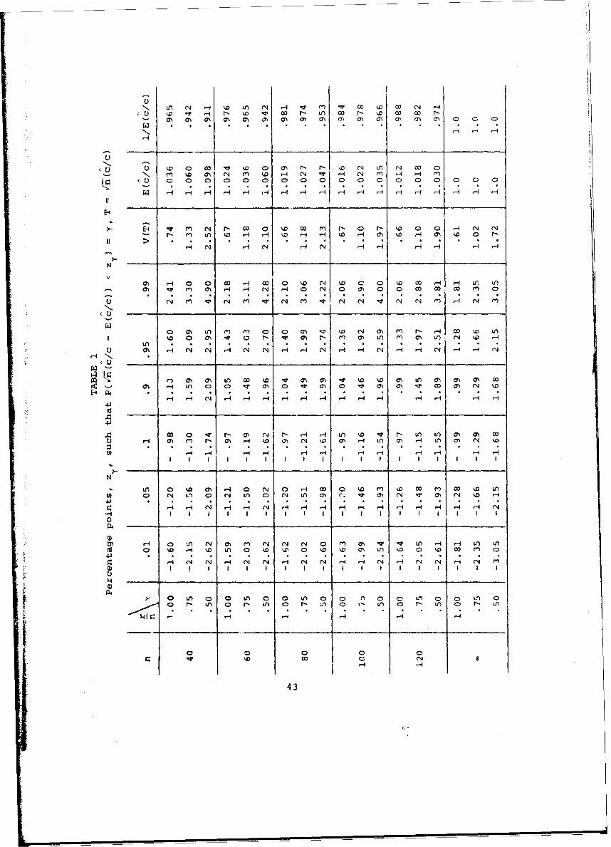
The standardized function V/ (c/c - E(c/c)) was considered

in this case because of the convenience in the use of the asymp-

totic values and for better interpolation in the table. Table 1

gives percentage points for this quantity for selected cumulative

probability levels. The asymptotic percentage points were ob-

tained from the work of Harter and Moore [2] and are also included

in the table. It is seen from the table that the asymptotic

values are approached quite slowly. We believe this is due to

the lack of symmetry when the samples are censored on one side,

and it appears that the asymptotic values are not very useful in

the censored case. Unbiasing factors for c are included in Table 1.

Tests of hypotheses concerning c or confidence intervals for

c based on the function /n (c/c - E(c/c.) can be easily developed

with the aid of Table 1. For example a 1 - a confidence interval

for c is given by

(c/(E(c/c) + z l_/ 2/1 n),c/(E(c/c) + z /2//)],

where the z and E(c/c) are given in Table 1.

Y

2.2 Inferences on the scale paramecer

Again as an aid in interpolation, percentage points for the

expression Vn c in (b/b) are given in Table 2. Interpolation

40

should be fairly good, but as was true for the shape parameter it

appears that the approach to the asymptotic values is quite slow,

and for one sided censored samples with n less than 120 the asymp-

totic values should not be used. In this case, for example, a

100(1 - a)% confidence interval for b is given by[b exp (-ul_•/2/./c), b exp (-u/2/).

1-a~/2 cz/2/n)

3. Inferences on the Reliability

In many studies in which the Weibull distribution is used as

a model, the primary interest is in the reliability at some time

t, R(t). It is fortunate that in spite of skewness, censoring

and other difficulties, the m.l.e. of R(t) for reasonable values

of R(t) has negligible bias and its variance is very close to

the Cramdr-Rao lower bound for the variance of an unbiased estima-

tor of R(t). This property was noted in [5) for complete sampling,

and it also holds for censored sampling. The bias of R(t) is

given in Table 3 and the variance in Table 4. A comparison of

the variances and the Cram~r-Rao lower bounds is given in Table 5.

Table 6 gives lower confidence limits on R(t). These are

read directly from the table by entering the value of R(t) ob-

served. A need for these tables to include high reliability

levels has been communicated to the authors, and this accounts

for the number of entries for reliabilities near 1 in the tables.

4. Example

Harter and Moore [3] give a simulated sample of size 40 from

a Weibull population with shape parameter 2, scale parameter 100

41

and location parameter 10; and, they calculated maximum likelihood

estimates based on the smallest 10, 20, 30 and 40 observations,

respectively. This example with the location parameter assumed

known may be used to illustrate the use of the tables.

For r = 20, c = 2.091 and b = 83.8. The unbiased estimate

of c is (.911)(2.091) = 1.90. Also for example, a test of

H c = 1 against the alternative HA: c > 1 corresponds to a test0 A

of whether an exponential model is appropriate, or whether a

Weibull model with an increasing failure rate is needed. This

hypothesis is rejected at the .05 level if /40 (c/l - 1.098) > 2.95,

or if c > 1.56. Thus the hypothesis is rejected. A 90% confi-

dence interval for c is given by

[2.091/(1.098 + 2.95/4--O), 2.091/(1.098 - 2.09//1 )]

= [1.34, 2.721.

A 90% confidence interval for b is

[83.8 exp (-2.16/(2.091)/40), 83.8 exp (3.75/(2.091)V/4) ]

= [71.17, 111.27].

In this example the true reliability at t = 32.459 is .90.

2091The m.l.e. for r = 20 is R = exp (-(32.459/83.8)2"9) = .871.

From Table 6 a lower 90% confidence limit for R(t) is .80.

42

N LA) N Hq 'D LI (N H- (n " ) OD ýD 0 N H-1 'r- ý1 Hc N0 r- LO N0 LA Co N0 00D C

o 0 a' 0 a< w< C< m r- 7D oN dn N~ 0 o~wN H) N H1 - N T -

'N

mU 0 0 0 0 0- c 0 %0 0N w c C0 ý 0 0 H 1- 0r 0

m ~ N m N r- 0- N~ r-4 0 NN a m 0 00 HD OD N

o a%< Ln m H HD <0 Ch H 10 H1 0< m. H- r- 0~, <0 %0 N

HN N H- N N H H N H- -A C H H; H4 Hý Hý

n _)m_____I* (_) W ý k n 7 ) N c

0% H4 0 0 0 H Ch 0 .T ON <0 V 0N 0) -Vl HD H) N w

co 0~ -q H- H N H -0 1 N n 0 1 IT< r- 0 n in m. ) 0o

q ON m" - aN C") o N) N w N) N- n N) N- C) H (N w

o LAA ' " 0 00 0') -4 o N 0' 1-4 N H Cfl w. m U') o D0 N. 0I 0' N n ND N' 0i N) (1) 0v m C") 0' 0L N .0 H4

04.

1- 0 Ln N m Om N (N H H LA0,~ LA HA 0') 0L O

aA 0n 0 0') H 0 ND t ) 0 <0 C) .0 0n 0I C) <.0

00

H o A N 0') N N n") 0')~ ' LA H A o

'U < H <. L 0 '.o <o 0 .o <. 0) L < 0 <. 43

TABLE 2

Percentage points, u, such that P(/nc ln(b/b) u U ) = y

n y .01 .05 .1 .9 .95 .99

1.00 -2.58 -1.82 -1.41 1.39 1.80 2.62

40 .75 -3.29 -2.25 -1.69 1.39 1.85 2.61

.50 -6.21 -3.77 -2.91 1.63 2.16 2.96

1.00 -2.48 -1.78 -1.38 1.37 1.77 2.56

60 .75 -3.22 -2.16 -1.68 1.,i2 1.84 2.66

.50 -5.37 -3.56 -2.69 1.67 2.18 3.01

1.00 -2.51 -1.76 -1.37 1.37 1.76 2.49

80 .75 -3.11 -2.10 -1.61 1.43 1.85 2.65

.50 -5.14 -3.45 -2.62 1.71 2.16 3.08

1.00 -2.45 -1.74 -1.37 1.35 1.73 2.50

100 .75 -3.12 -2.09 -1.60 1.44 1.85 2.61

.50 -4.92 -3.34 -2.49 1.78 2.26 3.19

1.00 -2.44 -1.73 -1.35 1.35 1.74 2.48

120 .75 -3.01 -2.01 -1.58 1.45 1.86 2.63

.50 -4.50 -3.17 -2.44 1.75 2.27 3.13

1.00 -2.45 -1.73 -1.35 1.35 1.73 2.45

.75 -2.69 -1.90 -1.48 1.48 1.90 2.69

.50 -3.69 -2.61 -2.03 2.03 2.61 3.69

44

TABLE 3 BIAS IN R(t)-

25% Censoring 50% Censoring

R(t) 40 60 80 100 120 40 60 80 100 120

.75 .005 .003 .003 .001 .002 .002 .000 .001 .000 .000

.80 .005 .003 .003 .002 .002 .004 .002 .002 .001 .001

.85 .004 .002 .003 .001 .001 .005 .002 .002 .001 .002

.90 .003 .001 .002 .001 .001 .004 .002 .002 .001 .001

.925 .002 .000 .001 .000 .001 .003 .001 .002 .001 .001

.95 .001 .000 .001 .000 .000 .001 .001 .001 .001 .001

.96 .000 -. 000 .000 -. 000 .000 .001 .000 .001 .000 .000

.97 -. 000 -. 000 .000 -. 000 -. 000 .000 .000 .000 .000 .000

.98 -. 000 -. 000 -. 000 -. 000 -. 000 -. 000 -. 000 -. 000 -. 000 -. 000

.99 -.000 -.000 -.000 -.000 -.000 -.000 -.000 -.000 -.000 -.000

.905 -. 001 -. 000 -. 000 -. 000 -. 000 -. 001 -. 000 -. 000 -. 000 -. 000

.996 -. 001 -. 000 -. 000 -. 000 -. 000 -. 001 -. 000 -. 000 -. 000 -. 000

.997 -. 000 -. 000 -. 000 -. 000 -. 000 -. 001 -. 000 -. 000 -. 000 -. 000

.998 -. 000 -. 000 -. 000 -. 000 -. 00uu -. 001 -. 000 -. 000 -. 000 -. 000

.999 -. 000 -. 000 -. 000 -. 000 -. 000 -. 000 -. 000 -. 000 -. 000 -. 000

45

^I

TABLE 4 VARIANCE OF R(t)

25% Censoring 50% Censoring

R(t) n 40 60 80 100 120 40 60 80 100 120

.75 .0035 .0023 .0018 .0013 .0012 .0040 .0024 .0019 .0014 .0013

.80 .0030 .0019 .0015 .0011 .0010 .0032 .0020 .0016 .0012 .0011

.85 .0023 .0015 .0012 .0009 .0008 .0025 .0016 .0013 .0010 .0008

.90 .0015 .0010 .0008 .0006 .0006 .0016 .0011 .0009 .0007 .0006

.925 .0011 .0008 .0006 .0005 .0004 .0012 .0008 .0007 .0005 .0005

.95 .0007 .0005 .0004 .0003 .0003 .0008 .0006 .0004 .0004 .0003

.96 .0005 .0004 .0003 .0003 .0002 .0006 .0004 .0004 .0003 .0003

•97 .0004 .0003 .0003 .0002 .0002 .0005 .0003 .0003 .0003 .0002

.98 .0003 .0002 .0002 .0002 .0002 .0003 .0002 .0002 .0002 .0002

.99 .0002 .0002 .0001 .0001 .0001 .0002 .0002 .0002 .0001 .0001

.995 .0001 .0001 .0001 .0001 .0001 .0001 .0001 .0001 .0001 .0001

.996 .0001 .0001 .0001 .0001 .0001 .0001 .0001 .OC01 .0001 .0001

.997 .0001 .0001 .0001 .0001 .0001 .0001 .0001 .0001 .0001 .0001

.998 .0001 .0001 .0001 .0001 .0001 .0001 .0001 .0001 .0001 .0001

.999 .0001 .0001 .0001 .0001 .0001 .0001 .0001 .0001 .0001 .0001

46

Ii

TABLE 5 COMPARISON OF V(R(t)) WITH CRLB VARIANCE x 10 (n = 40)

R(t) .75 .80 .85 .90 .925 .95 .96 .97 .98 .99 >.99

r= 30

V(R(t)) 35 30 23 15 i.1 07 05 04 03 02 01

CRLB 33 28 22 14 10 06 04 03 02 01 01

r = 20

V(R(t)) 40 32 25 16 12 08 06 05 03 02 01

CRLB 35 29 23 16 12 07 05 04 02 01 01

47

TABLE 6 A

90% LOWER CONFIDENCE LIMITS ON R(t)

25% CENSORING 50% CENSORING

R(t) n 40 60 80 100 120 40 60 80 100 120

.70 .623 .638 .641 .650 .654 .616 .639 .644 .652 .655

.72 .641 .657 .661 .669 .673 .635 .658 .663 .672 .674

.74 .659 .676 .681 .690 .693 .653 .677 .683 .691 .694

.76 .678 .696 .702 .710 .713 .674 .696 .703 .711 .714

.78 .698 .716 .723 .731 .734 .694 .716 .723 .732 .734

.80 .718 .737 .744 .752 .755 .715 .736 .744 .752 .755

.82 .739 .758 .766 .774 .776 .737 .757 .765 .773 .776

.84 .761 .780 .789 .796 .798 .759 .779 .787 .795 .797

.86 .783 .802 .810 .818 .821 .783 .801 .810 .817 .819

.88 .807 .826 .833 .841 .843 .807 .824 .832 .839 .842

.90 .832 .850 .857 .864 .866 .832 .847 .855 .862 .864

.92 .858 .875 .882 .888 .890 .858 .872 .879 .886 .888

.94 .886 .901 .907 .913 .914 .886 .898 .904 .910 .912

.95 .901 .915 .920 .925 .927 .901 .911 .917 .922 .924

.96 .917 .929 .934 .939 .940 .917 .925 .930 .935 .937

.97 .938 .943 .947 .952 .953 .933 .940 .944 .949 .951

.98 .951 .959 .963 .966 .967 .951 .956 .959 .964 .965

.99 .971 .976 .979 .981 .982 .971 .974 .977 .979 .980

.9925 .977 .981 .984 .986 .986 .977 .979 .982 .984 .985

.995 .983 .987 .989 .990 .990 .983 .985 .987 .988 .989

.996 .986 .989 .990 .992 .992 .986 .987 .989 .990 .991

.997 .989 .992 .993 .994 .994 .989 .989 .991 .992 .993

.998 .992 .073 .995 .995 .996 .992 .992 .994 .995 .995

.9985 .993 .995 .996 .996 .997 .993 .994 .995 .996 -996

.999 .994 .996 .997 .998 .998 .994 .995 .996 .997 .99748

TABLE 6B

95% LOWER CONFIDENCE LIMITS ON R(t)

25% CENSORING 50% CENSORING

R(t) n 40 60 80 100 120 40 60 80 100 120

.70 .594 .626 .624 .62S .643 .600 .623 .628 .639 .646

.72 .613 .644 .643 .647 .662 .614 .641 .647 .659 .664

.74 .632 .662 .664 .669 .681 .632 .660 .667 .678 .683

.76 .651 .680 .684 .691 .701 .651 .679 .686 .698 .702

.78 .671 .699 .705 .713 .722 .671 .699 .707 .719 .722

.80 .692 .719 .726 .736 .743 .691 .719 .727 .741 .742

.82 .714 .740 .748 .759 .764 .712 .740 .749 .761 .762

.84 .737 .761 .771 .782 .786 .734 .761 .771 .782 .784

.86 .760 .784 .795 .806 .809 .757 .784 .793 .805 .806

".88 .785 .808 .819 .830 .832 .781 .807 .817 .827 .829

.90 .811 .833 .844 .854 .856 .807 .831 .841 .851 .852

.92 .839 .860 .870 .879 .881 .834 .857 .866 .876 .877

.94 .869 .888 .897 .904 .906 .863 .883 .892 .902 .903

.95 .885 .903 .911 .917 .920 .878 .879 .906 .915 .917

.96 .902 .:19 .926 .932 .933 .894 .913 .920 .929 .931

.97 .920 .935 .941 .946 .948 .913 .929 .936 .946 .947

.98 .940. .953 .957 .962 .963 .933 .947 .952 .960 .961

.99 .964 .972 .976 .978 .979 .957 .968 .971 .975 .977

.9925 .J70 .978 .981 .993 .984 .965 .974 .977 .980 .981

.995 .978 .984 .986 .988 .988 .973 .980 .983 .985 .986

.996 .981 .986 .988 .990 .990 .976 .983 .985 .988 .989

.997 985 .989 .991 .992 .992 .980 .986 .988 .990 .991

.998 .988 .992 .993 .994 .995 .985 .990 .992 .993 .994

.9985 .991 .994 .995 .996 .996 .987 .992 .993 .994 .995

.999 .993 .995 .996 .997 .997 .990 .994 .995 .996 .996

49

I

TABLE 6C

98% LOWER CONFIDENCE LIMITS ON R(t)

25% CENSORING 50% CENSORING

I(t) n 40 60 80 100 120 40 60 80 100 120

.70 .571 .5 - .610 .622 .625 .590 .606 .613 .628 .631

.72 .589 .615 .629 .641 .C45 .606 .623 .632 .647 .649

.74 .601 .635 .648 .661 .666 .622 .641 .650 .665 .669

.76 .627 .654 .668 .681 .687 .639 .660 .67P .685 .689

.78 .647 .675 .688 .702 .708 .657 .679 .689 .704 .708

.80 .669 .696 .709 .723 .730 .676 .698 .710 .725 .729

.82 .690 .718 .731 .745 .752 .695 .719 .731 .746 .754

.84 .713 .741 .753 .768 .775 .716 .740 .752 .768 .773

.Su .737 .764 .777 .791 .798 .737 .763 .775 .790 .792

.88 .763 .789 .801 .815 .822 .760 .786 .799 .813 .819

.90 .790 .816 .827 .840 .846 .785 .811 .824 .837 .848

.92 .819 .844 .854 .866 .871 .812 .838 .850 .863 .871

.94 .851 .873 .883 .893 .896 .842 .866 .877 .889 .893

.95 .868 .889 .898 .908 .911 .858 .881 .892 .903 .906

F .96 .886 .906 .914 .923 .926 .875 .897 .907 .918 .922

.97 .906 .924 .931 .938 .941 .895 .915 .924 .934 .937

.98 .928 .943 .950 .955 .957 .917 .935 .943 .951 .953

.99 .954 .966 .970 .974 .976 .945 .959 .964 .971 .972

.9925 .962 .972 .976 .980 .981 .953 .966 .970 .976 .978

.995 .971 .979 .983 .985 .986 .963 .974 .977 .982 .984

.996 .975 .983 .985 .988 .989 .967 .978 .981 .985 .987

.997 .979 .986 .988 .990 .991 .972 .982 .984 .988 .989

.998 .984 .990 .991 .993 .994 .978 .986 .988 .991 .992

.9985 .987 .992 .993 .994 .995 .982 .989 .990 .993 .994

.999 .990 .994 .995 .996 .996 .986 .992 .993 .995 .995

5o

T7.BLE 6D

99% LOWER CONFIDELCE LIMITS ON R(t)

25% CENSORING 50% CENSORING

R(t) n 40 60 80 100 120 40 60 80 100 120

.70 .555 .585 .601 .618 .623 .566 .590 .609 .613 .615

.72 .574 .603 .620 .636 .641 .582 .60/ .626 .633 .636

.74 .592 .622 .638 .655 .661 .599 .624 .643 .652 .656

.76 .612 .642 .658 .674 .680 .617 .643 .661 .672 .677

.78 .632 .662 .678 .694 .701 .636 .662 .679 .693 .698

.80 .652 .684 .699 .715 .721 .655 Eel .698 .714 .720

.82 .674 .705 .720 .736 .743 .675 .702 .718 .735 .742

.84 .697 .728 .743 .759 .765 .696 .723 .739 .758 .765

.86 .722 .752 .766 .782 .788 718 .746 .761 .780 .788

.88 .747 .777 .791 .806 .812 .742 .770 .784 .804 .812

.90 .775 .804 .816 .831 .837 .768 .796 .809 .829 .836

.92 .803 .832 .844 .858 .863 .795 .823 .836 .854 .861

.94 .838 .863 .873 .886 .890 .826 .853 .865 .881 .886

.95 .855 .879 .889 .901 .905 .843 .869 .881 .895 .899

.96 .874 .896 .906 .916 .920 .861 .886 .897 .910 .914

.97 .895 .915 .923 .933 .936 .881 .905 .915 .927 .931

.98 .918 .936 .943 .951 .954 .904 .926 .935 .945 .949

.99 .947 .960 .966 .971 .973 .934 .953 .959 .965 .967

.9925 .956 .968 .973 .977 .978 .943 .960 .966 .971 .974

.995 .966 .975 .980 .984 .984 .954 .969 .977 .978 .982

.996 .970 .979 .983 .986 .987 .959 .973 .978 .981 .985

.997 .975 .983 .986 .989 .989 .966 .v77 .982 .985 .988

.998 .981 .987 .990 .992 .992 .974 .982 .986 .988 .991

.9985 .984 .990 .992 .993 .994 .978 .975 .988 .991 .993

.999 .987 .992 .994 .995 .996 .983 .988 .991 .993 .994

51

REFERENCES

[1] Antle, C. E., and Bain, L. J., "A property of maximum like-lihood estimators of location and scale parameters", SIAMReview, 11 (1969), 251-253.

[2] Harter, H. L.; Moore, A. H., "Asymptotic variances and co-variances of maximum likelihood estimators, from censoredsamples, of the parameters of Weihull and Gamma population",Annals of Mathematical Statistics, 38 (1967), 557-570.

[3] Harter, H. L.; Moore, A. H., "Maximum likelihood estimationof the parameters of Gamma and Weibull populations from com-plete and from censored samples", Technoinetrics, 7 (1965),639-643.

[4] Thoman, D. R.; Bain, L. J. and Antle, C. E., "Inferences onthe parameters of the Weibull distribution", Technometrics,11 (1969), 445-460.

[5] Thoman, D. R.; Bain, L. J. and Antie, C. E., "Maximum like-lihood estimation, exact confidence intervals for reliabilityand tolerance limits in the Weibull distribution", Technometrics,12 (1970), 363-372. [For summary and additional taes, seeAppendix A.1 of Bain, Lee J. and Antle, Charles E., InferentialProcedures for the Weibull and Generalized Gamma Distributions,ARL 70-0266, Aerospace Research Labs., Wright-Patterson AFB.(1970), AD 718103.]

52