aerostructural optimization of the common research model ... · of the aerostructural solution with...
TRANSCRIPT

Aerostructural optimization of the Common Research Modelconfiguration
Gaetan K.W. Kenway,∗
Joaquim R. R. A. Martins†
University of Michigan, Department of Aerospace Engineering, Ann Arbor, MI Graeme J. Kennedy, ‡
Georgia Institute of Technology, School of Aerospace Engineering, Atlanta, GA
The NASA Common Research Model (CRM) has become a standard test case for verification and validation of Reynolds averaged Navier–Stokes computational fluid dynamics codes. In this paper we evaluate the suitability of the CRM for aerostructural and aeroelastic optimization studies. Since the CRM was originally intended for aerodynamic studies only, the undeformed geometry is not available. To address this issue, we designed a jig shape and the corresponding wingbox structure for the CRM using an inverse design procedure. The results are verified by computing the drag coefficient of the aerostructural solution with the jig shape at the nominal CRM operating conditions. The drag differs by less than one drag count relative to the CRM original shape. Using the CRM jig geometry, a sample high-fidelity aerostructural optimization is performed to determine the potential decrease in fuel burn for a long-range design mission when varying wing planform and airfoil shapes. The optimization increases the aspect ratio of the wing from 9.0 to 12.6 and reduces the fuel burn by 8.8%. We also perform a series of gust load analysis on both the initial and optimized designs and determine that the optimized structure is critical under gust loads. The aerostructural optimization produces a high aspect ratio wing with effective passive aeroelastic tailoring, but additional load cases with cruise-like lift distributions are required to produce a more realistic wing design.
I. Introduction Numerical analysis techniques for the simulation of complex physical systems have transformed the way design
engineers analyze and evaluate new designs. While parameter studies and carpet plots have been used long before the advent of numerical methods, automated numerical analysis has greatly increased the efficiency of their generation. Carpet plots and parameter studies can be helpful in understanding the influence of key parameters in a low dimen-sionality design space, but these graphical methods become difficult to handle as the number of parameters increases. With numerical analysis, the natural extension of 1 and 2 dimensional studies is numerical optimization—a systemic and automatic approach to improving a desired characteristic of a system of interest.
Numerical optimization has the potential to be a powerful tool that can complement more traditional design methodologies. Optimization using high-fidelity, physics-based models such as computational fluid dynamics (CFD) and computational structural mechanics (CSM) are especially promising, as they can handle new aircraft configu-rations for which model calibrations are not known. By capturing the relevant physics of the underlying physical process, optimization improvements predicted by the numerical analysis are more likely to realized in the real world. Equivalently, good optimization algorithms invariably exploit any shortcoming in the numerical model left by missing physical constraints.
An example of how missing physics in an optimization problem can be seen in previous optimization results by the authors [1]. In that work, multipoint optimization problems were solved with fuel burn and take-off gross weight (TOGW) as the objective functions. The TOGW objective favored designs with lower structural weight at the expense of higher drag. As a result, the optimized airfoil cross sections became excessively thick, approaching a 15% t/c near the wing break, and required very rapid pressure recovery towards the trailing edge. These thick cross sections resulted in a substantial reduction of the wingbox mass. However, since the solution of the Euler equations cannot predict flow separation, when the optimized design were analysed using Reynolds-averaged Navier–Stokes (RANS) CFD, the optimized design actually performed worse than the initial design: The thick cross sections exhibited strong shocks, leading to shock induced flow separation. In this case, since the optimizer is missing the critical information
∗Post Doctoral Research Fellow †Associate Professor, AIAA Senior Member ‡Assistant Processor
1 of 19
American Institute of Aeronautics and Astronautics
Dow
nloa
ded
by N
ASA
LA
NG
LE
Y R
ESE
AR
CH
CE
NT
RE
on
Janu
ary
30, 2
018
| http
://ar
c.ai
aa.o
rg |
DO
I: 1
0.25
14/6
.201
4-32
74
15th AIAA/ISSMO Multidisciplinary Analysis and Optimization Conference
16-20 June 2014, Atlanta, GA
10.2514/6.2014-3274
Copyright © 2014 by the authors.
Published by the American Institute of Aeronautics and Astronautics, Inc., with permission.
AIAA AVIATION Forum
Dow
nloa
ded
by N
ASA
LA
NG
LE
Y R
ESE
AR
CH
CE
NT
RE
on
Janu
ary
30, 2
018
| http
://ar
c.ai
aa.o
rg |
DO
I: 1
0.25
14/6
.201
4-32
74
necessary to prevent shock-induced flow separation, the optimized design violated the physical constraint that was not considered.
We have chosen to use the NASA Common Research Model (CRM) as our aerostructural test problem. Since the introduction of the model for the 4th Drag Prediction Workshop, the CRM has been become a very widely used test case for applied computational aerodynamics [2, 3]. In addition the Aerodynamic Design Optimization Discussion Group (ADODG)a adopted the CRM wing as the basis for a single point aerodynamic shape optimization benchmark problem [4]. Due to the widespread experience and availability of wind-tunnel test results for the configuration, as well as our recent RANS-based aerodynamic shape optimization studies on the ADODG CRM wing [4], this is a natural case to benchmark aerostructural analysis and optimizations. However, since the original intent of the CRM was CFD verification and validation case, only a cruise 1 g shape is available. To address this issue, we design the undeformed (jig) shape of the wing and the corresponding wingbox structure using the procedure described in Section II. We call this new model the uCRM.
With the uCRM jig shape, we investigate the engineering problem of redesigning the CRM wing with a higher aspect ratio with the goal of reducing the fuel burn for long-range twin-aisle aircraft. A high-fidelity aerostructural optimization is performed to see the potential improvements that could be achieved relative to baseline configuration. This optimization addresses two major deficiencies of our previous work. Firstly, the Euler CFD analysis is replaced by RANS analysis with a one-equation turbulence model. With the ability to predict the detrimental drag effects of shock-induced flow separation, the optimizer is able to accurately capture the trade-off between the sectional cross-section thickness and the structural weight of the wing. Secondly, we include a panel-level buckling analysis for spars and wing skins to enforce buckling constraints. This analysis estimates the critical buckling load that may be significantly lower than the material failure load for wingbox components under compression. We present a detailed analysis of the complex multidisciplinary trade-offs in the optimized configuration. Finally, we perform a dynamic gust load analysis of the baseline and optimized configurations to determine if the optimization configuration is more sensitive to these load cases.
This paper is divided into three main sections: The first describes the detailed procedure used to generate the uCRM shape and structure. The second section explores two high-fidelity aerostructural optimization results, and the final section analyses the effect of gust loads on the optimized configurations.
II. Jig Shape and Wingbox Design The NASA Common Research Model (CRM) is a three dimensional aircraft configuration designed by Vassberg et
al. [5]. The CRM is intended to provide a common geometry definition representative of a modern, long-range commercial aircraft operating in the transonic flight regime for the validation of CFD computations. For this reason, the geometry of the CRM wing corresponds to the 1 g flying shape at a particular flight condition of M = 0.85, CL = 0.5 at 37 000 ft [3]. For aerodynamic analysis this is desirable, since it eliminates the need to determine the deformed flying shape of the wing. The CRM configuration is a useful benchmark for drag prediction, having served as the geometry of interest for both the 4th and 5th Drag Prediction Workshopsb [3]. More recently, a modified the CRM wing has been used as a benchmark case for the for for the Aerodynamic Design Optimization Discussion Group (ADODG) [6, 7, 8, 9].
There has been some recent interest in using the CRM configuration as a model for aerostructural (static aeroelastic) analysis and design [1, 10]. For aerostructural analysis the “built in” 1 g deflections are now problematic. It is desirable to know the undeformed or jig shape of the wing as the aerostructural analysis automatically determines the correct flying shape for a given flight condition. To address this, we create an undeformed CRM (uCRM) geometry and the corresponding wingbox structure that deflects to the CRM flying shape at the CRM nominal flight condition.
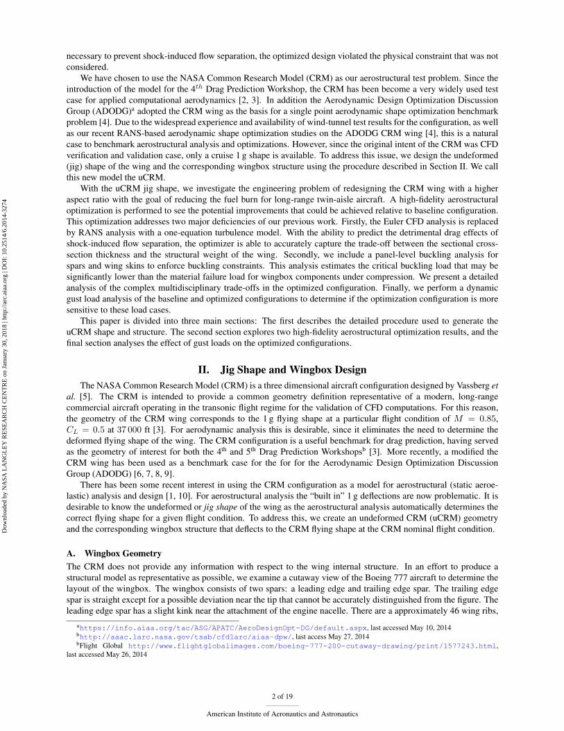
A. Wingbox Geometry The CRM does not provide any information with respect to the wing internal structure. In an effort to produce a structural model as representative as possible, we examine a cutaway view of the Boeing 777 aircraft to determine the layout of the wingbox. The wingbox consists of two spars: a leading edge and trailing edge spar. The trailing edge spar is straight except for a possible deviation near the tip that cannot be accurately distinguished from the figure. The leading edge spar has a slight kink near the attachment of the engine nacelle. There are a approximately 46 wing ribs,
ahttps://info.aiaa.org/tac/ASG/APATC/AeroDesignOpt-DG/default.aspx, last accessed May 10, 2014 bhttp://aaac.larc.nasa.gov/tsab/cfdlarc/aiaa-dpw/, last access May 27, 2014 bFlight Global http://www.flightglobalimages.com/boeing-777-200-cutaway-drawing/print/1577243.html,
last accessed May 26, 2014
2 of 19
American Institute of Aeronautics and Astronautics

Dow
nloa
ded
by N
ASA
LA
NG
LE
Y R
ESE
AR
CH
CE
NT
RE
on
Janu
ary
30, 2
018
| http
://ar
c.ai
aa.o
rg |
DO
I: 1
0.25
14/6
.201
4-32
74
not including the close-out rib structure used for the wingbox-body attachment. Most ribs are perpendicular to the trailing edge spar and this results in several ribs near the root intersecting the root rib close-out structure.
Figure 1: Boeing 777 (Left) and CRM (right). The CRM has a slightly smaller area wing and 3.5°more wing sweep than the Boeing 777.
The left side of Figure 1 shows the planform view of the 777-200ER extracted from the aircraft planning document [11] with a best-guess superimposed wingbox geometry based on the cutaway drawing. We have chosen to ignore the small break in the leading edge spar for the sake of simplicity. This estimate of the geometry of the Boeing 777 wingbox could not be used directly in the CRM wing due to 3.5°more sweep on the CRM. Instead, a wingbox with the same proportions (front and rear spar location, rib spacing, etc.) and structural layout as the Boeing 777 are used. Using digital versions of the Boeing 777 drawing, the extents of the wingbox are measured as a fraction of local chord local chord (Table 1). These percentages are rounded and are then used to define the outline of the CRM wingbox. The rib spacing for the CRM wingbox is chosen to be approximately the same as for the Boeing 777, with a normal-distance spacing of 73.15 cm (28.8 in). Since the CRM wing has a slightly lower span than the Boeing 777, there are 49 ribs in total total including 4 ribs on the center wingbox section.
777 Estimated (%) uCRM Wingbox (%)
Leading edge spar root 10.4 10 Leading edge spar tip 36.1 35 Trailing edge spar root 59.6 60 Trailing edge spar tip 60.7 60
Table 1: Locations (in % local chord) estimated for the Boeing 777 and values used for the uCRM wingbox
Having determined the planform of the wingbox, we used an in-house tool to generate the geometry of the wingbox and the internal components [12]. This initial wingbox geometry conforms to the original CRM outer mold line. The geometry of the wingbox structure is shown in Figure 2. The meshing of the wingbox is performed using ICEMCFD.
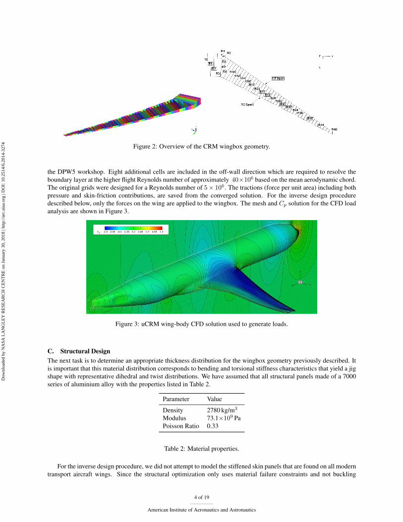
B. Loads A set of representative aerodynamic loads is required to find the undeformed shape of the wing. These aerodynamic loads are generated using the CRM wing-body configuration at the following nominal flight condition: M = 0.85, CL = 0.5 altitude = 37 000 ft. The mesh used is a modified version of the multi-block ‘’Tiny” mesh provided for
3 of 19
American Institute of Aeronautics and Astronautics
Dow
nloa
ded
by N
ASA
LA
NG
LE
Y R
ESE
AR
CH
CE
NT
RE
on
Janu
ary
30, 2
018
| http
://ar
c.ai
aa.o
rg |
DO
I: 1
0.25
14/6
.201
4-32
74
Figure 2: Overview of the CRM wingbox geometry.
the DPW5 workshop. Eight additional cells are included in the off-wall direction which are required to resolve the boundary layer at the higher flight Reynolds number of approximately 40×106 based on the mean aerodynamic chord. The original grids were designed for a Reynolds number of 5 × 10⁶. The tractions (force per unit area) including both pressure and skin-friction contributions, are saved from the converged solution. For the inverse design procedure described below, only the forces on the wing are applied to the wingbox. The mesh and Cp solution for the CFD load analysis are shown in Figure 3.
Figure 3: uCRM wing-body CFD solution used to generate loads.
C. Structural Design The next task is to determine an appropriate thickness distribution for the wingbox geometry previously described. It is important that this material distribution corresponds to bending and torsional stiffness characteristics that yield a jig shape with representative dihedral and twist distributions. We have assumed that all structural panels made of a 7000 series of aluminium alloy with the properties listed in Table 2.
Parameter Value
Density 2780 kg/m3
Modulus 73.1×10⁹ Pa Poisson Ratio 0.33
Table 2: Material properties.
For the inverse design procedure, we did not attempt to model the stiffened skin panels that are found on all modern transport aircraft wings. Since the structural optimization only uses material failure constraints and not buckling
4 of 19
American Institute of Aeronautics and Astronautics

Dow
nloa
ded
by N
ASA
LA
NG
LE
Y R
ESE
AR
CH
CE
NT
RE
on
Janu
ary
30, 2
018
| http
://ar
c.ai
aa.o
rg |
DO
I: 1
0.25
14/6
.201
4-32
74
constraints, this simplified model is sufficient to yield a reasonable bending and torsion stiffness distribution. In reality, the skins would be thinner with the extra material added as stiffeners to substantially increase buckling resistance. We determined the material distribution of the wingbox with structural optimization. This optimization used a single 2.5 g load including inertial and fuel load relief. The results of the structural optimization are given in Table 3. The labeled structural layout is given in Figure 2. We assume that the upper and lower surface wing panels have the same thickness and the resulting mass of this simple wingbox structure is 12 263 kg.
Component Skin patch boundaries Thickness (mm)
Skin LE spar, Te Spar, R0, R2 14.0 Skin LE spar, Te Spar, R2, R4 19.0 Skin LE spar, R4, R8, 21.0 Skin LE spar, TE spar, R8, R11 22.0 Skin LE spar, TE spar, R11, R13 19.0 Skin LE spar, TE spar, R13, R15 20.0 Skin LE spar, TE spar, R15, R17 21.0 Skin LE spar, TE spar, R17, R19 26.0 Skin LE spar, TE spar, R19, R21 24.0 Skin LE spar, TE spar, R21, R23 21.0 Skin LE spar, TE spar, R23, R25 21.0 Skin LE spar, TE spar, R25, R27 20.0 Skin LE spar, TE spar, R27, R29 18.0 Skin LE spar, TE spar, R29, R31 17.0 Skin LE spar, TE spar, R31, R33 14.0 Skin LE spar, TE spar, R34, R37 11.0 Skin LE spar, TE spar, R37, R40 8.2 Skin LE spar, TE spar, R40, R43 5.2 Skin LE spar, TE spar, R43, R46 2.4 Skin LE spar, TE spar, R46, R47 2.0
Ribs All 2.0 LE Spar All 5.0 TE Spar All 5.0
Table 3: Thickness distribution on structural model.
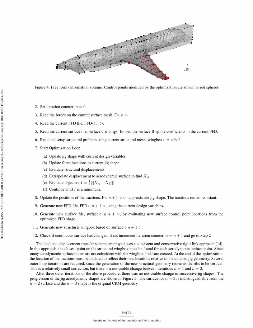
D. Geometric Manipulation The inverse design procedure requires a method capable of applying smooth perturbations to existing geometries. The free-form deformation (FFD) approach is ideal for this task [13]. The FFD volume used to manipulate the geometry is shown in Figure 4. Cubic B-spline basis functions in the span-wise and chord-wise directions ensure that the final jig geometry will be smooth. The design variables are the displacements of each of the 98 control points in the x, y and z directions.
III. Inverse Design Procedure In this section we describe the inverse-design procedure used to generate the uCRM jig shape. We have chosen
to treat the inverse-design procedure as a geometric least-squares minimization problem. We use a geometric manipulation tool to determine the geometry of both the internal structure and the undeformed aerodynamic surface. After applying the fixed loads to the jig structural model, we check how close the deformed aerodynamic surface matches the
1CRM wing-only geometry surface. The objective function, I = l|XA −XT l| is the L2 norm of these differences. 2 The design variables for the unconstrained minimization are the x, y, and z coordinate displacements of 98 control points leading to 294 design variables.
The procedure for finding the uCRM jig shape is as follows:
1. Read coordinates of the CRM, XT . These are known as the target coordinates.
5 of 19
American Institute of Aeronautics and Astronautics
Dow
nloa
ded
by N
ASA
LA
NG
LE
Y R
ESE
AR
CH
CE
NT
RE
on
Janu
ary
30, 2
018
| http
://ar
c.ai
aa.o
rg |
DO
I: 1
0.25
14/6
.201
4-32
74 Figure 4: Free form deformation volume. Control points modified by the optimization are shown as red spheres
.
2. Set iteration counter, n = 0
3. Read the forces on the current surface mesh, F< n >.
4. Read the current FFD file, FFD< n >.
5. Read the current surface file, surface< n >.igs. Embed the surface B-spline coefficients in the current FFD.
6. Read and setup structural problem using current structural mesh, wingbox< n >.bdf
7. Start Optimization Loop:
(a) Update jig shape with current design variables
(b) Update force locations to current jig shape
(c) Evaluate structural displacements
(d) Extrapolate displacement to aerodynamic surface to find XA
1(e) Evaluate objective I = l|XA − XT l|2
(f) Continue until I is a minimum.
8. Update the positions of the tractions, F< n + 1 > on approximate jig shape. The tractions remain constant.
9. Generate new FFD file, FFD< n + 1 >, using the current design variables.
10. Generate new surface file, surface< n + 1 >, by evaluating new surface control point locations from the optimized FFD shape.
11. Generate new structural wingbox based on surface< n + 1 >.
12. Check if continuous surface has changed, if so, increment iteration counter, n = n + 1 and go to Step 2
The load and displacement transfer scheme employed uses a consistent and conservative rigid-link approach [14]. In this approach, the closest point on the structural wingbox must be found for each aerodynamic surface point. Since many aerodynamic surface points are not coincident with the wingbox, links are created. At the end of the optimization, the location of the tractions must be updated to reflect their new locations relative to the updated jig geometry. Several outer loop iterations are required, since the generation of the new structural geometry reorients the ribs to be vertical. This is a relatively small correction, but there is a noticeable change between iterations n = 1 and n = 2.
After three outer iterations of the above procedure, there was no noticeable change in successive jig shapes. The progression of the jig aerodynamic shapes are shown in Figure 5. The surface for n = 3 is indistinguishable from the n = 2 surface and the n = 0 shape is the original CRM geometry.
6 of 19
American Institute of Aeronautics and Astronautics

Dow
nloa
ded
by N
ASA
LA
NG
LE
Y R
ESE
AR
CH
CE
NT
RE
on
Janu
ary
30, 2
018
| http
://ar
c.ai
aa.o
rg |
DO
I: 1
0.25
14/6
.201
4-32
74
Figure 5: Progression of the jig aerodynamic surface.
A. Verification of the Jig Shape To validate the uCRM design, we compare the Cp distribution of the CRM wing-body configuration with an aerostructural analysis performed on the uCRM (Figure 6). This final verification is necessary, as the inverse design procedure only guarantees that the computed jig shape is as close as possible to the target geometry, given the degrees of freedom available to the optimization. The two sets of contours match closely, although there are slight differences, even at the
Figure 6: Cp contours comparison of CRM wing-body and uCRM aerostructural solution.
root. The slight differences at the root can be attributed to the slight angle of attack difference in the aerostructural solution that has been adjusted to match the same lift coefficient as the CRM wing-body configuration. The largest variation between the two solutions occurs near the wingtip, where the geometries have the largest discrepancy. The aerostrucutural uCRM solution appears to be have a slightly stronger shock over the outer 10% of the semi-span which may be responsible for the higher drag coefficient seen in Table 4. Even so, the drag coefficient values differ by less than one drag count, which we consider acceptable. The largest geometric difference between the two configurations is approximately 8 cm at trailing edge of the wingtip, which corresponds to only about 1% of the mean aerodynamic chord.
As we can see in Figure 5, the uCRM has almost zero dihedral over the outer sections of the wing. This indicates that almost all of the span-wise wing curvature in the CRM geometry is due to aerostructural effects. We have also extracted the wing-twist distribution of the uCRM configuration and compared it to the original geometry (Figure 7). The difference in twist near the wingtip is approximately 4°and this gap reduces to zero near the root. The uCRM has a nearly constant twist over outer half of semi-span. This twist difference highlights how important aeroelastic effects on swept transonic wings can be, even at a cruise condition. This jig-twist twist distribution is comparable to the twist distribution found using a similar procedure carried out by Klimmek [10] who used a panel code for the aerodynamic model.
7 of 19
American Institute of Aeronautics and Astronautics

Dow
nloa
ded
by N
ASA
LA
NG
LE
Y R
ESE
AR
CH
CE
NT
RE
on
Janu
ary
30, 2
018
| http
://ar
c.ai
aa.o
rg |
DO
I: 1
0.25
14/6
.201
4-32
74
Parameter CRM wing-body uCRM Aerostructural
CL 0.5 0.5 CD (ct) 231.37 232.26 α 1.857 1.823
Table 4: Aerodynamic coefficient comparison
2y/b
Twist
0 0.2 0.4 0.6 0.8 16
4
2
0
2
4
6
CRM
uCRM
Figure 7: Comparison of twist between CRM and the uCRM (jig shape).
Since the exact aerostructural solution, (including the tip displacement) depends on the flight condition and the specifics of the structural solver, aerodynamic solver, and load and displacement transfer schemes, there are many possible sources for discrepancies. Given all these possible sources of error, we feel that this uCRM geometry is a representative jig shape for the CRM configuration. The final shape modifications have been applied to the original CRM surface definition and will be made publicly available. We hope that the widespread availability of the uCRM geometry will encourage more researchers to consider the Common Research Model for aerostructural and aeroelastic design studies.
IV. High Fidelity Aerostructural Optimization In this section we present a sample high fidelity aerostructural optimization using the uCRM configuration as the
initial design. The optimization problem can be best described as a complete wing redesign for the CRM. Based on previous work by the authors [15, 1] we know that a fuel burn minimization problem places more emphasis on reducing drag, at the expense of increased structural weight, and tends to produce very flexible wing designs. We make an effort to simplify the optimization problem as much as possible, both in an effort to reduce the computational expense, and also to more fully understand the trade-offs in the optimization. We are primarily interested in the overall planform, the t/c distribution, and the aspect ratio of the optimized design.
The presented optimization is representative of a wing-redesign project that is fairly common in transport aircraft design. Many stretched variants of commercial aircraft use a re-designed wing, while maintaining backwards compatibility with the remainder of the existing design.
A. Methodology This section provides a brief overview of the techniques we use for the optimization. The overall framework is called MACH— multidisciplinary design optimization (MDO) of aircraft configurations with high fidelity [16]. With this set of tools, it is possible to perform high fidelity aerostructural analysis and optimization of full aircraft configurations. Design variables may include any type of geometric perturbation, parametrizations of the structural model, as well as
8 of 19
American Institute of Aeronautics and Astronautics
Dow
nloa
ded
by N
ASA
LA
NG
LE
Y R
ESE
AR
CH
CE
NT
RE
on
Janu
ary
30, 2
018
| http
://ar
c.ai
aa.o
rg |
DO
I: 1
0.25
14/6
.201
4-32
74
purely aerodynamic variables such as angle of attack, Mach number or altitude. For completeness, a short summary of the main components of the framework is presented below.
1. Geometric Parametrization
Geometric parametrizations of both the aerodynamic and structural disciplines use the free-form deformation (FFD) approach [13]. This approach is especially well suited to aerostructural optimization, since it provides uniform treatment of both the wetted CFD surface and the structural mesh. A grouping approach of the FFD control points enables the use of planform level variables that control the overall shape of the wing. The overall shape variables include span, sweep, chord, twist and, local variables defining cross-sectional airfoil shapes. The FFD used in the optimization is similar to the one in Figure 4 with the exception that there are 12 equally spaced chord-wise control points on the upper and lower surfaces.
2. CFD Solver and Mesh Deformation
To accurately predict the total drag on an aircraft operating in the transonic flow regime, we solve use a Reynolds-Averaged Navier Stokes (RANS) model. The CFD solver, SUmb [17], solves the RANS equations using a finite-volume, cell-centred multiblock technique. The mean flow equations solved using semi-implicit alternating direction implicit (ADI) scheme, which is accelerated using geometric multigrid. The 1-equation Spalart–Allmaras turbulence model is loosely coupled to the mean flow equations and is iterated using a diagonally dominant alternating direction implicit (DDADI) method. A discrete adjoint method for the Euler and RANS equations is implemented within SUmb [18, 19], enabling the efficient computation of gradients of functions of interest with respect to any number of design variables. More information of the RANS adjoint implementation is given Lyu [18].
MACH uses the hybrid algebraic-linear elastic approach described in Kenway et al. [20]. However, the relatively simple mesh topology of the DPW5 meshes allows us to use the algebraic scheme alone, which is a delta-based transfinite interpolation method [21].
3. Structural Solver
The MACH structural solver is the toolkit for the analysis of composite structures (TACS) by Kennedy and Martins [22]. For the thin-shell problems typical of transport aircraft wingboxes, it is possible to have matrix condition p numbers that exceed O 109 . For this reason, we use a parallel direct method to solve the structural governing equations.
4. Aerostructural Solver
The aerostructural solver is responsible for two main tasks: Solving the nonlinear aerostructural system of equations, and solving the linear adjoint equations. Nonlinear block Gauss–Seidel (NLBGS) with Aitken acceleration [23] is used for the non-linear system which has proven sufficiently robust for the range of flight conditions considered. The adjoint system uses the coupled Krylov (CK) method [16], which has a significant speed advantage over the traditional linear block Gauss–Seidel (LBGS) solver.
5. Optimization Algorithm
The high computational cost of aerostructural solutions, and the large number of optimization design variables necessitates the use of an efficient gradient-based optimization algorithm. The optimization algorithm for all results in the paper (including the inverse design problem in the previous section) is SNOPT (sparse nonlinear optimizer) [24]. SNOPT is coupled to the MACH framework through the Python interface pyOpt [25].
B. Optimization Problem Description In this section we provide a complete description of the optimization problem. The objective is to reduce the fuel consumption for the nominal long-range design mission. For simplicity we ignore the fuel burn associated with the taxi, take-off climb and descent phases. Instead, we use the Breguet range equation applied to the full design range:
R TSFCFB = LGW exp − 1 , (1)
V (L/D)
9 of 19
American Institute of Aeronautics and Astronautics
Dow
nloa
ded
by N
ASA
LA
NG
LE
Y R
ESE
AR
CH
CE
NT
RE
on
Janu
ary
30, 2
018
| http
://ar
c.ai
aa.o
rg |
DO
I: 1
0.25
14/6
.201
4-32
74
where FB is the fuel burn, LGW is the aircraft landing weight, R is the design mission range, TSFC is the thrust-specific fuel consumption, V is the cruise speed, and L/D is the lift-to-drag ratio. Since we only model the wing-body, 50 counts of drag are added to the CFD computed drag coefficient to account for the horizontal stabilizer, vertical stabilizer, nacelles and pylons. The landing weight is computed using the following formula:
LGW = 1.25 × W + Fixed Weight + Reserve Fuel Weight + Secondary Wing Weight (2)
where W is the weight computed by the structural FE model. The factor of 1.25 accounts for additional weight associated with fasteners, overlaps, and other components not modeled in the idealized wingbox. As discussed in Section II, the overall size of the CRM configuration is similar to a Boeing 777-200ER. Additional information required to define the aerostructural optimization problem is obtained using publicly available data [11] (see Table 5).
Table 5: CRM specifications
Parameter Value Units
Cruise Mach number 0.85 Cruise lift coefficient 0.5 Initial cruise altitude 37 000 ft Span 58.8 m Aspect ratio 9.0 Reference wing area 383.7 m2
Sweep (leading edge) 37.4 ◦
Maximum take-off weight (MTOW) 297 500 kg Maximum landing weight (MLW) 213 180 kg Maximum zero fuel weight (MZFW) 195 040 kg Operational empty weight 138 100 kg Design range 7 725 nm Design payload 34 000 kg Reserve fuel 15 000 kg Initial wing weight 30 286 kg Fixed weight 107 814 kg Thrust specific fuel consumption (cT ) 0.53 lb/(lbf · h)
The optimization requires the analysis of three different operating conditions. A cruise flight condition at the design Mach number of 0.85 provides the L/D ratio for the Breguet range equation to compute the total fuel burn. Two additional maneuver conditions are required for the evaluation of the structural constraint functions. Maneuver case 1 is a 2.5 g symmetric pull-up maneuver at M = 0.85 and 10 000 ft altitude. Maneuver case 2 is a −1.0 g symmetric push-over maneuver at M = 0.60 at sea level.
The initial wing weight is estimated from a structural optimization preformed before the start of the aerostructural optimization. The structural model for the high fidelity optimizations differs from the model used for the inverse design procedure in three ways:
1. The center wingbox is removed, leaving only the main wingbox. When the full structural model is used, there exists a small, but non-zero structural displacement at the wing-body fuselage junction. Since fuselage portion of the CFD geometry is fixed (and thus does not provide loads to the wingbox) a discrepancy arises where wing-body junction displaces, but the fuselage nodes surrounding it do not. If the wing-body junction displacements become large, a surface tear will appear, leading to invalid mesh and failure of the optimization process.
2. The second-order elements are converted to third-order elements resulting in 190 710 total degrees of freedom.
3. A more sophisticated panel-level analysis is used. The simple unstiffened panels used for the uCRM design are not suitable for more detailed analysis due to the low panel buckling resistance. To remedy this, we use a smeared-stiffness panel approach. The cross section of the wing skins and spars are assumed to have the general cross section shown in Figure 8. For simplicity we assume that tw = tb and wb = hs. This panel model can then be used to perform a panel-level buckling analysis of the stiffened panel. Several independent buckling modes are computed, including buckling of the skin between stiffeners, buckling of the stiffeners, and overall panel buckling including stiffeners and skins. The critical case is determined by aggregating the buckling modes using a Kreisselmeier–Steinhauser (KS) function [26, 27]. Further details of this approach can be found in previous work by the authors [15].
10 of 19
American Institute of Aeronautics and Astronautics

Dow
nloa
ded
by N
ASA
LA
NG
LE
Y R
ESE
AR
CH
CE
NT
RE
on
Janu
ary
30, 2
018
| http
://ar
c.ai
aa.o
rg |
DO
I: 1
0.25
14/6
.201
4-32
74
b
wb
hs
tstb
tw
Figure 8: The panel geometry and thickness design variables used in the structural design parametrization.
To fully exploit the benefits of high-fidelity aerostructural optimization a large number of design variables are used. There are three groups of design variables: Geometric design variables, aerodynamic variables and structural variables. The geometric design variables include the wing span, sweep, chord, twist distribution and detailed shape control over the airfoil cross sections. The span, sweep and chord variables yield a tremendous amount of design freedom typically not found in high fidelity aerodynamic only optimization. In particular, the optimization process is free to explore the trade-off between increasing the wingspan to reduce the span-loading and thus induced drag at the expense of a potentially heavier structure. Likewise, the sweep angle may be modified in response to changes in the airfoil thickness distributions as well as accounting for the change in structural mass. The four aerodynamic variables include the angle of attack the cruise and each of the maneuver flight conditions and the altitude for the cruise condition. The remainder of the design variables are used for the parametrization of the structural wingbox. The first 4 variables are the stiffener pitch of the upper skin, lower skin, leading edge spar and trailing edge spar. We assume that the stiffener pitch is thus constant across each component. The panel-based smeared stiffness approach results in 3 design variables the skin or spar in each rib bay: Panel thickness, stiffener thickness, stiffener height. An additional variable, the panel length, is used to simplify panel buckling computations and is constrained to match the physical panel length (which changes as a function of the geometric design variables) through an equal number of nonlinear constraints. Altogether, there are 944 design optimization variables.
Even with high fidelity analyses, the optimization problem requires many constraints. The first three constraints are to insure steady flight, which required that the lift equals the weight multiplied by the load factor, n. The weight for the cruise condition is computed from:
Wcruise = LGW + 0.20 × FB. (3)
This weight is approximately equal to the lift generated by the CRM at the nominal cruise condition of M = 0.85, CL = 0.5 at 37 000 ft. The analysis weight for each of the two maneuver conditions is taken to be takeoff gross weight, TOGW = LGW + FB. We use a constraint on the actual lift coefficient in addition to the previously described lift constraint. Due to the change in dynamic pressure as the altitude changes, the coefficient of lift will change for a fixed lift. This constraint is used to ensure that the optimized design, at the optimization determined optimum altitude, has a least a 1.3 g margin to initial buffet. The constraint value of 0.525 assumes an initial buffet onset at at a CL of 0.6825. A variety of geometric constraints are used to ensure a a realistic design is produced. The leading edge radius constraint ensure no reduction in leading edge radius, potentially causing reduction in the low-speed
performance. Previous aerodynamic optimizations have shown that single point optimized designs without CLmax
this constraint produce very sharp leading edges in transonic flow [28]. The trailing edge constraints are used to ensure a manufacturable trailing edge that is not too thin. The trailing edge spar-height constraint ensure a sufficient vertical height is available for the necessary actuation mechanisms for the flap and ailerons. The exposed wing area is fixed to initial area which avoids accounting for the changes in the secondary weight as the wing area changes. The volume constraint ensures that the same wing volume is available for fuel as in the initial design. The 2.5 g maneuver condition uses 3 KS stress constraints aggregation functions: One for the upper wing surface, a second for the lower wing surface and a final one for the ribs and spars. Two buckling constraints are used for the upper skin and ribs/spars. For the −1.0 g condition, only the rib/spar stress constraint is used along with lower surface and rib/spar buckling. We use several hundred adjacency constraints that ensure there are no large changes in the properties of skin or stiffener between adjacent panels. Finally, there are 16 constraints for the FFD airfoil shape variables that leading and trailing edges from moving. This is required to eliminate a “shearing twist” design mode and allows the pure rotation (nonlinear) twist to modify the overall wing twist. The structural adjacency constraints and leading edge/trailing edge constraints are linear and are always satisfied exactly at each optimization iteration by SNOPT [24]. In total, there are 938 optimization constraints.
11 of 19
American Institute of Aeronautics and Astronautics

Dow
nloa
ded
by N
ASA
LA
NG
LE
Y R
ESE
AR
CH
CE
NT
RE
on
Janu
ary
30, 2
018
| http
://ar
c.ai
aa.o
rg |
DO
I: 1
0.25
14/6
.201
4-32
74
Function/variable Description Quantity minimize Fuel burn
with respect to xspan Wing span 1 xsweep Wing sweep 1 xchord Wing chord 1 xtwist Wing twist 8 xairfoil FFD control points 192 xalphai
Angle of attack at each flight condition 3 xaltitude Cruise altitude 1 xskin pitch Upper/lower stiffener pitch 2 xspar pitch Le/Te Spar stiffener pitch 2 xribs Rib thickness 45 xpanel thick Panel thickness Skins/Spars 172 xstiff thick Panel stiffener thickness Skins/Spars 172 xstiff height Panel stiffener height Skins/Spars 172 xpanel length Panel length Skin/Spars 172
Total design variables 944
subject to L = niW Lift constraint 3 CL < 0.525 1.3 g cruise buffet boundary 1 tLE/tLEInit ≥ 1.0 Leading edge radius 20
≥ 1.0 Trailing edge thickness 20tTE/tTEInit
(t/c)TE Spar ≥ 0.80(t/c)TE sparinit Minimum trailing edge spar height 20
A - Ainit = 0.0 Fixed exposed wing area 1
V /Vinit ≥ 1.0 Minimum fuel volume 1
Lpanel − xpanel length = 0 Target panel length 172 KSstress ≤ 1 2.5 g Yield stress 3 KSbuckling ≤ 1 2.5 g Buckling 2 KSstress ≤ 1 -1.0 g Yield stress 1 KSbuckling ≤ 1
xpanel thicki − xpanel thicki+1
≤ 0.0025
≤ 0.0025
-1.0 g Buckling
Skin thickness adjacency Stiffener thickness adjacency − xstiff thicki+1xstiff thicki xstiff heighti
− xstiff heighti+1
Stiffener height adjacency xstiff thick − xpanel thick < 0.005 Maximum stiffener-skin difference 172 ΔzTE,upper = −ΔzTE,lower Fixed trailing edge 8 ΔzLE,upper = −ΔzLE,lower Fixed leading edge 8
Total constraints 938
C. Optimization results The optimization is performed using 60 processors with 52 dedicated to the CFD analysis and 8 dedicated to the structural analysis. Each of the three analysis conditions are executed in sequence. Approximately 150 majors iterations are completed in 30 hours. At the optimum, all constraints are satisfied. A summary of the key parameters during the optimization is shown in Figure 9.
Feasibility refers to the maximum constraint violation, and it is a measure of how closely the nonlinear constraints are satisfied. Optimality refers to how closely the current point satisfies the first-order Karush–Kuhn–Tucker (KKT) conditions [29]. Approximately 2 orders of magnitude reduction in the optimality are achieved, which is similar to previous aerostructural [1] and aerodynamic optimizations [28]. A complete overview of optimized configuration with the initial design is shown in Figure 10.
12 of 19
American Institute of Aeronautics and Astronautics
2
168
168
168

Dow
nloa
ded
by N
ASA
LA
NG
LE
Y R
ESE
AR
CH
CE
NT
RE
on
Janu
ary
30, 2
018
| http
://ar
c.ai
aa.o
rg |
DO
I: 1
0.25
14/6
.201
4-32
74
Iteration
Win
g m
as
s (
kg
)
Sp
an
L/D
0 50 100 150
26000
28000
30000
32000
34000
56
58
60
62
64
66
68
70
17
17.5
18
18.5
19
19.5
20
Fu
el b
urn
(k
g)
Fe
as
ibilit
y
Op
tim
ality
100000
105000
110000
115000
106
105
104
103
102
104
103
102
101
Figure 9: Evolution of key variables during optimization.
13 of 19
American Institute of Aeronautics and Astronautics

Dow
nloa
ded
by N
ASA
LA
NG
LE
Y R
ESE
AR
CH
CE
NT
RE
on
Janu
ary
30, 2
018
| http
://ar
c.ai
aa.o
rg |
DO
I: 1
0.25
14/6
.201
4-32
74
Initial Span=58.8 m Aspect ratio:9.0 Wing mass:30286 kg TOGW:299375 kg Fuelburn=112276kg
c,: -1.0 -0.5 0.0 0.5 1.0
Normalized Lift 2
-------------. 1.5_-
Elliptical j< :o.5
0
Twist 5
-1.0g 0
1.0g -5 -- 2.5g --
-10
tic 0.2
0.15
0.1
0.05
Optimized Span:68.9 m Aspect ratio=12.6 Wing mass:30983 kg TOGW:290142 kg Fuel burn=102345 kg
D
X
-1 -
-0.5
0 ~
0
0.5
-1 -
-0.5
0 ~
0
0.5
z t,,( mm): 4 6 8 1012141618202224
~y
X
Buckling: 0.00 0.26 0.53 0.79 Stress: 0.10 0.38 0.66 0.94
-0.5
0 ~
0
0.5
-1 -
-0.5
0 ~
0
0.5
14 of 19
Am
erican Institute of Aeronautics and A
stronautics
Figure 10: Aerostructural optimization result: Cp and planform comparison with initial design (upper left); equivalent thickness distribution, stress and buckling KS failure criteria (upper right); comparison of initial and optimized lift distributions, twist distributions and thickness to chord ratio (t/c) (lower left); four airfoils with corresponding Cp distributions (lower right).

Dow
nloa
ded
by N
ASA
LA
NG
LE
Y R
ESE
AR
CH
CE
NT
RE
on
Janu
ary
30, 2
018
| http
://ar
c.ai
aa.o
rg |
DO
I: 1
0.25
14/6
.201
4-32
74
The objective—fuel burn—is reduced from the initial value of 112 276 kg to 102 345 kg, a reduction of 8.8%. The TOGW for the design mission of 7 725 nm is reduced by almost the same amount, except for the small increase in wing mass of 697 kg. The increase in lift to drag ratio from the initial value of 17.84 to the optimized value of 19.28 can be attributed to several factors: 1. The cruise angle of attack is increased up to the limit of 2.5°, yielding slightly more fuselage lift and lower induced drag due to the fuselage. 2. The elimination of the upper surface wing shock through airfoil shape modifications and an increase in sweep. 3. An increase in cruise altitude to 38 700 ft. 4. An increase in the wingspan from 58.8 m to 68.9 m.
Table 6 presents a breakdown of the drag into pressure and skin-friction components. Note that the constant drag C2
Lmark-up of 50 counts is not included in this table. The ideal induced drag is computed from CDi = πAR , assuming an Oswald efficiency factor of 1.0. From the increase in aspect ratio alone, we would expect a drag decrease of 28.2 counts. The pressure drag includes the induced drag, wave drag and viscous pressure drag. The wave drag decreased, as evidenced by the elimination of the shock and the parallel isobars on the Cp distribution. However, the optimized lift distribution does not match the elliptical distribution as closely as the baseline configuration, incurring an induced drag penalty.
The thickness to chord ratio is increased substantially over the majority of the span from which we expect slightly increased viscous pressure drag. Finally, the decrease in the wing chord and increase in altitude, both of which lower the Reynolds number, caused an increase in the skin-friction drag by 2.5 counts. Taking all these effects together, there is a 22.4 count reduction in drag—20% lower than would be expected from linear aerodynamic assumptions. All of these complex aerodynamic iterations are physically modeled and can only be accurately predicted using high-fidelity CFD analysis.
CL Ideal CDiCDtotal CDp CDv
Initial 0.525 244.7 154.8 89.9 97.5 Optimized 0.525 222.3 129.8 92.5 69.3
Difference 0.000 22.4 25.0 −2.6 28.2
Table 6: Drag breakdown for baseline and optimization configuration
Remarkably, the 10.1 m span increase, and associated 40% increase in aspect ratio from 9.0 to 12.6, is achieved with almost zero weight penalty. To understand how such a result is possible, we need to examine the spanwise lift distributions of the initial and optimized designs. The normalized lift plot in Figure 9 shows how the 2.5 g maneuver lift distribution is shifted inboard, and there is slightly negative lift near the tip. This is highly desirable from a structural perspective and the optimizer has successfully exploited a large amount of aeroelastic tailoring to reduce the load for the maneuver load cases. The twist distribution reveals the increased torsional flexibility of the optimized design, resulting more washout for the 2.5 g load condition and more wash-in for the −1.0 g condition.
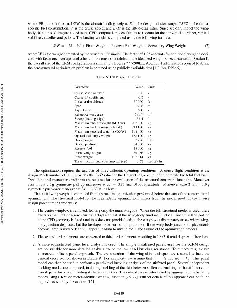
The thickness-to-chord ratio has increased for the optimized design relative to the initial. However, this is offset by the reduction in chord, which results in little change in the maximum physical height of the optimized spar box relative to the initial design (Figure 11). The front view of the initial and optimized configuration showing the jig shape, −1.0 g, 1.0 g, and 2.5 g shape provides further insight into the how the optimized design is able to use passive aeroelastic tailoring. For the initial design the tip displacement gap between the 1.0 g and 2.5 g conditions is slightly larger than the displacement gap between the jig and 1.0 g conditions. However, for the optimized configuration, the 2.5 g deflection is much lower than would be expected given the deflection at the cruise configuration. This is due primarily to the inboard load shifting caused by the optimal aeroelastic tailoring.
The upper structural figure shows the equivalent skin thickness distribution, defined to be to skin thickness with the same mass (but not stiffness properties) as the skin stiffened panel. It provides an overview of the overall material distribution of the spar box primary structure. Since the wing mass increased by only 2.3% and the projected area of the sparbox is fixed, the overall teq is similar. The only significant change is a slight decrease in teq near the Yehudi break and an a corresponding increase near the wing root. The upper wing-surface and spars show the buckling criteria for the 2.5 g maneuver condition while the lower surface shows the stress failure criteria for the same flight condition. All stress and buckling constraint values are lower than the upper limit of 1.0. However, as we will explored in the next section, other load cases that have not been considered in the optimization may have a significant effect on the design.
15 of 19
American Institute of Aeronautics and Astronautics
Dow
nloa
ded
by N
ASA
LA
NG
LE
Y R
ESE
AR
CH
CE
NT
RE
on
Janu
ary
30, 2
018
| http
://ar
c.ai
aa.o
rg |
DO
I: 1
0.25
14/6
.201
4-32
74
2y/bt
(m)
0 0.2 0.4 0.6 0.8 10
0.5
1
1.5
2
Initial
Optimized
Figure 11: Maximum spar-box depth
V. Unsteady Gust Analysis The key factor driving the wing design for the fuel-burn minimization described in the previous section is the
increase in aspect ratio, which reduces the induced drag. The increased wing flexibility gives the optimizer a significant amount of freedom to tailor favorable maneuver lift distributions thus allowing the aspect ratio increase without a significant mass penalty. However, we did not impose any failure or buckling constraints at the cruise condition or other potentially critical load cases with load distributions that are close to cruise distribution.
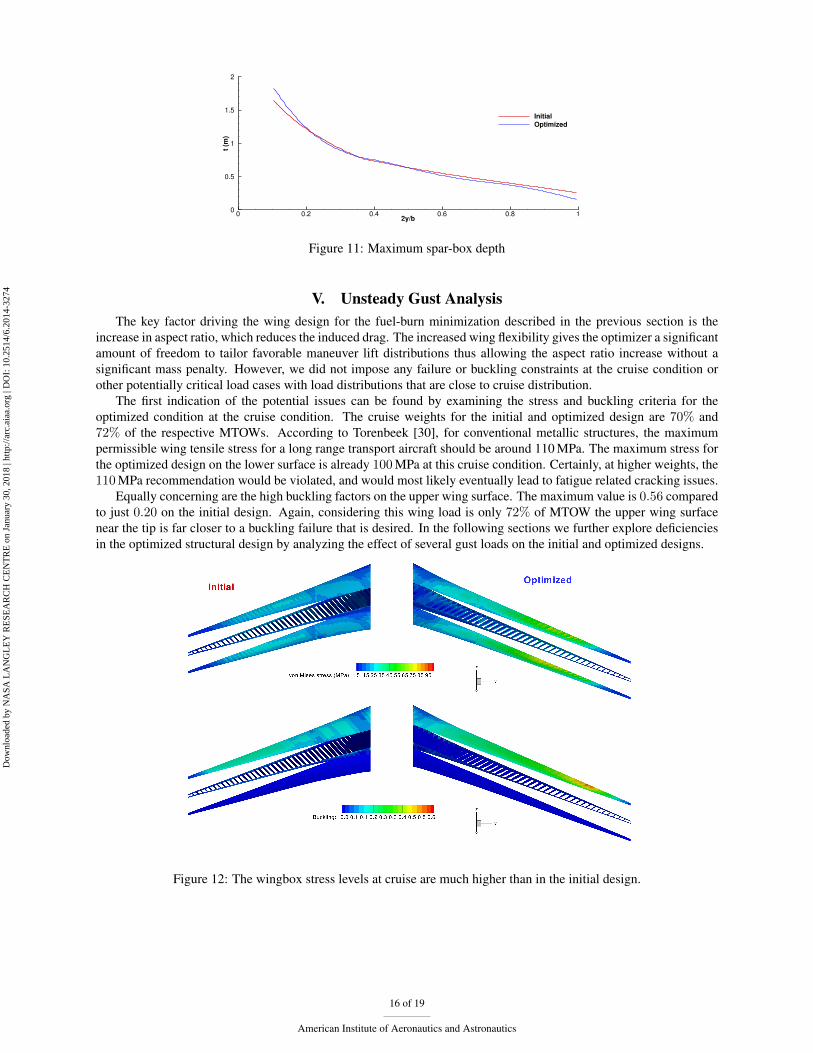
The first indication of the potential issues can be found by examining the stress and buckling criteria for the optimized condition at the cruise condition. The cruise weights for the initial and optimized design are 70% and 72% of the respective MTOWs. According to Torenbeek [30], for conventional metallic structures, the maximum permissible wing tensile stress for a long range transport aircraft should be around 110 MPa. The maximum stress for the optimized design on the lower surface is already 100 MPa at this cruise condition. Certainly, at higher weights, the 110 MPa recommendation would be violated, and would most likely eventually lead to fatigue related cracking issues.
Equally concerning are the high buckling factors on the upper wing surface. The maximum value is 0.56 compared to just 0.20 on the initial design. Again, considering this wing load is only 72% of MTOW the upper wing surface near the tip is far closer to a buckling failure that is desired. In the following sections we further explore deficiencies in the optimized structural design by analyzing the effect of several gust loads on the initial and optimized designs.
Figure 12: The wingbox stress levels at cruise are much higher than in the initial design.
16 of 19
American Institute of Aeronautics and Astronautics

Dow
nloa
ded
by N
ASA
LA
NG
LE
Y R
ESE
AR
CH
CE
NT
RE
on
Janu
ary
30, 2
018
| http
://ar
c.ai
aa.o
rg |
DO
I: 1
0.25
14/6
.201
4-32
74
A. Unsteady Gust Analysis The computational cost of performing large-scale coupled, dynamic simulations with high fidelity CFD and CSM models is a very high. In an effort to perform many gust simulations on the initial and optimized designs, we use a lower fidelity CFD analysis with the same structural model as the high-fidelity optimization. For the low-fidelity analysis, we use an integrated aerostructural analysis tool that has recently been extended to unsteady aeroelastic applications [31]. This aeroelastic analysis tool couples the full rigid-body motion of the aircraft to a linear finite-element model and an aerodynamic panel method.
The equations of motion are derived from Lagrange’s equation with quasi-coordinates derived under the condition of small deformations. This condition is applied to terms which contain the cross product of the angular velocity with the elastic deformation. This assumption of small deformation simplifies the resulting equations of motion considerably. In this tool, the aeroelastic equations of motion are integrated in time using a second order backwards difference formula. At each time step, the resulting nonlinear system is solved using a parallel coupled Newton–Krylov method that is fast and robust.
B. Gust Results The unsteady gust analysis tool is now applied to both the initial and optimized designs. FAA regulations for large commercial aircraft (Part 25, Section 341) [32] have specific requirements for the limit gust loads. For this study we use the “one minus cosine” gust shape defined by: Uds πs
U = 1 − cos (4)2 H
where Uds is the design gust velocity, s is the distance the aircraft has traveled into the gust, and H is the distance in feet along the flight path required for the gust to reach maximum intensity. Gust length values ranging from 30 ft to 350 ft have to be considered. The design gust velocity is computed from the following equation:
1
H 6
Uds = Uref Fg (5)350
where Uref is the reference gust velocity, 56 ft/sec at sea level, and Fg is the flight profile alleviation factor. Fg is a function of the maximum takeoff weight (MTOW), Maximum landing weight (MLW), maximum zero-fuel weight (MZFW) and maximum operating altitude [32]. Using data from Table 5, the numerical value of Fg = 0.735.
We run the gust analysis at the TOGW for the given configuration, at sea-level and a Mach number of 0.5, which is suitable for the panel analysis. In Figure 13 the response of 4 failure indices as a function of time.
t0 0.5 1 1.5
0
0.5
1
1.5
2
30ft
50 ft
100 ft
200 ft
350 ft
Spar Buckling
t0 0.5 1 1.5
0
0.5
1
1.5
2
Lower skin stress
t0 0.5 1 1.5
0
0.5
1
1.5
2
Upper skin buckling
t0 0.5 1 1.5
0
0.5
1
1.5
2
Upper skin stress
Figure 13: Response of selected criteria. Optimized design is solid line, dashed line is initial design.
All responses for the initial configuration show a considerable margin of safety between the maximum stress/buckling load seen during the gust and the limit load maximum value of 1.0. This indicates that the structure is being sized primarily by the static 2.5 g and −1.0 g maneuver load conditions. This is consistent with the preliminary analysis by Torenbeek [30], which indicates that for large transport aircraft, the 2.5 g maneuver load will be critical.
The optimized configuration however, show much higher failure indices across all parts of the structure, which is consistent with the cruise structural comparison seen in Figure 12. All four response criteria for optimized configuration exceed the limit load. The upper skin buckling is particularly problematic with failure values as high as 1.75 times the limit buckling load.
17 of 19
American Institute of Aeronautics and Astronautics

Dow
nloa
ded
by N
ASA
LA
NG
LE
Y R
ESE
AR
CH
CE
NT
RE
on
Janu
ary
30, 2
018
| http
://ar
c.ai
aa.o
rg |
DO
I: 1
0.25
14/6
.201
4-32
74
The main reason why the gust loads have become critical for the optimized configuration can be traced back to the inboard shifting load distribution discussed previously. The high-fidelity optimization did not use any failure constraints on load cases with lift distributions close to the cruise lift condition. Without these constraints, a highly flexible structure can be produced with a nearly elliptical load distribution at cruise, but highly inboard shifted distributions at the extremes of the operational envelope. While such a design is highly desirable from a performance perspective, pinpointing critical load cases for the structural design becomes much more challenging. We expect with the inclusion of a much wider variety of both static and dynamic cases, the much more tightly constrained structural design space will result in more a more realistic wing weight-span trade-off.
VI. Conclusion The NASA Common Research Model has become a widely studied geometry for RANS based CFD analysis and
aerodynamic design. Unfortunately, the publicly available geometric configuration is deformed in a 1 g flying shape. We presented a detailed procedure that iteratively determines the jig shape (uCRM) that deforms into the original CRM geometry under aerostructural loads. The difference between the drag of the original CRM and that of the aerostructural uCRM is less than one drag count.
Using the uCRM geometry as a starting point, we performed a high-fidelity aerostructural optimization that is designed to address the engineering challenge of redesigning a wing for an existing aircraft to lower the fuel burn. The optimization was able to reduce the fuel burn by 8.3%, which was achieved in large part due to the increase in aspect ratio from 9 to 12.6. Such a large aspect ratio increase was not however, accompanied by a significant increase in the wing mass. We have identified the highly favorable passive aeroelastic tailoring made possible by a more flexible wingbox.
However, a closer investigation of the optimized configuration showed that despite satisfying the failure and buckling constraints at the −1.0 g and 2.5 g static conditions, the stresses and buckling at the cruise condition have become critical. Post-optimization analyses using a range of gust simulations show that the optimized configuration would not meet the required gust load criteria. As a result of the optimization, the optimized configuration moved from a maneuver-load-critical to a gust-critical design. Further study is required into the load cases that would be required to properly constrain the wing aerostructural design space.
VII. Acknowledgements Funding for this research was provided by NASA under grant number NNX11AI19A. The authors would like to
thank Christine Jutte, Bret Stanford, and Karen Taminger for their help with this project.
References [1] Kenway, G. K. W. and Martins, J. R. R. A., “Multi-Point High-Fidelity Aerostructural Optimization of a Transport Aircraft
Configuration,” Journal of Aircraft, Vol. 51, No. 1, 2014, pp. 144–160. doi:10.2514/1.C032150.
[2] Vassberg, J., Dehaan, M., Rivers, M., and Wahls, R., “Development of a Common Research Model for Applied CFD Validation Studies,” 26th AIAA Applied Aerodynamics Conference, American Institute of Aeronautics and Astronautics, August 2008. doi:10.2514/6.2008-6919.
[3] Vassberg, J. C., “A Unified Baseline Grid about the Common Research Model Wing-Body for the Fifth AIAA CFD Drag Prediction Workshop,” 29th Applied Aerodynamics Conference, Honolulu, Hawaii, June 2011. doi:10.2514/6.2011-3508, AIAA 2011-3508.
[4] Lyu, Z. and Martins, J. R. R. A., “Aerodynamic Design Optimization Studies of a Blended-Wing-Body Aircraft,” Journal of Aircraft, 2014. doi:10.2514/1.C032491, (In press).
[5] Vassberg, J. C., DeHaan, M. A., Rivers, S. M., and Wahls, R. A., “Development of a Common Research Model for Applied CFD Validation Studies,” 2008, AIAA 2008-6919.
[6] Lyu, Z., Kenway, G. K. W., and Martins, J. R. R. A., “RANS-based Aerodynamic Shape Optimization Investigations of the Common Research Model Wing,” Proceedings of the AIAA Science and Technology Forum and Exposition (SciTech), National Harbor, MD, January 2014. doi:10.2514/6.2014-0567, AIAA 2014-0567.
[7] Vassberg, J. and Jameson, A., “Influence of Shape Parameterization on Aerodynamic Shape Optimization,” Tech. rep., Von Karman Institute, Brussels, Belgium, April 2014.
[8] Telidetzki, K., Osusky, L., and Zingg, D. W., “Application of Jetstream to a Suite of Aerodynamic Shape Optimization Problems,” 52nd Aerospace Sciences Meeting, Feb 2014. doi:10.2514/6.2014-0571.
18 of 19
American Institute of Aeronautics and Astronautics

Dow
nloa
ded
by N
ASA
LA
NG
LE
Y R
ESE
AR
CH
CE
NT
RE
on
Janu
ary
30, 2
018
| http
://ar
c.ai
aa.o
rg |
DO
I: 1
0.25
14/6
.201
4-32
74
[9] Carrier, G., Destarac, D., Dumont, A., Meheut, M., Din, I. S. E., Peter, J., Khelil, S. B., Brezillon, J., and Pestana, M., “Gradient-Based Aerodynamic Optimization with the elsA Software,” 52nd Aerospace Sciences Meeting, Feb 2014. doi:10.2514/6.2014-0568.
[10] Klimmek, T., “Parametric Set-Up of a Structural Model for FERMAT Configuration Aeroelastic and Loads Analysis,” Journal of Aeroelasticity and Structural Dynamics, Vol. 3, No. 2, 2014.
[11] Anonymous, “777-200/300 Airplane Characteristics for Airport Planning,” Tech. Rep. D6-58329, Boeing Commercial Airplanes, July 1998.
[12] Kenway, G., A Scalable, Parallel Approach for Multi-Point, High-Fidelity Aerostructural Optimization of Aircraft Configurations, Ph.D. thesis, Univeristy of Toronto, 2013.
[13] Kenway, G. K., Henderson, R., Hicken, J. E., Kuntawala, N. B., Zingg, D. W., Martins, J. R. R. A., and McKeand, R. G., “Reducing Aviation’s Environmental Impact Through Large Aircraft For Short Ranges,” Proceedings of the 48th AIAA Aerospace Sciences Meeting and Exhibit, Orlando, FL, Jan. 2010, AIAA 2010-1015.
[14] Kennedy, G. J. and Martins, J. R. R. A., “A parallel aerostructural optimization framework for aircraft design studies,” Structural and Multidisciplinary Optimization, 2014, (In press).
[15] Kennedy, G. J., Kenway, G. K. W., and Martins, J. R. R. A., “High Aspect Ratio Wing Design: Optimal Aerostructural Tradeoffs for the Next Generation of Materials,” Proceedings of the AIAA Science and Technology Forum and Exposition (SciTech), National Harbor, MD, January 2014, AIAA-2014-0596.
[16] Kenway, G. K. W., Kennedy, G. J., and Martins, J. R. R. A., “Scalable Parallel Approach for High-Fidelity Steady-State Aeroelastic Analysis and Derivative Computations,” AIAA Journal, Vol. 52, No. 5, May 2014, pp. 935–951. doi:10.2514/1.J052255.
[17] van der Weide, E., Kalitzin, G., Schluter, J., and Alonso, J., “Unsteady Turbomachinery Computations Using Massively Parallel Platforms,” 44th AIAA Aerospace Sciences Meeting and Exhibit, 2006. doi:10.2514/6.2006-421.
[18] Lyu, Z., Kenway, G. K., Paige, C., and Martins, J. R. R. A., “Automatic Differentiation Adjoint of the Reynolds-Averaged Navier–Stokes Equations with a Turbulence Model,” 21st AIAA Computational Fluid Dynamics Conference, San Diego, CA, Jul 2013. doi:10.2514/6.2013-2581.
[19] Mader, C. A., Martins, J. R. R. A., Alonso, J. J., and van der Weide, E., “ADjoint: An Approach for the Rapid Development of Discrete Adjoint Solvers,” AIAA Journal, Vol. 46, No. 4, April 2008, pp. 863–873. doi:10.2514/1.29123.
[20] Kenway, G. K., Kennedy, G. J., and Martins, J. R. R. A., “A CAD-Free Approach to High-Fidelity Aerostructural Optimization,” Proceedings of the 13th AIAA/ISSMO Multidisciplinary Analysis Optimization Conference, Fort Worth, TX, Sept. 2010, AIAA 2010-9231.
[21] Thompson, J. F., Soni, B. K., and Weatherhill, N. P., editors, Handbook of Grid Generation, CRC Press, 1999.
[22] Kennedy, G. J. and Martins, J. R. R. A., “A Parallel Finite-Element Framework for Large-Scale Gradient-Based Design Optimization of High-Performance Structures,” Finite Elements in Analysis and Design, 2014, (Accepted subject to revisions).
[23] Irons, B. M. and Tuck, R. C., “A Version of the Aitken Accelerator for Computer Iteration,” International Journal for Numerical Methods in Engineering, Vol. 1, No. 3, 1969, pp. 275–277.
[24] Gill, P., Murray, W., and Saunders, M., “SNOPT: An SQP Algorithm for Large-Scale Constraint Optimization,” SIAM Journal of Optimization, Vol. 12, No. 4, 2002, pp. 979–1006.
[25] Perez, R. E., Jansen, P. W., and Martins, J. R. R. A., “pyOpt: a Python-Based Object-Oriented Framework for Nonlinear Constrained Optimization,” Structural and Multidisciplinary Optimization, Vol. 45, No. 1, January 2012, pp. 101–118. doi:10.1007/s00158-011-0666-3.
[26] Akgun, M. A., Haftka, R. T., Wu, K. C., Walsh, J. L., and Garcelon, J. H., “Efficient Structural Optimization for Multiple Load Cases Using Adjoint Sensitivities,” AIAA Journal, Vol. 39, No. 3, 2001, pp. 511–516.
[27] Poon, N. M. K. and Martins, J. R. R. A., “An Adaptive Approach to Constraint Aggregation Using Adjoint Sensitivity Analysis,” Structural and Multidisciplinary Optimization, Vol. 34, No. 1, 2007, pp. 61–73. doi:10.1007/s00158-006-0061-7.
[28] Lyu, Z., Kenway, G. K., and Martins, J. R. R. A., “Aerodynamic Shape Optimization Studies on the Common Research Model,” AIAA Journal, 2014, (Accepted subject to revisions).
[29] Gill, P. E., Murray, W., and Saunders, M. A., “SNOPT: An SQP Algorithm for Large-Scale Constrained Optimization,” SIAM Review, Vol. 47, No. 1, 2005, pp. 99–131. doi:10.1137/S0036144504446096.
[30] Torenbeek, E., Advanced Aircraft Design: Conceptual Design, Analysis and Optimization of Subsonic Civil Airplanes, Wiley, West Sussex, UK, 2013.
[31] Kennedy, G. J. and Martins, J. R. R. A., “An Adjoint-based Derivative Evaluation Method for Time-dependent Aeroelastic Optimization of Flexible Aircraft,” Proceedings of the 54th AIAA/ASME/ASCE/AHS/ASC Structures, Structural Dynamics, and Materials Conference, Boston, MA, April 2013.
[32] Federal Aviation Administration, Part 25, Section 341: Flight Maneuver and Gust Conditions, 1996, www.faa.gov.
19 of 19
American Institute of Aeronautics and Astronautics