1  

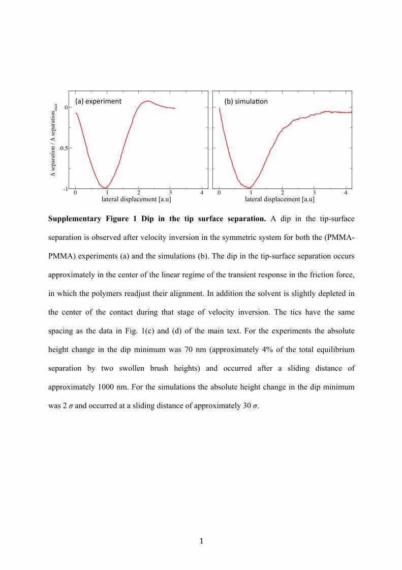
Supplementary Figure 1 Dip in the tip surface separation. A dip in the tip-surface

separation is observed after velocity inversion in the symmetric system for both the (PMMA-

PMMA) experiments (a) and the simulations (b). The dip in the tip-surface separation occurs

approximately in the center of the linear regime of the transient response in the friction force,

in which the polymers readjust their alignment. In addition the solvent is slightly depleted in

the center of the contact during that stage of velocity inversion. The tics have the same

spacing as the data in Fig. 1(c) and (d) of the main text. For the experiments the absolute

height change in the dip minimum was 70 nm (approximately 4% of the total equilibrium

separation by two swollen brush heights) and occurred after a sliding distance of

approximately 1000 nm. For the simulations the absolute height change in the dip minimum

was 2 σ and occurred at a sliding distance of approximately 30 σ.

0 1 2 3 4distance / (d2-d1)

-1

-0.5

0

6 se

para

tion

/ 6 se

para

tion m

ax0 1 2 3 4

distance / (d2-d1)

-1

-0.5

0

6 se

para

tion

/ 6 se

para

tion m

ax

lateral displacement [a.u] lateral displacement [a.u]

(a)$experiment$ (b)$simula1on$

  2  

Supplementary Figure 2 Transient response after velocity inversion asymmetric system.

The measured (a) and simulated (b) force traces for the asymmetric system. The experimental

force traces are flattened after the transient response.

0 10 20 30 40-0.02

0

0.02

F / F

sssymm

0 10 20 30 40-0.02

0

0.02

F / F

sssymm

(a)$experiment$

(b)$simula1on$

lateral displacement

  3  

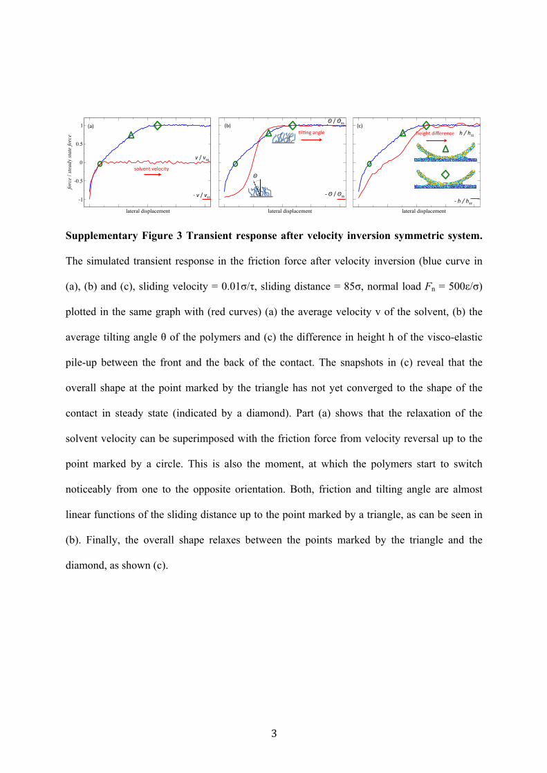
Supplementary Figure 3 Transient response after velocity inversion symmetric system.

The simulated transient response in the friction force after velocity inversion (blue curve in

(a), (b) and (c), sliding velocity = 0.01σ/τ, sliding distance = 85σ, normal load Fn = 500ε/σ)

plotted in the same graph with (red curves) (a) the average velocity v of the solvent, (b) the

average tilting angle θ of the polymers and (c) the difference in height h of the visco-elastic

pile-up between the front and the back of the contact. The snapshots in (c) reveal that the

overall shape at the point marked by the triangle has not yet converged to the shape of the

contact in steady state (indicated by a diamond). Part (a) shows that the relaxation of the

solvent velocity can be superimposed with the friction force from velocity reversal up to the

point marked by a circle. This is also the moment, at which the polymers start to switch

noticeably from one to the opposite orientation. Both, friction and tilting angle are almost

linear functions of the sliding distance up to the point marked by a triangle, as can be seen in

(b). Finally, the overall shape relaxes between the points marked by the triangle and the

diamond, as shown (c).

0 1 2 3 4

distance [a.u]0 1 2 3 4

distance [a.u]0 1 2 3 4

distance [a.u]

-1

-0.5

0

0.5

1

forc

e / s

tead

y st

ate

forc

e

!"v"/"vss"

"v"/"vss"

solvent"velocity"

.l.ng"angle"

Θ"/"Θss"

#$Θ"/"Θss"

$$Θ""

#$h$/$hss$

$h$/$hss$

lateral displacement lateral displacement lateral displacement

(a)" (b)" (c)"height"difference"

  4  

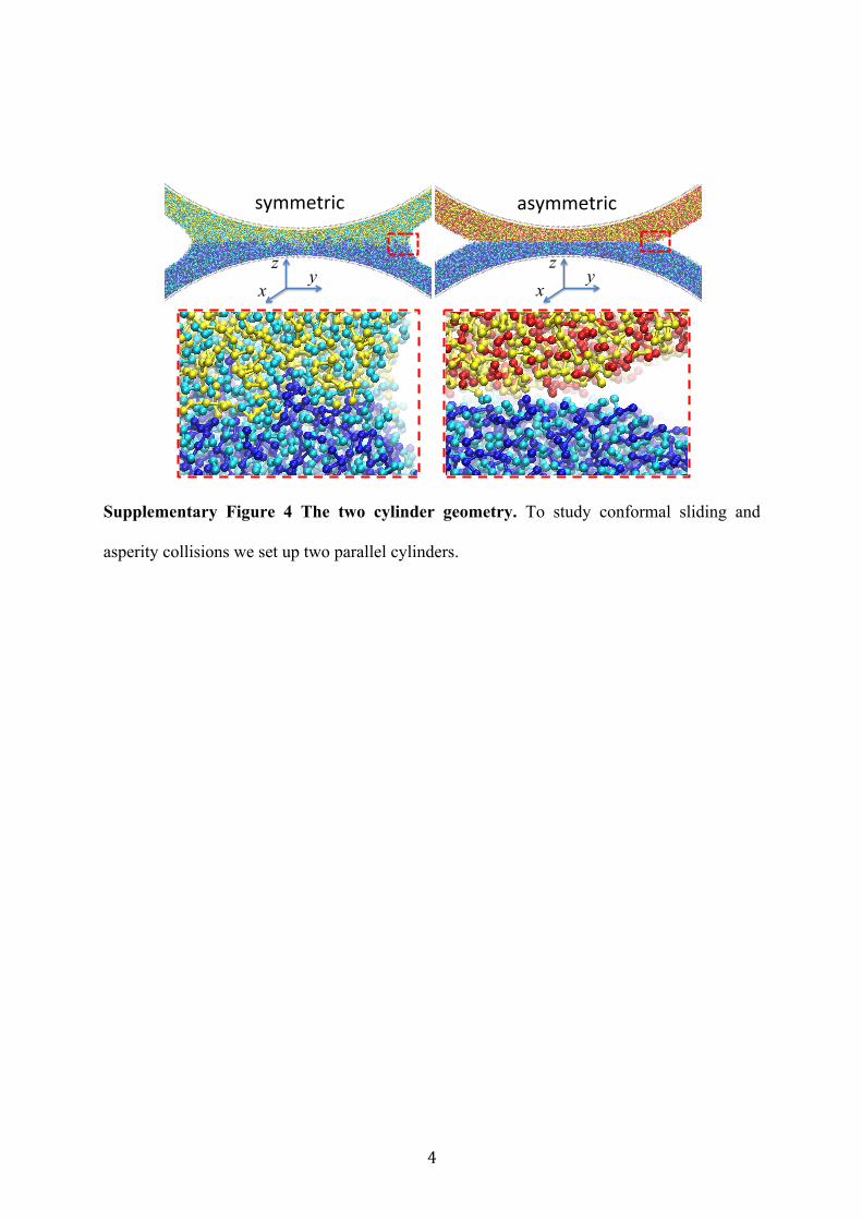
Supplementary Figure 4 The two cylinder geometry. To study conformal sliding and

asperity collisions we set up two parallel cylinders.

!"##$%&'() *!"##$%&'()

z y

x

z y

x

  5  

Supplementary Figure 5 The friction forces for the symmetric and asymmetric system in

long term measurements. The symmetric system consists out of two PNIPAM brushes. The

asymmetric system consists of a PNIPAM brush (colloid) on a PMMA brush-covered surface.

The brushes are fully solvated. The friction reduction remains approximately two orders of

magnitude. Over 4 hours, the force for the symmetric system slowly decreases. We believe

this is due to wear: The chain pullout decreases the grafting density and reduces the friction

forces. The friction force for the asymmetric system slowly increases. We believe this is due

to the slow evaporation of acetophenone from the PMMA brush.

  6  

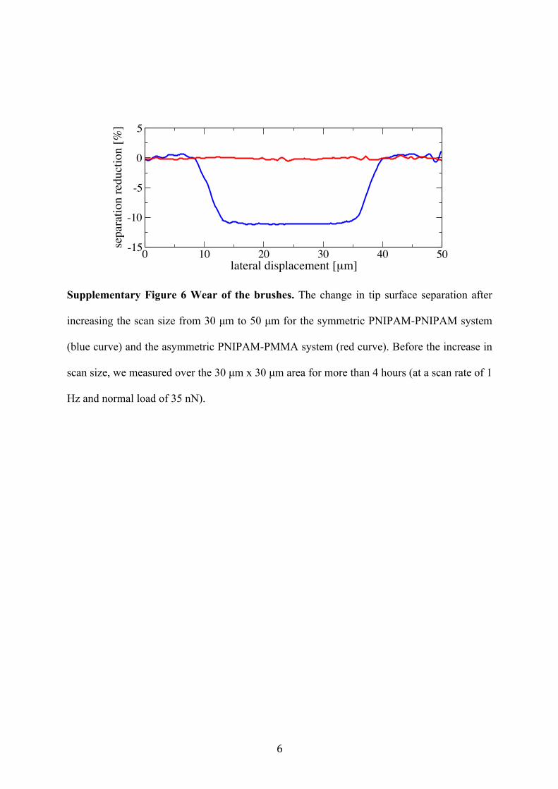
Supplementary Figure 6 Wear of the brushes. The change in tip surface separation after

increasing the scan size from 30 µm to 50 µm for the symmetric PNIPAM-PNIPAM system

(blue curve) and the asymmetric PNIPAM-PMMA system (red curve). Before the increase in

scan size, we measured over the 30 µm x 30 µm area for more than 4 hours (at a scan rate of 1

Hz and normal load of 35 nN).

0 10 20 30 40 50lateral displacement [µm]

-15

-10

-5

0

5se

para

tion

redu

ctio

n [%

]

  7  

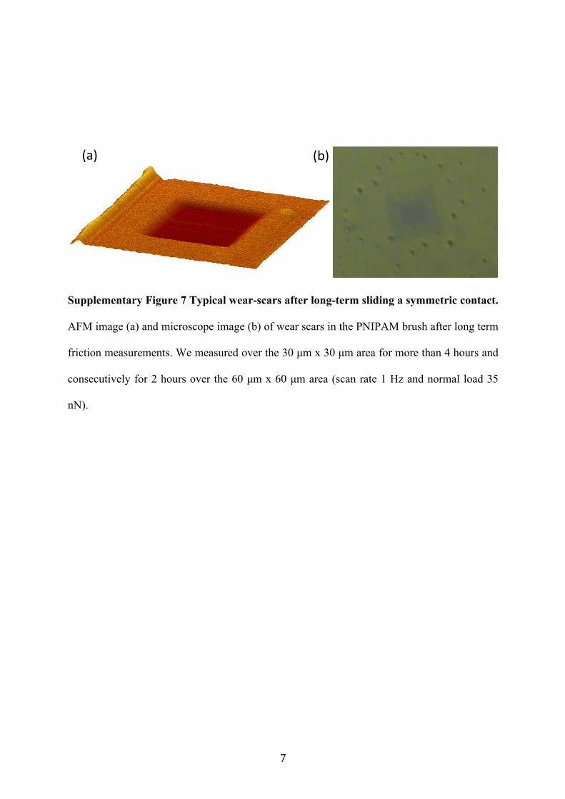
Supplementary Figure 7 Typical wear-scars after long-term sliding a symmetric contact.

AFM image (a) and microscope image (b) of wear scars in the PNIPAM brush after long term

friction measurements. We measured over the 30 µm x 30 µm area for more than 4 hours and

consecutively for 2 hours over the 60 µm x 60 µm area (scan rate 1 Hz and normal load 35

nN).

!"#$ !%#$

  8  

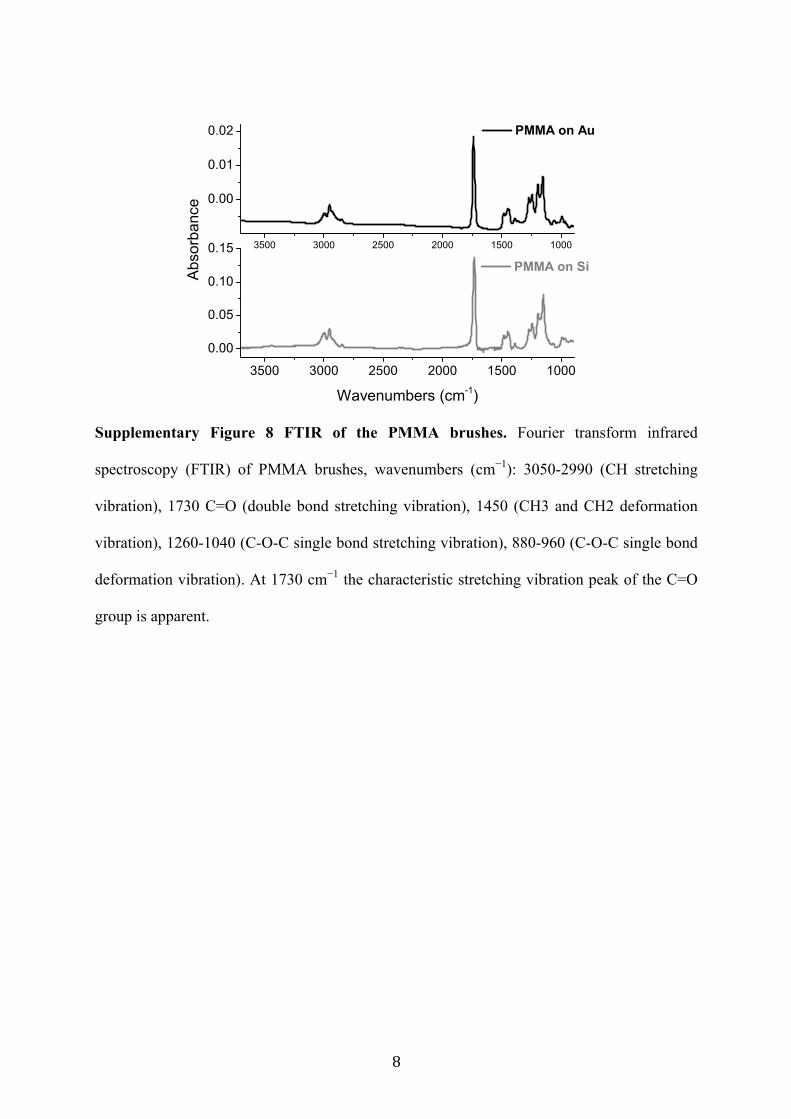
Supplementary Figure 8 FTIR of the PMMA brushes. Fourier transform infrared

spectroscopy (FTIR) of PMMA brushes, wavenumbers (cm−1): 3050-2990 (CH stretching

vibration), 1730 C=O (double bond stretching vibration), 1450 (CH3 and CH2 deformation

vibration), 1260-1040 (C-O-C single bond stretching vibration), 880-960 (C-O-C single bond

deformation vibration). At 1730 cm−1 the characteristic stretching vibration peak of the C=O

group is apparent.

3500 3000 2500 2000 1500 1000

0.00

0.01

0.02 PMMA on Au

3500 3000 2500 2000 1500 1000

0.00

0.05

0.10

0.15 PMMA on SiA

bsorbance

Wavenumbers (cm-1)

  9  

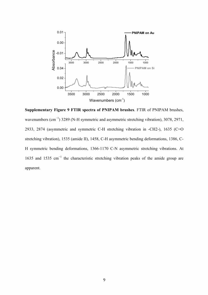
Supplementary Figure 9 FTIR spectra of PNIPAM brushes. FTIR of PNIPAM brushes,

wavenumbers (cm−1) 3289 (N-H symmetric and asymmetric stretching vibration), 3078, 2971,

2933, 2874 (asymmetric and symmetric C-H stretching vibration in -CH2-), 1635 (C=O

stretching vibration), 1535 (amide II), 1458, C-H asymmetric bending deformations, 1386, C-

H symmetric bending deformations, 1366-1170 C-N asymmetric stretching vibrations. At

1635 and 1535 cm−1 the characteristic stretching vibration peaks of the amide group are

apparent.

3500 3000 2500 2000 1500 1000

-0.01

0.00

0.01 PNIPAM on Au

3500 3000 2500 2000 1500 1000

0.00

0.02

0.04 PNIPAM on SiAbsorbance

Wavenumbers (cm-1)

  10  

Supplementary Notes

To put ourselves into a position in which we can rightfully compare experiment and

simulation, we tried to match dimensionless numbers as well as possible rather than to make

selected parameters identical. The rational is that dimensionless numbers predominantly

determine responses in fluid mechanics. Unfortunately, one can essentially only dispose of

two parameters in the experiments, i.e, the degree of polymerization P, and the grafting

density α, once a specific chemistry is identified. We chose them such that the Weissenberg

number W, i.e, the product of shear rate γ and the characteristic relaxation time τ would be of

similar order of magnitude. We also tried to keep the geometry, charaterized by the ratio of

brush height and radius of curvature, similar. A third parameter is the swelling ratio, which is

the swollen brush height normalized by the dry brush height. In the experimental system, the

ratio of swollen and unswollen brush is a little greater than three. In the simulations, the

swelling ratio is approximately 2.6. The detailed rational for the choices of grafting densities

and chain lengths can be summarized as follows: Firstly, experiments are done at much

smaller velocities and much smaller shear rates γ than the simulations. They deviate by

approximately four decades. Thus, in order to roughly match the Weissenberg number W

between simulation and experiment, we needed to set up experimental systems with

correlation times exceeding those of the in-silico brushes by a similar factor. This could be

achieved by using large degrees of polymerization. To make a crude estimate, we pursue as

follows: Polymer brushes have a spectrum of relaxation times1. For interdigitation, the

relevant relaxation time and thus W scales as γ(η(kBT)-1)P2.31(αg/d)0.31, where η is the solvent

viscosity, T is the temperature, P is the degree of polymerization, αg is the grafting density,

and d is the distance between the chains2. Thus, we can calculate the ratio Wexp/Wsim = 0.21.

Even if our calculations are off by one decade, we would argue that we targeted the

Weissenberg sufficiently well, as we see no qualitatively different results in the simulations

  11  

when changing shear rates by one decade in either direction. Secondly, we tried to keep the

geometric ratio R/L0 (R is tip radius and L0 is the swollen brush height) constant. For the

experiments and simulations described in the main text, we had R/L0 = 6 and R/L0 = 5,

respectively. In addition, all fluids are low viscosity solvents. Thus, the solvents should

always respond reasonably fast to changes and the polymers be much slower.

One parameter that turned out different between simulations and experiments is the Tabor

coefficient, µT, which is a dimensionless measure for how long-ranged interactions are.

Specifically, we associate a short-range interaction (or in the language of Hertzian contact

mechanics a JKR-like contact) with the experimental systems, in particular for the symmetric

contacts. Therefore, we found a weaker increase of the friction force on the normal load in the

experiments than in the simulations. Yet, the differences between JKR and DMT like contacts

are relatively subtle, i.e., prefactors and exponents describing displacement-load curves differ

by no more than O(30%). This is why one can expect that exponents differ for laboratory and

in-silico brushes, but trends will be similar.

  12  

Supplementary Methods

The experimental data is averaged over 70-150 force traces, symmetrized and small residual

oscillations (due to interference of the laser-light) are filtered out by fitting and subtracting a

cosine with a separation- dependent phase-shift. Moreover, the first 100 force traces are

discarded. In the simulations, 5 force traces were needed to equilibrate the system.

We discussed in the main text, that for the symmetric system both the simulated and the

measured transient response after velocity-inversion can be fitted with an empirical shape

function that consists of an exponential relaxation, a linear regime and an exponential

relaxation to the steady state force. The 3 different regimes are connected via a Heaviside

function θ(x), where θ(x < 0) = 0, θ(x > 0) = 1 and θ(x = 0) = 0.5. This results in the following

fit-function:

F = −Fss exp (−x/λ1) θ(X1−x) + (Ax+B) θ(x−X1) θ(X2−x) + Fss(1−Cexp(−x/λ2) θ(x−X2),

in which Fss is the steady state force, x is the sliding distance, λ1 and λ2 are the first and second

relaxation distance resp., A sets the slope of the linear regime, B the crossing with the y-axis

for the linear regime, C the decay of the final exponential relaxation and X1 and X2 are the

distances at which we link regime 1 to 2 and 2 to 3 resp.. By normalizing the measured or

simulated force by Fss and the sliding distance by, e.g. λ1, we are left with 6 fitting

parameters. By imposing that at X1 and X2 the function and its derivative should be

continuous, we can eliminate 4 more parameters, such that 2 independent fitting parameters

remain. At the highest simulation velocities (v > 0.01σ/τ) not all data perfectly matched the

shape function. For these datasets an extra fitting parameter is introduced by replacing the

function for the initial relaxation by −Fss + D (1 − exp (−x/λ1)), such that the final value of the

initial relaxation can be different from 0.

  13  

Supplementary References

1. de Beer, S. and Müser, M. H. Alternative dissipation mechanisms and the effect of the

solvent in friction between polymer brushes on rough surfaces, Soft Matter 9, 7234-7241

(2013).

2. Spirin, L., Galuschko, A., Kreer, T., Johner, A., Baschnagel, J. and Binder, K., Polymer-

brush lubrication in the limit of strong compression, Eur. Phys. J. E 33, 307-311 (2010).