A Fast Band–Krylov Eigensolver for

Macromolecular Functional Motion Simulation on

Multicore Architectures and Graphics Processors

Jose I. Aliagaa,∗, Pedro Alonsob, Jose M. Badıaa, Pablo Chaconc,Davor Davidovicd, Jose R. Lopez–Blancoc, Enrique S. Quintana-Ortıa

aDepto. Ingenierıa y Ciencia de Computadores, Universitat Jaume I, Castellon, SpainbDepartamento de Sistemas Informaticos y Computacin,

Universitat Politecnica de Valencia, SpaincDept. Biological Chemical Physics, Rocasolano Physics and Chemistry Institute,

CSIC, Madrid, SpaindInstitut Rudjer Boskovic, Centar za Informatiku i Racunarstvo - CIR, Zagreb, Croatia

Abstract

We introduce a new iterative Krylov subspace-based eigensolver for the simu-lation of macromolecular motions on desktop multithreaded platforms equippedwith multicore processors and, possibly, a graphics accelerator (GPU). Themethod consists of two stages, with the original problem first reduced intoa simpler band-structured form by means of a high-performance compute-intensive procedure. This is followed by a memory-intensive but low-costKrylov iteration, which is off-loaded to be computed on the GPU by meansof an efficient data-parallel kernel.

The experimental results reveal the performance of the new eigensolver.Concretely, when applied to the simulation of macromolecules with a fewthousands degrees of freedom and the number of eigenpairs to be computedis small to moderate, the new solver outperforms other methods implementedas part of high-performance state-of-the-art packages for multithreaded ar-chitectures.

∗Corresponding authorEmail addresses: aliaga@uji.es (Jose I. Aliaga), palonso@dsic.upv.es

(Pedro Alonso), badia@uji.es (Jose M. Badıa), pablo@chaconlab.org (Pablo Chacon),ddavid@irb.hr (Davor Davidovic), jrlopez@iqfr.csic.es (Jose R. Lopez–Blanco),quintana@uji.es (Enrique S. Quintana-Ortı)

Preprint submitted to Journal of Computational Physics September 28, 2015

Significance and Novelty of this paper

Keywords: Computational biology, macromolecular machines, eigenvalueproblems, Krylov subspace methods, multicore processors, graphicsprocessors

Significance and Novelty of this paper

In this paper we further enhance the appeal of the Krylov subspace-basedmethods to model the functional motions of large-scale macromolecular ma-chines. We introduce a new iterative solver that combines an initial trans-formation of the original data into band-structured problem, followed by theclassical Krylov iteration applied to this reduced problem. There are twoadvantages of the new “band-Krylov” method:

1. It transfers a large fraction of the iteration cost into the initial, efficientreduction to band form.

2. Subsequently, it applies the low-performance Krylov iteration on asmaller problem which implies a lower cost of this stage and, addition-ally, the possibility of accommodating the data closer to the processorfloating-point units (FPUs).

For the second stage, as an additional contribution of this work, we developan efficient implementation of a symmetric band matrix-vector product thatsignificantly accelerates the computation of the Krylov iteration on a graphicsprocessor unit (GPU).

The results with large-scale macromolecules, featuring several tens ofthousands DOFs, show that combination of these three factors (reductionto band form, iterative procedure with the reduced band matrix, and accel-eration of the iteration by means of a fast GPU kernel) offers a more efficientsolution. The figures expose the advantages of the new band-Krylov solvercompared with the original “full-Krylov” method as well as the methodsincluded in state-of-the-art libraries for high-performance multicore serverswith or without GPUs. Moreover, the new band–Krylov solver can handlelarger problems on the GPU, as the initial reduction to band form can be per-formed out-of-core from the perspective of the accelerator, while the Kryloviteration proceeds in-core on a band matrix of reduced size.

2

A Fast Band–Krylov Eigensolver for

Macromolecular Functional Motion Simulation on

Multicore Architectures and Graphics Processors

Jose I. Aliagaa, Pedro Alonsob, Jose M. Badıaa, Pablo Chaconc,Davor Davidovicd, Jose R. Lopez–Blancoc, Enrique S. Quintana-Ortıa

aDepto. Ingenierıa y Ciencia de Computadores, Universitat Jaume I, Castellon, SpainbDepartamento de Sistemas Informaticos y Computacin,

Universitat Politecnica de Valencia, SpaincDept. Biological Chemical Physics, Rocasolano Physics and Chemistry Institute,

CSIC, Madrid, SpaindInstitut Ruder Boskovic, Centar za Informatiku i Racunarstvo - CIR, Zagreb, Croatia

Abstract

We introduce a new iterative Krylov subspace-based eigensolver for the simu-lation of macromolecular motions on desktop multithreaded platforms equippedwith multicore processors and, possibly, a graphics accelerator (GPU). Themethod consists of two stages, with the original problem first reduced intoa simpler band-structured form by means of a high-performance compute-intensive procedure. This is followed by a memory-intensive but low-costKrylov iteration, which is off-loaded to be computed on the GPU by meansof an efficient data-parallel kernel.

The experimental results reveal the performance of the new eigensolver.Concretely, when applied to the simulation of macromolecules with a fewthousands degrees of freedom and the number of eigenpairs to be computed issmall to moderate, the new solver outperforms other methods implemented aspart of high-performance numerical linear algebra packages for multithreadedarchitectures.

Keywords: Computational biology, macromolecular machines, eigenvalueproblems, Krylov subspace methods, multicore processors, graphicsprocessors

Preprint submitted to J. Computational Physics September 28, 2015

*ManuscriptClick here to view linked References

1. Introduction

Living cells consist of long chains of aminoacids and nucleotides, usu-ally assembled into large macromolecular machines that support the mainbiological functions. At the molecular level, the biological activity of thesecomponents can be studied via Molecular Dynamics (MD) simulations oftheir dynamics and interactions. These studies provide detailed informationon the fluctuations and conformational changes of protein and nucleic acidsmacromolecules using available 3D atomic structures. Unfortunately, thelarge size of these macromolecules and the long time scale of their motionturn MD simulations too costly or even prohibitive in practice.

Coarse-grain (CG) models combined with normal mode analysis (NMA)compose a powerful alternative to simulate collective motions of macromolec-ular complexes at extended time scales [1, 2]. For example, the experimentsin [3, 4, 5, 6, 7, 8] demonstrate that CG-NMA can efficiently model molecu-lar flexibility, thus becoming an appealing alternative for expensive atomisticsimulations. Moreover, reformulating NMA in internal coordinates (ICs) [9]greatly reduces the number of degrees of freedom (DOF), extending the ap-plicability of NMA to even larger macrocomplexes.

The diagonalization of a large-scale matrix pair (i.e., the solution ofa generalized eigenproblem) is the most expensive operation in IC-NMA.In [10] we compared two approaches to compute a fraction of the spectrumof moderate-scale dense symmetric definite generalized eigenproblems, basedrespectively on the reduction to tridiagonal form and the Krylov subspace it-eration. In [11] we particularized this analysis for molecular dynamics (MD)simulations, showing that the iterative Krylov subspaces are an attractive so-lution for large-scale macromolecules, with up to 150,000 degrees of freedom(DOFs), when tackled on a cluster of multicore processors.

In this paper we further enhance the appeal of the Krylov subspace-basedmethods by introducing a new iterative solver that combines an initial trans-formation of the original data into band-structured problem, followed by theclassical Krylov iteration applied to this reduced problem. The advantagesof the new “band-Krylov” method lie in that i) it transfers a large fractionof the iteration cost into the initial, efficient reduction to band form; and ii)it then operates the low-performance Krylov iteration on a smaller problemwhich implies a lower cost of this stage and, additionally, the possibility ofaccommodating the data closer to the processor floating-point units (FPUs).For the second stage, as an additional contribution of this work, we develop

2

an efficient implementation of a symmetric band matrix-vector product thatsignificantly accelerates the computation of the Krylov iteration on a graphicsprocessing unit (GPU).

Overall, we expect that the combination of these three factors (fast andefficient reduction to band form, iterative procedure with the reduced bandmatrix, and acceleration of the iteration by means of a fast GPU kernel)offers a more efficient solution for moderate- to large-scale problems as thenumber of iterations required for convergence grows. The results with large-scale macromolecules, featuring several tens of thousands DOFs, expose theadvantages of the new band-Krylov solver compared with the original “full-Krylov” method as well as the methods included in linear algebra librariesfor high-performance multicore servers with or without GPUs.

The rest of the paper is structured as follows. In Section 2 we summarizethe principles behind macromolecular motion simulation in internal coordi-nates, identifying the key numerical problem appearing in this approach. InSection 3 we revisit some popular numerically-stable methods for the solutionof eigenvalue problems, and we provide a list of existing libraries and pack-ages that implement these methods for current multicore architectures andGPUs. This section also discusses the properties of these methods from thepoint of view of computational cost and performance, motivating the intro-duction of the new fast cache-efficient band–Krylov eigensolver in Section 4.The experimental results follow in Section 5 using a recent hybrid platformconsisting of a 6-core Intel Xeon “Sandy Bridge” processor, connected toan NVIDIA “Kepler” graphics card. Finally, the paper is closed with a fewconcluding remarks in Section 6.

2. Capturing Macromolecular Dynamics in Internal Coordinates

Macromolecular motions can be described in normal mode analysis (NMA)by approximating the potential (Hessian) and kinetic energies as quadraticfunctions of the atomic positions and velocities, respectively. This in turn al-lows the decomposition of the motion into a series of vectors that encode thepotential displacement directions and can be obtained from the modes (i.e.,the eigenvalues) of the second derivative of the potential and kinetic energymatrices. The low frequency modes, in particular, correspond to soft collec-tive conformational changes, which are related to functional motions [12, 13],and feature a close relation with atomistic MD [14, 15, 16].

3

iMod [9] exploits classical NMA formulations in internal coordinates(ICs) while extending them to model large-scale macromolecular structures.In this representation, the potential energy of the system is expressed as

A =1

2q HqT , (1)

where the vector q contains the displacement from the equilibrium confor-mation (q = qe − q0);

H = (Hα,β) =∂2V

∂qα∂qβ(2)

is the Hessian matrix; and the α and β subindices represent any IC to com-pute the partial derivatives. Furthermore,

V =∑i<j

Fij(reij − r0ij)2, (3)

where Fij is the spring stiffness matrix, and rij denotes the distance betweenatoms i and j.

Additionally, the kinetic energy is given by:

B =1

2q T qT , (4)

where q = d q/dt, and the kinetic energy matrix is defined as

T = (Tα,β) =∑i

mi∂ri∂qα· ∂ri∂qβ

. (5)

Here, the mass of the i-th atom is mi, while ri stands for the correspondingCartesian position vector. In general, the solution of the Lagrange equationof motion (L = T − V ) can be encoded in the lowest frequency componentsof the eigenproblem defined by the matrix pair (A,B); see [11] for details.

3. Solution of Symmetric Definite Eigenproblems

The IC-NMA method described in Section 2 requires the solution of ageneralized symmetric definite eigenproblem of the form

AX = BXΛ, (6)

4

where A ∈ Rn×n and B ∈ Rn×n are both dense symmetric positive definite,corresponding respectively to the Hessian and kinetic energy matrices thatcontrol the dynamics of the macromolecular complex; Λ ∈ Rs×s is a diagonalmatrix with the s sought-after smallest eigenvalues (or modes) of the matrixpair (A,B) on its diagonal entries; and the columns of X ∈ Rn×s containthe associated unknown eigenvectors [17]. Furthermore, for accurate macro-molecular motion simulation n ≥ 10,000, but typically only the s smallesteigenpairs (i.e., the eigenvalues and eigenvectors for the low energy modes)are necessary, with s ≈ 2–10% of n.

Numerically-reliable eigensolvers for (6) initially transform this general-ized equation into a standard symmetric eigenproblem:

CY = Y Λ, (7)

where C = U−TAU−1 ∈ Rn×n is symmetric, Y = UX ∈ Rn×s, and U ∈ Rn×n

is the Cholesky factor of B (i.e., B = UTU with U upper triangular) [17].Thus, the standard eigenproblem (7) shares its eigenvalues with those of (6),while the original eigenvectors can be easily recovered from X = U−1Y ,which only requires the solution of a few triangular linear system.

Since all the methods described next share the initial transformation intoa standard eigenvalue problem and the back-transform to obtain the originaleigenvectors, we will omit these two operations from the following discussion.

3.1. Direct eigensolvers

A popular approach to solve (7) commences by initially reducing C to asymmetric tridiagonal matrix T ∈ Rn×n via an eigenvalue-preserving simi-larity transform:

QTCQ = T, (8)

defined by the orthogonal matrix Q ∈ Rn×n. This is followed by a subse-quent refinement to extract the eigenvalues from the associated symmetrictridiagonal eigenproblem:

TZ = ZΛ, (9)

where Z ∈ Rn×s comprises the sought-after eigenvectors of T . Finally, theeigenvectors of the standard problem are recovered from Y = QZ. Fromthe numerical perspective, the most involved part of this approach is thesolution of the tridiagonal eigenproblem (9), which can be reliably tackled,e.g., via the QR algorithm or the MRRR method [17], both available as

5

part of LAPACK [18]. On the other hand, from the computational pointof view, the most expensive component in terms of floating-point arithmeticoperations (flops) is the reduction of C to tridiagonal form (8). In particular,this reduction costs O(n3) flops while, in general, the subsequent solution ofthe tridiagonal eigenproblem only requires O(n2) flops [17]. Recovering Yfrom Z only adds O(n2s) flops to these figures.

We next describe two alternative approaches to obtain the tridiagonalmatrix T and the associated orthogonal factor Q, and refer to numericalsoftware packages for this purpose.

3.1.1. One-stage reduction to tridiagonal form

LAPACK’s routine sytrd performs the transformation (8) in a sin-gle stage via Householder reflectors. Specifically, at a given iteration j =1, 2, . . . , n− 2, this procedure computes a reflector Hj that annihilates all el-ements below the first subdiagonal of the j-th column of the current matrixC(j−1), with C(0) = C, accumulating this transform as

C(j) = HTj C

(j−1)Hj = HTj (HT

j−1HTj−2 · · ·HT

1 CH1 · · ·Hj−1) Hj, (10)

so that Q = H1 · · ·Hn−3Hn−2 yields the desired reduction in (8). To attainhigh performance, the application of these reflectors is partially delayed, ag-gregating groups of b (block size) transforms, so as to permit a more efficientupdate of C via a blocked algorithm [17]. The overall cost of performingthe reduction (8) using routine sytrd is 4n3/3 flops, provided b n. Fur-thermore, the back-transform Y = QZ can be computed using LAPACK’sroutine ormtr, at a cost of 2n2s additional flops, without ever forming Q.

Following the traditional approach, the LAPACK routines for this proce-dure extract parallelism for (general-purpose) multicore processors by rely-ing on a multithreaded implementation of BLAS. Alternative multithreadedimplementations of these procedures have been recently proposed for (many-core) GPUs as part of the MAGMA [19] library.

3.1.2. Multi-stage reduction to tridiagonal form

The problem with the one-stage reduction just described is that half ofthe flops performed by routine sytrd are cast in terms of the symmetricmatrix-vector product (symv), which delivers a small fraction of the peakperformance on current multicore and manycore architectures.

6

The multi-stage methods shift a major part of the computations necessaryfor the reduction into symmetric rank-2b updates (syr2k), basically equiv-alent to the efficient matrix-matrix product. In exchange, these methodsincur a considerable increase of the computational cost. Let us consider, forsimplicity, a two-stage algorithm. The idea is to initially transform C intoa symmetric band matrix W ∈ Rn×n, with bandwidth w, via an orthogonalsimilarity transform Q1, to then further reduce W into the tridiagonal ma-trix T using an additional orthogonal similarity transform Q2. The first stagemostly consists of fast rank-2b stages, while the type of operations appearingin the second stage are the same as those in the slow reduction to tridiagonalform. Provided w n, this two-stage calculation of T roughly costs 4n3/3flops, i.e., the same as the one-stage algorithm. However, the constructionof the orthogonal matrix Q = Q1Q2 that performs the full transformationQT

2 (QT1CQ1)Q2 = QT

2WQ2 = T , necessary to recover the eigenvectors of Yfrom those of Z, becomes considerably more expensive, requiring 2n3 + 2n2sadditional flops.

There exists a complete implementation of the two-stage method in theSBR toolbox [20], which can leverage a multithreaded implementation ofBLAS to exploit the hardware concurrency of current multicore processors.For these same architectures one can also leverage the codes in the PLASMAlibrary [21]. A reimplementation of this approach to tackle large-scale prob-lems, which do not fit into the memory of the GPU, was done in [22].ELPA [23] and MAGMA [24] implement a variant of the two-stage method,for clusters and multi-GPU platforms, respectively. Both implementationsexhibit significantly lower computational cost compared with the originalSBR algorithm, but they are still significantly more expensive than the one-stage approach.

3.2. Iterative (Krylov subspace-based) eigensolvers

Alternatively, the solution of symmetric eigenproblems can be tackled bymeans of a Krylov subspace-based method [17], an inexpensive choice for thesolution of large-scale dense eigenproblems on multicore architectures andGPUs [25].

When applied to C, starting from an initial random vector v1 ∈ Rn, allKrylov subspace-based methods construct a basis of the Krylov subspacespanned by this matrix, defined as

K(C, v1, n) = spanv1, Cv1, . . . , Cn−1v1 = spanv1, v2, . . . , vn. (11)

7

If C is symmetric and positive definite, this matrix can be reduced to tridiago-nal form via similarity orthonormal transform defined by V = [v1, v2, . . . , vn];i.e.,

V TCV = T =

α1 β1 0

β1 α2. . .

. . . . . . βn−1

0 βn−1 αn

, V TV = I. (12)

Thus, equating the columns in CV = V T , the Lanczos three-term recurrenceis obtained

Cvk = βk−1vk−1 + αkvk + βkvk+1, (13)

with β0v0 = 0. Given the orthonormality of V , and operating properly on therecurrence, we obtain the expressions to compute the components of matrixT , which are the foundation of the Lanczos method:

αk = vTkAvk,rk = βkvk+1 = (C − αkI)vk − βk−1vk−1,βk = ||rk||2

(14)

such that the reduction in the m-th iteration is given, in matrix form, by

CVm = VmTm + rmeTm (15)

This method exhibits low computational cost per iteration (in general, 2n2

flops) and, moreover, does not require an appreciable additional storagespace. But the main feature of the Lanczos method is that the extremaleigenvalues of matrix Tm are good approximation of the extremal eigenval-ues of matrix C, specially if there are not clustered, improving this conditionwhen m increases. Empirically, it has been proved that if the number ofsought-after eigenvalues of C is equal to s the size of the Krylov subspace hasto be m ≥ 2s. For macromolecular simulations it is convenient to computethe largest s eigenvalues of the pair (B,A), instead of the smallest s eigen-values of the correlated problem (A,B) as, for these particular applications,the former have the appealing property of being extremal and well-separated,ensuring fast convergence of the iteration.

Krylov subspace methods are implemented as part of ARPACK [26]. Thisnumerical package features a “reverse communication” interface so that theuser is in charge of providing an efficient implementation of symv. We note

8

that this is the only operation that “interacts” with the matrix in ARPACK,concentrating the bulk of the operations performed in this library. Efficientimplementations of symv are offered as part of most tuned implementationsof BLAS, including Intel MKL for multicore processors and CUBLAS forGPUs.

3.3. Discussion of existing methods

The methods described in the previous two subsections present a numberof advantages and drawbacks that we next review in order to motivate ouralternative solver.

The algorithms based on the two-stage (or multi-stage) reduction to tridi-agonal form are mostly composed of compute-bound kernels (concretely, thelevel 3 BLAS syr2k) which, in general, attain very high performance on cur-rent multicore and manycore architectures. However, their high cost oftenturns them too expensive for the solution of eigenproblems when only a re-duced number of eigenvalues/eigenvectors is required [10]. A large fraction ofthis overhead is rooted in the need to explicitly build the orthogonal matrixQ, which requires the additional 2n3 flops.

On the other hand, the one-stage reduction to tridiagonal form avoidsthe explicit construction of the orthogonal matrix, offering a much reducedcomputational cost compared with its two-stage counterparts. Nevertheless,half of the operations in this method are cast in terms of a memory-boundkernel (specifically, the level 2 BLAS symv), which offers very low perfor-mance in today’s architectures. Furthermore, the method incurs in the samecost independently of the number of eigenvalues that are required (4n3/3flops to reduce C to T ), though the eigenvectors can be computed at a costthat is proportional to their number (2n2s flops to obtain Y from Z).

The Krylov subspace methods perform the bulk of its computations interms of the memory-bound symv, and therefore can be expected to achieveonly a small fraction of the processor’s peak performance. On the positiveside, they are often the cheapest methods, with a cost of roughly 2n2 flopsper iteration and a fast convergence rate for macromolecular motion simula-tions [11].

Consider the symv y = Cx, where C ∈ Rn×n is symmetric and x, y ∈ Rn,and let us denote the (i, j) entry of C by ci,j and the k-th entry of x/y asxk/yk. The low-performance of this kernel is due to the fact that there isno reuse of the matrix elements. In particular, for each element of C that isbrought into the FPUs, the operation performs 4 flops (yi += ci,j · xj and

9

yj += ci,j · xi), rendering a ratio of 4 flops per memory operation (memop).On current architectures, where the memory bandwidth is much lower thanthe FPUs’ peak performance, the result is a memory-bound operation thatis strongly constrained by the speed of the memory level where the data (i.e.,the matrix C) resides.

A particularly harmful scenario for the symv kernel and, in consequence,for the Krylov subspace methods (as well as the one-stage reduction to tridi-agonal form) is a problem where the data matrix C is too large to fit into themain memory and, therefore, has to be retrieved from disk at each iterationof the method. In this situation, the disk (I/O) bandwidth strictly dictatesthe performance of the Krylov subspace-based solver, while other parameterssuch as the number of cores, frequency, SIMD organization, etc. of the targetarchitecture play a minor role. Similarly, in a problem with data too large tofit into the memory of a GPU, the matrix has to be transferred from the mainmemory to the graphics accelerator, via the PCI-e bus, once per iteration ofthe Krylov solver. In these circumstances, it is the PCI-e bandwidth thatdetermines the performance of the solver, independently e.g. of the numberof cores in the GPU.

Our approach to tackle this problem consists in reducing the dimensionof the problem matrix involved in the Krylov subspace method so as to beable to fit the result closer to the FPUs, e.g. in the main memory insteadof the disk, the GPU memory instead of the main memory, or the L3 cacheinstead of the main memory. Note that this will not improve the data reusefactor (flops to memops), but at least it will allow that the memops proceedat the speed of a faster memory level.

4. A Fast Cache-Efficient Band–Krylov Eigensolver

Our new iterative algorithm is a “mixed” band–Krylov method that ini-tially performs a reduction of C to a symmetric band matrix W , much likethe two-stage direct eigensolver, to then apply a Krylov subspace method onthe reduced problem.

Concretely, the new method commences by transforming the standardproblem into a symmetric band one:

W Y = Y Λ (16)

where QTCQ = W is an orthogonal similarity transform that produces theband matrix W , and Y = QY . A major difference with the two-stage direct

10

approach is that, in the direct case, the bandwidth of W was chosen to besmall (usually, around 128–256, depending on the target architecture) so asto decrease the number of flops in the subsequent stage (low-performancereduction of band to tridiagonal form) while still ensuring high performanceduring the first stage.

Our goal and, consequently, our approach differs in that we choose thebandwidth w as large as possible, with the only limitation that the resultingband matrix W , when stored in compact form as an n×(w+1) dense matrix,fits into the “target” memory level. The cost for this initial reduction is thus2((n− w)2w + (n− w)3/3) flops, which are cast in terms of efficient Level 3BLAS kernels. (Compare it with the 4n3/3 flops required for the calculationof the narrow-banded W in the direct case.)

In the second stage of our band–Krylov approach, we simply tackle thereduced problem (16) by applying a Krylov subspace-based eigensolver, witha cost of 2nw flops per iteration. Note that with this hybrid methodology, Qdoes not need to be explicitly constructed but simply applied to Y in orderto obtain the standard eigenvectors, at a cost of only 2(n−w)2s flops. Thus,compared with the original Krylov method, we reduce the cost per iterationfrom 2n2 to 2nw flops, at the expense of the initial transform to band form.On the other hand, compared with the two-stage direct method, we avoidthe costly formation of Q.

In summary, there exists a trade-off between the cost of the two stagesof our band–Krylov eigensolver and the bandwidth. Small/large values of wshift part of this cost towards/away from the initial transform but yield acheap/costly Krylov iteration. Therefore, this parameter has to be chosentaking into account the convergence rate of the Krylov method.

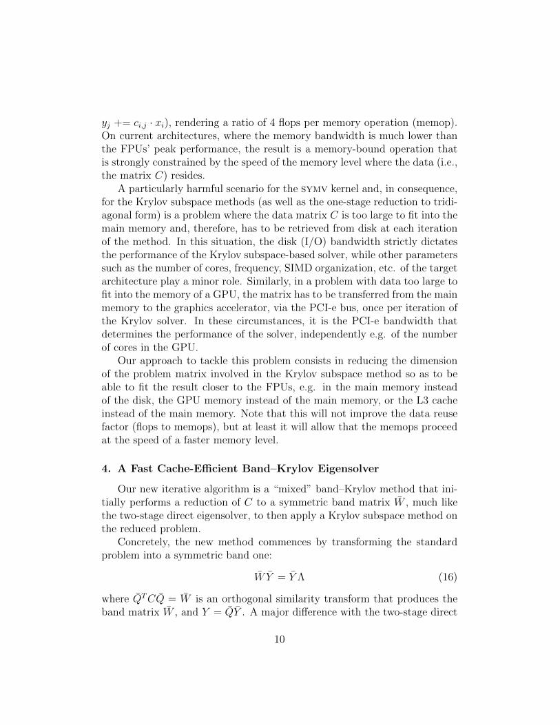
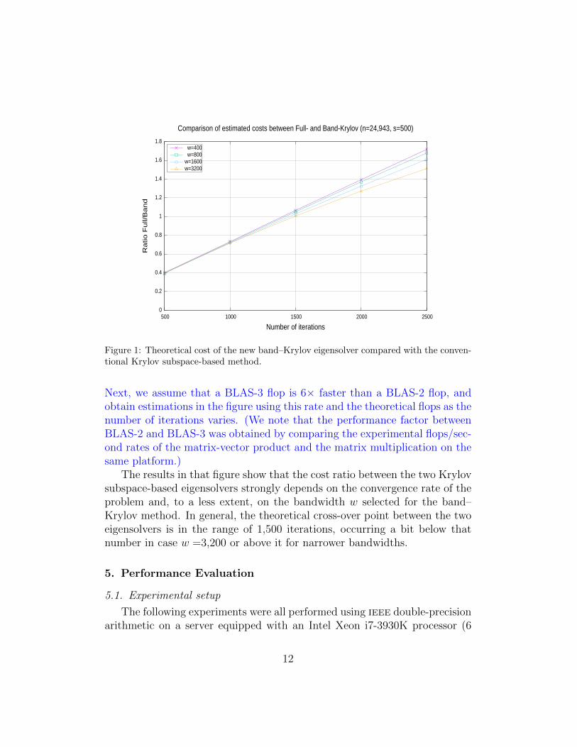
Let us illustrate this balance via the computation of the s smallest eigen-values of a random problem of “moderate” dimension n =24,943. Figure 1compares the estimated (or “expected”) cost of the full- and band-Krylovsolvers for this particular case. To perform this comparison, we consider thetheoretical number of floating-point arithmetic operations (flops) for eachsolver:

– 2n2 flops for the full-Krylov solver (all of them casted as BLAS-2 ker-nels); and

– 2((n− w)2w + (n− w)3/3) flops for the initial reduction to band form(BLAS-3 kernels), with bandwidth w, plus 2nw flops per iteration(BLAS-2 kernels), in the band-Krylov solver.

11

0

0.2

0.4

0.6

0.8

1

1.2

1.4

1.6

1.8

500 1000 1500 2000 2500

Rat

io F

ull/B

and

Number of iterations

Comparison of estimated costs between Full- and Band-Krylov (n=24,943, s=500)

w=400w=800

w=1600w=3200

Figure 1: Theoretical cost of the new band–Krylov eigensolver compared with the conven-tional Krylov subspace-based method.

Next, we assume that a BLAS-3 flop is 6× faster than a BLAS-2 flop, andobtain estimations in the figure using this rate and the theoretical flops as thenumber of iterations varies. (We note that the performance factor betweenBLAS-2 and BLAS-3 was obtained by comparing the experimental flops/sec-ond rates of the matrix-vector product and the matrix multiplication on thesame platform.)

The results in that figure show that the cost ratio between the two Krylovsubspace-based eigensolvers strongly depends on the convergence rate of theproblem and, to a less extent, on the bandwidth w selected for the band–Krylov method. In general, the theoretical cross-over point between the twoeigensolvers is in the range of 1,500 iterations, occurring a bit below thatnumber in case w =3,200 or above it for narrower bandwidths.

5. Performance Evaluation

5.1. Experimental setup

The following experiments were all performed using ieee double-precisionarithmetic on a server equipped with an Intel Xeon i7-3930K processor (6

12

cores at 3.2 GHz) and 24 GB of DDR3 RAM, connected to an NVIDIA TeslaK20 accelerator (2,496 CUDA cores at 706 MHz, with 5 GB of GDDR5 RAM)via a PCI-e 16× bus.

The codes/libraries were processed with the Intel compiler icc (compo-serve 2011 sp1.9.293, icc 12.1.3 20120212), and linked to the implemen-tation of LAPACK/BLAS implementations in Intel MKL (v10.3 update 9)and NVIDIA CUBLAS (v5.0). The MPI eigensolvers were linked to Open-MPI (1.6).

5.2. Macromolecules

For the comparison, we employ a case study corresponding to a micro-tubule (MT) 13:3 macromolecule, with three different instances, leading toeigenproblems of size n =12,469, 24,943 and 31,178. The atomic structureof MT was generated from the experimental coordinates (PDB-ID 1TUB),optimized using molecular dynamics, and kindly provided by M. Deriu [27].For details on the biological significance of these cases, see [11]. NMA wasperformed under the elastic network model approximation with iMod [9], i.e.without any further energy minimization and considering that the optimizedstructure is at the minimum energy conformation. For each one of thesecases, we compute the s = 100, 200, 300, 400, 500 and 1,000 smallest eigen-values and the associated eigenvectors of the pair (A,B). As argued earlier,in the Krylov subspace-based eigensolvers, we obtain this information fromthe s largest eigenvalues/eigenvectors of the pair (B,A).

The experimentation with other macromolecules offered similar qualita-tive results. We note that the execution time of ELPA and MAGMA basicallydepends on the problem dimension and the number of eigenvalues, but verylittle on the specific numerical data. For both Krylov-based eigensolvers, theexecution time per iteration (and the reduction to band form for the band-Krylov solver) is independent of the numerical values, while the data itselfcan in principle affect the convergence rate. However, we did not observelarge variations among different biological problems.

Collective motions of small proteins can often be captured with a dozenof modes, but this is not the case with large-sized computational challengingsystems, so that the actual number of modes which are necessary dependson the problem dimension. We have reported that computing a numberof modes that is around 2–10% of the problem dimension were needed toaccount for 70-90% of the conformational changes between atomic structuresin different conformations [9]. In practical applications, such as morphing

13

between atomic structures in different conformations [9, 28] as well as forthe flexible fitting of atomic structures into electron microscopy denstitymaps [29], we found that, in general, these small percentages of modes sufficesto obtain satisfactory results. The experimentation thus covers the practicalapplication scenario for extracting the collective motions of relative largesystems hardly accessible with Cartesian approaches.

5.3. Eigensolvers

We include the following eigensolvers in the experimental evaluation:

– FKrylov. The conventional Krylov subspace-based solver described inSection 3, with the symv products proceeding in the multicore pro-cessor. In the calls to ARPACK’s routine dsaupd, we set the fol-lowing parameters: nev=100, 200, 300, 400, 500, 1,000 (number ofeigenvalues), ncv=2.5∗nev (number of vectors of the orthogonal matrixVm), tol=1.0E−12 (stopping criterion), and iparam[2]=100 (maxi-mum number of Arnoldi update iterations allowed). We also devel-oped a version that computes the symv products on the GPU, usingNVIDIA’s CUBLAS routine for this operation. However, the perfor-mance advantage of this alternative implementation was limited: Forthe smallest problem (n =12,469), the symv products proceed about9% faster in the GPU. However, these benefits are in practice muchlower as the symv only amounts for part of the computations duringthe iteration. On the other hand, the largest two problem sizes did notfit into the GPU memory and, therefore, the symv products could notproceed in the accelerator.

– BKrylov. The new band–Krylov subspace-based solver introduced inSection 4. The calls to ARPACK were performed using the same pa-rameters as in the previous case. The bandwidth w is chosen in thiscase so that as to balance the cost of the initial reduction and thesymmetric band matrix-vector (sbmv) products during the iteration.In other words, among the possible values of the bandwidth, we se-lect that which optimizes the performance (i.e., execution time) of theglobal solver. A specialized GPU implementation of the sbmv productwas developed as part of our optimization effort, showing a significantacceleration of this operation over the multi-core counterpart availablein Intel MKL and the version of this operation in NVIDIA’s CUBLAS.

14

For example, for the smallest problem size and w =6,400, our GPU rou-tine required, respectively, about 63% and 44% of the time employedby Intel MKL and NVIDIA CUBLAS implementations of sbmv.

– ELPA1 and ELPA21 (Eigenvalue SoLvers for Petaflop-Applications, re-lease 2013.11 v8). These message-passing eigensolvers exploit the mul-ticore processors of the platform using one MPI rank per core, and donot off-load any part of the computation to the GPU. ELPA1 performsa direct reduction to tridiagonal form, in a single stage, and then solvesthe associated tridiagonal eigenproblem. ELPA2 proceeds in two-stages:reduction to band form and from there to tridiagonal form.

– MAGMA2 (Matrix Algebra on GPU and Multicore Architectures, release1.6.2). This hybrid CPU-GPU two-stage eigensolver exploits both themulticore processor and the GPU.

For the eigensolvers that employ the GPU (BKrylov and MAGMA) the re-sults include the cost of transferring the input data and the results betweenmain memory and GPU.

An additional advantage of the Krylov-based methods is that they con-sume considerably less memory than their direct alternatives. In particular,the two largest cases included in the experimentation could not be solved withELPA and MAGMA due to lack of memory in the target server. To tackle this, weexecuted these solvers for several problem sizes of the same macromolecule(with n ≤ 15, 000), and then we performed a polynomial approximation ofthe execution time using a cubic function in the problem dimension.

5.4. General comparison of the methods

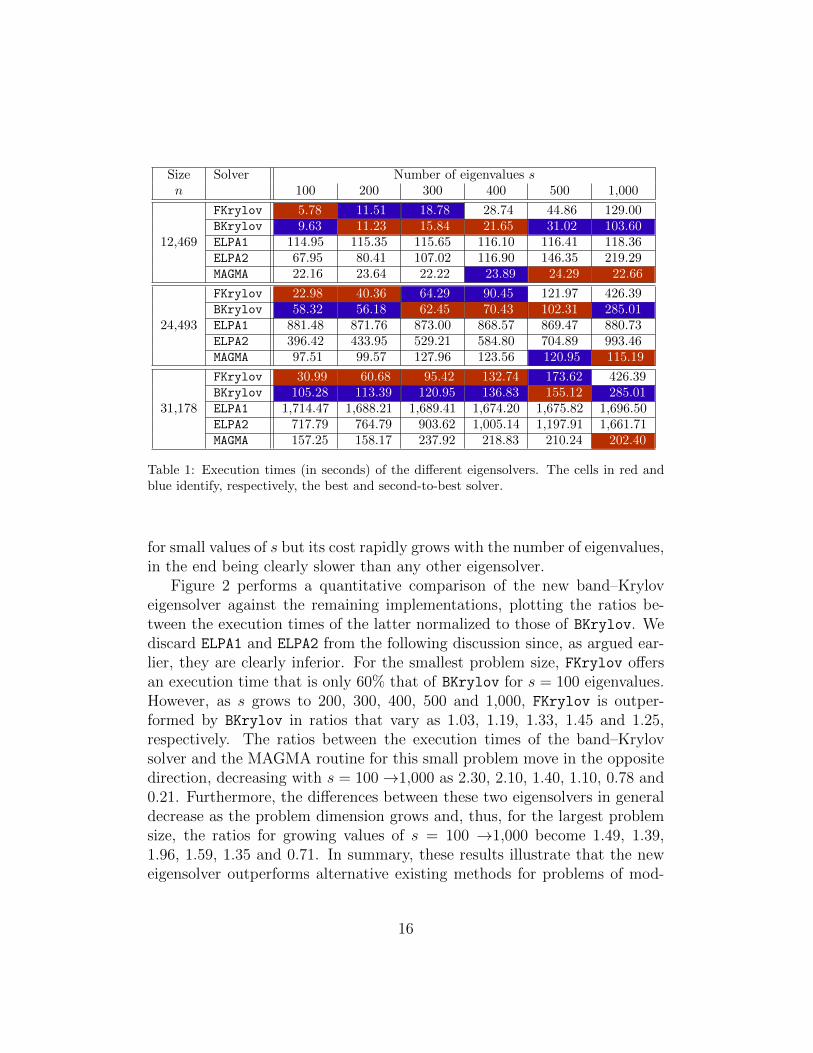
Table 1 reports the execution of the eigensolvers for all three instances ofthe macromolecule MT and required number of eigenvalues s. These resultsexpose that the band–Krylov eigensolver is the best or second-to-best optionfor all practical scenarios. In general, the fastest eigensolver is FKrylov

for small values of s, BKrylov for moderate s, and MAGMA for large s, withthe threshold values that define “small”, “moderate” and “large” dependingon the problem size n. ELPA1 exhibits execution times which are mostlyindependent of the number of required eigenvalues. ELPA2 outperforms ELPA1

1http://elpa.rzg.mpg.de/.2http://icl.cs.utk.edu/magma/.

15

Size Solver Number of eigenvalues sn 100 200 300 400 500 1,000

12,469

FKrylov 5.78 11.51 18.78 28.74 44.86 129.00BKrylov 9.63 11.23 15.84 21.65 31.02 103.60ELPA1 114.95 115.35 115.65 116.10 116.41 118.36ELPA2 67.95 80.41 107.02 116.90 146.35 219.29MAGMA 22.16 23.64 22.22 23.89 24.29 22.66

24,493

FKrylov 22.98 40.36 64.29 90.45 121.97 426.39BKrylov 58.32 56.18 62.45 70.43 102.31 285.01ELPA1 881.48 871.76 873.00 868.57 869.47 880.73ELPA2 396.42 433.95 529.21 584.80 704.89 993.46MAGMA 97.51 99.57 127.96 123.56 120.95 115.19

31,178

FKrylov 30.99 60.68 95.42 132.74 173.62 426.39BKrylov 105.28 113.39 120.95 136.83 155.12 285.01ELPA1 1,714.47 1,688.21 1,689.41 1,674.20 1,675.82 1,696.50ELPA2 717.79 764.79 903.62 1,005.14 1,197.91 1,661.71MAGMA 157.25 158.17 237.92 218.83 210.24 202.40

Table 1: Execution times (in seconds) of the different eigensolvers. The cells in red andblue identify, respectively, the best and second-to-best solver.

for small values of s but its cost rapidly grows with the number of eigenvalues,in the end being clearly slower than any other eigensolver.

Figure 2 performs a quantitative comparison of the new band–Kryloveigensolver against the remaining implementations, plotting the ratios be-tween the execution times of the latter normalized to those of BKrylov. Wediscard ELPA1 and ELPA2 from the following discussion since, as argued ear-lier, they are clearly inferior. For the smallest problem size, FKrylov offersan execution time that is only 60% that of BKrylov for s = 100 eigenvalues.However, as s grows to 200, 300, 400, 500 and 1,000, FKrylov is outper-formed by BKrylov in ratios that vary as 1.03, 1.19, 1.33, 1.45 and 1.25,respectively. The ratios between the execution times of the band–Krylovsolver and the MAGMA routine for this small problem move in the oppositedirection, decreasing with s = 100→1,000 as 2.30, 2.10, 1.40, 1.10, 0.78 and0.21. Furthermore, the differences between these two eigensolvers in generaldecrease as the problem dimension grows and, thus, for the largest problemsize, the ratios for growing values of s = 100 →1,000 become 1.49, 1.39,1.96, 1.59, 1.35 and 0.71. In summary, these results illustrate that the neweigensolver outperforms alternative existing methods for problems of mod-

16

Number of eigenvalues100 200 300 400 500 1000

Ra

tio

w.r

.t.

BK

rylo

v

0

0.5

1

1.5

2

2.5

3n=12,469

FKrylovBKrylovMAGMA

Number of eigenvalues100 200 300 400 500 1000

Ra

tio

w.r

.t.

BK

rylo

v

0

0.5

1

1.5

2

2.5n=24,943

FKrylovBKrylovMAGMA

Number of eigenvalues100 200 300 400 500 1000

Ra

tio

w.r

.t.

BK

rylo

v

0

0.5

1

1.5

2n=31,178

FKrylovBKrylovMAGMA

Figure 2: Experimental comparison of the different eigensolvers. Performance ratios corre-spond to execution times normalized with respect to that of the band–Krylov eigensolver.

erate dimension when the number of eigenpairs to be computed is small tomoderate.

6. Concluding Remarks

We have presented a mixed eigensolver that combines the high-performancereduction to band form typical of direct multi-stage methods with the low-cost iteration of Krylov subspace methods. By appropriately choosing thebandwidth of the intermediate matrix that represents the problem, our hy-brid band–Krylov eigensolver can thus shift part of its cost towards (awayfrom) the initial band reduction and away from (towards) the Krylov itera-tion. The balance between these two stages is achieved taking into accountthe problem dimensions, convergence rate of the problem, target architecture,and efficiency of the underlying method. The solver is completed with a tai-

17

lored symmetric band matrix-vector product that off-loads this operation tothe GPU, resulting in a significant acceleration of the Krylov iteration.

The results using a server equipped with recent multi-core Intel Xeon tech-nology and an NVIDIA Tesla “Kepler” show the performance superiority ofthe new band–Krylov eigensolver for the simulation of macromolecules with afew thousands degrees of freedom when the required number of eigenpairs issmall to moderate. As an additional advantage, the new band–Krylov solvercan handle larger problems on the GPU, as the initial reduction to bandform can be performed out-of-core from the perspective of the accelerator,while the subsequent Krylov iteration proceeds in-core on a band matrix ofreduced size.

Acknowledgements

This work was supported by the CICYT projects TIN2011-23283 andTIN2014-53495-R of the MINECO and FEDER, and project P1-1B2013-20of the Fundacio Caixa Castello-Bancaixa and UJI.

References

[1] I. Bahar, A. J. Rader, Coarse-grained normal mode analysis in structuralbiology, Curr. Opin. Struct. Biology 15 (5) (2005) 586–92.

[2] V. Tozzini, Minimalist models for proteins: a comparative analysis, Q.Rev. Biophys. 43 (3) (2010) 333–71.

[3] C. N. Cavasotto, J. A. Kovacs, R. A. Abagyan, Representing recep-tor flexibility in ligand docking through relevant normal modes, J. Am.Chem. Soc. 127 (26) (2005) 9632–40.

[4] P. Chacon, F. Tama, W. Wriggers, Mega-dalton biomolecular motioncaptured from electron microscopy reconstructions, J. Mol. Biol. 326 (2)(2003) 485–92.

[5] M. Delarue, P. Dumas, On the use of low-frequency normal modes to en-force collective movements in refining macromolecular structural models,Proc. Natl. Acad. Sci. USA 101 (18) (2004) 6957–62.

18

[6] J. Franklin, P. Koehl, S. Doniach, M. Delarue, Minactionpath: max-imum likelihood trajectory for large-scale structural transitions in acoarse-grained locally harmonic energy landscape, Nucleic Acids Res.35 (Web Server issue).

[7] K. Hinsen, E. Beaumont, B. Fournier, J. J. Lacapere, From electronmicroscopy maps to atomic structures using normal mode-based fitting,Methods Mol. Biol. 654 (2010) 237–58.

[8] A. May, M. Zacharias, Energy minimization in low-frequency normalmodes to efficiently allow for global flexibility during systematic protein-protein docking, Proteins 70 (3) (2008) 794–809.

[9] J. R. Lopez-Blanco, J. I. Garzon, P. Chacon, iMod: multipurpose normalmode analysis in internal coordinates, Bioinformatics 27 (20) (2011)2843–50.

[10] J. Aliaga, P. Bientinesi, D. Davidovic, E. D. Napoli, F. Igual, E. S.Quintana-Ortı, Solving dense generalized eigenproblems on multi-threaded architectures, Appl. Math. & Comp. 218 (22) (2012) 11279–11289.

[11] J. R. Lopez-Blanco, R. Reyes, J. I. Aliaga, R. M. Badia, P. Chacon,E. S. Quintana, Exploring large macromolecular functional motions onclusters of multicore processors, J. Comp. Phys. 246 (2013) 275–288.

[12] W. G. Krebs, V. Alexandrov, C. A. Wilson, N. Echols, H. Yu, M. Ger-stein, Normal mode analysis of macromolecular motions in a databaseframework: developing mode concentration as a useful classifying statis-tic, Proteins 48 (4) (2002) 682–95.

[13] L. Yang, G. Song, R. L. Jernigan, How well can we understand large-scale protein motions using normal modes of elastic network models?,Biophys. J. 93 (3) (2007) 920–9.

[14] L. Orellana, M. Rueda, C. Ferrer-Costa, J. R. Lopez-Blanco, P. Chacon,M. Orozco, Approaching elastic network models to molecular dynamicsflexibility, J. Chem. Theory Comput. 6 (9) (2010) 2910–2923.

19

[15] M. Rueda, P. Chacon, M. Orozco, Thorough validation of protein normalmode analysis: a comparative study with essential dynamics, Structure15 (5) (2007) 565–75.

[16] A. Ahmed, S. Villinger, H. Gohlke, Large-scale comparison of proteinessential dynamics from molecular dynamics simulations and coarse-grained normal mode analyses, Proteins 78 (16) (2010) 3341–52.

[17] G. H. Golub, C. F. V. Loan, Matrix Computations, 3rd Edition, TheJohns Hopkins University Press, Baltimore, 1996.

[18] E. Anderson, Z. Bai, J. Demmel, J. E. Dongarra, J. DuCroz, A. Green-baum, S. Hammarling, A. E. McKenney, S. Ostrouchov, D. Sorensen,LAPACK Users’ Guide, SIAM, Philadelphia, 1992.

[19] MAGMA project home page, http://icl.cs.utk.edu/magma/.

[20] C. H. Bischof, B. Lang, X. Sun, Algorithm 807: The SBR Toolbox—software for successive band reduction, ACM Trans. Math. Soft. 26 (4)(2000) 602–616.URL http://doi.acm.org/10.1145/365723.365736

[21] PLASMA project home page, http://icl.cs.utk.edu/plasma/.

[22] D. Davidovic, E. S. Quintana-Ortı, Applying OOC techniques in thereduction to condensed form for very large symmetric eigenproblems onGPUs, in: 20th Euro. Conf. PDP 2012, 2012, pp. 442–449.

[23] T. Auckenthaler, V. Blum, H.-J. Bungartz, T. Huckle, R. Johanni,L. Krmer, B. Lang, H. Lederer, P. Willems, Parallel solution of partialsymmetric eigenvalue problems from electronic structure calculations,Parallel Computing 37 (12) (2011) 783 – 794.

[24] A. Haidar, R. Solca, M. Gates, S. Tomov, T. Schulthess, J. Dongarra,Leading edge hybrid multi-gpu algorithms for generalized eigenprob-lems in electronic structure calculations, in: J. M. Kunkel, T. Ludwig,H. Meuer (Eds.), Supercomputing, Vol. 7905 of Lecture Notes in Com-puter Science, Springer Berlin Heidelberg, 2013, pp. 67–80.

20

[25] P. Bientinesi, F. D. Igual, D. Kressner, M. Petschow, E. S. Quintana-Ortı, Condensed forms for the symmetric eigenvalue problem on multi-threaded architectures, Concurrency and Computation: Practice andExperience 23 (7) (2011) 694–707.

[26] ARPACK project home page, http://www.caam.rice.edu/software/ARPACK/.

[27] M. A. Deriu, M. Soncini, M. Orsi, M. Patel, J. W. Essex, F. M. Mon-tevecchi, A. Redaelli, Anisotropic elastic network modeling of entire mi-crotubules, Biophysical Journal 99 (2011) 2190–2199.

[28] J. R. Lopez-Blanco, J. I. Aliaga, E. S. Quintana-Ortı, P. Chacon,iMODS: internal coordinates normal mode analysis server, Nucleic AcidsResearch 42 (2014) W271–W276.

[29] J. R. Lopez-Blanco, P. Chacon, iMODFIT: Efficient and robust flexiblefitting based on vibrational analysis in internal coordinates, Journal ofStructural Biology 184 (2013) 261–270.

21