afit/gtm/lal/96s-6 · afit/gtm/lal/96s-6 a study of defense ... advantages of the eoq ......

AFIT/GTM/LAL/96S-6

A STUDY OF DEFENSE LOGISTICS AGENCY INVENTORYCLASSIFICATIONS: APPLICATION OF INVENTORY CONTROL

METHODS TO REDUCE TOTAL VARIABLE COST ANDSTOCKAGE LEVELS

THESIS

Wayne C. Goulet Michael L. Rollman Captain, USAF 1st Lieutenant, USAF

AFIT/GTM/LAL/96S-6

Approved for public release; distribution unlimited

The views expressed in this thesis are those of the authorsand do not reflect the official policy or position of the

Department of Defense or the U.S. Government.

AFIT/GTM/LAL/96S-6

A STUDY OF DEFENSE LOGISTICS AGENCY INVENTORY

CLASSIFICATIONS: APPLICATION OF INVENTORY CONTROL

METHODS TO REDUCE TOTAL VARIABLE COST AND

STOCKAGE LEVELS

THESIS

Presented to the Faculty of the Graduate School of Logistics

and Acquisition Management of the Air Force Institute of Technology

Air University

Air Education and Training Command

In Partial Fulfillment of the

Requirements for the Degree of

Master of Science in Logistics Management

Wayne C. Goulet, B.S. Michael L. Rollman, B.S.

Captain, USAF 1st Lieutenant, USAF

September 1996

Approved for public release; distribution unlimited

ii

Acknowledgments

We wish to express our heartfelt thanks to our thesis co-advisors, Dr. Rajesh

Srivastava and Dr. V. Daniel R. Guide, Jr. for their support and insight during this

research effort. Additionally, we would like to thank Major Mark Kraus for his

assistance with the simulation models, and our classmates Major J.C. Penny and Captain

Tim Pettit for their input.

A special thanks to Mr. Jim Wager and Mr. Robert Bilikam, operations analysts,

and Ms. Kathy Fisher, stock control analyst at Defense Supply Center-Columbus for their

assistance in data collection and answering the many questions generated by this study.

Finally, but most importantly, we’d like to thank our wives, Bethsabet and Suk

Cha, for bearing more than their share of this burden for these last 16 months.

Wayne C. Goulet Mike L. Rollman

iii

Table of Contents

Page

Acknowledgments........................................................................................................... ii

List of Figures............................................................................................................... vii

List of Tables ...............................................................................................................viii

Abstract.......................................................................................................................... x

I. Background and Problem Presentation......................................................................... 1

Introduction ........................................................................................................... 1

Background........................................................................................................... 2

Inventory Classification and Categorization ........................................................... 4

Problem Statement................................................................................................. 8

Investigative Questions.......................................................................................... 8

Research Approach................................................................................................ 8

Methodology.......................................................................................................... 9

Scope and Limitations.......................................................................................... 10

Organization of Thesis......................................................................................... 10

II. Literature Review..................................................................................................... 12

Introduction ......................................................................................................... 12

What is inventory?............................................................................................... 12

Historical Views of Inventory .............................................................................. 14

Continuous Review Inventory Systems ................................................................ 15

Order-Point, Order-Quantity (s, Q) System........................................................... 16

Demand Patterns.................................................................................................. 17

Inventory Costs.................................................................................................... 18

Related Studies.................................................................................................... 19

Summary ............................................................................................................. 21

III. Continuous Review Inventory Models..................................................................... 23

Introduction ......................................................................................................... 23

iv

Page

EOQ Model ......................................................................................................... 23

Advantages of the EOQ ....................................................................................... 26

Disadvantages of the EOQ ................................................................................... 26

DLA’s EOQ Model.............................................................................................. 27

Periodic Order Quantity....................................................................................... 29

Silver-Meal Heuristic........................................................................................... 29

Advantages of the Silver-Meal Heuristic.............................................................. 30

Disadvantages of the Silver-Meal Heuristic.......................................................... 31

Conclusion........................................................................................................... 31

IV. Methodology........................................................................................................... 32

Introduction ......................................................................................................... 32

The Scientific Method.......................................................................................... 32

Steps of the Scientific Method ............................................................................. 33

Selection and Definition of the Problem............................................................... 34

Experimentation................................................................................................... 35

Experimental Design............................................................................................ 35

Why Simulation? ................................................................................................. 36

Simulation Language ........................................................................................... 37

Simulation Models............................................................................................... 37

Relevant Variables............................................................................................... 38

Verification and Validation.................................................................................. 38

Input Data............................................................................................................ 39

Steady State ......................................................................................................... 39

Number of Output Data Collection Runs.............................................................. 40

Inferences About the Difference Between Two Population Means ....................... 41

Statement of Hypotheses Conclusions.................................................................. 42

Summary ............................................................................................................. 42

V. Data Analysis .......................................................................................................... 44

Introduction ......................................................................................................... 44

v

Page

Analysis of Input Data ......................................................................................... 44

Model Starting Conditions ................................................................................... 46

Model Validation and Verification....................................................................... 47

Number of Output Data Collection Runs.............................................................. 47

Analysis of Output Data....................................................................................... 51

Average On-Hand Inventory................................................................................ 51

Total Variable Costs ............................................................................................ 57

Summary ............................................................................................................. 63

VI. Conclusions, Implications and Recommendations ................................................... 65

Introduction ......................................................................................................... 65

Problem Statement and Investigative Questions ................................................... 65

Investigative Questions........................................................................................ 65

Problem Statement............................................................................................... 69

Recommendations for Future Research ................................................................ 69

Summary ............................................................................................................. 70

Appendix A. Sample of Data from DSCC........................................................... 71

Appendix B. Sample Input Distribution Analysis................................................ 72

Appendix C. Sample Proposed Empirical Arrays ................................................ 73

Appendix D. Starting Conditions for Each SMCC ............................................... 74

Appendix E. Input Arrays ................................................................................... 75

Appendix F. DLA EOQ SLAM Model Variable Definitions............................... 76

Appendix G. Silver-Meal SLAM Model Variable Definitions............................. 77

Appendix H. Periodic Order Quantity SLAM Model Variable Definitions.......... 78

Appendix I. DLA EOQ SLAM Model ................................................................ 79

Appendix J: DLA EOQ SLAM Subroutine Fortran Code.................................... 85

Appendix K: Silver-Meal SLAM Model ............................................................. 87

Appendix L: Silver-Meal SLAM Subroutine Fortran Code ................................. 92

Appendix M. Periodic Order Quantity SLAM Model.......................................... 95

Appendix N. Periodic Order Quantity FORTRAN Subroutine .......................... 100

Appendix O. Verification of the Silver-Meal Model ......................................... 102

vi

Page

Appendix P. Verification of the Periodic Order Quantity .................................. 105

Appendix Q. Verification of the DLA Economic Order Quantity Model........... 108

References......................................................................................................... 111

Goulet Vita ........................................................................................................ 114

Rollman Vita ..................................................................................................... 115

vii

List of Figures

Figure Page

2-1. ORDER-POINT, ORDER-QUANTITY (S, Q) SYSTEM.................................................................16

3-1. COST FUNCTIONS OF THE EOQ................................................................................................25

viii

List of Tables

Table Page

1-1. COMMODITY ASSIGNMENT BY DLA CENTER.........................................................................3

1-2. ABC INVENTORY CLASSIFICATIONS........................................................................................5

1-3. WEAPON SYSTEM GROUP (CRITICALITY) CODE (WSGC)......................................................6

1-4. WEAPON SYSTEM ESSENTIALITY CODE (WSEC)....................................................................6

1-5. WEAPON SYSTEM INDICATOR CODE (WSIC) MATRIX...........................................................7

1-6. BAND/SMCC MATRIX...................................................................................................................7

2-1. INVENTORY FUNCTIONAL FACTORS......................................................................................13

2-2. REASONS FOR HOLDING INVENTORY....................................................................................14

3-1. EOQ ASSUMPTIONS....................................................................................................................24

3-2. DLA FORECASTING METHODS.................................................................................................27

4-1. CHARACTERISTICS OF SCIENTIFIC RESEARCH....................................................................33

4-2. FIVE STEPS OF THE SCIENTIFIC METHOD..............................................................................33

5-1. ADJUSTED NSN COUNT.............................................................................................................45

5-2. MEAN TBO THEORETICAL DISTRIBUTION EVALUATION BY SMCC.................................46

5-3. MEAN QPD THEORETICAL DISTRIBUTION EVALUATION BY SMCC.................................46

5-4. SIMULATION RUNS TEST - SMCC 0 AVERAGE ON-HAND INVENTORY.............................48



5-7. SIMULATION RUNS TEST - SMCC 0 TOTAL VARIABLE COST.............................................49



5-11. AVERAGE ON-HAND INVENTORY LEVELS..........................................................................51

5-12. SMCC 0 DLA EOQ AND SILVER-MEAL PAIRED DIFFERENCE TEST..................................52

5-13. SMCC 0 DLA EOQ AND POQ PAIRED DIFFERENCE TEST...................................................52

ix

Table Page

5-14. SMCC 0 SILVER-MEAL AND POQ PAIRED DIFFERENCE TEST...........................................53







5-21. TOTAL VARIABLE COST VALUES..........................................................................................58










6-1. SUMMARY OF AVERAGE ON-HAND INVENTORY RESULTS...............................................66

6-2. SUMMARY OF TOTAL VARIABLE COST RESULTS................................................................66

x

AFIT/GTM/LAL/96S-6

Abstract

This thesis analyzes the financial impact of applying a single inventory

requirements model to three separate classes of inventory at the Defense Logistics

Agency’s (DLA) Defense Supply Center-Columbus (DSCC) commodity management

facility. DLA’s blanket application of its variation of the Economic Order Quantity

(EOQ) requirements model may not be appropriate for all levels of demand, possibly

suboptimizing DLA’s desire to minimize inventory costs while still providing an

appropriate level of customer service. Simulation analyses of the DLA EOQ

requirements model, the Silver-Meal heuristic, and Periodic Order Quantity models were

conducted to examine which dynamic lot-sizing model is more effective in minimizing

inventory costs and levels for different levels of item demand. The Periodic Order

Quantity model provided lower inventory levels and total variable costs than the DLA

EOQ and the Silver-Meal models for the medium demand category. The DLA EOQ

requirements model was found to provide lower inventory levels and total variable costs

than either the POQ or the Silver-Meal models in the low and high demand categories.

1

A Study of Defense Logistics Agency Inventory Classifications:

Application of Inventory Control Methods to Reduce

Total Variable Cost and Stockage Levels

I. Background and Problem Presentation

Introduction

In recent years there has been increasing pressure on the federal government to

reduce its size and hence, its expenditures of tax revenues. The government has

responded in a variety of ways, including reorganizations, consolidations, downsizings,

and reductions in all facets of the public sector. As one of the larger recipients of public

moneys, the Department of Defense (DoD) has not escaped the axe wielded by

government budget cutters. DoD senior leaders have had to make tough operational

choices to balance the required level of mission readiness with the need for a smaller,

more economical, yet effective military. The DoD’s logistics system has emerged as a

prime target for reductions and savings. Logistics managers throughout the DoD have

been challenged to reduce inventories to save money.

The Defense Logistics Agency (DLA) is the largest provider of supplies in the

DoD inventory system, managing over 3.8 million items valued at over $11 billion for

the military services (DLA, 1996: 1). To improve management and visibility of its

inventory, each of DLA’s six commodity centers has established local procedures to

facilitate the grouping and control of items assigned to their particular center. As an

example, the Defense Supply Center - Columbus, Ohio (DSCC) has established

2

classifications based on the combination of: 1) an item’s annual usage in dollars, and 2)

the mission criticality of the part. Although each supply center uses a different

classification method to group items, each DLA center uses the same economic order

quantity (EOQ) inventory requirements model to determine reorder quantities for all

items, regardless of classification. The “blanket” application of a single requirements

model may not be appropriate for all classes, possibly suboptimizing DLA’s desire to

minimize inventory costs while still providing an appropriate level of customer service.

This study will analyze the financial impact of applying a single inventory requirements

model to separate classes of inventory at DLA’s Defense Supply Center - Columbus

commodity management facility.

Background

In 1961, after approximately 19 attempts to establish a civilian run supply agency

to provide logistics support to the military departments, Secretary of Defense Robert

McNamara announced the establishment of the Defense Supply Agency (DSA). The

goal of this organization was to consolidate the 20 different numbering systems and 8

different item classifications that existed throughout the services at that time. On 1

October 1961, Lt. General Andrew T. McNamara was appointed as DSA’s first director.

General McNamara emphasized that the success of DSA would depend on the

decentralization of the organization, delegation of authority to field commanders,

procurement competition, simplification of the supply system, and standardization

(Robinson, 1993: 3).

In 1977, DSA became the Defense Logistics Agency (DLA). DLA is

headquartered in Alexandria, Virginia, and its mission is:

...to function as an integral element of the DoD logistics system and to provideeffective and efficient worldwide logistics support to DoD components as well asto Federal Agencies, foreign governments, or international organizations as

3

assigned in peace and war. (Its) vision ideally is to continually improve thecombat readiness of America’s fighting forces by providing soldiers, sailors,airmen, and marines the best value and services when and where needed.(Robinson, 1993: 6)

DLA is responsible for the management of over 3.8 million consumable items in

support of the military services. The commodities managed by DLA include fuel, food,

clothing, and medical supplies, as well as general supply items. In total, DLA is

responsible for 86 percent of the consumable items required by the Air Force, Navy,

Army, and Marine Corps (DLA Pamphlet, 1992: 2).

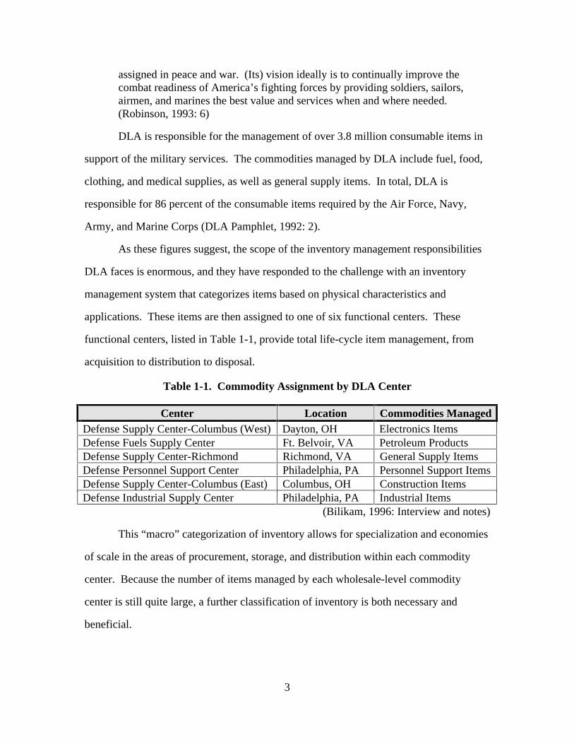
As these figures suggest, the scope of the inventory management responsibilities

DLA faces is enormous, and they have responded to the challenge with an inventory

management system that categorizes items based on physical characteristics and

applications. These items are then assigned to one of six functional centers. These

functional centers, listed in Table 1-1, provide total life-cycle item management, from

acquisition to distribution to disposal.

Table 1-1. Commodity Assignment by DLA Center

Center Location Commodities ManagedDefense Supply Center-Columbus (West) Dayton, OH Electronics ItemsDefense Fuels Supply Center Ft. Belvoir, VA Petroleum ProductsDefense Supply Center-Richmond Richmond, VA General Supply ItemsDefense Personnel Support Center Philadelphia, PA Personnel Support ItemsDefense Supply Center-Columbus (East) Columbus, OH Construction ItemsDefense Industrial Supply Center Philadelphia, PA Industrial Items

(Bilikam, 1996: Interview and notes)

This “macro” categorization of inventory allows for specialization and economies

of scale in the areas of procurement, storage, and distribution within each commodity

center. Because the number of items managed by each wholesale-level commodity

center is still quite large, a further classification of inventory is both necessary and

beneficial.

4

Inventory Classification and Categorization

Inventory can be classified into groups to allow for an appropriate level of control

over items in the groups. Detailed, or increased, inventory control of an item is costly

and it is usually uneconomical to apply detailed control on all items in an inventory

(Tersine & Campbell, 1977: 162). Some items require increased control or visibility due

to characteristics such as usage, value, or criticality.

Critical items are defined as those assets that are crucial to the operation of the

firm. The lack of these items when required could result in the shutdown of production

lines or the permanent loss of future sales due to the deterioration of customer goodwill.

From a military standpoint, critical items are necessary to maintain weapons systems (i.e.

aircraft, tanks, ships, etc.) in a fully operational status.

One classification scheme that separates inventory into distinct classes based on

all three of the above characteristics is the ABC classification method. The ABC method

is based on a concept attributed to Vilfredo Pareto known as the “Pareto Principle.” In

essence, the Pareto Principle states that many situations are dominated by a relatively

vital few elements (Magad & Amos, 1989: 123). The ABC classification scheme is an

inventory application of the Pareto Principle and states that whenever inventory is held, a

large percentage of the dollar investment in stock is concentrated on relatively few items

(Ammer, 1980: 288). The figures vary from text to text, but it is generally

acknowledged that between 10 and 20 percent of the items held in inventory will account

for 80 to 90 percent of the annual usage dollar value of the inventory. These 10-20

percent high value items are categorized as class “A." Management decides the

appropriate placement of the remainder of the items, either in categories “B” or “C”

depending on their value and operational criticality. Table 1-2 lists the three categories

of the ABC classification method:

5

Table 1-2. ABC Inventory Classifications

Classification DescriptionA Items with high demand/large unit valueB Items with low demand or small unit valueC Items with low demand and small unit value

By segregating inventory in this fashion, firms can focus their attention on the

small group of class “A” items that account for the highest annual dollar volume (number

of items demanded multiplied by unit value) and which absorb most of the inventory

budget. These items are given careful consideration when forecasting, planning, and

controlling inventories because they offer the potential for greater financial benefits if

managed properly. Small or no savings can be expected from optimizing the control of

“B” and “C” items (Petrovic, Senborn & Vujosevic, 1986: 12-13). Because of the

extraordinary number of items stocked and its desire to minimize inventory control costs,

DLA uses the ABC inventory classification system to effectively manage inventories at

its commodity centers

Each DLA center commander is given authority to apply a customized version of

the ABC inventory classification method most appropriate for the types of items

managed by the center under their command. As mentioned in the introduction, this

study will evaluate the Defense Supply Center-Columbus (DSCC) as the representative

DLA commodity center. The DSCC commander has chosen a variation of the ABC

method that classifies items based on a combination of the following item characteristics:

1. Annual Demand Frequency (ADF). The number of orders or requisitions

received by DSCC in one year for a specific inventory item.

2. Annual Demand Value (ADV). The unit price of an item multiplied by the

total quantity demanded in one year.

3. Weapon System Group (Criticality) Code (WSGC). The military services

provide this code to DLA for each National Stock Number (NSN) based upon

6

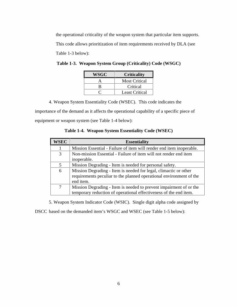
the operational criticality of the weapon system that particular item supports.

This code allows prioritization of item requirements received by DLA (see

Table 1-3 below):

Table 1-3. Weapon System Group (Criticality) Code (WSGC)

WSGC CriticalityA Most CriticalB CriticalC Least Critical

4. Weapon System Essentiality Code (WSEC). This code indicates the

importance of the demand as it affects the operational capability of a specific piece of

equipment or weapon system (see Table 1-4 below):

Table 1-4. Weapon System Essentiality Code (WSEC)

WSEC Essentiality1 Mission Essential - Failure of item will render end item inoperable.3 Non-mission Essential - Failure of item will not render end item

inoperable.5 Mission Degrading - Item is needed for personal safety.6 Mission Degrading - Item is needed for legal, climactic or other

requirements peculiar to the planned operational environment of theend item.

7 Mission Degrading - Item is needed to prevent impairment of or thetemporary reduction of operational effectiveness of the end item.

5. Weapon System Indicator Code (WSIC). Single digit alpha code assigned by

DSCC based on the demanded item’s WSGC and WSEC (see Table 1-5 below):

7

Table 1-5. Weapon System Indicator Code (WSIC) Matrix

WSIC WSGC WSEC WSIC WSGC WSEC WSIC WSGC WSECF A 1 H A 6 K A 3 or blankL B 1 P B 6 S B 3 or blankT C 1 X C 6 Z C 3 or blankG A 5 J A 7 N N/A N/AM B 5 R B 7W C 5 Y C 7

Based upon the five classification criteria listed above, DLA prioritizes inventory

categories by assigning a single digit numeric code referred to as the Selective

Management Category Code (SMCC). After assignment of the SMCC, DSCC assigns a

Band code to each inventory item, representing its version of the ABC classification

method. The Band code is used by DSCC to assign priorities for individual item

control. The Band/SMCC matrix is presented in Table 1-6 as follows:

Table 1-6. Band/SMCC Matrix

BAND SMCC ADF ADV WSIC WSGC WSEC

A 1 150+ >$7000 F,G,H,J,K,L,M,P,R,S,T,W,X,Y,Z,N A,B,C 1,5,6,7,3, BlankA 2 150+ <=$7000 F,G,H,J,K,L,M,P,R,S,T,W,X,Y,Z,N A,B,C 1,5,6,7,3, BlankA 3 20-149 >$7000 F,G,H,J,K,L,M,P,R,S,T,W,X,Y,Z,N A,B,C 1,5,6,7,3, BlankA 4 20-149 <=$7000 F,G,H,J,K,L,M,P,R,S,T,W,X,Y,Z,N A,B,C 1,5,6,7,3, BlankA 5 4-19 >$7000 F,G,H,J,K A 1,5,6,7,3, Blank

L,T B,C 1A 6 4-19 <=$7000 F,G,H,J,K A 1,5,6,7,3, Blank

L,T B,C 1B 7 4-19 >$7000 M,P,R,S,W,X,Y,Z,N B,C 5,6,7,3, BlankB 8 4-19 <=$7000 M,P,R,S,W,X,Y,Z,N B,C 5,6,7,3, BlankC 9 0-3 >$7000 F,G,H,J,K,L,M,P,R,S,T,W,X,Y,Z,N A,B,C 1,5,6,7,3, BlankC 0 0-3 <=$7000 F,G,H,J,K,L,M,P,R,S,T,W,X,Y,Z,N A,B,C 1,5,6,7,3, Blank

The above inventory classification scheme gives DSCC managers visibility on the

critical few items that comprise the bulk of their inventory investment. This visibility

can be a vital tool when procurement decisions must be made, decisions that attempt to

maximize the use of available capital resources and satisfy mission requirements, while

minimizing the costs associated with ordering and holding inventory.

8

Problem Statement

DSCC may be sub-optimizing by using a single inventory requirements model to

determine order quantities for the different classes of inventory it manages. The research

question that will be addressed is:

Do different dynamic lot sizing models, when applied to the existing DSCC

classification structure, provide lower total variable costs and inventory

levels than the DLA EOQ requirements model?

Investigative Questions

The following investigative questions will be addressed to provide relevant

answers to the research question:

1. What are the results, in terms of costs and inventory levels, of applying the

DLA EOQ requirements model, the Silver-Meal Heuristic, and the Periodic

Order Quantity model to low, medium, and high demand items?

2. Which inventory model, the DLA EOQ requirements model, the Silver-Meal

Heuristic, or the Periodic Order Quantity model is more effective in

minimizing inventory costs and levels for low, medium, and high demand

items?

These questions will provide answers as to the effectiveness of the DLA

inventory requirements model, as compared to two other inventory models, the Silver-

Meal heuristic and the Periodic Order Quantity model.

Research Approach

The specific research steps that will be accomplished are:

9

1. Gather and adjust data from the Defense Supply Center-Columbus (DSCC) to

provide a database to evaluate the effects of different inventory models on

different classifications of inventory at DSCC.

2. Perform simulations of order-point, order-quantity (s, Q) consumable

inventory models, the DLA EOQ requirements model, the Silver-Meal

heuristic, and the Periodic Order Quantity model on different SMCC

classifications of inventory to determine the impact the different models have

on total variable costs and computed inventory levels.

3. Statistically determine if differences in the resulting cost and inventory

figures from the simulations are significant.

4. Determine which model is most effective at minimizing DSCC’s total

variable costs and inventory levels for each type of demand; low, medium,

and high.

Methodology

The tool used to accomplish the research objectives and answer the research

question will be simulation. Simulation is preferable to analytic models because of the

flexibility it offers when analyzing complex inventory problems. Simulation models for

the DLA EOQ requirements model, the Silver-Meal heuristic, and the Periodic Order

Quantity will be developed to measure on-hand inventory and total variable costs

realized by the respective ordering schemes. Real-world data from each of DSCC’s

inventory classes will be statistically analyzed to provide accurate order frequency and

order quantity input to the models. Simulation output from the three models will then be

statistically compared to determine which inventory model is most effective at

minimizing costs and inventory levels for different SMCC classifications.

10

Scope and Limitations

1. Due to time and budgetary limitations, research will be limited to items

managed by DSCC. DLA must determine if results are applicable to their

entire inventory management system.

2. DLA’s inventory forecasting model will be not be evaluated in this study.

The forecasting method used will approximate the Naive Forecast 1 technique

where actual demand from the past period serves as the forecasted demand for

the present period. In-depth evaluation of the forecasting method is beyond

the scope of this research.

3. Three of DLA’s ten SMCC classifications will be simulated. These three

classifications will represent high, medium, and low demand items as

determined by DSCC’s Band/SMCC matrix (see Table 1-6). Specifically,

high demand items are those with 150 or more demands per year, medium

demand items have between 4 and 149 demands annually, and low demand

items experience fewer than 4 annual demands.

4. Analysis of the inventory ordering schemes will be limited to quantifiable

costs incurred in the operation of an inventory system. Factors such as

customer service levels and issue effectiveness are beyond the scope of this

study.

Organization of Thesis

Chapter I has provided an introduction to the issues surrounding DLA’s inventory

management system. Background information has been provided to assist the reader in

understanding the potential for total variable cost and inventory level reductions through

application of a different inventory model to the different classes of inventory managed

by DSCC. Chapter II will provide a review of literature relevant to the problem.

11

Chapter III will describe, in detail, the inventory models selected for evaluation. Chapter

IV describes the methodological approach used to assist in evaluating the effectiveness of

the different inventory models. This chapter will further discuss the concept and

application of simulation as a research tool. Data obtained from model simulations will

be analyzed and discussed in Chapter V. This will include the type of data obtained and

the analytical methods used to test the proposed hypotheses. Chapter VI will contain the

results of the analyses conducted in Chapter V. The investigative questions posed in

Chapter I will be addressed. The overall conclusion as to the effectiveness of applying

DLA’s requirements model to all classes of inventory held will be provided, and

additional areas of exploration for follow-on study will be suggested.

12

II. Literature Review

Introduction

This chapter will explore various concepts governing consumable item

management. Specifically, it will provide the framework for an understanding of the

importance of total variable costs and inventory levels as measures for evaluating the

effectiveness of inventory requirements models when applied to DLA’s inventory

classifications. First, this chapter will define inventory, explain why stocks are held, and

explore the evolution of contemporary views towards the accumulation of inventory.

Next, inventory costs will be discussed, followed by an examination of continuous

review inventory systems, with emphasis on the continuous review order-point, order-

quantity (s, Q) system currently used by DLA. Then, inventory demand patterns and

their impact on the calculation of reorder quantities will be presented. Finally, previous

research that has contributed to this study will be reviewed.

What is inventory?

“Very basically, inventory is required to satisfy demand” (Heilweil, 1986: 52).

Stephen F. Love defines inventory as “a quantity of goods or materials in the control of

an enterprise and held for a time in a relatively idle or unproductive state, awaiting its

intended use or sale” (1979: 3). In addition, Waters has further defined the difference

between stock and inventory. “Stock consists of all the goods and materials stored by an

organization. It is a supply of items which is kept for future use. Inventory is a list of

the items held in stock” (1992: 4). Stock acts as a buffer between supply and demand,

allowing operations to continue smoothly when the supply rate does not exactly match

13

the demand rate (Waters, 1992: 7). The major reason organizations hold stocks is to

ensure that a supply of an item will be available when it is needed (Barrett, 1969: 1).

Tersine states that “inventory exists because organizations cannot function

without it” (1982: 9). He further adds that inventory is held in a inactive or unproductive

state awaiting utilization for its intended purpose. Why inventory is held can be

explained by four functional factors: 1) time, 2) discontinuity, 3) uncertainty and, 4)

economy (Tersine, 1982: 6). These functional factors are summarized in Table 2-1 as

follows:

Table 2-1. Inventory Functional Factors

FunctionalFactor Why Inventory is Held Benefits of Holding InventoryTime For production and distribution

processes required beforedelivery to final consumers

- Decreases or eliminates consumer purchase waiting times- Firms can reduce lead times to satisfy demand

Discontinuity To treat retailing, distributing,warehousing, manufacturing,and purchasing as independentoperations

- Production is not geared directly to consumption- Consumption is not forced to adapt to production- Firms can schedule operations more efficiently

Uncertainty To adjust to unforeseen eventsthat alter organizational plans

- Protects the firm from unanticipated orunplanned circumstances

Economy To allow the firm to takeadvantage of cost reductionopportunities

- Enable the firm to purchase or produce items in economic quantities- Make bulk purchases with quantity discounts- Smooth production and manpower requirements for seasonal items

(Tersine, 1982: 9-10)

Complementing Tersine’s four functional factors of inventory are Waters’ reasons

for holding inventory as listed in Table 2-2:

14

Table 2-2. Reasons for Holding Inventory

- to act as a buffer between different operations- to allow for mismatches between supply and demand rates- to allow for demands which are larger than expected, or at unexpected times- to allow for deliveries which are delayed or too small- to avoid delays in passing products to customers- to take advantage of price discounts on large orders- to buy items when the price is low and expected to rise- to buy items which are going out of production or are difficult to find- to make full loads and reduce transport costs- to provide cover for emergencies- to maintain stable levels of operations

(Waters, 1992: 7)

Historical Views of Inventory

In the 1600s, inventory was perceived as a measure of wealth. Individuals would

collect and hold as much stock as possible because production and distribution of any

commodity (supply) was uncertain. However, at the turn of the 20th century, supplies

were no longer uncertain in the industrialized world. Consumers or manufacturers did

not have to buy goods as soon as they were available. Rather, they could wait until items

were needed before procurement (Waters, 1992: 23-24). In their book Decision Systems

for Inventory Management and Production Planning, Silver and Peterson point out that

inventories today represent large potential risk and are not seen as a measure of wealth.

They further state that corporate policy makers fear items held over and above actual

needs may become obsolete and will require disposal at considerable financial loss

(1985: 4). According to Tersine, there is an optimum level of inventory investment.

Having an excessive amount of inventory can impair corporate profits as much as having

too little inventory. “With inventories, too much can result in unnecessary holding costs,

and too little can result in lost sales or disrupted production. An organization must be

careful not to over-invest in inventory that ties up capital and may become obsolete, yet

it must take care not to run out of materials (thus idling people and equipment) or

15

products (thus losing sales and customers)” (Tersine, 1982: 10). To combat the

accumulation of excess inventories, firms now use “scientific inventory control”

methods. These methods include sophisticated models and mathematical analyses to set

optimal stock levels based on individual circumstances (Waters, 1992: 24). This study

will focus on scientific inventory control methods that compute reorder quantities using a

continuous review inventory system.

Continuous Review Inventory Systems

The DoD presently uses a continuous review inventory system to manage

wholesale and retail spares and repair parts (Perry, 1991: 1). Under this system, the

inventory or stock status is always known. The continuous review system immediately

updates an individual item’s inventory status at the time a transaction such as an issue,

receipt, or shipment is processed. In contrast, periodic review inventory systems

determine the inventory status of stocked items at fixed time intervals (Silver & Peterson,

1985: 255). Continuous review systems use the reorder point to signal the need for a

stock replenishment and the order quantity to determine how much to reorder. Order

quantities are usually based on procurement ordering cost and inventory holding cost

trade-offs. These trade-offs lead most firms to reorder a replenishment quantity, known

as the economic order quantity (EOQ), that balances ordering and holding costs to

minimize total variable costs (Perry, 1991: 1).

The greatest advantage of continuous review as compared to periodic review

inventory systems is the decreased amount of safety stock required under the continuous

review system. “This is because the period over which safety protection is required is

longer under periodic review (the stock level has the opportunity to drop appreciably

between review instants without any reordering action being possible in the interim)”

16

(Silver & Peterson, 1985: 255). The continuous review inventory system employed by

DLA is the order-point, order-quantity (s, Q) system (Perry, 1991: 1).

Order-Point, Order-Quantity (s, Q) System

Under the s, Q inventory system, a fixed order quantity (Q) (usually the EOQ) is

ordered after the inventory position has fallen to the reorder point or safety level (s) or

lower. This system is illustrated by a sawtooth diagram in Figure 2-1 as follows:

In v e n to ryP o s it io n

T im e

s

s + Q

E O Q E O Q E O Q

L e a dT im e

Figure 2-1. Order-Point, Order-Quantity (s, Q) System

(Plossl & Wight, 1967: 97)

In the s, Q system, the inventory position and not the quantity of stock in the

warehouse is used to initiate a replenishment order. The inventory position is used

because it includes the stock already on order but not yet received, eliminating the

possibility of placing a duplicate order before the first order is received. (Silver &

Peterson, 1985: 256). Figure 2-1 illustrates that at some point in time, the inventory

position of an item will fall to the reorder point s and trigger a replacement order for the

EOQ to raise the inventory level to Q. The inventory level will continue to fall during

17

the lead time (the time that elapses from the moment a replenishment order is placed

until the order is received into stock and is ready for use). Once the order is received, the

inventory position is increased by the EOQ, starting the cycle once again (Plossl &

Wight, 1967: 96).

Demand Patterns

Firms that sell goods experience varying demand patterns from their customers.

Determination of the type of demand an item experiences is crucial in the computation of

reorder quantities by inventory managers. Demand for goods held in inventory follows

either a deterministic (constant) or probabilistic (variable) demand pattern. The simplest

case of demand encountered by a company is deterministic, characterized by demand for

stocked items that is known in advance with certainty over a finite period. Inventory

systems based on deterministic demand are relatively uncomplicated to manage because

firms are not required to forecast for varying and uncertain inventory requirements.

However, it is uncommon for firms to experience deterministic demand for their products

in the real world. In reality, the typical demand pattern experienced by most firms in the

business environment is probabilistic, or random.

Probabilistic demand is often characterized by erratic demand patterns and

requires that inventory managers rely on sound forecasting techniques to aid in the

computation of order quantities which minimize inventory ordering and holding costs.

Lumpy demand, as defined by Peckham, is a special case of erratic demand often found

among low-volume, slow-moving items. These items show many periods with zero

demand, a low-average demand, and occasional demands which may be five or ten times

the average (Peckham, 1972: 48). In order to analytically calculate whether demand is

considered lumpy, Silver and Peterson have proposed the Variability Coefficient (VC)

measure, which is denoted as follows:

18

VC = Variance of demand per period

Square of average demand per period

(Silver & Peterson, 1985: 238)

If the value of VC is less than 0.2, the demand for the item is considered constant

and continuous (deterministic). If the VC is greater than or equal to 0.2, the demand

pattern is classified as lumpy. Lumpy demand for items makes it difficult for inventory

managers to calculate reorder quantities because customer demand cannot be predicted

with certainty. Too little inventory ordered may result in lost sales and customer

dissatisfaction while too much inventory ordered will unnecessarily increase inventory

costs.

Inventory Costs

Every firm that stores inventory incurs certain costs in the operation of an

inventory management system. Silver and Peterson list five relevant costs associated

with inventory. They are the unit value or unit variable cost, the cost of carrying items in

inventory, ordering costs, shortage costs, and system control costs (1985: 62-64).

The unit value or variable cost is also referred to as the purchase price plus freight

charges if the item is obtained from an external source. If the item is produced

internally, its value equals the unit production cost. Tersine states that “for purchased

items, it is the purchase price plus any freight cost. For manufactured items, the unit cost

includes direct labor, direct material, and factory overhead” (1982: 16).

Carrying or holding costs are the costs of holding one unit of an item in stock for

one unit of time. These costs include: 1) the opportunity cost of the money invested, 2)

the expenses incurred in running a warehouse, 3) the cost of special storage requirements,

4) deterioration of stocks, 5) obsolescence, and 6) insurance and taxes (Silver &

Peterson, 1985: 62). DSCC’s annual holding cost is 10 percent.

19

Ordering costs, according to Waters, consist of the costs incurred during order

placement and can include computer time, quality checks, correspondence, delivery,

telephone costs, expediting, use of equipment, and receiving (1992: 36). DSCC applies a

cost of $5.20 per order placed with its suppliers.

Shortage costs, also known as stockout costs, result when an item is not available

to fill a customer’s order. These costs are incurred as the company initiates an expedited

order to obtain the item as a backorder. The backorder can result in increased

transportation costs, handling costs, and special shipping and packaging costs. Shortage

costs can also include lost sales and loss of customer goodwill if the customer is not

willing to wait for the firm to receive the backorder. Lost sales result in reduced revenue

to the firm while a goodwill loss amounts to customers not returning to purchase

additional items in the future (Tersine, 1982: 17).

System control costs result from the firm’s implementation of specific inventory

control systems. Included in this category are the costs of data acquisition, data storage,

computation, and employee training (Silver & Peterson, 1985: 64).

The costs incurred through the management of an inventory system are a

necessary evil of doing business. However, to remain competitive, firms must ensure

they adopt a system that minimizes inventory costs while providing a management-

specified level of customer service.

Related Studies

Long and Engberson studied the effect of violations of the assumption of constant

demand on the DLA EOQ model. They collected data on 540 stock numbered items

managed by DLA and established a factorial design experiment with total variable cost,

average on hand inventory, and pre-replenishment inventory as response variables. The

response variables were designed to measure the effect of non-continuous or lumpy

20

demand on inventory costs. The factors established by the researchers were: 1) demand

pattern, 2) annual demand, and 3) lead time. Each factor contained three levels of

treatments.

Using the collected stock number data as input parameters, Long and Engberson

conducted numerous simulation runs of DLA’s EOQ formula. An analysis of the

simulation output revealed that the variances between treatment means were not equal

and independence was not achieved between simulation runs. As a result, Long and

Engberson were unable to use statistical tools to determine the effect of lumpy demand

on the EOQ model used by DLA and instead made practical observations on the output

data. The researchers concluded that lumpy demand caused average on hand inventory

to greatly fluctuate and required higher levels of safety stock. In addition, they

determined that lumpy demand varies the on-hand balances of stocked items, negatively

impacting customer support.

Berry and Tatge extended the research of Long and Engberson by evaluating the

overall suitability of the DLA EOQ model. Specifically, the purpose of their study was

to ascertain the overall impact of lumpy demand on DLA’s model and determine if a

better inventory model could be used in place of DLA’s current requirements model. To

quantify the effects of lumpy demand, Berry and Tatge identified two performance

measurements: total variable cost and average on-hand inventory. They postulated that if

total variable costs differed substantially under lumpy demand, this would demonstrate

that variable demand impacted DLA’s model greatly. Furthermore, if the average on-

hand inventory under lumpy demand differed significantly than under constant demand,

given that annual demand is the same under both conditions, then lumpy demand would

impact DLA’s model (Berry & Tatge, 1995: 3-3).

The researchers collected data on 525 national stock numbered items from DLA

and simulated DLA’s EOQ model under the three following demand conditions: 1)

21

constant and continuous, 2) normal, and 3) lumpy. Berry and Tatge also simulated the

Silver-Meal model under lumpy demand conditions to determine if this model handles

lumpy demand conditions better than DLA’s current requirements model. Their

simulation models incorporated the DLA quarterly forecasting model, a simple

exponential smoothing method which provided the demand projections required to run

the models.

Based upon their statistical analyses, Berry and Tatge determined that DLA’s

assumption of constant demand causes DLA to maintain higher inventory levels and that

lumpy demand causes DLA to incur greater total variable costs. They discovered that

average on-hand inventory and total variable costs increase from the constant and

continuous model to the normal model and from the normal model to the lumpy model.

Based upon these results, Berry and Tatge concluded that the DLA model “is not robust

enough to handle lumpy demand patterns” (Berry & Tatge, 1995: 5-2). In addition, they

discovered that the Silver-Meal model provided lower average inventory levels and lower

total variable costs than the current DLA EOQ model. This finding suggests that other

models exist that better handle lumpy demand patterns than the DLA EOQ model (Berry

& Tatge, 1995: 5-3).

Summary

This chapter has provided the necessary background to understand the

significance of this research. Topics covered included a definition of inventory and the

reasons why stocks are held. Continuous review inventory systems were described, with

an emphasis on the order-point, order-quantity (s, Q) system. Next, inventory costs were

discussed, followed by an examination of inventory demand patterns and their impact on

the calculation of reorder quantities. Finally, previous research that has contributed to

this study was reviewed. The next chapter will discuss DLA’s current EOQ requirements

22

model and two models that can be used in lieu of the EOQ, the Silver-Meal heuristic and

the Periodic Order Quantity model.

23

III. Continuous Review Inventory Models

Introduction

This chapter will explore the Economic Order Quantity (EOQ), the Periodic

Order Quantity (POQ), and the Silver-Meal heuristic. The basic arithmetic equations of

the three models will be presented followed by a discussion of the demand conditions

that favor the application of each model. In addition, the advantages and disadvantages

of each model will be examined. The EOQ and POQ models and the Silver-Meal

heuristic will be simulated with DLA demand data in this study, as will be discussed in

Chapter IV. As such, an overview of each model is required to more fully comprehend

the simulation results.

EOQ Model

One of the scientific inventory models that serves as the foundation for much of

inventory theory is the classic Economic Order Quantity (EOQ). Waters describes the

EOQ model as “the most important analysis of inventory control, and arguably one of the

most important results derived in any area of operations management” (1992: 32). Credit

for the development of the EOQ model is often given to Wilson who marketed the results

of his research in the 1930s. However, the actual originator of the EOQ model was Ford

Whitman Harris who published his discovery in 1913 in a journal entitled Factory, The

Magazine of Management (Erlenkotter, 1990: 937).

The EOQ formula shown below represents a deterministic inventory model which

minimizes total relevant costs by balancing inventory holding costs with ordering costs.

24

EOQ2AD

vr=

Where:A = Fixed cost component incurred with each replenishment ($)D = Demand rate of the item (in units/unit time)v = Unit variable cost of the item ($/unit)r = Carrying charge ($/$/unit time)

(Silver & Peterson, 1985: 175-176)

The basic EOQ model is subject to the eight assumptions listed in Table 3-1.

Although the assumptions may appear severe, one must consider the fact that the classic

EOQ model is a simplification of reality.

Table 3-1. EOQ Assumptions

1. A single item is considered.2. All costs are known exactly and do not vary.3. No shortages are allowed.4. Lead time is zero (so a delivery is made as soon as the order is placed).5. Purchase price and reorder costs do not vary with the quantity ordered.6. A single delivery is made for each order.7. Replenishment is instantaneous so that all of an order arrives in stock at the same time and can be used immediately.8. Each stock item is independent and money cannot be saved by substituting other items or grouping several items into a single order.

(Waters, 1992: 33)

The EOQ provides a useful mathematically-derived approximation of an order

quantity which can be used as a guideline for inventory management decisions (Waters,

1992: 34). The model can be modified to relax many of the EOQ assumptions, achieving

an order quantity that more closely reflects the probabilistic demand patterns prevalent in

many business environments. It is considered to be “robust” in that it computes an

optimal order quantity that can be deviated from (within reason) with little impact on the

total relevant costs incurred (Silver & Peterson, 1985: 180). The graph in Figure 3-1

shows the relationship between carrying and ordering costs at the EOQ quantity (Q).

25

The point where carrying costs equal ordering costs represents the EOQ order quantity

which minimizes total costs.

Total Costs Carrying Costs (Qvr/2)

Ordering Costs (AD/Q)

Q (in units)

Costs ($/year)M inimum

Figure 3-1. Cost Functions of the EOQ


In a 1986 survey of inventory management practices employed by United States

business firms, 84% of the respondents indicated that they used the EOQ model to some

extent. The same survey revealed, however, that 74% of the companies reported that

they did not consider the demand for their products as constant and 30% indicated that

their ordering costs were not fixed or constant (Osteryoung, McCarty & Reinhart, 1986:

42-43). Since constant demand and ordering costs are explicit assumptions of the EOQ

model, application of the EOQ model under these conditions seems paradoxical.

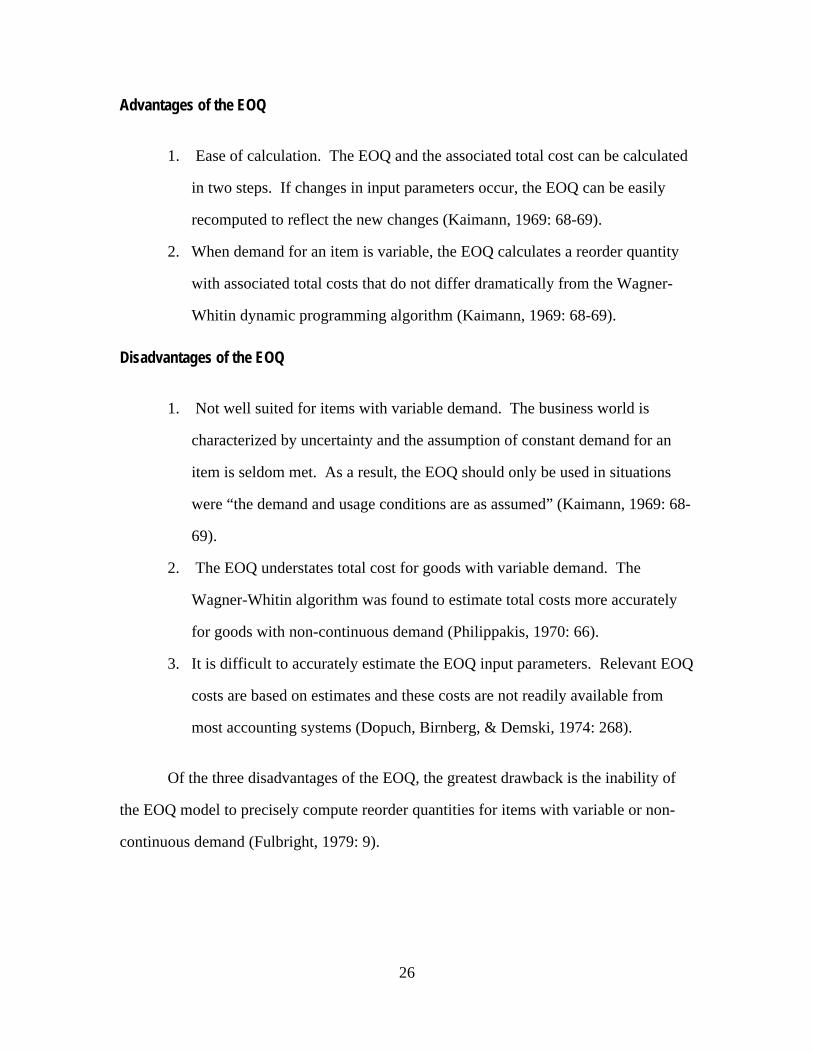
Fulbright provides an explanation of the popularity of the EOQ model, even when

the EOQ assumptions are not satisfied. By surveying numerous articles pertaining to the

use of the EOQ model, Fulbright compiled a list of the distinct advantages and

disadvantages of this inventory management technique (1979: 8). The advantages

provide some insight into the persistent use of the EOQ even under circumstances that

justify the use of a more efficient and economical inventory method. Fulbright’s list of

EOQ advantages and disadvantages, culled from relevant inventory literature, are

presented as follows:

26

Advantages of the EOQ

1. Ease of calculation. The EOQ and the associated total cost can be calculated

in two steps. If changes in input parameters occur, the EOQ can be easily

recomputed to reflect the new changes (Kaimann, 1969: 68-69).

2. When demand for an item is variable, the EOQ calculates a reorder quantity

with associated total costs that do not differ dramatically from the Wagner-

Whitin dynamic programming algorithm (Kaimann, 1969: 68-69).

Disadvantages of the EOQ

1. Not well suited for items with variable demand. The business world is

characterized by uncertainty and the assumption of constant demand for an

item is seldom met. As a result, the EOQ should only be used in situations

were “the demand and usage conditions are as assumed” (Kaimann, 1969: 68-

69).

2. The EOQ understates total cost for goods with variable demand. The

Wagner-Whitin algorithm was found to estimate total costs more accurately

for goods with non-continuous demand (Philippakis, 1970: 66).

3. It is difficult to accurately estimate the EOQ input parameters. Relevant EOQ

costs are based on estimates and these costs are not readily available from

most accounting systems (Dopuch, Birnberg, & Demski, 1974: 268).

Of the three disadvantages of the EOQ, the greatest drawback is the inability of

the EOQ model to precisely compute reorder quantities for items with variable or non-

continuous demand (Fulbright, 1979: 9).

27

DLA’s EOQ Model

DLA uses a modified version of the classic EOQ to manage its inventories. The

primary difference is DLA’s use of Quarterly Forecasted Demand (QFD) in lieu of

annual demand (D). For most items, the QFD is calculated by using a composite

forecasting method. This method employs a combination of three of nine available

individual forecasting techniques. The nine techniques are listed in Table 3-2.

Table 3-2. DLA Forecasting Methods

Technique # Forecasting Method1 Exponential Smoothing, non-program related2 Exponential Smoothing, program related3 Double Exponential Smoothing, non-program related4 Double Exponential Smoothing, program related5 Moving Average, non-program related6 Moving Average, program related7 Non Parametric, non-program related8 Non Parametric, program related9 Damped trend, non-program related


For items that experience declining demand due to the phase-out of the related

weapon system or end item, DLA uses the program related exponential smoothing

method. For other items, DLA employs a composite of the program related moving

average, exponential smoothing, and double exponential smoothing forecasting

techniques to arrive at the item’s final QFD. The final QFD is used as a variable in

DLA’s EOQ model which follows:

28

EOQDLA = 2(4QFD)A

vr

Where:

A = Fixed cost component incurred with each replenishment ($)QFD = Quarterly Forecasted Demand rate of the item (in units/unit time)v = Unit variable cost of the item ($/unit)r = Carrying charge ($/$/unit time)

To decrease computation time, DLA utilizes a “T” factor (T) to factor out the

constants in the EOQ equation. The constants are the ordering costs (A), the holding

costs (r), and the constant term “2” included in the model. DLA sets (T) equal to these

constants as follows:

T = 22A

r

Where:

T = Constant factor for the EOQDLA modelA = Fixed cost component incurred with each replenishment ($)r = Carrying charge ($/$/unit time)

The final EOQDLA model is presented below:

EOQDLA = TQFD

v =

T

2v4(QFD)v

Where:

T = Constant factor for the EOQDLA modelQFD = Quarterly Forecasted Demand rate of the item (in units/unit time)v = Unit variable cost of the item ($/unit)


29

Periodic Order Quantity

The periodic order quantity (POQ) is an alternative approach to the economic

order quantity where the EOQ is expressed as a time supply of the average item demand.

Specifically, the EOQ is divided by the average demand to arrive at an integer period

time supply.

TEOQ = EOQ

D =

2A

Dvr

Where:

A = Fixed cost component incurred with each replenishment ($)D = The average demand rate out to the horizon (N periods)v = Unit variable cost of the item ($/unit)r = Carrying charge ($/$/unit time)

Any replenishment of an item is made large enough to cover exactly the

requirements of the calculated integer number of periods. The major advantage of the

POQ is its potential to obtain lower total variable cost when there is significant

variability in the demand pattern (Silver & Peterson, 1985: 242).

Silver-Meal Heuristic

Developed in 1973 by Edward Silver and Harlan Meal, the Silver-Meal heuristic

selects order sizes for items with known, deterministic demand that varies over time

(1973: 64). The heuristic, as a simple variation of the basic EOQ model, uses the same

criteria as the EOQ to determine the replenishment quantity: the reduction of total order

and carrying costs to the lowest possible level when selecting the timing and size of

replenishments (Silver, 1979: 71).

Replenishment quantities are ordered at the beginning of every period and each

replenishment will last for T periods. The cumulative demands that occurred during the T

periods are combined to determine the order replenishment quantity or order size

30

(Tersine, 1982: 344-345). As such, the Silver-Meal criterion function, when a

replenishment arrives at the beginning of the first period and satisfies requirements to the

end of the Tth period, is presented below:

(Setup cost) + (Total carrying costs to end of period )TT


Determining each replenishment quantity over the known demand horizon is an

iterative process. The Silver-Meal heuristic evaluates the total relevant costs per unit

time, TRCUT(T), for successive T periods. Total relevant costs consist of A, the fixed

cost component incurred with each replenishment, and r, the inventory carrying charge.

The replenishment quantity for T time periods is determined when total relevant costs

begin to increase or:

TRCUT(T + 1) > TRCUT(T)

(Silver & Peterson, 1985: 234).

In Chapter II, the variability coefficient (VC) was presented to categorize demand

patterns. When an item’s VC is less than 0.2, signifying that demand for the item is

constant and continuous, Silver and Peterson recommend the use of the EOQ model to

determine replenishment quantities. However, when demand for an item is “lumpy” with

a VC greater than 0.2, they recommend the use of the Silver-Meal heuristic (Silver &

Peterson, 1985: 238).

Advantages of the Silver-Meal Heuristic

1. More useful than the basic EOQ when there is variability in the demand rate.

2. Simpler to use than dynamic programming applications, such as the Wagner-

Whitin algorithm.

31

3. Does not crucially depend on the number of forecasted demand periods.

4. Tends to use demand data of only the first few periods, recognizing that the

deterministic demand assumption becomes less reasonable as one projects further

into the future.

Disadvantages of the Silver-Meal Heuristic

1. More computationally involved than the basic EOQ.

2. Ineffective when the demand pattern drops rapidly with time over several

periods.

3. Also ineffective when there are a large number of periods having no demand.

(Silver & Peterson, 1985: 236-239)

Conclusion

An overview of the EOQ, POQ, and the Silver-Meal heuristic, three frequently

cited continuous review inventory models, was provided. The basic arithmetic equations

of the models were presented followed by an examination of the demand conditions that

favor the use of each model. Furthermore, the advantages and disadvantages of the

models were listed and discussed. This chapter provided the background necessary to

understand the methodology for the proposed simulation experiments involving the DLA

EOQ requirements model, the Periodic Order Quantity model, and Silver-Meal heuristic,

as discussed in the next chapter.

32

IV. Methodology

Introduction

This chapter will explain the methodology chosen to answer the investigative

questions posed in Chapter I. The methods outlined in this chapter will guide the

researchers throughout the research process. First, the scientific method will be

explored, followed by a discussion of why simulation will be used in this study’s

experimental design. Next, the simulation models, simulation language, and relevant

variables to be monitored in the simulation runs will be introduced. Verification and

validation of the simulation models will be discussed followed by a presentation of the

starting conditions and steady state determination of each model. Statistical procedures

to determine the number of output data runs required for conclusive results will be

summarized. Finally, a description of the paired difference test of hypothesis to analyze

the simulation output data will be presented.

The Scientific Method

Research is the formal, systematic application of the scientific method to the

study of problems. The goal of research is to explain, predict, and/or control phenomena

occurring in an experimental setting (Gay & Diehl, 1992: 6). The main distinguishing

characteristics of scientific research, according to Sekaran are presented in Table 4-1:

33

Table 4-1. Characteristics of Scientific Research

Characteristic DefinitionPurposiveness The researcher begins with a definite purpose for the researchRigor The study has a theoretical base and methodological designTestability The research lends itself to testing logically developed hypothesesReplicability The results of the tests of hypotheses should be supported when

the study is repeated in similar circumstancesPrecision How close the findings, based on a sample, are to “reality”Confidence The probability that our estimations are correct - confidence levelObjectivity The conclusions of data analysis are based on the facts resulting

from the actual data and not on subjective or emotional valuesGeneralizability The scope of applicability of research findingsParsimony Simplicity in explaining the phenomena or problems that occur

(Sekaran, 1992: 10-14)

Steps of the Scientific Method

The scientific method is an orderly process entailing five sequential steps as listed

in Table 4-2:

Table 4-2. Five Steps of the Scientific Method

Step # Description1 Selection and definition of the problem.2 Formulation of hypotheses3 Collection of data4 Analysis of data5 Statement of conclusions regarding confirmation or

disconfirmation of the hypotheses(Gay & Diehl, 1992: 6)

The importance of sequentially following the steps of the scientific method

cannot be overstated. It is the strict adherence to these steps that separates formal

research from other investigative techniques. The application of the scientific method to

problem solving lends credence to final research findings by ensuring problems are

34

carefully identified, data is systematically gathered and analyzed, and conclusions are

drawn in an objective manner.

Selection and Definition of the Problem

As presented in Chapter I, this study will focus on DSCC’s item classification

scheme and their blanket application of the DLA EOQ inventory requirements model. In

particular, the problem statement for this research is:




To help answer the above problem statement, two investigative questions were

formulated:

1. What are the results, in terms of costs and inventory levels, of applying the

DLA EOQ requirements model, the Silver-Meal Heuristic, and the Periodic Order

Quantity model to low, medium, and high demand items?

This question will quantify the costs of DSCC’s use of the EOQ requirements

model to determine stock levels for low, medium, and high demand items. DLA’s EOQ

model attempts to minimize total inventory costs by balancing ordering and holding

costs. The total inventory costs and stock levels incurred by DLA as a result of their use

of the EOQ model will be measured to compare against the total inventory costs and

stock levels DLA may experience by the implementation of a dynamic lot-sizing model

such as the Silver-Meal heuristic or the Periodic Order Quantity technique.

35

2. Which inventory model, the DLA EOQ requirements model, the Silver-Meal

Heuristic, or the Periodic Order Quantity model is more effective in minimizing

inventory costs and levels for low, medium, and high demand items?

This question will determine the most appropriate inventory requirements model

for the tested low, medium, and high demand items. The minimization of inventory

costs and levels will serve as the criterion for determining whether the DLA requirements

model, the Silver-Meal heuristic, or the Periodic Order Quantity is the most effective

inventory model for different SMCC classes. In addition, this question will investigate

whether DSCC will benefit by applying other dynamic lot-sizing models to different

inventory demand classifications instead of their present EOQ requirements model.

Experimentation

The research design chosen to answer the investigative questions in this study is

experimentation. “Experimentation is a special type of investigation used to determine

whether and in what manner variables are related to each other” (Emory, 1980: 330). The

experimental method tests hypotheses concerning cause-effect relationships (Gay &

Diehl, 1992: 382). Furthermore, this method concerns itself with determining whether

there is a relation between an independent variable (IV) and a dependent variable (DV).

This relationship is observed by manipulating the IV and detecting the presence or

absence of the DV (Emory, 1980: 331).

Experimental Design

Computer simulation is the method selected as the research technique for use in

this study. Simulation provides the opportunity to evaluate alternative ways of attaining

goals without excessive risk, cost, or time use which would be required if proposed

36

solutions were tried out on real situations before implementation. In addition, it “is a

very pragmatic and flexible technique for evaluating alternative choices in situations

where formal analytic models are inappropriate, incompatible, or incomplete in relation

to the system being studied” (House, 1977: 1-2).

Why Simulation?

Standard inventory and probabilistic models that are amenable to mathematical

analysis restrict the user to small scale systems and require simplifying assumptions that

are unrealistic for the study of a large inventory system (Wagner, 1970: 498). In

addition, an analytical solution to inventory problems is often impossible to obtain when

problems involve risk or uncertainty. “A mathematical model using the analytic

approach can become incredibly complex because of numerous interacting variables.

Simulation offers an alternative for complex problems not suitable for rigorous analytical

analysis” (Tersine, 1982: 401).

Classical analytical inventory models, such as the EOQ, are primarily developed

based on deterministic demand and lead-time assumptions. In rare instances, these

deterministic assumptions are reasonable. In most situations, however, inventory

requirements are not known for certain and require probability distributions to describe

anticipated demand. The inclusion of stochastic demand increases the complexity of

modeling. In many cases, when deterministic assumptions cannot be made about both

demand and lead-time, mathematical or analytical solutions become prohibitive (Ahadiat,

1986: 29-30). Simulation is a technique frequently used to overcome the limiting

assumptions of analytical models.

According to Nasrollah Ahadiat, the three major advantages of using simulation

for solving inventory problems are:

37

1. In many cases simulation is the only possible method for analyzing a complex

inventory system.

2. Simulation provides the ability to trace the past or future behavior of a

complex system through finely divided time intervals.

3. Using simulation, alternative inventory policies can be explored.

(Ahadiat, 1986: 32)

Simulation Language

Experimentation of the DLA EOQ requirements model, the Silver-Meal heuristic,

and the Periodic Order Quantity model will be conducted on Digital Equipment

Corporation’s (DEC) VAX 6420 mainframe computer using the Pritsker Corporation’s

SLAM II program (version 4.1). The FORTRAN subroutines to be used in conjunction

with the SLAM II computer models will be compiled and linked using the DEC VAX

FORTRAN Compiler (Version 6.1).

Simulation Models

Three inventory simulation models will be created, building on Berry and Tatge’s

1995 thesis results. While Berry and Tatge depended on the DLA forecasting method to

provide projected demand for their models, this study will incorporate a variation of the

NF1 (Naïve Forecast 1) into the models to accomplish the same task. The models will

gather demand frequency and quantity data for a full quarter. The data will then be used

to compute appropriate order quantities for the three months of next quarter using the

three ordering schemes. This demand data will then be used to actually place the

demands in the next quarter. This will allow for comparisons of results across models

without the bias of the DLA’s smoothed forecast obscuring the analysis of the models’

performance. Each of the three inventory simulation models will be run with low,

38

medium, and high demand input data to obtain the output data required to answer the

investigative questions and address the problem statement.

Relevant Variables

The relevant variables in this study are total variable cost and average on-hand

inventory. Total variable cost indicates the amount of capital invested in inventory,

representing both ordering and holding costs. It is essential for inventory managers to

reduce excessive total variable costs in light of today’s declining DoD budget. Closely

related to total variable cost is average on-hand inventory. Average on-hand inventory

directly contributes to the amount of total variable costs incurred. The greater the

amount of inventory carried from period to period generally results in higher total

variable costs during the same time-frame.

This research experiment will simulate the DLA EOQ requirements model, the

Silver-Meal heuristic, and the Periodic Order Quantity model to obtain output data to

address the investigative questions and, ultimately, the problem statement. Before

collecting data for analysis, each of the computer simulation models must be verified and

validated to ensure they are working as designed.

Verification and Validation

The computer code for the separate functions of each simulation model will be

systematically examined to verify that the models are working properly. In addition, the

SLAM II syntax check and the DEC VAX FORTRAN compiler will be relied upon to

aid in verifying the program and FORTRAN code. Finally, instead of using an input

distribution for the frequency of orders and the number of units ordered, the researchers

will substitute each SMCC’s mean value for these distributions, calculated from the input

data provided by DSCC. Each model will then be run and the output compared with an

39

analytic computation of the expected result. A match of the computer simulation results

with the analytic computations will verify the models are working properly.

Input Data

To determine the input distributions and starting conditions for the three models,

stratified random national stock number (NSN) samples from SMCCs 1, 5, and 0 will be

collected by DSCC personnel. These samples will be representative of the demand

patterns of DSCC’s low, medium, and high demand items. The data collected for each

item will include the national stock number (NSN), the past sixteen quarters of demand

data, the unit price, SMCC, lead-time, and nomenclature. This data will be analyzed to

determine the input distributions and starting conditions for each SMCC.

Input theoretical distributions for the frequency of orders and the number of units

ordered will be calculated using a statistical analysis software package. These theoretical

distributions will be evaluated using the chi-square goodness of fit test. If the chi-square

analysis indicates that theoretical distributions do not closely approximate the data, then

empirical distributions will be generated in the form of arrays for input to the models.

Additionally, the data provided by DSCC will be analyzed to determine the

starting conditions for the models. Values for unit price, lead time, reorder point (DLA

EOQ requirements model only), and on-hand inventory will be calculated and inserted

into each computer simulation model.

Steady State

According to Hoover and Perry, steady state is achieved when the probability

distribution of the state variable is no longer changing over time. It is at this time “the

state variable has reached steady state, or more correctly, reached its steady-state

distribution” (Hoover & Perry, 1990: 309). To achieve steady state, the computer

40

simulation model must be run for a certain time period so that the output is not affected

by the starting conditions. The time that elapses from the beginning of the simulation

run to the beginning of steady state is known as the transient period. Data that

accumulates during the transient period must be eliminated to ensure the final output

reflects the true steady state of the system. It is always assumed that simulation output is

generated from models that are running under steady state conditions. As such, the

transient period for computer simulation models must be determined so that observations

that occur during the transient period can be eliminated (Law & Kelton, 1991: 545).

Law and Kelton have suggested using a moving average on a measured variable

to determine the end of the transient period or the beginning of steady state. They have

observed that steady state begins when the moving average curve for the measured

variable begins to level off (Law & Kelton, 1991: 545-551). For this experiment, steady

state will be determined by running each model and applying a moving average to

measure total variable costs and average inventory. Five 200 year runs of each model

will be processed with the relevant variables collected annually. Moving averages will

be acquired from the output and analyzed to determine the length of the transient period.

Output data collection for each model will begin when the models enter into steady state.

Number of Output Data Collection Runs

According to R. Kleijnen, “If the number of simulation runs (sample size ni) is

small relative to the noise of the simulated systems (variance σ i2 ), then we obtain

inconclusive results” (1987: 46). To guard against this possibility, statistical procedures

are used to determine the number of runs that must be conducted in a simulation

experiment. In this study, the output generated for each relevant variable from the

different simulation models represents a distinct population. As such, the sample size to

41

estimate (µ1 - µ2) to within a 100(1-α)% confidence interval will be determined by the

following formula:

n = t

(.2) * (x )s

n - 1

d

/2

dx

2α

2

Where:

n = Sample sizetn-1 = t-statistic

dx = Difference of means between simulation runs

sx2

d = Variance of simulation runs

α = Desired 100(1-α)% confidence interval

In this study, the data required for insertion into the above formula will be

generated by conducting five steady state pilot runs of the simulation models for each

type of demand. The appropriate number of runs required to achieve a 95% confidence

interval will then be calculated.

Inferences About the Difference Between Two Population Means

Output data from the simulation runs will be analyzed using the paired difference

test of hypothesis. The paired difference test is used in situations where the assumption

of independent samples is invalid. In this study, independence is violated because the

quantity of average on-hand inventory directly influences the amount of total variable

costs. In other words, larger inventory levels result in greater total variable costs and

vice versa.

The paired difference test uses the difference between sample observations to

make inferences about mean µD. Mean µD is equal to the difference (µ1 - µ2): i.e., the

mean of the population (sample) of differences equals the difference between the

population (sample) means. “In many cases a paired difference experiment can provide

42

more information about the difference between population means than an independent

samples experiment. The differencing removes variability due to the dimension on

which observations are paired” (McClave & Benson, 1994: 423). The hypothesis-testing

based on the paired difference experiment is summarized below:

Ho: (µ1 - µ2) = DO or µD = 0

Ha: (µ1 - µ2) ≠ DO or µD ≠ 0

Test statistic: t = x - DO

D Ds n/

Rejection region: t < -tα/2 or t > tα/2 where tα/2 has (nD - 1) df.

(McClave & Benson, 1994: 424).

One assumption that must be met to employ the paired difference test of

hypothesis is the requirement that the differences be randomly selected from the

population of differences. This assumption will be met in this study through the use of

random number seeds in the simulation runs.

Statement of Hypotheses Conclusions

The results of the paired difference test of hypothesis will be presented. These

results will provide the data to answer the investigative questions and the problem

statement. After the investigative questions and problem statement have been addressed,

conclusions from this research and recommendations for future research will be

presented.

Summary

This chapter has explained the methodology that will be used to investigate the

investigative questions posed in Chapter I. Characteristics of the scientific method were

43

summarized followed by a discussion of why simulation will be used in this study’s

experimental design. Then, the simulation models, language, and relevant variables to be

used in the simulation runs were introduced. Verification and validation of the

simulation models was discussed followed by a presentation of the starting conditions

and steady state determination of each model. Statistical procedures to determine the

number of output data runs required for conclusive results were summarized. Finally, a

description of the paired difference test of hypothesis to analyze the simulation output

data was presented. The next chapter will explain the actual experimentation process and

results of this research.

44

V. Data Analysis

Introduction

This chapter addresses the analysis of input data, validation and verification of the

computer simulation models, the generation of output data from the models, and the

statistical techniques used to analyze both the input and output data. First, the steps used

to acquire and analyze the input data will be presented, along with the statistical methods

used for analysis. Next will be a discussion of the specific steps used to validate and

verify the computer simulation models. Finally, the techniques used to generate and

analyze the output data, including the statistical tests applied to results, will be described.

Analysis of Input Data

200 random stratified sample NSNs for each of the three SMCCs were retrieved

by Mr. James Wagner, Operations Analyst at DSCC. According to Mr. Wagner, the

samples are representative of the demand patterns experienced by items in each SMCC.

Relevant data fields retrieved for each NSN, along with sample data elements, are

provided in Appendix A. Each SMCC file was analyzed individually to acquire mean

input starting conditions and appropriate demand data for input into the simulation

models. During the initial analysis, it was discovered that there were a number of NSNs

which were included in the SMCC groupings which did not exhibit the appropriate

characteristics (number of annual demands and/or annual demand dollar value) for

inclusion in that particular SMCC (see Table 1-6 for SMCC characteristics). Cathy

Fisher from the Stock Control Directorate at DSCC indicated that the items may have

“jumped SMCCs” in the past, and that attempting to average 16 quarters of historical

data would factor-in older demands for some items which represented previous period

45

declining or increasing trends in the demand history. Since these items did not exhibit

characteristics of the SMCC to which they were now assigned (because of the inclusion

of older data) they were eliminated from consideration. Table 5-1 presents the number

of NSNs which remained in each SMCC after eliminating the atypical items.

Table 5-1. Adjusted NSN Count

SMCC NSNs1 1805 1270 154

Next, an attempt was made to acquire theoretical distributions for each SMCC for

both the mean time-between-orders and mean quantity-per-demand. Mean time-

between-orders in days for each NSN in a SMCC was calculated as follows:

NSN Mean TBO(in days) = 91

161

16

RDFi

i

/=∑

Where:TBO = Time Between OrdersRDFi = Quarterly Recurring Demand Frequency

Mean quantity-per-demand for each NSN in a SMCC was calculated as follows:

NSN Mean QPD (in units) = RDF

RDQ

i

i

i

i

=

=

∑

∑1

16

1

16

Where:QPD = Quantity Per DemandRDFi = Quarterly Recurring Demand FrequencyRDQi = Quarterly Recurring Demand Quantity

Three files containing the mean TBOs for SMCCs 1, 5, and 0 were analyzed to fit

a theoretical distribution to each data set. Theoretical distributions would enable the

46

computer simulation models to be run with an appropriate TBO and QPD input

distribution based on realistic data. However, chi-square goodness of fit tests revealed

that theoretical distributions were inappropriate for any of the TBO or QPD data sets.

Appendix B provides a sample chi-square analysis output. The individual chi-square

theoretical distribution analyses of TBO and QPD data are shown in Tables 5-2 and 5-3.

Table 5-2. Mean TBO Theoretical Distribution Evaluation by SMCC

SMCC Primary Distribution Evaluation0 Exponential Not recommended - use empirical distribution1 Uniform Not recommended - use empirical distribution5 Uniform Not recommended - use empirical distribution

Table 5-3. Mean QPD Theoretical Distribution Evaluation by SMCC

SMCC Primary Distribution Evaluation0 Exponential Not recommended - use empirical distribution1 Weibull (E) Not recommended - use empirical distribution5 Weibull (K) Use distribution with caution

An empirical distribution is used when theoretical distributions are inappropriate

or unavailable. Empirical distributions were used to represent the demand frequencies

and quantities in this research because the chi-square goodness of fit test found

theoretical distributions to be unsatisfactory. Appendix C contains a sample empirical

distribution proposed by a statistical software package for SMCC 0, along with the

appropriate SLAM code to construct the arrays required by the models.

Model Starting Conditions

Starting values for each SMCC’s unit price, lead-time, on-hand inventory, and

reorder point (for the DLA EOQ model) are represented in Appendix D and were

calculated as follows:

1. Unit price - computed using the straight mean acquired from the data set.

47

2. Lead time - calculated by adding the administrative and production lead times

for each NSN and averaging these figures.

3. On-hand inventory - one year’s average demand for a SMCC was used as a

starting inventory.

4. The starting reorder point quantity for the DLA EOQ model was calculated

by multiplying the average daily demand rate times the lead time as is

represented by the following formula:

Reorder Point (ROP) =

ARDQ

x LT

i

i

/ 4

3651

4

=∑

Where:

ARDQi = Annual Recurring Demand Quantity

Model Validation and Verification

To verify the models replicated the processes of the DLA EOQ requirements

model, the Silver-Meal heuristic, and the Periodic Order Quantity model, mean values

for each SMCC’s TBO and QPD were inserted into the respective create nodes for the

computer simulation models. For each SMCC, the performance of the computer models

was verified by running the models for one year and collecting appropriate variables at

the end of each quarter (see Appendices O through Q). This output was compared to

results that were calculated analytically and model verification was completed when

computer output based on the mean input agreed with first-year analytical results.

Number of Output Data Collection Runs

As discussed in Chapter IV, statistical procedures are necessary to determine the

number of runs that must be conducted in a simulation experiment to achieve a specified

48

level of confidence. In this study, the output data from five pilot runs was used to

calculate the number of runs required to obtain a 95% confidence interval. The pilot run

output data and the calculations to determine the number of runs required to achieve a

95% confidence level are presented in Tables 5-4 through 5-9. Based on the largest

calculated value from tables below, the researchers in this study conducted 86 simulation

runs for each model.

Table 5-4. Simulation Runs Test - SMCC 0 Average On-Hand Inventory

POQ S-M POQ EOQ EOQ S-M

Pilot Run X1 X2 X2 - X1Pilot Run X1 X2 X2 - X1

Pilot Run X1 X2 X2 - X1

1 10.2 5.4 -4.9 1 10.2 0.0 -10.2 1 0.0 5.4 5.4

2 7.1 3.9 -3.2 2 7.1 0.0 -7.1 2 0.0 3.9 3.9

3 13.5 9.5 -4.0 3 13.5 0.0 -13.5 3 0.0 9.5 9.5

4 8.1 3.0 -5.1 4 8.1 0.0 -8.1 4 0.0 3.0 3.0

5 11.7 6.8 -4.9 5 11.7 0.0 -11.7 5 0.0 6.8 6.8

Xd-4.4 Xd

-10.1 Xd5.7

sX2

d0.6 s

X2

d6.7 s

X2

d6.6

C -0.9 C -2.0 C 1.1

tn-1 2.776 tn-1 2.776 tn-1 2.776

# Runs 6.1 # Runs 12.7 # Runs 39.0

49





1 1103.0 1076.0 -27.0 1 1103.0 81.2 -1021.8 1 81.2 1076.0 994.8

2 1148.0 1113.0 -35.0 2 1148.0 81.4 -1066.6 2 81.4 1113.0 1031.6

3 1173.0 1158.0 -15.0 3 1173.0 35.5 -1137.5 3 35.5 1158.0 1122.5

4 1093.0 1082.0 -11.0 4 1093.0 99.5 -993.5 4 99.5 1082.0 982.5

5 1189.0 1182.0 -7.0 5 1189.0 30.5 -1158.5 5 30.5 1182.0 1151.5

Xd-19.0 Xd

-1075.6 Xd1056.6

sX2

d136 s

X2

d5105.1 s

X2

d5821.3

C -3.8 C -215.1 C 211.3

tn-1 2.776 tn-1 2.776 tn-1 2.776

# Runs 72.6 # Runs 0.9 # Runs 1.0





1 1.8 3.2 1.4 1 1.8 19.7 17.0 1 19.7 3.2 -16.5

2 9.1 12.6 3.5 2 9.1 22.7 13.6 2 22.7 12.6 -10.1

3 3.0 6.3 3.3 3 3.0 13.8 10.7 3 13.8 6.3 -7.4

4 4.0 5.4 1.4 4 4.0 7.0 3.0 4 7.0 5.4 -1.6

5 5.2 7.7 2.5 5 5.2 25.5 20.3 5 25.5 7.7 -17.8

Xd2.4 Xd

13.1 Xd-10.7

sX2

d1.0 s

X2

d45.7 s

X2

d44.4

C 0.5 C 2.6 C -2.1

tn-1 2.776 tn-1 2.776 tn-1 2.776

# Runs 32.9 # Runs 51.1 # Runs 74.6

Table 5-7. Simulation Runs Test - SMCC 0 Total Variable Cost




1 164.5 87.1 -77.4 1 164.5 10.6 -153.9 1 10.6 87.1 76.5

2 119.0 67.9 -51.1 2 119.0 11.9 -107.1 2 11.9 67.9 56.0

3 209.9 145.5 -64.4 3 209.9 10.9 -199.0 3 10.9 145.5 134.6

4 133.7 54.7 -79.0 4 133.7 8.4 -125.3 4 8.4 54.7 46.3

5 181.3 110.3 -71.0 5 181.3 10.6 -170.7 5 10.6 110.3 99.7

Xd-68.6 Xd

-151.2 Xd82.6

sX2

d128.6 s

X2

d1322.4 s

X2

d1265.1

C -13.7 C -30.2 C 16.5

tn-1 2.776 tn-1 2.776 tn-1 2.776

50

# Runs 5.3 # Runs 11.1 # Runs 35.7





1 6569.0 6431.0 -138.0 1 6569.0 750.0 -5819.0 1 750.0 6431.0 5681.0

2 6835.0 6598.0 -237.0 2 6835.0 747.8 -6087.2 2 747.8 6598.0 5850.2

3 6985.0 6895.0 -90.0 3 6985.0 471.7 -6513.3 3 471.7 6895.0 6423.3

4 6548.0 6481.0 -67.0 4 6548.0 858.1 -5689.9 4 858.1 6481.0 5622.9

5 7015.0 6972.0 -43.0 5 7015.0 442.7 -6572.3 5 442.7 6972.0 6529.3

Xd-115.0 Xd

-6136.3 Xd6021.3

sX2

d5881.5 s

X2

d158647.0 s

X2

d180867.5

C -23.0 C -1227.3 C 1204.3

tn-1 2.776 tn-1 2.776 tn-1 2.776

# Runs 85.7 # Runs 0.8 # Runs 1.0





1 314.2 513.4 199.2 1 314.2 2771.0 2456.8 1 2771.0 513.4 -2257.6

2 1332.0 1828.0 496.0 2 1332.0 3204.0 1872.0 2 3204.0 1828.0 -1376.0

3 487.4 970.3 482.9 3 487.4 2003.0 1515.6 3 2003.0 970.3 -1032.7

4 611.5 812.3 200.8 4 611.5 1161.2 549.5 4 1161.0 812.3 -348.7

5 769.9 114.0 344.1 5 769.9 3468.0 2698.1 5 3468.0 1114.0 -2354.0

Xd344.6 Xd

1818.4 Xd-1473.8

sX2

d20967.2 s

X2

d721523.7 s

X2

d714769.6

C 68.9 C 363.7 C -294.8

tn-1 2.776 tn-1 2.776 tn-1 2.776

# Runs 34.0 # Runs 42.0 # Runs 63.4

51

Analysis of Output Data

This study will use the paired difference test of hypotheses to test the difference

between sample observations of both average on-hand inventory and total variable cost

for each SMCC to make inferences about mean µD. The paired difference test results for

average on-hand inventory and TVC are presented below:

Average On-Hand Inventory

Average on-hand inventory represents the mean stockage level of items that

would be maintained at DLA for each inventory method and each type of demand. The

output results for this variable are summarized in Table 5-11 below:

Table 5-11. Average On-Hand Inventory Levels

Model Type of Demand Mean St. Dev.DLA EOQ - SMCC 0 Low 0.00 0.00

Silver-Meal - SMCC 0 Low 6.74 2.49POQ SMCC 0 Low 8.44 5.44

DLA EOQ - SMCC 5 Medium 12.88 7.30Silver-Meal - SMCC 5 Medium 6.89 5.50

POQ SMCC 5 Medium 5.16 4.50DLA EOQ - SMCC 1 High 62.64 23.27

Silver-Meal - SMCC 1 High 1131.91 43.34POQ SMCC 1 High 1131.63 39.81

1. Average on-hand inventory comparison of the DLA EOQ Requirements

Model-SMCC 0 and Silver-Meal Heuristic-SMCC 0.

52

Table 5-12. SMCC 0 DLA EOQ and Silver-Meal Paired Difference Test

DLA EOQ InvSMCC 0

Silver-Meal InvSMCC 0

Mean 0.00 6.74Standard Deviation 0.00 2.49X D (Silver Meal - EOQ) 6.74

t 25.07tα/2 1.97

HO: Silver-Meal - DLA EOQ = 0Ha: Silver-Meal - DLA EOQ ≠ 0

The calculated t value of 25.07 greatly exceeds the critical t value of 1.97,

indicating strong evidence that the mean on-hand inventory for the Silver-Meal model is

greater than that of the DLA EOQ model for low demand items.


Model-SMCC 0 and Periodic Order Quantity Model-SMCC 0.

Table 5-13. SMCC 0 DLA EOQ and POQ Paired Difference Test

DLA EOQ InvSMCC 0

POQ InvSMCC 0

Mean 0.00 8.44Standard Deviation 0.00 5.44X D (POQ - EOQ) 8.44

t 14.38tα/2 1.97

HO: POQ - DLA EOQ = 0Ha: POQ - DLA EOQ ≠ 0

53


indicating strong evidence that the mean on-hand inventory for the POQ model is greater

than that of the DLA EOQ model for low demand items.

3. Average on-hand inventory comparison of the Silver-Meal Heuristic-SMCC 0

and Periodic Order Quantity Model-SMCC 0.

Table 5-14. SMCC 0 Silver-Meal and POQ Paired Difference Test

Silver-MealInv SMCC 0

POQ InvSMCC 0

Mean 6.74 8.44Standard Deviation 2.49 5.44X D (POQ - Silver Meal) 1.70

t 3.09tα/2 1.97

HO: POQ - Silver Meal = 0Ha: POQ - Silver Meal ≠ 0

The calculated t value of 3.09 exceeds the critical t value of 1.97, indicating that

the mean on-hand inventory for the POQ model is greater than that of the Silver-Meal

model for low demand items.



54


DLA EOQ InvSMCC 1


Mean 62.64 1131.91Standard Deviation 23.27 43.34X D (Silver Meal - EOQ) 1069.26

t 188.54tα/2 1.97

HO: Silver Meal - EOQ = 0Ha: Silver Meal - EOQ ≠ 0

The calculated t value of 188.54 is significantly higher than the critical t value of

1.97, indicating that the mean on-hand inventory for the Silver-Meal model is greater

than that of DLA’s EOQ model for high demand items.




DLA EOQ InvSMCC 1

POQ InvSMCC 1

Mean 62.64 1131.63Standard Deviation 23.27 39.81X D (POQ - EOQ) 1068.98

t 199.63tα/2 1.97

HO: POQ - EOQ = 0Ha: POQ - EOQ ≠ 0

55

The calculated t value of 199.63 is significantly higher than the critical t value of

1.97, indicating that the mean on-hand inventory for the POQ model is greater than that

of DLA’s EOQ model for high demand items.


and Periodic Order Quantity Model-SMCC 1.


Silver-MealInv SMCC 1

POQ InvSMCC 1

Mean 1131.91 1131.63Standard Deviation 43.34 39.81X D (Silver Meal - POQ) 0.28

t 0.14tα/2 1.97

HO: Silver Meal - POQ = 0Ha: Silver Meal - POQ ≠ 0

The calculated t value of .14 is less than the critical t value of 1.97, indicating that

there is insufficient evidence to reject the null hypothesis that the mean on-hand

inventory for the POQ and the Silver-Models differ appreciably for high demand items.



56


DLA EOQ InvSMCC 5


Mean 12.88 6.89Standard Deviation 7.30 5.50X D (EOQ - Silver Meal) 5.99

t 5.96tα/2 1.97

HO: EOQ - Silver Meal = 0Ha: EOQ - Silver Meal ≠ 0


the mean on-hand inventory for the EOQ model is greater than that of the Silver-Meal

model for medium demand items.




DLA EOQ Inv SMCC 5

POQ InvSMCC 5

Mean 12.88 5.16Standard Deviation 7.30 4.50X D (EOQ - POQ) 7.72

t 8.26tα/2 1.97

HO: EOQ - POQ = 0Ha: EOQ - POQ ≠ 0

57


the mean on-hand inventory for the EOQ model is greater than that of the POQ model

for medium demand items.


and Periodic Order Quantity Model - SMCC 5.


Silver-Meal Inv SMCC 5

POQ InvSMCC 5


t 6.71tα/2 1.97



the mean on-hand inventory for the Silver-Meal model is greater than that of the POQ

model.

Total Variable Costs

Total variable costs represent DLA’s expenses to order and hold inventory. The

output results for this variable are summarized in Table 5-21 below:

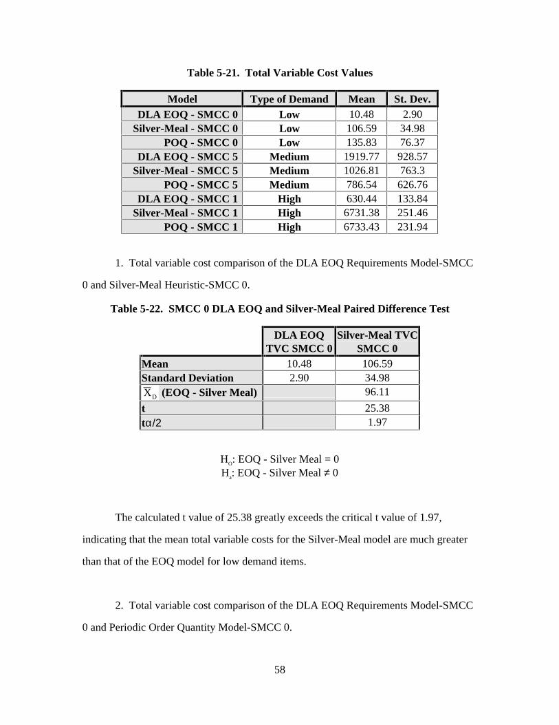
58

Table 5-21. Total Variable Cost Values

Model Type of Demand Mean St. Dev.DLA EOQ - SMCC 0 Low 10.48 2.90

Silver-Meal - SMCC 0 Low 106.59 34.98POQ - SMCC 0 Low 135.83 76.37

DLA EOQ - SMCC 5 Medium 1919.77 928.57Silver-Meal - SMCC 5 Medium 1026.81 763.3

POQ - SMCC 5 Medium 786.54 626.76DLA EOQ - SMCC 1 High 630.44 133.84

Silver-Meal - SMCC 1 High 6731.38 251.46POQ - SMCC 1 High 6733.43 231.94

1. Total variable cost comparison of the DLA EOQ Requirements Model-SMCC

0 and Silver-Meal Heuristic-SMCC 0.


DLA EOQTVC SMCC 0

Silver-Meal TVCSMCC 0


t 25.38tα/2 1.97



indicating that the mean total variable costs for the Silver-Meal model are much greater

than that of the EOQ model for low demand items.


0 and Periodic Order Quantity Model-SMCC 0.

59


DLA EOQTVC SMCC 0

POQ TVCSMCC 0


t 15.19tα/2 1.97



the mean total variable costs for the POQ model are greater than that of the EOQ for low

demand items as evidenced by the X D value of $125.35.

3. Total variable cost comparison of the Silver-Meal Heuristic-SMCC 0 and

Periodic Order Quantity Model-SMCC 0.


Silver-MealTVC SMCC 0

POQ TVCSMCC 0

Mean 106.59 135.83Standard Deviation 34.98 76.37X D (POQ - Silver Meal) 29.24

t 3.77tα/2 1.97


60


the mean total variable costs for the POQ model is greater than that of the Silver-Meal

model for low demand items as evidenced by the X D value of $29.24.




DLA EOQTVC SMCC 1


Mean 630.44 6731.38Standard Deviation 133.84 251.46X D ( Silver Meal - EOQ) 6100.94

t 184.99tα/2 1.97

HO: Silver Meal - EOQ = 0Ha: Silver Meal - EOQ ≠ 0


indicating that the mean total variable costs for the Silver-Meal model are greater than

that of the EOQ for high demand items.



61


DLA EOQTVC SMCC 1

POQ TVCSMCC 1

Mean 630.44 6733.43Standard Deviation 133.84 231.94X D ( POQ - EOQ) 6102.99

t 195.71tα/2 1.97

HO: POQ - EOQ = 0Ha: POQ - EOQ ≠ 0


indicating that the mean total variable costs for the POQ model are greater than that of

the EOQ for high demand items.





POQ TVCSMCC 1

Mean 6731.38 6733.43Standard Deviation 251.46 231.94X D ( POQ - Silver Meal) 2.05

t 0.18tα/2 1.97


The calculated t value of 0.18 is less than the critical t value of 1.97, indicating

that there is insufficient evidence to reject the null hypothesis that the mean total

variable cost for the POQ and the Silver-Meal models differ appreciably for high demand

items.

62




DLA EOQTVC SMCC 5



t 6.74tα/2 1.97



the mean total variable costs for the EOQ model are greater than that of the Silver-Meal





DLA EOQTVC SMCC 5

POQ TVCSMCC 5


t 9.28tα/2 1.97


63


the mean total variable costs for the EOQ model are greater than that of the POQ for

medium demand items.





POQ TVCSMCC 5


t 6.70tα/2 1.97



the mean total variable costs for the Silver-Meal model are greater than that of the POQ


Summary

In this chapter, the methods used to analyze the data obtained from DSCC to

arrive at model starting conditions were presented. The verification and validation

process was documented. In addition, the statistical tests performed on the output data to

64

test the research hypotheses were detailed. Chapter VI provides conclusions drawn from

this research, as well as recommendations for future research.

65

VI. Conclusions, Implications and Recommendations

Introduction

This chapter will answer the investigative questions that were postulated in

Chapter I. The information that is obtained from answering these questions will serve to

address the problem statement. Finally, research conclusions and recommendations for

future research are provided.

Problem Statement and Investigative Questions

The Chapter I problem statement and investigative questions have served to focus

the research methodology and experimental design implemented in this study. The

procedures used by the researchers were designed to gather data in an attempt to

specifically answer the investigative questions and address the problem statement. Each

of the investigative questions will be answered below using the data generated from the

simulation experiments. Then the research question will be addressed with the

information obtained from the investigative questions:

Investigative Questions

1. What are the results, in terms of costs and inventory levels, of applying the DLA EOQ

requirements model, the Silver-Meal Heuristic, and the Periodic Order Quantity model to low,

medium, and high demand items?

A summary of the results obtained from the data analysis in Chapter V is

provided in the following tables:

66

Table 6-1. Summary of Average On-Hand Inventory Results

Demand Type DLA EOQ POQ Silver-MealLow 0.00 8.44 6.74

Medium 12.88 5.16 6.89High 62.64 1131.63 1131.91

Table 6-2. Summary of Total Variable Cost Results

Demand Type DLA EOQ POQ Silver-MealLow 10.48 135.83 106.59

Medium 1919.77 786.54 1026.81High 630.44 6733.43 6731.43

As the results above indicate, a direct relationship exists between the two relevant

variables, average on-hand inventory and total variable cost. The greater the amount of

inventory that DSCC carries from one period to the next causes an increase in their

inventory holding costs. It is clear that different demand conditions produce different

results from the inventory models analyzed in this study.

The second investigative question will be anwered using the results of the

statistical analyses performed on the low, medium, and high demand categories of items

managed by DSCC.

2. Which inventory model, the DLA EOQ requirements model, the Silver-Meal Heuristic, or

the Periodic Order Quantity model is more effective in minimizing inventory costs and levels

for low, medium, and high demand items?

Low demand (SMCC 0) - Tables 6-1 and 6-2 indicate that the DLA EOQ model

clearly outperformed the POQ and Silver-Meal models in terms of TVC and average on-

67

hand inventory under low demand conditions. Statistical analysis of this demand

category revealed that the EOQ performed best, followed by the Silver-Meal heuristic

and the Periodic Order Quantity. It should be noted, however, that the DLA

requirements model never carried on-hand inventory. The original model verification

and validation process did not disclose any errors that would contribute to this outcome.

An additional thorough check of the DLA EOQ requirements model computer code did

not detect a cause. The extremely irregular demand patterns which the model

encountered during the simulation of low demand items rendered the EOQ model

incapable of maintaining a sufficient inventory balance. Because the EOQ used a

quarterly forecasted value to provide an appropriate order quantity, a significant spike in

demand in subsequent quarters would render the EOQ order quantity artificially low,

resulting in an insufficient quantity of items ordered to satisfy demands. Additionally,

the EOQ attempts to balance ordering and holding costs, but because of erratic and

limited demand, low ordering costs, and no backorder penalties, the model does not

maintain inventory in this low demand situation. As was discussed in Chapter II, the

EOQ model is subject to demand pattern and lead-time assumptions. Specifically, for the

EOQ to achieve optimal performance, demand should be constant and continuous and

lead time minimized. While numerically superior in terms of minimizing on-hand

inventory and total variable costs, the EOQ model’s inability to maintain an inventory of

low demand items could seriously degrade customer service for low demand items.

Medium demand (SMCC 5) - Statistical analysis judged the Periodic Order

Quantity as the superior model for medium demand items. This model provided the

68

lowest total variable cost and average on-hand inventory results, followed by the Silver-

Meal heuristic and the DLA EOQ model. As discussed in Chapter III, the POQ has the

potential to perform best in terms of lower total variable cost when there is variability in

the demand pattern. Medium demand provided the POQ with the opportunity to achieve

enhanced performance.

High demand (SMCC 1) - The DLA EOQ requirements model was clearly

superior in comparisons against the POQ and the Silver-Meal models. The differences

between the DLA EOQ and the other two models in terms of average on-hand inventory

and total variable cost was statistically significant, approaching an order of magnitude of

ten. Analysis of the high demand output data interestingly revealed no statistical

difference between the performance of the POQ and Silver-Meal models.

Further investigation into the performance contrast between the EOQ and the two

other models indicated that the starting conditions of the simulation experiment may have

contributed to the extreme differences. The DLA EOQ model employs a reorder point to

trigger orders when on-hand and pipeline (inbound) inventory falls to a certain level.

This reorder point is allowed to vary depending on the daily demand rate and the

replenishment lead-time. The purpose of the reorder point is to maintain a stock of

inventory to satisfy demands received during replenishment lead-time. As a result, the

EOQ effectively maintains minimal, yet sufficient on-hand inventory for high demand

items.

In contrast, neither the Periodic Order Quantity nor Silver-Meal model have a

reorder-point mechanism to signal when to place an order. All three models begin their

simulation runs with identical starting inventory levels to satisfy demands received

during the transient phase, providing for consistent comparisons across models as

discussed in Chapter IV. The EOQ must fall to a certain level before a replenishment

69

order is placed. However, since the POQ and Silver-Meal lack a reorder point

mechanism, the on-hand inventory balance is not considered when the models place

orders, making the two models extremely sensitive to the starting on-hand inventory

balance for high demand items.

Problem Statement




This study found evidence to indicate that different dynamic lot-sizing models

can provide lower total variable cost and on-hand inventory levels than the DLA EOQ

requirements model. The Periodic Order Quantity was the statistically superior model

for medium demand items. In addition, the Silver-Meal heuristic ranked second in all

three categories of demand. The DLA requirements model ranked first in both the low

and high demand categories. However, issues concerning customer service and model

starting conditions indicate the need for further research in these areas.

Recommendations for Future Research

This study identified several potential areas for future research as follows:

1. Evaluate DLA’s blanket use of QFD to forecast for all items regardless of

SMCC classification. Many forecasting models exist that may provide better results as

judged by the mean absolute deviation (MAD) accuracy measure.

2. Simulate the DLA EOQ requirements model from a customer service

perspective. Customer service measures of effectiveness can include the number of

backorders in the system and the amount of time an average backorder waits before being

70

filled. The simulation model should incorporate a monetary fine whenever backorders

occur and a daily penalty for the amount of time the backorder remains unfilled. In this

experiment, backorders were not penalized. Although the DLA EOQ requirements

model was statistically superior in the low demand, it is unclear whether this superior

performance was achieved at the expense of customer service.

Summary

This chapter answered the investigative questions proposed originally in Chapter

I. These answers were used to address this study’s problem statement. The Periodic

Order Quantity model provided lower inventory levels and total variable costs than the

DLA EOQ and the Silver-Meal models for the medium demand category. The DLA

EOQ requirements model was found to provide lower inventory levels and total variable

costs than the either the POQ or the Silver-Meal models in the low and high demand

categories. Finally, recommendations for future research were developed.

71

Appendix A. Sample of Data from DSCC

NSN NOUNUNIT

PRICE SMCC WSIC1 WSIC2 ALT PLT QFDQFDNEW

ROPQTY

2510010241054 FENDER,VEH $338.5 8 1 Z 1 24 153 45 0 1552510013175493 GRILLE,META $55.2 8 1 F 3 68 112 115 23 245

ARDQ96/2

ARDF96/2

RDQ96/2

RDQ96/1

RDQ95/4

RDQ95/3

RDF96/2

RDF96/1

RDF95/4

RDF95/3

201 154 37 17 58 89 35 13 41 65390 306 125 96 73 96 83 74 69 80

ARDQ95/2

ARDF95/2

RDQ95/2

RDQ95/1

RDQ94/4

RDQ94/3

RDF95/2

RDF95/1

RDF94/4

RDF94/3

217 187 35 31 77 74 33 27 67 60281 243 83 76 80 42 74 67 62 40

ARDQ94/2

ARDF94/2

RDQ94/2

RDQ94/1

RDQ93/4

RDQ93/3

RDF94/2

RDF94/1

RDF 93/4

RDF93/3

347 260 57 73 107 110 43 54 86 77148 131 63 54 22 9 54 48 22 7

ARDQ93/2

ARDF 93/2

RDQ93/2

RDQ93/1

RDQ92/4

RDQ92/3

RDF93/2

RDF93/1

RDF92/4

RDF92/3

390 341 90 76 130 94 71 70 117 8365 40 0 8 34 23 0 8 17 15

Acronym Glossary

NSN - National Stock NumberSMCC - Selective Management Category CodeWSIC1 - Weapon System Identification Code 1WSIC2 - Weapon System Identification Code 2ALT - Administrative Lead TimePLT - Production Lead TimeQFD - Quarterly Forecasted DemandQFD NEW - New Quarterly Forecasted DemandROP QTY - Reorder Point QuantityARDQ - Annual Recurring Demand QuantityRDQ - Recurring Demand QuantityRDF - Recurring Demand Frequency

72

Appendix B. Sample Input Distribution Analysis

Summary of Sample: Data From MQPDSMC0.DAT

Sample Characteristic ValueObservation Type Real ValuedNumber of Observations 154Minimum Observation 1.00000E-05Maximum Observation 87.8333Mean 7.28608Median 3.45000Variance 110.994Skewness 3.99975

Guided Selection Model Rankings For Sample: Data FromMQPDSMC0.DATRange of Random Variable

During the fitting process UniFit considers distributionshaving any reasonable range (not just the specified range),provided they produce values in the specified range at least99% of the time.

Specified random variable range Between 0. and 87.8333

Relative Evaluation of Candidate Models

Relative Score Random Variable Range Models (0-100) (if different from specified)1-Exponential 75.0 At least 0.2-Gamma 75.0 At least 0.3-Weibull 75.0 At least 0.4-Uniform 18.85-Inverse Gaussian 6.3 At least 0.

Current Primary Model

1-Exponential

Absolute Evaluation of the Primary Model

Based on a heuristic evaluation, we do not recommend usingthe primary model. If you are doing simulation, then youshould use an empirical distribution rather than the primarymodel (unless you can show that it is good).

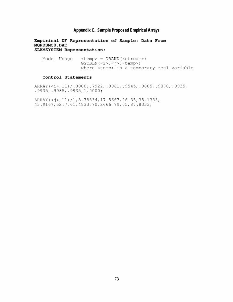
73

Appendix C. Sample Proposed Empirical Arrays

Empirical DF Representation of Sample: Data FromMQPDSMC0.DATSLAMSYSTEM Representation:

Model Usage <temp> = DRAND(<stream>) GGTBLN(<i>,<j>,<temp>) where <temp> is a temporary real variable

Control Statements

ARRAY(<i>,11)/.0000,.7922,.8961,.9545,.9805,.9870,.9935,.9935,.9935,.9935,1.0000;

ARRAY(<j>,11)/1,8.78334,17.5667,26.35,35.1333,43.9167,52.7,61.4833,70.2666,79.05,87.8333;

74

Appendix D. Starting Conditions for Each SMCC

SMCCAnnualDemand

Frequency MTBO MQPD

XX(1)Annual

Demand

XX(15)UnitPrice

XX(6)Total

Lead-Time

XX(3)ROPQ

1 259 1.41 12.88 3315 $ 58.58 190 17265 7.2 51.05 6.32 45.5 $1,408.61 300 380 1.21 299.80 7.29 8.82 $ 141.30 190 5

Acronym Glossary

SMCC - Selective Management Category CodeMTBO- Mean Time Between OrdersMQPD- Mean Quantity Per DemandROPQ - Reorder Point Quantity

75

Appendix E. Input Arrays

The following input arrays were inserted into the SMCC 0, 1, and 5 simulation

models to generate the time between orders (TBO) and the mean quantity per demand

(QPD).

SMCC 0

ARRAY(1,11)/.0000,.3117,.7468,.7987,.8961,.9610,.9611,.9612, .9613,.9614,1.0000;ARRAY(2,11)/1.0,145.6,291.2,436.8,582.4,728.,873.6, 1019.2,1164.8,1310.4,1456.;ARRAY(3,11)/.0000,.7922,.8961,.9545,.9805,.9870,.9935,.9936, .9937,.9938,1.0000;ARRAY(4,11)/1.0,8.78334,17.5667,26.35,35.1333, 43.9167,52.7,61.4833,70.2666,79.05,87.8333;

SMCC 1

ARRAY(1,11)/.0000,.0889,.2167,.3778,.5111,.6556,.7500,.8556, .9611,.9944,1.0000;ARRAY(2,11)/.07731,.40352,.72973,1.05594,1.38215,1.70836, 2.03456,2.36077,2.68698,3.01319,3.3394;ARRAY(3,11)/.0000,.8667,.9222,.9444,.9500,.9778,.9833,.9834, .9835,.9944,1.0000;ARRAY(4,11)/1.22611,19.6255,38.025,56.4244,74.8239,93.2233, 111.623,130.022,148.422,166.821,185.221;

SMCC 5

ARRAY(1,11)/.0000,.2047,.3543,.5433,.6614,.7480,.8110,.8661, .9449,.9606,1.0000;ARRAY(2,11)/19.158,28.4422,37.7264,47.0106,56.2948,65.579, 74.8632,84.1474,93.4316,102.716,112.;ARRAY(3,11)/.0000,.9055,.9528,.9764,.9843,.9844,.9921,.9922, .9923,.9924,1.0000;ARRAY(4,11)/1.00001,13.8643,26.7286,39.5929,52.4572,65.3215,

78.1857,91.05,103.914,116.779,129.643;

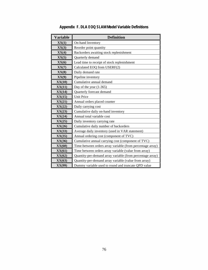
76

Appendix F. DLA EOQ SLAM Model Variable Definitions

Variable DefinitionXX(1) On-hand Inventory

XX(3) Reorder point quantity

XX(4) Backorders awaiting stock replenishment

XX(5) Quarterly demand

XX(6) Lead time to receipt of stock replenishment

XX(7) Calculated EOQ from USERF(2)

XX(8) Daily demand rate

XX(9) Pipeline inventory

XX(10) Cumulative annual demand

XX(11) Day of the year (1-365)

XX(14) Quarterly forecast demand

XX(15) Unit Price

XX(21) Annual orders placed counter

XX(22) Daily carrying cost

XX(23) Cumulative daily on-hand inventory

XX(24) Annual total variable cost

XX(25) Daily inventory carrying rate

XX(26) Cumulative daily number of backorders

XX(33) Average daily inventory (used in VAR statement)

XX(35) Annual ordering cost (component of TVC)

XX(36) Cumulative annual carrying cost (component of TVC)

XX(60) Time-between orders array variable (from percentage array)

XX(61) Time between orders array variable (value from array)

XX(62) Quantity-per-demand array variable (from percentage array)

XX(63) Quantity-per-demand array variable (value from array)

XX(99) Dummy variable used to round and truncate QPD value

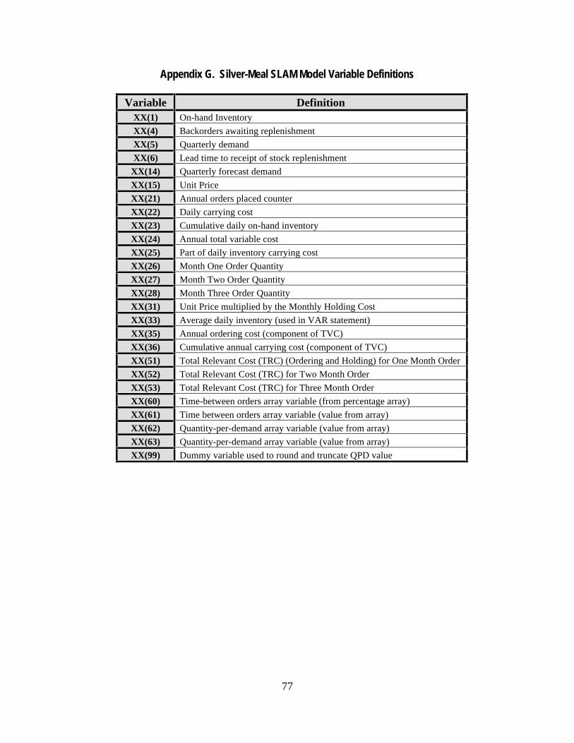
77

Appendix G. Silver-Meal SLAM Model Variable Definitions


XX(4) Backorders awaiting replenishment




XX(15) Unit Price





XX(25) Part of daily inventory carrying cost

XX(26) Month One Order Quantity

XX(27) Month Two Order Quantity

XX(28) Month Three Order Quantity

XX(31) Unit Price multiplied by the Monthly Holding Cost




XX(51) Total Relevant Cost (TRC) (Ordering and Holding) for One Month Order

XX(52) Total Relevant Cost (TRC) for Two Month Order

XX(53) Total Relevant Cost (TRC) for Three Month Order






78

Appendix H. Periodic Order Quantity SLAM Model Variable Definitions


XX(4) Backorders awaiting replenishment




XX(15) Unit Price





XX(25) Part of daily inventory carrying cost

XX(26) Month One Order Quantity

XX(27) Month Two Order Quantity

XX(28) Month Three Order Quantity








XX(70) Monthly Order Quantity

XX(71) Calculated value from Periodic Order Quantity formula


79

Appendix I. DLA EOQ SLAM Model

Comments are provided (in italics and under applicable lines of code) for each section

of the model as to its purpose and function.

I. Control Statement

GEN,GOULET&ROLLMAN,EOQ0,9/1/1996,5,N,N,Y/Y,N,Y/1,132;

Model authors, title, date, number of runs (1).

LIMITS,1,5,100000;

Limits statement; number of files, attribute number used, file space required.

ARRAY(1,11)/.0000,.3117,.7468,.7987,.8961,.9610,.9611,.9612,.9613,.9614, 1.0000;ARRAY(2,11)/1.0,145.6,291.2,436.8,582.4,728.,873.6,1019.2, 1164.8,1310.4,1456.;

Input arrays; time between orders.

ARRAY(3,11)/.0000,.7922,.8961,.9545,.9805,.9870,.9935,.9936,.9937,.9938, 1.0000;ARRAY(4,11)/1.0,8.78334,17.5667,26.35,35.1333,43.9167,52.7, 61.4833,70.2666,79.05,87.8333;

Input arrays; quantity per demand.

SEEDS,53060595(1),49626694(2);

Seeds statements for independent starting conditions.

INITIALIZE,,72800,Y;

Initialize statement; run for 100 years

;MONITOR,CLEAR,73000;;MONITOR,SUMRY,73365,365,Y;

Monitor clear and summary statements.

INTLC,XX(15)=142,XX(6)=190,XX(1)=15;

Starting conditions; EOQ, unit price, lead time, reorder point, on-hand inventory.

RECORD,TNOW,TIME,,T,364,,,Y;

Record statement; recorded variable, label, table output, interval (days).

;VAR,XX(14),Q,QFD;;VAR,XX(5),D,ACTUAL;VAR,XX(33),O,AVGINV;;VAR,XX(4),B,BACKORD;

80

VAR,XX(24),C,TVC

Variable statements; Variable of interest, plot label, output label.

TIMST,XX(1),XX1 OH INV;TIMST,XX(2),XX2 START EOQ;TIMST,XX(3),XX3 ROP;TIMST,XX(4),XX4 AVG BO;TIMST,XX(5),XX5 QRTLY DMD;TIMST,XX(7),XX7 USERF2 EOQ;TIMST,XX(8),XX8 DDR;TIMST,XX(9),XX9PPLN INV;TIMST,XX(10),XX10CUM DEMAND;TIMST,XX(11),XX11CUM DAYS;TIMST,XX(14),XX14QFD;TIMST,XX(21),XX21ORDERS PLACED;TIMST,XX(22),XX22DAIL CAR CST;TIMST,XX(36),XX36CUM CAR COST

Initiation of measurement for time persistent variables (measured every day).

NETWORK;

Network statement; Calls SLAM network.

II. Demand Generation and Issue/Backorder Process

DMND CREATE; ACTIVITY; ASSIGN,XX(60)=DRAND(5),XX(61)=GGTBLN(1,2,XX(60)); ACTIVITY,XX(61),,DMND; ACTIVITY,,,QTY;

Demand creation; One entity created, calls empirical arrays for time between order, entity runs assigned time, reenterscreate node to begin process again. Cloned entity from assign node sent to QTY assign node for calculation of quantity perdemand.

QTY ASSIGN,XX(62)=DRAND(5),XX(63)=GGTBLN(3,4,XX(62)),XX(99)=XX(63)+0.5, II=XX(99),ATRIB(5)=II,2;

Quantity per demand assignment; entity assigned quantity from second set of empirical arrays, number truncated, quantityassigned to attribute.

ACTIVITY,,,MLR; ACTIVITY,91,,DDR;

Send one clone to update quarterly forecasted demand. The other entity goes one quarter into the future to provide samedemand pattern and quantity.

MLR UNBATCH,5,1; ACTIVITY;

Unbatch node; Reads quantity assigned to attribute, generates corresponding number of entities representing number ofitems in order.

ASSIGN,XX(14)=XX(14)+1; ACTIVITY,,,END;

81

Update quarterly forecasted demand variable with order quantity, provides to EOQ formula in subroutine. Entityterminates.

DDR UNBATCH,5,1; ACTIVITY;QTR ASSIGN,XX(5)=XX(5)+1,XX(10)=XX(10)+1,1;

Increment quarterly and cumulative demand by number of entities in order.

ACTIVITY,,XX(1).GT.0,INV;

If there sufficient inventory to fill requisition from shelf, go to the issue inventory node.

ACTIVITY,,,BACK;

If not, go to the back order node.

INV ASSIGN,XX(1)=XX(1)-1,1;

Issue and decrement on hand inventory counter.

ACTIVITY;END TERMINATE;

Entity dies.

BACK ASSIGN,XX(4)=XX(4)+1,1;

Increment number of backorders.

ACTIVITY,,,END;

Entity dies.

III. Replenishment Cyc1e: Daily releveling, order placement, order receipt, dailyadjustment of variables.

REPL CREATE,1,,1,,1; ACTIVITY;

Create one entity every day to check inventory levels and adjust values of specific variables.

ZAAB ASSIGN,XX(25)=.1/364,XX(22)=XX(1)*XX(15)*XX(25), XX(36)=XX(36)+XX(22),XX(11)=XX(11)+1,XX(26)=XX(26)+XX(4), XX(23)=XX(23)+XX(1),1;

Compute daily inventory carrying cost, increment: cumulative annual carrying cost, day of the current year, cumulativenumber of backorders, cumulative daily on-hand inventory.

ACTIVITY; GOON,1; ACTIVITY,,XX(7).EQ.0,END; ACTIVITY,,XX(1)+XX(9).LE.XX(3);

Go to CUM node if on-hand and pipeline inventory less than reorder point quantity.

ACTIVITY,,,INFO;

82

If not, go to INFO node to collect daily on-hand inventory statistics.

CUM ASSIGN,XX(21)=XX(21)+1,1;

Increment annual orders placed counter.

ACTIVITY;EOQ ASSIGN,ATRIB(2)=XX(7),XX(9)=XX(9)+ATRIB(2),1;

Place order by setting entities second attribute equal to the most recently calculated EOQ quantity, increment pipelinequantity by same.

ACTIVITY,XX(6);

Entities wait lead time for order arrival.

PREI COLCT,XX(1),PRE REPLIN INV;

Collect pre-inventory replenishment statistics on on-hand inventory.

ACTIVITY;PREB COLCT,XX(4),PRE REPLEN BO;

Collect pre-inventory replenishment statistics on backorders.

ACTIVITY,,,PLDEC;

Go to pipeline decrement node to record shipment receipt.

ACTIVITY;INFO COLCT,XX(1),AVG INV;

Collect statistics on on-hand inventory.

ACTIVITY,,,END;

Entity dies.

PLDEC ASSIGN,XX(9)=XX(9)-ATRIB(2),1;

Decrement pipeline inventory by received shipment quantity.

ACTIVITY,,ATRIB(2).GE.XX(4),MORE;

If quantity received is greater than backorder quantity, go to MORE node.

ACTIVITY,,,LESS;

If quantity received is less than backorder quantity, go to LESS node.

MORE ASSIGN,XX(1)=XX(1)+ATRIB(2)-XX(4),XX(4)=0,1;

Increment on-hand inventory by shipment received quantity then decrement by backorder quantity if quantity in theshipment was more than the quantity of backorders.

ACTIVITY,,,END;

83

Entity dies.

LESS ASSIGN,XX(4)=XX(4)-ATRIB(2);

Decrement shipment received quantity from total backorders if the quantity in the shipment was less than the quantity ofbackorders.

ACTIVITY,,,END;

Entity dies.

IV. Quarterly calculation of forecasted demand, eoq, reorder point, and update ofvariables

CREATE,,,1,1,1; ACTIVITY,91; delay one quarter

Create one entity at time zero, it waits one quarter before it triggers recalculation of variables.

DATA COLCT,XX(5),QTRLY DMD; ACTIVITY;

Collect statistics on quarterly demand.

USER ASSIGN,XX(8)=XX(10)/XX(11),XX(3)=USERF(1), XX(7)=USERF(2),XX(5)=0,1; ACTIVITY;

Compute daily demand rate, new reorder point quantity, and rounded (up) eoq by calling fortran subroutine. Originalmodel did not calculate integer values for EOQ.

AVGE COLCT,XX(7),AVG EOQ,,1;

Collect statistics on EOQ.

ACTIVITY,91,,DATA;

Entity waits 91 days (one quarter) and is sent back to the create node DATA to begin the process again.

V. Annual computation of TVC and daily average backorders; annual variablescleared.

YEAR CREATE,364,364,,,1; ACTIVITY; ASSIGN,XX(35)=XX(21)*5.2,XX(23)=XX(23)/365, XX(26)=XX(26)/365,XX(24)=XX(35)+XX(36),XX(33)=XX(23), XX(34)=XX(26),XX(21)=0,XX(36)=0,XX(23)=0, XX(26)=0; ACTIVITY;

Compute ordering cost, daily on hand inventory, average daily backorders, TVC, VAR statement daily inventory andbackorders, clearing of annual variables.

CTVC COLCT,XX(24),TVC,,1; ACTIVITY;CINV COLCT,XX(33),INV,,1; ACTIVITY;

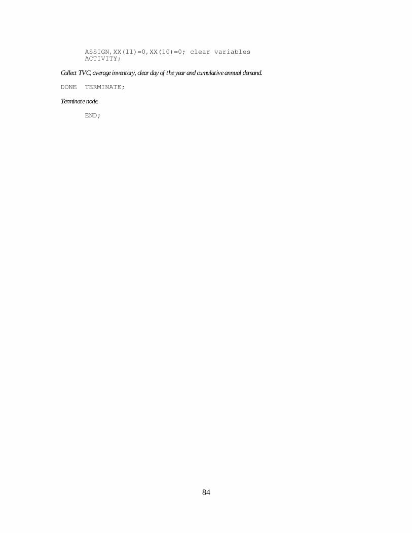
84

ASSIGN,XX(11)=0,XX(10)=0; clear variables ACTIVITY;

Collect TVC, average inventory, clear day of the year and cumulative annual demand.

DONE TERMINATE;

Terminate node.

END;

85

Appendix J: DLA EOQ SLAM Subroutine Fortran Code


of the model as to its purpose and function, as well as explanation of differences from the

original code, if applicable.

PROGRAM MAIN DIMENSION NSET(1000000) PARAMETER(MEQT=100,MSCND=25,MENTR=25,MRSC=75,MARR=50, 1 MGAT=25,MHIST=50,MCELS=500,MCLCT=50,MSTAT=50,MEQV=100, 2 MATRB=100,MFILS=100,MPLOT=10,MVARP=10,MSTRM=10, 3 MACT=100,MNODE=500,MITYP=50,MMXXV=100) PARAMETER(MVARP1=MVARP+1) COMMON/SCOM1/ATRIB(MATRB),DD(MEQT),DDL(MEQT),DTNOW,II,MFA, 1 MSTOP,NCLNR,NCRDR,NPRNT,NNRUN,NNSET,NTAPE,SS(MEQT), 2 SSL(MEQT),TNEXT,TNOW,XX(MMXXV) COMMON QSET(1000000) EQUIVALENCE(NSET(1),QSET(1)) NNSET=1000000 NCRDR=5 NPRNT=6 NTAPE=7 CALL SLAM STOP ENDCC FUNCTION USERF(IFN) PARAMETER(MEQT=100,MSCND=25,MENTR=25,MRSC=75,MARR=50, 1 MGAT=25,MHIST=50,MCELS=500,MCLCT=50,MSTAT=50,MEQV=100, 2 MATRB=100,MFILS=100,MPLOT=10,MVARP=10,MSTRM=10, 3 MACT=100,MNODE=500,MITYP=50,MMXXV=100) PARAMETER(MVARP1=MVARP+1) COMMON/SCOM1/ATRIB(MATRB),DD(MEQT),DDL(MEQT),DTNOW,II,MFA, 1 MSTOP,NCLNR,NCRDR,NPRNT,NNRUN,NNSET,NTAPE,SS(MEQT), 2 SSL(MEQT),TNEXT,TNOW,XX(MMXXV)C GOTO (10,20,30),IFNC10 I=XX(8)*XX(6) USERF=I GOTO 40

USERF1 called from model. Calculation of reorder point quantity (daily demand rate times lead time).

C20 R=20.396*(SQRT(XX(14)/XX(15))) J=INT(R+.5) USERF=J GOTO 40

USERF2 called from model. Calculation of EOQ plus .5 and truncate to provide integer value.

C30 IF (XX(23).LE.0.) THEN

86

XX(23)=0 GOTO 39 ENDIF

Artifact from original model; zeroes out cumulative daily on-hand inventory if becomes negative.

39 USERF=1C40 RETURN END

End subroutine and return to model.

87

Appendix K. Silver-Meal SLAM Model


of the model as to its purpose and function, as well as explanation of differences from the

original code, if applicable.

I. Control Statement

GEN,Goulet and Rollman,SMM0,9/1/1996,5,N,N,Y/Y,N,Y/1,132;

Model authors, title, date, number of runs (1).

LIMITS,2,5,100000;


ARRAY(1,11)/.0000,.3117,.7468,.7987,.8961,.9610,.9611,.9612,.9613,.9614, 1.0000;ARRAY(2,11)/1.0,145.6,291.2,436.8,582.4,728.,873.6,1019.2,1164.8, 1310.4,1456.;

Input arrays; time between orders.

ARRAY(3,11)/.0000,.7922,.8961,.9545,.9805,.9870,.9935,.9936,.9937,.9938, 1.0000;ARRAY(4,11)/1.0,8.78334,17.5667,26.35,35.1333,43.9167,52.7,61.4833, 70.2666,79.05,87.8333;


SEEDS,53060595(1),49626694(2);

Seeds statements for independent starting conditions.




Inactive monitor clear and summary statements used during model validation process.

INTLC,XX(15)=142,XX(6)=190,XX(1)=9

Starting conditions; unit price, lead time, on-hand inventory.



;VAR,XX(14),Q,QFD;

88

;VAR,XX(5),D,ACTUAL;VAR,XX(33),O,OHINV;;VAR,XX(4),B,BACKORD;VAR,XX(24),T,TVC;


TIMST,XX(1),XX1 OH INVTIMST,XX(2),XX2 START EOQTIMST,XX(3),XX3 ROPTIMST,XX(4),XX4 AVG BOTIMST,XX(5),XX5 QRTLY DMDTIMST,XX(7),XX7 USERF2 EOQTIMST,XX(8),XX8 DDRTIMST,XX(9),XX9PPLN INVTIMST,XX(10),XX10CUM DEMANDTIMST,XX(11),XX11CUM DAYSTIMST,XX(14),XX14QFDTIMST,XX(21),XX21ORDERS PLACEDTIMST,XX(22),XX22DAIL CAR CSTTIMST,XX(36),XX36CUM CAR COSTTIMST,XX(23),XX23AVG ANN INVTIMST,XX(24),XX24TVCTIMST,XX(25),XX25DAYS INV TAKENTIMST,XX(26),XX26QT1 VALUE;TIMST,XX(27),XX27QT2 VALUE;TIMST,XX(28),XX28QT3 VALUE;TIMST,XX(36),XX36CUM CARCOST;TIMST,XX(51),XX51SMT1TIMST,XX(52),XX52SMT2TIMST,XX(53),XX53SMT3

Initiation of measurement for time persistent variables.

NETWORK;

Network statement; Calls SLAM network.

II. Demand Generation and Issue/Backorder Process

DMND CREATE; ACTIVITY; ASSIGN,XX(60)=DRAND(5),XX(61)=GGTBLN(1,2,XX(60)); ACTIVITY,XX(61),, DMND; ACTIVITY,,, QTY;


QTY ASSIGN,XX(62)=DRAND(5),XX(63)=GGTBLN(3,4,XX(62)),XX(99)=XX(63)+0.5, II=XX(99),ATRIB(5)=II;


ACTIVITY,91,,TIM;

Batched entity sent one quarter into the future to provide identical demand frequencies and quantities.

89

ACTIVITY,,,DDR;

Send cloned entity to udate forecasted demand variable used in subroutine to calculate EOQ.

DDR UNBATCH,5,1; ACTIVITY;QTR ASSIGN,XX(14)=XX(14)+1,1; ACTIVITY,,,END;

Unbatch order quanity and update forecasted demand variable. Entity terminates.

TIM UNBATCH,5,1; ACTIVITY,,,TOM;

Unbatch order quantity to initiate fill or backorder process.

TOM ASSIGN,XX(5)=XX(5)+1,1;

Increment quarterly demand by number of entities in order.

ACTIVITY,,XX(1).GT.0.;


ACTIVITY,,,BACK;





Entity dies.

BACK ASSIGN,XX(4)=XX(4)+1,1;

Increment number of backorders.

ACTIVITY,,,END;

Entity dies.

III. Variable Update Process

REPL CREATE,1,,1,,2; ACTIVITY; ACTIVITY,,,INFO;ZAAB ASSIGN,XX(25)=.1/364,XX(22)=XX(1)*XX(15)*XX(25), XX(36)=XX(36)+XX(22),XX(22)=0,XX(23)=XX(23)+XX(1); ACTIVITY,,,END;

Calculate daily holding rate, daily holding cost, cumulative holding cost, clear daily, increment cumulative inventory.

90

IV. Quarterly Update of Silver-Meal Variables and Order Placement

SMM CREATE,91,,1,,1; ACTIVITY;

Create only one entity 91 days into the simulation to trigger the Silver-Meal ordering process and recalculation of variables.

QT1 ASSIGN,ATRIB(2)=XX(26),2; ACTIVITY,XX(6),,REN1;

Order the quantity calculated by the FORTRAN Silver-Meal heuristic for the first month of present quarter. Wait lead-time for order arrival and go to order receipt node REN1.

ACTIVITY,30,,QT2;

Send cloned quantity on 30 day trek to second month order node

ACTIVITY,,ATRIB(2).GT.0,ORDR;

If monthly order quantity is calculated at 0, don’t increment orders placed variable.

REN1 GOON,1; ACTIVITY/24,,ATRIB(2).GE.XX(4),MORE;


ACTIVITY/25,,,LESS;




ACTIVITY,,,END;

Entity dies.



ACTIVITY,,,END;

Entity dies.

QT2 ASSIGN,ATRIB(2)=XX(27),2; ACTIVITY,XX(6),ATRIB(2).GT.0,REN1;

Order the quantity calculated by the FORTRAN Silver-Meal heuristic for the second month of present quarter if there was,in fact, an order quantity calculated. Wait lead-time for order arrival and go to order receipt node REN1.

ACTIVITY,30,,QT3;

91

Send cloned quantity on 30 day trek to third month order node


If monthly order quantity is greater than 0, increment orders placed variable.

QT3 ASSIGN,ATRIB(2)=XX(28),2;ACTIVITY/28,XX(6),ATRIB(2).GT.0,REN1; goto REN1

Order the quantity calculated by the FORTRAN Silver-Meal heuristic for the third month of present quarter if there was,in fact, an order quantity calculated. Wait lead-time for order arrival and go to order receipt node REN1.



ACTIVITY,,,END;

Send cloned quantity to END terminate node

ORDR ASSIGN,XX(21)=XX(21)+1; ACTIVITY,,,END;

Increment cumulative order quantity. Entity dies.

V. Annual computation of TVC and daily average backorders; annual variablescleared.

YEAR CREATE,364,364,,,1; ACTIVITY; ASSIGN,XX(35)=XX(21)*5.2,XX(24)=XX(35)+XX(36),XX(23)=XX(23)/365, XX(21)=0,XX(33)=XX(23),XX(36)=0,XX(21)=0,XX(23)=0; ACTIVITY;

Compute ordering cost and daily on hand inventory, and TVC, clearing of annual variables.

CTVC COLCT,XX(24),TVC,,1; ACTIVITY;

Collect TVC.

CINV COLCT,XX(33),INV,,1; ACTIVITY;

Collect average inventory.

DONE TERMINATE;

Terminate node.

END;FIN

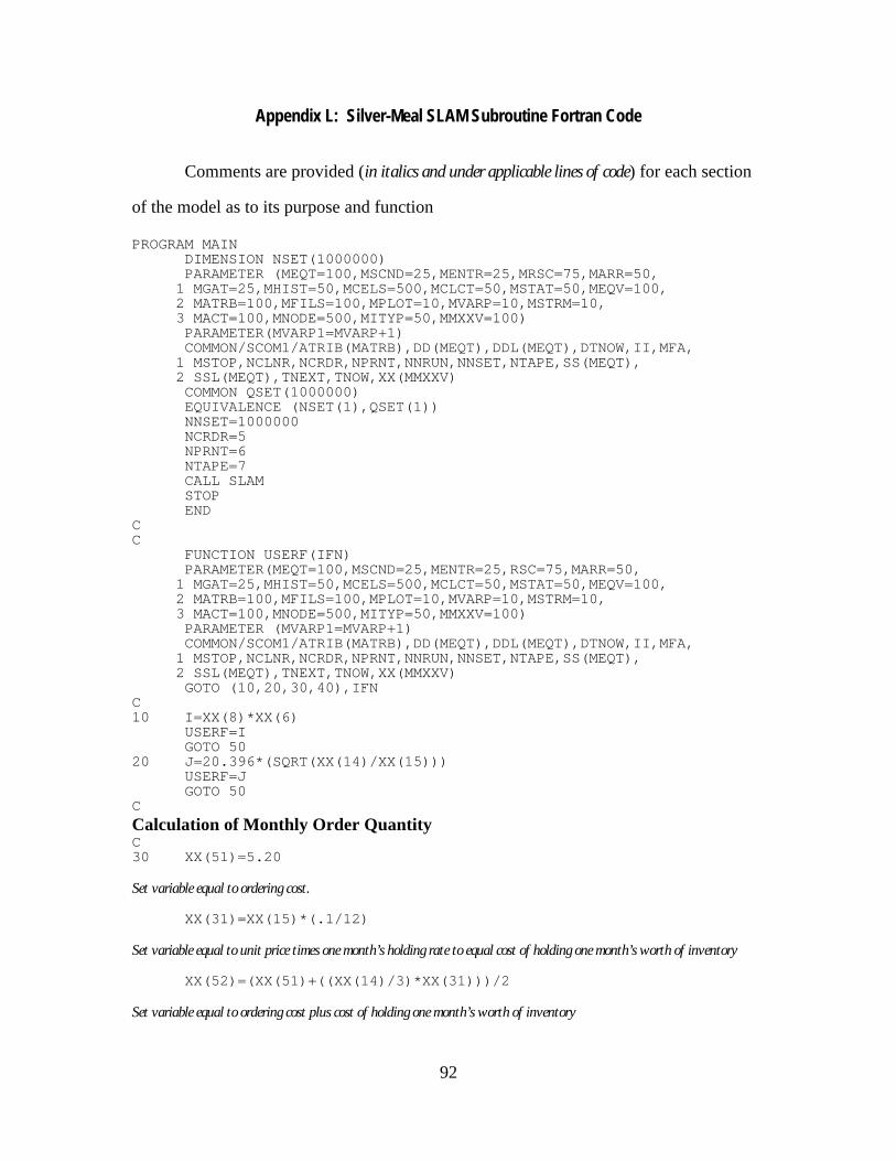
92

Appendix L: Silver-Meal SLAM Subroutine Fortran Code


of the model as to its purpose and function

PROGRAM MAIN DIMENSION NSET(1000000) PARAMETER (MEQT=100,MSCND=25,MENTR=25,MRSC=75,MARR=50, 1 MGAT=25,MHIST=50,MCELS=500,MCLCT=50,MSTAT=50,MEQV=100, 2 MATRB=100,MFILS=100,MPLOT=10,MVARP=10,MSTRM=10, 3 MACT=100,MNODE=500,MITYP=50,MMXXV=100) PARAMETER(MVARP1=MVARP+1) COMMON/SCOM1/ATRIB(MATRB),DD(MEQT),DDL(MEQT),DTNOW,II,MFA, 1 MSTOP,NCLNR,NCRDR,NPRNT,NNRUN,NNSET,NTAPE,SS(MEQT), 2 SSL(MEQT),TNEXT,TNOW,XX(MMXXV) COMMON QSET(1000000) EQUIVALENCE (NSET(1),QSET(1)) NNSET=1000000 NCRDR=5 NPRNT=6 NTAPE=7 CALL SLAM STOP ENDCC FUNCTION USERF(IFN) PARAMETER(MEQT=100,MSCND=25,MENTR=25,RSC=75,MARR=50, 1 MGAT=25,MHIST=50,MCELS=500,MCLCT=50,MSTAT=50,MEQV=100, 2 MATRB=100,MFILS=100,MPLOT=10,MVARP=10,MSTRM=10, 3 MACT=100,MNODE=500,MITYP=50,MMXXV=100) PARAMETER (MVARP1=MVARP+1) COMMON/SCOM1/ATRIB(MATRB),DD(MEQT),DDL(MEQT),DTNOW,II,MFA, 1 MSTOP,NCLNR,NCRDR,NPRNT,NNRUN,NNSET,NTAPE,SS(MEQT), 2 SSL(MEQT),TNEXT,TNOW,XX(MMXXV) GOTO (10,20,30,40),IFNC10 I=XX(8)*XX(6) USERF=I GOTO 5020 J=20.396*(SQRT(XX(14)/XX(15))) USERF=J GOTO 50C

Calculation of Monthly Order QuantityC30 XX(51)=5.20

Set variable equal to ordering cost.

XX(31)=XX(15)*(.1/12)

Set variable equal to unit price times one month’s holding rate to equal cost of holding one month’s worth of inventory

XX(52)=(XX(51)+((XX(14)/3)*XX(31)))/2

Set variable equal to ordering cost plus cost of holding one month’s worth of inventory

93

XX(53)=(XX(51)+((XX(14)/3)*(XX(31)))+(((2*XX(14))/3)*(XX(31))))/3

Set variable equal to ordering cost plus cost of holding 2 month’s worth of inventory.

IF (XX(52).GT.XX(51)) GOTO 31 GOTO 3231 IF (XX(53).GT.XX(52)) GOTO 36 GOTO 3232 IF (XX(52).LT.XX(51)) GOTO 33 GOTO 3433 IF (XX(53).GT.XX(52)) GOTO 37 GOTO 3434 IF (XX(53).LT.XX(51)) GOTO 35 GOTO 3835 IF (XX(53).LT.XX(52)) GOTO 38 GOTO 38

Series of IF statements to select lowest cost ordering policy for the next quarter.

36 XX(26)=XX(14)/3 XX(27)=XX(14)/3 XX(28)=XX(14)/3 XX(26)=INT(XX(26)+.5) XX(27)=INT(XX(27)+.5) XX(28)=INT(XX(28)+.5) XX(21)=XX(21)+3 GOTO 39

Order one month’s worth of inventory each month of the quarter. Round up and truncate order quantities.

37 XX(26)=(2*XX(14))/3 XX(27)=0 XX(28)=XX(14)/3 XX(26)=INT(XX(26)+.5) XX(28)=INT(XX(28)+.5) XX(21)=XX(21)+2 GOTO 39

Order 2 month’s worth of inventory the first month and one month’s worth the third month..

38 XX(26)=XX(14) XX(27)=0 XX(28)=0 XX(26)=INT(XX(26)+.5) XX(21)=XX(21)+1 GOTO 39

Order 3 month’s worth of inventory the first month.

39 USERF=1 GOTO 5040 IF (XX(23).LE.0) GOTO 41 GOTO 4941 XX(23)=049 USERF=150 RETURN

Return to SLAM model.

END

94

End FORTRAN subroutine.

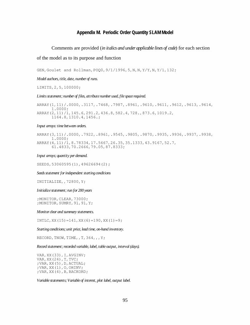
95

Appendix M. Periodic Order Quantity SLAM Model


of the model as to its purpose and function

GEN,Goulet and Rollman,POQ0,9/1/1996,5,N,N,Y/Y,N,Y/1,132;

Model authors, title, date, number of runs.

LIMITS,2,5,100000;


ARRAY(1,11)/.0000,.3117,.7468,.7987,.8961,.9610,.9611,.9612,.9613,.9614, 1.0000;ARRAY(2,11)/1,145.6,291.2,436.8,582.4,728.,873.6,1019.2, 1164.8,1310.4,1456.;

Input arrays: time between orders.

ARRAY(3,11)/.0000,.7922,.8961,.9545,.9805,.9870,.9935,.9936,.9937,.9938, 1.0000;ARRAY(4,11)/1,8.78334,17.5667,26.35,35.1333,43.9167,52.7, 61.4833,70.2666,79.05,87.8333;


SEEDS,53060595(1),49626694(2);

Seeds statement for independent starting conditions




Monitor clear and summary statements.

INTLC,XX(15)=141,XX(6)=190,XX(1)=9;

Starting conditions; unit price, lead time, on-hand inventory.



VAR,XX(33),I,AVGINV;VAR,XX(24),T,TVC;;VAR,XX(5),D,ACTUAL;;VAR,XX(1),O,OHINV;;VAR,XX(4),B,BACKORD;


96

TIMST,XX(1),XX1 OH INV;TIMST,XX(33),XX33 AVGINV;TIMST,XX(24),XX24 TVC;;TIMST,XX(4),XX4 AVG BO;;TIMST,XX(5),XX5 ACTUAL;;TIMST,XX(14),XX14FCSTDMD;;TIMST,XX(21),XX21ORDERS PLACED;;TIMST,XX(26),XX26QT1 VALUE;;TIMST,XX(27),XX27QT2 VALUE;;TIMST,XX(28),XX28QT3 VALUE;;TIMST,XX(51),XX51POQ1;;TIMST,XX(52),XX52POQ2;;TIMST,XX(53),XX53POQ3;;TIMST,XX(70),XX70;;TIMST,XX(71),XX71PERIOD;;TIMST,XX(72),XX72VALUE;NETWORK;

Initiation of measurement for time persistent variables.

;WAYNE CREATE,,1,,1; ACTIVITY; Created demandB1AD ASSIGN,XX(60)=DRAND(2),XX(61)=GGTBLN(1,2,XX(60)); ACTIVITY,XX(61),,WAYNE; ACTIVITY,,,MIKE;


MIKE ASSIGN,XX(62)=DRAND(2),XX(63)=GGTBLN(3,4,XX(62)),XX(99)=XX(63)+0.5, II=XX(99),ATRIB(5)=II,2;


ACTIVITY,91,,TIM;

Batched entity sent one quarter into the future to provide identical demand frequencies and quantities.

ACTIVITY/4,,,DDR;

Send cloned entity to update forecasted demand variable used in subroutine to calculate EOQ.

DDR UNBATCH,5,1; ACTIVITY;QTR ASSIGN,XX(14)=XX(14)+1,1; ACTIVITY,,,END;

Unbatch order quantity and update forecasted demand variable. Entity terminates.

TIM UNBATCH,5,1; ACTIVITY,,,TOM;

Unbatch order quantity to initiate fill or backorder process.

TOM ASSIGN,XX(5)=XX(5)+1,1;

Increment quarterly demand by number of entities in order.

97

ACTIVITY,,XX(1).GT.0.;


ACTIVITY,,,BACK;





Entity dies.

BACK ASSIGN,XX(4)=XX(4)+1,1; ACTIVITY,,,END;

Increment number of backorders; entity dies.

;

III. Variable Update Process;REPL CREATE,1,,1,,2; ACTIVITY; ACTIVITY,,,INFO; ASSIGN,XX(25)=.1/365,XX(22)=XX(1)*XX(15)*XX(25), XX(36)=XX(36)+XX(22),XX(23)=XX(23)+XX(1); ACTIVITY,,,END;

Calculate daily holding rate, daily holding cost, cumulative holding cost, clear daily, increment cumulative inventory.

INFO COLCT,XX(1),AVG INV; ACTIVITY,,,END;

Collect node for on-hand inventory.

;

IV. Quarterly Update of Periodic Order Quantity Variables;SMM CREATE,91,,1,,1; ACTIVITY;

Create only one entity 91 days into the simulation to trigger the Periodic Order Quantity ordering process and recalculationof variables.

ASSIGN,XX(70)=XX(14)/3,XX(71)=USERF(2),XX(14)=0,XX(5)=0;

Initiate order quantity calculations by the FORTRAN Periodic Order Quantity code using projected demand from arrays..

QT1 ASSIGN,ATRIB(2)=XX(26),3; ACTIVITY,XX(6),,REN1;

Order the quantity calculated for the first month of present quarter. Wait lead-time for order arrival and go to orderreceipt node REN1.

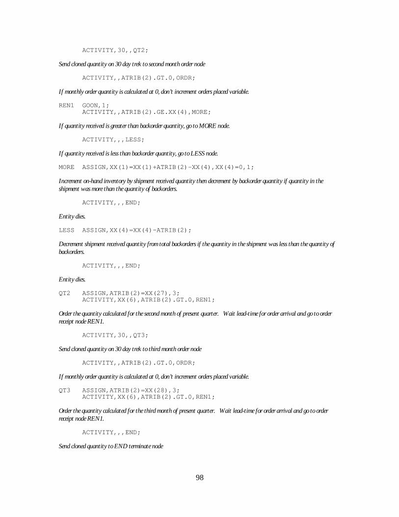
98

ACTIVITY,30,,QT2;

Send cloned quantity on 30 day trek to second month order node



REN1 GOON,1; ACTIVITY,,ATRIB(2).GE.XX(4),MORE;


ACTIVITY,,,LESS;




ACTIVITY,,,END;

Entity dies.



ACTIVITY,,,END;

Entity dies.


Order the quantity calculated for the second month of present quarter. Wait lead-time for order arrival and go to orderreceipt node REN1.

ACTIVITY,30,,QT3;

Send cloned quantity on 30 day trek to third month order node




Order the quantity calculated for the third month of present quarter. Wait lead-time for order arrival and go to orderreceipt node REN1.

ACTIVITY,,,END;

Send cloned quantity to END terminate node

99



ORDR ASSIGN,XX(21)=XX(21)+1; ACTIVITY,,,END;

Increment cumulative order quantity. Entity dies.

;

V. Annual Computation of TVC and Daily Average Backorders.;YEAR CREATE,364,364,,,1; ACTIVITY; ASSIGN,XX(35)=XX(21)*5.2,XX(23)=XX(23)/365,XX(33)=XX(23), XX(24)=XX(35)+XX(36),XX(21)=0,XX(36)=0,XX(23)=0; ACTIVITY;

Compute ordering cost and daily on hand inventory, and TVC, clearing of annual variables.

CTVC COLCT,XX(24),TVC,,1; total variable cost statistics ACTIVITY;CINV COLCT,XX(33),INV,,1; average inv

Collect TVC and average inventory.

ACTIVITY;DONE TERMINATE;

Terminate node.

; END;FIN

100

Appendix N. Periodic Order Quantity FORTRAN Subroutine


of the model as to its purpose and function.

PROGRAM MAIN DIMENSION NSET(1000000) PARAMETER (MEQT=100,MSCND=25,MENTR=25,MRSC=75,MARR=60, 1 MGAT=25,MHIST=60,MCELS=500,MCLCT=60,MSTAT=60,MEQV=100, 2 MATRB=100,MFILS=100,MPLOT=10,MVARP=10,MSTRM=10, 3 MACT=100,MNODE=500,MITYP=60,MMXXV=100,MMXFLD=100) PARAMETER(MVARP1=MVARP+1) COMMON/SCOM1/ATRIB(MATRB),DD(MEQT),DDL(MEQT),DTNOW,II,MFA, 1 MSTOP,NCLNR,NCRDR,NPRNT,NNRUN,NNSET,NTAPE,SS(MEQT), 2 SSL(MEQT),TNEXT,TNOW,XX(MMXXV) COMMON QSET(1000000) EQUIVALENCE (NSET(1),QSET(1)) NNSET=1000000 NCRDR=5 NPRNT=6 NTAPE=7 CALL SLAM STOP ENDC FUNCTION USERF(IFN) PARAMETER(MEQT=100,MSCND=25,MENTR=25,RSC=75,MARR=60, 1 MGAT=25,MHIST=60,MCELS=500,MCLCT=60,MSTAT=60,MEQV=100, 2 MATRB=100,MFILS=100,MPLOT=10,MVARP=10,MSTRM=10, 3 MACT=100,MNODE=500,MITYP=60,MMXXV=100,MMXFLD=100) PARAMETER (MVARP1=MVARP+1) COMMON/SCOM1/ATRIB(MATRB),DD(MEQT),DDL(MEQT),DTNOW,II,MFA, 1 MSTOP,NCLNR,NCRDR,NPRNT,NNRUN,NNSET,NTAPE,SS(MEQT), 2 SSL(MEQT),TNEXT,TNOW,XX(MMXXV) GOTO (10,20,30,40),IFNCC 10 I=XX(8)*XX(6) USERF=I GOTO 50 20 IF (XX(70).EQ.0) GOTO 35 R=SQRT(((2)*(5.2))/(XX(70)*XX(15)*.025)) XX(72)=R J=INT(R+.5) USERF=J GOTO 30

Calculation of Periodic Order Quantity decision variable.C

Calculation of Monthly Order Quantity 30 IF (XX(71).EQ.1) GOTO 36 GOTO 31 31 IF (XX(71).EQ.2) GOTO 37 GOTO 32 32 IF (XX(71).EQ.3) GOTO 38 35 XX(26)=0

101

XX(27)=0 XX(28)=0 GOTO 39 36 XX(26)=XX(70) XX(27)=XX(70) XX(28)=XX(70) XX(26)=INT(XX(26)+.5) XX(27)=INT(XX(27)+.5) XX(28)=INT(XX(28)+.5) GOTO 39

Order one month’s worth of inventory each month of the quarter. Round up and truncate order quantities.

37 XX(26)=(2*XX(70)) XX(27)=0.0 XX(28)=XX(70) XX(26)=INT(XX(26)+.5) XX(27)=INT(XX(27)+.5) XX(28)=INT(XX(28)+.5) GOTO 39

Order 2 month’s worth of inventory the first month and one month’s worth the third month..

38 XX(26)=(3*XX(70)) XX(27)=0.0 XX(28)=0.0 XX(26)=INT(XX(26)+.5) XX(27)=INT(XX(27)+.5) XX(28)=INT(XX(28)+.5) GOTO 39

Order 3 month’s worth of inventory the first month.

39 USERF=1 40 IF (XX(23).LE.0) GOTO 41 GOTO 49 41 XX(23)=0 49 USERF=1 50 RETURN

Return to SLAM model.

END

End FORTRAN subroutine.

102

Appendix O. Verification of the Silver-Meal Model

To verify the Silver-Meal model, mean values for each SMCC’s TBO and QPD

were inserted into the respective create nodes of the computer model. The performance

of the computer model was verified by running the models for one year and collecting

the total relevant cost (TRUC) calculations every quarter. This output was compared to

results that were calculated analytically. Model verification was completed when

computer output based on the mean input agreed with first-year analytical results. The

analytic calculations and simulation output for the TRUC of SMCC 5 are presented

below (for this SMCC, TBO was 51 days and QPD was 7 units):

Variables Used to Validate the Silver-Meal ModelVariable Description

XX(5) Actual Demand (current quarter)XX(14) Forecasted Demand (next quarter)XX(15) Unit price (v)XX(26) Silver Meal order quantity - 1st month of quarterXX(27) Silver Meal order quantity - 2nd month of quarterXX(28) Silver Meal order quantity - 3rd month of quarterXX(51) Silver Meal TRUC costs - Month 1XX(52) Silver Meal TRUC costs - Month 2XX(53) Silver Meal TRUC costs - Month 3

A Ordering costr Annual holding cost

Sequential Steps to Calculate TRUCStep Calculation

1 XX(51) = A/12 XX(52) = [A + ((XX(14)/3) * (1) * XX(15) * r/12)]/23 XX(53) = [(A + ((XX(14)/3) * (1) * XX(15) * r/12)) + ((XX(14)/3) * (2) * XX(15) * r/12)]/3

103

1. Validation of Quarter One (SMCC 5)

TRUC Calculation (Qtr 1)Step Variable Result

1 XX(51) 5.20/1 = 5.202 XX(52) [5.20 + ((7/3) * (1) * 1409 * 0.10/12)]/2 = 16.2993 XX(53) [(5.20 + ((7/3) * (1) *1409 * 0.10/12)) + ((7/3) * (2) * 1409 * 0.10/12)]/3 = 29.131

Note: XX(51) < XX(52) < XX(53). Place order every month during the quarter. Orderquantity is 7/3 or 2.33 units. When rounded, this order quantity is 2 units per month.

Computer Simulation Output (Qtr 1)S L A M I I S U M M A R Y R E P O R T**STATISTICS FOR TIME-PERSISTENT VARIABLES**

MEAN STANDARD MINIMUM MAXIMUM CURRENT VALUE DEVIATION VALUE VALUE VALUEXX5 ACTUAL 0.1538E+01 0.2899E+01 0.0000E+00 0.7000E+01 0.7000E+01XX14QFD 0.5731E+01 0.4784E+01 0.0000E+00 0.1400E+02 0.1400E+02XX26QT1 VALUE 0.2000E+01 0.0000E+00 0.0000E+00 0.2000E+01 0.2000E+01XX27QT2 VALUE 0.2000E+01 0.0000E+00 0.0000E+00 0.2000E+01 0.2000E+01XX28QT3 VALUE 0.2000E+01 0.0000E+00 0.0000E+00 0.2000E+01 0.2000E+01XX51SMT1 0.5200E+01 0.0000E+00 0.0000E+00 0.5200E+01 0.5200E+01XX52SMT2 0.1630E+02 0.0000E+00 0.0000E+00 0.1630E+02 0.1630E+02XX53SMT3 0.2913E+02 0.9537E-06 0.0000E+00 0.2913E+02 0.2913E+02

2. Validation of Quarter Two (SMCC 5)


1 XX(51) 5.20/1 = 5.202 XX(52) [5.20 + ((14/3) * (1) * 1409 * 0.10/12)]/2 = 29.9973 XX(53) [(5.20 + ((14/3) * (1) *1409* 0.10/12)) + ((14/3) * (2) * 1409 * 0.10/12)]/3 = 56.528



MEAN STANDARD MINIMUM MAXIMUM CURRENT VALUE DEVIATION VALUE VALUE VALUEXX5 ACTUAL 0.3821E+01 0.4749E+01 0.0000E+00 0.1400E+02 0.1400E+02XX14QFD 0.6051E+01 0.4755E+01 0.0000E+00 0.1400E+02 0.1400E+02XX26QT1 VALUE 0.3000E+01 0.1414E+01 0.0000E+00 0.5000E+01 0.5000E+01XX27QT2 VALUE 0.3000E+01 0.1414E+01 0.0000E+00 0.5000E+01 0.5000E+01XX28QT3 VALUE 0.3000E+01 0.1414E+01 0.0000E+00 0.5000E+01 0.5000E+01XX51SMT1 0.5200E+01 0.0000E+00 0.0000E+00 0.5200E+01 0.5200E+01XX52SMT2 0.2086E+02 0.6458E+01 0.0000E+00 0.3000E+02 0.3000E+02XX53SMT3 0.3826E+02 0.1292E+02 0.0000E+00 0.5653E+02 0.5653E+02

104

3. Validation of Quarter Three (SMCC 5)


1 XX(51) 5.20/1 = 5.202 XX(52) [5.20 + ((14/3) * (1) * 1409 * 0.10/12)]/2 = 29.9973 XX(53) [(5.20 + ((14/3) * (1) *1409* 0.10/12)) + ((14/3) * (2) * 1409 * 0.10/12)]/3 = 56.528




4. Validation of Quarter Four (SMCC 5)


1 XX(51) 5.20/1 = 5.202 XX(52) [5.20 + ((14/3) * (1) * 1409 * 0.10/12)]/2 = 29.9973 XX(53) [(5.20 + ((14/3) * (1) *1409* 0.10/12)) + ((14/3) * (2) * 1409 * 0.10/12)]/3 = 56.528




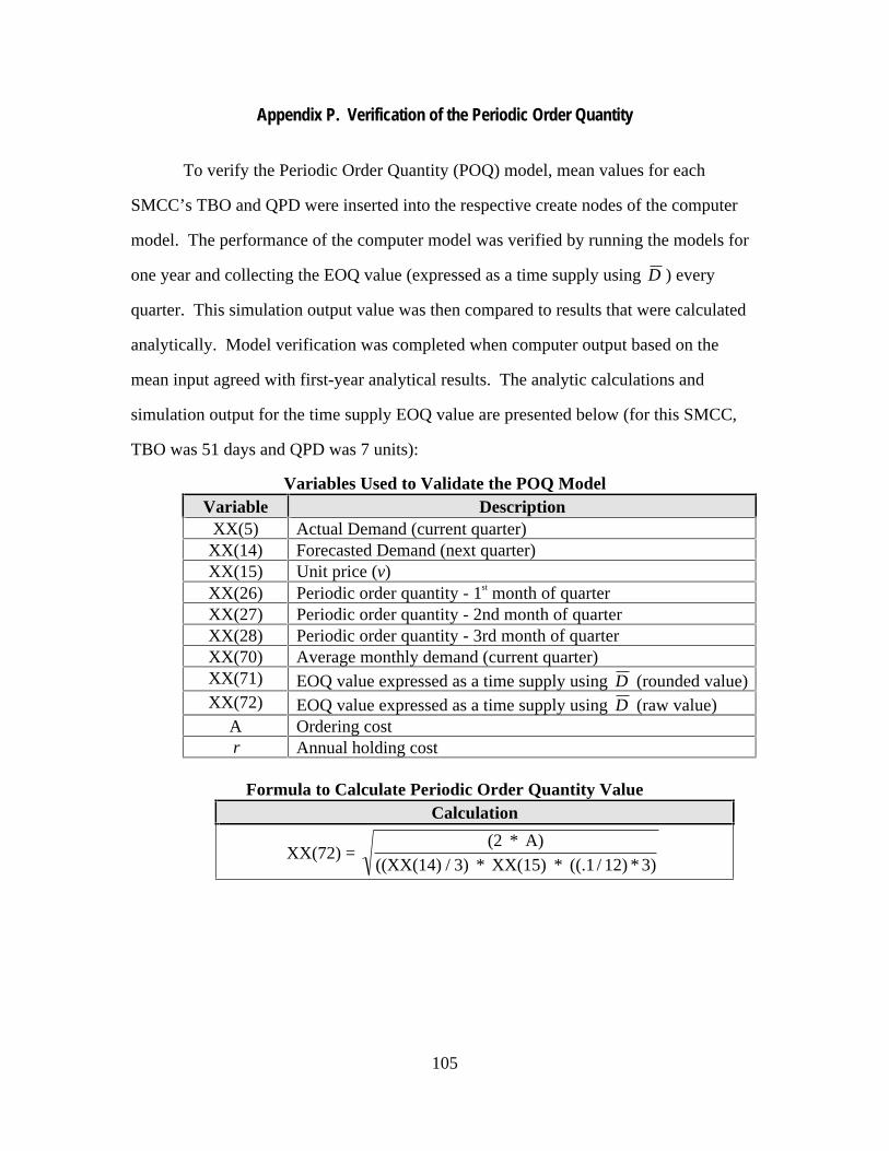
105

Appendix P. Verification of the Periodic Order Quantity

To verify the Periodic Order Quantity (POQ) model, mean values for each

SMCC’s TBO and QPD were inserted into the respective create nodes of the computer

model. The performance of the computer model was verified by running the models for

one year and collecting the EOQ value (expressed as a time supply using D ) every

quarter. This simulation output value was then compared to results that were calculated

analytically. Model verification was completed when computer output based on the

mean input agreed with first-year analytical results. The analytic calculations and

simulation output for the time supply EOQ value are presented below (for this SMCC,

TBO was 51 days and QPD was 7 units):

Variables Used to Validate the POQ ModelVariable Description

XX(5) Actual Demand (current quarter)XX(14) Forecasted Demand (next quarter)XX(15) Unit price (v)XX(26) Periodic order quantity - 1st month of quarterXX(27) Periodic order quantity - 2nd month of quarterXX(28) Periodic order quantity - 3rd month of quarterXX(70) Average monthly demand (current quarter)XX(71) EOQ value expressed as a time supply using D (rounded value)XX(72) EOQ value expressed as a time supply using D (raw value)


Formula to Calculate Periodic Order Quantity ValueCalculation

XX(72) = (2 * A)

((XX(14) / 3) * XX(15) * ((.1 / 12) * 3)

106


POQ Calculation (Qtr 1)Calculation

XX(72) = (2 * 5.2)

((XX(7) / 3) * XX(15) * ((.1 / 12) * 3) = 0.35571

Note: XX(72) is rounded up to 1. Place an order every month during the quarter. Orderquantity is 7/3 or 2.33 units. When rounded, this order quantity is 2 units per month.


MEAN STANDARD MINIMUM MAXIMUM CURRENT VALUE DEVIATION VALUE VALUE VALUEXX5 ACTUAL 0.1538E+01 0.2899E+01 0.0000E+00 0.7000E+01 0.7000E+01XX14FCSTDMD 0.5731E+01 0.4784E+01 0.0000E+00 0.1400E+02 0.1400E+02XX26QT1 VALUE 0.1000E+01 0.1000E+01 0.0000E+00 0.2000E+01 0.2000E+01XX27QT2 VALUE 0.1000E+01 0.1000E+01 0.0000E+00 0.2000E+01 0.2000E+01XX28QT3 VALUE 0.1000E+01 0.1000E+01 0.0000E+00 0.2000E+01 0.2000E+01XX70 0.2333E+01 0.0000E+00 0.0000E+00 0.2333E+01 0.2333E+01XX71PERIOD 0.1000E+01 0.0000E+00 0.0000E+00 0.1000E+01 0.1000E+01XX72VALUE 0.3557E+00 0.0000E+00 0.0000E+00 0.3557E+00 0.3557E+00



XX(72) = (2 * 5.2)

((14 / 3) * 1409 * ((.1 / 12) *3) = 0.25152



MEAN STANDARD MINIMUM MAXIMUM CURRENT VALUE DEVIATION VALUE VALUE VALUEXX5 ACTUAL 0.3821E+01 0.4749E+01 0.0000E+00 0.1400E+02 0.1400E+02XX14FCSTDMD 0.6051E+01 0.4755E+01 0.0000E+00 0.1400E+02 0.1400E+02XX26QT1 VALUE 0.2333E+01 0.2055E+01 0.0000E+00 0.5000E+01 0.5000E+01XX27QT2 VALUE 0.2333E+01 0.2055E+01 0.0000E+00 0.5000E+01 0.5000E+01XX28QT3 VALUE 0.2333E+01 0.2055E+01 0.0000E+00 0.5000E+01 0.5000E+01XX70 0.3111E+01 0.1100E+01 0.0000E+00 0.4667E+01 0.4667E+01XX71PERIOD 0.1000E+01 0.0000E+00 0.0000E+00 0.1000E+01 0.1000E+01XX72VALUE 0.3210E+00 0.4911E-01 0.0000E+00 0.3557E+00 0.2515E+00

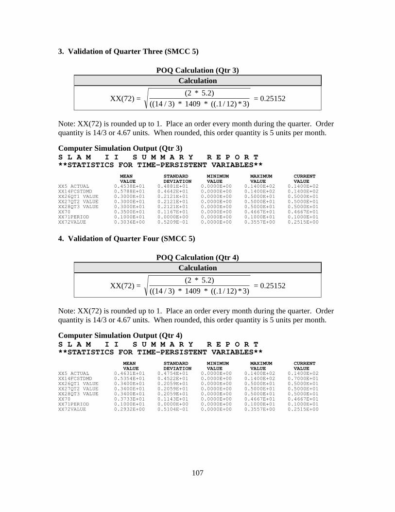
107



XX(72) = (2 * 5.2)

((14 / 3) * 1409 * ((.1 / 12) *3) = 0.25152




4. Validation of Quarter Four (SMCC 5)


XX(72) = (2 * 5.2)

((14 / 3) * 1409 * ((.1 / 12) *3) = 0.25152




108

Appendix Q. Verification of the DLA Economic Order Quantity Model

To verify the DLA Economic Order Quantity (EOQ) model, mean values for

each SMCC’s TBO and QPD were inserted into the respective create nodes of the

computer model. The performance of the computer model was verified by running the

models for one year and collecting the EOQ value every quarter. This simulation output

value was then compared to results that were calculated analytically. Model verification

was completed when computer output based on the mean input agreed with first-year

analytical results. The analytic calculations and simulation output for the EOQ value are

presented below (for this SMCC, TBO was 51 days and QPD was 7 units):

Variables Used to Validate the EOQ ModelVariable Description

XX(5) Actual Demand (current quarter)XX(7) EOQ ValueXX(14) Forecasted Demand (next quarter)XX(15) Unit price (v)


Formula to Calculate Economic Order Quantity ValueCalculation

XX(7) = (2 * A * (XX(5))

* ((v r / )12) * 3

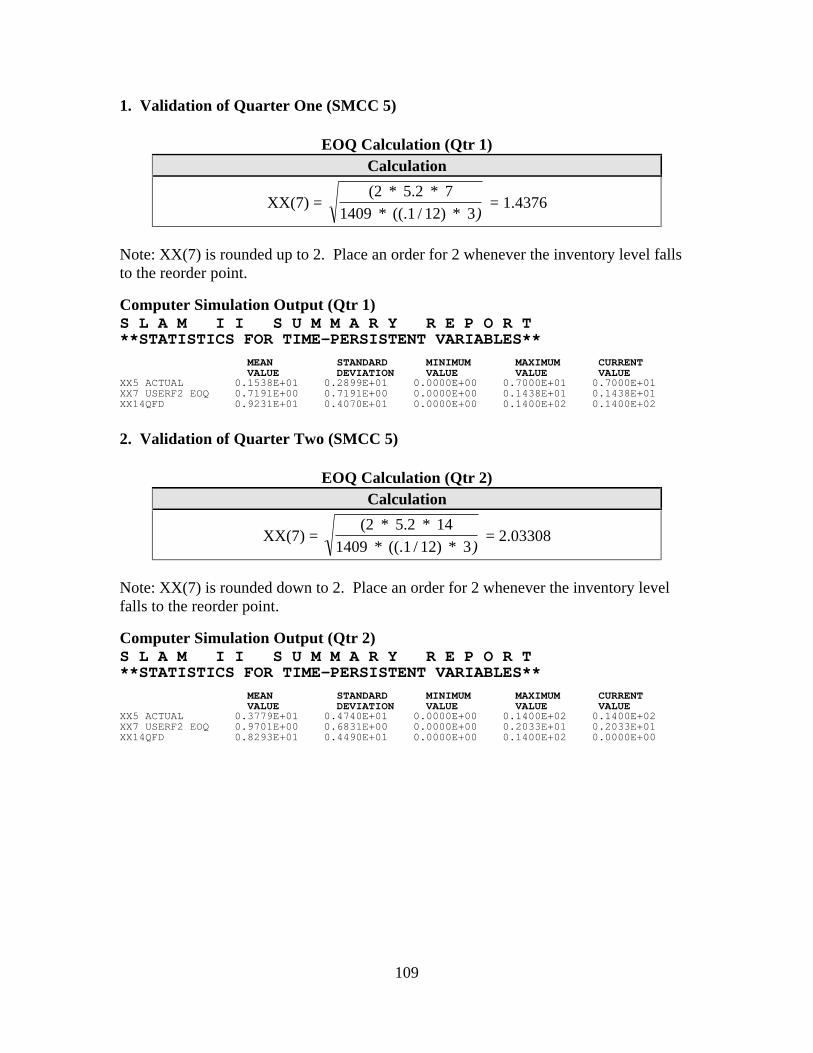
109


EOQ Calculation (Qtr 1)Calculation

XX(7) = (2 * 5.2 * 7

1409 * ((.1 / 12) * 3) = 1.4376

Note: XX(7) is rounded up to 2. Place an order for 2 whenever the inventory level fallsto the reorder point.


MEAN STANDARD MINIMUM MAXIMUM CURRENT VALUE DEVIATION VALUE VALUE VALUEXX5 ACTUAL 0.1538E+01 0.2899E+01 0.0000E+00 0.7000E+01 0.7000E+01XX7 USERF2 EOQ 0.7191E+00 0.7191E+00 0.0000E+00 0.1438E+01 0.1438E+01XX14QFD 0.9231E+01 0.4070E+01 0.0000E+00 0.1400E+02 0.1400E+02



XX(7) = (2 * 5.2 * 14

1409 * ((.1 / 12) * 3) = 2.03308

Note: XX(7) is rounded down to 2. Place an order for 2 whenever the inventory levelfalls to the reorder point.



110



XX(7) = (2 * 5.2 * 14

1409 * ((.1 / 12) * 3) = 2.03308






XX(7) = (2 * 5.2 * 14

1409 * ((.1 / 12) * 3) = 2.03308




111

References

Ahadiat, Nasrollah. “Solving Inventory Problems by Simulation,” Journal of Systems Management: 29-35 (September, 1986).

Ammer, Dean S. Materials Management and Purchasing. Homewood IL: Richard D. Irwin, Inc., 1980.

Barrett, D. A. Automatic Inventory Control Techniques. London: Business Books Ltd., 1969.

Berry, Harry A. and Edward E. Tatge. An Evaluation of the Appropriateness of theDefense Logistics Agency’s Requirements Model. MS thesis,AFIT/GIM/LAL/95S-1. Graduate School of Logistics and AcquisitionManagement, Air Force Institute of Technology (AU), Wright-Patterson AFBOH, September 1995 (AD-A300454).

Bilikam, Robert. Operation Research Analysis and Projects Division, Defense Supply Center Columbus (West) (DSCC/EIR), Dayton OH. Personal Interview.23 February 1996.

DLA Fact Sheet. Facts About The Defense Logistics Agency. Defense LogisticsAgency, 1996.

DLA Pamphlet. The ABCs of DLA. Washington: Government Printing Office, 1992.

Dopuch, Nicholas, Jacob Birnberg, and Joel Demski. Cost Accounting, Accounting Datafor Management’s Decisions. New York: Harcourt, Brace, Javanovich, Inc., 1974.

Emory, C. William, Business Research Methods. Homewood IL: Richard D. Irwin,Inc., 1980.

Erlenkotter, Donald. “Ford Whitman Harris and the Economic Order Quantity Model,” Operations Research, 38: 937-944 (November-December 1990).

Fulbright, John E. “Advantages and Disadvantages of the EOQ Model,” Journal of Purchasing and Materials Management: 8-10 (Spring 1979).

Gay, L. R. and P. L. Diehl. Research Methods for Business and Management. New York: Macmillan Publishing Company, 1992.

Heilweil, Norman L. “Why Inventory,” in APICS Inventory Management Reprints. Unedited. Falls Church VA: American Production and Inventory Control Society, Inc., 1986.

112

Hoover, Stewart V. and Ronald F. Perry. Simulation: A Problem-Solving Approach. Reading MA: Addison-Wesley Publishing Company, 1990.

House, William C. Business Simulation for Decision Making. New York: Princeton, 1977.

Kaimann, Richard A. “E.O.Q. Revisited,” Journal of Purchasing, 5: 68-69 (May 1969).

Kleijnen, Jack P.C. Statistical Tools For Simulation Practitioners. New York: MarcelDekker, Inc., 1987.

Law, Averill M. and W. David Kelton. Simulation Modeling and Analysis. NewYork: McGraw-Hill, Inc., 1991.

Long, William S. and Douglas H. Engberson. The Effect of Violations of the ConstantDemand Assumption on the Defense Logistics Agency Requirements Model. MSthesis, AFIT/GLM/LAL/94S-15. Graduate School of Logistics and AcquisitionManagement, Air Force Institute of Technology (AU), Wright-Patterson AFBOH, September 1994 (AD-A285272).

Love, Stephen F. Inventory Control. New York: McGraw-Hill, Inc., 1979.

Magad, Eugene L. and John M. Amos. Total Materials Management: The Frontier for Maximizing Profit in the 1990s. New York: Van Nostrand Reinhold, 1989.

McClave, James T. and P. George Benson. Statistics For Business and Economics, 6th Ed. New York: Macmillan College Publishing Company, 1994.

Osteryoung, Jerome S., Daniel E. McCarty and Walter J. Reinhart. “Use of the EOQ Model for Inventory Analysis,” Production and Inventory Management: 39-45 (Third Quarter 1986).

Peckham, Herbert H. Effective Materials Management. Englewood Cliffs: Prentice-Hall, Inc., 1972.

Perry, James H. “Reconciling Procurement and Inventory Management Objectives in Department of Defense Spares Acquisition,” National Contract Management Journal, 24: 1-6 (Issue 1 1991).

Petrovic, R., A. Senborn, and M. Vujosevic. Hierarchical Spare Parts InventorySystems. New York: Elsevier Science Publishing, Inc., 1986.

Philippakis, Andreas S. “The Cost of Using EOQ With Variable Demand Items,”Journal of Purchasing, 6: 66-71 (November 1970).

113

Plossl, G. W. and O. W. Wight. Production and Inventory Control. Englewood Cliffs: Prentice-Hall, Inc., 1967.

Robinson, Nathaniel. The Defense Logistics Agency, Providing Logistics Support Throughout the Department of Defense. Research Report No. AU-ARI-92-4.Maxwell Air Force Base AL. Air University Press, October 1993.

Sekaran, Uma. Research Methods for Business. New York: John Wiley & Sons, Inc., 1992.

Silver, Edward A. “A Simple Inventory Replenishment Decision Rule for a LinearTrend in Demand,” Journal of the Operational Research Society, 30: 71-75 (Number 1

1979).

Silver, Edward A. and Harlan C. Meal. “A Heuristic for Selecting Lot Size Quantitiesfor the Case of Deterministic Time-Varying Demand Rate and Discrete Opportunities

for Replenishment,” Production and Inventory Management, 14: 64-74 (Second Quarter 1973).

Silver, Edward A. and Rein Peterson. Decision Systems for Inventory Management and Production Planning. New York: John Wiley & Sons, 1985.

Starr, Martin K. and David W. Miller. inventory control: theory and practice.Englewood Cliffs: Prentice-Hall, Inc., 1962.

Tersine, Richard. Principles of Inventory and Materials Management. New York: Elsevier Science Publishing, Inc., 1982.

Tersine, Richard J. and John H. Campbell. Modern Materiels Management. New York: Elsevier Science Publishing, Inc., 1977.

Wagner, Harvey M. Principles of Management Science. Englewood Cliffs: Prentice-Hall, Inc., 1970.

Waters, C. D. J. Inventory Control and Management. New York: John Wiley & Sons, 1992.

114

Goulet Vita

Captain Wayne C. Goulet was born on 2 February 1964 in Marlboro,

Massachusetts. He attended St. John’s High School in Shrewsbury, Massachusetts,

graduating in 1982. He enlisted in the Air Force in 1986 as a supply technician. In 1989

he graduated from Nova Southeastern University with a Bachelor of Science degree in

Professional Management. In 1991 he graduated from Officer’s Training School with a

commission as a second lieutenant.

Captain Goulet was formerly stationed at Howard AFB, Panama and McClellan

AFB, Sacramento CA. His last assignment was at the 89th Supply Squadron, Andrews

AFB, MD where he served as the Fuels Management Officer. Captain Goulet entered the

Graduate School of Logistics and Acquisition Management in May 1995 and graduated

in September of 1996. He received a follow-on assignment to the 633 Air Mobility

Support Squadron, Kadena AB, Japan.

He and his wife Bethsabet have two sons, Israel, age 12, and Charlie, age 5.

Permanent Address:31 Simpson RoadMarlboro, MA 01752

115

Rollman Vita

First Lieutenant Michael L. Rollman was born on 10 December 1960 in Topeka,

Kansas. He attended Oak Ridge High School in Orlando, Florida, graduating in 1979.

He enlisted in the Air Force in 1979 as a supply technician. In 1992 he graduated from

the University of Maryland with a Bachelor of Science degree in Business

Administration. In 1993 he graduated from Officer’s Training School with a

commission as a second lieutenant.

Lieutenant Rollman was formerly stationed at Hancock Field, NY, Osan AB,

Korea, Lowry AFB, CO, Misawa AB, Japan, Kadena AB, Japan, and Fort Riley Army

Post, KS. His most recent assignment was to the 47th Logistics Squadron, Laughlin

AFB, TX where he served as the Materiel Management Officer. Lieutenant Rollman was

selected to attend the Air Force’s Graduate School of Logistics and Acquisition

Management in May 1995 and graduated in September of 1996 with a Masters Degree in

Logistics Management. He received a follow-on assignment to the 626th Air Mobility

Support Squadron, Rhein-Main AB, Germany.

He and his wife Suk Cha have two daughters, Heather, age 9, and Sarah, age 7.

Permanent Address:73 Meehan DriveDayton, OH 45431

afit/gtm/lal/96s-6 · afit/gtm/lal/96s-6 a study of defense ... advantages of the eoq ......

Documents