WORKING PAPER SERIES

Age Distributions and Returns of Financial Assets

Peter S. Yoo

Working Paper 1994-002A

http://research.stlouisfed.org/wp/1994/94-002.pdf

FEDERAL RESERVE BANK OF ST. LOUISResearch Division

411 Locust Street

St. Louis, MO 63102

______________________________________________________________________________________

The views expressed are those of the individual authors and do not necessarily reflect official positions of

the Federal Reserve Bank of St. Louis, the Federal Reserve System, or the Board of Governors.

Federal Reserve Bank of St. Louis Working Papers are preliminary materials circulated to stimulate

discussion and critical comment. References in publications to Federal Reserve Bank of St. Louis Working

Papers (other than an acknowledgment that the writer has had access to unpublished material) should be

cleared with the author or authors.

Photo courtesy of The Gateway Arch, St. Louis, MO. www.gatewayarch.com

AGE DISTRIBUTIONS AND RETURNS OF FINANCIAL ASSETS

February 1994

ABSTRACT

This paper explores the relationship between age distribution and asset returns impled by an

overlapping-generations asset pricing model. The model predicts that as more individuals reach the age when

the increment to their wealth reaches its maximum, asset returns fall.

Cross-sectional evidence from the Survey of Financial Characteristics of Consumers and the Surveys of

Consumer Finances indicates that individuals aged 45 to 54 have the largest increment to wealth of all age

group. Time series estimates confirm that a close link exists between aggregate household wealth and the size

of this age group. In accordance with the model presented in this paper, time series estimates of the

relationship between asset returns and age distribution suggests a large, statistically significant, negative

correlation between the fraction of the population aged 45 to 54 and the returns of several types of assets.

KEYWORDS: Asset pricing, demographics

JEL CLASSIFICATION: D91, E44, Gl2, Jil

Peter S. YooEconomistFederal Reserve Bank of St. Louis411 Locust StreetSt. Louis, MO 63102

I would like to thank Ben Friedman, Greg Mankiw, Mike Pakko, Joe Ritter, Steve Schran, Jon Skinner, JimThomson, David Weil and Philippe Weil for their helpful comments and suggestions. Rich Taylor providedexcellent research Assistance. All remaining errors are mine.

I. Introduction

Two recent papers have focused on the population’s age distribution asa possible source of low frequency movement in asset prices. Mankiw andWeil [1989] posit that the demand for housing and the growth of the adultpopulation are correlated. The maturing of the baby boomers during the1970’s accelerated the rate of household formation, which in turn, increasedthe demand for housing and thus, increased the real price of housing. Con-sistent with their hypothesis, they find a positive relationship between therate of household formation and the real price of housingduring the post-warera. Bakshi and Chen [1994] argue that as the population ages, the demandfor housing decreases while the demand for securities increases. They findthat real S&P 500 prices covary positively with the average age of the U.S.population for the post-war period.

The surprising aspect of the literature is not that such relationships ex-ist among asset prices and the population’s age distribution, but that sucha direct implication of standard models with demographic variables has re-ceivedso little attention. For example, the life-cycle hypothesis suggests thata young population has more saving than an old population. The~differencesin the supply of saving imply that the age structure of the population affectasset returns.

In this paper, I present a multiperiod, overlapping-generations asset pric-ing model that explores the relationship between an economy’s age distri-bution and asset returns. The model predicts that the relative size of theage group with the largest increment to their lifetime wealth has the largestnegative relationship with asset returns. Cross-sectional evidence from the1983 Survey of Consumer Finances indicates that individuals aged 45 to 54have the largest increment to wealth of any age group. Time series estimatesconfirm that a close link exists between aggregate household wealth and therelative size of this age group. In accordance with the model presented inthis paper, time series estimates of the relationship between asset returnsand the economy’s age distribution find a large, statistically significant, neg-ative correlation between the fraction of the population aged 45 to 54 andthe returns of several types of assets.

The paper proceeds as follows. First, I review a multiperiod overlapping-generations asset pricing model that formally describes the relationship be-tween cohort size and asset returns. I then verify the empirical validity ofthe model in three steps. I first use cross-sectional evidence from the 1983

1

Survey of Consumer Finances to estimate the empirical relationship betweenwealth and age. Next, I turn to estimates of aggregate household wealth toverify the existence and stability of the wealth-age relationship found inthe household data. Finally, I present time series estimates of the relation-ship among several types of financial asset returns and the population agedistribution.

II. A Multiperiod Asset Pricing Model

A multiperiod overlapping-generations version of the Lucas [1978] assetpricing model is an obvious way to think about the relationship between theage distribution and asset returns. Agents maximize their lifetime utilitysubject to an age dependent path of endowments. Consequently, the quan-tity of assets theychoose to hold at any given time will depend on their age.This difference in asset holdings, when aggregated, affects the size of totalhousehold wealth, and thus, induces a relationship between the population’sage distribution and the returns to assets.

A. Model

Each agent spends 7~years in childhood, retires at age Ta, and dies atage 1~.The agent also maximizes his lifetime utility subject to a lifetimebudget constraint.

max~ (1 + 5)1_S t+8—1,8 (1)s=1 ‘p

subject to the budget constraint,

(1 + rt+s_1) at+s_2,s_1 + e.~— Ct+s_1,s. (2)

ct,5

and at,5 are consumption and asset holdings of an agent s years old inperiod t. rt is the rate of return for holding an asset between periods t — 1and t. e5 is the endowment of a non-storable good received by an agent syears old. 5 is the subjective discount rate, and p is the coefficient of relativerisk aversion.

In equilibrium, aggregate consumption must equal aggregate endowment

2

every period,~’

>50t (s) e8 = ~‘Pt (s) ct,~, (3)

where S°t(s) is the age distribution of the population in period t.

Given the level of generality, no closed form solution to the above prob-lem exist but numerical solutions for the equilibrium asset prices are possible.

B. Simulation

Varying s~t(s), then solving (1) and (3) for rt determines the relationshipbetween a population’s age distribution and asset returns.2 Since the babyboom is the most prominent feature of modern U.S. demographic history,I use a stylized baby boom, a temporary doubling of the annual popula-tion growth rate from one percent to two percent for fifteen years, as aninteresting change in the population distribution, 5°t(s) .~ The simulationassumes that the start and the end of the baby boom are unexpected shocksto the population growth rate. Table 1 shows the value of the other modelparameters, which are equal to those used by Auerbach and Kotlikoff. TheendOwment pattern also corresponds to the pattern used by Auerbach andKotlikoff, with individuals 20 years old and younger, as well as those over65, receiving no endowments. I normalized the endowment pattern so thate21 =

The simulation shows that fluctuations in the population age distributionproduce changes in asset returns.5 The top panel of figure 1 shows the pathof asset returns and the fraction of the population aged 45, and it shows aclear negative relationship between the two variables. The simulation alsoindicates that the magnitude of the relationship is on the order of two, thatis a percentage point change in the relative size of the 45 year old group

‘Appendix A outlines the model with investment in productive capital, where assetreturns are then equal to the rate of return of capital.

2This is similar to Auerbach and Kotlikoff {1987].3The population growth rate nearly doubled from an annual rate of one percentduring

the period before 1947 to an annual rate near two percent for the fifteen or so years of thebaby boom. Thereafter, the growth rate returned to the previous rate, although it hasnow fallen below one percent.

4The endowment pattern has the functional forme8

= exp (4.47+ 0.033s — 0.0006782).5The simulation results from the model with productive capital is very similar to that

of the asset pricing model.

3

corresponds to a two percent point change in asset returns. The simplecorrelation between the two series is near 0.9.

Why is the relative size of 45 year old agents so important in determiningthe returns of assets? The bottom panel of figure 1 suggests that the agegroups with the largest positive increment to wealth should have the largestnegative correlation with asset returns. It shows two plots: the correlationsamong asset returns and the relative sizes of the endowment receiving agegroups, and the changes in wealth for each age s, L~~at,5= at,5 — at_i,3_i.The correlations reach a maximum, in absolute value, at 45, the age withthe largest increment to wealth. Intuitively, this is very appealing. Therelative supply and demand for saving determines the rate of returns forassets. So, the age group that has the largest positive increment to wealthhas the largest positive impact on the relative supply of saving, and thus,has the largest negative relationship with asset returns.

The results of this model adds the understanding of the effects of de-mographic variables on assets considered by Mankiw and Weil, and Bakshiand Chen. The model suggests that a population’s age structure affects amuch wider class of assets than housing. It also suggests that a population’saverage age does not fully capture the age dependence of asset prices. Sothe results of this paper’s model is consistent with the behavior of assetprices after 1945, the period studied by Bakshi and Chen, but eventually,the two models predict different paths of asset prices as the baby boomerscontinue to age dueto the nonlinear effect of a baby boom in my model. Themodel, however, makes no predictions about any differences in the responseof various assets to changes in the demographic composition of the popula-tion, whereas Bakshi and Chen predict changes in the equity premium asthe population ages. This is most likely due to the assumption of absoluterisk aversion by Bakshi and Chen.

III. The Empirical Relationship

Given the simulation results above, I now turn to the empirical veri-fication of the simulation’s results in three steps. First, I examine cross-sectional evidence from a household survey to determine the wealth ageprofile of households, indentifying the age group with the largest incrementto wealth. Next, I check the stability of the cross-sectional finding by deter-mining the age group with the largest correlation with aggregate householdwealth. Finally, I estimate time-series regressions to see if asset returns and

4

age distribution are related in the manner predicted by the model.

A. Cross-Sectional Estimates

The model suggests that the age groups with the largest increment towealth should have the largest negative correlation with asset returns. I,therefore, use the 1983 Survey of Consumer Finances to determine whichage group has the largest increment to wealth.6

To determine the wealth-age relationship, I estimate cross-sectional re-gressions using gross assets and net worth as measures of wealth.7 The re-gressions control for income and other household characteristicswith dummyvariables for the five age groups, 25-34, 35-44, 45-54, 55-64 and 65+. I usethese age groups because they correspond to the aggregate time series dataused in the next two sections. The estimated regression is

wealthj = ao + aiage: 25-341 + a~age: 35-441

+a3 age: 45-54~+ a~iage: SS-64j + a~age: 65t+a6 # of children1 + ~ # of adults + a~# of retired1 (4)+ag gender1 + alo raced + all marriedj + a12 high school1

+a13 college1 + a14 # working1 +a~ total incorne~

Table 2 presents the estimated coefficients of the dummy variables for thedifferent age groups from cross-sectional regressions (4) using the 1983 Sur-vey of Consumer Finances.8 The regressions suggest that the ages between45 and 54 represent a turning point in a household’s pattern of accumulatedwealth and indebtedness. The change in wealth is nearly $80,000, goingfrom a value of a2 = —39 to a3 = 41, a large change in gross and net wealthbetween households aged 35 to 44, and those aged 45 to 54~9The F-statistics

6See Avery, et al, f1984a, 19Mb and 1986] for some discussion about the survey.7Gross assets include: checking accounts, money market accounts, savings accounts,

IRAs, CDs, savings bonds, bonds, stocks, mutual funds, trust accounts, cash value ofwhole life insurance, loans owed to househo’-4, gas leases, gross value of land contracts,current value of home, and gross value of other properties. Net wealth equals gross assetsless total debt.

8Estimating the cross-sectional regressions without the demographic factors correlatedwith age, as in Mankiw and Well, does not change the basic relationship illustrated intable 2. In fact the pattern observed in table 2 becomes even morepronounced, indicatingthat the increase in the wealth of households aged 45 to 54 is even greater than indicated.

9The increase in wealth need not arise from achange in thesaving rate of an individual.An increase in labor income, which according to estimates from household surveys, reachesits peak between the ages of 45 and 54, will also increase the wealth of a household. Usingaggregate quarterly data between 1954:1 and 1988:4, Fair and Dominguez [1991] fInd thatconsumption relative to disposable income reaches its minimum near the age of forty years.

5

shown in table 2 are for the hypothesis that the dummy variables for thefive age groups do not covary with wealth or debt, and in all three cases,the evidence rejects the hypothesis that the coefficients for the age dummiesare insignificant at the one percent significance level.

From the estimates of the wealth-age profile it appears that individualsaged 45 to 54 have the largest increase in accumulated wealth of all agegroups. While older groups may continue to save, the incremental changesin wealth are not as large as the increase observed among the ages 45 to

This result is appealing on an intuitive level. Younger households haverelatively low labor income and high expenditures associated with buyinghouses and raising and educating their children. Between the ages of 45 and54 most households’ children have completed their schooling and left home.Furthermore, households in this age group are reducing their indebtednessfrom mortgages and other loans, and are enjoying peak labor income.11

B. Aggregate Wealth-Age Relationship

The cross-sectional regressions identify the age between 45 and 54 asthe age when wealth accumulation occurs most rapidly. This implies anexistence of a strong positive relationship between the relative size of theage group 45 to 54 and the size of aggregate household wealth, providedaggregation does not distort the relationship between age and wealth, and

‘°Andoand Kennickell [1987] suggest that a sample selection bias may exist in estimatesof household wealth of retired individuals when the sample comes from household surveysbecause the surveys include only those retired households with sufficient means to supportthemselves during retirement. Those unable to support themselves are most likely livingwith their children or in nursing homes. If Ando and Kennickell’s suggestion is true, themeans and cross-sectional regression estimated overstate the wealth of the post-retirementindividuals.

Shono+s [1975] suggests that wealthy individuals have longer life expectancies. There-fore estimates based on individuals may overstate the wealth of the representative agent.

Bosworth, et al. [1991] and other studies based on household surveys indicate little or nocorrelation between the life-cycle stage of a household and its saving rate. Studies basedon aggregate data suggest that private saving rates increase as the population reachesretirement ageand decreases after retirement. Well [1992] offers a possible solution to thisdiscrepancy. He suggests that household data do not reflect the dissaving of the retireesbecause the data fails to capture the anticipatory spending of bequests by the youngergeneration. Accounting for bequests appears to minimize the discrepancy.

“The survey indicates that peak household income occurs between the ages of 45 and54.

6

the relationship is relatively stable over time.

To test this implication, I use estimates of aggregate household wealthfor the years 1946 to 1988 from the Federal Reserve’s Balance Sheets forthe U.S. Economy: 19~9to 1990. The publication contains estimates ofaggregate household wealth — gross assets, net wealth, and net purchases ofequities — which I converted into 1982 dollars and in per capita terms. Grossassets include deposits and credit market instruments, corporate equities, lifeinsurance, and few other financial assets, as well as reproducible assets andland. Net wealth subtracts total liabilities from gross assets. I detrendedthe two measures of aggregate wealth by estimating a log-linear regression ofthe respective measures of aggregate wealth against a time trend. I then usethe residuals from these regressions as the dependent variables of the time-series regression linking aggregate household wealth and the age distributionof the U.S.

The Historical Statistics of the United States and various issues of theCurrent Population Reports: Population Estimates and Projections, seriesP-25 publishes the sizes of the different age groups for the years 1926 to1988. I convert the size of each age group into its fractional size of thepopulation before estimation.

Figure 2 shows a clear relationship between the fraction of the populationaged 45 to 54 and the net household purchases of equities, a simple measureof ademographic induced change in household wealth.12 Since the incrementto an individual’s wealth reaches its maximum when he is between the agesof 45 and 54, the net purchases of equities, a measure of the increases inaggregate wealth, should follow the relative size of this cohort.

Table 3 shows the results of the time-series estimates of the relationshipbetween detrended log wealth and the fraction of the population aged 25-34, 35-44, 45-54, 55-64 and 65 or older. The standard errors shown in thetable reflect the Newey-West correction for serial correlation with the laglength determined by Schwartz information criteria. The regressions revealsa large, statistically significant (at 10 percent significance level), positiverelationship between the proportion of the population aged 45 to 54 and thegrowth of the aggregate household wealth measures.

The results of the time-series estimates of the relationship among thegrowth rate of aggregate household wealth and the relative sizes of the agegroups support the pattern observed in the cross-sectional analysis. As therelative size of the population with the largest positive increment to wealth

‘2The simple correlation between the two series is 0.75.

7

increases, the growth rate of aggregate household wealth should accelerate,and indeed, the results of this section suggests that this is true.

C. Age Distributions and Asset Returns

The previous two sections imply that the 45 to 54 age group has thelargest increment to wealth, and that changes in aggregate household wealthreflect this relationship between age and wealth. I now turn to see if theempirical evidence matches the model’s prediction about the relationshipbetween the age structure of the population and asset returns.

Stocks, Bills, Bonds, and Inflation: Yearbook 1991 published by Thbot-son and Associates contains data on real annual total returns of the followingtypes of U.S. securities: common stocks, small company stocks, long-termcorporate bonds, long-term government bonds, intermediate-term govern-ment bonds and Treasury bills, for the years 1926 to 1990.’~

The following equation estimates the reduce form relationship impliedby the model:

= ~ + /3~aged: 25-34t + /32 aged: 35-44t

+/33 aged: 45-54

t + /3~aged: SS-54t + j3~aged: 65t ~ )

The simulation results suggest that the age group with the largest posi-tive increment to wealth has the largest negative correlation with asset re-turns. This result, combined with the results from the two previous sections,implies that the sign of /3~should be negative and the largest in magnitude.

I first checked the stationarity of the asset returns and the relative sizesof the age groups. In all cases, the augmented Dickey-Fuller test rejects thenull hypotheses of unit roots at the 5 percent significance level.14

Table 4 presents the regression results for the six types of financial as-sets. The t-ratios shown in the table use robust standard errors using theNewey-West correction with the Schwartz information criteria determiningthe order of the autocorrelation. The results are somewhat consistent withthe predictions of the model. In all cases, the signs of /3~are negative and inmost cases the largest in magnitude, as predicted by the model. Moreover,

‘3Total returns reinvest any dividend or interest payments made through out the yearat current price of the respective securities. Common stocks is analogous to the S&P 500,and small companies are companies with low levels of capitalization.

‘~Ifollowed the procedure outlined in Hamilton [1994], chapter 17.7 to determined thenumber of lags included in the unit root test.

8

the coefficients are often the most statistically significant. However, onlytwo of the six J33S are statistically significant.

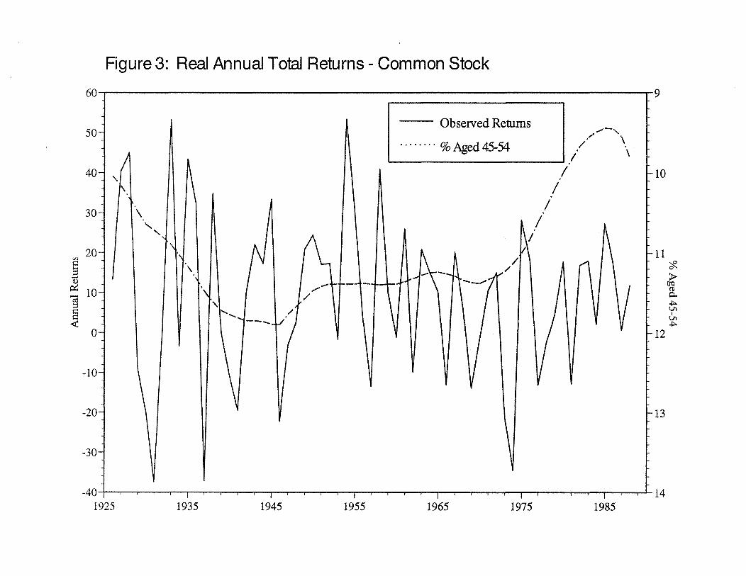
The significance of the /33s and of the regressions is inversely relatedto the volatility of the securities. Figures 3 through 8 show this clearly.They show real annual total returns of the six assets along with the fractionof the population aged 45 to 54. Note that the axes for the size of theage group are inverted. The regression for Treasury bills, the asset withthe lowest volatility, indicates that demographic factors explain nearly 50percent of the variation in the real annual returns of Treasury bill, while thedemographic factors explain none of the variation in the returns of eithertypes of stocks, the assets with the highest volatility.’5 Given the differencesin the annual volatilities between demographic variables and asset returns,this is not particularly surprising. Slow moving demographic factors willhave more of an effect on assets with low annual volatility, so that highfrequency movements are less likely to mask low frequency movements. Infact, a simple smoothing of assets returns with a three year centered movingaverage increases the adjusted B2 to 0.19, -0.02, 0A2, and 0.42 for commonstocks, small company stocks, long corporate bonds and long governmentbonds, respectively. Furthermore, such smoothing increases significance ofthe estimates shown in table 4, so that all but the coefficient for smallcompany stocks are significant at 5 percent, without noticeably altering thevalues of the point estimates.

I also estimated the regression for Treasury bills using the first differencesof the returns and demographic variables. Due to the large swings in realreturns before 1950, I smoothed the changes in real returns by taking afive year centered moving average.16 The last column of table 4 shows theresults of the regression, and it shows that the relationship found using levelsis also present in first differences. Figure 9, shows graphically the resultsof the regression. The adjusted B2 drops to 0.26 but the magnitude andthe significance of the relationship between the relative size of age groupwith the largest increment to wealth and the returns of Treasury bills areessentially unchanged.

‘5The different sizes of the relationship between age and the returns of equity andTreasury bills suggest it is possible that the equity premium may be influenced by theaging of the population, as suggested by Bakshi and Chen. The model presented in thispaper, cannot however address this issue, although using their assumption of constantabsolute risk aversion would probably induce such a result.

16~again used the Newey-West correction to calculate the standard errors, especially tocorrect the autocorrelation induced by the moving average.

9

To check the sensitivity of the regression estimates, I reestimated (5) forthe period, 1948 to 1988. Table 5 presents the results of the estimates usingthe different sample period. It suggests that demographic variables have asignificant relationship to returns of assets during the post-war era. Thesize of the coefficients are fairly robust to changes in the sample period andthe variable for the proportion of the population that is between the agesof 45 and 54 consistently maintains a sizable negative relationship with thereturns of various financial securities.

IV. Implications for Asset Returns in the United States

The results presented in this paper suggest that demographic variablesplay an important role in the determination of the low frequency movementsin the the real returns of financial assets through individual’s saving deci-sions, explaining nearly 50 percent of the variance of the annual real returnsof Treasury bills. The fact that demographic factors play a role in finan-cial markets which are usually assumed to be efficient may be surprisinggiven the predictability of the changes in the relative size of the differentage groups of the population. However if demographic factors affect thedemand for all assets in a similar manner or ifeconomic agents are liquidityconstrained or myopic, it is possible that no arbitrage opportunities exist foragents to exploit. Given the results of the paper, the entrance of the babyboomer into the 45 to 54 age group portends to a period of low real rates ofreturns, especially for Treasury bills.

The empirical portion of the paper also suggests that assets with longermaturity are less influenced by life-cycle considerations than shorter-termassets. The framework provided here sheds no light as to why this should betrue. A further examination of this difference may be an interesting avenueof research. The model would need to introduce some mechanism to induceage dependent changes in portfolio composition, like Bakshi and Chen.

10

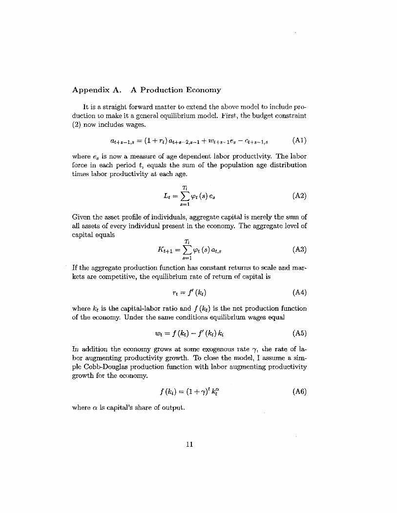
Appendix A. A Production Economy

It is a straight forward matter to extend the above model to include pro-duction to make it a general equilibrium model. First, the budget constraint(2) now includes wages.

= (1 + rt) at+s.2,s1 + wt+s_,es — ct~i,5 (Al)

where e3 is now a measure of age dependent labor productivity. The laborforce in each period t, equals the sum of the population age distributiontimes labor productivity at each age.

L~= ço~(s) e3 (A2)

Given the asset profile of individuals, aggregate capital is merely the sum ofall assets of every individual present in the economy. The aggregate level ofcapital equals

K~+,= Wt (s) at,3 (A3)

If the aggregate production function has constant returns to scale and mar-kets are competitive, the equilibrium rate of return of capital is

rt=f’(kt) (A4)

where k~is the capital-labor ratio and f (kg) is the net production functionof the economy. Under the same conditions equilibrium wages equal

wt=f(kt)—f’(kt)kt (AS)

In addition the economy grows at some exogenous rate ‘y, the rate of la-bor augmenting productivity growth. To close the model, I assume a sim-ple Cobb-Douglas production function with labor augmenting productivitygrowth for the economy.

f(kt)=(l+’y)tk~ (A6)

where ~ is capital’s share of output.

11

Table 1: Model Parameters

parameters valueT1 lifespan 80Ta retirement age 65

years of childhood 20n initial pop. growth rate 0.01c size of baby boom 0.01T duration of baby boom 155 subjective discount rate 0.015p coefficient of relative risk aversion 4

Figure 1: Simulated Relationship Between Age Distribution and Returns

rates of return (solid, right scale)

1.25 1.7

1.2 — 1.6

U)E

03 333433C 0

1.15 1.5

0.o ac~.C

a

1.1 — 1.4

1.05 1.30 10 20 30 40 50 60 70 80 90 100

% aged 45 (dotted, left scale)

4 II II liii! II III II I t II I II I II I I I I I III 111111 III

period

S433

8

0

-0.2

.04

-0.6

-0.8

—1

0.8

0.6

a

0.4 ;

a03Ca0

21 31 41 51 61

0.2

0

age

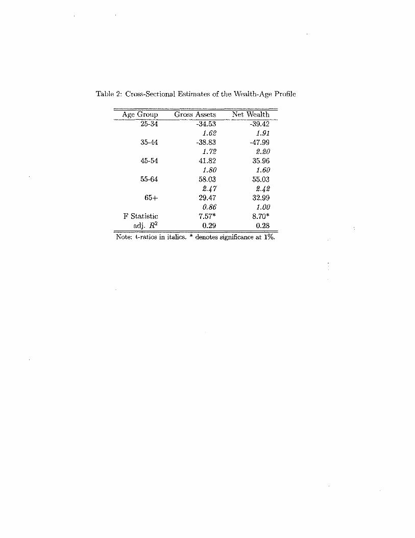
Table 2: Cross-Sectional Estimates of the Wealth-Age Profile

Age Group Gross Assets Net Wealth25-34 -34.53 -39.42

1.62 1.9135-44 -38.83 -47.99

1.72 2.2045-54 41.82 35.96

1.80 1.6055-64 58.03 55.03

2.~7 2.4265+ 29.47 32.99

0.86 1.00F Statistic 757* 8.70*

adj. B2 0.29 0.28

Note: t-ratios in italics. * denotes significance at 1%.

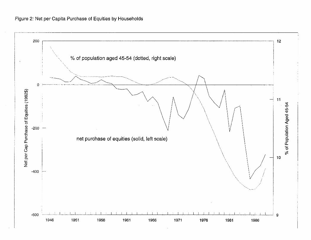
Figure 2: Net per Capita Purchase of Equities by Households

C”030)

0)43)

C.uJ4—

043)(I)

20..cL

C-)4-

43)0.

4-

43)z

200

0

-200

-400

-600

12

11

10

9

L9U~)

V43)

C0

0.00~

0

1946 1951 1956 1961 1966 1971 1976 1981 1986

Table 3: Aggregate Household Wealth

Age Group Gross Assets Net Wealth25-34 0.98

1.69-2.412.80

35-44 3.532.14

4.191.46

45-54 21.825.52

11.942.70

55-64 18.802.36

16.62.L28

65+ 8.765.08

6.403.28

adj. B2 0.49 0.47Note: t-ratios using Newey-West robust standard errors in italics.

Table 4: Age Distribution and Total Returns of Financial Assets (1926-88)

Equities BondsAge Group Common Small Co. Long Corp. Long Gov. Inter. Gov. T Bifis z~T Bills

constant 41.03 -7.45 80.60 67.44 84.23 85.65 -0.1525-34 -3.24 -1.53 -0.48 -0.31 -0.97 -1.37 -0.93

1.29 0.35 0.44 0.27 1.30 3.64 2.0335-44 6.52 3.03 1.50 1.55 1.06 0.75 0.45

1.93 0.52 1.01 1.02 1.05 1.49 0.6745-54 -17.82 -11.57 -5.98 -5.29 -6.38 -6.39 -4.29

1.70 0.64 1.31 1.12 2.06 4.08 3.5755-64 24.78 26.62 -3.03 -3.10 -0.68 0.53 -1.16

1.47 0.91 0.41 0.41 0.14 0.21 0.5865+ -9.83 -10.88 0.15 0.39 -0.63 -0.98 1.03

1.40 0.90 0.05 0.12 0.30 0.93 0.34DW 2.16 1,81 1.81 2.00 1.79 1.36 1.37

adj. B2 0.00 -0.07 0.15 0.11 0.21 0.49 0.26

Note: t-ratios using Newey-West robust standard errors in italics,

1935 1945 1955 1965 1975 1985

Figure 3: Real Annual Total Returns - Common Stock

Observed Returns

% Aged 45-54

uv

50-

40-

30-

20-

0-

-10-

-20-

-30-

.4 fl

0~’

cjqCD

-10

-11

-12

-13

-141111111--I.’-’

1925

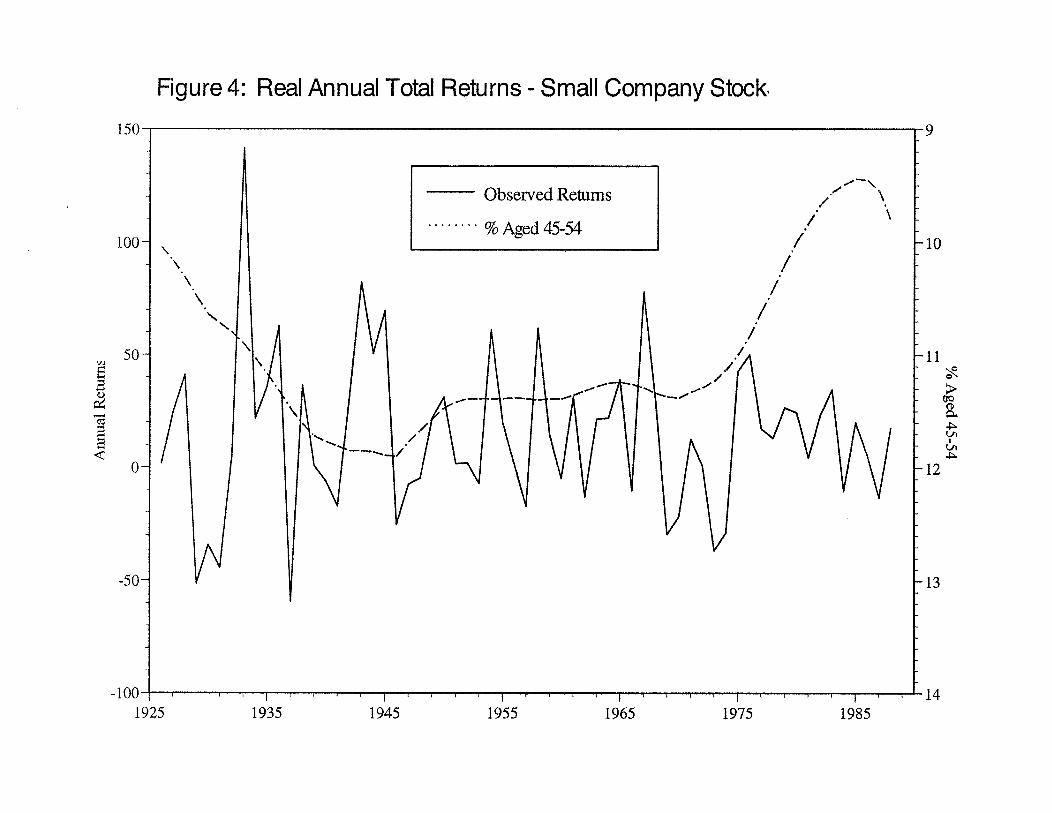
Figure 4: Real Annual Total Returns - Small Company Stock.-o

100- ___________________________ -10

~ 50- -11

III.)

a

0- ~12

-50- - 13

14— IVU I II—~

1925 1935

Observed Returns

\\

% Aged 45-54

N

1945 1955 1965 1975 1985

Figure 5: Real Annual Total Returns - Long Corporate Bonds

-20

1925 1935I I I j I I I I

40

30

\

20-

\

:7

Observed Returns% Aged 45-54

10-

0-

-10-

0~’

tjqCD

-10

-11

-12

-13

1975 198514

1945 1955 1965

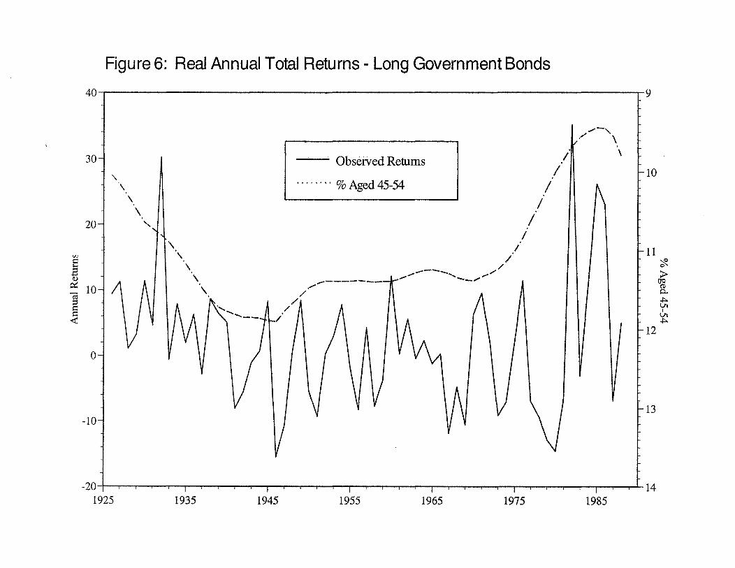
Figure 6: Real Annual Total Returns - Long Government Bonds40- -9

30

-10

20-

-11~I)CD

— lu-

-12

0-

-13-10-

—20— I I I I I I I I I I I I I i —141925 1935 1945 1955

\

\

Observed Returns

% Aged 45-54 //

/I

//

1965 1975 1985

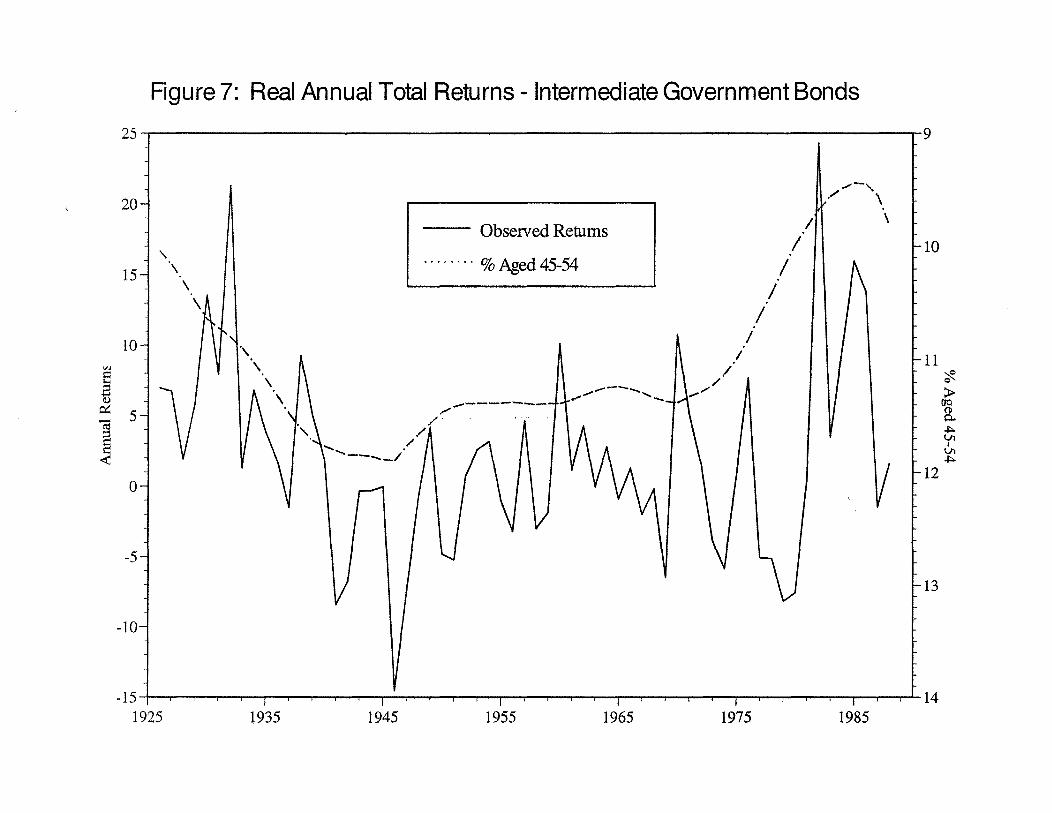
Figure 7: Real Annual Total Returns - Intermediate Government Bonds25-

20-

-10

15~

10-

-11~I)CD

— -J

L/~

-120-

-5-

-13

-10-

-15- -~ _________________________

1925

\\\

Observed Returns

% Aged 45-54 //

//

.-.-

I I I I I I I —141975 19851935 1945

I I I - I I I I I

1955 1965

Figure 8: Real Annual Total Returns - T Bills15

10-

5-

0-

-5-

-10-

-15-

-20- I I I I I1925 1935

I I I I I I I I I I I I I I I I I I

1945 1955 1965 1975

Observed Returns

NN

% Aged 45-54

//

I

.7/

//

:7

-10

-11

-12

-13

14

‘-p0~~’

1985

Figure 9: Real Annual Total Returns - T Bills (5yr centered MA)3

1

Observed Returns

% Aged 45-54

C,)

6)

0—l

CD

‘-pc~-.0

1~

-3

0.2

1925 1935 1945 1955 1965 1975 1985

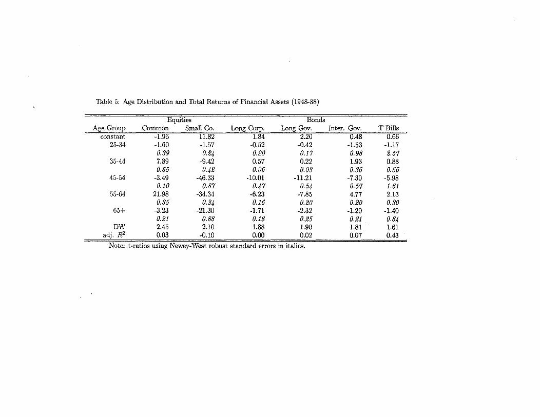
Table 5: Age Distribution and Total Returns of Financial Assets (1948-88)

Equities BondsAge Group Common Small Co. Long Corp. Long Gov. Inter. Gov. T Bills

constant -1.96 11.82 1.84 2.20 0.48 0.6625-34 -1.60 -1.57 -0.52 -0.42 -1.53 -1.17

0.39 0.24 0.20 0.17 0.98 2.5735-44 7.89 -9.42 0.57 0.22 1.93 0.88

0.55 0.42 0.06 0.03 0.36 0.5645-54 -3.49 -46.33 -10.01 -11.21 -7.30 -5.98

0.10 0.87 0.47 0.54 0.57 1.6155-64 21.98 -34.34 -6.23 -7.85 4.77 2.13

0.35 0.34 0.16 0.20 0.20 0.3065+ -3.23 -21.30 -1.71 -2.32 -1.20 -1.40

0.21 0.88 0.18 0.25 0.21 0.84DW 2.45 2.10 1.88 1.90 1.81 1.61

adj. B2 0.03 -0.10 0.00 0.02 0.07 0.43

Note: t-ratios using Newey-West robust standard errors in italics.

References

Ando, A., and Kennickell, A. B. “How Much (or Little) Life Cycle Is There

in Micro Data? The Case of the United States and Japan.” In Macroe-conomics and Finance: Essays in Honor of Franco Modigliani, edited byR. Dornbusch, S. Fischer and J. Bossons. Cambridge: MIT Press, 1987.

Auerbach, A., and Kotlikoff, L. J. Dynamic Fiscal Policy. Cambridge: Cam-bridge University Press, 1987.

Avery, R. B., and Elliehausen, G. E. “Financial Characteristics of High-income Families.” Federal Reserve Bulletin 72(1986): 163-177.

Avery, R. B.; Elliehausen, G. E.; and Canner, Glenn B. “Survey of ConsumerFinances, 1983.” Federal Reserve Bulletin 70(1984a): 679-692.

“Survey of Consumer Finances, 1983: A Second Report.” FederalReserve Bulletin 70(1984b): 857-868.

Board of Governors of the Federal Reserve System. Balance Sheet for theU.S. Economy 1949-90, 1991.

Bosworth, B.; Burtless, G.; and Sabelhaus, J. “The Decline in Savings: Ev-idence from Household Surveys.” Brookings Paper on Economic Activity1(1991): 183-256.

Bakshi, G. and Chen, Z. “Baby Boom, Population Aging and Capital Mar-kets.” Journal of Business 67(1994): 165-202.

Fair, R. C., and Dominguez, K. M. “Effects of the Changing U.S. Age Dis-tribution on Macroeconomic Equations.” American Economic Review81(1991): 1276-1294.

Hamilton, J. D. Time Series Analysis. Princeton: Princeton UniversityPress, 1994.

Lucas, R. E. “Asset Prices in an Exchange Economy.” Econometrica46(1978) 1429-1445.

Mankiw, N. G., and Weil, D. N. “The Baby Boom, the Baby Bust andthe Housing Market.” Regional Science and Urban Economics 19(1989):235-258.

Shorrocks, A. F. “TheAge-wealth Relationship: A Cross-section and CohortAnalysis.” Review of Economics and Statistics 57(1975): 155-163.

Weil, D. N. - “The Saving of the Elderly in Micro and Macro Data.”Manuscript. Cambridge: NBER, 1992.