agent-based model calibration using machine learning
TRANSCRIPT

HAL Id: hal-01499344https://hal.archives-ouvertes.fr/hal-01499344
Preprint submitted on 3 Apr 2017
HAL is a multi-disciplinary open accessarchive for the deposit and dissemination of sci-entific research documents, whether they are pub-lished or not. The documents may come fromteaching and research institutions in France orabroad, or from public or private research centers.
L’archive ouverte pluridisciplinaire HAL, estdestinée au dépôt et à la diffusion de documentsscientifiques de niveau recherche, publiés ou non,émanant des établissements d’enseignement et derecherche français ou étrangers, des laboratoirespublics ou privés.
Agent-Based Model Calibration using Machine LearningSurrogates
Francesco Lamperti, Andrea Roventini, Amir Sani
To cite this version:Francesco Lamperti, Andrea Roventini, Amir Sani. Agent-Based Model Calibration using MachineLearning Surrogates. 2017. �hal-01499344�

Agent-Based Model Calibration using MachineLearning Surrogates
Francesco Lamperti∗, Andrea Roventini† and Amir Sani‡
March 30, 2017
Abstract
Taking agent-based models (ABM) closer to the data is an open challenge. This paperexplicitly tackles parameter space exploration and calibration of ABMs combining supervisedmachine-learning and intelligent sampling to build a surrogate meta-model. The proposedapproach provides a fast and accurate approximation of model behaviour, dramaticallyreducing computation time. In that, our machine-learning surrogate facilitates large scaleexplorations of the parameter-space, while providing a powerful filter to gain insights into thecomplex functioning of agent-based models. The algorithm introduced in this paper mergesmodel simulation and output analysis into a surrogate meta-model, which substantiallyease ABM calibration. We successfully apply our approach to the Brock and Hommes(1998) asset pricing model and to the “Island” endogenous growth model (Fagiolo and Dosi,2003). Performance is evaluated against a relatively large out-of-sample set of parametercombinations, while employing different user-defined statistical tests for output analysis.The results demonstrate the capacity of machine learning surrogates to facilitate fast andprecise exploration of agent-based models’ behaviour over their often rugged parameterspaces.
Keywords: agent based model; calibration; machine learning; surrogate; meta-model.JEL codes: C15, C52, C63.
∗Corresponding author. Institute of Economics, Scuola Superiore Sant’Anna, Piazza Martiri della Liberta 33,56127 Pisa (Italy). Email: [email protected].†Institute of Economics, Scuola Superiore Sant’Anna (Pisa) and OFCE-Sciences Po (Nice). Email:
[email protected].‡Universite Paris 1 Patheon-Sorbonne and CNRS. Email: [email protected].
1

1 Introduction
This paper proposes a novel approach to model calibration and parameter space exploration inagent-based models (ABM), combining supervised machine learning and intelligent sampling inthe design of a novel surrogate meta-model.
Agent-based models deal with the study of socio-ecological systems that can be properly con-ceptualized through a set of micro and macro relationships. One problem with this frameworkis that the relevant statistical properties for variables of interest are a priori unknown, even tothe modeller Such properties emerge indeed from the repeated interactions among ecologies ofheterogeneous, boundedly-rational and adaptive agents.1 As a result, the dynamic propertiesof the system cannot be studied analytically, the identification of causal mechanisms is notalways possible and interactions give rise to the emergence of relationships that cannot simplybe deduced by aggregating those of micro variables (Anderson et al., 1972, Tesfatsion and Judd,2006, Grazzini, 2012, Gallegati and Kirman, 2012). This raises the issue of finding appropriatetools to investigate the emergent behavior of the model with respect to different parametersettings, random seeds, and initial conditions (see also Lee et al., 2015). Once this search issuccessful, one can safely move to calibration, validation and, finally, employ the model forpolicy exercises (more on that in Fagiolo and Roventini, 2017). Unfortunately, this procedureis hardly implementable in practice, notably due to large computation times.
Indeed, many ABMs simulate the evolution of complex systems with a large number ofparameters for a relatively many time steps. In a calibration setting, this rich expressiveness re-sults in a “curse of dimensionality” that lends to an exponential number of critical points alongthe parameter space, with multiple local maxima, minima and saddle points, which negativelyimpact the performance of gradient-based search procedures. Indeed, even for small models, ex-ploring the behaviour of the model through all possible parameter combinations (a full factorialexploration) is practically impossible, even employing multi-objective optimization proceduressuch as multimodel optimization or niching (for a review, see e.g. Li et al., 2013; Wong, 2015).2
However, if a model is to be used by policy makers or regulators, it must provide timely insightsinto the problem. As a result, gaining an intuition from models with rich expressiveness, butcomputationally expensive evaluations, is of limited practical interest.
Traditionally, three computationally expensive steps are involved in ABM calibration; run-ning the model, measuring calibration quality and locating parameters of interest. As remarkedin Grazzini et al. (2017), such steps account for more than half of the time required to estimateABMs, even for extremely simple models. Recently, Kriging (also known as Gaussian processes)has been employed to build surrogate meta-models of ABMs (Salle and Yildizoglu, 2014; Dosi
1In the last two decades a variety of ABM have been applied to study many different issues across a broadspectrum of disciplines beyond economics and including ecology (Grimm and Railsback, 2013), health care (Effkenet al., 2012), sociology (Macy and Willer, 2002), geography (Brown et al., 2005), bio-terrorism (Carley et al.,2006), medical research (An and Wilensky, 2009), military tactics (Ilachinski, 1997) and many others. See alsoSquazzoni (2010) for a discussion on the impact of ABM in social sciences, and Fagiolo and Roventini (2012,2017) for an assessment of macroeconomic policies in agent-based models.
2For example, consider a model with 5 parameters and assume that a single evaluation of the ABM requires5 seconds on a single compute core (CPU). If one discretizes the parameter space by splitting each dimensioninto 10 intervals, 105 evaluations would require approximately 6 CPU days to explore. With a finer partition ofof say 15 intervals, 1015 evaluations would roughly require 1.5 months, and 20 intervals would require 6 months.Adding a sixth parameter would require more than 10 years.
2

et al., 2016, 2017c,b; Bargigli et al., 2016) to facilitate parameter space exploration and sensi-tivity analyses. However, Kriging cannot be reasonably applied to large scale models with morethan 20 parameters even in the linear time extensions proposed in Wilson et al. (2015) andHerlands et al. (2015). Moreover, the smooth surfaces produced by Kriging meta-models donot provide an accurate approximation of the rugged parameter spaces characteristic of mostABMs.
In this paper, we explicitly tackle the problem of efficiently exploring the complex parameterspace of agent-based models by employing an efficient, adaptive, gradient-free search over theparameter space. The proposed approach exploits a semi-supervised notion of the parameterspace to build a fast, efficient, machine-learning surrogate that provides a mapping between thestatistic measured on the output of a specific parameterization combined and a user-definedmeasure of fit for the ABM. This procedure results in a dramatic reduction in computationtime, while providing an accurate surrogate of the original ABM that can be employed toprovide a detailed exploration of its possibly wild parameter space. Moreover, we move towardscalibration by identifying parameter combinations that allow the ABM to match user-desiredproperties.3
Surrogate meta-models are traditionally employed to approximate or emulate computation-ally costly experiments or simulation models of complex physical phenomena (see Booker et al.,1999). In particular, surrogates provide a proxy that can be exploited for fast parameter-spaceexploration and model calibration. Given their speed advantage, surrogates are regularly ex-ploited to locate promising calibration values and gain rapid intuition over a model. Notethat the objective is not to return a single optimal parameter, but all parametrizations thatpositively identify the ABM with user-desired behaviour. Accordingly, if the surrogate approx-imation error is small, it can be interpreted as an efficient and reasonably good replacement forthe original ABM during parameter space exploration and calibration.
Our approach to learning a surrogate occurs over multiple rounds. First, a large “pool” ofunlabelled parametrizations are drawn using a standard sampling routine, such as quasi-randomSobol sampling. Next, a very small subset of the pool is randomly drawn without replacement forevaluation in the ABM, making sure to have at least one example of the user-desired behaviour.These points are “labelled” according to the statistic measured on the output generated by theABM and act as a “seed” set of samples to initialize the surrogate model learned in the firstround. This first surrogate is then exploited to predict the label for unlabelled points remainingin the pool. Another very small subset of points are drawn from the pool for evaluation inthe agent-based model. Then, over multiple rounds, this process is repeated until a specifiedbudget of evaluations is achieved. In each round, the surrogate directs which unlabelled pointsare drawn from the pool to maximize the performance of the surrogate learned in the nextround. This semi-supervised “active” learning procedure incrementally improves the surrogatemodel, while maximizing the information gained over the ABM parameter space.4
3The interested reader might want to look at van der Hoog (2016) for a broad discussion on possible applica-tions of machine learning algorithms to agent based modelling.
4In the Machine Learning jargon supervised learning refers to the task of inferring a function from labeledtraining data, that is, data that are assigned either a numerical value or a symbol. Semi-supervised learningindicates a setting when there is a small amount of labelled data relatively to unlabelled ones. The term activerefers instead refers an algorithm that actively selects which data point to evaluate and, therefore, to label.
3
The performance of such a procedure crucially depends on the particular surrogate modelused in each of the rounds. Here, we automatically tune extremely boosted gradient trees (XG-Boost, see Chen and Guestrin, 2016) as our machine-learning surrogate, through automatedhyperparameter optimization (Claesen et al., 2014, see), to robustly manage non-linear pa-rameter surfaces and so-called “knife-edge” properties characteristic of ABMs. One particularadvantage of this surrogate learning algorithm over Kriging is that it does not require the selec-tion of a kernel or to set a prior in advance of the previously mentioned sampling procedure. Italso avoids the problem of choosing a summary statistic and acceptance thresholds that comeswith likelihood-free approximate Bayesian methods Grazzini et al. (2017).
As illustrative examples, we apply our procedure to two well known ABMs: the asset pricingmodel proposed in Brock and Hommes (1998) and the endogenous growth model developed inFagiolo and Dosi (2003). Despite their relative simplicity, the two models might exhibit multipleequilibria, allow different behavioural attitudes and account for a wide range of dynamics,which crucially depends on their parameters. We find that our machine-learning surrogate isable to efficiently filter out combinations of parameters conveying the output of interest, assessthe relative importance of models’ parameters and provide an accurate approximation of theunderlying ABM in a negligible amount of time. The advantages in terms of computation cost,hands-free parameter selection and ability to deal with non-linear characteristics of the ABMparameter space of our approach paves the way towards an efficient and user-friendly procedureto parameter space exploration and calibration of agent-based models.
The remaining portions of this paper are organized as follows. Section 2 reviews literatureon ABM calibration validation, making the case for surrogate modelling. Section 3 presents oursurrogate modelling methodology. Sections 4 and 5 report the results of its application to theasset pricing model proposed in Brock and Hommes (1998) and the growth model developed inFagiolo and Dosi (2003) respectively. Finally, Section 6 concludes.
2 Calibration and validation of agent-based models: the casefor surrogate modelling
As stated in Fagiolo et al. (2007) and Fagiolo and Roventini (2012, 2017), the extreme flexibilityof ABMs concerning e.g. various forms of individual behaviour, interaction patterns and institu-tional arrangements has allowed researchers to explore the positive and normative consequencesof departing from the often over-simplifying assumptions characterizing most mainstream ana-lytical models. Recent years have witnessed a trend in macro and financial modeling towardsmore detailed and richer models, targeting a higher number of stylized facts, and claiming astrong empirical content.5
A common theme informing both theoretical analysis and methodological research concernsthe relationships between agent-based models and real-world data. Recently, many studies haveaddressed the problem of estimating and calibrating ABMs. As stated by Chen et al. (2012),
5See e.g. Dosi et al. (2010, 2013, 2015); Caiani et al. (2016); Assenza et al. (2015) and Dawid et al. (2014a)on business cycle dynamics, Lamperti et al. (2017) on growth, green transitions and climate change, Dawid et al.(2014b) on regional convergence and Leal et al. (2014) on financial markets. The surveys in Fagiolo and Roventini(2012, 2017) provides a more exhaustive list.
4

ABMs need to move from stage I, i.e. the capability to grow stylized facts in a qualitative sense,to stage II, where appropriate parameter values are selected according to sound econometrictechniques. In those cases where the model is sufficiently simple and well behaved, one canderive a closed form solution for the distributional properties of a specific output of the model,and then estimating the parameters governing such distributions (see e.g. Alfarano et al., 2005,2006; Boswijk et al., 2007). However, when models’ complexity prevents to obtain closed formsolutions, more sophisticated techniques are required. Amilon (2008) estimates a model offinancial markets with 15 parameters (but only 2 or 3 agents) by efficient method of momentsand reports an high sensitivity of the model to the assumptions on the noise term and stochasticcomponents. Gilli and Winker (2003) and Winker et al. (2007) introduce an algorithm and aset of statistics leading to the construction of an objective function, which is used to estimateexchange-rate models by indirect inference, pushing them closer to the properties of real data.Franke (2009) refines on this framework and uses the method of simulated moments to estimate6 parameters of an asset pricing model, while Franke and Westerhoff (2012) propose a modelcontest for structural stochastic volatility models characterized by few parameters.6 Finally,Recchioni et al. (2015) use a simple gradient-based calibration procedure and then test theperformance of the model they obtained through out of sample forecasting.
A parallel stream of research is recently focusing on the development of tools to investigatethe extent to which agent-based models’ outputs is able to approximate reality (see Marks, 2013;Lamperti, 2017, 2016; Barde, 2016b,a; Guerini and Moneta, 2016). Some of these contributionsalso offer new measures that can be used to build objective functions in the place of longitudinalmoments within an estimation setting (e.g. the GSL-div introduced in Lamperti, 2017). How-ever, a common limitation of both these calibration/estimation and validation exercises lies intheir computational time, which is usually extremely high. As well discussed in Grazzini et al.(2017), the most consuming step of all these procedures consists in simulating the model. Forinstance, in order to train his algorithm, Barde (2016b) needs Monte Carlo (MC) runs eachhaving length of about 219 periods, and many macroeconomic ABMs might take weeks justto perform a single MC exercise of this kind. This explains why the vast majority of previouscontributions employ extremely simple ABMs (few parameters, few agents, no stochastic draws)to illustrate their approach, and large macro ABMs are usually poorly validated and calibrated.Hence, using standard statistical techniques, the number of parameters must be minimized toachieve feasible estimation.
From a theoretical perspective, the curse of dimensionality implies that the convergence ofany estimator to the true value of a smooth function defined on a high dimensional parameterspace is very slow (Weeks, 1995; De Marchi, 2005). Several methods have been introduced in thedesign of experiments literature to circumvent this problem, but the assumptions of smoothness,linearity and normality do not generally hold for ABMs (see the extensive discussion in Lee et al.,2015).
Unfortunately, recent developments in agent-based macro-economics have led to the devel-opment of more and more complex models, which require large sets of parameters to adequatelycapture the complexity of micro-founded, multi-sector and possibly multi-country phenomena
6See also Grazzini and Richiardi (2015) and Fabretti (2012) for other applications of the same approach
5

(see Fagiolo and Roventini, 2017, for a recent survey). In such a setting, neither direct estima-tions nor global sensitivity analysis (often advocated as a natural approach to ABM exploration,cf. Moss, 2008; Thiele et al., 2014; ten Broeke et al., 2016) seem computationally feasible.
New alternative methods must deal with two issues: reduction in computation time and thedesign of appropriate criteria for calibration and validation procedures. Our approach showsthat such issues can be related in a meaningful way by developing a computational procedurethat efficiently trains a surrogate model in order to optimize specific calibration criteria orreproducing statistical relationships between model-generated variables. Our procedure hassome similarities to the one of Dawid et al. (2014b), where penalized splines methods areemployed to shortcut parameter exploration and unravel the dynamic effects of policies onthe economic variables of interest. However, our method especially focuses on computationalefficiency and therefore builds on two pillars: surrogate modelling and intelligent sampling.
With respect to surrogate modelling, we extend recent contributions in the economic liter-ature that use kriging to build a surrogate meta-model for ABMs (Salle and Yildizoglu, 2014;Dosi et al., 2017c; Bargigli et al., 2016). One of the primary challenges with kriging-basedmeta-models is that they cannot efficiently model more than a dozen parameters. This con-straint forces modellers to arbitrarily fix a subset of parameters whenever the parameter space islarge. Moreover, kriging relies on Gaussian processes (Rasmussen and Williams, 2006; Conti andO’Hagan, 2010), which face serious difficulties when the underlying smoothness assumptions areviolated. Modelling the rugged parameter space of ABMs is particularly challenging. In orderto overcome these constraints, our meta-modelling approach leverages non-parametric boostedtrees from the machine learning literature that do not depend on smoothness assumptions (seeFreund et al., 1996; Breiman et al., 1984).
Even the most advanced surrogate modelling algorithm only performs as well as the qualityof labelled samples. With respect to ABMs, a labelled sample is a parameter combination andthe output of the ABM given this parametrization. Batch sampling, the process of sampling abudget of samples all at once, such as in random sampling, quasi-random sampling (e.g. Sobolsampling), extensions that extend the Sobol sequence to reduce error rates (see Saltelli et al.,2010) and more sophisticated procedures such as Latin-Hypercube sampling are all limitedby their one-off nature to sampling. Further, ABM parameters of interest are often rare andrepresent a small percent of possible parametrizations. Given this imbalanced nature of thesample and the non-negligible computation cost of evaluating ABM parameters, it makes senseto carefully select which parametrizations to evaluate, while exploiting the cheap (almost free)cost of generating unevaluated parametrizations. The problem of sequentially selecting themost informative subset of samples over multiple sampling rounds underlies active learning (seeSettles, 2010, for a survey). In particular, given a pool of unlabelled parametrizations, and afixed evaluation budget, active learning chooses parametrizations from the pool that maximizesthe performance of the surrogate meta-model.
6

3 Surrogate modelling methodology
In all generality, one can represent an agent-based model as a mapping m : I → O from aset of input parameters I into an output set O. The set of parameters can be conceived asa multidimensional space spanned by the support of each parameter. Usually, the numberof parameters go from 1 or 2 to few dozens, as in large macro models. The output set isgenerally larger, as it corresponds to time-series realizations of a very large number of microand macro level variables. This rich set of outputs allows a qualitative validation of agent-based models based on their ability to reproduce the statistical properties of empirical data(e.g. non-stationarity of GDP, cross-correlations and relative volatilities of macroeconomic timeseries), as well as microeconomic distributional characteristics (e.g. distribution of firms’ size,of households’ income, of assets’ returns). Beyond stylized facts, the quantitative validationof an agent-based model also requires the calibration/estimation of the model on a (generallysmall) set of aggregate variables (e.g. GDP growth rates, inflation and unemployment levels,asset returns etc.).
Without loss of generality, we can represent this quantitative calibration as the determinationof input values such that the output satisfies certain calibration conditions, coming from, e.g,a statistical test or the evaluation of a likelihood or loss functions. This is in line, for example,with the method of simulated moments (Gilli and Winker, 2003; Franke and Westerhoff, 2012).We consider two settings:
• Binary outcome. In this setting the calibration criterion can be considered as a function,v : O → {0, 1}, that maps the ABM output to a binary variable that takes 1 if a certainproperty of the output (or set of properties) is found, and 0 otherwise. For example, aproperty that one might want a financial ABM to match is the presence of excess kurtosisin the distribution of returns. This setting leads to what is referred in the machine learningliterature as a classification problem.
• Real-valued outcome. In this setting the calibration criterion can be considered as afunction, v : O → R, that maps the ABM output to a real valued number providing aquantitative assessment of a certain property of the model. For example, one might wantto compute excess kurtosis of simulated data and then compare it to the one obtainedfrom real data. This setting leads to what is referred in the machine learning literatureas a regression problem.
To keep consistency with the machine learning jargon, we say that the value that functionv assigns to parameter vector x is called label of x. Obviously, one would like to find the setof input parameters x ∈ I such that their labels indicate that a chosen condition is met. Moreformally, we say that C is the set of labels indicating that the condition is satisfied. For example,in the case of binary outcome we can say that C = {1}, which indicates that the chosen propertyis observed; in the case of real valued outcome, assuming that v expresses the distance betweensome statistic of the simulated and real data, one might consider C = {x : v(x) ≤ α} orC = {minx∈Ij v(x), j = 1, 2, 3, .., J}. The latter case reflects exactly the common calibration
7

problem of minimizing some loss function over the parameter space with random restart toavoid ending up in local minima.
Definition 1. We say that a positive calibration is a parameter vector x ∈ I whose label incontained in the set C, i.e. x : v(x) ∈ C. By contrast, a negative calibration is a parametervector whose label is not contained in C.
The problem now is to find all positive calibrations. However, an intensive exploration ofthe input set I is computationally infeasible. As emphasized above, it is crucial to drasticallyreduce the computation time required to identify positive calibrations.
This paper proposes to train a surrogate model that efficiently approximates the value off(x) = v◦m(x) using a limited number of input parameters (budget) to evaluate the true ABM.Once the surrogate is trained, it provides an efficient mean of exploring the behaviour of theABM over the entire parameter space.7
The surrogate training procedure requires three decisions:
1. choosing a machine learning algorithm to act as a surrogate for the original ABM, takingcare that the assumptions made by the machine learning model do not force unrealisticassumptions on the parameter space;
2. selecting a sampling procedure to draw samples from the parameters space in order totrain the surrogate;
3. selecting a score or criterion that can be used to evaluate the performance of the surrogate.
As for the construction of the surrogate, we want to avoid smoothness assumptions and thechallenge of selecting the correct prior and kernel in kriging-based methods (see Rasmussen andWilliams, 2006; Ryabko, 2016), so we propose to use extreme gradient boosted trees (XGBoost)(Chen and Guestrin, 2016, see), which is composed of a random ensemble (see Breiman, 2001)of “boosted” (see Freund, 1990; Freund et al., 1996) classification and regression trees (CART)(Breiman et al., 1984, see). This choice endows our surrogate with the ability to learn non-linear “knife-edge” properties, which typically characterize ABM parameter spaces. Samplingshould carefully select which parametrizations of an ABM should be evaluated according tothe performance of the surrogate. Here, we leverage pool-based active learning according to apre-specified budget of evaluations8 The structure of the surrogate, active learning approachand performance criterion are detailed below.
3.1 Structure of the surrogate
Here, we employ an iterative training procedure (see Figure 1) to construct a different surrogateat each of several rounds until we approach a predefined budget of evaluations on the true ABM.At each round an additional parameter vectors is used in the iterative procedure. The budget
7Notwithstanding its precision, the surrogate remains an approximation of the original model. We suggestthe user, in any case, to identify positive calibrations and further study model’s behaviour therein and in theirclose neighbourhoods employing the original ABM.
8For a review of active learning, see e.g. Settles (2010).
8

Figure 1: Surrogate modelling algorithm.
is set in advance by the user according to a pre-determined, acceptable, computation cost oflearning the surrogate. In each round, a surrogate is trained using all available parametervectors, and their respective labels, which have been aggregated up to that round. Once thebudget of evaluations is reached, the final surrogate is ready to be used for parameter spaceexploration.
Here, we rely on XGBoost (Chen and Guestrin, 2016) as our surrogate learning algorithm.This algorithm sequentially learns an ensemble of classification and regression trees (CART,see Breiman et al., 1984). Figure 2 provides an example of CART tree. Given that the CARTtrees are represented as functions, the gradient resulting from the ensemble of CART trees canbe minimized. Weights are assigned to each of the parameter vectors and “boosted” in thedirection of the gradient that minimizes the total loss. Boosting magnifies the importance ofdifficult-to-learn samples. In each of the subsequent rounds, a new tree is learned over theboosted parameter vectors, incurring an increased penalty according to the boosted weights.Accordingly, trees are learned according to the weight from the previous round. The XGBoostalgorithm builds CART trees that are increasingly specialized to handle the particular subset ofsamples that were difficult to learn up until the current round. A common way to characterizethis learning procedure is to consider it as an ensemble of “weak” approximations, that togetherconstruct a strong approximation (see Freund, 1990; Freund et al., 1996; Chen and Guestrin,2016, for more details see).
3.2 Surrogate performance evaluation
A trained surrogate can be used to efficiently explore the behaviour of the ABM over the entireparameter space. Relevant parameter combinations can then be selected for evaluation usingthe original ABM. Given the desire to avoid evaluating the computationally expensive trueABM, while also identifying positive calibrations, it is critical to maximize the performanceof the surrogate to predict these calibrations. We recall that positive calibrations are pointsin the parameter space that fulfil the specific conditions, specified by an ABM modeller/user.Such conditions might include any test that compares simulated output with real data (e.g.distance between real and simulated moments, a non-parametric test on distribution equality,mean squared prediction errors, etc.) and/or any specific feature the model might generate (e.g.
9

Figure 2: An example classification and regression tree (CART) used for regression. Featuresare labelled f0, . . . , f4 and nodes specify cut-off thresholds that designate the path a newparameter vector takes from the top (root) node to the final (leaf) node, which denotes thepredicted calibration value. In the process of “boosting” CART trees to produce an ensemble,each subsequent tree increasingly focuses on the higher weighted samples. This generally resultsin smaller “specialized” trees that stick on samples that were most difficult to classify.
fat tails in a specific distribution, growth rates of any variable above or below a given threshold,correlation patterns among a set of variables, etc.). In the two exercises presented in this paper(cf. Sections 4 and 5 below), both types of conditions are evaluated.
An effective surrogate should maximize the “True Positive Rate” (TPR). Given a set ofparameter combinations, the TPR measures the number of positive calibrations predicted bya learned surrogate model against the actual number of positive calibrations possible in theparameter space. Automated hyper-parameter optimization procedures maximize the perfor-mance of the machine learning surrogate according to a learning score or metric.9 Though our
9Several procedures exist for tuning machine learning hyper-parameters, see e.g. Feurer et al. (2015).
10
aim is to maximize the TPR of our surrogate, the scores used to train the surrogate depend onthe particular form of the output condition. According to the two settings introduced above wedistinguish between:
• Binary outcome. In this case the output of the calibration condition is discrete, suchas Accept/Reject, and a measure of classification ability is needed. Specifically, we aim atmaximizing the F1-score.10 The F1-score is an harmonic mean between p, which indicatesthe ratio between true positives and total positives and r, which represents the ratio oftrue positives to predicted ones:
F1 = 2 p · rp+ r
, (1)
The F1-score takes a value between 0 and 1. In terms of Type I and Type II errors, itequates to:
F1 = 2 · true positives2 · true positives + false positives + false negatives . (2)
• Real-valued outcome. In this case, our aim is to minimize the mean-squared error(MSE),
MSE =∑Ni=1(yi − yi)2
N, (3)
where the surrogate predicts yi over N evaluation points with a true labelling y. We noticethat this approach is in line, for instance, with Recchioni et al. (2015).
3.3 Parameter importance
The XGBoost algorithm employed in our surrogate modelling procedure allow us also to performparameter sensitivity analysis at no costs. In particular, the machine learning algorithm providesan intuitive procedure of assessing the explained variance of the surrogate according to therelative number of times a parameter was “split-on” in the ensemble (for details see e.g. Archerand Kimes, 2008; Louppe et al., 2013; Breiman, 2001). As each tree is constructed according toan optimized splitting of the possible values for a specific parameter vector, and it is increasinglyfocusing on difficult-to-predict samples, splits dictate the relative importance of parameters indiscriminating the output conditions of the ABM. Accordingly, the relative number of splits overa specific parameter provides a quantitative assessment of the sensitivity of the surrogate to theparameter and importance of that parameter to the user-specified conditions. As a consequence,this allows to rank model’s parameters on the basis of their importance in producing a behaviourof the model that satisfy whatever condition the user specifies. As this procedure is non-parametric, the resulting values should be interpreted as a rank-based statistic. The particularvalues associated to the number of splits only characterize the specific instantiation of theensemble. Specifically, a different number of trees would result in changes to the split countfor each feature. The resulting counts provide insight into the relative performance for each
10Note that there is “no free lunch” with regard to performance measures, so their choice depends on theproblem setting (see e.g. Wolpert, 2002) For a detailed description of the F1-Score, see e.g. Van Rijsbergen(1979).
11
parameter. As the number of trees approaches infinity, the number of splits will converge tothe true ratio per feature by the law of large numbers.
3.4 Training procedure
The primary constraint we face is the limited number of parameter combinations that can beused for model evaluation (budget) without incurring in excessive computational costs. Toaddress this issue, we propose a budgeted online active semi-supervised learning approach thatiteratively builds a training set of parameter vectors on which the agent-based model is actuallyevaluated in order to provide labelled data points for the training of the surrogate. The aimof actively sampling the parameter space is to reduce the discrepancy between the regions thatcontain a manifold of interest and the function approximation produced by the surrogate model.This semi-supervised learning approach (see e.g. Zhu, 2005; Goldberg et al., 2011) minimizesthe number of required evaluations, while improving the performance of the surrogate. Giventhat evaluated parametrizations are aggregated over several rounds and the stationary natureof the parameter space labels, we can use the log convergence results proved in Ross et al.(2011) to provide a guideline on the number of parametrizations to evaluate in each round. Inparticular, we set the initial starting round to include at least one positive calibration and eachof the subsequent rounds to log budget.
Our active learning approach relies on the assumption that positive calibrations representa very small percentage of points in the parameter space. Leveraging on such an imbalance,our approach iteratively selects a random subset of positive predicted calibrations over a finitenumber of rounds. In order to maximize computing speed, the algorithm is initialized with afixed subset of evaluated parameter combinations that are drawn according to a quasi-randomSobol sampling over the parameter space (Morokoff and Caflisch, 1994).11 Further, the numberof samples are drawn according to the ones required for “total variation” analysis presented inSaltelli et al. (2010). These initial “training” points are then evaluated through the ABM, theirlabels recorded and finally used to initialize the first surrogate model. Once the surrogate istrained, new parameter combinations are sampled over the entire parameter space and labelledusing the surrogate. A random subset of points xi are then selected from the predicted positivecalibrations of the surrogate and evaluated for their true labels yi using the ABM. Given thelog convergence rates presented in
These new points are then added to the training set to train a new surrogate in the nextround. This “self-training” procedure exploits the imbalance in the data to incrementally in-crease true positives, while reducing false positives. Note that this simple self-training proceduremay result in no new predicted positives. In this case, the algorithm selects new points accord-ing to their predicted binary label entropy, where the latter is defined as the entropy betweenthe predicted positive and negative calibration label probabilities. This incremental procedurecontinues until the targeted training budget is achieved. The algorithm pseudo-code is presentedin Figure 3.
11Note that in high dimensional spaces, standard design of experiments are computationally costly and showlittle or no advantage over random sampling (Bergstra and Bengio, 2012; Lee et al., 2015).
12

Set:
• Agent Based Model ABM ∈ RJ
• Sampling distribution ν ∈ RJ
• Calibration function C(·)
• Learning algorithm A, with parameters Θ
• Evaluation budget B
• Initial training set size N � B
• XT raining ∈ RN×J
• Calibration labels Y T raining ∈ NN binary outcome case (at least 1 positivecalibration)
• Calibration labels Y T raining ∈ RN real-valued outcome case (at least 1 posi-tive calibration)
• Hyper-parameter optimization algorithm (HPO)
Initialize:
• Per-round sampling size S � B
• Per-round out-of-sample size K � B
While |Y | < B, repeat
1. Θ = HPO(A(Θ, XT raining, Y T raining))
2. Draw out-of-sample points XOOS ∈ RK×J ∼ ν
3. Select Xsample ∈ RS×J from XOOS
4. Evaluate XT raining = XT raining ∪Xsample
5. Evaluate Y sample = {C(ABM(Xsamplei ))}i=1...S
6. Evaluate Y T raining = Y T raining ∪ Y sample
end while
Figure 3: Pseudo-code of our training algorithm. Note: Y indicates labels; X indicates param-eter vectors. HPO: hyper parameter optimization; OOS: out of sample
13

4 Surrogate modelling examples: The Brock and Hommes model
In their seminal contribution, Brock and Hommes (1998) develop an asset pricing model (re-ferred here as B&H), where an heterogeneous population of agents trade a generic assets ac-cording to different strategies (fundamentalist, chartists, etc.). In what follow, we first brieflyintroduce the model (cf. Section 4.1). We then report the empirical setting (see Section 4.2) andthe results of our machine learning calibration and exploration exercise (cf. Section 4.3). Werecall that the seed of the pseudo-random number generator is fixed and kept constant acrossruns of the model over different parameter vectors.
4.1 The B&H asset pricing model
There is a population of N traders that can invest either in a risk free asset, which is perfectlyelastically supplied at a gross return R = (1+r) > 1, or in a risky one, which pays an uncertaindividend y and has a price denoted by p. Wealth dynamics is given by
Wt+1 = RWt + (pt+1 + yt+1 −Rpt)zt, (4)
where pt+1 and yt+1 are random variables and zt is the number of the shares of the risky assetbought at time t.
Traders are heterogeneous in terms of their expectations about future prices and dividendsand are assumed to be myopic mean-variance maximizers. However, as information about pastprices and dividends is publicly available in the market, agents can apply conditional expectedvalue Et, and variance Vt. The demand for share zh,t of agents with expectations of type h iscomputed solving:
maxzh,t
{Eh,t(Wt+1)− ν
2Vh,t(Wt+1)}, (5)
which in turns implieszh,t = Eh,t(pt+1 + yt+1 −Rpt)/(νσ2), (6)
where ν controls for agents’ risk aversion and σ indicates the conditional volatility, assumed tobe equal across traders and constant over time. In case of zero supply of outside shares anddifferent trader types, the market equilibrium equation can be written as:
Rpt =∑
nh,tEh,t(pt+1 + yt+1), (7)
where nh,t denotes the share that traders of type h hold at time t. In presence of homogeneoustraders, perfect information and rational expectations, one can derive the no-arbitrage marketequilibrium condition:
Rp∗t = Et(p∗t+1 + yt+1), (8)
where the expectation is conditional on all histories of prices and dividends up to time t andwhere p∗ indicates the fundamental price. In case dividends are independent and identicallydistributed over time with constant mean, equation (8) has a unique solution where the fun-damental price is constant and equal to p∗ = E(yt)/(R − 1). In what follows, we will express
14

prices as deviations from the fundamental price, i.e. xt = pt − p∗t .At the beginning of each trading period t = {1, 2, ..., T}, agents form expectations about
future prices and dividends. Agents are heterogeneous in their forecasts. More specifically,investors believe that, in a heterogeneous world, prices may deviate from the fundamental valueby some function fh(·) depending upon past deviations from the fundamental price. Accordingly,the beliefs about pt+1 and yt+1 of agents of type h evolve according to:
Eh,t(pt+1 + yt+1) = Et(p∗t+1) + fh(xt−1, ..., xt−L). (9)
Many forecasting strategies specifying different trading behaviours and attitudes have beenstudied in the economic literature, (see e.g. Banerjee, 1992; Brock and Hommes, 1997; Luxand Marchesi, 2000; Chiarella et al., 2009). Brock and Hommes (1998) adopt a simple linearrepresentation of beliefs:
fh,t = ghxt−1 + bh, (10)
where gh is the trend component and bh the bias of trader type h. If bh 6= 0, the agent hcan be either a pure trend chaser if gh > 0 (strong trend chaser if g > R), or a contrarian ifg < 0 (strong contrarian if g < R). If gh 6= 0, the agent of type h is purely biased (upward ordownward biased if bh > 0 or bh < 0). In the special case when both gh and bh are equal tozero, the agent is a “fundamentalists”, i.e. she believes that prices return to their fundamentalvalue. Agents can also be fully rational, with frational,t = xt+1. In such a case, they have perfectforesight but, they must pay a cost C.12
In our application, we use a simple model with only two types of agents, whose behavioursvary according to the choice of trend components, biases and perfect forecasting costs. Com-bining equations (7), (9) and (10), one can derive the following equilibrium condition:
Rxt = n1,tf1,t + n2,tf2,t, (11)
which allows to compute the price of the risky asset (in deviation from the fundamental) attime t.
Traders switch among different strategies according to the their evolving profitability. Morespecifically, each strategy h is associated with a fitness measure of the form:
Uh,t = (pt + yt −Rpt−1)zh,t − Ch + ωUh,t−1 (12)
where ω ∈ [0, 1] is a weight attributed to past profits. At the beginning of each period, agentsreassess the profitability of their trading strategy with respect to the others. The probabilitythat an agent choose strategy h is given by:
nh,t = exp(βUh,t)∑h exp(βUh,t)
, (13)
12In our experiments we allow for the possibility that a positive cost might be by paid also by non-rationaltraders. This mirrors the fact that some trader might want to buy additional information, which they might notbe able to use (due e.g. to computational mistakes).
15
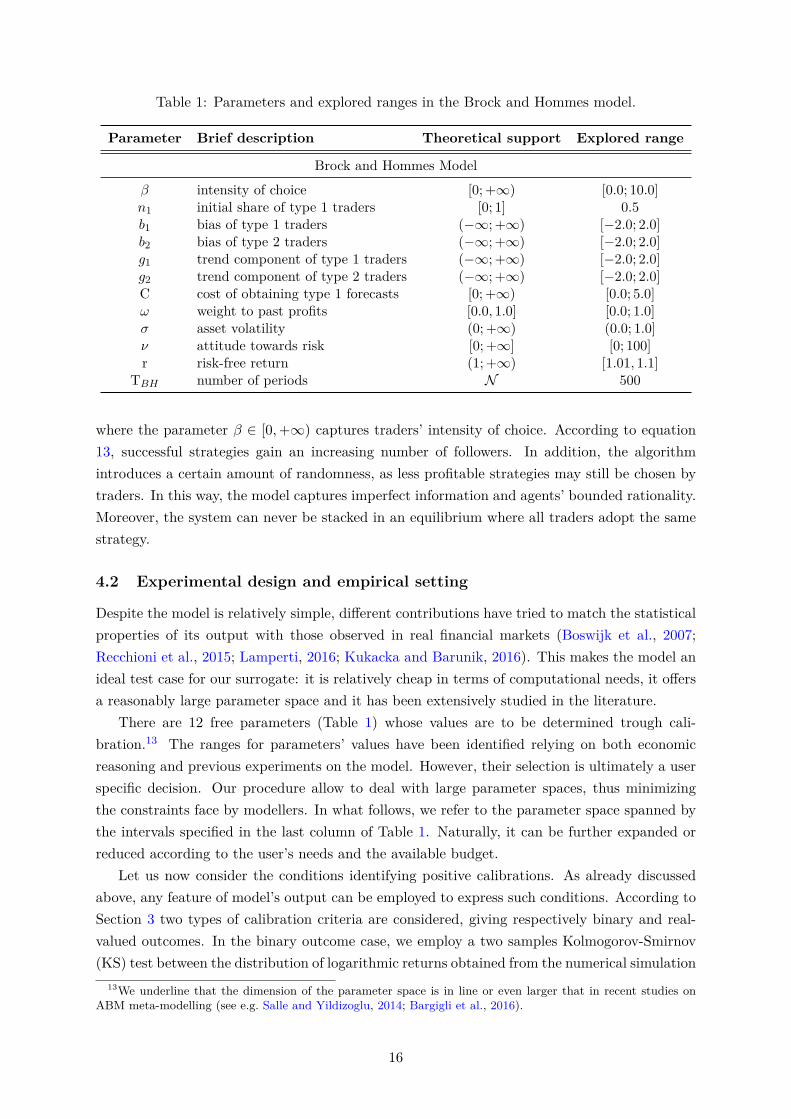
Table 1: Parameters and explored ranges in the Brock and Hommes model.
Parameter Brief description Theoretical support Explored range
Brock and Hommes Model
β intensity of choice [0; +∞) [0.0; 10.0]n1 initial share of type 1 traders [0; 1] 0.5b1 bias of type 1 traders (−∞; +∞) [−2.0; 2.0]b2 bias of type 2 traders (−∞; +∞) [−2.0; 2.0]g1 trend component of type 1 traders (−∞; +∞) [−2.0; 2.0]g2 trend component of type 2 traders (−∞; +∞) [−2.0; 2.0]C cost of obtaining type 1 forecasts [0; +∞) [0.0; 5.0]ω weight to past profits [0.0, 1.0] [0.0; 1.0]σ asset volatility (0; +∞) (0.0; 1.0]ν attitude towards risk [0; +∞] [0; 100]r risk-free return (1; +∞) [1.01, 1.1]
TBH number of periods N 500
where the parameter β ∈ [0,+∞) captures traders’ intensity of choice. According to equation13, successful strategies gain an increasing number of followers. In addition, the algorithmintroduces a certain amount of randomness, as less profitable strategies may still be chosen bytraders. In this way, the model captures imperfect information and agents’ bounded rationality.Moreover, the system can never be stacked in an equilibrium where all traders adopt the samestrategy.
4.2 Experimental design and empirical setting
Despite the model is relatively simple, different contributions have tried to match the statisticalproperties of its output with those observed in real financial markets (Boswijk et al., 2007;Recchioni et al., 2015; Lamperti, 2016; Kukacka and Barunik, 2016). This makes the model anideal test case for our surrogate: it is relatively cheap in terms of computational needs, it offersa reasonably large parameter space and it has been extensively studied in the literature.
There are 12 free parameters (Table 1) whose values are to be determined trough cali-bration.13 The ranges for parameters’ values have been identified relying on both economicreasoning and previous experiments on the model. However, their selection is ultimately a userspecific decision. Our procedure allow to deal with large parameter spaces, thus minimizingthe constraints face by modellers. In what follows, we refer to the parameter space spanned bythe intervals specified in the last column of Table 1. Naturally, it can be further expanded orreduced according to the user’s needs and the available budget.
Let us now consider the conditions identifying positive calibrations. As already discussedabove, any feature of model’s output can be employed to express such conditions. According toSection 3 two types of calibration criteria are considered, giving respectively binary and real-valued outcomes. In the binary outcome case, we employ a two samples Kolmogorov-Smirnov(KS) test between the distribution of logarithmic returns obtained from the numerical simulation
13We underline that the dimension of the parameter space is in line or even larger that in recent studies onABM meta-modelling (see e.g. Salle and Yildizoglu, 2014; Bargigli et al., 2016).
16

of the model and the one obtained from real stock market data.14 More specifically, we rely ondaily adjusted closing prices for the S&P 500 going from December 09, 2013 to December 07,2015, for a total of 502 observations, and we compute the following test statistic:15
DRW,S = supr|FRW (r)− FS(r)|, (14)
where r indicate logarithmic returns and FRW and FS are the empirical distribution functionsof the real world (RW ) and simulated (S) samples respectively. Then, in a real-valued outcomesetting, we use the p-value of the KS test, P (D > DRW,S), as an expression of model’s fitwith the data. In particular, the higher the p-value of the test, the more difficult to rejectthe null and the larger the fit with the data. We also consider an equivalent condition forthe binary outcome: predicted labels above 5% indicate positive calibrations. The choice ismade on purpose: using equivalent conditions allows to compare the binary and real-valuedoutcome in terms of precision (ability to identify true calibrations) and computational time (inthe real-valued scenario there is more information to be processed.)
We train the surrogate 100 times over 10 different budgets of 250, 500, 750, 1000, 1250, 1500,1750, 2000, 2250, 2500 labelled parameter combinations and evaluate it on 100000 unlabelledpoints. Having a large number of out-of-sample, unlabelled, possibly well-spread points isfundamental to evaluate the performance of the meta-model. We use a larger evaluation set thanany other meta-modelling contribution we are aware of (see, for instance, Salle and Yildizoglu,2014; Dosi et al., 2017c; Bargigli et al., 2016).
4.3 Results
In Figure 4, we show the parameter importance results for the Brock and Hommes (B&H)model. We find that the most relevant parameters to fit the empirical distribution of returnsobserved in the SP500 are those characterizing traders’ attitude towards the trend (g1 and g2)and, secondly, their bias (b1 and b2). This result is in line with recent findings by Recchioni et al.(2015) and Lamperti (2016) obtained using the same model. Moreover, the intensity of choiceparameter (β, cf. Section 4), which is of crucial importance in the original model developed byBrock and Hommes (1998), does not appear to be particularly relevant in determining the fitof the model with the data if compared to other behavioural parameters (at least within therange expressed by Table 1, ).16 Also traders’ risk attitude (α) and the weight associated topast profits (ω) are relatively unimportant to shape the empirical performance of the model.
Let us now consider the behaviour of the surrogate. As outlined in Section 3.2, we runa series of exercises where the surrogate is employed to explore the behaviour of the modelover the parameter space and filter out positive calibrations matching the distribution of realstock-market returns. Figure 5 collects the results and show the performance of the surrogatein the two proposed settings (binary and real-valued outcome). Within the binary outcome
14Let pt and pt−1 be the prices of an asset at two subsequent time steps. The logarithmic return from t− 1 tot is given by rt = log(pt/pt−1) ' (pt − pt−1)/pt−1.
15The data have been obtained from Yahoo Finance: https://finance.yahoo.com/quote/%5EGSPC/history.The test is passed if the null hypothesis “equality of the distributions” is not rejected at 5% confidence level.
16See also Boswijk et al. (2007) where the authors estimate the B&H model on the SP500 and, in manyexercises, find the switching parameter not to be significant.
17
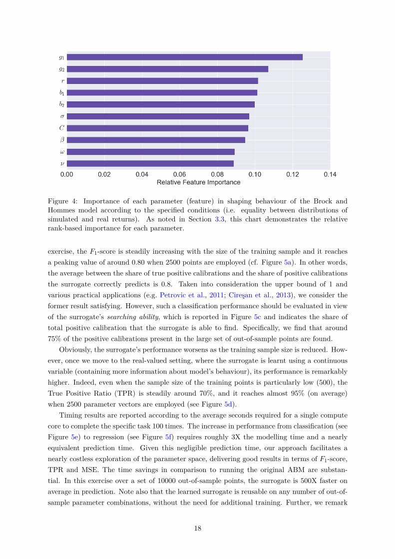
Figure 4: Importance of each parameter (feature) in shaping behaviour of the Brock andHommes model according to the specified conditions (i.e. equality between distributions ofsimulated and real returns). As noted in Section 3.3, this chart demonstrates the relativerank-based importance for each parameter.
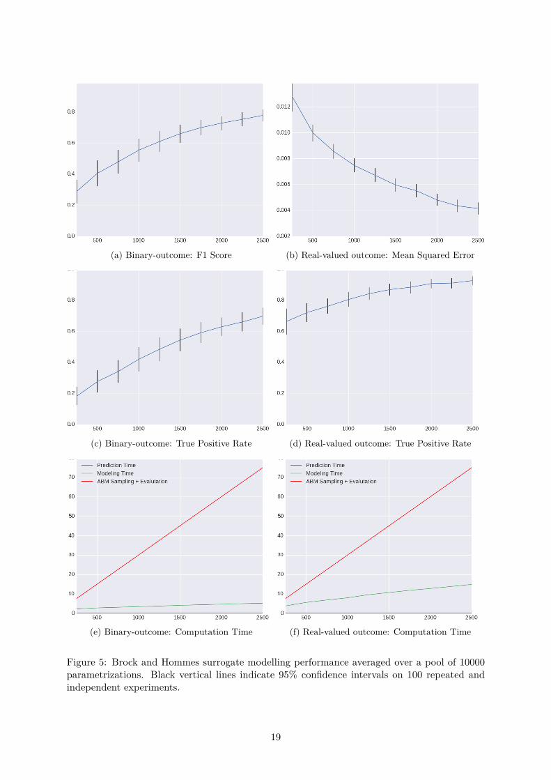
exercise, the F1-score is steadily increasing with the size of the training sample and it reachesa peaking value of around 0.80 when 2500 points are employed (cf. Figure 5a). In other words,the average between the share of true positive calibrations and the share of positive calibrationsthe surrogate correctly predicts is 0.8. Taken into consideration the upper bound of 1 andvarious practical applications (e.g. Petrovic et al., 2011; Ciresan et al., 2013), we consider theformer result satisfying. However, such a classification performance should be evaluated in viewof the surrogate’s searching ability, which is reported in Figure 5c and indicates the share oftotal positive calibration that the surrogate is able to find. Specifically, we find that around75% of the positive calibrations present in the large set of out-of-sample points are found.
Obviously, the surrogate’s performance worsens as the training sample size is reduced. How-ever, once we move to the real-valued setting, where the surrogate is learnt using a continuousvariable (containing more information about model’s behaviour), its performance is remarkablyhigher. Indeed, even when the sample size of the training points is particularly low (500), theTrue Positive Ratio (TPR) is steadily around 70%, and it reaches almost 95% (on average)when 2500 parameter vectors are employed (see Figure 5d).
Timing results are reported according to the average seconds required for a single computecore to complete the specific task 100 times. The increase in performance from classification (seeFigure 5e) to regression (see Figure 5f) requires roughly 3X the modelling time and a nearlyequivalent prediction time. Given this negligible prediction time, our approach facilitates anearly costless exploration of the parameter space, delivering good results in terms of F1-score,TPR and MSE. The time savings in comparison to running the original ABM are substan-tial. In this exercise over a set of 10000 out-of-sample points, the surrogate is 500X faster onaverage in prediction. Note also that the learned surrogate is reusable on any number of out-of-sample parameter combinations, without the need for additional training. Further, we remark
18
(a) Binary-outcome: F1 Score (b) Real-valued outcome: Mean Squared Error
(c) Binary-outcome: True Positive Rate (d) Real-valued outcome: True Positive Rate
(e) Binary-outcome: Computation Time (f) Real-valued outcome: Computation Time
Figure 5: Brock and Hommes surrogate modelling performance averaged over a pool of 10000parametrizations. Black vertical lines indicate 95% confidence intervals on 100 repeated andindependent experiments.
19
that computational gains are expected to be larger as more complex and expensive-to-simulatemodels are used. The next section goes in this direction.
5 Surrogate modelling examples: the Islands model
In the “Island” growth model (Fagiolo and Dosi, 2003), a population of heterogeneous firms lo-cally interact discovering and diffusing new technologies, which ultimately lead to the emergence(or not) of endogenous growth. After having presented the model (Section 5.1), we describethe empirical setting (see Section 5.2) and the results of the machine learning calibration andexploration exercises (cf. Section 5.3). We recall that the seed of the pseudo-random numbergenerator is fixed and kept constant across runs of the model over different parameter vectors.
5.1 The Island growth model
A fixed population of heterogeneous firms (I = 1, 2, ..., N) explore an unknown technologicalspace (“the sea”), punctuated by islands (indexed by j = 1, 2, ...) representing new technologies.The technological space is represented by a 2-dimensional, infinite, regular lattice endowed withthe Manhattan metrics d1. The probability that each node (x, y) is an island is equal top(x, y) = π. There is only one homogeneous good, which can be “mined” from any island. Eachisland is characterized by a productivity coefficient sj = s(x, y) > 0. The production of agent ion island j having coordinates (xj , yj) is equal to:
Qi,t = s(xj , yj)[mt(xj , Yj)]α−1, (15)
where α ≥ 1 and mt(xj , yj) indicates the total number of miners working on j at time t. TheGDP of the economy is simply obtained summing up the production of each island.
Each agent can choose to be a miner and produce an homogeneous final good in her currentisland, to become an explorer and search for new islands (i.e. technologies), or to be an imitatorand seal towards a known island.
In each time step, miners can decide to become explorer with probability ε > 0. In thatcase, the agent leaves the island and “sails” around until another (possibly still unknown) islandis discovered. During the search, explorers are not able to extract any output and randomlymove in the lattice. When a new island (technology) is discover, its productivity is given by:
sjnew = (1 +W ){[|xjnew |+ |yjnew |] + ϕQi + ω} (16)
where W is a Poisson distributed random variable with mean λ > 0, ω is a uniformly distributedrandom variable with zero mean and unitary variance, ϕ is a constant between zero and oneand, finally, Qi is the output memory of agent i. Therefore, the initial productivity of a newlydiscovered island depends on four factors (see Dosi, 1988): (i) its distance from the origin;(ii) cumulative learning effects (φ); (iii) a random variable W capturing radical innovations(i.e. changes in technological paradigms); (iv) a stochastic i.i.d. zero-mean noise controlling forhigh-probability low-jumps (i.e. incremental innovations).
20

Table 2: Parameters and explored ranges in the Island model.
Parameter Brief description Theoretical support Explored range
Islands Model
ρ degree of locality in the diffusion of knowledge [0,+∞) [0; 10]λ mean of Poisson r.v. - jumps in technology [0; +∞) 1α productivity of labour in extraction [0,+∞) [0.8; 2]ϕ cumulative learning effect [0, 1] [0.0; 1.0]π probability of finding a new island [0.0, 1.0] [0.0; 1.0]ε willingness to explore [0, 1] [0.0; 1.0]m0 initial number of agents in each island [2,+∞) 50TIS number of periods N 1000
Miners can also decide to imitate currently available technologies by taking advantage ofinformational spill-overs stemming from more productive islands located in their technologicalneighbourhoods. More specifically, agents mining on any colonized island deliver a signal,which is instantaneously spread in the system. Other agents in the lattice receive the signalwith probability:
wt(xj , yj ;x, y) = mt(xj , yj)mt
exp{−ρ[|x− xj |+ |y − yj |]}, (17)
which depends on the magnitude of technology gap as well as on the physical distance betweentwo islands (ρ > 0). Agent i chooses the strongest signal and become an imitator sealing toisland according to the shortest possible path. Once the imitated island is reached, the imitatorwill start mining again.
The model shows that the very possibility of notionally unlimited (albeit unpredictable)technological opportunities is a necessary condition for the emergence of endogenous exponen-tial growth. Indeed, self-sustained growth is achieved whenever technological opportunities(captured by both the density of islands π and the likelihood of radical innovations λ), path-dependency (i.e. the fraction of idiosyncratic knowledge, ϕ, agents carry over to newly discov-ered technologies), and spreading intensity in the information diffusion process (ρ), are beyondsome minimum thresholds (Fagiolo and Dosi, 2003). Moreover, the system endogenously gener-ate exponential growth if the trade-off between exploration and exploitation is solved, i.e. if theecology of agents find the right balance between searching for new technologies and masteringthe available ones.
5.2 Experimental design and empirical setting
The Island model employs eight input parameters to generate a wide array of growth dynamics.We report the parameters, their theoretical support and the explored range in Table 2. Wekept the number of firms fixed (and equal to 50) to study what happens to the same economicsystem, when the parameters linked to behavioural rules are changed.17
Similarly to section 4.2, we characterize a binary outcome and a real-valued outcome setting.In the first case, the surrogate is learnt using a binary target variable y taking value 1 if a user-
17Note that the Island model does not exhibit scale effects: the results generated by the model does not dependon the number of agents in the system (Fagiolo and Dosi, 2003).
21

defined specific set of conditions is satisfied and zero otherwise. More specifically, we definetwo conditions characterizing the GDP time series generated by the model. The first conditionrequires the model to generate self-sustained sustained pattern of output growth. Given thelong-run average growth rate of the economy (AGR):
AGR = log(GDPT )− log(GDP1)T − 1 , (18)
sustained growth emerges if AGR > 2%.The second condition aims at capturing the presence of fat tails in the output growth-rate
distributions. This empirical regularities, which suggest that deep downturns coexist with mildfluctuations has been found in both OECD (Fagiolo et al., 2008) and developing countries(Castaldi and Dosi, 2009; Lamperti and Mattei, 2016). More specifically, we fit a symmetric ex-ponential power distribution (see Subbotin, 1923; Bottazzi and Secchi, 2006) , whose functionalform reads:
f(x) = 12ab
1bΓ(1 + 1
b )e−
1b|x−µa|b (19)
where a controls for the standard deviation, b for the shape of the distribution and µ representsthe mean. As b gets smaller, the tails become fatter. In particular, when b = 2 the distributionreduces to a Gaussian one, while for b = 1 the density is Laplacian. We say that the outputgrowth-rate distribution exhibits fat tails if b ≤ 1. Note that there is a hierarchy in the conditionswe have just defined: only those parametrizations satisfying the first one (AGR > 2%) areretained as candidates for positive calibrations and further investigated with respect to thesecond condition. In the real-valued outcome case, instead, we just focus on shape of growthrates distribution. In particular, we our target variable is the estimated b of the symmetric powerexponential distribution and a positive calibration is found if b > 1.18 Again, the choice of thecondition to be satisfied ensures (partial, in this case) consistency between the two settings.
We train the surrogate as we did with the B&H model, but given the higher computationalcomplexity of the Island model, we reduce the number of unlabelled points to 10000.19
5.3 Results
As for the Brock and Hommes model, we start our analysis reporting the relative importance forall the parameters characterizing the Island model (figure 6). We find that all the parametersof the model linked to production, innovation and imitation appear to be relevant for theemergence of sustained economic growth.
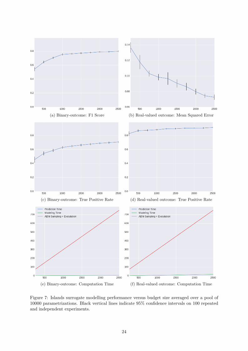
The surrogate’s performances is presented in Figure 7, where the first column of the plotsrefers to the binary outcome setting, while the second one to the real-valued one. The F1-score displays relatively high values even for low training sample sizes (250 and 500) pointingto a good classification performance of the surrogate (see Figure 7a). However, it quicklysaturates, reaching a plateau around 0.8. Conversely, in the real-valued setting, the surrogate’s
18In the real-valued outcome setting our exercise is comparable to those performed in Dosi et al. (2017c), wherethe same distribution and parameters are used in a model of industrial dynamics.
19This choice is motivated by the fact that we need to run the model on the out-of-sample points in order toevaluate the surrogate.
22
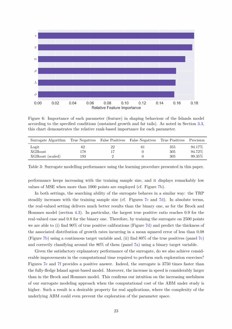
Figure 6: Importance of each parameter (feature) in shaping behaviour of the Islands modelaccording to the specified conditions (sustained growth and fat tails). As noted in Section 3.3,this chart demonstrates the relative rank-based importance for each parameter.
Surrogate Algorithm True Negatives False Positives False Negatives True Positives Precision
Logit 62 22 61 355 94.17%XGBoost 178 17 0 305 94.72%XGBoost (scaled) 193 2 0 305 99.35%
Table 3: Surrogate modelling performance using the learning procedure presented in this paper.
performance keeps increasing with the training sample size, and it displays remarkably lowvalues of MSE when more than 1000 points are employed (cf. Figure 7b).
In both settings, the searching ability of the surrogate behaves in a similar way: the TRPsteadily increases with the training sample size (cf. Figures 7c and 7d). In absolute terms,the real-valued setting delivers much better results than the binary one, as for the Brock andHommes model (section 4.3). In particular, the largest true positive ratio reaches 0.9 for thereal-valued case and 0.8 for the binary one. Therefore, by training the surrogate on 2500 pointswe are able to (i) find 90% of true positive calibrations (Figure 7d) and predict the thickness ofthe associated distribution of growth rates incurring in a mean squared error of less than 0.08(Figure 7b) using a continuous target variable and, (ii) find 80% of the true positives (panel 7c)and correctly classifying around the 80% of them (panel 7a) using a binary target variable.
Given the satisfactory explanatory performance of the surrogate, do we also achieve consid-erable improvements in the computational time required to perform such exploration exercises?Figures 7e and 7f provides a positive answer. Indeed, the surrogate is 3750 times faster thanthe fully-fledge Island agent-based model. Moreover, the increase in speed is considerably largerthan in the Brock and Hommes model. This confirms our intuition on the increasing usefulnessof our surrogate modeling approach when the computational cost of the ABM under study ishigher. Such a result is a desirable property for real applications, where the complexity of theunderlying ABM could even prevent the exploration of the parameter space.
23
(a) Binary-outcome: F1 Score (b) Real-valued outcome: Mean Squared Error
(c) Binary-outcome: True Positive Rate (d) Real-valued outcome: True Positive Rate
(e) Binary-outcome: Computation Time (f) Real-valued outcome: Computation Time
Figure 7: Islands surrogate modelling performance versus budget size averaged over a pool of10000 parametrizations. Black vertical lines indicate 95% confidence intervals on 100 repeatedand independent experiments.
24

5.4 Robustness analysis
We now assess the robustness of our training procedure with respect to different surrogatemodels. More specifically, we compare the XGBoost surrogate employed in the previous analysiswith the simpler and more widely used Logit one. Our comparison exercise is performed in afully stochastic version of the Island agent-based model, where an additional Monte Carlo (MC)is carried out on the seed parameter governing the stochastic terms of the model. As a sneakpreview, we can anticipate that our procedure is pretty robust to different surrogate crus.
We focus on a binary outcome setting (the one delivering worse performances) and weemploy the milder condition that the average growth rate must be positive and sustained, i.e.AGR > 0.5%. In this way, the results can be compared to those obtained in the originalexercise in Fagiolo and Dosi (2003). We set a budget of 500 evaluations of the “true” IslandsABM and run a Monte Carlo exercise of size 100 per parameter combination to generate anMC average of the GDP growth rate that serves as our output variable. Note that this exerciseis more complete that the one performed in the previous sections: here, we develop a surrogatemodel that learns the relationship between parameters and the MC average over their ABMevaluations. Note that this requires many more evaluations of the parameter combination inthe true ABM to converge to the statistic required for the label. In our proposed procedure,an MC average growth rate below 0.5% is labelled “false”, while AGR above 0.5% are labelled“true”. The aim is to learn a surrogate model that accurately classifies parameter combinationsas positive or negative calibrations.
We demonstrate the performance of our active learning approach using two different surro-gates: the XGBoost and the faster, less precise, Logit. The former, employed in the analysescarried out in the previous sections, benefits from increased accuracy in exchange for greatercomputational costs. The latter is a standard statistical model employed regularly for thistype of regression analysis. The performance of these alternative surrogates will be evaluatedaccording to the F1-score while training the surrogate, with the final objective of maximizingthe precision of the resulting models, i.e. the number of true evaluations which are accuratelypredicted as positive before they are evaluated. This is a key point to this exercise becausereal-world use of the proposed approach does not allow us to evaluate all the points in oursample space. Real-world evaluation only provides labels for points that are predicted positiveand the resulting performance can only be measured with regard to the true and false positives,with a preference to maximize the former.
The exercise is performed using the Python BOASM package.20 The algorithm mirror ex-actly the one described in Section 3. The exercise begins by sampling 1000000 points at randomfrom the Islands parameter space. Given the fixed budget of 500 evaluations of the true ABM,for both the XGBoost and Logit, the first surrogate is provided with 35 labelled parameters se-lected at random from the 1000000 points, according to the total-variation sampling procedurein Saltelli et al. (2010). Then, over several rounds, a surrogate will be fit to the labelled param-eters and used to predict a labelling over the 1000000 points. The predicted labels will then beemployed by the proposed procedure to select points that will be added at each round to theset of labelled points. A new surrogate is learned in the subsequent round and the procedure
20See https://github.com/amirsani/BOASM
25

will repeat until the budget of true evaluations has been reached.The proposed procedure results in a comparable precision of 94.17% and 94.72% between
Logit and XGBoost, respectively. The negligible difference between the precision of the two sur-rogates suggests that out training procedure provide satisfying results even when the fast andstandard Logit statistical model is employed. However, when the XGBoost predicted probabili-ties are corrected through the Platt scaling procedure,21 its precision rises to 99.35%. Moreover,scaled XGBoost performs is considerably superior to Logit with regard to true vs. false posi-tives. Considering its higher computation costs and need for hyperparameter optimization inusing the more precise XGBoost surrogate, users might prefer the faster Logit surrogate whenfalse positives are cheap. Nevertheless, our proposed surrogate modelling procedure works wellin both the Logit and XGBoost cases.
6 Discussion and concluding remarks
In this paper, we have proposed a novel approach to the calibration and parameter space explo-ration of agent-based models (ABM), which combines the use of supervised machine learning andintelligent sampling to construct a cheap surrogate meta-model. To the best of our knowledge,this is the first attempt to exploit machine-learning techniques for calibration and explorationin an agent-based framework.
Our machine-learning surrogate approach is different from Kriging, which has been recentlyapplied to ABMs dealing with industrial dynamics (Salle and Yildizoglu, 2014; Dosi et al.,2017c), financial networks (Bargigli et al., 2016) and macroeconomic issues (Dosi et al., 2016,2017b). In particular, apart from the different statistical framework Kriging relies on (it assumesa multivariate Gaussian process), the results it delivers once applied to ABMs may suffer fromthree relevant limitations. First, Kriging is difficult to apply to large scale models, where thenumber of parameters goes beyond 20. This constrains the modeller to introduce additionalprocedures to select, a priori, the subset of parameters to study, while leaving the rest constant(see e.g. Dosi et al., 2016). Second, the machine-learning surrogate approach performs betterin out-of-sample testing: the typical Kriging-based meta-model is tested on 10-20 points withinan extremely large space, while our surrogate is tested on samples with size 10000 in the firstset of exercises and 1000000 points in the last exercise. Finally, the response surfaces generatedby Kriging meta-models suffer from smoothness assumptions that collapse interesting patterns,which cannot be captured by common Gaussianity assumptions. This results in incrediblysmooth and well-behaved surfaces, which may falsely relate parameters and model behaviour.Given the ragged, unsmooth surfaces commonly reported in agent-based models (see e.g. Gilliand Winker, 2003; Fabretti, 2012; Lamperti, 2016), inferring the behaviour of the true ABM onthe basis of the insights produced by Kriging meta-model may results in large errors. Further,even when smooth response surfaces exist, Kringing requires the selection of the correct priorand kernel. Even in state-of-the-art likelihood-free approaches, one must select the correctsufficient statistic and acceptance threshold to provide any value.
21Unlike Logit, which produces accurate probabilities for each of the class labels, probabilities produced by non-parametric algorithms such as XGBoost require scaling. Here, we use Platt Scaling to correct the probabilitiesproduced with XGBoost. For more information, see Platt et al. (1999).
26

Our machine-learning surrogate approach manages all these problems.22 However, the mainadvantage of our methodology remains in its practical usefulness. Indeed, the surrogate canbe learnt at virtually zero computational costs (for research applications) and requires a trivialamount of time to predict areas of the parameter space the modeller should focus on withreasonably good results. Two modelling options are presented, a binary outcome setting anda real-valued one: the first is faster and especially useful when a large number of samples isavailable, while the second has more explanatory power.
Furthermore, the usual trade-off between the quantity of information that needs to be pro-cessed (computational costs) and the surrogate performance improvements is, in practice, ab-sent. Ultimately, the surrogate prediction exercises proposed in this paper take less than aminute to complete, with the majority of computation coming from the time to assess the bud-get of true ABM model evaluations. This means, in practical terms, that the modeller can usean arbitrarily large set of parameter combinations and a relatively small training sample tobuild the surrogate at almost no cost and leverage the resulting meta-model to gain an insighton the dynamics of the parameter space for further exploration using the original ABM.
Finally, an additional relevant result emerges from the iexercises investigated in this paper.The surrogate is much more effective in reducing the relative cost of exploring the propertiesof the model over the parameter space for the “Islands” model, which is more computationallyintensive than the Brock and Hommes. This suggests that the adoption of surrogate meta-modelling allows to achieve increasing computational gains as the complexity of the underlyingmodel increases.
This work is only the first step towards a fully-fledge assessment of the properties of agent-based models employing machine-learning techniques. Such developments are especially im-portant for complex macroeconomic agent-based models (see e.g. Dosi et al., 2010, 2013, 2015,2017a; Popoyan et al., 2017) as they could allow the development of a standardized and robustprocedure for model calibration and validation, thus closing the existing gap with DynamicsStochastic General Equilibrium models (see Fagiolo and Roventini, 2017, for a critical com-parison of ABM and DSGE models). Accordingly, a user-friendly Python surrogate modellinglibrary will also be released for general use.
Acknowledgements
A special thank goes to Antoine Mandel, who constantly engaged in fruitful discussions with the authorsand provided incredibly valuable insights and suggestions. We would also like to thank Daniele Giachini,Mattia Guerini, Matteo Sostero and Balaz Kegl for their comments. Further, we would like to thank allthe participants in seminars and workshops held at Scuola Superiore Sant’Anna (Pisa), the XXI WEHIAconference (Castellon), the XXII CEF conference (Bordeaux), NIPS 2016 ”What If? Inference and Learn-ing of Hypothetical and Counterfactual Interventions in Complex Systems” workshop (Barcelona), CCS2016 conference (Amsterdam) and 2016 Paris-Bielefeld Workshop on Agent-Based Modeling (Paris). FL
22In the current work, we also focus on examples dealing with relatively few parameters. This choice ismotivated by illustrative reasons and the willingness to use well established models whose code is easily replicable.Further, the results from this paper were produced using a relatively common laptop computer with 16 gigabytesof memory and a 2.4Ghz Intel i7 5500 CPU. The application to a large scale model is currently under development.However, the computational parsimony of the algorithm used to construct our surrogates strongly points to theability to deal with much richer parameter spaces.
27

acknowledges financial support from European Union’s FP7 project IMPRESSIONS (G.A. No 603416).AS acknowledges financial support from the H2020 project DOLFINS (G.A. No 640772) and hardwaresupport from NVIDIA Corporation, AdapData SAS and the Grid5000 testbed for this research. ARacknowledges financial support from European UnionâĂŹs FP7 IMPRESSIONS, H2020 DOLFINS andH2020 ISIGROWTH (G.A. No 649186) projects.
ReferencesAlfarano, S., Lux, T., and Wagner, F. (2005). Estimation of agent-based models: The case of an asymmetric
herding model. Computational Economics, 26(1):19–49.
Alfarano, S., Lux, T., and Wagner, F. (2006). Estimation of a simple agent-based model of financial mar-kets: An application to australian stock and foreign exchange data. Physica A: Statistical Mechanics and itsApplications, 370(1):38 – 42.
Amilon, H. (2008). Estimation of an adaptive stock market model with heterogeneous agents. Journal of EmpiricalFinance, 15(2):342 – 362.
An, G. and Wilensky, U. (2009). From artificial life to in silico medicine. In Komosinski, M. and Adamatzky, A.,editors, Artificial Life Models in Software, pages 183–214. Springer London, London.
Anderson, P. W. et al. (1972). More is different. Science, 177(4047):393–396.
Archer, K. J. and Kimes, R. V. (2008). Empirical characterization of random forest variable importance measures.Computational Statistics & Data Analysis, 52(4):2249–2260.
Assenza, T., Gatti, D. D., and Grazzini, J. (2015). Emergent dynamics of a macroeconomic agent based modelwith capital and credit. Journal of Economic Dynamics and Control, 50:5–28.
Banerjee, A. V. (1992). A simple model of herd behavior. The Quarterly Journal of Economics, 107(3):797–817.
Barde, S. (2016a). Direct comparison of agent-based models of herding in financial markets. Journal of EconomicDynamics and Control, 73:329 – 353.
Barde, S. (2016b). A practical, accurate, information criterion for nth order markov processes. ComputationalEconomics, pages 1–44.
Bargigli, L., Riccetti, L., Russo, A., and Gallegati, M. (2016). Network Calibration and Metamodeling of aFinancial Accelerator Agent Based Model. Working papers, economics, Universita degli Studi di Firenze,Dipartimento di Scienze per l’Economia e l’Impresa.
Bergstra, J. and Bengio, Y. (2012). Random search for hyper-parameter optimization. Journal of MachineLearning Research, 13(Feb):281–305.
Booker, A., Dennis, J.E., J., Frank, P., Serafini, D., Torczon, V., and Trosset, M. (1999). A rigorous frameworkfor optimization of expensive functions by surrogates. Structural optimization, 17(1):1–13.
Boswijk, H., Hommes, C., and Manzan, S. (2007). Behavioral heterogeneity in stock prices. Journal of EconomicDynamics and Control, 31(6):1938 – 1970.
Bottazzi, G. and Secchi, A. (2006). Explaining the distribution of firm growth rates. The RAND Journal ofEconomics, 37(2):235–256.
Breiman, L. (2001). Random forests. Machine learning, 45(1):5–32.
Breiman, L., Friedman, J., Stone, C. J., and Olshen, R. A. (1984). Classification and regression trees. CRC press.
Brock, W. A. and Hommes, C. H. (1997). A rational route to randomness. Econometrica, 65(5):1059–1095.
Brock, W. A. and Hommes, C. H. (1998). Heterogeneous beliefs and routes to chaos in a simple asset pricingmodel. Journal of Economic Dynamics and Control, 22(8–9):1235 – 1274.
Brown, D. G., Page, S., Riolo, R., Zellner, M., and Rand, W. (2005). Path dependence and the validation ofagent-based spatial models of land use. International Journal of Geographical Information Science, 19(2):153–174.
28
Caiani, A., Godin, A., Caverzasi, E., Gallegati, M., Kinsella, S., and Stiglitz, J. E. (2016). Agent based-stockflow consistent macroeconomics: Towards a benchmark model. Journal of Economic Dynamics and Control,69:375–408.
Carley, K. M., Fridsma, D. B., Casman, E., Yahja, A., Altman, N., Chen, L.-C., Kaminsky, B., and Nave,D. (2006). Biowar: scalable agent-based model of bioattacks. IEEE Transactions on Systems, Man, andCybernetics-Part A: Systems and Humans, 36(2):252–265.
Castaldi, C. and Dosi, G. (2009). The patterns of output growth of firms and countries: Scale invariances andscale specificities. Empirical Economics, 37(3):475–495.
Chen, S.-H., Chang, C.-L., and Du, Y.-R. (2012). Agent-based economic models and econometrics. The KnowledgeEngineering Review, 27:187–219.
Chen, T. and Guestrin, C. (2016). Xgboost: A scalable tree boosting system. In Proceedings of the 22Nd ACMSIGKDD International Conference on Knowledge Discovery and Data Mining, pages 785–794. ACM.
Chiarella, C., Iori, G., and Perello, J. (2009). The impact of heterogeneous trading rules on the limit order bookand order flows. Journal of Economic Dynamics and Control, 33(3):525–537.
Ciresan, D. C., Giusti, A., Gambardella, L. M., and Schmidhuber, J. (2013). Mitosis detection in breast cancerhistology images with deep neural networks. In International Conference on Medical Image Computing andComputer-assisted Intervention, pages 411–418. Springer.
Claesen, M., Simm, J., Popovic, D., Moreau, Y., and De Moor, B. (2014). Easy hyperparameter search usingoptunity. arXiv preprint arXiv:1412.1114.
Conti, S. and O’Hagan, A. (2010). Bayesian emulation of complex multi-output and dynamic computer models.Journal of statistical planning and inference, 140(3):640–651.
Dawid, H., Gemkow, S., Harting, P., Van der Hoog, S., and Neugart, M. (2014a). Agent-based macroeconomicmodeling and policy analysis: the eurace@ unibi model. Technical report, Bielefeld Working Papers in Eco-nomics and Management.
Dawid, H., Harting, P., and Neugart, M. (2014b). Economic convergence: Policy implications from a heteroge-neous agent model. Journal of Economic Dynamics and Control, 44:54–80.
De Marchi, S. (2005). Computational and mathematical modeling in the social sciences. Cambridge UniversityPress.
Dosi, G. (1988). Sources, procedures and microeconomic effects of innovation. Journal of Economic Literature,26:126–71.
Dosi, G., Fagiolo, G., Napoletano, M., and Roventini, A. (2013). Income distribution, credit and fiscal policiesin an agent-based Keynesian model. Journal of Economic Dynamics and Control, 37(8):1598–1625.
Dosi, G., Fagiolo, G., Napoletano, M., Roventini, A., and Treibich, T. (2015). Fiscal and monetary policies incomplex evolving economies. Journal of Economic Dynamics and Control, 52(C):166–189.
Dosi, G., Fagiolo, G., and Roventini, A. (2010). Schumpeter meeting Keynes: A policy-friendly model of endoge-nous growth and business cycles. Journal of Economic Dynamics and Control, 34(9):1748–1767.
Dosi, G., Pereira, M., Roventini, A., and Virgillito, M. (2017a). When more flexibility yields more fragility:The microfoundations of keynesian aggregate unemployment. Journal of Economic Dynamics and Control,forthcoming.
Dosi, G., Pereira, M., Roventini, A., and Virgillito, M. E. (2016). The Effects of Labour Market Reforms uponUnemployment and Income Inequalities: an Agent Based Model. LEM Working Papers Series 2016-27, ScuolaSuperiore Sant’Anna.
Dosi, G., Pereira, M., Roventini, A., and Virgillito, M. E. (2017b). Causes and consequences of hysteresis:Aggregate demand, productivity and employment. LEM Working Papers Series 2017-07, Scuola SuperioreSant’Anna.
Dosi, G., Pereira, M. C., and Virgillito, M. E. (2017c). On the robustness of the fat-tailed distribution of firmgrowth rates: a global sensitivity analysis. Journal of Economic Interaction and Coordination, pages 1–21.
29
Effken, J. A., Carley, K. M., Lee, J.-S., Brewer, B. B., and Verran, J. A. (2012). Simulating nursing unitperformance with orgahead: strengths and challenges. Computers, informatics, nursing: CIN, 30(11):620.
Fabretti, A. (2012). On the problem of calibrating an agent based model for financial markets. Journal ofEconomic Interaction and Coordination, 8(2):277–293.
Fagiolo, G., Birchenhall, C., and Windrum, P. (2007). Empirical validation in agent-based models: Introductionto the special issue. Computational Economics, 30(3):189–194.
Fagiolo, G. and Dosi, G. (2003). Exploitation, exploration and innovation in a model of endogenous growth withlocally interacting agents. Structural Change and Economic Dynamics, 14(3):237–273.
Fagiolo, G., Napoletano, M., and Roventini, A. (2008). Are output growth-rate distributions fat-tailed? someevidence from oecd countries. Journal of Applied Econometrics, 23(5):639–669.
Fagiolo, G. and Roventini, A. (2012). Macroeconomic policy in dsge and agent-based models. Revue de l’OFCE,124:67–116.
Fagiolo, G. and Roventini, A. (2017). Macroeconomic policy in dsge and agent-based models redux: Newdevelopments and challenges ahead. Journal of Artificial Societies and Social Simulation, 20(1).
Feurer, M., Klein, A., Eggensperger, K., Springenberg, J., Blum, M., and Hutter, F. (2015). Efficient and robustautomated machine learning. In Advances in Neural Information Processing Systems, pages 2962–2970.
Franke, R. (2009). Applying the method of simulated moments to estimate a small agent-based asset pricingmodel. Journal of Empirical Finance, 16(5):804 – 815.
Franke, R. and Westerhoff, F. (2012). Structural stochastic volatility in asset pricing dynamics: Estimation andmodel contest. Journal of Economic Dynamics and Control, 36(8):1193–1211.
Freund, Y. (1990). Boosting a weak learning algorithm by majority. In COLT, volume 90, pages 202–216.
Freund, Y., Schapire, R. E., et al. (1996). Experiments with a new boosting algorithm. In Icml, volume 96, pages148–156.
Gallegati, M. and Kirman, A. (2012). Reconstructing economics. Complexity Economics, 1(1):5–31.
Gilli, M. and Winker, P. (2003). A global optimization heuristic for estimating agent based models. ComputationalStatistics & Data Analysis, 42(3):299 – 312. Computational Ecomometrics.
Goldberg, A. B., Zhu, X., Furger, A., and Xu, J.-M. (2011). Oasis: Online active semi-supervised learning. InAAAI.
Grazzini, J. (2012). Analysis of the emergent properties: Stationarity and ergodicity. Journal of ArtificialSocieties and Social Simulation, 15(2):7.
Grazzini, J. and Richiardi, M. (2015). Estimation of ergodic agent-based models by simulated minimum distance.Journal of Economic Dynamics and Control, 51:148 – 165.
Grazzini, J., Richiardi, M. G., and Tsionas, M. (2017). Bayesian estimation of agent-based models. Journal ofEconomic Dynamics and Control, 77:26 – 47.
Grimm, V. and Railsback, S. F. (2013). Individual-based modeling and ecology. Princeton university press.
Guerini, M. and Moneta, A. (2016). A Method for Agent-Based Models Validation. LEM Papers Series 2016/16,Laboratory of Economics and Management (LEM), Sant’Anna School of Advanced Studies, Pisa, Italy.
Herlands, W., Wilson, A., Nickisch, H., Flaxman, S., Neill, D., Van Panhuis, W., and Xing, E. (2015). Scalablegaussian processes for characterizing multidimensional change surfaces. arXiv preprint arXiv:1511.04408.
Ilachinski, A. (1997). Irreducible semi-autonomous adaptive combat (isaac): An artificial-life approach to landwarfare. Technical report, DTIC Document.
Kukacka, J. and Barunik, J. (2016). Estimation of financial agent-based models with simulated maximumlikelihood. IES Working Paper 7/2016, Charles University of Prague.
Lamperti, F. (2016). Empirical Validation of Simulated Models through the GSL-div: an Illustrative Application.LEM Papers Series 2016/18, Laboratory of Economics and Management (LEM), Sant’Anna School of AdvancedStudies, Pisa, Italy.
30

Lamperti, F. (2017). An information theoretic criterion for empirical validation of simulation models. Economet-rics and Statistics, forthcoming.
Lamperti, F., Dosi, G., Napoletano, M., Roventini, A., and Sapio, A. (2017). Faraway, so close: coupled climateand economic dynamics in an agent based integrated assessment model. Lem working papers series, ScuolaSuperiore Sant’Anna.
Lamperti, F. and Mattei, C. E. (2016). Going Up and Down: Rethinking the Empirics of Growth in theDeveloping and Newly Industrialized World. LEM Papers Series 2016/01, Laboratory of Economics andManagement (LEM), Sant’Anna School of Advanced Studies, Pisa, Italy.
Leal, S. J., Napoletano, M., Roventini, A., and Fagiolo, G. (2014). Rock around the clock: an agent-based modelof low-and high-frequency trading. Journal of Evolutionary Economics, pages 1–28.
Lee, J.-S., Filatova, T., Ligmann-Zielinska, A., Hassani-Mahmooei, B., Stonedahl, F., Lorscheid, I., Voinov, A.,Polhill, J. G., Sun, Z., and Parker, D. C. (2015). The complexities of agent-based modeling output analysis.Journal of Artificial Societies and Social Simulation, 18(4):4.
Li, X., Engelbrecht, A., and Epitropakis, M. G. (2013). Benchmark functions for cec’2013 special session andcompetition on niching methods for multimodal function optimization. RMIT University, Evolutionary Com-putation and Machine Learning Group, Australia, Tech. Rep.
Louppe, G., Wehenkel, L., Sutera, A., and Geurts, P. (2013). Understanding variable importances in forests ofrandomized trees. In Advances in neural information processing systems, pages 431–439.
Lux, T. and Marchesi, M. (2000). Volatility clustering in financial markets: a microsimulation of interactingagents. International journal of theoretical and applied finance, 3(04):675–702.
Macy, M. W. and Willer, R. (2002). From factors to actors: Computational sociology and agent-based modeling.Annual review of sociology, pages 143–166.
Marks, R. E. (2013). Validation and model selection: Three similarity measures compared. Complexity Economics,2(1):41–61.
Morokoff, W. J. and Caflisch, R. E. (1994). Quasi-random sequences and their discrepancies. SIAM Journal onScientific Computing, 15(6):1251–1279.
Moss, S. (2008). Alternative approaches to the empirical validation of agent-based models. Journal of ArtificialSocieties and Social Simulation, 11(1):5.
Petrovic, S., Osborne, M., and Lavrenko, V. (2011). Rt to win! predicting message propagation in twitter.ICWSM, 11:586–589.
Platt, J. et al. (1999). Probabilistic outputs for support vector machines and comparisons to regularized likelihoodmethods. Advances in large margin classifiers, 10(3):61–74.
Popoyan, L., Napoletano, M., and Roventini, A. (2017). Taming Macroeconomic Instability: Monetary and MacroPrudential Policy Interactions in an Agent-Based Model. Journal of Economic Behavior & Organization,134:117–140.
Rasmussen, C. E. and Williams, C. K. I. (2006). Gaussian processes for machine learning. MIT Press.
Recchioni, M. C., Tedeschi, G., and Gallegati, M. (2015). A calibration procedure for analyzing stock pricedynamics in an agent-based framework. Journal of Economic Dynamics and Control, 60:1 – 25.
Ross, S., Gordon, G. J., and Bagnell, D. (2011). A reduction of imitation learning and structured prediction tono-regret online learning. In AISTATS, volume 1(2), page 6.
Ryabko, D. (2016). Things bayes can’t do. In International Conference on Algorithmic Learning Theory, pages253–260. Springer.
Salle, I. and Yildizoglu, M. (2014). Efficient Sampling and Meta-Modeling for Computational Economic Models.Computational Economics, 44(4):507–536.
Saltelli, A., Annoni, P., Azzini, I., Campolongo, F., Ratto, M., and Tarantola, S. (2010). Variance basedsensitivity analysis of model output. design and estimator for the total sensitivity index. Computer PhysicsCommunications, 181(2):259–270.
31

Settles, B. (2010). Active learning literature survey. Technical Report 55-66, University of Wisconsin, Madison.
Squazzoni, F. (2010). The impact of agent-based models in the social sciences after 15 years of incursions. Historyof Economic Ideas, pages 197–233.
Subbotin, M. T. (1923). On the law of frequency of error. Matematicheskii Sbornik, 31(2):296–301.
ten Broeke, G., van Voorn, G., and Ligtenberg, A. (2016). Which sensitivity analysis method should i use for myagent-based model? Journal of Artificial Societies & Social Simulation, 19(1).
Tesfatsion, L. and Judd, K. L. (2006). Handbook of computational economics: agent-based computational eco-nomics, volume 2. Elsevier.
Thiele, J. C., Kurth, W., and Grimm, V. (2014). Facilitating parameter estimation and sensitivity analysis ofagent-based models: A cookbook using netlogo and r. Journal of Artificial Societies and Social Simulation,17(3):11.
van der Hoog, S. (2016). Deep Learning in Agent-Based Models: A Prospectus. Technical report, Faculty ofBusiness Administration and Economics, Bielefeld University.
Van Rijsbergen, C. (1979). Information Retrieval. London: Butterworths.
Weeks, M. (1995). Circumventing the curse of dimensionality in applied work using computer intensive methods.The Economic Journal, 105(429):520–530.
Wilson, A. G., Dann, C., and Nickisch, H. (2015). Thoughts on massively scalable gaussian processes. arXivpreprint arXiv:1511.01870.
Winker, P., Gilli, M., and Jeleskovic, V. (2007). An objective function for simulation based inference on exchangerate data. Journal of Economic Interaction and Coordination, 2(2):125–145.
Wolpert, D. H. (2002). The supervised learning no-free-lunch theorems. In Soft Computing and Industry, pages25–42. Springer.
Wong, K.-C. (2015). Evolutionary multimodal optimization: A short survey. arXiv preprint arXiv:1508.00457.
Zhu, X. (2005). Semi-supervised learning literature survey. Technical report, University of Wisconsin-Madison.
32