aggregate dynamics in a large virtual economy: … dynamics in a large virtual economy: prices and...
TRANSCRIPT

Aggregate Dynamics in a Large Virtual Economy:
Prices and Real Activity in Team Fortress 2∗
Matt Baumer† Curtis Kephart‡
University of California Santa Cruz
March 23, 2015
Abstract
We examine economic activity in a large virtual economy which was designed to allow de-centralized barter as the sole exchange institution. We find that a small subset of goods emergesendogenously which act of media of exchange. Our analysis includes estimation of spot exchangerates between these numerous money goods and we develop methods which allows us to priceall goods and track inflation. We then calculate nominal growth and its components. We findthat per-captita real wealth is an increasing component of nominal growth. Separately, we findevidence of a certain form of nominal price ridigity– the price of an item commonly priced in aparticular money good tends to move with the exchange rate of that money good. We also findthat announcements made by the economic planners can induce speculation leading to localizedasset price bubbles.
Keywords: Virtual economy, barter system, national income accounting, wealth measurement,price level, inflation.
JEL Codes: E01 E31 P44
1 Introduction
The object of our study is the virtual economy of Team Fortress 2 (TF2) developed and overseen
by Valve Software. This economy and others like it hold great potential for researchers: millions
of users engaging in billions of economic transactions involving thousands of different types of
goods; the game designers are near-omnipotent social planners able to create and destroy goods
∗The authors would like to thank the valuable assistance provided to us by Valve Corporation, including BrandonReinhart, Kyle Davis, and particularly Kristian Miller for his boundless support and deep insight into the Valvevirtual economy. The research was partially funded by Valve Corporation, the University of California Santa Cruz,and LEEPS Lab. Valve Corporation additionally provided technology grants and access to anonymized proprietarydata. The authors have agreements in place that entitle Valve Corporation to review our work before it beingsubmitted for publication. The authors would also like to thank Danny Oberhaus at Statistics New Zealand andAnya Stockburger at the Bureau of Labor Statistics for offering their expertise in the development of our price index.Matthew Jee, Sergio Ortiz, and Matthew Browne provided excellent computer programming support.†Economics Department, University of California Santa Cruz, CA 95064, [email protected]‡Economics Department, University of California Santa Cruz, CA 95064, [email protected]

and implement policy at will; and they gather essentially complete micro data that enables precise
construction of macro variables. These economies have a close parallel to “real-world” markets
which have recently seen an explosion of detailed high frequency scanner data. But record keeping
is still nowhere near as complete as found in virtual economies like that of TF2.
The TF2 economy has some features that are unusual, even for a virtual economy. There is
no explicit currency good, and trading occurs exclusively through decentralized barter. Goods are
homogeneous and of known quality (i.e. there are no “lemons” as in Akerlof (1970)). Items are
also durable and do not depreciate due to “wear and tear” in the way that a physical item would.
Another issue likely important is that items are indivisible and can only be exchanged in discrete
quantities (e.g. it is impossible to trade half of a common currency item, the treasure key, as keys
are not capable of being split). There is also a significant amount of activity that is due to a very
small number of very active individuals, which we will refer to as “high net worth individuals”
(HNWIs). These quirks will be leveraged in future papers to discuss the issue of the spontaneous
emergence of money, the emergence of trade intermediaries, and information brokerage services by
applying concepts from network theory to map the interactions between different types of user.
Our approach advances ideas presented in Castronova et al. (2009) and Castronova (2008) by
implementing more rigorous economic indicators of aggregate economic behavior in a large virtual
economy. But there are also some crucial differences in our work: Castronova studies Everquest
II, a economy with explicit currency (gold pieces) and in-game posted-price markets available to
the users, thus trade in that environment would not be considered barter or decentralized in any
sense. Our work also more directly adheres to methodology commonly used in modern empirical
economic techniques.
Everquest II and TF2 are far from the only such examples of large virtual worlds with economic
activity: “Second Life” is an entire virtual world, complete with in-game real estate, stores, jobs,
and of course other people. “World of Warcraft” has players fight monsters and each other with
the hope of saving the realm from the great evil that threatens it and has players engaging in
money-mediated trade with each other to facilitate this end.
Even the NYSE has made its operations completely digital. Traders physically standing on the
trading floor on Wall Street are in fact conducting all of their business through computer servers
located in Mahwah, New Jersey. Stock traders are now similarly employed in the business of
2

exchanging zeroes and ones in a computer database, albeit with higher stakes and a much greater
degree of sophistication. The NYSE and its affiliated traders have had almost 200 years to develop
their institutions; who knows what commerce in virtual economies will look like once it matures.
2 Research Questions
Q1: What is the trend in real growth per-capita and how can we explain this trend?
Our primary goal is a basic macroeconomic characterization of this large virtual economy. We
will examine the dynamics of real growth and explain what are the economic causes of dynamics.
We also will perform a decomposition of nominal growth into its constituent components: growth
of the price level, real growth, and population growth.
Q2: How do macroeconomic aggregates (e.g. the price level) respond to macro-level shocks?
An appealing consequence of the complete nature of our dataset is the ability for us to pinpoint
precisely what might be causing, for example, bouts of inflation or deflation. There are also
numerous exogenous policy changes and events that appear to have influenced this economy and
can be detected in our indicators.
Q3: How do markets for individual items respond to micro-level shocks?
A quirk of this environment is that there are numerous unexpected events that can be taken
as exogenous by market participants. For example, a number of cosmetic items were suddenly
“retired”, meaning they were removed from the store and new items of these types could no longer
be acquired, fixing their number in the economy. We might expect this intervention to increase
prices – essentially a negative shock to supply – but it is also possible that market participants’
speculation “overshoots” the new (post-announcement) fundamental value.
3 Environment and Data
Team Fortress 2 is a competitive multiplayer first-person-shooter game which has two teams of
typically 6 to 10 combatants vying for supremacy. Winning could result from (depending on the
game mode) killing enough of your opponents (but don’t worry, death is only temporary!), capturing
3
0
200,000
400,000
600,000
2011 2012 2013 2014Date
Pla
yers
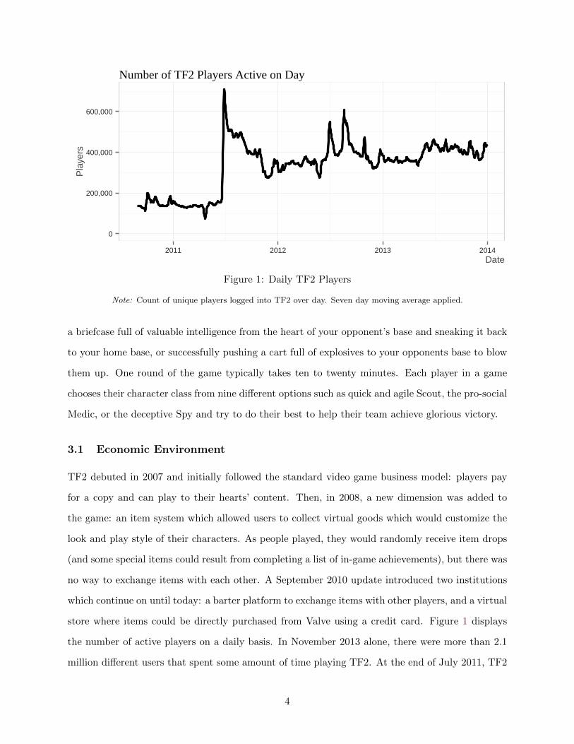
Number of TF2 Players Active on Day
Figure 1: Daily TF2 Players
Note: Count of unique players logged into TF2 over day. Seven day moving average applied.
a briefcase full of valuable intelligence from the heart of your opponent’s base and sneaking it back
to your home base, or successfully pushing a cart full of explosives to your opponents base to blow
them up. One round of the game typically takes ten to twenty minutes. Each player in a game
chooses their character class from nine different options such as quick and agile Scout, the pro-social
Medic, or the deceptive Spy and try to do their best to help their team achieve glorious victory.
3.1 Economic Environment
TF2 debuted in 2007 and initially followed the standard video game business model: players pay
for a copy and can play to their hearts’ content. Then, in 2008, a new dimension was added to
the game: an item system which allowed users to collect virtual goods which would customize the
look and play style of their characters. As people played, they would randomly receive item drops
(and some special items could result from completing a list of in-game achievements), but there was
no way to exchange items with each other. A September 2010 update introduced two institutions
which continue on until today: a barter platform to exchange items with other players, and a virtual
store where items could be directly purchased from Valve using a credit card. Figure 1 displays
the number of active players on a daily basis. In November 2013 alone, there were more than 2.1
million different users that spent some amount of time playing TF2. At the end of July 2011, TF2
4

went “free-to-play” (F2P), removing the requirement to purchase a game license before people are
allowed to play, at which point the game generated revenue only by selling in-game items on the
official store.
An item in the context of the Valve marketplace as any virtual good that can be stored in a
players inventory (henceforth referred to as a “backpack”) and be traded. These may include TF2
items, installation licenses for other games on Valve’s digital distribution platform called Steam,
and items from games other than TF2 on the Steam platform. Backpacks have finite space, but
the capacity is large enough (300 item slots) that most users are unlikely feel this constraint. As
well, there are “backpack expanders” that can be purchased from Valve for $.99 which loosen this
constraint by granting an additional 100 item slots.
The process of successfully completing a trade is as follows: Find a trading partner through
communication channels that can be internal or external to TF2, add them to your contact list,
request a trade session, arrange an exchange in that session which makes both parties happy, and
then execute the trade after multiple layers of confirmation. This is a quite inconvenient system for
the market participants, but it represents an opportunity for inquiring economists to study actual
human behavior in an environment in which we are theoretically well versed. It is important to
point out that the economy by construction was designed to support only barter.
Our sample consists of a full log of all transactions occurring between 9 August 2011 and 31
May 2013, a 661 day interval. There were more than 70 million barter transactions, which averages
out to more than 100,000 trades per day or over one trade per second. This is the primary source
of the data set which we will use to do the following analysis. Across these 70 million individual
transactions, over 300 million virtual items changed hands. There were 4,267,832 unique traders
participating in the barter market, with the median trader conducting 4 exchanges, and with
approximately one third of traders exchanging ten or more items over the sample period. Some
traders participated in a large number of trades; the top ten accounts by trade count each conducted
over 150,000 barter transactions.1
The Team Fortress 2 trading environment represents the largest dataset of a barter exchange
1User Privacy: In order to protect the privacy of individuals involved in the TF2 Economy, user identities werewere anonymized, timestamps masked, and any data containing unique user identifiers was held on Valve Corporationmachines. Though the researchers were given access to the full log of market transactions, all other company suppliedmetrics removed users who marked their Steam backpacks to private.
5

10
1,000
100,000
10 1,000 100,000Number of Trades Conducted by Individual Accounts
Fre
quen
cyTrade Frequency
Figure 2: Histogram of User Trade Frequency
Note: Due to length of tail, top 10% of traders are not visible. Includes trading of non-TF2 game items and “Steam”game licenses. Does not include players who did not trade at least once.
market that we are aware of. This is all the more remarkable since barter markets today tend
to emerge in environments which feature weak institutions and consequently have meager record-
keeping.
Items in TF2 have various types. There are consumables that are used in conjunction with other
items (e.g. a can of paint that can be used on a cosmetic that changes the item’s color palette,
or a name tag that lets the player choose a custom name for their item) and durables which can
be used for as long as the owner wishes and do not undergo any sort of depreciation as a result of
use. All durables have associated class restrictions; some durables can be equipped by any class
and others can only be equipped by one or a few classes.
In addition, each individual item is designated one of a number of different “qualities”, which
serve primary to signal scarcity and characteristics of the item. These include “unique” quality
(which is, counterintuitively, the most common item quality), “unusual” quality (which adds a
custom effect to the item such as flames erupting from the item’s surface and are overall the rarest
and most sought after quality), “strange” quality (which track various statistics for the player when
worn), and a few other qualities which are functionally similar to uniques.
Players can gain items from a number of different sources: random drops from playing (although
6

there is a cap of how many items can be received per time period from this source), direct purchase
from the “Valve store” using real cash, special promotions (e.g. holidays, as a reward for completing
some achievement, or as an incentive for buying another game), trading with other players, by
opening crates which require a key which is then consumed along with the crate, and through a
crafting system introduced in December of 2009.
From observation of the set of items most commonly used as a unit of account on independent
community-created trading posts, there is evidence that the widely accepted commodity currencies
include three denominations of “metals”, “keys”, “Bill’s Hats”, and “Earbuds”. The three different
types of metals in order of increasing value are scrap, reclaimed, and refined. There exists an
in-game system that allows conversion of one denomination into another in either direction at the
rate of 3 lower valued to 1 of the next higher valued. For example, anyone can convert 3 scrap
metals into 1 reclaimed, then combine that reclaimed with 2 more reclaimed to create a refined,
then break that refined back into 3 reclaimed. There is no cost associated with these conversions
beyond the time it takes to perform them.
Metals result from scrapping (deleting) weapons from your backpack and are used in combina-
tion with other metals and items to create new items via defined recipes. Keys only come from
store purchases and may be used to open crates that contain new items with various probabilities.
Crates are analogous to raffle tickets; if you pay the cost of one key to open a crate, you will most
likely get an item worth somewhat less than the key but there is a small chance to get a very
valuable item worth much more.
Metals and keys are created and consumed regularly. Bill’s Hats and Earbuds, in contrast,
entered the market as promotional items given away in the past and can no longer be found or
purchased directly from Valve. Their supply is bounded by the current number in existence and
slowly shrinks due to people quitting the game or deleting them.
Once a player is in possession of an item, they will not lose it unless they either trade, delete, or
consume the item in the case of consumables. At the end of 2012, the ability for players to sell items
directly to other players for Valve store credit in an official centralized posted-price marketplace
was added. This store credit is denominated in the player’s local currency and is redeemable for
TF2 items purchased from the Valve store as well as the purchase of licenses for other games from
Valve’s digital distribution platform called “Steam”.
7

This demonstrates an important distinction between this economy and the physical world;
in order to produce a good there are raw materials that necessarily must be consumed due to
conservation of mass. But the production of an additional good in this virtual economy requires
no more than a additional line saved to a database. There is still technically an upper bound on
how many items can exist, but for practical purposes this horizon is infinite and the marginal cost
of production of these goods is practically zero for Valve.
Another distinction between this environment and physical economies comes from the nature
of consumption. Most real goods are actually consumed at some rate and once they are used up,
are no longer usable again. This does not happen in TF2. Most consumption is of goods which are
perfectly durable (with the exception of tools, but tools either result in or modify durables). We
can then think of the size of this economy as being the aggregate value of the stock of durables and
tools.
3.2 Data
Much of our data takes the form of logs documenting barter transactions of virtual items between
two users. These are lists of transactions linked to users and the individual items associated with
the trade. These data were supplied to us via a half terabyte sized relational database from which
we generated observations in the form of Table 1. Each row in the transactions log represents
the movement of a single item and is associated with a unique trade identifier, two unique player
identifiers (one for the sender of the item and one for the recipient), a unique item-level identifier
which no two items share (AssetID), and an identifier for the specific item type which identical
items would share with each other (EconAssetClass). For example, if a player possesses two unique
quality “Bill’s Hats” that are otherwise identical, they would share an EconAssetClass but also each
will be associated with unique AssetID that represents the specific individual item. Technically,
when an item is traded its old AssetID is removed from the originating user’s inventory and a
new one is created for the user receiving it. Thus, we can track both individual items as well as
individual classes of items, defined as items which share a type and quality which makes them
functionally identical.
We present as an example Table 1. By looking at trade IDs, we can classify each individual
trade into categories such as simple monetary trades or simple barter trades, as will be discussed
8

Table 1: Example data snippet
TradeID PartyA PartyB Time AppID AssetID NewAssetID Origin EconAssetClass1 1203 1876 1351926000 440 38818 41361 1 1002 4256 172 1351927010 440 39425 41362 0 1949212 4256 172 1351927010 440 41359 41363 1 1585353 993 8384 1351928320 440 41339 41364 0 207
in detail later. Party A and B allow us to track the trading behavior of individual traders and
the AssetID and NewAssetID let us track the movements of individual items as they pass from
user to user. Origin indicates which user is the recipient of the item transfer and EconAssetClass
is the identifier which lets us determine the specific item type that was traded. In this fabricated
example, the first trade was a one-way exchange where a player with ID number 1876 gave an item
to another player with ID number 1203 and received nothing in return. The item that was given
away was of type 100. The next trade involved the player 4256 giving an item of type 194921 to
player 172 and receiving an item of type 158535 in exchange.
4 Estimating Prices from Barter Data
Our approach to generating prices for individual items is to define one good among the emergent
currencies to be our numeraire, calculate spot exchange rates between the other currencies and our
numeraire, and convert goods exchanged for those alternative currencies into the corresponding
value of the numeraire. This approach gives us price estimates which allow for direct value compar-
isons between all items. We also generate statistics for each item including daily turnover, number
of trades, and stocks.
The question of how to define which goods are used as “currencies” and which are not is
not a trivial one, but this discussion is not something we shall delve into in this paper.2 Since
the different metals can be converted costlessly into each other in either direction at the rates
mentioned previously, we convert all price observations involving metal into the equivalent value in
terms of refined metal.
From all of the goods used as commodity currencies, we choose keys to be the numeraire. Keys
2In upcoming work we will rigorously identify goods that appear to be the most “money-like” based on theircharacteristics in the data, but for this paper we will simply take money goods for granted and assign currency statusto those items which are used as a unit of account in the major community-run pricing resources.
9

FX - Money for Money
SM - Simple Monetary
SM.Keys - Simple Monetary with Keys
SM.Mix - Simple Monetary with Mix
Basket on Side 1 Basket on Side 2
SB - Simple Barter
OW - One-Way
EE - Everything Else
EE.SM - Simple Monetary in EE
EE - All other trades
All Money Goodsof any type or mix
All Money Goodsof any type or mix
All Key(s) Non Money Good(s)of one type
All Money Goodsof any type or mix
Non Money Good(s)of one type
All Money Goodsof any type or mix
Non Money Good(s)of one type
Non Money Good(s)of one type
Any Item(s) Empty
Money Goodsof any type or mix
Non Money Good(s)of one type
Figure 3: List of Trade Classification Types.
were selected because they appear to have the most stable value, likely due to the fact that their
supply is allowed to expand as well as contract and the price is anchored to the dollar since keys
can only be produced the economy through direct purchases from the Valve store at a price of
$2.49 per key. The other potential currency goods either were introduced later on (Bill’s Hats and
Earbuds) or displayed rapid expansion of supply (faster than the growth of population) causing
instability in estimated prices.
We define a simple monetary (SM) trade observation as a single exchange involving a single
non-currency item type and any commodity currency items. In order to use SM trades to estimate
prices that are comparable to each other, prices need to be measured in a common unit, which we
refer to as “synthetic keys”. A synthetic key price is the equivalent key-value of a good perhaps
exchanged for non-key money(s). We calculate daily exchange rates between different types of
money items by looking at the subset of trades that are money for money (FX), which are defined
as trades which have only money goods on both sides. See Figure 3 for a complete classification of
all possible trade types.
By looking at these FX trades, we generate daily inter-money exchange rates as follows. Define
10
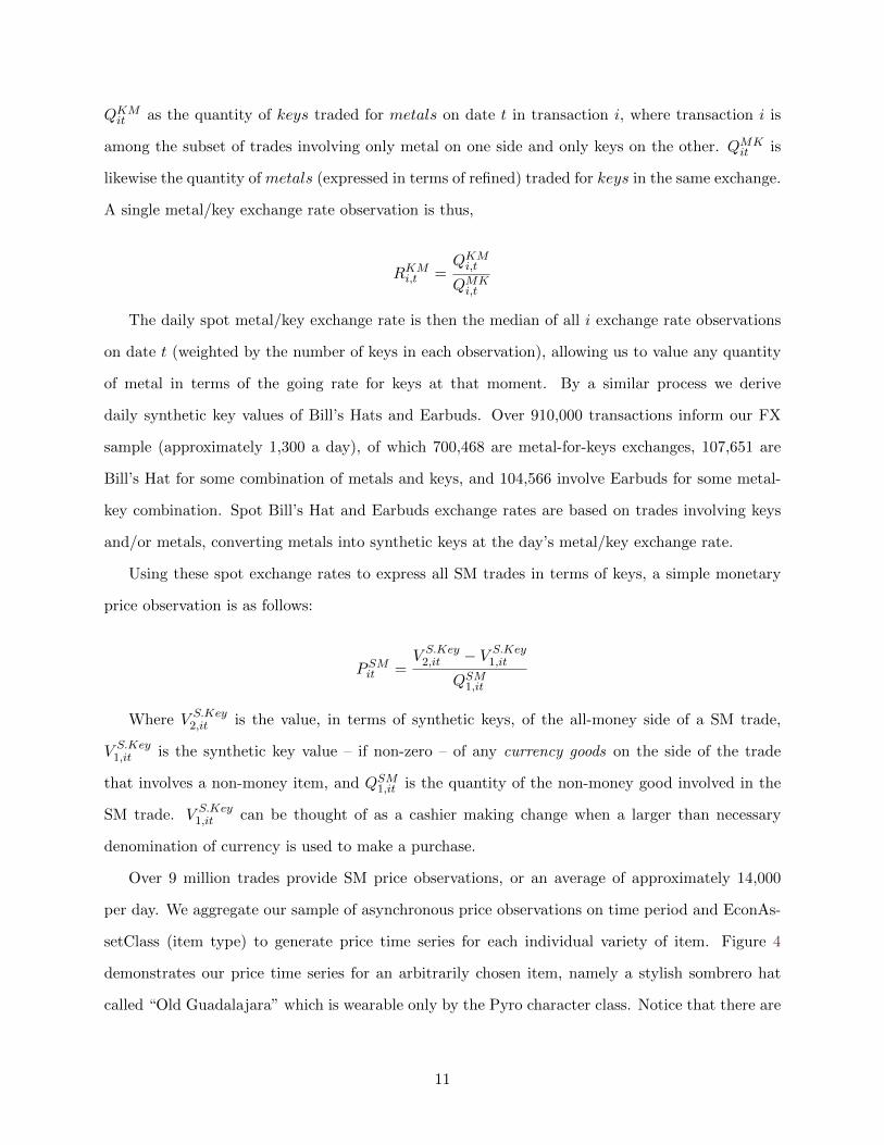
QKMit as the quantity of keys traded for metals on date t in transaction i, where transaction i is
among the subset of trades involving only metal on one side and only keys on the other. QMKit is
likewise the quantity of metals (expressed in terms of refined) traded for keys in the same exchange.
A single metal/key exchange rate observation is thus,
RKMi,t =QKMi,t
QMKi,t
The daily spot metal/key exchange rate is then the median of all i exchange rate observations
on date t (weighted by the number of keys in each observation), allowing us to value any quantity
of metal in terms of the going rate for keys at that moment. By a similar process we derive
daily synthetic key values of Bill’s Hats and Earbuds. Over 910,000 transactions inform our FX
sample (approximately 1,300 a day), of which 700,468 are metal-for-keys exchanges, 107,651 are
Bill’s Hat for some combination of metals and keys, and 104,566 involve Earbuds for some metal-
key combination. Spot Bill’s Hat and Earbuds exchange rates are based on trades involving keys
and/or metals, converting metals into synthetic keys at the day’s metal/key exchange rate.
Using these spot exchange rates to express all SM trades in terms of keys, a simple monetary
price observation is as follows:
PSMit =V S.Key2,it − V S.Key
1,it
QSM1,it
Where V S.Key2,it is the value, in terms of synthetic keys, of the all-money side of a SM trade,
V S.Key1,it is the synthetic key value – if non-zero – of any currency goods on the side of the trade
that involves a non-money item, and QSM1,it is the quantity of the non-money good involved in the
SM trade. V S.Key1,it can be thought of as a cashier making change when a larger than necessary
denomination of currency is used to make a purchase.
Over 9 million trades provide SM price observations, or an average of approximately 14,000
per day. We aggregate our sample of asynchronous price observations on time period and EconAs-
setClass (item type) to generate price time series for each individual variety of item. Figure 4
demonstrates our price time series for an arbitrarily chosen item, namely a stylish sombrero hat
called “Old Guadalajara” which is wearable only by the Pyro character class. Notice that there are
11

Figure 4: Price time series and meta data.
Note: A typical individual item price time series. Scatter points reflect individual transactions and their impliedvaluation. Multicolored lines reflect various temporal aggregate methods deriving daily prices.
discrete bands above and below the price trend line; this is a consequence of the indivisibility of the
currency goods. Prior to October 2012, these bands are .1-.15 keys away from each other, which
would correspond to the value of one reclaimed metal at contemporary market exchange rates.
An additional 8.5 million trades offer Simple Barter (SB) item value observations as well –
trades that involve only two non-money items. However, we only use SM price observations and
did not incorporate SB prices because they appear to have a more complicated valuation method
than SM trades. It appears that when traders meet, if the buyer of the specific item does not or
can not pay in currency items, they must pay a premium with their non-money items, meaning
the trade won’t be balanced in terms of value. This would simply introduce mean-zero noise to
valuations if we assume that all items are equally sought after by barter traders. But if some items
were relatively more sought after than other for barter exchange, there would be some item-specific
fixed term that would need to be controlled for. We therefore choose to exclude SB observations
from our price estimations as we determined that the number of SM trades is sufficiently large that
our estimation process will be precise.
Our temporal aggregation approach assumes that each item at every moment possesses an
underlying “fundamental market valuation” based on its characteristics and relevant market condi-
tions. We then take each individual price observation as a noisy signal for that item’s contemporary
12

fundamental value. That is, we assume SM price observations are drawn from their true values,
plus some error process. It is worth mentioning that some items appear to have reasonably complex
profiles, such as bimodality in price, which we take as further evidence of the economic significance
of currency indivisibility.
To estimate the price of a given item on a given day, we start with a seven day window centered
on that day and collect all observed SM transactions involving that item. We then clean out
observations beyond the 1st and 9th price deciles as there are a large number of outliers which,
for thinly traded items, can lead to a large amount of volatility. To estimate prices using a rolling
average, we then apply a weighting function to these price observations based on temporal distance
from the day in question and widen the time window beyond one day if necessary.3
A distinguishing characteristic of this environment is the constant addition of new types of
items that players can buy or find. This methodology involves taking observed transactions around
a given day and using those to estimate spot prices. This approach is not ideal for pricing items
soon after their introduction because there will be relatively few observations. To mitigate this
issue, we also develop a hedonic pricing model that imputes prices of items based on observable
characteristics and supplement price estimates directly as above with estimates from this hedonic
model for use in our price index. This hedonic model will be discussed further in the next section.
5 Methods
5.1 Market Capitalization
We now turn to characterizing the size and growth rate of the TF2 virtual economy. Due to the
relative lack of production, GDP is not an appropriate measure for this. We instead calculate the
“market capitalization” which we are defining as the total key-value of aggregate item stocks held
by active players, where an player is designated “active” if they have played within 90 days. To
calculate this, we take the level of existing stocks of each item in each time period and multiply
them by the prevailing price in that time period, then sum over all items. We will denote aggregate
3See Appendix A for more details regarding determination of appropriately wide time windows.
13
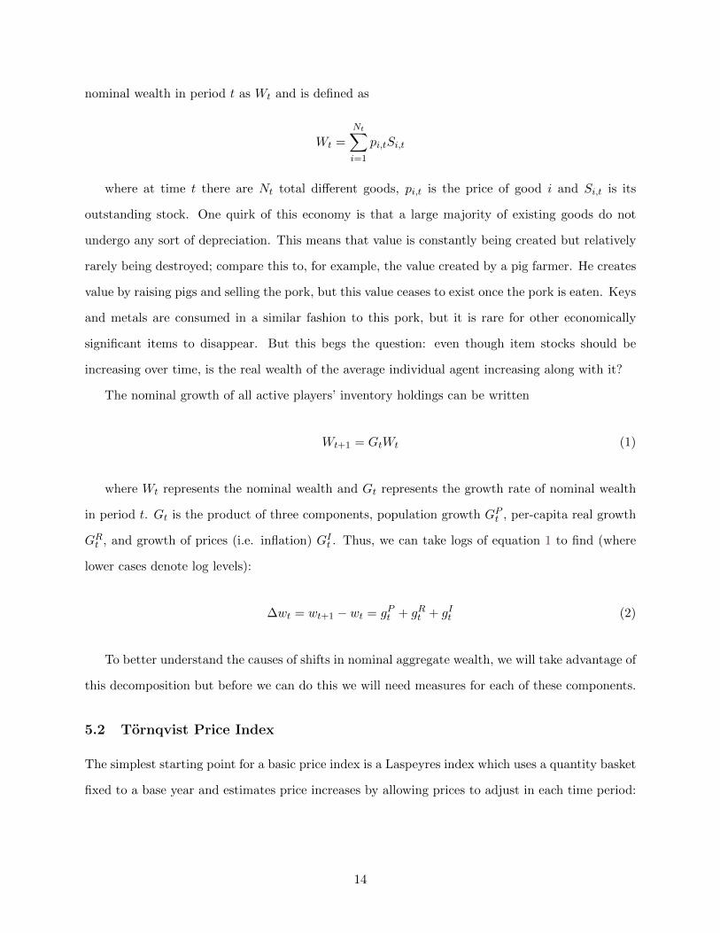
nominal wealth in period t as Wt and is defined as
Wt =
Nt∑i=1
pi,tSi,t
where at time t there are Nt total different goods, pi,t is the price of good i and Si,t is its
outstanding stock. One quirk of this economy is that a large majority of existing goods do not
undergo any sort of depreciation. This means that value is constantly being created but relatively
rarely being destroyed; compare this to, for example, the value created by a pig farmer. He creates
value by raising pigs and selling the pork, but this value ceases to exist once the pork is eaten. Keys
and metals are consumed in a similar fashion to this pork, but it is rare for other economically
significant items to disappear. But this begs the question: even though item stocks should be
increasing over time, is the real wealth of the average individual agent increasing along with it?
The nominal growth of all active players’ inventory holdings can be written
Wt+1 = GtWt (1)
where Wt represents the nominal wealth and Gt represents the growth rate of nominal wealth
in period t. Gt is the product of three components, population growth GPt , per-capita real growth
GRt , and growth of prices (i.e. inflation) GIt . Thus, we can take logs of equation 1 to find (where
lower cases denote log levels):
∆wt = wt+1 − wt = gPt + gRt + gIt (2)
To better understand the causes of shifts in nominal aggregate wealth, we will take advantage of
this decomposition but before we can do this we will need measures for each of these components.
5.2 Tornqvist Price Index
The simplest starting point for a basic price index is a Laspeyres index which uses a quantity basket
fixed to a base year and estimates price increases by allowing prices to adjust in each time period:
14

PLaspeyrest =
∑Ni pitqi0∑Ni pi0qi0
However, there is a particular problem with direct implementation of a basic Laspeyres index:
New items are constantly being introduced. If we choose a base period early in our timeline, we
will leave out all of the items which were introduced later on which are likely to be economically
important. But if we choose a base period late in our timeline, since there are some items which
did not exist earlier than the base, we can have no prices for items in early periods. And, indeed,
this is a significant issue for our environment. At the beginning of our data set, there are about
630 different item types traded, and at the end there are over 1600. The common alternative to a
basic Laspeyres index is a Paasche index. Paasche indices suffer from a closely related issue; they
take the quantity index from the current year in the denominator rather than quantities from the
base year. But we can have no prices in the base time period for items which were introduced
later on since we have no observed trades of goods that did not exist. Our strategy for solving this
problem is twofold. First, we use a modified Tornqvist index rather than Laspeyres or Paasche.
Second we use a hedonic model to estimate what prices for goods would have been just before their
introduction.
Our modified Tornqvist index (Tornqvist, 1936) modeled after the way the US C-CPI-U handles
its upper level price indices.4 The Tornqvist index is superlative and built from Translog preference
functions5. A Tornqvist price relative is as follows:
PTt,t−1 =
PtPt−1
=n∏i=1
(pi,tpi,t−1
) 12(pi,t−1qi,t−1
Vt−1+
pi,tqi,tVt
)
where Vt is the total nominal value of all goods in the quantity basket in period t, thuspi,tqi,tVt
is the expenditure share of good i in period t. The quantity index we use to calculate was built by
drawing a weekly sample of active players from the population and observing what those players
were holding in their backpack. For a detailed description of our sampling methodology, please see
Appendix B.
The Tornqvist index helps to avoid the problem discussed above with the simple Laspeyres:
4For more details, see Cage et al. (2003) and Bureau of Labor Statistics (2014) and ILO-IWGPS (2004).5See chapter 18 of the Export and Import Price Index Manual (2009) released by the IMF for a detailed discussion
of the advantages of superlative indices
15

−5.0
−2.5
0.0
2.5
5.0
Oct 2011 Jan 2012 Apr 2012 Jul 2012 Oct 2012 Jan 2013 Apr 2013Date
Log
Pric
ePrice Dynamics After Item Introductions
Figure 5: New item price time series.
Note: Each sparkline represents an item’s price over its first fifty days.
since the base period for each calculation is the previous period, the number of new items introduced
between base and current periods are minimized. As well, since the weights are value shares, new
items being introduced simply decreases the weights of already existing items so the index does not
increase due to increasing quantities of items. The chain Tornqvist price index from base period
t = 0 to period T is thus:
Chain PTT =
T∏t=1
(PTt,t−1
)One issue with our approach is due to the existence of items which are untradable - that is we
observe no prices – but which appear in our representative bundle. These items certainly have a
non-zero value and they do enter and leave people’s inventories, but we have no choice to exclude
these from our index. This is the same way that national statistical offices handle non-priced
services like family household services.
5.3 Hedonic Pricing Model
Another potential issue is that newly introduced items generally exhibit a commonality in price
trajectories, most new items start at a premium relative to similar items, and then steadily trade
16

lower in price. Figure 5 displays the price dynamics of items starting with their introduction and
tracing the time path of their log prices for the first fifty days thereafter. Log prices are used to
shrink the visual distance between item time series, hopefully helping to focus on general price
dynamics. Note that there are clusters of new items around Halloween and the December holidays.
Items with high starting prices (log price greater than 2.5, about 12 keys or more) appear to hold
their value in most cases, but items with lower initial values nearly always trend downward.
The Tornqvist price relative discussed above ignores items for which price information is not
present in adjacent periods, and thus the initial premium price on most new items is not captured
by the existing methodology. Though this issue is likely mitigated by the fact that new items are
infrequently traded and seen in relatively few inventories when first introduced–and so their weights
would be quite low–the omission of item introductions likely biases our price index downwards.
We deal with the problem of new item introductions by implementing a hedonic pricing model
(Diewert, 2003; Rosen, 1974) which estimates the prices of items based on that item’s characteristics
compared to the characteristics of other items with known prices. A similar hedonic price impu-
tation approach is used by national statistical bureaus to estimate prices in conditions of changes
in quality. We use the hedonic method as a best estimate of the initial values of each item based
on the item’s observable characteristics. This is accomplished by regressing dummies for each of
these characteristics interacted with time dummies on each item’s prices over time. For a given
time period, this gives an estimated value for each characteristic an item can have. If we apply the
assumption that an item’s value is approximated by the sum of values of its parts, we can estimate
the price of an arbitrary an item given only its vector of characteristics. We then use these imputed
prices as our best estimates for the value of items the day before they are introduced.
We impute unobserved prices via the following hedonic price model:
ln(pit) = α+ δtDt +
K∑k=1
(βkt · xik) + εit for t = 0, 1, ..., T (3)
For the price pit of item i in period t. Dt are fixed-effect time dummies (by week), xik is a
dummy indicating whether or not item i possesses item characteristic k (such characteristics are
time invariant), with error epsilon which has the standard assumption of being equal to zero in
expectation. Thus δt is the parameter on week t and βkt is the parameter on characteristic k in
17

week t.
The different characteristics xik we include in this model are item quality, class equipability as
some items can be used only by certain classes and others can be used by any class, item equip slot
such as weapon or hat, and finally a dummy indicating items held by a large proportion of active
players which took a value of 1 if 3% or more of users held the item and applied to less than 25%
of items. We believe that these characteristics sufficiently describe different items. We are limited
by the fact that a certain degree of the differentiation between items is due to non-quantifiable
aesthetics (e.g., two items can be identical with respect to the observables mentioned above, but
one of them might have art design that is in some sense “more attractive” and thus would command
a premium), but we believe that the number of different items is large enough that these will be
sufficiently averaged out when we conduct our regression.
6 Results
Our primary goal is the characterization of macroeconomic growth of this virtual barter environ-
ment. This requires the development of an aggregate price index and hedonic pricing models. Next,
we present possible explanations for some of the observed macro-level behavior. We conclude with
our analysis of the impact of micro-level shocks on individual items with evidence of an asset price
bubble, the first bubble to be documented in a barter market as far as we are aware.
6.1 Aggregate Price Level
In Figure 6, we present the calculated chain Tornqvist price index. Overall, the price level based
on representative backpack contents is relatively stable with slight deflation until approximately
mid-December of 2011, when there is a surge of inflation that is possibly related to a Christmas
event which brought an influx of new users into the game and introduced holiday-themed items
from new crates. This is followed by a dip towards the end of the first quarter of 2012 which proved
to be temporary as prices returns to their initial level and remain there for several months before
seeing steady inflation until October 2012, where we see the most striking feature of our price index.
Starting with the Halloween event of 2012, we see a sustained deflationary period. The overall price
level returns to its initial level around March 2012 and keeps falling until the end of our sample.
18

80
90
100
110
120
Jan 2012 Jul 2012 Jan 2013 Jul 2013Date
Pric
e In
dex
Chain Tornqvist Price Index, with Hedonic Imputed Prices (Base 2011−09−01)
Figure 6: Aggregate Price Index using Chain Tornqvist with Hedonically Imputed Prices
6.2 Hedonic Model
The hedonic hypothesis postulates that for any given period, a good is a bundling of potentially
time-varying price determining characteristics along with some possible aggregate price level effects
that change from period to period.6 Plotted in Figure 7 are the coefficients on the weekly fixed effect
dummies Dt along with their first and second standard errors bands. These can be interpreted as
an estimate for changes in the overall price level in a given week relative to the first week. Compare
Figure 6 to Figure 7; with the exception of a peak in the first quarter of 2012 which does not appear
in Figure 7, the dynamics are remarkably similar. These are both estimating the same thing using
entirely different methodology but both tell generally the same story.
Figure 8 plots how item characteristics have evolved over the sample using the hedonic model
from equation 3. In Figure 8 we see how quality premiums time series. For example, haunted
items tend to have their highest premiums around Halloween (technically, we observe haunted
items’ least discounts around Halloween – haunted items are essentially identical to unique items,
except for their text color and quality designation), but haunted quality items otherwise tend to
trade at a discount relative to unique items. Unusuals clearly trade at a consistent and increasing
premium relative to uniques and other qualities. Interestingly, in the weeks preceding Halloweens,
6Since item-level characteristics are fairly well defined in this context – item quality, character class equipablility,and broad item type – it may be informative to run a simplified hedonic regression which eliminates time-variationin the β coefficients. Results from such a model could be interpreted as the average value placed on each observablecharacteristic for items in our sample and are presented in Appendix C.
19

−0.4
−0.2
0.0
0.2
Oct 2011 Jan 2012 Apr 2012 Jul 2012 Oct 2012 Jan 2013 Apr 2013Date
Coe
ffici
ent
Week Dummy Coefficients (Relative to First Week)
Figure 7: Time dummy estimate from simple hedonic price model.
Note: Dark and light gray ribbons reflect first and second standard error bands respectively. Coefficient estimateson time dummies from model Equation 4.
unusuals exhibit an increase in their value premium. This is possibly due to the introduction of a
number of highly coveted Halloween themed visual effects (e.g. circling ghosts, cauldron bubbles,
and ‘’Demonflame”) at this time. Vintage items exhibit a consistently increasing premium relative
to uniques. Vintages are defined by their age, the plot may indicate a steadily increasing premium
as items age.
6.3 Aggregate Value and Growth
Figure 9 shows the total nominal value of all items in active players’ inventories (what we call
“market capitalization”) on a daily basis. This is calculated by taking the daily price of each item
multiplied by the outstanding quantity in active players’ inventories, and summed over all items.
We estimate that on the last day of our sample the total value of the economy was approximately
10 million keys – or using a very conservative US Dollar value exchange rate of $2 per key (keys are
available on the store at a price of $2.49, which acts as a price ceiling) – $20 million. Expanding
stocks to include all TF2 items from all users’ inventories, not just active players, market capital-
ization on the last day is over 50 million keys, or over $100 million. Note that towards the end
of our two year sample there appears to be a decline in aggregate value. This is explained by the
20

−2
0
2
4
Oct 2011 Jan 2012 Apr 2012 Jul 2012 Oct 2012 Jan 2013 Apr 2013Date
Coe
ffici
ent E
stim
ate,
with
One
Sta
ndar
d E
rror
Rib
bon
Quality Vintage Unusual Haunted Strange Genuine
Quality Coefficients Over Time
Figure 8: Coefficient estimates on time dummies interacted with item quality.
Note: Showing how premiums relative to unique have evolved over the trading sample. Standard error bands showsin transparent ribbons. Halloween 2011 and 2012 are indicated by vertical grey dashed lines.
0
5,000,000
10,000,000
15,000,000
Jan 2012 Jul 2012 Jan 2013 Jul 2013Date
Key
s
Nominal Aggregate Value of Active TF2 Player Inventories
Figure 9: Nominal aggregate value of active TF2 player inventories.
Note: Keys are sold on the store for $2.49 each
21

0%
50%
100%
150%
Oct 2011 Jan 2012 Apr 2012 Jul 2012 Oct 2012 Jan 2013 Apr 2013Date
Prices Per−Capita Real Wealth Population
Nominal Growth
Figure 10: Growth of nominal active player wealth
Note: Nominal growth since August 2011. Aggregate nominal value of active player wealth is the product of prices,population, and per-capita real inventory values. The natural log of nominal wealth is thus plotted as the stack ofthese logged components.
decline in price level causing the bulk of commonly-held items (usually traded for metals) to drop
in value with respect to our numeraire.
In previous sections, we elucidated the trends of the price level and per-capita real wealth.
Applying those to this decomposition along with data regarding changes in active population results
in Figure 10. The levels displayed are all in percentage terms with respect to the levels in period
0. E.g. at the beginning of July 2012, the nominal economy is approximately 120% larger than it
was at the beginning, of which approximately 10% can be attributed to growth in the price level,
35% of which can be attributed to growth in real per-capita wealth, and the remainder attributed
to growth in the number of active players.
We see that real per-capita inventories generally displayed a slowly increasing contribution to
the total growth for the duration of our sample. It also shows that practically all of the volatility
displayed in Figure 9 can be explained by volatility in the population of active players and that
there is actually a steady and increasing contribution to economic growth from the real per-capita
component. This signifies a healthy and growing economy, even during periods which players are
22

rapidly switching between being active and inactive.
Prices consistently increase after January 2012 until a peak in October 2012, thereafter steadily
pulling down net growth until the end of the sample. It can be seen that the contribution from
prices disappears (and in fact becomes negative) on precisely the date just after January 2013 at
which the price index in Figure 6 shows that the price level dips below its starting point of 100.
6.4 Nominal Rigidities and the Decline of the Price Level
Here, we present a plausible case in which this decreasing value of metals can translate to a decreas-
ing aggregate price level. We observe that items tend to be primarily traded for a single currency.
Low value items tend to trade for metals, mid value items tend to trade for keys, high value items
tend to trade for Bill’s Hats, and very high value items tend to trade for Earbuds as a result of the
indivisibility of these currencies. It is therefore difficult to profit from currency arbitrage across
“value-tiers” of items. It is this combination of price rigidities across currency denominations along
with depreciation of metals that may have led to the sustained deflation we observe.
Our best explanation for the deflation towards the end of the sample is monetary and due to
the quirks of a barter system with multiple de facto commodity currency goods. See Figure 11 for
the daily spot exchange rates between keys and each alternative currency. Notice that decline in
the price level starts at the end of 2013 – as seen in the price index in Figure 6 – syncing up with
a sustained appreciation of keys against metals in Figure 11. This appreciation is quite significant:
at the beginning of our sample it took a little more than two refined metals to purchase a key,
but towards the end it took nearly six metals. Thus, the metal-price of keys more than doubled
over this period. Also interesting to note is that the path of Bill’s Hats/Key and Earbuds/Key
exchange rates track each other closely (with a few exceptions near the end of the sample). This
may imply that the higher-value currency goods are better substitutes for each other than the
low-value metals, and is also likely due to the fixed nature of supply of these good items compared
to the increasing supply of metals and keys. A more complete analysis of this potential source of
depreciation is presented in Appendix D.
To illustrate this point, consider how profitable arbitrage would occur if one currency (metal)
is becoming devalued relative to the other currencies but metal prices remained fixed. One would
trade metals for goods, then trade those goods for non-metal currencies, then trade the non-metal
23

0.0
0.2
0.4
0.6
Jan 2012 Jul 2012 Jan 2013 Jul 2013Date
Exc
hang
e R
ate
Key Per Refined Metal Exchange Rate
0
5
10
Jan 2012 Jul 2012 Jan 2013 Jul 2013Date
Exc
hang
e R
ate
Keys Per Bill's Hat Exchange Rate
0
10
20
30
Jan 2012 Jul 2012 Jan 2013 Jul 2013Date
Exc
hang
e R
ate
Keys Per Earbud Exchange Rate
Figure 11: Inter-money exchange rates
Note: Daily median exchange rate with three-week smoothing. Grey ribbons reflect first and third quartiles ofobserved daily exchanges, meaning 50% of trades occurred within gray ribbon. 31 Oct 2012 indicated by a blackdotted line in the top figure. 24

currencies back for more metal than they started with. This is only worth it if costs associated
with trading the goods for non-metal currency is lower than the surplus from completing the cycle.
If these search and transactions costs too high enough, it is not worth it to engage in the
arbitrage that would keep prices constant across all currencies. We see that as metal-key exchange
rates decline and the value of metal to decreases, this does not appear to fully translate to the
metal-price of metal-denominated items. Indeed, we see that for most metal-denominated items,
their key-prices fall at precisely the same rate as the rate of depreciation of metal. Thus, as the
key-price of metals drops, the key-prices of metal-denominated items tend to drop with it. This
leads to the component of our quantity bundle which consists of items that are primarily traded
for metals to drop in lock-step with the metal depreciation. If this component of the aggregate
quantity index is “large”, it alone can drive large movements in our aggregate prices.
We argue that this is due to frictions imposed by a barter market. If buyers were equally
willing to pay with keys as metals for the purchase any good, it is likely that the prices of goods
as denominated in the more consistently valued currency would be constant and there would be an
increase in the price in terms of the currency which sees a declining value. But, if most traders will
only offer metals for some subset of goods because it is impractical to trade for goods which are
worth a tenth of a key or less using keys or higher value currencies, such a scenario is plausible.
We now present evidence for the presence of nominal rigidities discussed above, which would
imply that items which happen to be priced in terms of metals – likely due to their low value and
therefore difficulty in trading with indivisible higher value commodity currencies – have their value
linked to the value of metals.
We investigate this by linking the frequency that metal is used to pay for items to the price
change from Oct 2012 to the May 2013. We estimate the following weighted OLS model:
ρi = β0 + β1 ·mi + εi
In this regression, mi represents the value proportion of SM trades for item i in which the item
trades for metal and thus 1−mi is the value proportion of trades which the item was exchanged for
non-metal currencies. For example, an item that always traded for metals would have an mi of 1
and an item for which half of the value of trades was from metals and half was from keys, mi would
25

be .5. The regression relies on value share percentages derived from October 2012 observations
and these value share percentages hold a 0.95 correlation with observations in May 2013, implying
that these value shares seem relatively stable over our time horizon. The dependent variable ρi
represents the percent change of the price of item i with respect to this item’s price in October 12,
2012, just before the start of the deflationary period.
The model is weighted by the total value of each item i in the month of October 2012, thus
more economically significant items were given heavier weights. We only looked at items for which
prices were observed in both Oct 2012 and May 2013, there were 1,288 such items. We remove
observations for which percent price changes were above the 99th or below the 1st percentile, leaving
1256 items with prices in both periods.
The interpretation of this regression is straight forward: the sign of the coefficient on mi tells
us if items which were primarily traded for metals tended to undergo price increases (positive β1)
or price decreases (negative β1) over the period of deflation which started in October 2012.
Table 2: Regression Estimates from WOLS of Price Change on the Trading Value Share of Metal.
Dependent variable:
Percent Change in Price
Metal Value Share −0.1867∗∗∗ (0.0406)Constant −26.0422∗∗∗ (1.4763)
Observations 1,256R2 0.0166
Note: ∗p<0.1; ∗∗p<0.05; ∗∗∗p<0.01
Our regression coefficients are reported in Table 2. It shows that a one-percent increase in the
value of metal an item tends to trade in Oct. 2012 is correlated with an additional 0.18% drop
in price between Oct 2012 and May 2013. Thus overall on average, items that traded 100% with
metals tended to experience an 18% decrease in price compared to items which never traded for
metals. This is evidence that items which trade primarily for metals tend to have a corresponding
decline in price. But the decline in price is also less than the decline in the exchange rate of metals
(approximately 50% from October 2012 to May 2013, as can be seen in Figure 11) which means
that this is likely only a part of the whole story.
26

0.00
0.25
0.50
0.75
Jul−2011 Jan−2012 Jul−2012 Jan−2013Date
Pric
e in
Syn
thet
ic K
eys
Fancy Fedora Price Time Series
0
50000
100000
150000
Jul−2011 Jan−2012 Jul−2012 Jan−2013Date
Sto
cks
Stocks of Fancy Fedora Over all TF2 Players
Figure 12: Price time series of the unique (normal) quality Fancy Fedora.
Notes: The date of the store retirement announcement is indicated by a dashed red line, and the actual retirementdate is indicated by the second dotted line, in blue.
6.5 Response of Individual Items to Micro-level Shocks
We conclude our results with a discussion of the impact on individual items of micro-level shocks.
Notice in Figure 12, the price of the Fancy Fedora starts high and over a few months drops down
and stabilizes, as is typical for newly introduced items.7 But at the beginning of 2013, there is
a sudden spike in interest. This is driven by a 10 Jan 2013 announcement, as indicated by a red
dashed line, that this hat and 8 others would be “retired” on 25 Jan 2013 as indicated by a blue
dotted line. Retirement of these items means that they are no longer acquirable except by trading
with other players and thus the total supply would be capped at the current level on 25 Jan.
This announcement led to rampant speculation on these items which drove up the price by
approximately 120% over the two week time period between announcement and retirement. But
this price boost ultimately proved to be temporary as the price falls almost as rapidly as it surged
in the first place. This represents the first evidence of a possible speculative bubble in a barter
market that we are aware of.
7The price time series was generated using trailing price estimates rather than the centered prices discussedabove. This was because centered prices cause price estimates to increase before the announcement which is notrepresentative of what was happening in the market on this day.
27

Figure 12 also shows the stocks of Fancy Fedoras. On January 10, 2013 there were 178,400,
which increased by 2.26% to 182,440 by January 25th. Our best explanation is that there was
a sufficient quantity of these hats in existence to satisfy the demand for them for the purpose of
durable consumption at the price of approximately 0.2 keys, but the retirement announcement
caused a positive demand shock as market participants anticipated a negative future supply shock,
driving up current prices (red dashed line). Soon after this negative supply shock took place (blue
dotted line), it became clear that the act of fixing supply did not actually do much to shrink quantity
available and – as well as the fact that there are likely a large number of close substitutes and the
influx of supply by speculators after the January 10 announcement – meant that people interested
in durable consumption of the item could simply buy a different hat that didn’t see the price more
than double. Thus, the announcement and subsequent retirement did not effectively change long
run demand and had a small but positive effect on long run supply, so the price returned to its
initial level and the speculators that went long on them figuratively lost their shirts.
Another item example demonstrating clear market responses to micro-shocks is the strange
Scattergun, a strange-quality version of the default class weapon of the Scout. Strange quality
items are notable because they record some sort of player statistic while the player uses the item
(e.g. a counter that tracks total number of other players killed with the gun).
On 9 October, as shown in Figure 13 with a red dotted line, these stranges were suddenly made
available from a newly introduced and particularly ubiquitous series of locked crates and found
inside these crates with a probability of approximately 20%. The effect of this policy shock on
supply can be seen in Figure 13. The total stock on October 9, 2012 was approximate 71,000 and
had been increasing at the rate of approximately 50 per day for months. After this new crate was
introduced the rate of increase of the inventory stock suddenly exploded, after one month there
were more than 101,000 strange Scatterguns in existence. After three months, these stocks had
doubled.
The impact of this sudden large positive supply shock can clearly be seen in the price of the gun,
depicted in Figure 13. In contrast to the story of the Fancy Fedora, in which the retirement of an
item did not appear to have a long lasting impact on the market supply or demand leading to long
run prices being the same as before the retirement, this event obviously actually impacts the long-
run supply which causes an unambiguous decrease in long-run market price. Thus, individual prices
28

0
1
2
Jul−2011 Jan−2012 Jul−2012 Jan−2013 Jul−2013Date
Pric
e in
Syn
thet
ic K
eys
Strange Scattergun Price Time Series
0
50000
100000
150000
200000
Jul−2011 Jan−2012 Jul−2012 Jan−2013 Jul−2013Date
Sto
cks
Stocks of Strange Scattergun Over all TF2 Players
Figure 13: Price time series of the strange quality Scattergun.
Note: The red dotted line is at October 9th, the date which the item became more widely available.
in the economy do indeed appear to respond to specific micro-level shocks in the ways consistent
with basic microeconomic intuition given the direction of the shocks to supply and demand.
7 Conclusion
With this work, we present an examination of an economy which is interesting for at least two
reasons. First, it is a remarkably rich dataset which documents a true barter market, the likes of
which have been pondered by economists for centuries. Second, it’s a virtual economy consisting
entirely of non-tangible goods which people nonetheless assign value to.
Our primary goal was to calculate macroeconomic growth in this novel environment and con-
cluded that an increasing component of nominal growth was due to increases in real per-capita
holdings. Per-capita real wealth displays a slow and steady growth for the duration of our sample
and most of the volatility in aggregate economic value can be explained by volatility in the active
player population.
We presented a hedonic pricing model which we used to impute prices for a Tornqvist price
index. We show that not all classes are created equal when it comes to item values. The index
29

indicates that the price level tended to rise until October of 2012, at which point the price level
starts declining due at least in part to the declining value of metals. We then traced the source
of this depreciation of metals to a shock to both the stocks of metals and keys as well as the rate
of increase of their respective supplies.8 We then demonstrated that items which trade for metals
tended to have prices that decreased as the value of metals declined, indicating possible nominal
rigidities. But the price decline was less than the decline of the value of metals, so this is likely not
the only thing affecting these items. Thus we did find evidence that macro-indicators responded to
macro-level shocks.
Finally, we find in these virtual economies evidence of the same sorts of forces which evidently
influence “real world” markets in our micro-level case studies. If a credible central authority makes
some decree that could increase expectations of future prices, prices move in that direction. If there
is a sudden exogenous positive supply shock in the market for a specific good, the price of that good
falls. These goods are but two of many items that have been impacted by idiosyncratic shocks, and
their behavior is mirrored in similar goods which were subjected to similar shocks. None of this
news should be surprising, but it supports our position that other such virtual economies (which
are certainly only going to become more common in the coming years) are fertile ground for further
research and the fact that these virtual economies will typically have impeccable record keeping
should be enough to get researchers excited.
Future work will investigate the emergence and evolution of number of fundamental market
institutions in the tradition of Radford (1945), Burdett et al. (2001), and Lankenau (2001) and
we will search for the origin of media of exchange and the development of trade intermediaries
by mapping trade networks and behaviors of these intermediaries. In doing so, we hope to answer
questions related to how much surplus such intermediary activity brings to the economy as a whole,
and how is that surplus is distributed amongst various types of users, deep questions that go to the
heart of classic economic inquiry9 and are issues which many modern economists have struggled to
answer empirically.
8See Appendix D9See Smith (1776), Jevons (1885), and Menger (1892)
30

References
George A Akerlof. The market for “lemons”: Quality uncertainty and the market mechanism. The
Quarterly Journal of Economics, pages 488–500, 1970.
Kenneth Burdett, Alberto Trejos, and Randall Wright. Cigarette money. Journal of Economic
Theory, 99.1:117–142, 2001.
United States Bureau of Labor Statistics. BLS handbook of methods. US Department of Labor,
Bureau of Labor Statistics, 2014.
Robert Cage, John Greenlees, and Patrick Jackman. Introducing the chained consumer price index.
In International Working Group on Price Indices (Ottawa Group): Proceedings of the Seventh
Meeting, pages 213–246. Paris: INSEE, 2003.
Edward Castronova. A test of the law of demand in a virtual world: Exploring the petri dish
approach to social science. Technical report, CESifo working paper, 2008.
Edward Castronova, Dmitri Williams, Cuihua Shen, Rabindra Ratan, Li Xiong, Yun Huang, and
Brian Keegan. As real as real? macroeconomic behavior in a large-scale virtual world. New
Media & Society, 11(5):685–707, 2009.
W Erwin Diewert. Hedonic regressions: a review of some unresolved issues. In 7th Meeting of the
Ottawa Group, Paris, May, pages 27–29, 2003.
International Monetary Fund. Export and import price index manual: theory and practice. IN-
TERNATIONAL MONETARY FUND, 2009.
ILO-IWGPS. Consumer price index manual: Theory and practice. 2004.
William Stanley Jevons. Money and the Mechanism of Exchange, volume 17. 1885.
Stephen E Lankenau. Smoke’em if you got’em: Cigarette black markets in us prisons and jails.
The Prison Journal, 81(2):142–161, 2001.
Karl Menger. On the origin of money. The Economic Journal, 2(6):239–255, 1892.
Robert A Radford. The economic organisation of a pow camp. Economica, pages 189–201, 1945.
31
Sherwin Rosen. Hedonic prices and implicit markets: product differentiation in pure competition.
The Journal of Political Economy, pages 34–55, 1974.
Adam Smith. An inquiry into the nature and causes of the wealth of nations: Volume one. 1776.
Leo Tornqvist. The bank of finlands consumption price index. Bank of Finland Monthly Bulletin,
10(1936):1–8, 1936.
32

Appendix
A Price Weighting Methodology
We use a number of different approaches in generating weights to assign to individual observations
in estimating daily prices. Broadly, these approaches fit into two categories: “Centered” and
“Trailing” (or Leading).
A.1 Centered Prices Weighted Mean
To calculate an item’s mean price for a specific day, we start with an interval of seven days. We
collect all SM price observations from three days previous to three days into the future and remove
any price observations above the 9th decile and below the 1st decile. We drop these extremes
because almost all items have many price observations which are clear outliers and means are
sensitive to such outliers. We then apply a triangular (or, more precisely a trapezoidal) weighting
function as illustrated in Figure 14
There are initially three days on either side of the day which we are estimating prices for. Many
items are very high volume and thus we have lots of price observations but for some items, there is
relatively low enough volume such that even including a full week does not give us a large enough
number of observations that we are confident in their prices.
Start of Day
24 Hour Interval
Total Time Interval(starts at 7 days)
Total weight sums to one
Time
Figure 14: Weighting function
To account for this issue, we define a control system which utilizes the coefficient of variation:
33

cv = σµ , where µ and σ are the mean and standard deviation of our sample. Our control system sets
a cutoff value for coefficient of variation c∗v and we calculate the coefficient for each item in a given
time period citv and if i is true that citv > c∗v, we increase the window for that item on that day by one
day and recalculate. This process is repeated until the window includes sufficient observations such
that citv ≤ c∗v. The cutoff we use for this process is c∗v = .5 a this number appears to consistently
select an appropriate window width.
B Representative Basket Derivation Methodology
In consumer inflation indexes like CPI these quantities strive to reflect typical consumption baskets.
In contrast, quantities reflect producer purchases in input producer price indexes and in the Gross
Domestic Product deflator they reflect production quantities. Our quantity index reflects the bundle
of goods held by a “representative player.”
B.1 Methodology
These representative player inventories were generated by drawing random samples of users from
the active player population, where an active player is defined as one who logged into Team Fortress
2 within ninety days of the sample date. We identify the average quantity of each TF2 item held in
the sampled inventories. But there are some unique issues with our sampling in this environment
due to the presence of an upper tail of inventory value distributions composed of people with very
large inventory values. These HNWIs are rare enough that we almost certainly will not have a good
balance of them represented in each time period’s active player sample. Increasing our sample size
sufficiently beyond 1% of the population is also technically infeasible given the number of active
players (typically more than 250,000 each week) many of whom possess scores of items. Without
adjustment, the price index could exhibit big movements from one period to the next due more to
sudden shifts in the quantity index than shifts in price.
Our approach to dealing with these HNWIs is first to tag the top proportion of wealth-holding
individual users as HNWIs, where we define the inventory value cutoff as a nominal inventory value
above 800 keys, or approximately $1600. If an active player is classified as a HNWI in one of these
censuses, their inventories are logged each week for the entire year and they are excluded from the
34

non-HNWI sample for that year. These HNWI players account for approximately 0.3 to 0.4 percent
of the active player population.
We then track inventories of all HNWIs each period along with the random 1% sample of non-
HNWIs, and derive average item inventories for each group. The composition of the basket derived
from these 1% samples does not fluctuate greatly from time period to time period. Finally, the
HNWI and non-HNWI representative inventories are combined weighting item quantities based on
each groups’ relative proportion of the overall active player population at each period.10
All inventory data excludes individuals who have marked their “Steam Profile” as private. Of
the approximately 1,500 unique active players classified as HNWIs, 255 have been excluded due to
this privacy restriction on their their backpacks. Our methodology thus assumes the omission of
these privacy preferring players does not significantly bias the representativeness of our HNWI and
non-HNWI sample.
Once representative baskets are found for each tier, they are average together weighted by the
relative proportion of each group to the overall population.
C Hedonic Estimates of Values of Item Characteristics
Equation 4 presents the hedonic model we estimate. We use this simplified version because the
model with time dummies has thousands of regression coefficients, far too many to report in a
single table. The full model from Equation 3, however, was used to produce Figures 7 and 8:
ln (pit) = αt +K∑k=1
(βk · xit) + εit for t = 0, ..., T (4)
For item i in period t, price pit is a function of weekly time dummies, K time-invariant item
characteristics, and an error process. Table 3 shows the coefficient estimates of the hedonic regres-
sion.
All TF2 items are associated with a single “quality”. We used the unique quality for our
regression as it is by far the most common as the baseline, and estimates for each item are premiums
or discounts relative to that item’s unique version. These results suggest that vintage items have
tended to trade a full 180% above more normal unique quality ones. All unique quality items that
10Our representative basket derivation methodology is discussed in more detail in Appendix B
35

Table 3: Hedonic Price Model with Time Unvarying Characteristic Dummies
Dependent variable:
log price
Quality (mutually exclusive), Relative to Unique Quality
Genuine 0.9035∗∗∗ (0.0054)
Haunted −0.9255∗∗∗ (0.0077)
Other 5.5827∗∗∗ (0.0621)
Strange 1.9038∗∗∗ (0.0051)
Unusual 3.7819∗∗∗ (0.0042)
Vintage 1.0300∗∗∗ (0.0045)
Item Type (mutually exclusive) Relative to Action Items
Cosmetic 0.4629∗∗∗ (0.0098)
Tool −0.0655∗∗∗ (0.0111)
Weapon −0.5792∗∗∗ (0.0105)
Character Class Equippablility (non-exclusive)
Spy Equippable 0.2507∗∗∗ (0.0041)
Engineer Equippable −0.0392∗∗∗ (0.0042)
Soldier Equippable 0.1775∗∗∗ (0.0037)
Sniper Equippable 0.0674∗∗∗ (0.0043)
Demoman Equippable −0.0869∗∗∗ (0.0039)
Medic Equippable 0.0983∗∗∗ (0.0043)
Pyro Equippable 0.0663∗∗∗ (0.0038)
Heavy Equippable −0.0318∗∗∗ (0.0039)
Scout Equippable 0.2527∗∗∗ (0.0039)
Widely Held Item −1.5229∗∗∗ (0.0033)
(>3% of Active Players)
With Week Time Dummies X
Observations 734,066
R2 0.7449
Adjusted R2 0.7449
Residual Std. Error 1.093(df = 733853)
F Statistic 1.88e+04∗∗∗ (df = 114; 733853 )
Note: Standard errors in parentheses, and ∗p<0.1; ∗∗p<0.05; ∗∗∗p<0.01
36

existed on or before September 20th 2010, when TF2 trading was introduced, were redesignated as
vintage. Unusual quality items tend to attract the highest premium, a full 43000% premium above
uniques. All unusual quality items possess some kind of visual effect, like flames, orbiting planets,
or stinky-smelly lines. Unusual items are particularly rare, as they only appear with a very small
probability from opening a crate and cannot come from any other source, and it is this rarity which is
likely the reason which they command prices much higher than those of non-unusual items. Strange
items, which will track in-game statistics, tend to exhibit a 571% premium above uniques. Quality
“other” appears to attract the highest premium, however, items of this quality only appeared due
to extremely unusual circumstances, akin to very rare coins minted with imperfections which make
them very valuable to dedicated coin collectors but unavailable and inconsequential to everyone
else, and accounting for only a negligible fraction of all coins. And, like coins, it is likely that some
owners of the oddities are not even aware of the item’s value. Thus we tend to see an extremely
small number of transactions involving items of quality “other”, but those transactions indicate
that they are worth a small fortune. These, however, are not very representative of the broader
economy.
All tools, weapons, and cosmetic items may be used by only one, some, or all character classes.
Unlike quality or item type, this is non-exclusive designation. Character classes vary in speed,
strength, and other abilities. For example medics are able heal teammates, and heavies are slow
but may inflict and withstand a lot of damage. The highest equipability premiums come from items
that can be carried by scouts and spies. Should an item be equipable by a scout, for example, it
will tend to garner a 29% premium relative to a similar item that is not equipable by the scout.
Items that are held by a relatively large percentage of active players, defined as items that
appear in more than 3% of active player inventories, tend to exhibit a large discount, trading for
78% lower than items that are not so widely held. To ensure this characteristic is time unvarying,
the percentage holding statistic is taken on average over the whole sample. This is included in the
regression to account for the potential price implication of an item’s relative scarcity.
37

1,500,000
2,000,000
2,500,000
Oct 2012 Jan 2013 Apr 2013 Jul 2013 Oct 2013 Jan 2014Date
Sto
cks
InterventionPeriod Pre Update Post Update
Figure 15: Regression discontinuity on Refined Metal stocks
400,000
500,000
600,000
700,000
800,000
900,000
Oct 2012 Jan 2013 Apr 2013 Jul 2013 Oct 2013 Jan 2014Date
Sto
cks
InterventionPeriod Pre Update Post Update
Figure 16: Regression discontinuity on Key stocks
38

D Decline of the Aggregate Price Level
Figure 15 shows the outstanding item stocks of the primary currency metal, refined metals. Notice
that right at the end of October, 2012, there is a sudden increase in the rate at which refined metals
are entering into the economy. We argue that this is due to a major content update released on 26
October 2012. This date marks the point in time at which metals started their precipitous drop in
value. This apparent positive supply shock appears to have been temporary, as the rate that metal
stocks increase swiftly returns to a rate of increase only marginally higher than its rate prior to the
event. But the fact that the rate of change of the stock of metals slowed did not correspond to a
slowing rate of depreciation.
Figure 16 sheds some light on this question. Simultaneous with the sudden burst of metals
that entered the economy, there was a sudden negative supply shock to our numeraire, keys. This
corresponds to the major content update including new types of crates, leading to many more keys
being consumed than purchased for a short period. The supply of metals suddenly increased and
the supply of keys suddenly decreased; naturally, we would expect this to lead to an increase in the
number of metals required to receive a key in exchange. The rate of increase of keys also appears to
slow somewhat. This trend is confirmed by a regression discontinuity analysis using the following
regression equation:
Stocki = β0 + β1DaysToPatchi + β2PostPatchi + β3Interactioni + εi
Where DaysToPatch is the number of days until the update went live, PostPatch is a dummy
variable that takes a value of zero on days which were prior to October 26 and a value of one after,
and Interaction is the product of these two variables. Our regression estimates are presented in
Table 4. β1 can be interpreted as the pre-update rate of expansion of the money supply for each
currency and β1 +β3 is the post-update rate of expansion of that currency, thus β3 is the difference
in the trends before and after the cutoff.
Table 4 shows that the daily rate of increase in the stock of keys dropped from 1,810 to ap-
proximately 1,065, a 41% reduction. Simultaneously, the rate of change of metals increases slightly
from 2,560 to 2,689, an 5% increase. This could explain the sudden and continuous depreciation;
39

Table 4: Before and After Halloween Time Trends for Keys (1) and Metals (2)
Dependent variable:
Item Stocks
(1) (2)
DaysToPatch 1,810∗∗∗ 2,560∗∗∗
(59) (47)
PostPatch −90,924∗∗∗ 78,012∗∗∗
(4,552) (3,649)
Interaction −745∗∗∗ 129∗∗∗
(60) (48)
Constant 572,952∗∗∗ 1,457,520∗∗∗
(3,976) (3,187)
Observations 500 500R2 0.977 0.998
Note: ∗p<0.1; ∗∗p<0.05; ∗∗∗p<0.01
before October 26, keys were entering the economy at a rate that was not too far off of the rate that
refined metals were entering, but after this event the rates at which the goods entered the economy
differed drastically, leading to relative supplies drifting further and further away from each other.
The depreciation of metals can clearly be seen when comparing the nominal and real values of
our representative basket. These are presented in Figures ?? and ??, respectively. The real value in-
creases at an approximately constant rate as the average holdings of a representative agent increases
over time, but the nominal value levels off and starts to decline right as the metal depreciation starts.
This is due to the fact that the most commonly held items are generally metal-denominated and
these items see shrinking key-values starting in October of 2012.
40