SOEPpaperson Multidisciplinary Panel Data Research

Aggregation and Labor Supply Elasticities

Alois Kneip, Monika Merz, Lidia Storjohann

606 201

3SOEP — The German Socio-Economic Panel Study at DIW Berlin 606-2013

SOEPpapers on Multidisciplinary Panel Data Research at DIW Berlin This series presents research findings based either directly on data from the German Socio-Economic Panel Study (SOEP) or using SOEP data as part of an internationally comparable data set (e.g. CNEF, ECHP, LIS, LWS, CHER/PACO). SOEP is a truly multidisciplinary household panel study covering a wide range of social and behavioral sciences: economics, sociology, psychology, survey methodology, econometrics and applied statistics, educational science, political science, public health, behavioral genetics, demography, geography, and sport science. The decision to publish a submission in SOEPpapers is made by a board of editors chosen by the DIW Berlin to represent the wide range of disciplines covered by SOEP. There is no external referee process and papers are either accepted or rejected without revision. Papers appear in this series as works in progress and may also appear elsewhere. They often represent preliminary studies and are circulated to encourage discussion. Citation of such a paper should account for its provisional character. A revised version may be requested from the author directly. Any opinions expressed in this series are those of the author(s) and not those of DIW Berlin. Research disseminated by DIW Berlin may include views on public policy issues, but the institute itself takes no institutional policy positions. The SOEPpapers are available at http://www.diw.de/soeppapers Editors: Jürgen Schupp (Sociology) Gert G. Wagner (Social Sciences, Vice Dean DIW Graduate Center) Conchita D’Ambrosio (Public Economics) Denis Gerstorf (Psychology, DIW Research Director) Elke Holst (Gender Studies, DIW Research Director) Frauke Kreuter (Survey Methodology, DIW Research Professor) Martin Kroh (Political Science and Survey Methodology) Frieder R. Lang (Psychology, DIW Research Professor) Henning Lohmann (Sociology, DIW Research Professor) Jörg-Peter Schräpler (Survey Methodology, DIW Research Professor) Thomas Siedler (Empirical Economics) C. Katharina Spieß (Empirical Economics and Educational Science)

ISSN: 1864-6689 (online)

German Socio-Economic Panel Study (SOEP) DIW Berlin Mohrenstrasse 58 10117 Berlin, Germany Contact: Uta Rahmann | soeppapers@diw.de

Aggregation and Labor Supply Elasticities

Alois Kneip University of Bonn

Monika Merz University of Vienna, CEPR and IZA

Lidia Storjohann University of Bonn

ABSTRACT

The aggregate Frisch elasticity of labor supply has played a key role in business cycle analysis. This paper develops a statistical aggregation procedure which allows for worker heterogeneity in observables and unobservables and is applicable to an individual labor supply function with non-employment as a possible outcome. Performing a thought experiment in which all offered or paid wages are subject to an unanticipated temporary change, we can derive an analytical expression for the aggregate Frisch elasticity and illustrate its main components: (i) the intensive and extensive adjustment of hours worked, (ii) the extensive adjustment of wages, and (iii) the aggregate employment rate. We use individual-specific data from the German Socio-Economic Panel (SOEP) for males at working-age in order to quantify each component. This data base provides indirect evidence on non-employed workers’ reservation wages. We use this variable in conjunction with a twostep conditional density estimator to retrieve the extensive adjustment of hours worked and wages paid. The intensive hours’ adjustment follows from estimating a conventional panel data model of individual hours worked. Our estimated aggregate Frisch elasticity varies between .63 and .70. These results are sensitive to the assumed nature of wage changes.

JEL Classification: C51, E10, J22

Keywords: aggregation, reservation wage distribution, labor supply, extensive and intensive margin of adjustment, time-varying Frisch elasticities

Corresponding author: Monika Merz Department of Economics University of Vienna Oskar-Morgenstern-Platz 1 1090 Vienna Austria E-mail: monika.merz@univie.ac.at

1 Introduction

The aggregate Frisch elasticity of labor supply has been at center stage in modern business

cycle analysis for many years. It was first introduced into the literature by Ragnar Frisch

and continues to be of interest from a theoretical as well as from an empirical perspective.

At any point in time, it measures the reaction of total hours worked to a small change in

the mean wage when wealth is held constant. The exact size of this particular elasticity

matters a lot when macroeconomists try to assess the quantitative implications of certain

types of policies on employment and hours worked. For example, changes in monetary

or fiscal policy parameters which directly or indirectly impact a worker’s net wage rate

typically lead to a change in total labor supply. In spite of its relevance, the size of

this aggregate change cannot easily be determined when worker heterogeneity is taken

seriously. That is because the reaction of total labor supply is a highly complex object

whose various components need to be accounted for. This object not only depends on

the distribution of wage rates across employed workers and that of reservation wage rates

across non-employed workers. It also depends on the hours’ adjustment of existing workers

(intensive margin) as well as of those who move between employment and non-employment

following a wage change (extensive margin). Lastly, the overall reaction depends on the

exact implementation of the underlying policy change.

In this paper, we develop a unified framework which allows us to simultaneously study

the role that workers’ participation and hours decisions play for the size of the aggregate

Frisch elasticity. We depart from MaCurdy’s (1985) standard intertemporal labor supply

model that features complete markets, uncertainty and worker heterogeneity in observable

and unobservable characteristics. We then modify the statistical aggregation approach

developed by Paluch, Kneip and Hildenbrand (2012) to allow for a corner solution in

a worker’s labor supply decision. This procedure has the distinct advantage of being

widely applicable, because it requires neither a particular preference structure nor specific

distributional assumptions for explanatory variables. We use it to aggregate our individual

labor supply functions and wage rates. In order to derive the aggregate Frisch elasticity of

labor supply, we subject all offered or paid wages to an unanticipated temporary increase.

By eliminating wealth effects and taking account of the implied adjustment of labor supply,

we derive an analytical expression for the aggregate elasticity and illustrate its components:

(i) the intensive and extensive adjustment of hours worked, (ii) the extensive adjustment

of wages, and (iii) the aggregate employment rate.

To empirically implement our aggregation approach, we rely on specific econometric

models and estimate them using micro-level data from the German Socio-Economic Panel

(SOEP). The SOEP is unique in that it provides evidence on non-employed workers’

reservation wage rates. This variable is essential for estimating the adjustment of hours

worked and wages paid of workers who change their participation decision – so-called

movers. We estimate the adjustment of hours worked along the intensive margin, i.e., of

stayers, with the help of a standard panel model. Our sample comprises German males

1

who are between 25 and 64 years old and live in former West Germany, because their labor

supply behavior is well captured by the intertemporal model. Our estimation results yield

an average individual Frisch wage-elasticity of .29 – a value that stands in sharp contrast

to our estimated aggregate values which vary between .63 and .70 over the period ranging

from 2000 to 2008.

We are not the first ones to study the aggregate Frisch elasticity of labor supply in an

environment with heterogeneous workers. Our work is related to two main strands of the

literature. First, it relates to the many contributions in modern business cycle analysis

where the aggregate Frisch elasticity enters as key entity that affects the reaction of total

labor supply to a change in wages induced by policy or exogenous disturbances. The basic

idea goes back to Lucas and Rapping (1969) which is considered as the origin of intertem-

poral labor supply in modern macroeconomics. Employment lotteries as introduced into

the literature by Hansen (1985) and Rogerson (1988) have illustrated the importance of

the extensive margin adjustment for the aggregate Frisch wage-elasticity, but except for

the ex post status of a worker in the labor force it ignores worker heterogeneity. More

closely related to our work are the papers by Chang and Kim (2005; 2006) who allow for

worker heterogeneity and explore how the size of the aggregate Frisch elasticity of hours

worked varies with incomplete markets. They focus on the intensive margin only. The

work by Gourio and Noual (2009) is also relatively closely related to ours. They use a

complete market setup to explore the role of ‘marginal workers’ who by definition are

indifferent between working and not working for adjustment along the extensive margin

when wages change. All these contributions commonly use a parameterized version of

a structural utility function which makes it possible to derive a functional relationship

between the aggregate labor supply and aggregate wages. They differ with respect to

the type and degree of worker heterogeneity, the assumed market structure, and whether

they focus on the intensive or the extensive margin of adjusting labor supply. Another

related piece is by Fiorito and Zanella (2012). They use the PSID to empirically explore

the link between the micro and the macro Frisch wage-elasticity without deriving an exact

analytical relationship between them. They nicely illustrate how the difference between

the individual and the aggregate Frisch elasticity changes for various subpopulations, but

they cannot measure the extensive margin. Second, our work relates to the growing micro

literature that has produced estimates of the individual wealth-compensated wage elas-

ticity of hours worked since the early work by MaCurdy (1981; 1985) and Altonji (1986).

Their estimates for males range from .10 to .45, and from 0 to .35, respectively. The

recent study by Chetty et al. (2012) provides quasi-experimental evidence on individual

wage-elasticities. Its conclusion that the intensive margin of .5 is twice as large as the

extensive one is juxtaposed to a central finding of the labor supply literature summarized

in Blundell and MaCurdy (1999) that the extensive margin matters most for explaining

variation in total person hours over the business cycle.

Our contribution to this literature is twofold. First, we develop a statistical aggre-

gation approach which does not require specific assumptions about model parameters or

2

distributions of explanatory variables. It is comprehensive enough to simultaneously cap-

ture adjustment along the intensive and the extensive margin when wage rates change

unexpectedly in an environment where workers are heterogeneous. Secondly, we illustrate

the importance of statistical aggregation by empirically implementing it using the Ger-

man SOEP which contains as special feature information on reservation wage rates for

non-employed workers.

This paper is organized as follows. Section 2 presents a dynamic model of individual

labor supply under uncertainty. Section 3 develops a general statistical aggregation proce-

dure that features labor supply adjustment along the intensive and the extensive margin

and is used to derive an analytical expression for the aggregate Frisch wage-elasticity of

labor supply. Section 4 specifies the two econometric models used for empirical estimation,

a panel data model on hours worked and a two-stage procedure to estimate conditional

densities. Section 5 presents our database and introduces the main variables used for

estimation. Section 6 reports all estimation results. Section 7 concludes.

2 A Dynamic Labor Supply Model

Underlying our aggregation exercise is an individual-specific labor supply function which

relates the amount of labor that an individual supplies to the market in any given period

t to a set of determinants. We view this function as the outcome of an intertemporal

optimization problem under uncertainty.1 In what follows we sketch this problem including

the preferences, the constraints and the informational setting for each individual. For the

sake of notational simplicity, we abstain from introducing a person-specific index until

section 4.

Consider an infinitely-lived consumer. Her preferences are captured by a momentary

utility function U which depends on private consumption c, leisure l, a vector of observable

individual characteristics X and a vector of unobservable individual variables Z, including

tastes and talents. U is assumed to be twice differentiable, separable over time and also

in consumption c and market hours worked h. Furthermore, U is strictly increasing and

concave in c and h. When choosing sequences of leisure, consumption and future asset

holdings to maximize her expected life-time utility, the consumer takes the real wage rate w

and the real market return on assets r as given and respects the following two constraints:

First, the per-period time-constraint

Tt ≥ lt + ht (1)

which equates the available time T to the sum of leisure and market hours worked h in

each period. Second, the budget constraint

ct + at+1 ≤ wtht + (1 + rt)at (2)

1Our model exposition closely follows that in MaCurdy (1985).

3

that sets the sum of consumption expenditures and the change in asset holdings at+1− atequal to total earnings plus interest income from current period asset holdings at. A

consumer starts life with initial assets a0.

Denoting by Et the mathematical expectation conditional on information known at the

beginning of time t and by 0 < β < 1 the discount rate, the consumer’s choice problem

can be summarized as follows:

max{ct,lt,at+1}∞t=0

E0

∞∑t=0

βtU(ct, lt;Xt, Zt) (3)

subject to equations (1), (2), the non-negativity constraints ct > 0, lt ≥ 0, and the

initial condition a0 > 0.2 For any differentiable function f(x1, . . . , xn) let ∂xif(x1, . . . , xn)

denote the partial derivative with respect to the i-th component. Then, letting λt denote

the Lagrange multiplier associated with the period t budget constraint, the first-order

necessary conditions for utility maximization are given by:

∂cU(·)− λt = 0 (4a)

∂lU(·)− λtwt = 0 (4b)

λt = βEt[(1 + rt+1)λt+1]. (4c)

With the help of the implicit function theorem equations (4a) and (4b) can be solved for

individual consumption and labor supply as functions of the form

ct = d(wt, λt, Xt, Zt) (5)

ht = g(wt, λt, Xt, Zt). (6)

The time-invariant functions d(·) and g(·) depend only on the specifics of the utility func-

tion U(·) and on whether corner solutions are optimal for hours worked in period t. These

functions contain two types of arguments, namely those that capture what is going on

in the current period – wt, Xt and Zt – and λt which is a sufficient statistic for past

and future information relevant for the individual’s current choices. If we further assume

consumption and leisure to be normal goods, the concavity of the utility function implies

∂λd < 0, ∂wg ≥ 0, ∂λg ≥ 0. (7)

Equation (4c) summarizes the stochastic process governing λt. Assuming interest rates

do not vary stochastically, this process can alternatively be expressed as an expectational

difference equation:

λt = β(1 + rt+1)Etλt+1.

2A complete formulation of the consumer’s dynamic decision problem also requires a transversalitycondition for wealth: lim

T→∞λT aT = 0.

4

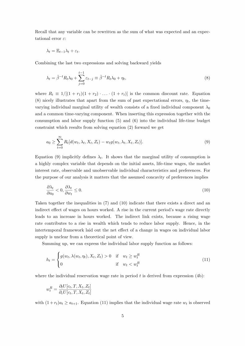
Recall that any variable can be rewritten as the sum of what was expected and an expec-

tational error ε:

λt = Et−1λt + εt.

Combining the last two expressions and solving backward yields

λt = β−tRtλ0 +t−1∑j=0

εt−j ≡ β−tRtλ0 + ηt, (8)

where Rt ≡ 1/[(1 + r1)(1 + r2) · . . . · (1 + rt)] is the common discount rate. Equation

(8) nicely illustrates that apart from the sum of past expectational errors, ηt, the time-

varying individual marginal utility of wealth consists of a fixed individual component λ0

and a common time-varying component. When inserting this expression together with the

consumption and labor supply function (5) and (6) into the individual life-time budget

constraint which results from solving equation (2) forward we get

a0 ≥∞∑t=0

Rt[d(wt, λt, Xt, Zt)− wtg(wt, λt, Xt, Zt)]. (9)

Equation (9) implicitly defines λt. It shows that the marginal utility of consumption is

a highly complex variable that depends on the initial assets, life-time wages, the market

interest rate, observable and unobservable individual characteristics and preferences. For

the purpose of our analysis it matters that the assumed concavity of preferences implies

∂λt∂a0

< 0,∂λt∂wt

≤ 0. (10)

Taken together the inequalities in (7) and (10) indicate that there exists a direct and an

indirect effect of wages on hours worked. A rise in the current period’s wage rate directly

leads to an increase in hours worked. The indirect link exists, because a rising wage

rate contributes to a rise in wealth which tends to reduce labor supply. Hence, in the

intertemporal framework laid out the net effect of a change in wages on individual labor

supply is unclear from a theoretical point of view.

Summing up, we can express the individual labor supply function as follows:

ht =

g(wt, λ(wt, ηt), Xt, Zt) > 0 if wt ≥ wRt0 if wt < wRt

(11)

where the individual reservation wage rate in period t is derived from expression (4b):

wRt =∂lU [ct, T,Xt, Zt]

∂cU [ct, T,Xt, Zt]

with (1 + rt)at ≥ at+1. Equation (11) implies that the individual wage rate wt is observed

5

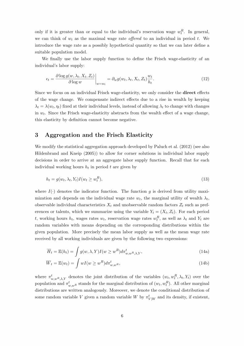
only if it is greater than or equal to the individual’s reservation wage wRt . In general,

we can think of wt as the maximal wage rate offered to an individual in period t. We

introduce the wage rate as a possibly hypothetical quantity so that we can later define a

suitable population model.

We finally use the labor supply function to define the Frisch wage-elasticity of an

individual’s labor supply:

εt =∂ log g(w, λt, Xt, Zt)

∂ logw

∣∣∣∣w=wt

= ∂wg(wt, λt, Xt, Zt)wtht. (12)

Since we focus on an individual Frisch wage-elasticity, we only consider the direct effects

of the wage change. We compensate indirect effects due to a rise in wealth by keeping

λt = λ(wt, ηt) fixed at their individual levels, instead of allowing λt to change with changes

in wt. Since the Frisch wage-elasticity abstracts from the wealth effect of a wage change,

this elasticity by definition cannot become negative.

3 Aggregation and the Frisch Elasticity

We modify the statistical aggregation approach developed by Paluch et al. (2012) (see also

Hildenbrand and Kneip (2005)) to allow for corner solutions in individual labor supply

decisions in order to arrive at an aggregate labor supply function. Recall that for each

individual working hours ht in period t are given by

ht = g(wt, λt, Yt)I(wt ≥ wRt ), (13)

where I(·) denotes the indicator function. The function g is derived from utility maxi-

mization and depends on the individual wage rate wt, the marginal utility of wealth λt,

observable individual characteristics Xt and unobservable random factors Zt such as pref-

erences or talents, which we summarize using the variable Yt = (Xt, Zt). For each period

t, working hours ht, wages rates wt, reservation wage rates wRt , as well as λt and Yt are

random variables with means depending on the corresponding distributions within the

given population. More precisely the mean labor supply as well as the mean wage rate

received by all working individuals are given by the following two expressions:

Ht = E(ht) =

∫g(w, λ, Y )I(w ≥ wR)dπtw,wR,λ,Y , (14a)

W t = E(wt) =

∫wI(w ≥ wR)dπtw,wR , (14b)

where πtw,wR,λ,Y

denotes the joint distribution of the variables (wt, wRt , λt, Yt) over the

population and πtw,wR

stands for the marginal distribution of (wt, wRt ). All other marginal

distributions are written analogously. Moreover, we denote the conditional distribution of

some random variable V given a random variable W by πtV |W and its density, if existent,

6

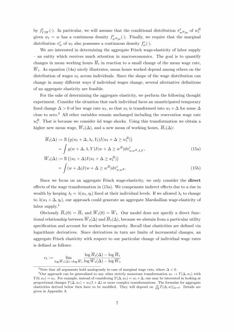
by f tV |W (·). In particular, we will assume that the conditional distribution πtwR|w of wRt

given wt = w has a continuous density f twR|w(·). Finally, we require that the marginal

distribution πtw of wt also possesses a continuous density f tw(·).We are interested in determining the aggregate Frisch wage-elasticity of labor supply

– an entity which receives much attention in macroeconomics. The goal is to quantify

changes in mean working hours Ht in reaction to a small change of the mean wage rate,

W t. As equation (14a) nicely illustrates, mean hours worked depend among others on the

distribution of wages wt across individuals. Since the shape of the wage distribution can

change in many different ways if individual wages change, several alternative definitions

of an aggregate elasticity are feasible.

For the sake of determining the aggregate elasticity, we perform the following thought

experiment. Consider the situation that each individual faces an unanticipated temporary

fixed change ∆ > 0 of her wage rate wt, so that wt is transformed into wt + ∆ for some ∆

close to zero.3 All other variables remain unchanged including the reservation wage rate

wRt . That is because we consider iid wage shocks. Using this transformation we obtain a

higher new mean wage, W t(∆), and a new mean of working hours, Ht(∆):

Ht(∆) := E(g(wt + ∆, λt, Yt)I(wt + ∆ ≥ wRt )

)=

∫g(w + ∆, λ, Y )I(w + ∆ ≥ wR)dπtw,wR,λ,Y , (15a)

W t(∆) := E((wt + ∆)I(wt + ∆ ≥ wRt )

)=

∫(w + ∆)I(w + ∆ ≥ wR)dπtw,wR . (15b)

Since we focus on an aggregate Frisch wage-elasticity, we only consider the direct

effects of the wage transformation in (15a). We compensate indirect effects due to a rise in

wealth by keeping λt = λ(wt, ηt) fixed at their individual levels. If we allowed λt to change

to λ(wt + ∆, ηt), our approach could generate an aggregate Marshallian wage-elasticity of

labor supply.4

Obviously Ht(0) = Ht and W t(0) = W t. Our model does not specify a direct func-

tional relationship between W t(∆) and Ht(∆), because we abstain from a particular utility

specification and account for worker heterogeneity. Recall that elasticities are defined via

logarithmic derivatives. Since derivatives in turn are limits of incremental changes, an

aggregate Frisch elasticity with respect to our particular change of individual wage rates

is defined as follows:

et := limlogW t(∆)→logW t

logHt(∆)− logHt

logW t(∆)− logW t

3Note that all arguments hold analogously in case of marginal wage cuts, where ∆ < 0.4Our approach can be generalized to any other strictly monotone transformation wt → T (∆, wt) with

T (0, wt) = wt. For example, instead of considering T (∆, wt) = wt+∆, one may be interested in looking atproportional changes T (∆, wt) = wt(1 + ∆) or more complex transformations. The formulae for aggregateelasticities derived below then have to be modified. They will depend on ∂

∂∆T (∆, w)|∆=0. Details are

given in Appendix A.

7

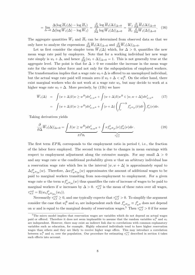
= lim∆→0

∆(logHt(∆)− logHt)

∆(logW t(∆)− logW t)=

∂∂∆ logHt(∆)|∆=0

∂∂∆ logW t(∆)|∆=0

=W t

Ht

∂∂∆Ht(∆)|∆=0

∂∂∆W t(∆)|∆=0

. (16)

The aggregate quantities W t and Ht can be determined from observed data so that we

only have to analyze the expressions ∂∂∆Ht(∆)|∆=0 and ∂

∂∆W t(∆)|∆=0.

Let us first consider the simpler term W t(∆) which, for ∆ > 0, quantifies the new

mean wage rate paid by employers. Note that for a working individual her new wage

rate simply is wt + ∆, and hence ∂∂∆(wt + ∆)|∆=0 = 1. This is not generally true at the

aggregate level. The point is that for ∆ > 0 we consider the increase in the mean wage

rate for the entire labor force and not only for the subpopulation of employed workers.

The transformation implies that a wage rate wt+∆ is offered to an unemployed individual,

but the actual wage rate paid will remain zero if wt + ∆ < wRt . On the other hand, there

exist marginal workers who do not work at a wage rate wt, but may decide to work at a

higher wage rate wt + ∆. More precisely, by (15b) we have

W t(∆) =

∫(w + ∆)I(w ≥ wR)dπtw,wR +

∫(w + ∆)I(wR ∈ [w,w + ∆])dπtw,wR (17)

=

∫(w + ∆)I(w ≥ wR)dπtw,wR +

∫(ν + ∆)

(∫ ν+∆

ν

f twR|ν(ν)dν

)f tw(ν)dν.

Taking derivatives yields

∂

∂∆W t(∆)|∆=0 =

∫I(w ≥ wR)dπtw,wR︸ ︷︷ ︸

EPRt

+

∫νf twR|ν(ν)f tw(ν)dν︸ ︷︷ ︸

τextw,t

. (18)

The first term EPRt corresponds to the employment ratio in period t, i.e., the fraction

of the labor force employed. The second term is due to changes in mean earnings with

respect to employment adjustment along the extensive margin. For any small ∆ > 0

and any wage rate w the conditional probability given w that an arbitrary individual has

a reservation wage rate which lies in the interval [w,w + ∆] is approximately equal to

∆f twR|w(w). Therefore, ∆wf t

wR|w(w) approximates the amount of additional wages to be

paid to marginal workers transiting from non-employment to employment. For a given

wage rate w the term wf twR|w(w) thus quantifies the rate of increase of wages to be paid to

marginal workers if w increases by ∆ > 0. τ extw,t is the mean of these rates over all wages,

τ extw,t = E(wtftwR|wt(wt)).

Necessarily τ extw,t ≥ 0, and one typically expects that τ extw,t > 0. To simplify the argument

consider the case that wRt and wt are independent such that f twR|w ≡ f

twR

does not depend

on w and is equal to the marginal density of reservation wages.5 Then τ extw,t > 0 if for some

5The micro model implies that reservation wages are variables which do not depend on actual wagespaid or offered. Therefore it does not seem implausible to assume that the random variables wRt and wtare independent. However, there may exist an indirect link due to correlations with common explanatoryvariables such as education, for example. Highly educated individuals tend to have higher reservationwages than others and they are likely to receive higher wage offers. This may introduce a correlationbetween wRt and wt over the population. Our procedure for estimating τextw,t described in section 4 takessuch effects into account.

8

wage rate ν with f tw(ν) > 0 we also have f twR

(ν) > 0. In other words, τ extw,t > 0 if there

exists some overlap between the support of the distributions of wages wt and the support

of the distribution of reservation wages wRt . This will typically be fulfilled for any real

economy.

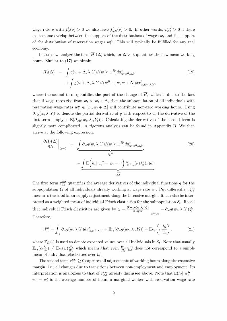
Let us now analyze the term Ht(∆) which, for ∆ > 0, quantifies the new mean working

hours. Similar to (17) we obtain

Ht(∆) =

∫g(w + ∆, λ, Y )I(w ≥ wR)dπtw,wR,λ,Y (19)

+

∫g(w + ∆, λ, Y )I(wR ∈ [w,w + ∆])dπtw,wR,λ,Y ,

where the second term quantifies the part of the change of Ht which is due to the fact

that if wage rates rise from wt to wt + ∆, then the subpopulation of all individuals with

reservation wage rates wRt ∈ [wt, wt + ∆] will contribute non-zero working hours. Using

∂wg(w, λ, Y ) to denote the partial derivative of g with respect to w, the derivative of the

first term simply is E(∂wg(wt, λt, Yt)). Calculating the derivative of the second term is

slightly more complicated. A rigorous analysis can be found in Appendix B. We then

arrive at the following expression:

∂Ht(∆)

∂∆

∣∣∣∣∆=0

=

∫∂wg(w, λ, Y )I(w ≥ wR)dπtw,wR,λ,Y︸ ︷︷ ︸

τ inth,t

(20)

+

∫E(ht| wRt = wt = ν

)f twR|ν(ν)f tw(ν)dν︸ ︷︷ ︸

τexth,t

.

The first term τ inth,t quantifies the average derivatives of the individual functions g for the

subpopulation Et of all individuals already working at wage rate wt. Put differently, τ inth,t

measures the total labor supply adjustment along the intensive margin. It can also be inter-

preted as a weighted mean of individual Frisch elasticities for the subpopulation Et. Recall

that individual Frisch elasticities are given by εt = ∂ log g(w,λt,Yt)∂ logw

∣∣∣∣w=wt

= ∂wg(wt, λ, Y )wtht .

Therefore,

τ inth,t =

∫Et∂wg(w, λ, Y )dπtw,wR,λ,Y = EEt(∂wg(wt, λt, Yt)) = EEt

(εthtwt

), (21)

where EEt(·) is used to denote expected values over all individuals in Et. Note that usually

EEt(εt htwt ) 6= EEt(εt)Ht

W twhich means that even W t

Htτ inth,t does not correspond to a simple

mean of individual elasticities over Et.The second term τ exth,t ≥ 0 captures all adjustments of working hours along the extensive

margin, i.e., all changes due to transitions between non-employment and employment. Its

interpretation is analogous to that of τ extw,t already discussed above. Note that E(ht| wRt =

wt = w) is the average number of hours a marginal worker with reservation wage rate

9

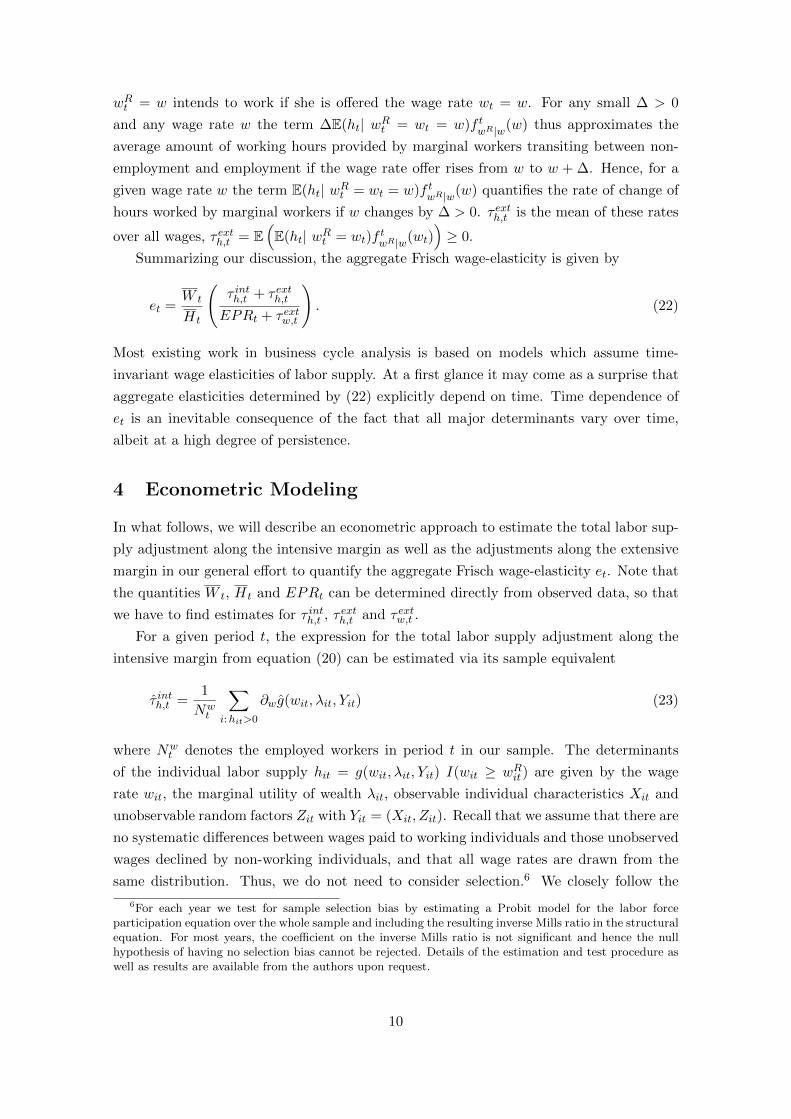
wRt = w intends to work if she is offered the wage rate wt = w. For any small ∆ > 0

and any wage rate w the term ∆E(ht| wRt = wt = w)f twR|w(w) thus approximates the

average amount of working hours provided by marginal workers transiting between non-

employment and employment if the wage rate offer rises from w to w + ∆. Hence, for a

given wage rate w the term E(ht| wRt = wt = w)f twR|w(w) quantifies the rate of change of

hours worked by marginal workers if w changes by ∆ > 0. τ exth,t is the mean of these rates

over all wages, τ exth,t = E(E(ht| wRt = wt)f

twR|w(wt)

)≥ 0.

Summarizing our discussion, the aggregate Frisch wage-elasticity is given by

et =W t

Ht

(τ inth,t + τ exth,t

EPRt + τ extw,t

). (22)

Most existing work in business cycle analysis is based on models which assume time-

invariant wage elasticities of labor supply. At a first glance it may come as a surprise that

aggregate elasticities determined by (22) explicitly depend on time. Time dependence of

et is an inevitable consequence of the fact that all major determinants vary over time,

albeit at a high degree of persistence.

4 Econometric Modeling

In what follows, we will describe an econometric approach to estimate the total labor sup-

ply adjustment along the intensive margin as well as the adjustments along the extensive

margin in our general effort to quantify the aggregate Frisch wage-elasticity et. Note that

the quantities W t, Ht and EPRt can be determined directly from observed data, so that

we have to find estimates for τ inth,t , τ exth,t and τ extw,t .

For a given period t, the expression for the total labor supply adjustment along the

intensive margin from equation (20) can be estimated via its sample equivalent

τ inth,t =1

Nwt

∑i:hit>0

∂wg(wit, λit, Yit) (23)

where Nwt denotes the employed workers in period t in our sample. The determinants

of the individual labor supply hit = g(wit, λit, Yit) I(wit ≥ wRit ) are given by the wage

rate wit, the marginal utility of wealth λit, observable individual characteristics Xit and

unobservable random factors Zit with Yit = (Xit, Zit). Recall that we assume that there are

no systematic differences between wages paid to working individuals and those unobserved

wages declined by non-working individuals, and that all wage rates are drawn from the

same distribution. Thus, we do not need to consider selection.6 We closely follow the

6For each year we test for sample selection bias by estimating a Probit model for the labor forceparticipation equation over the whole sample and including the resulting inverse Mills ratio in the structuralequation. For most years, the coefficient on the inverse Mills ratio is not significant and hence the nullhypothesis of having no selection bias cannot be rejected. Details of the estimation and test procedure aswell as results are available from the authors upon request.

10

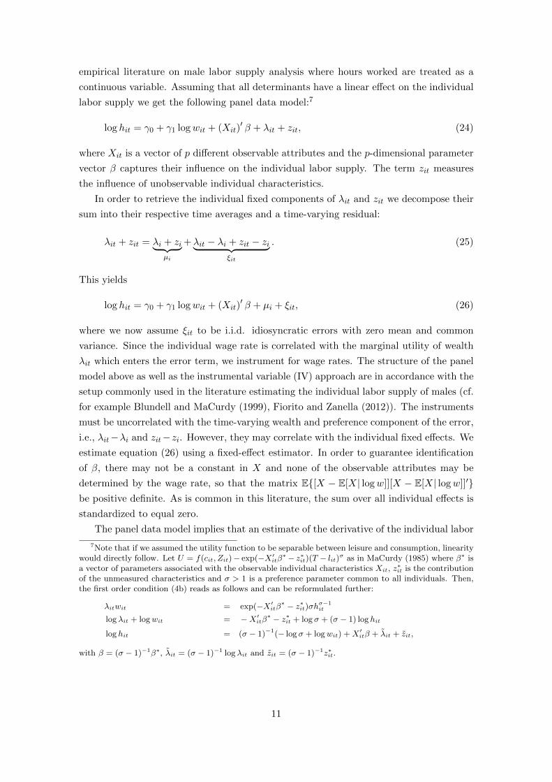
empirical literature on male labor supply analysis where hours worked are treated as a

continuous variable. Assuming that all determinants have a linear effect on the individual

labor supply we get the following panel data model:7

log hit = γ0 + γ1 logwit + (Xit)′ β + λit + zit, (24)

where Xit is a vector of p different observable attributes and the p-dimensional parameter

vector β captures their influence on the individual labor supply. The term zit measures

the influence of unobservable individual characteristics.

In order to retrieve the individual fixed components of λit and zit we decompose their

sum into their respective time averages and a time-varying residual:

λit + zit = λi + zi︸ ︷︷ ︸µi

+λit − λi + zit − zi︸ ︷︷ ︸ξit

. (25)

This yields

log hit = γ0 + γ1 logwit + (Xit)′ β + µi + ξit, (26)

where we now assume ξit to be i.i.d. idiosyncratic errors with zero mean and common

variance. Since the individual wage rate is correlated with the marginal utility of wealth

λit which enters the error term, we instrument for wage rates. The structure of the panel

model above as well as the instrumental variable (IV) approach are in accordance with the

setup commonly used in the literature estimating the individual labor supply of males (cf.

for example Blundell and MaCurdy (1999), Fiorito and Zanella (2012)). The instruments

must be uncorrelated with the time-varying wealth and preference component of the error,

i.e., λit−λi and zit−zi. However, they may correlate with the individual fixed effects. We

estimate equation (26) using a fixed-effect estimator. In order to guarantee identification

of β, there may not be a constant in X and none of the observable attributes may be

determined by the wage rate, so that the matrix E{[X − E[X| logw]][X − E[X| logw]]′}be positive definite. As is common in this literature, the sum over all individual effects is

standardized to equal zero.

The panel data model implies that an estimate of the derivative of the individual labor

7Note that if we assumed the utility function to be separable between leisure and consumption, linearitywould directly follow. Let U = f(cit, Zit)− exp(−X ′itβ∗− z∗it)(T − lit)σ as in MaCurdy (1985) where β∗ isa vector of parameters associated with the observable individual characteristics Xit, z

∗it is the contribution

of the unmeasured characteristics and σ > 1 is a preference parameter common to all individuals. Then,the first order condition (4b) reads as follows and can be reformulated further:

λitwit = exp(−X ′itβ∗ − z∗it)σhσ−1it

log λit + logwit = −X ′itβ∗ − z∗it + log σ + (σ − 1) log hit

log hit = (σ − 1)−1(− log σ + logwit) +X ′itβ + λit + zit,

with β = (σ − 1)−1β∗, λit = (σ − 1)−1 log λit and zit = (σ − 1)−1z∗it.

11

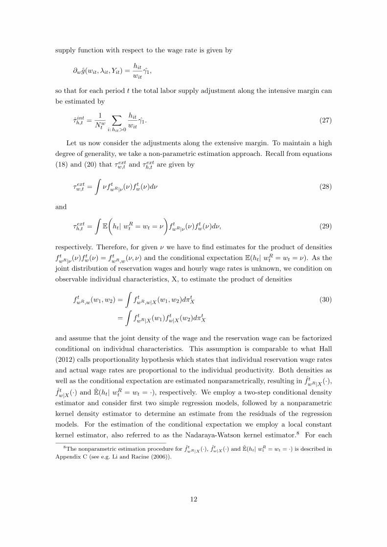
supply function with respect to the wage rate is given by

∂wg(wit, λit, Yit) =hitwit

γ1,

so that for each period t the total labor supply adjustment along the intensive margin can

be estimated by

τ inth,t =1

Nwt

∑i:hit>0

hitwit

γ1. (27)

Let us now consider the adjustments along the extensive margin. To maintain a high

degree of generality, we take a non-parametric estimation approach. Recall from equations

(18) and (20) that τ extw,t and τ exth,t are given by

τ extw,t =

∫νf twR|ν(ν)f tw(ν)dν (28)

and

τ exth,t =

∫E(ht| wRt = wt = ν

)f twR|ν(ν)f tw(ν)dν, (29)

respectively. Therefore, for given ν we have to find estimates for the product of densities

f twR|ν(ν)f tw(ν) = f t

wR,w(ν, ν) and the conditional expectation E(ht| wRt = wt = ν). As the

joint distribution of reservation wages and hourly wage rates is unknown, we condition on

observable individual characteristics, X, to estimate the product of densities

f twR,w(w1, w2) =

∫f twR,w|X(w1, w2)dπtX (30)

=

∫f twR|X(w1)f tw|X(w2)dπtX

and assume that the joint density of the wage and the reservation wage can be factorized

conditional on individual characteristics. This assumption is comparable to what Hall

(2012) calls proportionality hypothesis which states that individual reservation wage rates

and actual wage rates are proportional to the individual productivity. Both densities as

well as the conditional expectation are estimated nonparametrically, resulting in f twR|X(·),

f tw|X(·) and E(ht| wRt = wt = ·), respectively. We employ a two-step conditional density

estimator and consider first two simple regression models, followed by a nonparametric

kernel density estimator to determine an estimate from the residuals of the regression

models. For the estimation of the conditional expectation we employ a local constant

kernel estimator, also referred to as the Nadaraya-Watson kernel estimator.8 For each

8The nonparametric estimation procedure for f twR|X(·), f tw|X(·) and E(ht| wRt = wt = ·) is described in

Appendix C (see e.g. Li and Racine (2006)).

12

period t, τ extw,t and τ exth,t can then be approximated by

τ extw,t =

∫ν

(1

Nt

∑i

f twR|X=Xit(ν)f tw|X=Xit

(ν)

)dν (31)

and

τ exth,t =

∫E(ht| wRt = wt = ν

)( 1

Nt

∑i

f twR|X=Xit(ν)f tw|X=Xit

(ν)

)dν (32)

where Nt denotes the sum of working and non-working individuals in period t in our

sample. This allows us to estimate the aggregate Frisch wage-elasticity as specified in

equation (22) for any period t.

5 Data

Our empirical work is based on data from the German Socio-Economic Panel (SOEP), a

representative sample of private households and individuals living in Germany. The panel

was started in 1984 (wave A) and has been updated annually through 2011 (wave BB).

The panel design closely follows that of the Panel Study of Income Dynamics (PSID) –

a representative sample of US households and individuals – but also takes idiosyncrasies

of the German legal and socio-economic framework into account.9 Since 2000, the SOEP

covers on average 12,000 households and 20,000 individuals per year. A set of core ques-

tions is asked every year, including questions on education and training, labor market

behavior, earnings, taxes and social security, etc.

We use the SOEP, because we consider it particularly well suited for the purpose of

our analysis. To our knowledge it is the only micro panel currently available that contains

indirect information on reservation wage rates of non-employed workers. This variable is

essential for our effort to quantify changes in a worker’s participation decision. Apart from

detailed information on individual characteristics, the SOEP also reports an employed

individual’s market hours worked and earnings. We can thus compute an individual’s

hourly wage rate.

5.1 Sample

For the sake of our empirical analysis we need consistent data on individual labor market

behavior over a rather long time horizon. Therefore, we focus on the working age popula-

tion of German males living in former West Germany who are between 25 and 64 years old.

We do so, because we are neither interested in the peculiarities of women’s working behav-

ior nor in the institutional differences between former East and West Germany. Including

females in a relatively long panel study would be problematic because in Germany, unlike

9A detailed description of the panel’s design, its coverage, the main questions asked, etc. is containedin the Desktop Companion to the SOEP, which is accessible online at www.diw.de.

13

in many other countries, females have undergone severe changes in their labor market

behavior during the past decades and are less attached to the workforce than elsewhere.

Since we want to focus on those who actively participate in the labor market, we exclude

retirees, individuals in military service under conscription or in community service which

can serve as substitute for compulsory military service, and individuals currently under-

going education. We also exclude individuals with missing information on unemployment

experience or the amount of education or training. A maximum of 56 individuals is af-

fected. Our sample ranges from 2000 to 2009. That is because in 2000 a refreshment

sample was added to the SOEP which effectively doubled the number of observations.

Moreover, our fixed-effect estimation procedure requires the time index t to converge to

infinity to ensure consistent estimates of the individual fixed effects. Therefore, we create a

balanced panel from our sample which includes those working males who are continuously

employed over the sample period. Our balanced panel comprises 1,296 individuals. We

use these individuals whenever we compute measures related to employed workers. For all

questions related to non-employment we consider individuals who are not employed and

have answered the question on reservation wages. This leaves us with 91 to 140 individuals

between 2000 and 2009.10

5.2 Variables

Our key variables of interest are the hourly wage rate and actual working hours for the

employed, the reservation wage rate for the unemployed, and individual characteristics.11

A person’s total hours worked, hit, are given by the average actual weekly working hours.

There is a wide range of answers to the question “And how much on average does your

actual working week amount to, with possible overtime?” – answers range from 5.5 to

80 hours per week. In fact, the distribution of hit is not discrete in nature, but quite

dispersed, in particular during the last 15 to 20 years. It seems that the traditional 40

hours workweek gradually loses its prevalence as there are increasing possibilities of part-

time work, higher skilled workers are asked to work more, and more flexible work options

have become available.12

The hourly wage rate is calculated by dividing the current net monthly earnings by

the product of 4.3 and contractual weekly working hours. We use net earnings, since

information on the reservation wage is only available in net terms and we need the wage

rate, wit, and the reservation wage rate to be comparable. We convert all nominal values

into real ones by dividing all nominal expressions by the consumer price index which uses

2005 as base year.

The reservation wage is generated from answers to the question “How much would the

net pay have to be for you to consider taking the job?” which is posed to all individuals

10A detailed description of our sample is given in Appendix D. In particular, Table 6 shows summarystatistics and we list all refinements to the original data.

11A list of all SOEP variables with respective names as well as a list of all generated variables withdescription is given in Appendix D.

12Histograms of actual hours worked for the years 2000, 2005 and 2009 are available in Appendix D.

14

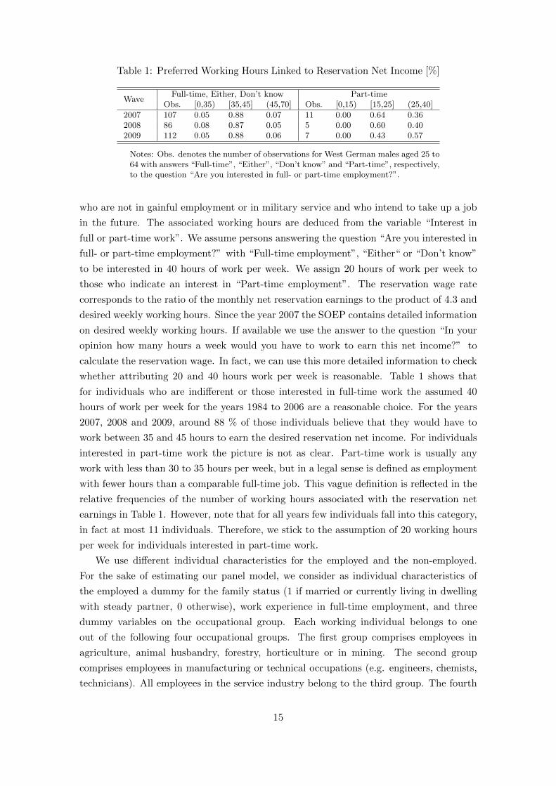
Table 1: Preferred Working Hours Linked to Reservation Net Income [%]

WaveFull-time, Either, Don’t know Part-time

Obs. [0,35) [35,45] (45,70] Obs. [0,15) [15,25] (25,40]

2007 107 0.05 0.88 0.07 11 0.00 0.64 0.362008 86 0.08 0.87 0.05 5 0.00 0.60 0.402009 112 0.05 0.88 0.06 7 0.00 0.43 0.57

Notes: Obs. denotes the number of observations for West German males aged 25 to64 with answers “Full-time”, “Either”, “Don’t know” and “Part-time”, respectively,to the question “Are you interested in full- or part-time employment?”.

who are not in gainful employment or in military service and who intend to take up a job

in the future. The associated working hours are deduced from the variable “Interest in

full or part-time work”. We assume persons answering the question “Are you interested in

full- or part-time employment?” with “Full-time employment”, “Either“ or “Don’t know”

to be interested in 40 hours of work per week. We assign 20 hours of work per week to

those who indicate an interest in “Part-time employment”. The reservation wage rate

corresponds to the ratio of the monthly net reservation earnings to the product of 4.3 and

desired weekly working hours. Since the year 2007 the SOEP contains detailed information

on desired weekly working hours. If available we use the answer to the question “In your

opinion how many hours a week would you have to work to earn this net income?” to

calculate the reservation wage. In fact, we can use this more detailed information to check

whether attributing 20 and 40 hours work per week is reasonable. Table 1 shows that

for individuals who are indifferent or those interested in full-time work the assumed 40

hours of work per week for the years 1984 to 2006 are a reasonable choice. For the years

2007, 2008 and 2009, around 88 % of those individuals believe that they would have to

work between 35 and 45 hours to earn the desired reservation net income. For individuals

interested in part-time work the picture is not as clear. Part-time work is usually any

work with less than 30 to 35 hours per week, but in a legal sense is defined as employment

with fewer hours than a comparable full-time job. This vague definition is reflected in the

relative frequencies of the number of working hours associated with the reservation net

earnings in Table 1. However, note that for all years few individuals fall into this category,

in fact at most 11 individuals. Therefore, we stick to the assumption of 20 working hours

per week for individuals interested in part-time work.

We use different individual characteristics for the employed and the non-employed.

For the sake of estimating our panel model, we consider as individual characteristics of

the employed a dummy for the family status (1 if married or currently living in dwelling

with steady partner, 0 otherwise), work experience in full-time employment, and three

dummy variables on the occupational group. Each working individual belongs to one

out of the following four occupational groups. The first group comprises employees in

agriculture, animal husbandry, forestry, horticulture or in mining. The second group

comprises employees in manufacturing or technical occupations (e.g. engineers, chemists,

technicians). All employees in the service industry belong to the third group. The fourth

15

group comprises all other workers, in particular persons who do not report an established

profession or workers without any further specification of their professional activity.

As mentioned in section 4 we use an IV approach to account for the possible endogene-

ity of wages. Following the ideas of Mincer (1974) who viewed wages as predominantly

determined by accumulated human capital, we include as instruments schooling, work ex-

perience in full-time employment, and work experience squared. The schooling variable

is based on the number of years of education or training undergone and exhibits some

variation over time. It includes secondary vocational education and ranges from 7 to 18

years.13

The determinants of the reservation wage which are needed for the estimation of the

conditional density f twR|X(·) are given by unemployment experience in years, a dummy

on whether or not information for unemployment benefits is provided, the size of unem-

ployment benefits, and a dummy for highly qualified individuals. The latter group has

obtained a college or university degree.14 Note that in each year individuals are asked

about the size of the unemployment benefits in the previous year so that the information

about unemployment benefits is not available for the last wave, i.e. 2009. For estimating

f tw|X(·) we use schooling, work experience in full-time employment, and work experience

squared.

6 Results

We start this section by presenting results from the panel, density and conditional expecta-

tion estimation needed for the determination of the total adjustments along the intensive

and extensive margin, respectively. Then, we provide results for the aggregate Frisch

wage-elasticity of labor supply.

6.1 Panel model estimation

For calculating the total labor supply adjustment along the intensive margin τ inth,t , we first

have to estimate the panel data model for the working population. Results for the first

stage of the panel model estimation are given in Table 7 in Appendix E. All instruments

and the constant are highly significant. Wage rates rise in the years of schooling and in

work experience gathered. However, the coefficient on work experience squared is negative,

so that each further increase in experience conveys a progressively smaller increase in the

wage rate.

Table 2 shows results for the panel model estimation, equation (26). For the benchmark

specification, i.e. the IV approach, the coefficient on the family status dummy variable is

13There exist alternative instruments, e.g., a regionally varying unemployment rate which is availablefrom IAB (German Bureau of Labor Statistics), Nuremberg.

14These determinants of the reservation wage rate are in line with the literature as Prasad (2004) andAddison et al. (2009), among others, find that duration of joblessness, availability and level of unemploy-ment compensation and observables of education or skill level are the most important determinants ofreservation wages.

16

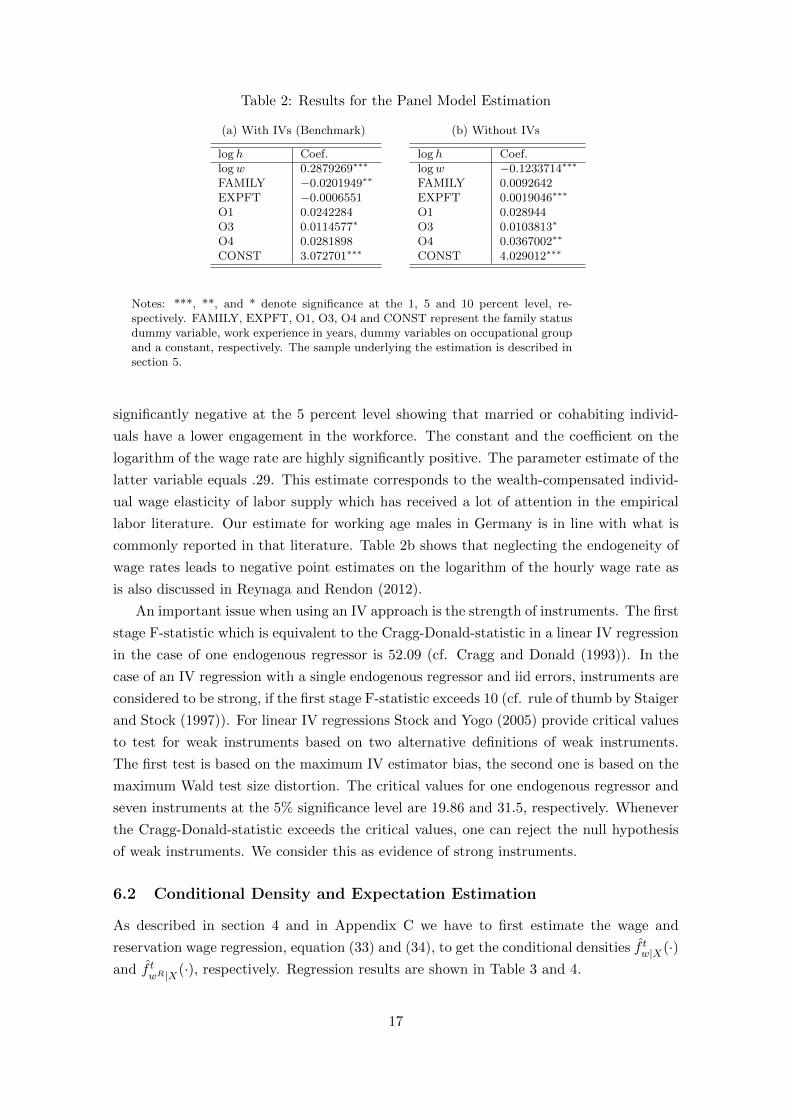
Table 2: Results for the Panel Model Estimation

(a) With IVs (Benchmark)

log h Coef.logw 0.2879269∗∗∗

FAMILY −0.0201949∗∗

EXPFT −0.0006551O1 0.0242284O3 0.0114577∗

O4 0.0281898CONST 3.072701∗∗∗

(b) Without IVs

log h Coef.logw −0.1233714∗∗∗

FAMILY 0.0092642EXPFT 0.0019046∗∗∗

O1 0.028944O3 0.0103813∗

O4 0.0367002∗∗

CONST 4.029012∗∗∗

Notes: ***, **, and * denote significance at the 1, 5 and 10 percent level, re-spectively. FAMILY, EXPFT, O1, O3, O4 and CONST represent the family statusdummy variable, work experience in years, dummy variables on occupational groupand a constant, respectively. The sample underlying the estimation is described insection 5.

significantly negative at the 5 percent level showing that married or cohabiting individ-

uals have a lower engagement in the workforce. The constant and the coefficient on the

logarithm of the wage rate are highly significantly positive. The parameter estimate of the

latter variable equals .29. This estimate corresponds to the wealth-compensated individ-

ual wage elasticity of labor supply which has received a lot of attention in the empirical

labor literature. Our estimate for working age males in Germany is in line with what is

commonly reported in that literature. Table 2b shows that neglecting the endogeneity of

wage rates leads to negative point estimates on the logarithm of the hourly wage rate as

is also discussed in Reynaga and Rendon (2012).

An important issue when using an IV approach is the strength of instruments. The first

stage F-statistic which is equivalent to the Cragg-Donald-statistic in a linear IV regression

in the case of one endogenous regressor is 52.09 (cf. Cragg and Donald (1993)). In the

case of an IV regression with a single endogenous regressor and iid errors, instruments are

considered to be strong, if the first stage F-statistic exceeds 10 (cf. rule of thumb by Staiger

and Stock (1997)). For linear IV regressions Stock and Yogo (2005) provide critical values

to test for weak instruments based on two alternative definitions of weak instruments.

The first test is based on the maximum IV estimator bias, the second one is based on the

maximum Wald test size distortion. The critical values for one endogenous regressor and

seven instruments at the 5% significance level are 19.86 and 31.5, respectively. Whenever

the Cragg-Donald-statistic exceeds the critical values, one can reject the null hypothesis

of weak instruments. We consider this as evidence of strong instruments.

6.2 Conditional Density and Expectation Estimation

As described in section 4 and in Appendix C we have to first estimate the wage and

reservation wage regression, equation (33) and (34), to get the conditional densities f tw|X(·)and f t

wR|X(·), respectively. Regression results are shown in Table 3 and 4.

17

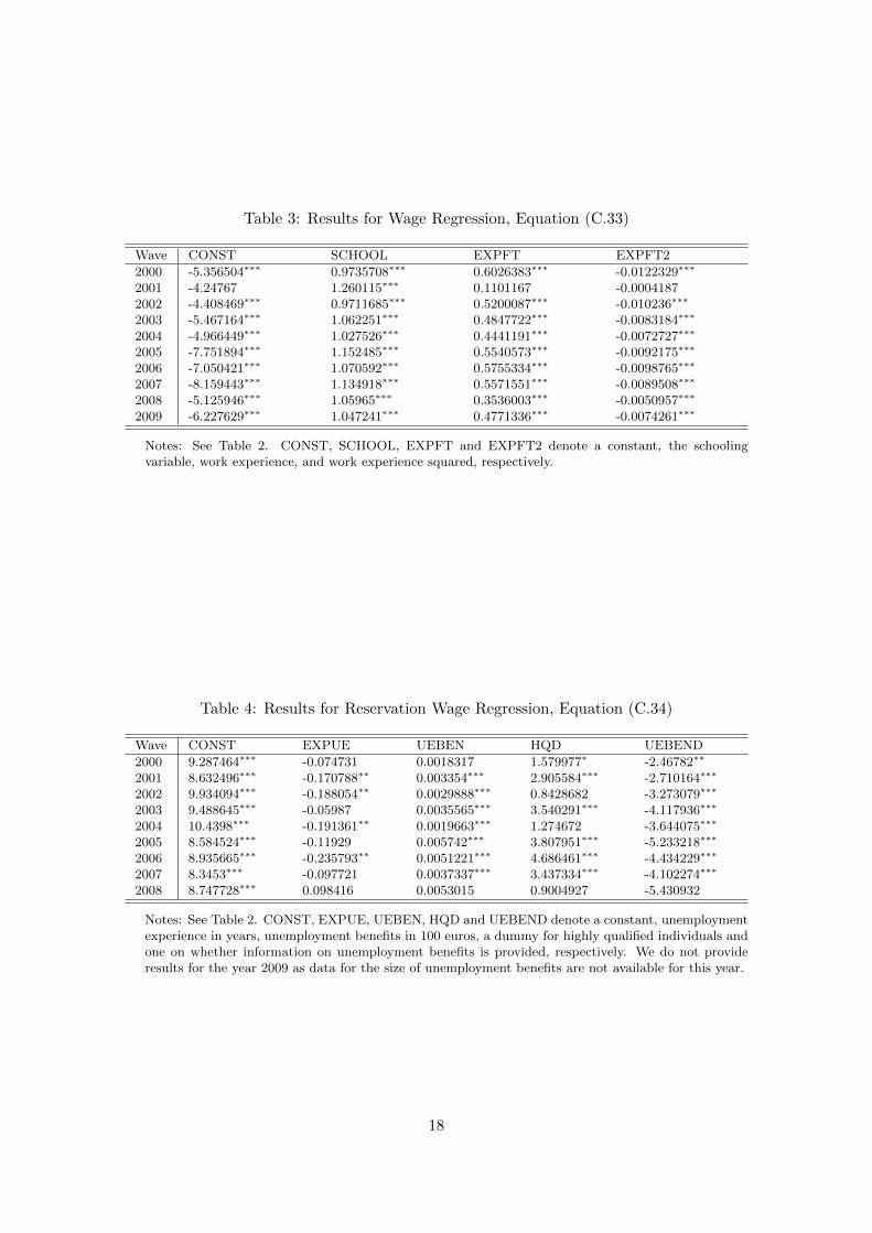
Table 3: Results for Wage Regression, Equation (C.33)

Wave CONST SCHOOL EXPFT EXPFT2

2000 -5.356504∗∗∗ 0.9735708∗∗∗ 0.6026383∗∗∗ -0.0122329∗∗∗

2001 -4.24767 1.260115∗∗∗ 0.1101167 -0.00041872002 -4.408469∗∗∗ 0.9711685∗∗∗ 0.5200087∗∗∗ -0.010236∗∗∗

2003 -5.467164∗∗∗ 1.062251∗∗∗ 0.4847722∗∗∗ -0.0083184∗∗∗

2004 -4.966449∗∗∗ 1.027526∗∗∗ 0.4441191∗∗∗ -0.0072727∗∗∗

2005 -7.751894∗∗∗ 1.152485∗∗∗ 0.5540573∗∗∗ -0.0092175∗∗∗

2006 -7.050421∗∗∗ 1.070592∗∗∗ 0.5755334∗∗∗ -0.0098765∗∗∗

2007 -8.159443∗∗∗ 1.134918∗∗∗ 0.5571551∗∗∗ -0.0089508∗∗∗

2008 -5.125946∗∗∗ 1.05965∗∗∗ 0.3536003∗∗∗ -0.0050957∗∗∗

2009 -6.227629∗∗∗ 1.047241∗∗∗ 0.4771336∗∗∗ -0.0074261∗∗∗

Notes: See Table 2. CONST, SCHOOL, EXPFT and EXPFT2 denote a constant, the schoolingvariable, work experience, and work experience squared, respectively.

Table 4: Results for Reservation Wage Regression, Equation (C.34)

Wave CONST EXPUE UEBEN HQD UEBEND

2000 9.287464∗∗∗ -0.074731 0.0018317 1.579977∗ -2.46782∗∗

2001 8.632496∗∗∗ -0.170788∗∗ 0.003354∗∗∗ 2.905584∗∗∗ -2.710164∗∗∗

2002 9.934094∗∗∗ -0.188054∗∗ 0.0029888∗∗∗ 0.8428682 -3.273079∗∗∗

2003 9.488645∗∗∗ -0.05987 0.0035565∗∗∗ 3.540291∗∗∗ -4.117936∗∗∗

2004 10.4398∗∗∗ -0.191361∗∗ 0.0019663∗∗∗ 1.274672 -3.644075∗∗∗

2005 8.584524∗∗∗ -0.11929 0.005742∗∗∗ 3.807951∗∗∗ -5.233218∗∗∗

2006 8.935665∗∗∗ -0.235793∗∗ 0.0051221∗∗∗ 4.686461∗∗∗ -4.434229∗∗∗

2007 8.3453∗∗∗ -0.097721 0.0037337∗∗∗ 3.437334∗∗∗ -4.102274∗∗∗

2008 8.747728∗∗∗ 0.098416 0.0053015 0.9004927 -5.430932

Notes: See Table 2. CONST, EXPUE, UEBEN, HQD and UEBEND denote a constant, unemploymentexperience in years, unemployment benefits in 100 euros, a dummy for highly qualified individuals andone on whether information on unemployment benefits is provided, respectively. We do not provideresults for the year 2009 as data for the size of unemployment benefits are not available for this year.

18

As is the case for the first stage of the panel model estimation, for all years except for

2001 the coefficients on the individual characteristics as well as the constant are highly

significant. Wage rates rise in the years of schooling and in work experience gathered.

However, the coefficient on work experience squared is negative, so that each further

increase in experience conveys a progressively smaller increase in the wage rate.

For the estimation of equation (C.34) we have between 91 and 140 observations and the

constant is highly significant between 8.35 and 10.44. The coefficient on the unemployment

duration is mostly negative and not significant. The predominant sign of the coefficient is

in line with predictions from theoretical models and empirical evidence that the reservation

wage decreases with waiting time for a new job. The reservation wage rate significantly

decreases if non-employed individuals receive unemployment benefits, but they increase in

the level of those benefits. Being a highly qualified individual, i.e. having obtained a college

or university degree, increases the reservation wage, in most cases (highly) significantly.

The resulting conditional densities f tw|X(·) and f twR|X(·) vary with individual charac-

teristics X = Xit. Therefore, we restrict our analysis to the densities conditional on mean

individual characteristics, i.e. Xit = Xt. Note that this choice is rather arbitrary. One

could also consider results for median or prespecified individual characteristics. Figure

1 shows the lower quartile, the median and the upper quartile for the wage as well as

the reservation wage distribution conditional on mean individual characteristics. It does

not come as a surprise that the distribution of the reservation wage is left of the wage

distribution for all years as individuals are only working if the offered wage exceeds the

reservation wage. For the wage distribution, the lower quartile, the median and the upper

quartile vary around 10.3, 12.9 and 15.8, respectively. For 2001 the distribution is more

dispersed which is possibly also one reason for the less accurate regression results in this

year. On the other hand, for the reservation wage distribution, the lower quartile, the

median and the upper quartile vary around 7.7, 9.5 and 11.4, respectively. In 2008, the

distribution shifts slightly to the left which probably is the result of a decrease in the mean

size of unemployment benefits which have a negative influence on reservation wage rates.

In the following, we consider results from the conditional expectation estimation gen-

erated by considering the reservation wage wR and associated hours data hR for each year.

Figure 2 shows the nonparametric regression results for all years. The expectation corre-

sponds to the hours a marginal worker would work at her reservation wage. Therefore,

the estimated values of around 40 working hours per week seem plausible.

6.3 The Aggregate Frisch Wage-Elasticity of Labor Supply

For the calculation of the aggregate Frisch elasticity we determine the employment ratio

EPRt, the mean labor supply Ht as well as the mean wage rate W t received by all

working individuals directly from observed data (see Table 8 in Appendix E). Results for

the estimated determinants of the aggregate Frisch wage-elasticity, i.e. τ inth,t , τ exth,t and τ extw,t

19

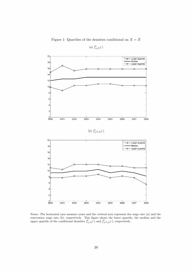
Figure 1: Quartiles of the densities conditional on X = X

(a) f tw|X(·)

(b) f twR|X(·)

Notes: The horizontal axes measure years and the vertical axes represent the wage rate (a) and thereservation wage rate (b), respectively. This figure shows the lower quartile, the median and theupper quartile of the conditional densities f tw|X(·) and f twR|X(·), respectively.

20

Figure 2: Expectation of weekly working hours conditional on w = wR

Notes: The horizontal axis measures the real hourly wage rate and the vertical axis represents workinghours. This figure shows the regression functions for the conditional expectation E(ht| wRt = wt) forthe years 2000 to 2009.

are shown in Table 9 in Appendix E whereas results for the aggregate Frisch wage-elasticity

et =W t

Ht

(τ inth,t + τ exth,t

EPRt + τ extw,t

)

=W t

Ht

1

EPRt + τ extw,t

· τ inth,t︸ ︷︷ ︸τ inth,t

+W t

Ht

1

EPRt + τ extw,t

· τ exth,t︸ ︷︷ ︸τexth,t

.

and its weighted components τ inth,t and τ exth,t are shown in Table 5. The aggregate Frisch

elasticity ranges from .63 in 2008 to .70 in 2003 and 2004. Considering only the first eight

years from 2000 to 2007, the aggregate Frisch elasticity varies very little between .68 and

.70. The slightly lower value of 0.63 in 2008 is caused by the lower hours adjustment along

the extensive margin, i.e. a lower value of τ exth,t in 2008 compared to the other years. Our

estimates of the aggregate elasticity is very close to what Fiorito and Zanella (2012) report

for continuously employed men in the US. Table 5 also shows that about one third of the

aggregate adjustment is due to hours adjustment of stayers and the remaining two-thirds

are due to hours worked by new entrants into the labor market.

7 Conclusion

This paper illustrates the power and the importance of taking statistical aggregation seri-

ously when thinking about possible links between individual and aggregate Frisch wage-

elasticities of labor supply in an environment where workers are heterogenous. Statistical

aggregation introduces non-linearities which drive a wedge between the mean of individual

21

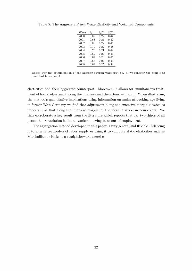
Table 5: The Aggregate Frisch Wage-Elasticity and Weighted Components

Wave et τ inth,t τexth,t

2000 0.69 0.22 0.472001 0.68 0.27 0.422002 0.68 0.22 0.462003 0.70 0.22 0.482004 0.70 0.21 0.492005 0.69 0.24 0.452006 0.69 0.23 0.462007 0.68 0.24 0.452008 0.63 0.25 0.38

Notes: For the determination of the aggregate Frisch wage-elasticity et we consider the sample asdescribed in section 5.

elasticities and their aggregate counterpart. Moreover, it allows for simultaneous treat-

ment of hours adjustment along the intensive and the extensive margin. When illustrating

the method’s quantitative implications using information on males at working-age living

in former West-Germany we find that adjustment along the extensive margin is twice as

important as that along the intensive margin for the total variation in hours work. We

thus corroborate a key result from the literature which reports that ca. two-thirds of all

person hours variation is due to workers moving in or out of employment.

The aggregation method developed in this paper is very general and flexible. Adapting

it to alternative models of labor supply or using it to compute static elasticities such as

Marshallian or Hicks is a straightforward exercise.

22

References

Addison, J. T., Centeno, M., and Portugal, P. (2009). Do reservation wages really decline?

Some international evidence on the determinants of reservation wages. Journal of Labor

Research, 30:1–8.

Altonji, J. G. (1986). Intertemporal substitution in labor supply: Evidence from micro

data. Journal of Political Economy, 94(3):176–215.

Blundell, R. and MaCurdy, T. (1999). Labor supply: A review of alternative approaches.

In Ashenfelter, O. and Card, D., editors, Handbook of Labor Economics, volume 3, pages

1559–1695. Elsevier, Amsterdam: North-Holland.

Chang, Y. and Kim, S.-B. (2005). On the aggregate labor supply. Economic Quarterly,

Winter:21–37. Federal Reserve Bank of Richmond.

Chang, Y. and Kim, S.-B. (2006). From individual to aggregate labor supply: A quanti-

tative analysis based on a heterogeneous agent macroeconomy. International Economic

Review, 47(1):1–27.

Chetty, R., Guren, A., Manoli, D., and Weber, A. (2012). Does indivisible labor explain the

difference between micro and macro elasticities? A meta-analysis of extensive margin

elasticities. In NBER Macroeconomics Annual, volume 27, pages 1–56. National Bureau

of Economic Research, Inc.

Cragg, J. G. and Donald, S. G. (1993). Testing identifiability and specification in instru-

mental variable models. Econometric Theory, 9(2):222–240.

Fiorito, R. and Zanella, G. (2012). The anatomy of the aggregate labor supply elasticity.

Review of Economic Dynamics, 15(2):171–187.

Gourio, F. and Noual, P.-A. (2009). The marginal worker and the aggregate elasticity of

labor supply. Discussion paper, Boston University.

Hall, R. E. (2012). Viewing job-seekers’ reservation wages and acceptance decisions

through the lens of search theory. Working paper, Stanford University.

Hansen, G. D. (1985). Indivisible labor and the business cycle. Journal of Monetary

Economics, 16(3):309–327.

Hildenbrand, W. and Kneip, A. (2005). Aggregate behavior and microdata. Games and

Economic Behavior, 50(1):3–27.

Li, Q. and Racine, J. S. (2006). Nonparametric Econometrics: Theory and Practice,

volume 1. Economics Books, Princeton University Press.

Lucas, R. E. J. and Rapping, L. A. (1969). Real wages, employment, and inflation. Journal

of Political Economy, 77(5):721–54.

23

MaCurdy, T. (1981). An empirical model of labor supply in a life-cycle setting. Journal

of Political Economy, 89(6):1059–1085.

MaCurdy, T. (1985). Interpreting empirical models of labor supply in an intertempo-

ral framework with uncertainty. In Heckman, J. and Singer, B., editors, Longitudinal

analysis of labour market data. Cambridge University Press, Cambridge UK.

Mincer, J. (1974). Schooling, Experience and Earnings. Columbia University Press, New

York.

Nadaraya, E. A. (1964). On estimating regression. Theory of Probability and Its Applica-

tions, 9(1):141–142.

Paluch, M., Kneip, A., and Hildenbrand, W. (2012). Individual versus aggregate income

elasticities for heterogeneous populations. Journal of Applied Econometrics, 27(5):847–

869.

Prasad, E. S. (2004). What Determines the Reservation Wages of Unemployed Workers?

New Evidence from German Micro Data. Institutions and Wage Formation in the New

Europe: Proceedings of the ECB’s Annual Labor Market Workshop. Edward Elgar,

London.

Reynaga, N. C. and Rendon, S. (2012). The frisch elasticity in labor markets with high

job turnover. Department of Economics Working Papers 12-13, Stony Brook University.

Rogerson, R. (1988). Indivisible labor, lotteries and equilibrium. Journal of Monetary

Economics, 21(1):3–16.

Staiger, D. and Stock, J. H. (1997). Instrumental variables regression with weak instru-

ments. Econometrica, 65(3):557–586.

Stock, J. and Yogo, M. (2005). Testing for Weak Instruments in Linear IV Regression,

pages 80–108. In Identification and Inference for Econometric Models: Essays in Honor

of Thomas Rothenberg, ed. D.W. Andrews and J. H. Stock. Cambridge University Press,

Cambridge UK.

Watson, G. S. (1964). Smooth regression analysis. Sankhya: The Indian Journal of

Statistics, Series A, 26(4):359–372.

24

Appendix A Aggregate Frisch elasticities under monotone

transformations

An aggregate Frisch wage-elasticity can be derived for any smooth, strictly monotone

transformation wt → T (∆, wt) with T (0, wt) = wt of wages. Given such a transformation,

(15a) and (15b) generalize to

Ht;T (∆) :=

∫g(T (∆, w), λ, Y )I(T (∆, w) ≥ wR)dπtw,wR,λ,Y ,

W t;T (∆) :=

∫T (∆, w)I(T (∆, w) ≥ wR)dπtw,wR .

By (16), determining a Frisch wage-elasticity et;T then requires to calculate the derivatives

of W t;T (∆) and Ht;T (∆) at ∆ = 0. Let T ∗(w) = ∂T (∆,w)∂∆

∣∣∣∣∆=0

. If T (∆, w) = w + ∆

then T ∗(w) ≡ 1. For proportional changes T (∆, w) = w(1 + ∆) we have T ∗(w) = w.

Straightforward generalizations of the arguments leading to (18) and (20) then yield

∂W t;T (∆)

∂∆

∣∣∣∣∆=0

=

∫T ∗(w)I(w ≥ wR)dπtw,wR︸ ︷︷ ︸

τ intw,t;T

+

∫νT ∗(ν)f twR|ν(ν)f tw(ν)dν︸ ︷︷ ︸

τextw,t;T

,

∂Ht;T (∆)

∂∆

∣∣∣∣∆=0

=

∫T ∗(w)∂wg(w, λ, Y )I(w ≥ wR)dπtw,wR,λ,Y︸ ︷︷ ︸

τ inth,t;T

+

∫E(ht| wRt = wt = ν

)T ∗(ν)f twR|ν(ν)f tw(ν)dν︸ ︷︷ ︸

τexth,t;T

,

The aggregate Frisch wage-elasticity et;T with respect to the transformation T is given by

et;T =W t

Ht

(τ inth,t;T + τ exth,t;T

τ intw,t;T + τ extw,t;T

).

Appendix B Formal derivation of the derivative of equation

(19), second term

We obtain∫g(w + ∆, λ, Y )I(wR ∈ [w,w + ∆])dπtw,wR,λ,Y

=

∫ ∫ ∫g(w + ∆, λ, Y )dπt(λ,Y )|(wR,w)I(wR ∈ [w,w + ∆])dπtwR|wdπ

tw

=

∫ (∫ ν+∆

ν

E(g(wt + ∆, λt, Yt)| wRt = ν, wt = ν

)f twR|ν(ν)dν

)f tw(ν)dν.

25

In what follows we assume the conditional expectation E(g(wt+ ∆, λt, Yt)| wRt = ν, wt =

ν

)as well as f t

wR|ν(ν) to be continuous functions of ν and ν. Also note that E(g(wt, λt, Yt)| wRt =

wt = ν

)= E

(ht| wRt = wt = ν

). The mean value theorem then implies that for all ν

there exist a ξν ∈ [ν, ν + ∆] such that

∫ (∫ ν+∆

ν

E(g(wt + ∆, λt, Yt)| wRt = ν, wt = ν

)f twR|ν(ν)dν

)f tw(ν)dν

=

∫∆E(g(wt + ∆, λt, Yt)| wRt = ξν , wt = ν

)f twR|ν(ξν)f tw(ν)dν

=∆

∫E(ht| wRt = wt = ν

)f twR|ν(ν)f tw(ν)dν

+ ∆

∫ (E(g(wt + ∆, λt, Yt)| wRt = ξν , wt = ν

)f twR|ν(ξν)

− E(g(wt, λt, Yt)| wRt = wt = ν

)f twR|ν(ν)

)f tw(ν)dν.

Obviously, for all ν,∣∣∣∣E(g(wt + ∆, λt, Yt)| wRt = ξν , wt = ν

)f twR|ν(ξν)− E

(g(wt, λt, Yt)| wRt = wt = ν

)f twR|ν(ν)

∣∣∣∣→ 0

as ∆→ 0. Therefore,

∂

∂∆

∫g(w + ∆, λt, Y )I(wR ∈ [w,w + ∆])dπtw,wR,λ,Y

∣∣∣∣∆=0

= lim∆→0

∫g(w + ∆, λt, Y )I(wR ∈ [w,w + ∆])dπtw,wR,λ,Y

∆

=

∫E(ht| wRt = wt = ν

)f twR|ν(ν)f tw(ν)dν.

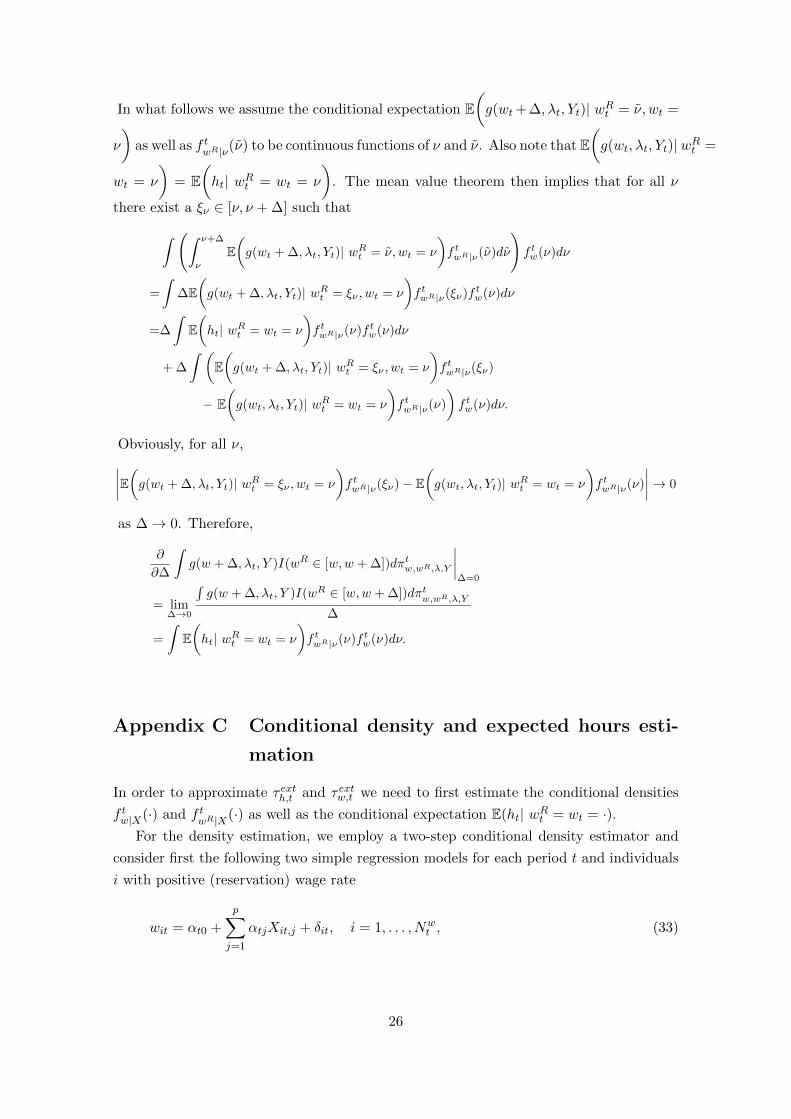
Appendix C Conditional density and expected hours esti-

mation

In order to approximate τ exth,t and τ extw,t we need to first estimate the conditional densities

f tw|X(·) and f twR|X(·) as well as the conditional expectation E(ht| wRt = wt = ·).

For the density estimation, we employ a two-step conditional density estimator and

consider first the following two simple regression models for each period t and individuals

i with positive (reservation) wage rate

wit = αt0 +

p∑j=1

αtjXit,j + δit, i = 1, . . . , Nwt , (33)

26

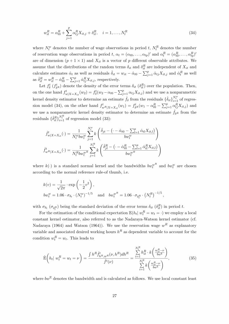
wRit = αRt0 +

p∑j=1

αRtjXit,j + δRit , i = 1, . . . , NRt (34)

where Nwt denotes the number of wage observations in period t, NR

t denotes the number

of reservation wage observations in period t, αt = (αt0, . . . , αtp)′ and αRt = (αRt0, . . . , α

Rtp)′

are of dimension (p + 1 × 1) and Xit is a vector of p different observable attributes. We

assume that the distributions of the random terms δit and δRit are independent of Xit and

calculate estimates αt as well as residuals δit = wit − αt0 −∑p

j=1 αtjXit,j and αRt as well

as δRit = wRit − αRt0 −∑p

j=1 αRtjXit,j , respectively.

Let f tδ (f tδR

) denote the density of the error terms δit (δRit ) over the population. Then,

on the one hand f tw|X=Xit(w2) = f tδ(w2−αt0−

∑pj=1 αtjXit,j) and we use a nonparametric

kernel density estimator to determine an estimate fδ from the residuals {δit}Nwt

i=1 of regres-

sion model (34), on the other hand f twR|X=Xit

(w1) = f tδR

(w1 − αRt0 −∑p

j=1 αRtjXit,j) and

we use a nonparametric kernel density estimator to determine an estimate fδR from the

residuals {δRit}NRt

i=1 of regression model (33):

f tw|X=Xit(·) =

1

Nwt bw

wt

Nwt∑

j=1

k

(δjt −

(· − αt0 −

∑pl=1 αtlXit,l

)bwwt

)

f twR|X=Xit(·) =

1

NRt bw

wRt

NRt∑

j=1

k

(δRjt −

(· − αRt0 −

∑pl=1 α

RtlXit,l

)bww

R

t

)

where k(·) is a standard normal kernel and the bandwidths bwwR

t and bwwt are chosen

according to the normal reference rule-of thumb, i.e.

k(v) =1√2π· exp

(−1

2v2

),

bwwt = 1.06 · σδt · (Nwt )−1/5 and bww

R

t = 1.06 · σδRt ·(NRt

)−1/5,

with σδt (σδRt ) being the standard deviation of the error terms δit (δRit ) in period t.

For the estimation of the conditional expectation E(ht| wRt = wt = ·) we employ a local

constant kernel estimator, also referred to as the Nadaraya-Watson kernel estimator (cf.

Nadaraya (1964) and Watson (1964)). We use the reservation wage wR as explanatory

variable and associated desired working hours hR as dependent variable to account for the

condition wRt = wt. This leads to

E(ht| wRt = wt = ν

)=

∫hRf t

hR,wR(ν, hR)dhR

f t(ν)=

NRt∑

i=1hRit · k

(wRit−νbwE

)NRt∑

i=1k

(wRit−νbwE

) , (35)

where bwE denotes the bandwidth and is calculated as follows. We use local constant least

27

squares cross-validation with leave-one-out kernel estimator to calculate the smoothing

parameter for each year. Then, the bandwidth bwE is the average over all smoothing

parameters.

Appendix D Data

D.1 SOEP Samples

Each household and thereby each individual in the SOEP is part of one of the following

samples:

• Sample A: ‘Residents in the FRG’, started 1984

• Sample B: ‘Foreigners in the FRG’, started 1984

• Sample C: ‘German Residents in the GDR’, started 1990

• Sample D: ‘Immigrants’, started 1994/95

• Sample E: ‘Refreshment’, started 1998

• Sample F: ‘Innovation’, started 2000

• Sample G: ‘Oversampling of High Income’, started 2002

• Sample H: ‘Extension’, started 2006

• Sample I: ‘Incentivation’, started 2009

28

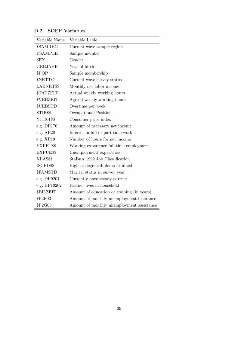
D.2 SOEP Variables

Variable Name Variable Lable

$SAMREG Current wave sample region

PSAMPLE Sample member

SEX Gender

GEBJAHR Year of birth

$POP Sample membership

$NETTO Current wave survey status

LABNET$$ Monthly net labor income

$TATZEIT Actual weekly working hours

$VEBZEIT Agreed weekly working hours

$UEBSTD Overtime per week

STIB$$ Occupational Position

Y11101$$ Consumer price index

e.g. DP170 Amount of necessary net income

e.g. AP20 Interest in full or part-time work

e.g. XP19 Number of hours for net income

EXPFT$$ Working experience full-time employment

EXPUE$$ Unemployment experience

KLAS$$ StaBuA 1992 Job Classification

ISCED$$ Highest degree/diploma attained

$FAMSTD Marital status in survey year

e.g. DP9201 Currently have steady partner

e.g. HP10202 Partner lives in household

$BILZEIT Amount of education or training (in years)

$P2F03 Amount of monthly unemployment insurance

$P2G03 Amount of monthly unemployment assistance

29

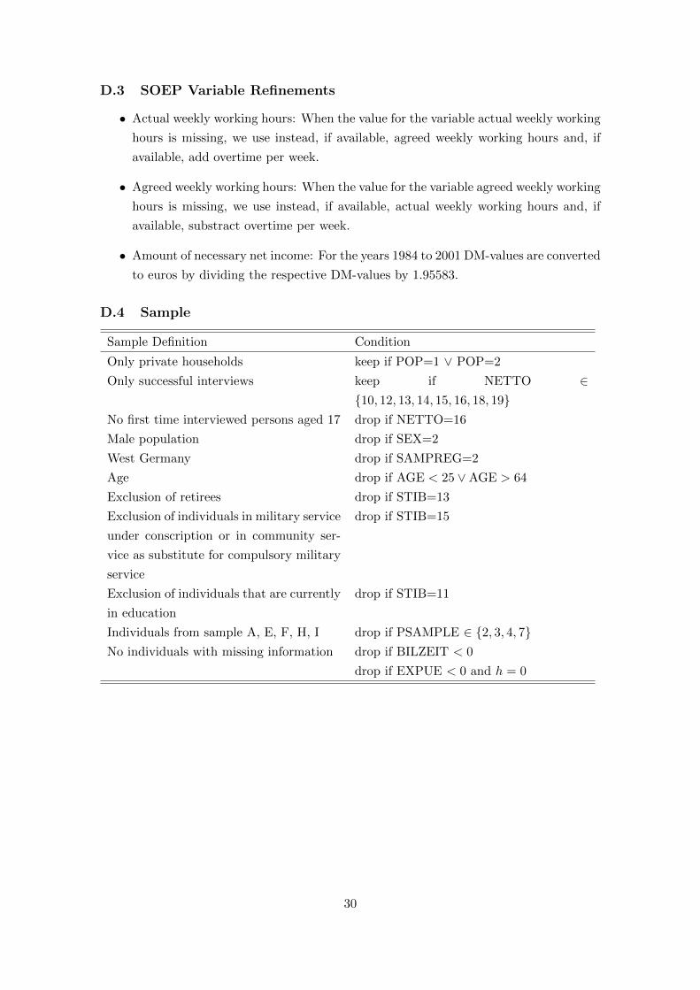
D.3 SOEP Variable Refinements

• Actual weekly working hours: When the value for the variable actual weekly working

hours is missing, we use instead, if available, agreed weekly working hours and, if

available, add overtime per week.

• Agreed weekly working hours: When the value for the variable agreed weekly working

hours is missing, we use instead, if available, actual weekly working hours and, if

available, substract overtime per week.

• Amount of necessary net income: For the years 1984 to 2001 DM-values are converted

to euros by dividing the respective DM-values by 1.95583.

D.4 Sample

Sample Definition Condition

Only private households keep if POP=1 ∨ POP=2

Only successful interviews keep if NETTO ∈{10, 12, 13, 14, 15, 16, 18, 19}

No first time interviewed persons aged 17 drop if NETTO=16

Male population drop if SEX=2

West Germany drop if SAMPREG=2

Age drop if AGE < 25 ∨AGE > 64

Exclusion of retirees drop if STIB=13

Exclusion of individuals in military service

under conscription or in community ser-

vice as substitute for compulsory military

service

drop if STIB=15

Exclusion of individuals that are currently

in education

drop if STIB=11

Individuals from sample A, E, F, H, I drop if PSAMPLE ∈ {2, 3, 4, 7}No individuals with missing information drop if BILZEIT < 0

drop if EXPUE < 0 and h = 0

30

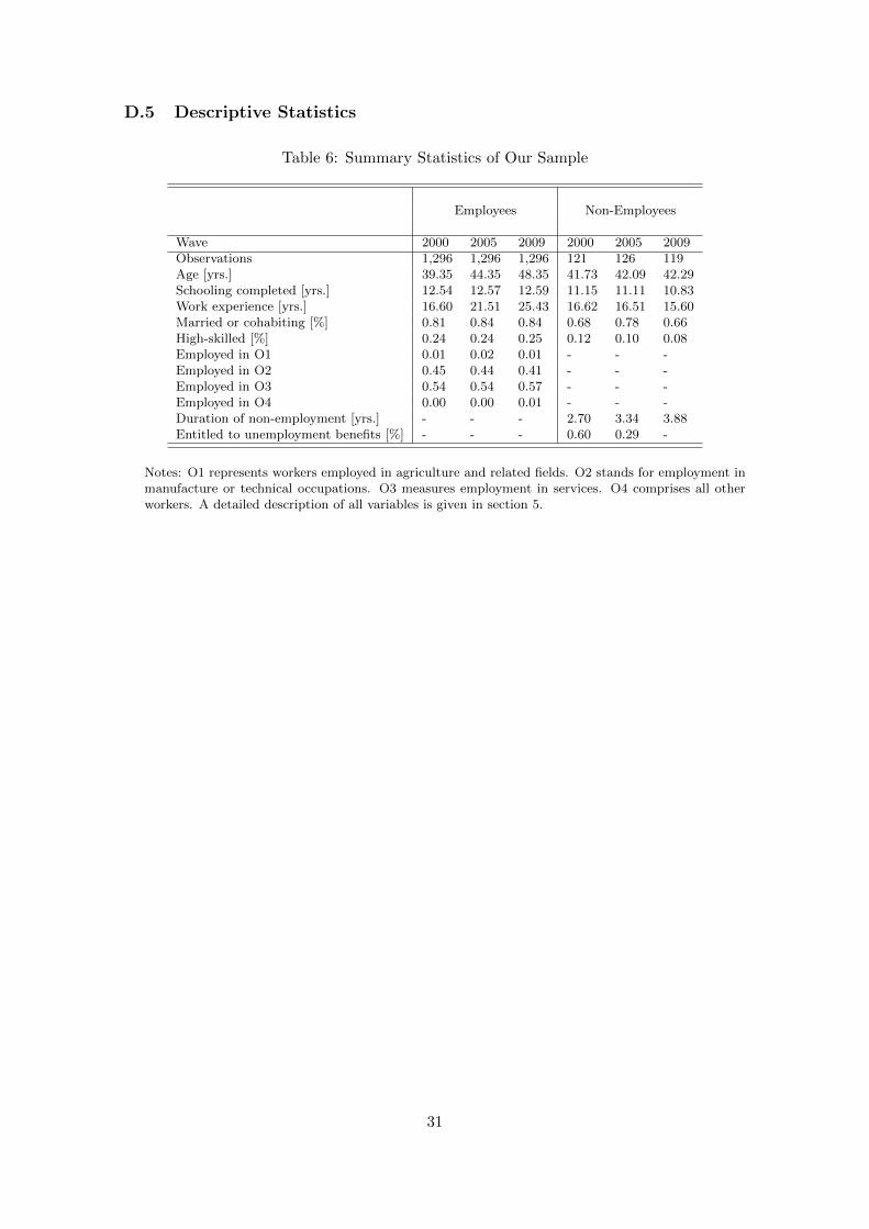
D.5 Descriptive Statistics

Table 6: Summary Statistics of Our Sample

Employees Non-Employees

Wave 2000 2005 2009 2000 2005 2009Observations 1,296 1,296 1,296 121 126 119Age [yrs.] 39.35 44.35 48.35 41.73 42.09 42.29Schooling completed [yrs.] 12.54 12.57 12.59 11.15 11.11 10.83Work experience [yrs.] 16.60 21.51 25.43 16.62 16.51 15.60Married or cohabiting [%] 0.81 0.84 0.84 0.68 0.78 0.66High-skilled [%] 0.24 0.24 0.25 0.12 0.10 0.08Employed in O1 0.01 0.02 0.01 - - -Employed in O2 0.45 0.44 0.41 - - -Employed in O3 0.54 0.54 0.57 - - -Employed in O4 0.00 0.00 0.01 - - -Duration of non-employment [yrs.] - - - 2.70 3.34 3.88Entitled to unemployment benefits [%] - - - 0.60 0.29 -

Notes: O1 represents workers employed in agriculture and related fields. O2 stands for employment inmanufacture or technical occupations. O3 measures employment in services. O4 comprises all otherworkers. A detailed description of all variables is given in section 5.

31

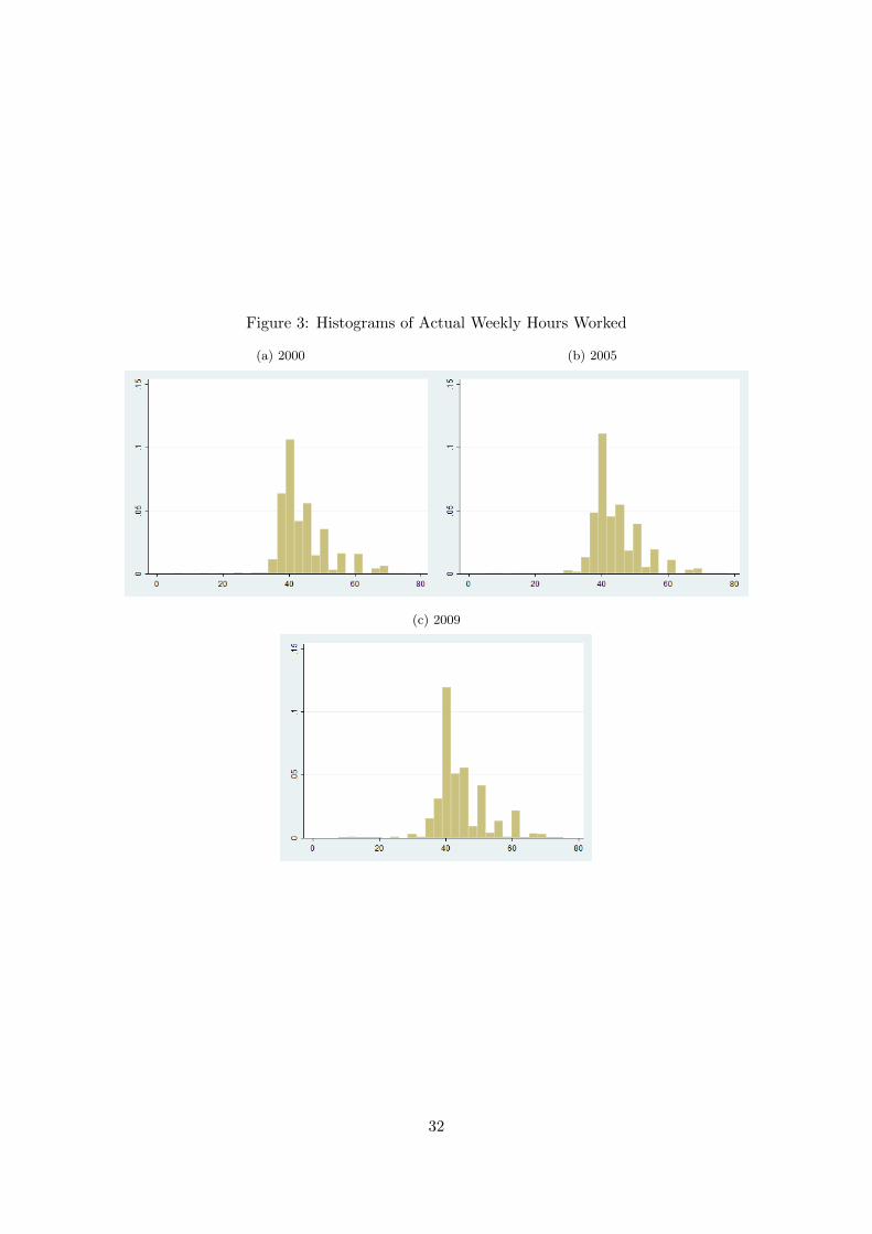
Figure 3: Histograms of Actual Weekly Hours Worked

(a) 2000 (b) 2005

(c) 2009

32

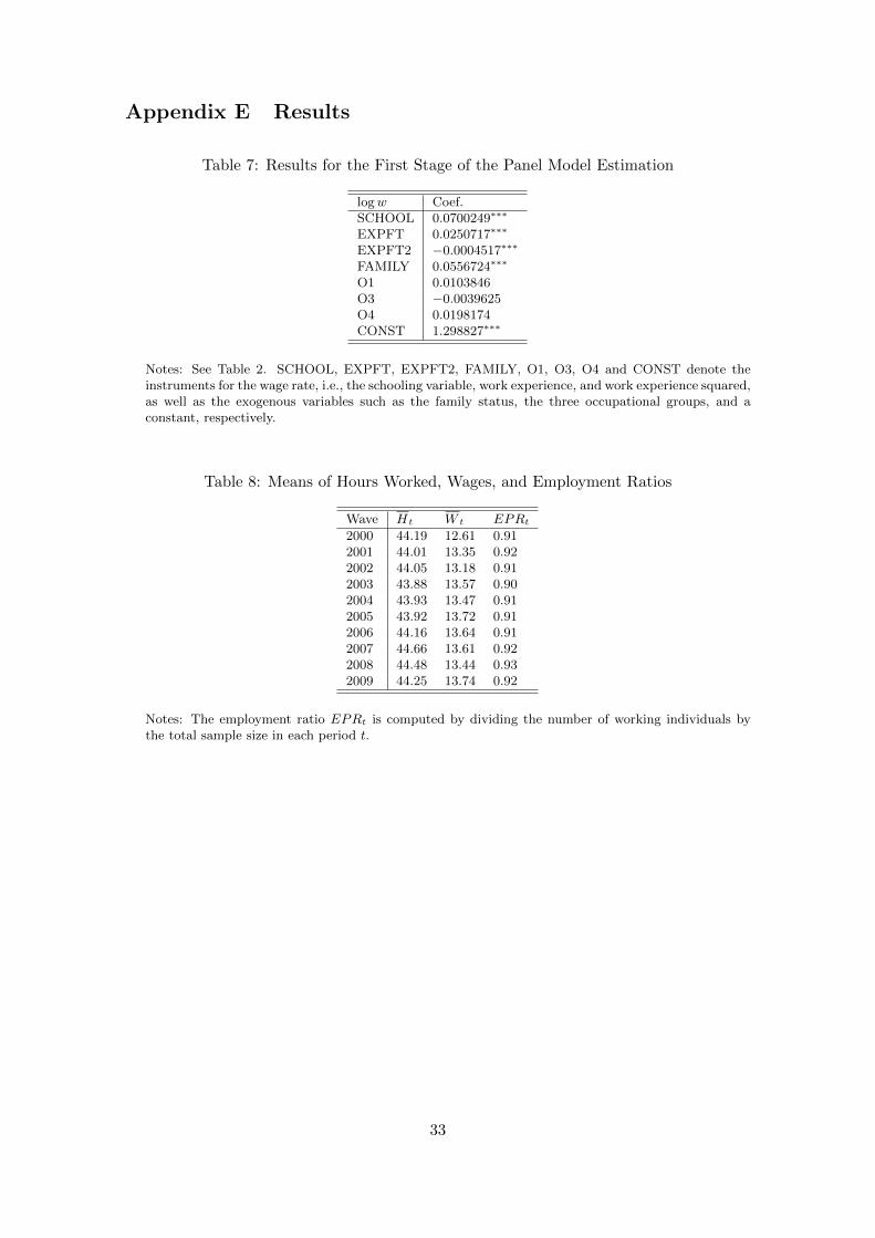
Appendix E Results

Table 7: Results for the First Stage of the Panel Model Estimation

logw Coef.SCHOOL 0.0700249∗∗∗

EXPFT 0.0250717∗∗∗

EXPFT2 −0.0004517∗∗∗

FAMILY 0.0556724∗∗∗

O1 0.0103846O3 −0.0039625O4 0.0198174CONST 1.298827∗∗∗

Notes: See Table 2. SCHOOL, EXPFT, EXPFT2, FAMILY, O1, O3, O4 and CONST denote theinstruments for the wage rate, i.e., the schooling variable, work experience, and work experience squared,as well as the exogenous variables such as the family status, the three occupational groups, and aconstant, respectively.

Table 8: Means of Hours Worked, Wages, and Employment Ratios

Wave Ht W t EPRt2000 44.19 12.61 0.912001 44.01 13.35 0.922002 44.05 13.18 0.912003 43.88 13.57 0.902004 43.93 13.47 0.912005 43.92 13.72 0.912006 44.16 13.64 0.912007 44.66 13.61 0.922008 44.48 13.44 0.932009 44.25 13.74 0.92

Notes: The employment ratio EPRt is computed by dividing the number of working individuals bythe total sample size in each period t.

33

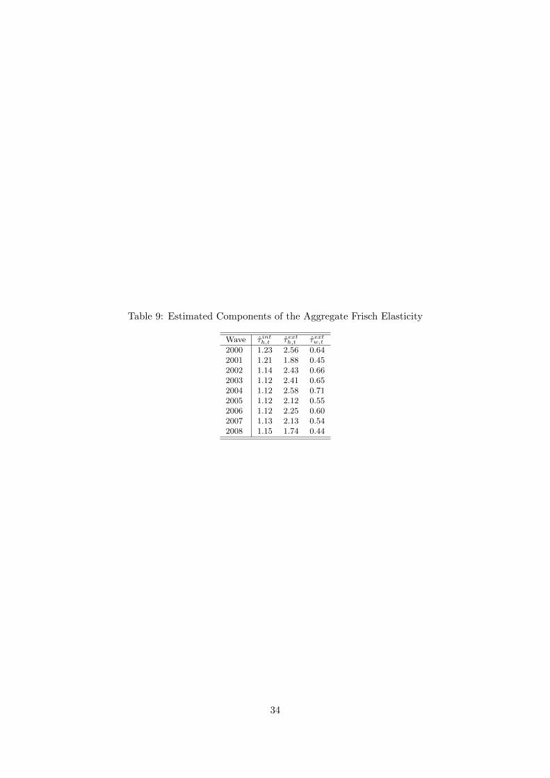
Table 9: Estimated Components of the Aggregate Frisch Elasticity

Wave τ inth,t τexth,t τextw,t

2000 1.23 2.56 0.642001 1.21 1.88 0.452002 1.14 2.43 0.662003 1.12 2.41 0.652004 1.12 2.58 0.712005 1.12 2.12 0.552006 1.12 2.25 0.602007 1.13 2.13 0.542008 1.15 1.74 0.44

34