Aggregation and the PPP Puzzle in a Sticky Price Model∗

(In progress; comments welcome)

Carlos CarvalhoFederal Reserve Bank of New York

Fernanda NechioPrinceton University

April, 2008

Abstract

We study the purchasing power parity (PPP) puzzle in a multi-sector, two country stickyprice model. Across sectors, firms differ in the extent of price stickiness, in accordance withrecent microeconomic evidence on price setting in various countries. Combined with local cur-rency pricing, this leads sectoral real exchange rates to have heterogeneous dynamics. We showanalytically that in such a heterogeneous economy deviations of the real exchange rate from PPPare more volatile and persistent than in a counterfactual one-sector world economy that features

the same average frequency of price changes, and is otherwise identical to the multi-sector worldeconomy. When calibrated to match the recent microeconomic evidence on the frequency ofprice changes, the model produces a half-life of deviations from PPP of 45 months. In contrast,the half-life of such deviations in the counterfactual one-sector economy is only slightly aboveone year. We provide a decomposition of this difference in persistence and find that over 90%of the gap is due to the fact that the counterfactual one-sector model is misspecified. An aggre-gation effect that arises in the heterogeneous economy accounts for the remaining fraction. Asa by-product, our results help clarify the “PPP Strikes Back debate” (Imbs et al. 2005a,b andChen and Engel 2005).

JEL classification codes: F3, F41, E0Keywords: heterogeneity, aggregation, price stickiness, real exchange rates, PPP puzzle

∗We thank seminar participants at the Federal Reserve Bank of New York and Princeton University for helpfulcomments. We are also grateful to Gianluca Benigno, Gauti Eggertsson, Pierre-Olivier Gourinchas, Jean Imbs, PaoloPesenti, Ricardo Reis, Hélène Rey, Chris Sims, and Thomas Wu for comments and suggestions. The views expressedin this paper are those of the authors and do not necessarily reflect the position of the Federal Reserve Bank of NewYork or the Federal Reserve System. E-mails: carlos.carvalho@ny.frb.org, fnechio@princeton.edu.

1

1 Introduction

Purchasing power parity (PPP) states that, once converted to the same currency, price levels across

countries should be equal. As a result, the real exchange rate between any two countries - the ratio

of their price levels in a common currency - should be constant and equal to unity. A more flexible

version of PPP postulates that real exchange rates should be constant, but not necessarily equal to

one. In contrast with the tight predictions of either version of PPP, in the data real exchange rates

display large and long-lived fluctuations around their average levels. Rogoff’s (1996) survey of the

empirical literature on the subject reports a “consensus view” that places estimates of the half-life

of deviations from PPP in the range of 3 to 5 years. While he suggests that the high volatility of the

real exchange rate could be explained by a model with monetary shocks and nominal rigidities, so

far models of this type with plausible nominal frictions have failed to produce the large persistence

found in the data; hence, the puzzle.

In this paper, we study the PPP puzzle in a multi-sector, two country, sticky price model. We

depart from the existing literature by introducing heterogeneity in the frequency of price changes

across sectors, in accordance with recent microeconomic evidence on price setting for various coun-

tries (e.g. Bils and Klenow 2004; Dhyne et al. 2006 for the Euro area). Combined with local

currency pricing, these differences in the extent of price stickiness lead sectoral real exchange rates

to have heterogeneous dynamics, which are also evident in the data (Imbs et al. 2005a).

We isolate the role of heterogeneity by comparing the dynamic behavior of the aggregate real

exchange rate in such a multi-sector economy with the behavior of the real exchange rate in an

otherwise identical one-sector world economy with the same average frequency of price changes. We

refer to this counterfactual economy as the misspecified one-sector world economy. We show that, in

response to nominal shocks, the aggregate real exchange rate in the heterogeneous economy is more

volatile and persistent than in the misspecified one-sector world economy, and that the difference

can be arbitrarily large.

We then investigate whether quantitatively our multi-sector model can solve the PPP puzzle, i.e.

produce highly volatile and persistent real exchange rates in response to monetary disturbances,

under a plausible calibration. In particular, to discipline our analysis we use a cross-sectional

distribution of the frequency of price changes that matches the recent microeconomic evidence

for the U.S. economy. We ask the same question in the misspecified one-sector world economy.

Our multi-sector model produces a half-life of deviations from PPP of 45 months, well within the

consensus view of 3 to 5 years. In contrast, such deviations in the one-sector world economy are

short-lived, with a half-life only slightly above one year. The volatility of the real exchange rate is

also much higher in the heterogeneous economy (by a factor that ranges from 2.5 to more than 5,

2

depending on the specification of the model).

The explanation for our results is that the counterfactual one-sector world economy is largely

misspecified with respect to the multi-sector model. As a result of cross-sectional aggregation

of sectoral exchange rates with heterogeneous dynamics, the aggregate real exchange rate in the

multi-sector economy displays much richer dynamics than the real exchange rate in the misspecified

one-sector model. As our analytical results show, the volatility and persistence of real exchange

rates are convex functions of the frequency of price adjustments, which leads the misspecified

one-sector model to understate both quantities relative to the underlying heterogeneous economy.

We start by presenting our multi-sector general equilibrium model in Section 2. It has two

countries trading intermediate goods produced by monopolistically competitive firms, which are

divided into sectors that differ in the frequency of price changes. Firms can price-discriminate

across the two countries, and set prices in the currency of the market in which the good is sold.

Consumers supply labor to these intermediate firms and consume the non-traded final good, which

is produced by competitive firms that bundle the intermediate goods from the two countries.

Using common assumptions about preferences and nominal shocks, Section 3 presents analytical

results that show that the volatility and persistence of the aggregate real exchange rate in the multi-

sector economy are larger than in the misspecified one-sector model. It provides a decomposition

of such difference in persistence into two terms: an aggregation effect - defined as the difference

between the persistence of the aggregate real exchange rate of the heterogeneous economy and the

(weighted) average persistence of sectoral exchange rates; and a misspecification effect - defined as

the difference between the former weighted average and the persistence of the real exchange rate

in the misspecified one-sector world economy. This decomposition clarifies the roles of aggregation

and misspecification in accounting for the difference in real exchange rate persistence across the

two world economies.

Section 4 presents the calibrated model using the cross-sectional distribution of the frequency

of price changes from Nakamura and Steinsson (2007). It shows that in response to monetary

shocks our multi-sector model generates much higher volatility and persistence than the misspec-

ified one-sector model. The misspecification effect accounts for well over 90% of this difference in

persistence, whereas the aggregation effect only explains the residual difference. We also present

several robustness exercises, and find that our results can survive important departures from the

baseline specification.

Finally, in Section 5 we use our structural model to revisit the discussion on the “aggregation

bias” and the PPP puzzle - the so called “PPP Strikes Back debate” (Imbs et al., 2005a,b and

Chen and Engel, 2005). Using the same data as in Imbs et al. (2005a), and our structural model as

3

a source of identifying restrictions, we estimate and decompose the total effect of heterogeneity on

persistence into the aggregation and misspecification effects. While the former only uses estimates

of persistence of real exchange rates for which we have data, the latter requires an estimate of

the persistence of the real exchange rate in the counterfactual one-sector economy. We show that,

under some conditions, this can be obtained by applying Mean Group estimators for panel datasets

with heterogeneous dynamics (Pesaran and Smith 1995).

In similarity with the results of the calibrated model, in the data we estimate a half-life of 46

months for aggregate real exchange rates, and 10 months for the counterfactual real exchange rate

process. As in the calibrated model, around 90% of the difference is explained by the misspecifica-

tion effect. In contrast, the aggregation effect only accounts for the small remaining fraction, given

that the average half-life of the underlying sector-country real exchange rates is very close to the

aggregate, at 43 months. We close Section 5 with a discussion of how our results help clarify the

“PPP Strikes Back debate.”

We conclude that our multi-sector sticky price model can solve the PPP puzzle. Thus, the

empirical properties of deviations from PPP only warrant the “puzzle” adjective if seen under the

lens of the misspecified one-sector model of the world economy. However, our findings still leave

open a series of important questions. These include the role of monetary policy, the nature of

shocks hitting the economy, and the stability of our findings across different policy regimes. We

conclude in Section 6 with a discussion of some of these issues.

Our paper is naturally related to the growing literature that focuses on the aggregate implica-

tions of heterogeneity in price setting.1 It contributes to the body of work that uses dynamic sticky

price models to study the persistence of real exchange rates, such as Bergin and Feenstra (2001),

Chari et al. (2002), Benigno (2004), and Steinsson (2008). There is also a connection between the

results from our multi-sector model, and the findings of the literature on cross-sectional aggrega-

tion of time-series processes (e.g. Granger and Morris 1976; Granger 1980; Zaffaroni 2004). Our

focus on economic implications as opposed to purely statistical aspects of aggregation also links

our work with Abadir and Talmain (2002). A specific version of our model is close to Kehoe and

Midrigan (2007), who analyze cross-sectional implications for sectoral real exchange rates. Finally,

our paper shares with Ghironi and Melitz (2005) and Atkeson and Burstein (2008) the themes of

heterogeneity and real exchange rate dynamics. However, while we focus on the PPP puzzle in a

sticky price model, they emphasize productivity shocks in flexible price models.

1Carvalho and Schwartzman (2008) provide detailed references.

4

2 The model

The world economy consists of two symmetric countries, Home and Foreign. In each country,

identical infinitely lived consumers supply labor to intermediate firms that they own, invest in

a complete set of state-contingent assets, and consume a non-traded final good. The latter is

produced by competitive firms that bundle varieties of intermediate goods produced in the two

countries. The monopolistically competitive intermediate firms that produce these varieties are

divided into sectors that differ in their frequency of price changes, and adjust prices as in Calvo

(1983). Labor is the variable input in the production of intermediate goods, which are the only

goods that are traded. Intermediate producers can price-discriminate across countries, and set

prices in local currency.

The Home representative consumer maximizes:

E0

∞Xt=0

βt

ÃC1−σt − 11− σ

− N1+γt

1 + γ

!,

subject to the flow budget constraint:

PtCt +Et [Θt,t+1Bt+1] ≤ PtWtNt +Bt + Tt,

where Et is the familiar time-t expectations operator, Ct is consumption of the final good, Nt is

labor, Pt is the price of the final good, Wt is the real wage, and Tt stands for profits received from

Home intermediate firms. Bt+1 stands for the state contingent value of the portfolio of financial

securities held by the consumer at the beginning of t+1. Complete markets allow agents to choose

the value of Bt+1 for each possible state of the world at all times, and a no-arbitrage condition

requires the existence of a nominal stochastic discount factor Θt,t+1 that prices in period t any

financial asset portfolio with value Bt+1 at the beginning of period t + 1. To avoid cluttering

the notation we omit explicit reference to the different states of nature. Finally, σ−1 denotes the

intertemporal elasticity of substitution and γ−1 is the Frisch elasticity of labor supply.

To rule out “Ponzi Schemes,” agents’ financial wealth must be, at all times and states, large

enough to avoid default:

Bt ≥ −∞Xs=0

Et [Θt,t+s (Pt+sWt+sNt+s + Tt+s)] ≥ −∞,

where Θt,t = 1, and Θt,t+s ≡Qt+s

r=t+1Θr−1,r for s > 0.

5

The first order conditions for the consumer’s problem are:

C−σt

C−σt+s

=βs

Θt,t+s

PtPt+s

, (1)

Nγt =WtC

−σt ,

where (1) holds for each future state of nature. The solution must also satisfy a transversality

condition:

lims→∞Et [Θt,t+sBt+s] = 0.

The Foreign consumer solves an analogous problem. She maximizes:

E0

∞Xt=0

βt

ÃC∗1−σt − 11− σ

− N∗1+γt

1 + γ

!,

subject to the flow budget constraint:

P ∗t C∗t +Et

∙Θ∗t,t+1

B∗t+1Et

¸≤ P ∗t W

∗t N

∗t +

B∗tEt + T ∗t , (2)

where a “∗” superscript denotes the Foreign counterpart of the corresponding Home variable, andEt is the nominal exchange rate, defined here as the price of the Foreign currency in terms of theHome currency. Et is thus quoted in units of Home currency per unit of the Foreign currency.Without loss of generality and for simplicity, we assume that the complete set of state-contingent

assets are denominated in the Home currency. As a result, in the budget constraint (2) B∗t appears

divided by the nominal exchange rate, to convert the value of the portfolio into Foreign currency.

The optimality conditions are:

C∗−σt

C∗−σt+s

=βs

Θ∗t,t+s

EtP ∗tEt+sP ∗t+s

, (3)

N∗γt =W ∗

t C∗−σt ,

where, again, (3) holds for each future state of nature, and a transversality condition:

lims→∞Et

£Θ∗t,t+sB

∗t+s

¤= 0.

The stochastic discount factor has to be the same for both countries, since assets are freely

traded and there are no arbitrage opportunities. Letting Qt ≡ Et P∗tPtdenote the real exchange rate,

6

from equations (1) and (3) this implies:

Qt+s = QtC−σt

C−σt+s

C∗−σt+s

C∗−σt

. (4)

Iterating equation (4) backwards and assuming Q0C−σ0C∗−σ0

= 1, yields:

Qt =C∗−σt

C−σt

.

The Home final good is produced by a representative competitive firm that bundles varieties of

intermediate goods from both countries. Each variety is produced by a monopolistically competitive

firm. Intermediate firms are divided into sectors indexed by k ∈ {1, ...,K}, each featuring acontinuum of firms. To highlight the role of heterogeneity in price stickiness, across sectors these

intermediate firms only differ in their pricing practices, as we detail below. Overall, firms are

indexed by the country where they produce, by their sector, and are further indexed by j ∈ [0, 1].The distribution of firms across sectors is given by sectoral weights fk > 0, with

PKk=1 fk = 1.

The technology employed to produce the final good is given by:

Yt =

µXK

k=1f1η

k Yη−1η

k,t

¶ ηη−1

, (5)

Yk,t =

µω1ρY

ρ−1ρ

H,k,t + (1− ω)1ρ Y

ρ−1ρ

F,k,t

¶ ρρ−1

, (6)

YH,k,t =

µfθ−1θ

k

Z 1

0Y

θ−1θ

H,k,j,tdj

¶ θθ−1

, (7)

YF,k,t =

µfθ−1θ

k

Z 1

0Y

θ−1θ

F,k,j,tdj

¶ θθ−1

, (8)

where Yt denotes the Home final good, Yk,t is the aggregation of the Home and Foreign intermediate

goods produced by sector k to be sold in Home, YH,k,t and YF,k,t are the aggregation of intermediate

varieties produced by firms in sector k in Home and Foreign, respectively, to be sold in Home, and

YH,k,j,t and YF,k,j,t are the varieties produced by firm j in sector k in Home and Foreign to be sold

in Home. Finally, η ≥ 0 is the elasticity of substitution across sectors, ρ ≥ 0 is the elasticity ofsubstitution between Home and Foreign goods, θ > 1 is the elasticity of substitution within sectors,

and ω ∈ [0, 1] is the steady-state share of domestic inputs.The maximization problem of a representative Home final good producing firm is:

max PtYt −µXK

k=1fk

Z 1

0(PH,k,j,tYH,k,j,t + PF,k,j,tYF,k,j,t) dj

¶s.t. (5)-(8).

7

The first order conditions, for j ∈ [0, 1] and k = 1, ...,K, are given by:

YH,k,j,t = ω

µPH,k,j,t

PH,k,t

¶−θ µPH,k,t

Pk,t

¶−ρµPk,tPt

¶−ηYt, (9)

YF,k,j,t = (1− ω)

µPF,k,j,tPF,k,t

¶−θ µPF,k,tPk,t

¶−ρµPk,tPt

¶−ηYt. (10)

The underlying price indices are:

Pt =

µXK

k=1fkP

1−ηk,t

¶ 11−η

, (11)

Pk,t =³ωP 1−ρH,k,t + (1− ω)P 1−ρF,k,t

´ 11−ρ

, (12)

PH,k,t =

µZ 1

0P 1−θH,k,j,tdj

¶ 11−θ

, (13)

PF,k,t =

µZ 1

0P 1−θF,k,j,tdj

¶ 11−θ

, (14)

where Pt is the price of the Home final good, Pk,t is the price index of sector k intermediate goods

sold in Home, PH,k,t is the price index for sector k Home-produced intermediate goods sold in

Home, and PH,k,j,t is the price charged in the Home market by Home firm j from sector k. PF,k,t is

the price index for sector k Foreign-produced intermediate goods sold in Home, and PF,k,j,t is the

price charged in the Home market by Foreign firm j from sector k. Both PH,k,j,t and PF,k,j,t are

set in the Home currency.

With an analogous maximization problem, the Foreign final firm chooses its demands for inter-

mediate inputs from Foreign (Y ∗F,k,j,t) and Home (Y∗H,k,j,t) producers:

Y ∗F,k,j,t = ω

ÃP ∗F,k,j,tP ∗F,k,t

!−θÃP ∗F,k,tP ∗F,t

!−ρµP ∗k,tP ∗t

¶−ηY ∗t , (15)

Y ∗H,k,j,t = (1− ω)

ÃP ∗H,k,j,t

P ∗H,k,t

!−θÃP ∗H,k,t

P ∗k,t

!−ρµP ∗k,tP ∗t

¶−ηY ∗t . (16)

The Foreign price indices are analogous to the Home ones (equations (11)-(14)):

P ∗t =

µXK

k=1fkP

∗1−ηk,t

¶ 11−η

, (17)

P ∗k,t =³ωP ∗1−ρF,k,t + (1− ω)P ∗1−ρH,k,t

´ 11−ρ

, (18)

8

P ∗H,k,t =

µZ 1

0P ∗1−θH,k,j,tdj

¶ 11−θ

, (19)

P ∗F,k,t =

µZ 1

0P ∗1−θF,k,j,tdj

¶ 11−θ

, (20)

where P ∗t is the price of the Foreign final good, P ∗k,t is the price index of sector k intermediate

goods sold in Foreign, P ∗F,k,t is the price index for sector k Foreign-produced intermediate goods

sold in Foreign, and P ∗F,k,j,t is the price charged in the Foreign market by Foreign firm j from sector

k. P ∗H,k,t is the price index for sector k Home-produced intermediate goods sold in Foreign, and

P ∗H,k,j,t is the price charged in the Foreign market by Home firm j from sector k. Both P ∗F,k,j,t and

P ∗H,k,j,t are set in the Foreign currency.

For ease of reference, we refer to PH,k,t, PF,k,t, P∗H,k,t, P

∗F,k,t as country-sector price indices, and

to Pk,t, P ∗k,t as sectoral price indices. We can then define the sectoral real exchange rate for sector

k as the ratio of sectoral price indices in a common currency:

Qk,t ≡ EtP ∗k,tPk,t

.

Intermediate firms set prices as in Calvo (1983). The frequency of price changes varies across

sectors, and is the only source of (ex-ante) heterogeneity. Thus, sectors in the model are naturally

identified with their frequency of price changes. In each period, each firm j in sector k changes its

price independently with probability αk. To keep track of the sectors, we order them in terms of

increasing price stickiness, so that α1 > ... > αK .

Each time Home firm j from sector k adjusts, it chooses prices XH,k,j,t, X∗H,k,j,t to be charged

in the Home and Foreign markets, respectively, with each price being set in the corresponding local

currency. Thus, its maximization problem is:

max Et

∞Xs=0

Θt,t+s (1− αk)s ¡XH,k,j,tYH,k,j,t+s + Et+sX∗

H,k,j,tY∗H,k,j,t+s − Pt+sWt+sNk,j,t+s

¢

s.t. (9), (16),

YH,k,j,t + Y ∗H,k,j,t = Nχk,j,t, (21)

where Nk,j,t is the amount of labor it employs, and χ determines returns to labor.

The first order conditions are:

XH,k,j,t =θ

θ − 1EtP∞

s=0Θt,t+s (1− αk)s ΛH,k,t+s

³χNχ−1

k,j,t+s

´−1Pt+sWt+s

EtP∞

s=0Θt,t+s (1− αk)s ΛH,k,t+s

,

9

X∗H,k,j,t =

θ

θ − 1EtP∞

s=0Θt,t+s (1− αk)s Λ∗H,k,t+s

³χNχ−1

k,j,t+s

´−1Pt+sWt+s

EtP∞

s=0Θt,t+s (1− αk)s Et+sΛ∗H,k,t+s

,

where:

ΛH,k,t = ω

µ1

PH,k,t

¶−θ µPH,k,t

Pk,t

¶−ρµPk,tPt

¶−ηYt,

Λ∗H,k,t = (1− ω)

Ã1

P ∗H,k,t

!−θÃP ∗H,k,t

P ∗k,t

!−ρµP ∗k,tP ∗t

¶−ηY ∗t .

An analogous maximization problem for the Foreign firms yields:

X∗F,k,j,t =

θ

θ − 1EtP∞

s=0Θ∗t,t+s (1− αk)

s Λ∗F,k,t+s³χN∗χ−1

k,j,t+s

´−1P ∗t+sW ∗

t+s

EtP∞

s=0Θ∗t,t+s (1− αk)

s Λ∗F,k,t+s,

XF,k,j,t =θ

θ − 1EtP∞

s=0Θ∗t,t+s (1− αk)

s ΛF,k,t+s

³χN∗χ−1

k,j,t+s

´−1P ∗t+sW ∗

t+s

EtP∞

s=0Θ∗t,t+s (1− αk)

s E−1t+sΛF,k,t+s,

where:

Λ∗F,k,t = ω

Ã1

P ∗F,k,t

!−θÃP ∗F,k,tP ∗k,t

!−ρµP ∗k,tP ∗t

¶−ηY ∗t ,

ΛF,k,t = (1− ω)

µ1

PF,k,t

¶−θ µPF,k,tPk,t

¶−ρµPF,tPt

¶−ηYt.

We focus on a symmetric equilibrium in which, conditional on time t information, the joint

distribution of future variables that matter for price setting is the same for all firms in sector k in a

given country that change prices in period t. Therefore, they make the same pricing decisions, and

choose prices that we denote by XH,k,t, X∗H,k,t, and XF,k,t, X

∗F,k,t. The country-sector price indices

can thus be written as:

PH,k,t =³αkX

1−θH,k,t + (1− αk)P

1−θH,k,t−1

´ 11−θ

,

P ∗H,k,t =³αkX

∗1−θH,k,t + (1− αk)P

∗1−θH,k,t−1

´ 11−θ

,

and likewise for PF,k,t and P ∗F,k,t.

Finally, the model is closed by a monetary policy specification that ensures existence and unique-

ness of the rational expectations equilibrium. We consider different specifications in subsequent

sections. Equilibrium is characterized by the optimality conditions of the consumers’ utility maxi-

mization problem and of every firm’s profit maximization problem, and by market clearing in assets,

10

goods and labor markets.

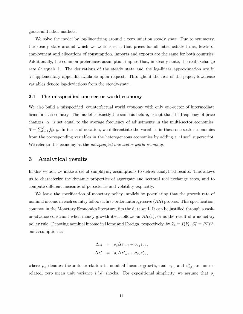
We solve the model by log-linearizing around a zero inflation steady state. Due to symmetry,

the steady state around which we work is such that prices for all intermediate firms, levels of

employment and allocations of consumption, imports and exports are the same for both countries.

Additionally, the common preferences assumption implies that, in steady state, the real exchange

rate Q equals 1. The derivations of the steady state and the log-linear approximation are in

a supplementary appendix available upon request. Throughout the rest of the paper, lowercase

variables denote log-deviations from the steady-state.

2.1 The misspecified one-sector world economy

We also build a misspecified, counterfactual world economy with only one-sector of intermediate

firms in each country. The model is exactly the same as before, except that the frequency of price

changes, α, is set equal to the average frequency of adjustments in the multi-sector economies:

α =PK

k=1 fkαk. In terms of notation, we differentiate the variables in these one-sector economies

from the corresponding variables in the heterogeneous economies by adding a “1 sec” superscript.

We refer to this economy as the misspecified one-sector world economy.

3 Analytical results

In this section we make a set of simplifying assumptions to deliver analytical results. This allows

us to characterize the dynamic properties of aggregate and sectoral real exchange rates, and to

compute different measures of persistence and volatility explicitly.

We leave the specification of monetary policy implicit by postulating that the growth rate of

nominal income in each country follows a first-order autoregressive (AR) process. This specification,

common in the Monetary Economics literature, fits the data well. It can be justified through a cash-

in-advance constraint when money growth itself follows an AR (1), or as the result of a monetary

policy rule. Denoting nominal income in Home and Foreign, respectively, by Zt ≡ PtYt, Z∗t ≡ P ∗t Y ∗t ,

our assumption is:

∆zt = ρz∆zt−1 + σεzεz,t,

∆z∗t = ρz∆z∗t−1 + σεzε

∗z,t,

where ρz denotes the autocorrelation in nominal income growth, and εz,t and ε∗z,t are uncor-

related, zero mean unit variance i.i.d. shocks. For expositional simplicity, we assume that ρz

11

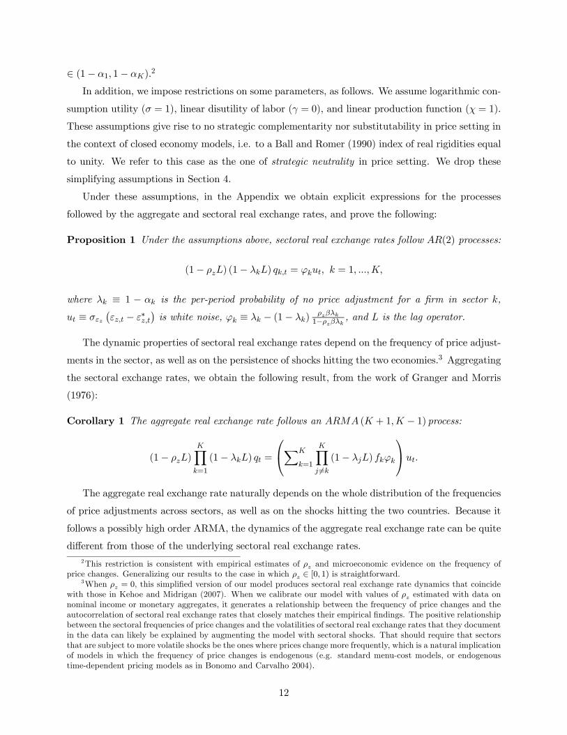
∈ (1− α1, 1− αK).2

In addition, we impose restrictions on some parameters, as follows. We assume logarithmic con-

sumption utility (σ = 1), linear disutility of labor (γ = 0), and linear production function (χ = 1).

These assumptions give rise to no strategic complementarity nor substitutability in price setting in

the context of closed economy models, i.e. to a Ball and Romer (1990) index of real rigidities equal

to unity. We refer to this case as the one of strategic neutrality in price setting. We drop these

simplifying assumptions in Section 4.

Under these assumptions, in the Appendix we obtain explicit expressions for the processes

followed by the aggregate and sectoral real exchange rates, and prove the following:

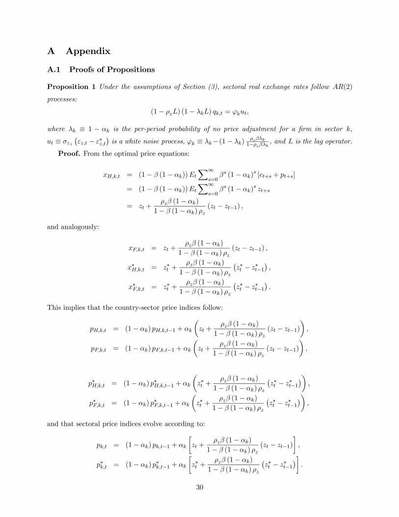
Proposition 1 Under the assumptions above, sectoral real exchange rates follow AR(2) processes:

(1− ρzL) (1− λkL) qk,t = ϕkut, k = 1, ...,K,

where λk ≡ 1 − αk is the per-period probability of no price adjustment for a firm in sector k,

ut ≡ σεz¡εz,t − ε∗z,t

¢is white noise, ϕk ≡ λk − (1− λk)

ρzβλk1−ρzβλk , and L is the lag operator.

The dynamic properties of sectoral real exchange rates depend on the frequency of price adjust-

ments in the sector, as well as on the persistence of shocks hitting the two economies.3 Aggregating

the sectoral exchange rates, we obtain the following result, from the work of Granger and Morris

(1976):

Corollary 1 The aggregate real exchange rate follows an ARMA (K + 1,K − 1) process:

(1− ρzL)KYk=1

(1− λkL) qt =

⎛⎝XK

k=1

KYj 6=k

(1− λjL) fkϕk

⎞⎠ut.

The aggregate real exchange rate naturally depends on the whole distribution of the frequencies

of price adjustments across sectors, as well as on the shocks hitting the two countries. Because it

follows a possibly high order ARMA, the dynamics of the aggregate real exchange rate can be quite

different from those of the underlying sectoral real exchange rates.2This restriction is consistent with empirical estimates of ρz and microeconomic evidence on the frequency of

price changes. Generalizing our results to the case in which ρz ∈ [0, 1) is straightforward.3When ρz = 0, this simplified version of our model produces sectoral real exchange rate dynamics that coincide

with those in Kehoe and Midrigan (2007). When we calibrate our model with values of ρz estimated with data onnominal income or monetary aggregates, it generates a relationship between the frequency of price changes and theautocorrelation of sectoral real exchange rates that closely matches their empirical findings. The positive relationshipbetween the sectoral frequencies of price changes and the volatilities of sectoral real exchange rates that they documentin the data can likely be explained by augmenting the model with sectoral shocks. That should require that sectorsthat are subject to more volatile shocks be the ones where prices change more frequently, which is a natural implicationof models in which the frequency of price changes is endogenous (e.g. standard menu-cost models, or endogenoustime-dependent pricing models as in Bonomo and Carvalho 2004).

12

Finally, the real exchange rate in the misspecified one-sector world economy can be obtained as

a degenerate case in which all firms belong to a single sector, with frequency of price adjustments

equal to the average frequency of the heterogeneous economy:

Corollary 2 The real exchange rate of the misspecified one-sector world economy follows an AR (2)

process:

(1− ρzL)¡1− λL

¢q1 sect = ϕut,

where λ ≡PKk=1 fkλk and ϕ ≡ λ− ¡1− λ

¢ ρzβλ

1−ρzβλ.

3.1 Persistence

We are interested in analyzing the persistence of deviations of the real exchange rate from PPP.

In this subsection we focus on measures of persistence used in the literature for which we can

obtain analytical results. In particular, we focus on the cumulative impulse response, the largest

autoregressive root, and the sum of autoregressive coefficients. The cumulative impulse response

(CIR) is defined as follows. Let IRFt (q) , t = 0, 1, ... denote the impulse response function (to aunit impulse) of the qt process. Then, CIR (q) ≡

P∞t=0 IRFt (q). The largest autoregressive root

(LAR) for a process qt with representation eA (L) qt = eB (L)ut, LAR (q), is simply the largest rootof the eA (L) polynomial. Finally, the sum of autoregressive coefficients (SAC) of such a process isSAC (q) ≡ 1− eA (1). In Section 4 we use calibrated versions of the model to assess the quantitativeimportance of our analytical findings in terms of these and other measures of persistence, such as

the half-life.4

Let P denote one such measure of persistence. We prove the following:

Proposition 2 For the measures of persistence P = CIR,LAR,SAC:

P (q) > P ¡q1 sec¢ .Proposition 2 shows that a simple model with sectoral heterogeneity stemming solely from

differences in the frequency of price changes can generate an aggregate real exchange rate that is

more persistent than the real exchange rate in a one-sector version of the world economy with the

same average frequency of price changes.

As will become clear, the main determinant of this result is the fact that the counterfactual

one-sector model is largely misspecified under the multi-sector model. Corollary 1 shows that as4The literature focuses mainly on the half-life of estimated real exchange rate processes, and on the first auto-

correlation under the assumption of AR(1) specifications for the purpose of providing analytical results. However,the latter becomes less meaningful as one moves away from AR(1) specifications as we do in our model. Moreover,beyond the AR(1) case it is quite difficult to obtain analytical results for the half-life.

13

a result of cross-sectional aggregation of sectoral exchange rates with heterogeneous dynamics, the

aggregate real exchange rate in the multi-sector economy follows a much richer stochastic process

than the real exchange rate in the misspecified one-sector model. Moreover, the persistence of

real exchange rates under these commonly used measures is a convex function of the frequency of

price adjustments. Thus, the misspecified one-sector model understates the persistence of the real

exchange rate relative to the underlying heterogeneous economy.

Our next result will prove helpful in understanding the source of that difference in persistence.

For any measure of persistence P, we define the total heterogeneity effect under P to be the

difference between the persistence of the aggregate real exchange rate in the heterogeneous economy,

qt, and the persistence of the real exchange rate in the misspecified one-sector world economy, q1 sect :

total heterogeneity effect under P ≡ P (q)− P ¡q1 sec¢ .We can rewrite the total heterogeneity effect by adding and subtracting the weighted average of

the persistence of the sectoral exchange rates,PK

k=1 fkP (qk), to obtain the following decomposition:

total heterogeneity

effect under P =

µP (q)−

XK

k=1fkP (qk)

¶+

µXK

k=1fkP (qk)− P

¡q1 sec

¢¶. (22)

In (22), the first term in parentheses is what we refer to as the aggregation effect under P: thedifference between the “persistence of the average” and the “average of the persistences”:

aggregation effect under P ≡ P (q)−XK

k=1fkP (qk) . (23)

Since the aggregate real exchange rate is equal to the weighted average of the sectoral exchange

rates, the measure in (23) is indeed purely a result of aggregation.

The second term in the decomposition (22) is the difference between the weighted average of

the persistence of sectoral real exchange rates in the heterogeneous economy, and the persistence

of the real exchange rate in the misspecified one-sector world economy:

misspecification effect under P ≡XK

k=1fkP (qk)− P

¡q1 sec

¢. (24)

Our next result gives substance to the decomposition in (22), by showing that both the aggre-

gation and the misspecification effects are positive:

14

Proposition 3 For the measures of persistence P = CIR,LAR,SAC:

aggregation effect under P > 0,

misspecification effect under P ≥ 0.

In particular:5

CIR :aggregation effect > 0,

misspecification effect > 0;

LAR :aggregation effect > 0,

misspecification effect > 0;

SAC :aggregation effect > 0,

misspecification effect = 0.

For almost every case, both the aggregation and the misspecification effects are strictly positive.

The only exception is when persistence is measured through the sum of autoregressive coefficients,

in which case the misspecification effect is zero. This is a general result for measures of persistence

that are linear in the autoregressive coefficients - the sum of autoregressive coefficients is an example

- and is formalized below:

Lemma 1 For measures of persistence that are linear in the autoregressive coefficients:

XK

k=1fkP (qk) = P

¡q1 sec

¢,

so that the misspecification effect is zero.

Lemma 1 follows directly from the fact that in the AR (2) process followed by the real exchange

rate in the misspecified one-sector world economy, the autoregressive coefficient at each lag equals

the weighted average of the corresponding autoregressive coefficients of the sectoral exchange rates.

Thus, for the special case of linear measures of persistence, the misspecification effect is zero, and

the aggregation effect equals the total heterogeneity effect. We use this result in Section 5, when

we revisit the “PPP Strikes Back debate.”

3.2 Volatility

The other dimension of the PPP puzzle is the high volatility of the real exchange rate. Comparing

the real exchange rate in the misspecified one-sector world economy, and the sectoral real exchange

rates in the heterogeneous economy, the following result holds:5Below we omit the “under P” qualifier, since it is clear from the context.

15

Proposition 4 Let V (qk) denote the unconditional variance of the qk,t process. Then:XK

k=1fkV (qk) > V

¡q1 sec

¢.

Proposition 4 shows that the average volatility of sectoral real exchange rates in the multi-

sector world economy exceeds the volatility of the real exchange rate in the misspecified one-sector

model. However, this is not a comparison between the latter and the aggregate real exchange rate

in the multi-sector model. In the calibrated versions of the model analyzed in Section 4, we find

that the volatility of the aggregate real exchange rate also exceeds that of the real exchange rate

in the misspecified one-sector world economy.

3.3 A limiting result

This subsection shows that a “suitably heterogeneous” multi-sector world economy can generate an

aggregate real exchange rate that is arbitrarily more volatile and persistent than the real exchange

rate in the misspecified one-sector world economy.6 We consider the effects of progressively adding

more sectors, and assume that the frequency of price changes for each new sector is drawn from

(0, 1− δ) for arbitrarily small δ > 0, according to some distribution with density g (α|b), where αis the frequency of price changes and b is a parameter. For α ≈ 0 such density is assumed to beapproximately proportional to α−b, with b ∈ ¡12 , 1¢.7 The shape of this distribution away from zeroneed not be specified, and moreover it yields a strictly positive average frequency of price changes:

α =R 1−δ0 g (α|b)αdα > 0.

We prove the following:

Proposition 5 Under the assumptions above:

Vµ1

K

XK

k=1qk,t

¶−→K→∞

∞,

CIR

µ1

K

XK

k=1qk,t

¶−→K→∞

∞,

V ¡q1 sec¢ , CIR ¡q1 sec¢ <∞.

The results in Proposition 5 follow from the fact that, under suitable assumptions, the aggre-

gate real exchange rate converges to a non-stationary process. It inherits some features of unit-root6We build on the work of Granger (1980), Granger and Joyeux (1980), Zaffaroni (2004) and others.7Thus, we approximate a large number of potential new sectors by a continuum, and replace the general fk

distribution by this semi-parametric specification for g (α|b), based on Zaffaroni (2004). An example of a parametricdistribution that satisfies this restriction is a Beta distribution with suitably chosen support and parameters.

16

processes, such as infinite variance and persistence, due to the relatively high density of very persis-

tent sectoral real exchange rates embedded in the distributional assumption for the frequencies of

price changes. However, the process does not have a unit root, since none of the sectoral exchange

rates actually has one. Moreover, the limiting process remains mean reverting in the sense that its

impulse response function converges to zero as t −→ ∞.8 In contrast, the limiting process for thereal exchange rate in the misspecified one-sector world economy remains stationary, since α > 0

and as such, it has both finite variance and persistence.

In qualitative terms, Propositions 2-5 provide an affirmative answer to the question of whether

a model with heterogeneity in price stickiness can solve the PPP puzzle. However, to answer the

more relevant question of whether a version of the model calibrated to match the microeconomic

evidence on the frequency of price changes does in fact account for the puzzle we must go beyond

qualitative results. We turn to that question next.

4 Quantitative analysis

In this section we analyze the quantitative implications of calibrated versions of our model. We de-

scribe our calibration, starting with how we use the recent microeconomic evidence on price setting

to calibrate the cross-sectional distribution of price stickiness. We then present the quantitative

results for our baseline specification, and consider alternative configurations as robustness checks.

In particular, we consider the case in which monetary policy follows an interest rate rule subject

to persistent shocks, and allow for productivity shocks. We also consider the case of strategic

neutrality in price setting.

4.1 Calibration

4.1.1 Cross-sectional distribution of price stickiness

A series of recent papers have documented several features of price setting behavior in modern

industrial economies using disaggregated price data that underlies consumer price indices (e.g. Bils

and Klenow 2004, and Nakamura and Steinsson 2007 for the U.S. economy; Dhyne et al. 2006,

and references cited therein for the Euro area; Gagnon 2007 for Mexico). In turn, Gopinath and

Rigobon (2008) document price setting practices using disaggregated price data on U.S. imports

and exports.

In our model, whenever a firm changes its prices it sets one price for the domestic market and

another price for exports, and for simplicity we impose the same frequency of price adjustments

8Such properties characterize the so-called fractionally integrated processes. See, for example, Granger and Joyeux(1980).

17

in both cases.9 In addition, we also assume the same cross-sectional distribution of the frequency

of price changes in both countries. As a result, we must choose a single suitable distribution to

calibrate the model.

We analyze our model having in mind a two-country world economy with the U.S. and the rest

of the world. Since the domestic market is relatively more important for firms decisions (due to a

small import share), we favor a distribution for the frequency of price changes across sectors that

reflects mainly domestic rather than export pricing decisions. Due to our assumption of symmetric

countries, we also favor distributions that are representative of price setting behavior in different

developed economies. Finally, and perhaps most importantly, we want to relate our results to

the empirical PPP literature, which most often focuses on real exchange rates based on consumer

price indices (CPIs). As a result, we choose to use the statistics on the frequency of price changes

reported by Nakamura and Steinsson (2007).

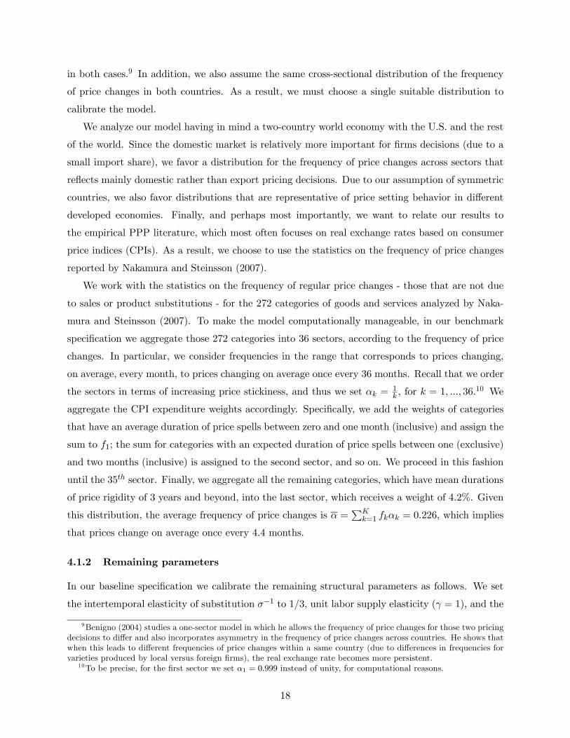
We work with the statistics on the frequency of regular price changes - those that are not due

to sales or product substitutions - for the 272 categories of goods and services analyzed by Naka-

mura and Steinsson (2007). To make the model computationally manageable, in our benchmark

specification we aggregate those 272 categories into 36 sectors, according to the frequency of price

changes. In particular, we consider frequencies in the range that corresponds to prices changing,

on average, every month, to prices changing on average once every 36 months. Recall that we order

the sectors in terms of increasing price stickiness, and thus we set αk = 1k , for k = 1, ..., 36.

10 We

aggregate the CPI expenditure weights accordingly. Specifically, we add the weights of categories

that have an average duration of price spells between zero and one month (inclusive) and assign the

sum to f1; the sum for categories with an expected duration of price spells between one (exclusive)

and two months (inclusive) is assigned to the second sector, and so on. We proceed in this fashion

until the 35th sector. Finally, we aggregate all the remaining categories, which have mean durations

of price rigidity of 3 years and beyond, into the last sector, which receives a weight of 4.2%. Given

this distribution, the average frequency of price changes is α =PK

k=1 fkαk = 0.226, which implies

that prices change on average once every 4.4 months.

4.1.2 Remaining parameters

In our baseline specification we calibrate the remaining structural parameters as follows. We set

the intertemporal elasticity of substitution σ−1 to 1/3, unit labor supply elasticity (γ = 1), and the

9Benigno (2004) studies a one-sector model in which he allows the frequency of price changes for those two pricingdecisions to differ and also incorporates asymmetry in the frequency of price changes across countries. He shows thatwhen this leads to different frequencies of price changes within a same country (due to differences in frequencies forvarieties produced by local versus foreign firms), the real exchange rate becomes more persistent.

10To be precise, for the first sector we set α1 = 0.999 instead of unity, for computational reasons.

18

usual extent of decreasing returns to labor (χ = 2/3). The consumer discount factor β implies a

time-discount rate of 2% per year.

For the final good technology parameters, we set the elasticity of substitution between varieties

of the same sector to θ = 10. We set the elasticity of substitution between Home and Foreign

goods to ρ = 1.5, and the share of domestic goods at ω = 0.9.11 The elasticity of substitution

between varieties of different sectors should be smaller than within sectors, and so we assume a

unit elasticity of substitution across sectors, η = 1 (i.e. the aggregator that converts sectoral into

final output is Cobb-Douglas).

Finally, to calibrate the process for nominal income, the literature usually relies on estimates

based on nominal GDP, or on monetary aggregates such as M1 or M2. With quarterly data,

estimates of ρz typically fall in the range of 0.4 to 0.7.12 This maps into a range of 0.74 − 0.89

at a monthly frequency, and so we set ρz = 0.8. The standard deviation of the shocks is set at

σεz = 0.58% (1% at a quarterly frequency), also in line with the same estimation results.

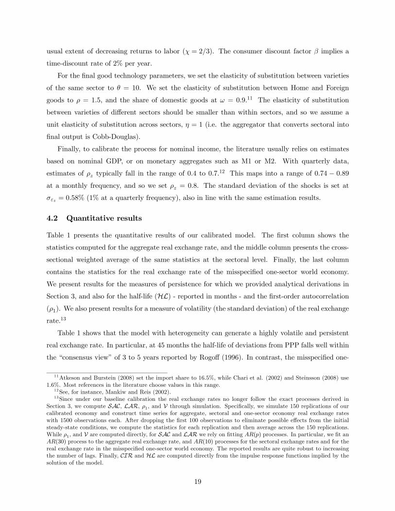
4.2 Quantitative results

Table 1 presents the quantitative results of our calibrated model. The first column shows the

statistics computed for the aggregate real exchange rate, and the middle column presents the cross-

sectional weighted average of the same statistics at the sectoral level. Finally, the last column

contains the statistics for the real exchange rate of the misspecified one-sector world economy.

We present results for the measures of persistence for which we provided analytical derivations in

Section 3, and also for the half-life (HL) - reported in months - and the first-order autocorrelation(ρ1). We also present results for a measure of volatility (the standard deviation) of the real exchange

rate.13

Table 1 shows that the model with heterogeneity can generate a highly volatile and persistent

real exchange rate. In particular, at 45 months the half-life of deviations from PPP falls well within

the “consensus view” of 3 to 5 years reported by Rogoff (1996). In contrast, the misspecified one-

11Atkeson and Burstein (2008) set the import share to 16.5%, while Chari et al. (2002) and Steinsson (2008) use1.6%. Most references in the literature choose values in this range.

12See, for instance, Mankiw and Reis (2002).13Since under our baseline calibration the real exchange rates no longer follow the exact processes derived in

Section 3, we compute SAC, LAR, ρ1, and V through simulation. Specifically, we simulate 150 replications of ourcalibrated economy and construct time series for aggregate, sectoral and one-sector economy real exchange rateswith 1500 observations each. After dropping the first 100 observations to eliminate possible effects from the initialsteady-state conditions, we compute the statistics for each replication and then average across the 150 replications.While ρ1, and V are computed directly, for SAC and LAR we rely on fitting AR(p) processes. In particular, we fit anAR(30) process to the aggregate real exchange rate, and AR(10) processes for the sectoral exchange rates and for thereal exchange rate in the misspecified one-sector world economy. The reported results are quite robust to increasingthe number of lags. Finally, CIR and HL are computed directly from the impulse response functions implied by thesolution of the model.

19

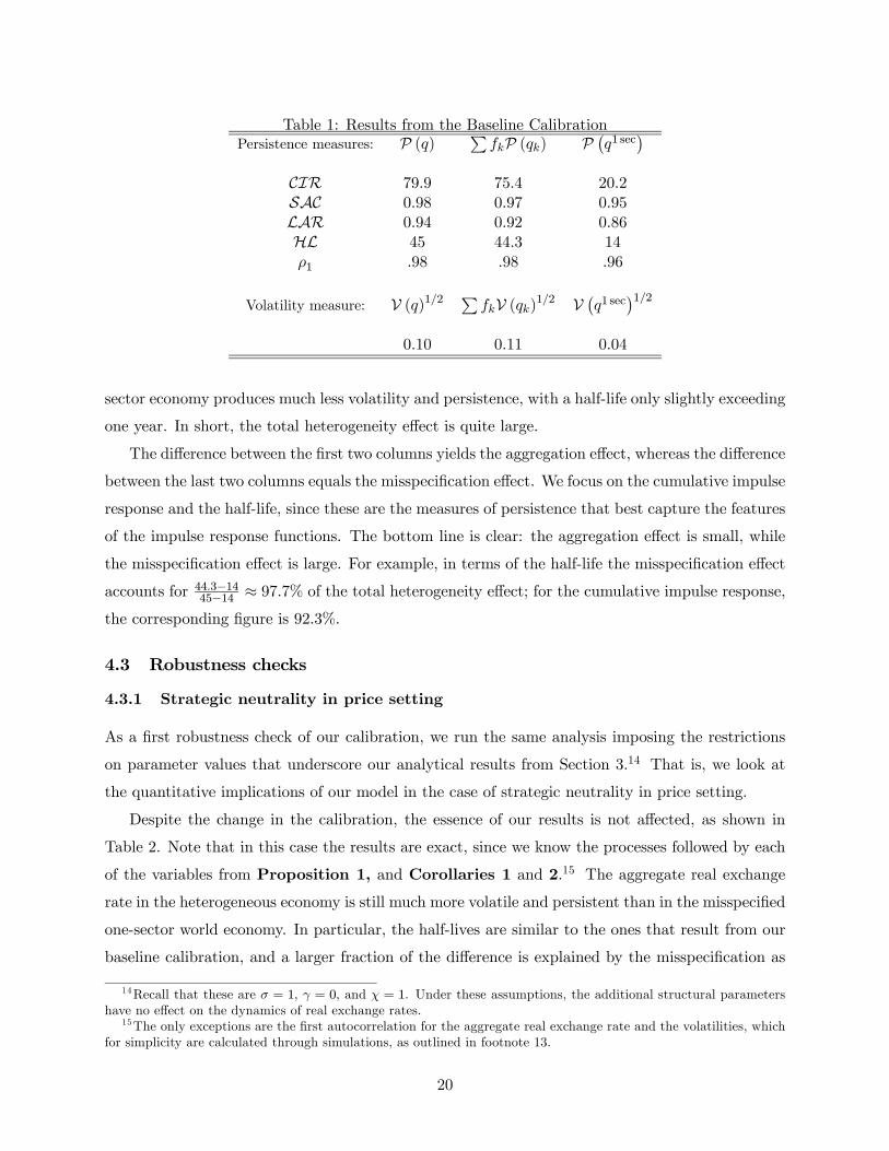
Table 1: Results from the Baseline CalibrationPersistence measures: P (q) P

fkP (qk) P ¡q1 sec¢CIR 79.9 75.4 20.2SAC 0.98 0.97 0.95LAR 0.94 0.92 0.86HL 45 44.3 14ρ1 .98 .98 .96

Volatility measure: V (q)1/2 PfkV (qk)1/2 V ¡q1 sec¢1/2

0.10 0.11 0.04

sector economy produces much less volatility and persistence, with a half-life only slightly exceeding

one year. In short, the total heterogeneity effect is quite large.

The difference between the first two columns yields the aggregation effect, whereas the difference

between the last two columns equals the misspecification effect. We focus on the cumulative impulse

response and the half-life, since these are the measures of persistence that best capture the features

of the impulse response functions. The bottom line is clear: the aggregation effect is small, while

the misspecification effect is large. For example, in terms of the half-life the misspecification effect

accounts for 44.3−1445−14 ≈ 97.7% of the total heterogeneity effect; for the cumulative impulse response,

the corresponding figure is 92.3%.

4.3 Robustness checks

4.3.1 Strategic neutrality in price setting

As a first robustness check of our calibration, we run the same analysis imposing the restrictions

on parameter values that underscore our analytical results from Section 3.14 That is, we look at

the quantitative implications of our model in the case of strategic neutrality in price setting.

Despite the change in the calibration, the essence of our results is not affected, as shown in

Table 2. Note that in this case the results are exact, since we know the processes followed by each

of the variables from Proposition 1, and Corollaries 1 and 2.15 The aggregate real exchange

rate in the heterogeneous economy is still much more volatile and persistent than in the misspecified

one-sector world economy. In particular, the half-lives are similar to the ones that result from our

baseline calibration, and a larger fraction of the difference is explained by the misspecification as

14Recall that these are σ = 1, γ = 0, and χ = 1. Under these assumptions, the additional structural parametershave no effect on the dynamics of real exchange rates.

15The only exceptions are the first autocorrelation for the aggregate real exchange rate and the volatilities, whichfor simplicity are calculated through simulations, as outlined in footnote 13.

20

opposed to the aggregation effect.16

Table 2: Results under Strategic Neutrality in Price SettingPersistence measures: P (q) P

fkP (qk) P ¡q1 sec¢CIR 87.3 65.2 22.2SAC ≈ 1 0.85 0.85LAR .97 0.89 0.8HL 47 34 15ρ1 0.99 0.96 .97

Volatility measure: V (q)1/2 PfkV (qk)1/2 V ¡q1 sec¢1/2

0.06 0.06 0.02

4.3.2 Different shocks

We consider a specification with an explicit description of monetary policy, and later also add

productivity shocks. We assume that in each country monetary policy is conducted according

to an interest rate rule. Motivated by the results obtained by Rudebusch (2002), we assume a

specification subject to persistent shocks, as follows:

It = β

µPtPt−1

¶φπµYtY nt

¶φY

eυt ,

where It is the short term nominal interest rate in Home, Y nt is the natural output, defined as

output if all prices were flexible, φπ and φY are the parameters associated with Taylor interest rate

rules, and υt is a persistent shock with process υt = ρυυt−1 + σευευ,t, where ευ,t is a zero mean,

unit variance i.i.d. shock, and ρυ ∈ [0, 1). The policy rule in Foreign is analogous, and we assumethat the shocks are uncorrelated across countries. We set φπ = 1.5, φy = .5/12, and ρυ = 0.965.

17

The remaining parameter values are unchanged from the baseline specification.

The results are in Table 3.18 The model with heterogeneity still produces a significantly more

volatile and persistent real exchange rate than in the misspecified one-sector world economy. More-

16Strategic complementarities in price setting are known to amplify the real effects of monetary shocks in closedeconomy models (e.g. Woodford 2003, chapter 3). They are also common in open economy sticky price models thattry to produce persistent real exchange rates (e.g. Bergin and Feenstra 2001; Steinsson 2008). Carvalho (2006) showsthat complementarities in price setting amplify the role of heterogeneity in price stickiness in generating monetarynon-neutrality. The results of this subsection emphasize that such propagation mechanism is not required in orderto obtain substantial persistence.

17Recall that the parameters are calibrated to the monthly frequency, and so this value for ρz corresponds to anautoregressive coefficient of 0.9 at a quarterly frequency. We calibrate the size of the shocks to be consistent withthe estimates of Justiniano et al. (2008), and thus set the standard deviation to 0.2% at a quarterly frequency.

18We compute these statistics based on simulations, following the methodology outlined in footnote 13.

21

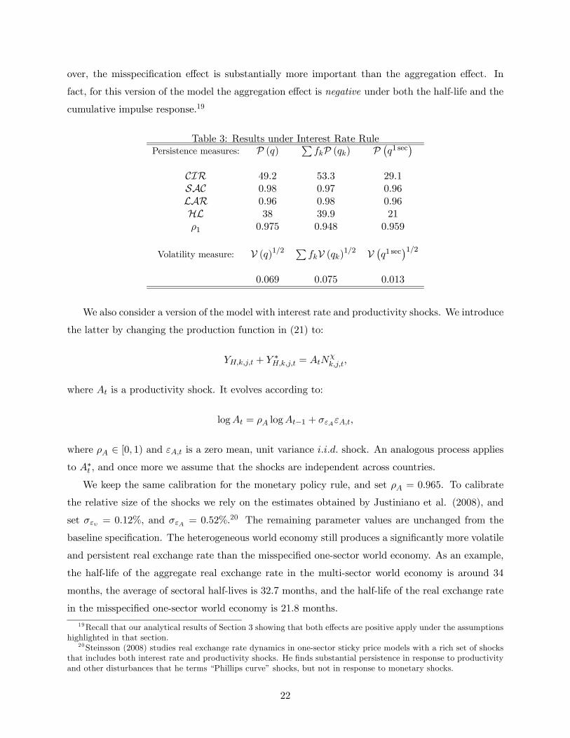
over, the misspecification effect is substantially more important than the aggregation effect. In

fact, for this version of the model the aggregation effect is negative under both the half-life and the

cumulative impulse response.19

Table 3: Results under Interest Rate RulePersistence measures: P (q) P

fkP (qk) P ¡q1 sec¢CIR 49.2 53.3 29.1SAC 0.98 0.97 0.96LAR 0.96 0.98 0.96HL 38 39.9 21ρ1 0.975 0.948 0.959

Volatility measure: V (q)1/2 PfkV (qk)1/2 V ¡q1 sec¢1/2

0.069 0.075 0.013

We also consider a version of the model with interest rate and productivity shocks. We introduce

the latter by changing the production function in (21) to:

YH,k,j,t + Y ∗H,k,j,t = AtNχk,j,t,

where At is a productivity shock. It evolves according to:

logAt = ρA logAt−1 + σεAεA,t,

where ρA ∈ [0, 1) and εA,t is a zero mean, unit variance i.i.d. shock. An analogous process applies

to A∗t , and once more we assume that the shocks are independent across countries.

We keep the same calibration for the monetary policy rule, and set ρA = 0.965. To calibrate

the relative size of the shocks we rely on the estimates obtained by Justiniano et al. (2008), and

set σευ = 0.12%, and σεA = 0.52%.20 The remaining parameter values are unchanged from the

baseline specification. The heterogeneous world economy still produces a significantly more volatile

and persistent real exchange rate than the misspecified one-sector world economy. As an example,

the half-life of the aggregate real exchange rate in the multi-sector world economy is around 34

months, the average of sectoral half-lives is 32.7 months, and the half-life of the real exchange rate

in the misspecified one-sector world economy is 21.8 months.

19Recall that our analytical results of Section 3 showing that both effects are positive apply under the assumptionshighlighted in that section.

20Steinsson (2008) studies real exchange rate dynamics in one-sector sticky price models with a rich set of shocksthat includes both interest rate and productivity shocks. He finds substantial persistence in response to productivityand other disturbances that he terms “Phillips curve” shocks, but not in response to monetary shocks.

22

We also consider several (unreported) alternative calibrations and specifications. We find that

the results with shocks to the interest rate rule and productivity shocks are somewhat more sensitive

to the details of the specification than under nominal income shocks. On the one hand, they are

still robust to the absence of strategic interactions in price setting decisions (i.e., they hold under

strategic neutrality in price setting). On the other, they can be relatively sensitive to the exogenous

persistence of monetary and productivity shocks. The results do naturally vary conditional on each

type of shock. The source of persistence in the interest rate rule - persistent shocks versus interest

rate smoothing - also matters somewhat.21

Uncovering the reasons for such differences in results is an interesting endeavor for future re-

search. In particular, it would be valuable to invest in alternative specifications for the “demand

block” of the model - especially the forward looking “IS curve” - since it has only weak empirical

support (e.g. Fuhrer and Rudebusch 2004). In another direction, while it is a strength that our

model can produce significantly volatile and persistent real exchange rates in response to purely

monetary disturbances, it would be interesting to introduce additional shocks and analyze in more

detail the differences between conditional and unconditional results.22

5 Revisiting the “PPP Strikes Back debate”

Our results uncover an important distinction between the aggregation and the misspecification

effects. In particular, we find that the aggregation effect plays only a minor role in explaining the

persistence of the aggregate real exchange rate in our model. This result may seem at odds with

the findings of Imbs et al. (2005a,b), who estimate an “aggregation bias” and argue that it does

resolve the PPP puzzle. These findings were subject to an intense debate with Engel and Chen

(2005). In this section we revisit the “PPP Strikes Back debate” under the light of our structural

model.

We start by noticing that there is a clear distinction between analytical results and empirical

implementation in the debate between Imbs et al. (2005a,b) and Chen and Engel (2005) on the

importance of heterogeneous sectoral exchange rate dynamics in explaining the PPP puzzle. The

analytical results are illustrated under the assumption that sectoral real exchange rates follow

AR(1) processes, and use the first autocorrelation as a measure of persistence. The comparison

is between the first autocorrelation of the aggregate real exchange rate, and the average of the

21Chari et al.(2002) find that their one-sector sticky price model with a policy rule that features interest ratesmoothing fails to generate reasonable business cycle behavior, in particular in terms of the persistence of deviationsof the real exchange rate from PPP.

22Most of the empirical literature on the dynamics of real exchange rates refers to unconditional results, althoughthere are exceptions, such as Eichenbaum and Evans (1995).

23

first autocorrelations of the underlying sectoral exchange rates. From Lemma 1, the fact that

the first autocorrelation of an AR(1) process equals the autoregressive coefficient implies a zero

misspecification effect under our model. As a result, such comparison would indeed uncover the

aggregation effect.

In contrast, the empirical implementation allows for more general AR(p) processes, and focuses

on non-linear measures of persistence. Moreover, it does not involve a comparison between the

persistence of the aggregate real exchange rate and the average of the persistence of the underlying

sectoral exchange rates. Instead, it compares the former with the persistence based on Mean

Group (MG) estimators for panel data sets with heterogeneous dynamics (Pesaran and Smith 1995).

We show below that, under our structural model with equal sectoral weights, such a comparison

uncovers the sum of the aggregation and misspecification effects, i.e. the total heterogeneity effect.

To be more precise in our description of the empirical implementation of Imbs et al. (2005a,b)

and Chen and Engel (2005), assume that sectoral real exchange rates follow autoregressive processes

of order p (AR (p)), with sector specific coefficients:

qk,t = φk,1qk,t−1 + φk,2qk,t−2 + ...+ φk,pqk,t−p + εk,t,

where εk,t is an i.i.d. shock. The AR (p) real exchange rate process constructed on the basis of the

MG estimators, denoted qMGt , is given by:

qMGt = φMG

1 qt−1 + φMG2 qt−2 + ...+ φMG

p qt−p + εMGt ,

where εMGt is an i.i.d. shock, and φMG

i = 1K

Pk∈K bφk,i, with bφk,i denoting the OLS estimate

of the ith autoregressive coefficient for the kth cross-sectional unit of the panel of sectoral real

exchange rates. In words, qMGt is an AR (p) process with autoregressive coefficients given by the

cross-sectional averages of the (estimated) autoregressive coefficients of the sectoral real exchange

rates, where the averages are taken for each of the p lags. The comparison made in the empirical

implementation of the “aggregation bias” literature is between the estimated persistence of the

aggregate real exchange rate,23 and the persistence of the MG-based real exchange rate.

Strictly speaking, we can refer to such an AR(p) process with the MG autoregressive coefficients

as a misspecified process, in the sense that no single real exchange rate - whether sectoral or

aggregate - actually follows its dynamics.24

An interpretation of the MG-based real exchange rate follows under our structural model and

23Or, alternatively, the persistence estimated from a panel of sectoral exchange rates with methods that imposehomogeneous dynamics across all units of the panel.

24Except in the extremely unlikely case in which one of the sectoral real exchange rates has autoregressive coeffi-cients that exactly coincide with the MG averages.

24

its misspecified one-sector counterpart, in the case of equal sectoral weights. In that case, under

the simplifying assumptions of Subsection 3, sectoral exchange rates follow AR (2) processes:

qk,t = (ρz + λk) qk,t−1 − ρzλkqk,t−2 + ϕkut.

Thus, applying the MG estimator in the population yields ρz +1K

PKk=1 λk as the cross-sectional

average of the first autoregressive coefficients, and −ρz 1KPK

k=1 λk as the cross-sectional average

of the second autoregressive coefficients. It turns out that these are exactly the autoregressive

coefficients of the AR (2) process followed by the aggregate real exchange rate in the misspecified

one-sector world economy. So, the comparison between the persistence of the aggregate real ex-

change rate in the heterogeneous world economy and the persistence implied by the MG estimator

uncovers the total heterogeneity effect rather than the aggregation effect.

5.1 Estimation results and the “PPP Strikes Back debate”

We revisit the “PPP Strikes Back debate” from an empirical perspective, having as a guide the

results of the previous subsection. We start with the Eurostat data used in the estimation of Imbs et

al. (2005a).25 Table 4 presents our replication of some of the results of that paper in the first, third

and fourth columns. The first column shows the results obtained with application of a standard

fixed effects estimator to a panel of aggregate real exchange rates - consisting of up to 19 sectors

for 11 countries, while the last two columns present our results for the simple Mean Group (MG)

estimator of Pesaran and Smith (1995), and for its version with correction for common correlated

effects (MG-CCE).26 The second column, in turn, presents the estimates for the cross-sectional

average across units of the panel. To construct these estimates we run separate OLS regressions

for an AR (19) for each panel unit (sector-country). The choice of lags matches that of the MG

estimators in Imbs et al. (2005a). For the MG-CCE estimator we estimate an AR (12) with 12 lags

for correction for common correlated effects.27 For each of these series, the relevant persistence

statistics are calculated on the basis of the estimated autoregressive coefficients, and then averaged

to yield the result presented in the table.

We focus on the MG-CCE specification highlighted by Imbs et al. (2005a). The results show

that the total heterogeneity effect is indeed very large. Once we account for heterogeneity, the HLgoes from 46 months to 10 months. The aggregation effect is, however, only a small part of this

25The authors make the data available on their websites.26The first and third columns essentially replicate the results in Imbs et al. (2005a) exactly - refer to their Table

II, first line, and Table III line 4. The last column replicates their results on Table III - lines 6 - almost eactly.27 Imbs et al. (2005a) do not mention how many lags they include in the CCE correction terms. We experimented

with different specifications and found these very similar results. For details about the various estimators we referthe reader to Imbs et al. (2005a).

25

Table 4: Decomposition of the Total Heterogeneity Effect - Eurostat DataData Panel, aggregate Panel, sectoral Panel, sectoral Panel, sectoral

Estimation method Fixed Effects OLS MG MG-CCEEqual-weightmodel:

P (q) 1K

PP (qk) P ¡q1 sec¢ P ¡q1 sec¢Persistence measures:

CIR 64.39 59.48 33.19 18.75SAC 0.98 0.97 0.97 .95LAR 0.97 0.94 0.95 0.95HL 46 43.16 26 10

effect. Indeed, the misspecification effect is responsible for 43.16−1046−10 ≈ 92% of the total heterogeneityeffect. For the cumulative impulse response the corresponding figure is 59.48−18.7564.39−18.75 ≈ 89%.28 Theseresults are similar to the ones reported in Section 4, which are based on the solution of our calibrated

model.

To complement our analysis we apply the same estimation methods used for the actual data

to artificial data generated by the model with equal sectoral weights.29 We focus on the case of

strategic neutrality in price setting, since it is the one for which the MG estimators recover the

dynamics of the misspecified one-sector world economy. We generate the data as outlined in footnote

13, and estimate AR processes to obtain the measures of persistence. Under strategic neutrality

we know the exact order of the process followed by each of the variables (from Proposition 1

and Corollaries 1 and 2). For the sectoral exchange rates and for the real exchange rate in the

misspecified one-sector world economy, we fit AR(2) processes. For the aggregate real exchange

rate of the heterogeneous economy, we fit an AR(30) process to approximate the high order ARMA

model.30 We also apply MG estimators to the panel of sectoral exchange rates. For each simulation,

we compute the measures of persistence, and then average across the 150 replications. The results

are presented in Table 5.

The similarity with the results based on actual data is impressive. The total heterogeneity effect

is, again, large: accounting for heterogeneity brings the HL from 52 months to 24.1 months in the

actual one-sector world economy. The MG estimators indeed generate results that are very close

to the misspecified one-sector world economy.

28To replicate the results in Imbs et al. (2005a), in Table 4 we use the actual aggregate series available in Eurostat.To be consistent with our model, we also analyze equally weighted aggregate real exchange rates for each countryconstructed using only the goods that comprise the underlying sectoral panel. Applying a fixed effects estimatorto the resulting panel of country real exchange rates, we estimate a half-life of 39 months. Alternatively, when weestimate separate AR (18) specifications for each country, compute each half-life and then take a simple average, weobtain an average half-life of 43 months.

29We use the model with equal sectoral weights to be consistent with the empirical results of Imbs et al. (2005a).30The results are not very sensitive to increasing the number of lags.

26

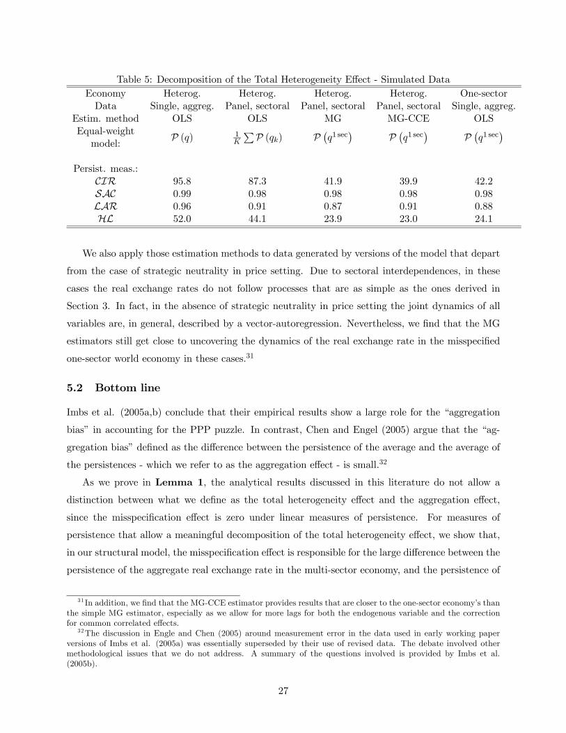
Table 5: Decomposition of the Total Heterogeneity Effect - Simulated DataEconomy Heterog. Heterog. Heterog. Heterog. One-sectorData Single, aggreg. Panel, sectoral Panel, sectoral Panel, sectoral Single, aggreg.

Estim. method OLS OLS MG MG-CCE OLSEqual-weightmodel:

P (q) 1K

PP (qk) P ¡q1 sec¢ P ¡q1 sec¢ P ¡q1 sec¢Persist. meas.:

CIR 95.8 87.3 41.9 39.9 42.2SAC 0.99 0.98 0.98 0.98 0.98LAR 0.96 0.91 0.87 0.91 0.88HL 52.0 44.1 23.9 23.0 24.1

We also apply those estimation methods to data generated by versions of the model that depart

from the case of strategic neutrality in price setting. Due to sectoral interdependences, in these

cases the real exchange rates do not follow processes that are as simple as the ones derived in

Section 3. In fact, in the absence of strategic neutrality in price setting the joint dynamics of all

variables are, in general, described by a vector-autoregression. Nevertheless, we find that the MG

estimators still get close to uncovering the dynamics of the real exchange rate in the misspecified

one-sector world economy in these cases.31

5.2 Bottom line

Imbs et al. (2005a,b) conclude that their empirical results show a large role for the “aggregation

bias” in accounting for the PPP puzzle. In contrast, Chen and Engel (2005) argue that the “ag-

gregation bias” defined as the difference between the persistence of the average and the average of

the persistences - which we refer to as the aggregation effect - is small.32

As we prove in Lemma 1, the analytical results discussed in this literature do not allow a

distinction between what we define as the total heterogeneity effect and the aggregation effect,

since the misspecification effect is zero under linear measures of persistence. For measures of

persistence that allow a meaningful decomposition of the total heterogeneity effect, we show that,

in our structural model, the misspecification effect is responsible for the large difference between the

persistence of the aggregate real exchange rate in the multi-sector economy, and the persistence of

31 In addition, we find that the MG-CCE estimator provides results that are closer to the one-sector economy’s thanthe simple MG estimator, especially as we allow for more lags for both the endogenous variable and the correctionfor common correlated effects.

32The discussion in Engle and Chen (2005) around measurement error in the data used in early working paperversions of Imbs et al. (2005a) was essentially superseded by their use of revised data. The debate involved othermethodological issues that we do not address. A summary of the questions involved is provided by Imbs et al.(2005b).

27

the real exchange rate in the misspecified one-sector world economy. Having our structural model

as a guide, we also show that a similar decomposition is borne out in the data.

The statistical analysis of Imbs et al.’s (2005a) shows that dynamic heterogeneity produces a

large difference between the estimated persistence of aggregate real exchange rates and the per-

sistence implied by MG estimators. In turn, the economically meaningful decomposition of this

difference based on our structural model supports the conclusion that heterogeneity can indeed

account for the PPP puzzle.

6 Conclusion

We show that a multi-sector model with heterogeneity in price stickiness calibrated to match

the microeconomic evidence on price setting in the U.S. economy can produce very volatile and

persistent real exchange rates. In turn, a counterfactual one-sector version of the world economy

that features the same average frequency of price changes fails to do so. We conclude that the

empirical properties of deviations from PPP only warrant the “puzzle” adjective if seen under the

lens of such a one-sector model.

Our findings still leave open a series of important related questions. In our heterogeneous

model, as in the data, aggregate and sectoral real exchange rates are highly persistent, even for

sectors in which prices change quite frequently. Despite the relative uniformity in persistence, the

failure of the one-sector model in matching the data shows that the heterogeneity in the frequency

of price adjustments is crucial for our results. This highlights the importance of investigating

further the reasons for persistence being high across sectors. Our results with the baseline and

alternative specifications point to the importance of the properties of shocks, the nature of the

systematic component of monetary policy, and the details of the “demand side” of our structural

model. There is clearly more work that can be done in this direction.

The large persistence of the aggregate real exchange rate in the multi-sector economy depends

on at least some sectors displaying a low frequency of price adjustment.33 Our calibrated model

features a distribution of the frequency of price changes derived from the recent evidence on price

setting, which documents the existence of sectors in which prices are indeed quite sticky. In this

paper, we highlight the fact that our results hold even in the case of strategic neutrality in price

setting - i.e. when firms’ pricing decisions are unrelated. Thus, we do not explore pricing comple-

mentarities, which are well known to strengthen the real effects of monetary shocks in one-sector

closed economy models (e.g. Woodford 2003, chapter 3). Moreover, as Carvalho (2006) shows, such

33 If the frequency of price changes is uniformly high, the model behaves similarly to a one-sector model with ahigh frequency of price adjustment, and fails to generate volatile and persistent real exchange rates.

28

complementarities amplify the magnitude and persistence of the real effects of monetary shocks even

more in the presence of heterogeneity in price stickiness. The reason is that the sectors in which

prices are relatively more sticky end up having a disproportionate aggregate effect. Thus, such

interdependence in pricing decisions might also have important quantitative effects in terms of real

exchange rate dynamics in the presence of heterogeneity.

For analytical tractability, in this paper we model price stickiness as in Calvo (1983), and assume

that the sectoral frequencies of price adjustment are constant. In closed economies, heterogeneity

in price setting has similar effects in a much larger class of models that includes various sticky price

and sticky information specifications.34 While these results suggest that the nature of nominal

frictions is not a crucial determinant of the effects of heterogeneity, it seems worthwhile to assess

whether the results of this paper do in fact hold in models with different nominal frictions. In

particular, one such class of models involves endogenous, optimal pricing strategies, chosen in the

face of explicit information and/or adjustment costs.35 The importance of our assumption of local

currency pricing, and more generally, the stability of our findings across different policy regimes

can also be assessed with models that feature fully endogenous pricing decisions, along the lines of

Gopinath et al. (2007).

Finally, another important line of investigation refers to the source of heterogeneity in sectoral

exchange rate dynamics. While we emphasize heterogeneity in price stickiness, an additional,

potentially important source of heterogeneity is variation in the dynamic properties of sectoral

shocks. It has been emphasized in recent work on the dynamics of international relative prices

(e.g. Ghironi and Melitz 2005, and Atkeson and Kehoe 2008), but to our knowledge a quantitative

analysis in the context of the PPP puzzle has yet to be undertaken.

34For a detailed analysis of such models, and additional references, see Carvalho and Schwartzman (2008).35More specifically, “menu cost” models (e.g. Barro 1972), models with information frictions as in Reis (2006),

and models with both adjustment and information costs, as in Bonomo and Carvalho (2004).

29

A Appendix

A.1 Proofs of Propositions

Proposition 1 Under the assumptions of Section (3), sectoral real exchange rates follow AR(2)

processes:

(1− ρzL) (1− λkL) qk,t = ϕkut,

where λk ≡ 1 − αk is the per-period probability of no price adjustment for a firm in sector k,

ut ≡ σεz¡εz,t − ε∗z,t

¢is a white noise process, ϕk ≡ λk−(1− λk)

ρzβλk1−ρzβλk , and L is the lag operator.

Proof. From the optimal price equations:

xH,k,t = (1− β (1− αk))Et

X∞s=0

βs (1− αk)s [ct+s + pt+s]

= (1− β (1− αk))Et

X∞s=0

βs (1− αk)s zt+s

= zt +ρzβ (1− αk)

1− β (1− αk) ρz(zt − zt−1) ,

and analogously:

xF,k,t = zt +ρzβ (1− αk)

1− β (1− αk) ρz(zt − zt−1) ,

x∗H,k,t = z∗t +ρzβ (1− αk)

1− β (1− αk) ρz

¡z∗t − z∗t−1

¢,

x∗F,k,t = z∗t +ρzβ (1− αk)

1− β (1− αk) ρz

¡z∗t − z∗t−1

¢.

This implies that the country-sector price indices follow:

pH,k,t = (1− αk) pH,k,t−1 + αk

µzt +

ρzβ (1− αk)

1− β (1− αk) ρz(zt − zt−1)

¶,

pF,k,t = (1− αk) pF,k,t−1 + αk

µzt +

ρzβ (1− αk)

1− β (1− αk) ρz(zt − zt−1)

¶,

p∗H,k,t = (1− αk) p∗H,k,t−1 + αk

µz∗t +

ρzβ (1− αk)

1− β (1− αk) ρz

¡z∗t − z∗t−1

¢¶,

p∗F,k,t = (1− αk) p∗F,k,t−1 + αk

µz∗t +

ρzβ (1− αk)

1− β (1− αk) ρz

¡z∗t − z∗t−1

¢¶,

and that sectoral price indices evolve according to:

pk,t = (1− αk) pk,t−1 + αk

∙zt +

ρzβ (1− αk)

1− β (1− αk) ρz(zt − zt−1)

¸,

p∗k,t = (1− αk) p∗k,t−1 + αk

∙z∗t +

ρzβ (1− αk)

1− β (1− αk) ρz

¡z∗t − z∗t−1

¢¸.

30

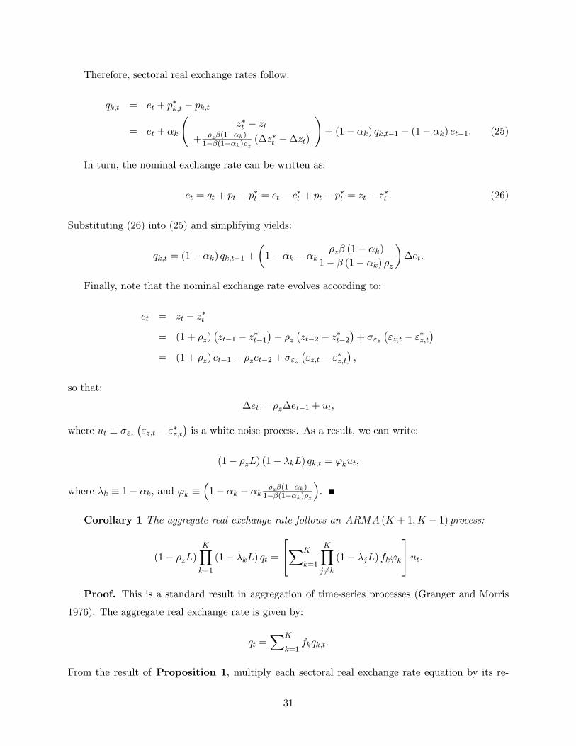
Therefore, sectoral real exchange rates follow:

qk,t = et + p∗k,t − pk,t

= et + αk

Ãz∗t − zt

+ ρzβ(1−αk)1−β(1−αk)ρz (∆z

∗t −∆zt)

!+ (1− αk) qk,t−1 − (1− αk) et−1. (25)

In turn, the nominal exchange rate can be written as:

et = qt + pt − p∗t = ct − c∗t + pt − p∗t = zt − z∗t . (26)

Substituting (26) into (25) and simplifying yields:

qk,t = (1− αk) qk,t−1 +µ1− αk − αk

ρzβ (1− αk)

1− β (1− αk) ρz

¶∆et.

Finally, note that the nominal exchange rate evolves according to:

et = zt − z∗t

= (1 + ρz)¡zt−1 − z∗t−1

¢− ρz¡zt−2 − z∗t−2

¢+ σεz

¡εz,t − ε∗z,t

¢= (1 + ρz) et−1 − ρzet−2 + σεz

¡εz,t − ε∗z,t

¢,

so that:

∆et = ρz∆et−1 + ut,

where ut ≡ σεz¡εz,t − ε∗z,t

¢is a white noise process. As a result, we can write:

(1− ρzL) (1− λkL) qk,t = ϕkut,

where λk ≡ 1− αk, and ϕk ≡³1− αk − αk

ρzβ(1−αk)1−β(1−αk)ρz

´.

Corollary 1 The aggregate real exchange rate follows an ARMA (K + 1,K − 1) process:

(1− ρzL)KYk=1

(1− λkL) qt =

⎡⎣XK

k=1

KYj 6=k

(1− λjL) fkϕk

⎤⎦ut.Proof. This is a standard result in aggregation of time-series processes (Granger and Morris

1976). The aggregate real exchange rate is given by:

qt =XK

k=1fkqk,t.

From the result of Proposition 1, multiply each sectoral real exchange rate equation by its re-

31

spective sectoral weight to obtain:

fk (1− ρzL) (1− λkL) qk,t = fkϕkut.

Multiplying each such equation by all (K − 1) L-polinomials of the form (1− λmL) , m 6= k and

adding them up yields:

(1− ρzL)KYk=1

(1− λkL) qt =

⎡⎣XK

k=1

KYm6=k

(1− λmL) fkϕk

⎤⎦ut,so that qt follows an ARMA (K + 1,K − 1).

Corollary 2 The aggregate real exchange rate of the misspecified one-sector world economy

follows an AR (2) process:

(1− ρzL)¡1− λL

¢q1 sect = ϕut,

where λ ≡PKk=1 fkλk and ϕ ≡ λ− ¡1− λ

¢ ρzβλ

1−ρzβλ.

Proof. FromCorollary 1, the real exchange rate in a one-sector world economy with frequency

of price changes equal to α - probability of no-adjustment equal to λ = 1− α - follows:

(1− ρzL)¡1− λL

¢qt =

¡1− λL

¢µλ− ¡1− λ

¢ ρzβλ

1− ρzβλ

¶ut.

Proposition 2 For the measures of persistence P = CIR,LAR,SAC:

P (q) > P ¡q1 sec¢ .Proof. We prove separate results for each measure of persistence.

CIR:Recall that we denote the impulse response function of the qt process to a unit impulse by

IRFt (q). In turn, let SIRFt (q) denote the “scaled impulse response function,” i.e. the im-

pulse response function to one standard deviation shock. Since qt =PK

k=1 fkqk,t, SIRFt (q) =PKk=1 fkSIRFt (qk). So, the impulse response function of the qt process to a unit impulse, which is

simply the scaled impulse response function normalized by the initial impact of the shock, can be

written as:

IRFt (q) =

PKk=1 fkSIRFt (qk)PKk=1 fkSIRF0 (qk)

. (27)

32

From (27), the cumulative impulse response for qt is:

CIR (q) =X∞

t=0IRFt (q) =

PKk=1 fk

P∞t=0 SIRFt (qk)PK

k=1 fkSIRF0 (qk). (28)

From the processes in Proposition 1 we can computeP∞

t=0 SIRFt (qk), and SIRF0 (qk):X∞t=0

SIRFt (qk) =λk (1− ρzβ)

1− ρzβλk

1

(1− λk) (1− ρz), (29)

SIRF0 (qk) =λk (1− ρzβ)

1− ρzβλk. (30)

Substituting (29) and (30) into (28) yields:

CIR (q) =PK

k=1 fkλk(1−ρzβ)1−ρzβλk

1(1−λk)(1−ρz)PK

k=1 fkλk(1−ρzβ)1−ρzβλk

.

Note that λk(1−ρzβ)1−ρzβλk is increasing in λk, so that efk ≡ fk

λk(1−ρzβ)1−ρzβλk

Kk=1 fk

λk(1−ρzβ)1−ρzβλk

are sectoral weights ob-

tained through a transformation of fk, which attaches higher weight to higher λk’s. The fact that1

(1−λk)(1−ρz) is also increasing, and moreover convex, in λk thus implies the following inequalities:

XK

k=1efk 1

(1− λk) (1− ρz)| {z }CIR(q)

>XK

k=1fk

1

(1− λk) (1− ρz)| {z }Kk=1 fkCIR(qk)

>1PK

k=1 fk (1− λk) (1− ρz)| {z }CIR(q1 sec)

. (31)

This proves that CIR (q) > CIR ¡q1 sec¢.LAR:We order the sectors in terms of price stickiness, starting from the most flexible: αk > αk+1

(λk < λk+1). Moreover, recall that we assume ρz ∈ (1− α1, 1− αK). Thus, based on Proposition

1 and Corollaries 1 and 2, we obtain directly the following results:

LAR (q) = λK ,

LAR (qk) = max {λk, ρz} ,LAR ¡q1 sec¢ = max

©λ, ρz

ª= max

½XK

k=1fkλk, ρz

¾.

Therefore:

LAR (q) >XK

k=1fkLAR (qk) > LAR

¡q1 sec

¢. (32)

SAC:

33

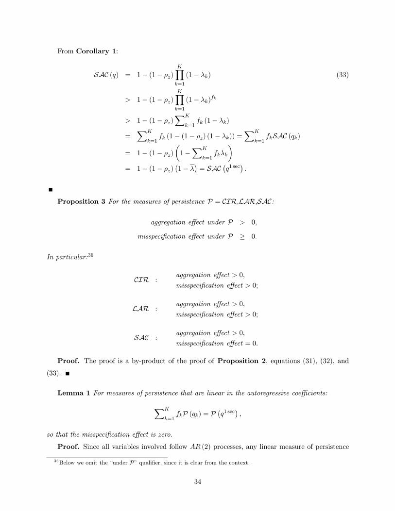
From Corollary 1:

SAC (q) = 1− (1− ρz)KYk=1

(1− λk) (33)

> 1− (1− ρz)KYk=1

(1− λk)fk

> 1− (1− ρz)XK

k=1fk (1− λk)

=XK

k=1fk (1− (1− ρz) (1− λk)) =

XK

k=1fkSAC (qk)

= 1− (1− ρz)

µ1−

XK

k=1fkλk

¶= 1− (1− ρz)

¡1− λ

¢= SAC ¡q1 sec¢ .

Proposition 3 For the measures of persistence P = CIR,LAR,SAC:

aggregation effect under P > 0,

misspecification effect under P ≥ 0.

In particular:36

CIR :aggregation effect > 0,

misspecification effect > 0;

LAR :aggregation effect > 0,

misspecification effect > 0;

SAC :aggregation effect > 0,

misspecification effect = 0.

Proof. The proof is a by-product of the proof of Proposition 2, equations (31), (32), and

(33).

Lemma 1 For measures of persistence that are linear in the autoregressive coefficients:

XK

k=1fkP (qk) = P

¡q1 sec

¢,

so that the misspecification effect is zero.

Proof. Since all variables involved follow AR (2) processes, any linear measure of persistence

36Below we omit the “under P” qualifier, since it is clear from the context.

34

is characterized by two real numbers c1 and c2, such that the persistence for any given process

equals the inner product between these two numbers and the two autoregressive coefficients. From

Proposition 1, the persistence of qk,t under a linear measure is thus:

P (qk) = c1 (ρz + λk)− c2 (ρzλk) .

The weighted average of sectoral persistences is then:

XK

k=1fkP (qk) =

XK

k=1fk (c1 (ρz + λk)− c2 (ρzλk))

= c1

µρz +

XK

k=1fkλk

¶− c2

µρzXK

k=1fkλk

¶= c1

¡ρz + λ

¢− c2¡ρzλ

¢= P ¡q1 sec¢ .

Proposition 4 Let V (qk) denote the unconditional variance of the qk,t process. Then:XK

k=1fkV (qk) > V

¡q1 sec

¢.

Proof. We prove that V (qk) is convex in λk. From Proposition 1, the variance of qk,t is:

V ar (qk,t) =(1 + ρzλk)ϕ

2kσ2εz

(1− ρzλk)h(1 + ρzλk)

2 − (ρz + λk)2i ,

where ϕk ≡ λk − (1− λk)ρzβλk1−ρzβλk . We differentiate twice with respect to λk, and show that the

result is positive. Due to the extremely long resulting expressions, for these steps we rely on

Wolfram Mathematica, by Wolfram Research. The code file is available upon request.

Proposition 5 Under the assumptions of Subsection 3.3:

Vµ1

K

XK

k=1qk,t

¶−→K→∞

∞,

CIR

µ1

K

XK

k=1qk,t

¶−→K→∞

∞,

V ¡q1 sec¢ , CIR ¡q1 sec¢ <∞.

Proof. For convenience, we reproduce here the required assumptions. The frequency of price

changes αk for each new sector is drawn from (0, 1− δ) for arbitrarily small δ > 0, according to some

distribution with density g (α|b), where α is the frequency of price changes and b is a parameter.

For α ≈ 0 such density is assumed to be approximately proportional to α−b, with b ∈ ¡12 , 1¢.Moreover, it yields a strictly positive average frequency of price changes: α =

R 1−δ0 g (α|b)αdα > 0.

35

For simplicity we focus on the case of ρz = 0, and then extend the argument to the general case.

For each qk,t process (1− λkL) qk,t = ϕkut with ϕk ≡ λk and αk = 1− λk drawn from g (α|b),define an auxiliary eqk,t process satisfying:

(1− λkL) eqk,t = eϕut,where eϕ < δ. Since eϕ is independent of λk, these eqk,t processes satisfy the assumptions in Zaffaroni(2004), and application of his Theorem 4 yields:

Vµ1

K

XK

k=1eqk,t¶ −→

K→∞∞.

Finally, since the αk’s have support (0, 1− δ) for small δ > 0, V³1K

PKk=1 qk,t

´> V

³1K

PKk=1 eqk,t´,

which proves that V³1K

PKk=1 qk,t

´−→K→∞

∞. Analogously, application of Zaffaroni’s (2004) resultto the spectral density of the limiting process at frequency zero shows that it is unbounded. In

turn, the fact that the spectral density at frequency zero for AR (p) processes is an increasing

monotonic transformation of the cumulative impulse response (e.g. Andrews and Chen 1994)

implies CIR³1K

PKk=1 qk,t

´−→K→∞

∞.The results for the real exchange rate in the limiting misspecified one-sector world economy

follow directly from the fact that α =R 1−δ0 g (α|b)αdα > 0, so that it follows a stationary AR

process.

Finally, Zaffaroni’s (2004) extension of his results to ARMA (p, q) processes implies thatPropo-

sition 5 also holds for ρz > 0.

36

References

[1] Abadir, K. and G. Talmain (2002), “Aggregation, Persistence and Volatility in a Macro Model,”

Review of Economic Studies 69: 749-779.

[2] Andrews, D. and H. Chen (1994), “Approximately Median-Unbiased Estimation of Autore-

gressive Models,” Journal of Business & Economic Statistics 12: 187-204.

[3] Atkeson, A. and A. Burstein (2008), “Pricing-to-Market, Trade Costs, and International Rel-

ative Prices,” American Economic Review, forthcoming.

[4] Ball, L. and D. Romer (1990), “Real Rigidities and the Non-Neutrality of Money,” Review of

Economic Studies 57: 183-203.

[5] Barro, R. (1972), “A Theory of Monopolistic Price Adjustment,” Review of Economic Studies

39: 17-26.

[6] Benigno, G. (2004), “Real Exchange Rate Persistence and Monetary Policy Rules,” Journal

of Monetary Economics 51: 473-502.

[7] Bergin, P. and R. Feenstra (2001), “Pricing-to-Market, Staggered Contracts, and Real Ex-

change Rate Persistence,” Journal of International Economics 54: 333—359.

[8] Bils, M. and P. Klenow (2004), “Some Evidence on the Importance of Sticky Prices,” Journal

of Political Economy 112: 947-985.

[9] Bonomo, M. and C. Carvalho (2004), “Endogenous Time-Dependent Rules and Inflation Iner-

tia,” Journal of Money, Credit and Banking 36: 1015-1041.

[10] Calvo, G. (1983), “Staggered Prices in a Utility Maximizing Framework,” Journal of Monetary

Economics 12: 383-98.

[11] Carvalho, C. (2006), “Heterogeneity in Price Stickiness and the Real Effects of Monetary

Shocks,” Frontiers of Macroeconomics: Vol. 2: Iss. 1, Article 1.

[12] Carvalho, C. and F. Schwartzman (2008), “Heterogeneous Price Setting Be-

havior and Aggregate Dynamics: Some General Results,” mimeo available at

http://www.princeton.edu/~cvianac/research.html.

[13] Chari, V., P. Kehoe, and E. McGrattan (2002), “Can Sticky Price Models Generate Volatile

and Persistent Real Exchange Rates?,” Review of Economic Studies, 69: 533-63.

37

[14] Chen, S. and C. Engel (2005), “Does ‘Aggregation Bias’ Explain the PPP Puzzle?,” Pacific

Economic Review 10: 49-72.

[15] Dhyne, E., L. Álvarez, H. Le Bihan, G. Veronese, D. Dias, J. Hoffman, N. Jonker, P. Lünne-

mann, F. Rumler and J. Vilmunen (2006), “Price Changes in the Euro Area and the United

States: Some Facts from Individual Consumer Price Data,” Journal of Economic Perspectives

20: 171-192.

[16] Eichenbaum, M. and C. Evans (1995), “Some Empirical Evidence on the Effects of Monetary

Shocks on Exchange Rates,” Quarterly Journal of Economics 110: 975-1010.

[17] Fuhrer, J. and G. Rudebusch (2004), “Estimating the Euler Equation for Output,” Journal of

Monetary Economics 51: 1133-1153.

[18] Gagnon, E. (2007), “Price Setting During Low and High Inflation: Evidence from Mexico,”

International Finance Discussion Papers 896, Board of Governors of the Federal Reserve Sys-

tem.

[19] Ghironi, F. and M. Melitz (2005), “International Trade and Macroeconomic Dynamics with

Heterogeneous Firms,” Quarterly Journal of Economics 120: 865-915.

[20] Granger, C. (1980), “Long Memory Relashionships and the Aggregation of Dynamic Models,”

Journal of Econometrics 14: 227-238.

[21] Granger, C and R. Joyeux (1980), “An Introduction to Long Memory Time Series Models and

Fractional Differencing,” Journal of Time Series Analysis 1: 15-29.

[22] Granger, C. and M. Morris (1976), “Time Series Modelling and Interpretation,” Journal of

the Royal Statistical Society, Series A, Vol. 139: 246-257.

[23] Gopinath, G., O. Itskhoki, and R. Rigobon (2007), “Currency Choice and Exchange Rate

Pass-through,” NBER Working Paper 13432.

[24] Gopinath, G. and R. Rigobon (2008), “Sticky Borders,” Quarterly Journal of Economics,

forthcoming.

[25] Imbs, J., H. Mumtaz, M. Ravn and H. Rey (2005a), “PPP Strikes Back: Aggregation and the

Real Exchange Rate,” Quarterly Journal of Economics 120: 1-43.

[26] (2005b), “‘Aggregation Bias’ DOES Explain the PPP Puzzle,” NBERWorking

Paper 11607.

38

[27] Justiniano, A., G. Primiceri, and A. Tambalotti (2008), “Investment Shocks and Business

Cycles,” mimeo available at http://faculty.wcas.northwestern.edu/~gep575/research.html.

[28] Kehoe, P. and V. Midrigan (2007), “Sticky Prices and Sectoral Real Exchange Rates,” Federal

Reserve Bank of Minneapolis Working Paper 656.

[29] Mankiw, G. and R. Reis (2002), “Sticky Information Versus Sticky Prices: A Proposal to

Replace the New Keynesian Phillips Curve,” Quarterly Journal of Economics 117: 1295-1328.

[30] Nakamura, E. and J. Steinsson (2007), “Five Facts About Prices: A Reevaluation of Menu

Cost Models,” mimeo available at http://www.columbia.edu/~en2198/papers.html.

[31] Pesaran, M. and R. Smith (1995), “Estimating Long-Run Relationships from Dynamic Het-

erogeneous Panels,” Journal of Econometrics 68: 79-113.

[32] Reis, R. (2006), “Inattentive Producers,” Review of Economic Studies 73: 793-821.

[33] Rogoff, K. (1996), “The Purchasing Power Parity Puzzle,” Journal of Economic Literature 34:

647—668.

[34] Steinsson, J. (2008), “The Dynamic Behavior of the Real Exchange Rate in Sticky-Price Mod-

els,” American Economic Review 98: 519-533.

[35] Woodford, M. (2003), Interest and Prices: Foundations of a Theory of Monetary Policy,

Princeton University Press.

[36] Zaffaroni, P. (2004), “Contemporaneous Aggregation of Linear Dynamic Models in Large

Economies,” Journal of Econometrics 120: 75-102.

39