Aggregative Disequilibrium Econometric Modelsof the Labour Market

with Macroeconomic Shocksand Discouraged Workers

by

Vassilis A. HajivassiliouDepartment of EconomicsLondon School of Economics

Revised February 2019

Abstract

In this paper, I rst show how aggregation over submarkets that ex-hibit varying degrees of disequilibrium can provide a foundation to the clas-sic \short-side" disequilibrium econometric model of Fair and Jaee [12]. Ithen introduce explicit randomness in the aggregative model as arising fromeconomy-wide demand and supply shocks, which are allowed to be seriallycorrelated. The model makes explicit allowance for the discouraged workerphenomenon, whereby labour supply endogenizes the probability of excesssupply prevailing in the market.I apply suitable simulation estimation methods to circumvent hitherto

intractable computational problems resulting from serial correlation in theunobservables in disequilibrium analysis. I show that the introduction ofmacroeconomic shocks has fundamentally dierent implications compared tothe traditional approach that arbitrarily appends an additive disturbanceterm to the basic equation of the model.The aggregative disequilibrium model with macroeconomic shocks and

the discouraged worker eect is estimated from a set of quarterly observationson the labour market in US manufacturing. A major nding is that theintroduction of macroeconomic shocks is able to explain a large part of theresidual serial correlation that was plaguing traditional studies. Moreover,the new modelling technique yields considerably more satisfactory estimates

of the supply side of the markets.Laroque and Salanie papers: add referencesAdd idea of Eaton and Quandt. My related ideas and

aggregation

E-mail: vassilis@econ.lse.ac.ukAddress: Department of Economics

London School of EconomicsHoughton StreetLondon WC2A 2AE

Keywords: Disequilibrium, Aggregation, Simulation Estimation Methods, DynamicLimited Dependent Variable Models, Labor Markets, Discouraged WorkerEect

JEL Classication: 210, 820

1

Aggregative Disequilibrium Econometric Modelsof the Labour Market

with Macroeconomic Shocksand Discouraged Workers

1 Introduction

Aggregation over submarkets that exhibit varying degrees of disequilibrium has a long tradi-tion in economics. Since the pioneering work of Malinvaud [27] and Muellbauer [30], severalauthors have offered variations on the same theme. See, inter alia, Lambert [22], Kooiman[20], Andrews and Nickell [4], Hajivassiliou [18], and Quandt [35]. The basic aggregationapproach has been proposed as providing a more disaggregated foundation to the classic“short-side” disequilibrium model of Fair and Jaffee [12]. See also Goldfeld and Quandt[13], Rosen and Quandt [40], and Quandt [34]. Moreover, estimation of a version of theaggregative model (Hajivassiliou [18]) only requires non-linear least squares with correctionfor conditional heteroskedasticity, thus circumventing some of the more severe computationalproblems of the ML estimation of the classic model.

In this paper, I introduce explicit randomness in the deterministic aggregation model asarising from economy-wide demand and supply shocks. I then show that this has fundamen-tally different implications compared to the traditional approach that arbitrarily appendsan additive disturbance term to the basic equation of the model. The second innovationin this paper is to introduce simulation estimation methods, pioneered by McFadden [29],Pakes and Pollard [32], Laroque and Salanie [23], and Laroque and Salanie [24],to allow forserial correlation in the economy-wide demand and supply shocks. Such modelling is notfeasible by traditional estimation methods because the non-linearity of the model would leadto intractable integrals.

The aggregative disequilibrium model with macroeconomic shocks is then estimated froma data set consisting of quarterly observations on the labour market in US manufacturing. Amajor finding is that the introduction of macroeconomic shocks is able to explain a large partof the hitherto unexplainable residual serial correlation that was plaguing traditional studies.Moreover, the new modelling technique yields considerably more satisfactory estimates ofthe supply side of the markets.

In Section 2 I present the aggregative disequilibrium model with macroeconomic shocksand contrast it to previous approaches. A maximum likelihood estimation procedure is pro-posed and analyzed. Technical details are given in Appendix A. Section 3 shows how tomake explicit allowance for the “discouraged worker phenomenon,” whereby labour supplyendogenizes the probability of excess supply prevailing in the market. Section 4 presents thesimulation estimation method that allows me to introduce serially correlated macroeconomicshocks in the aggregative disequilibrium model. The consistency and asymptotic normalityof the simulation estimation method is also discussed in that Section. Section 5 describesthe specifications of the sectoral demand and supply functions used in the empirical imple-mentations. The quarterly data set used in this study is described in Section 6 and DataAppendix B. Section 7 discusses some preliminary issues in econometric implementation of

2

aggregative disequilibrium models. Section 8 presents the empirical results. Concludingremarks are given in Section 9.

2 Macroeconomic Shocks and Aggregation

Think of the economy or the relevant market as consisting of J sectors assumed of equalsize for simplicity; otherwise simple scale factors are needed. In sector j, j = 1, · · · , J ,notional demand and supply are denoted by Dj

t and Sjt respectively, and, by the “short-

side” rule of voluntary exchange (see Barro and Grossman [5]), transacted quantity is givenby Qj

t = min(Djt , S

jt ). Hence,

Djt = Dt + εj

t (1)

Sjt = St + uj

t (2)

Qjt = min(Dj

t , Sjt ), (3)

where Dt(= Xdt βd + ηt ≡ D∗

t + ηt) and St(= Xst β

s + θt ≡ S∗t + θt) are to be thought ofas mean (economy-wide) demands and supplies, and εj, uj are sector-specific demand andsupply shocks. ηt and θt are unobservable economy-wide shocks. Dropping the time subscriptfor simplicity, I aggregate over sectors on the basis of a postulated distribution function of theshocks F (ε, u|η, θ), conditioning on the temporal (economy-wide) randomness included in Dt

and St in the form of ηt and θt. Note the lack of a j index, implying that the sector-specificshocks are drawn from an identical distribution, the drawings assumed independent acrossj.1 As Muellbauer [30] shows, given condition (3), transacted quantity in the aggregate,conditional on the macro economic shocks ηt and θt, is given by

(Q|η, θ) =∑

j∈Dj<SjDj +

∑

j∈Dj>SjSj. (4)

Let A be the set of sectors that are in excess demand, i.e., j|Dj > Sj ≡ A and let B beits complement j|Dj < Sj ≡ B. Making the assumption of many markets so as to give anapproximately continuous distribution F (·, ·|η, θ), we can replace summations by integralsto obtain

(Q|η, θ) =∫

BDjdF (ε, u|η, θ) +

∫

ASjdF (ε, u|η, θ)

=∫

B(D + εj)dF (ε, u|η, θ) +

∫

A(S + uj)dF (ε, u|η, θ)

=∫

BDdF (ε, u|η, θ) +

∫

ASdF (ε, u|η, θ) +

∫

Bε dF (ε, u|η, θ) +

∫

Au dF (ε, u|η, θ)

= D∫

BdF (ε, u|η, θ) + S

∫

AdF (ε, u|η, θ) + ε + u

= D · (1− π) + S · π + ε + u, (5)

1This independence of shocks across j might appear restrictive, given, for example the presence of macro-economic shocks. Recall, however, that we are for the moment conditioning on such economy-wide shocks.Some of these shocks can be captured by the inclusion of economy-wide variables in D∗

t and S∗t , e.g., moneysupply. Below, I investigate explicitly the effects of the randomness in the macroeconomic shocks ηt and θt.

3

where π is the proportion of the sectors that are in excess demand. The error term εdenotes the average demand shock in the sectors that are in excess supply and u the averagesupply shock in sectors with excess demand. The proportion π is clearly dependent uponthe magnitude of total excess demand D − S ≡ (D∗ − S∗ + η − θ) through the conditionaldensity function dF (ε, u|η, θ), and so are ε and u.

Hence, we see that under appropriate conditions, aggregating over micro-sectors in dis-equilibrium while conditioning on macroeconomic shocks predicts that transacted quantitywill be given by the total mean demand and demand shocks weighted by the proportionof sectors in excess supply, plus the total mean supply and supply shocks weighted by theproportion of sectors in excess demand. In an exactly analogous manner, in the case ofthe switching approach on a single market, expected transacted quantity is given by theconvex combination of expected demand and expected demand-error, given excess supplyon one hand, and the expected supply plus the expected supply-error, given excess demandon the other. The weighting factor is in this case the probability of the single sector be-ing in excess demand. Figure 1 summarizes the main result of this aggregation theory.

EQ

p

Q

D

S

Figure 1

Now consider explicitly the implications of the presence of the macroeconomic shocks η and

θ. Assume that η and θ are jointly normal with covariance matrix Ωηθ and i.i.d. acrosstime. Also assume that the sectoral shocks ε and u are normally distributed and denote theexcess demand variance by σ2 ≡ V (ε − u). Such normality assumptions are customary inthe literature. In summary,

(ηθ

)∼ N

((00

),[σ2

η σηθ

σ2θ

]), and

(εu

)∼ N

((00

),[σ2

ε σεu

σ2u

]). (6)

Denote by P (A) the probability of excess demand conditional on the macro shocks η and θ.

4

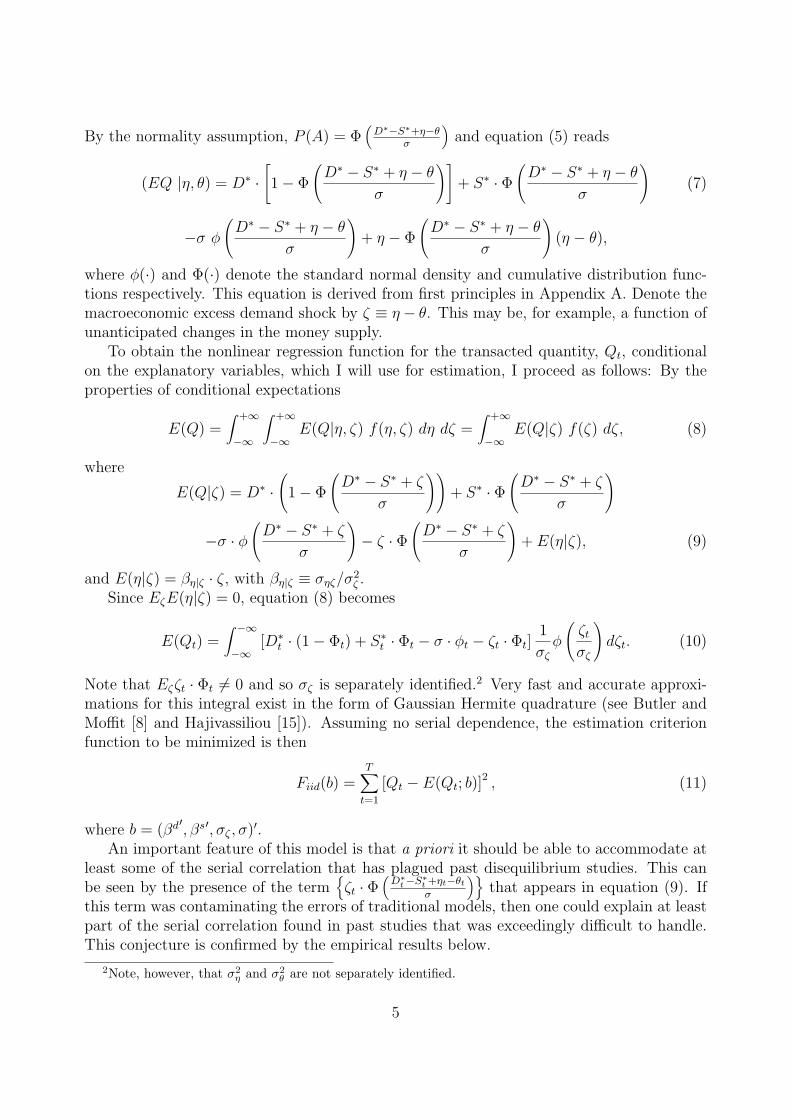
By the normality assumption, P (A) = Φ(

D∗−S∗+η−θσ

)and equation (5) reads

(EQ |η, θ) = D∗ ·[1− Φ

(D∗ − S∗ + η − θ

σ

)]+ S∗ · Φ

(D∗ − S∗ + η − θ

σ

)(7)

−σ φ

(D∗ − S∗ + η − θ

σ

)+ η − Φ

(D∗ − S∗ + η − θ

σ

)(η − θ),

where φ(·) and Φ(·) denote the standard normal density and cumulative distribution func-tions respectively. This equation is derived from first principles in Appendix A. Denote themacroeconomic excess demand shock by ζ ≡ η − θ. This may be, for example, a function ofunanticipated changes in the money supply.

To obtain the nonlinear regression function for the transacted quantity, Qt, conditionalon the explanatory variables, which I will use for estimation, I proceed as follows: By theproperties of conditional expectations

E(Q) =∫ +∞

−∞

∫ +∞

−∞E(Q|η, ζ) f(η, ζ) dη dζ =

∫ +∞

−∞E(Q|ζ) f(ζ) dζ, (8)

where

E(Q|ζ) = D∗ ·(

1− Φ

(D∗ − S∗ + ζ

σ

))+ S∗ · Φ

(D∗ − S∗ + ζ

σ

)

−σ · φ(

D∗ − S∗ + ζ

σ

)− ζ · Φ

(D∗ − S∗ + ζ

σ

)+ E(η|ζ), (9)

and E(η|ζ) = βη|ζ · ζ, with βη|ζ ≡ σηζ/σ2ζ .

Since EζE(η|ζ) = 0, equation (8) becomes

E(Qt) =∫ −∞

−∞[D∗

t · (1− Φt) + S∗t · Φt − σ · φt − ζt · Φt]1

σζ

φ

(ζt

σζ

)dζt. (10)

Note that Eζζt · Φt 6= 0 and so σζ is separately identified.2 Very fast and accurate approxi-mations for this integral exist in the form of Gaussian Hermite quadrature (see Butler andMoffit [8] and Hajivassiliou [15]). Assuming no serial dependence, the estimation criterionfunction to be minimized is then

Fiid(b) =T∑

t=1

[Qt − E(Qt; b)]2 , (11)

where b = (βd′, βs′, σζ , σ)′.An important feature of this model is that a priori it should be able to accommodate at

least some of the serial correlation that has plagued past disequilibrium studies. This canbe seen by the presence of the term

ζt · Φ

(D∗t−S∗t +ηt−θt

σ

)that appears in equation (9). If

this term was contaminating the errors of traditional models, then one could explain at leastpart of the serial correlation found in past studies that was exceedingly difficult to handle.This conjecture is confirmed by the empirical results below.

2Note, however, that σ2η and σ2

θ are not separately identified.

5

3 Modelling the Discouraged Worker Effect

A well-documented phenomenon for markets with binding quantity constraints is that par-ticipants respond endogenously to the probability of a constraint binding. For example, insituations with significant liquidity constraints affecting consumer behaviour, an importantfinding (Grant 2002, Jappelli 1990 etc.) is that the more poorly educated people, householdsheaded by women, and ethnic minorities housholds are less likely to hold debt and less likelyto face binding liquidity constraints seems rather odd at first glance. In this section we offeran explanation of such findings by making the probability of encountering a binding liquidityconstraint affect a household’s notional demand for credit. This feature of our model allowsexplicitly that people who realize rationally that based on their characteristics they are verylikely to face a binding constraint (e.g., uneducated people, and households headed by womenor minorities), such people may feel discouraged from applying for credit in the first place.This “discouragement effect” on an individual’s demand for credit implies a certain fixedpoint between the probability of a binding credit constraint entering Demand and the overalprobability of S=min(D,S) (i.e., the prob of the credit constraint binding) taking place inthe credit market at that time.

In greater detail:

D = Xdβd + γ × Prob(D > S) + εd, S = Xsδs + εs

whereProb(D > S) = Prob(εs − εd < Xdβd − γ × Prob(D > S)−Xsδs

It should be noted that this modelling device is in the spirit of Eaton and Quandt [10].

4 Simulation Estimation Methods and Serially Corre-

lated Macroeconomic Shocks

One would expect, a priori, that the macroeconomic shocks η and θ introduced in theprevious section are serially correlated because such shocks typically incorporate the effects ofgovernment macroeconomic monetary and fiscal policy and the general real and nominal stateof the economy. With classical econometric methods, however, allowing for this possibilityleads to intractable computational problems. See, for example, Laroque and Salanie [24] andRichard [37] for a discussion of this issue.

To be more specific, recall equation (7), which describes the conditional expectation ofthe transacted quantity in the economy, Q, given the evolution of the macroeconomic shocksη and θ. Assuming that these errors are i.i.d. over time as in (6), I was able to show that theexpected value of Q can be obtained by expression (10), which can be evaluated by numericalquadrature techniques. Assume now instead that the errors follow the bivariate stationaryGaussian AR(1) process:

ηt = ρηηt−1 + νt |ρη| < 1

θt = ρθθt−1 + µt |ρθ| < 1(12)

6

Given that the macro shocks appear non-linearly in the regression function (7), efficientclassical estimation would require integration of order T ≈ 140.

E(Q1, · · · , QT ) =∫ −∞

−∞· · ·

∫ −∞

−∞E(Q1, · · · , QT |η1, ζ1, · · · , ηT , ζT ) f(η1, ζ1, · · · , ηT , ζT ) dη1 dζ1 · · · dηT dζT

=∫ −∞

−∞· · ·

∫ −∞

−∞

T∏

t=1

E(Qt|η1, ζ1, · · · , ηT , ζT ) f(η1, ζ1, · · · , ηT , ζT ) dη1 dζ1 · · · dηT dζT (13)

Given that all E(Qt| · · ·) terms are interdependent because (ηt, θt) are serially correlated,this integral cannot be reduced to a product of univariate integrals.

To overcome this problem, one can use the following simulation estimation procedure:3

Given a trial set of parameter values for β’s, ρ′s, σ’s etc., and a set of initial conditionsη0, θ0, we draw R sequences of ηt, θtT

t=1 and calculate the implied R sequences for theendogenous variable Q of the system, say R sequences Qr

t (b)Tt=1, r = 1, · · · , R. The em-

pirical average 1R

∑Rr=1 Qr

t (b) will be an unbiased and consistent simulator for EQt(b). Thecontinuity of the function E(Q|b, η, θ) together with the mixing property of the macro shocksη and θ, implies that the distribution of Q will be mixing as well. Then, minimizing withrespect to the parameters b the quadratic distance between Q and the average of Q oversimulations

FAR1(b) =T∑

t=1

[Qt − 1

R

∑r

Qrt (b)

]2

, (14)

defines a consistent and asymptotically normal estimator for the parameter vector b, providedR rises at least as fast as

√T . This follows from results in Andrews [3] on empirical process

theorems on serially dependent processes.4 See also Laroque and Salanie [23] and Salanie [41]for the use of simulation estimation methods to facilitate the estimation of disequilibriummodels.5

5 Data

In this paper, the market under examination is the aggregate labour market in the U.S. man-ufacturing sector and the period covered is 1948QI–1983QII. The data used are seasonallyunadjusted quarterly series contained in the CITIBANK data base, compiled by the Councilof Economic Advisers, or compiled by the Federal Reserve Board. Details are provided inAppendix B.

3Such a simulation estimation method was independently proposed and evaluated in a Monte Carlo studyby Laroque and Salanie [24].

4An important caveat is that to my knowledge all asymptotic results for simulation estimators assumemixing processes. In practice, however, macroeconomic time series tend to be non-stationary. It is not clearwhether or not the stationary results can be extended to the non-stationary case.

5Notice that the aggregation approach adopted here avoids a key difficulty of typical disequilibrium modelsand other limited dependent variable models, because the quantity I simulate is continuously differentiablein both the parameters and the errors that are being simulated. Other simulation estimation methods fordisequilibrium models, e.g., Laroque and Salanie [23], are only piece-wise continuously differentiable. Thenumber of simulations, R, I used below was 100.

7

6 Specification of Demand and Supply

6.1 Demand:

The most general specification I tried was the following (in logarithmic form):

D∗t = a0 +a′1 · seasonal dummies+a2 ·T+a3 ·Wt +a4 ·Yt +a5 ·Wt−1 +a6 ·Yt−1 +a7 ·W∗t . (15)

This corresponds to the marginal productivity condition of cost-minimization of the neoclas-sical firm. W is the (gross) real wage. I tried both deflating by the CPI index and by thetheoretically more relevant WPI deflator.

Y is industrial production and T is a time trend supposed to capture secular changes inthe capital stock and other long term trends in technology. In a disequilibrium model, Y isrelevant as a quantity signal for a firm that is possibly rationed on the goods market, asit also is in an imperfect competition setting since it affects the marginal revenue productof labour. Yt is treated as predetermined — through exogenous government policy andautonomous aggregate demand shocks.6

Wt−1 and Yt−1 were tried both for remedying some effects of serial correlation in the errors,and as possible persistence effects due to adjustment costs in employment decisions. W∗t isa measure of the wage expected (at t) to rule next period. (For a model that shows thatthe rational firm facing adjustment costs with respect to employment decisions will be bothbackward (Wt−1) and forward (W∗t ) looking, see Sargent [42].) W∗t was somewhat mechanicallyconstructed by the ARMA Box-Jenkins [7] methodology.7 The most satisfactory parsimo-nious ARMA specification appears to be an AR(2) with drift, a time trend and seasonals.8

W∗t are the predictions from this fitted equation.

6.2 Supply:

Here the most general specification (again in logarithmic form) was:

S∗t = β0 + β′1 · seasonal dummies+ β2 · Xt + β3 · Xt−1 + β4 · Rt

+β5 · POTLt + β6 · POTLt−1 + β7 · X∗t + β8 · RELWt + β9 · RELWt−1. (16)

Such an equation may be obtained from the intertemporal maximization problem of a rep-resentative worker. Xt is the after-tax (net) wage he/she receives deflated by the consumerprice index. X∗t is the worker’s expectation of the future net wage, constructed once moreusing the most parsimonious ARMA specification for Xt, in this case a random walk plusconstant, a trend and seasonals. Xt−1 may be rigorously justified by habit-formation whichmakes the utility function intertemporally nonseparable.

Rt is the ex ante real interest rate which plays an important role in the intertemporallabour substitution hypothesis; it affects the choice at the margin of working more now and

6A more appropriate approach would be to model explicitly spillovers between labour and goods markets.7The exact forecasting equations used are available from the author upon request.8Evidence on this issue is given also in Altonji [1] and in Altonji and Ashenfelter [2].

8

saving versus taking more leisure and borrowing or running down assets. The nominal in-terest rate variable used was the 3-month Treasury bill rate; this may be problematic, sinceTreasury bills were not readily accessible to the average worker over the study period. How-ever, most studies on intertemporal consumer-worker optimization use this and/or similarvariables (see e.g., Hansen and Singleton [19], Mankiw, Rotemberg, and Summers [28]) andthe results appear to be quite robust to the choice of nominal-R variable.

POTLt is a measure of the full potential man-hours that could be worked if all populationof working age were attracted to the manufacturing labour force. Rosen and Quandt [40]and the subsequent studies mostly use as POTLt the total civilian population of working agetimes the average man-hours worked in the economy, hence making the implicit assumptionthat if more people were attracted in the labour force, they would be working the same hoursas those hitherto employed. This measure of POTL, however, creates a serious econometricproblem: if average hours worked are constructed, as to be expected, by dividing the actualman-hours worked by the civilian labour force, I have directly introduced endogeneity on theRHS of the equation to be estimated for labour employment, in that a (non-linear) functionof the dependent variable has been entered directly on the RHS. To avoid this problem, POTLis measured here by the total civilian labour force. RELWt is entered as a measure of the wageof production workers in manufacturing, relative to the one of such workers in the overalllabour market. This attempts to capture the relative attractiveness of seeking employmentin the manufacturing sector, as opposed to the “average” market.9

7 Econometric Issues

Before discussing the empirical results, some general issues are noted. First, note that theinitial Rosen and Quandt [40] study modelled the wage in an explicitly endogenous way byappending a wage-adjustment equation to the three basic equations of the switching model:

`nWt − `nWt−1 = γ1(`nLDt − `nLS

t ) + γ2Vt + ξt, (17)

where for Vt, three alternatives were tried: (i) a vector of ones, (ii) the unionization rateand (iii) the change in the unionization rate. MLE was carried out on equations (1), (2),(3) and (17). In his latter study, Quandt [33] decided to drop equation (17) essentially forcomputational reasons. I chose Quandt’s latter approach for better comparability with paststudies.

The second issue is the treatment of serial correlation. It is a well known fact of eco-nomic life that aggregate data are strongly serially correlated. Robinson [38] suggests andHajivassiliou [16] proves that serial correlation in the disequilibrium switching model withnormally distributed errors does not pose consistency problems for MLE, so the hope in past

9Though the standard choice-at-the-goods-leisure-margin model predicts a role for unearned income (forfixing the intercept of the budget constraint), no such term was included. Instead of attempting the in-tractable task of modelling the lag structure from the life-cycle model that relates unearned income andhours of work, dropping unearned income from the model altogether seems to be a reasonable way to pro-ceed.

9

studies was that it would not be too critical if serial correlation were not fully overcome.10

Note that Gourieroux et al. [14] also derive general conditions for misspecified MLE to beconsistent, so the result that disequilibrium MLE remains consistent in the presence of serialcorrelation of some forms could have been derived as a special case of their results. Usingclassical estimation methods, correct treatment of serial correlation in non-linear models ingeneral and in disequilibrium models in particular is extremely intractable (see inter aliaQuandt [33] and Lee [25]). Serial correlation of a restrictive form was introduced in theaggregative disequilibrium model of Hajivassiliou [18] in the following manageable way: al-lowing the error vt corresponding to the economy-wide temporal random component to beautocorrelated, the appropriate estimation procedure is NLLS with an autoregressive error.11

There are two main novelties in this paper: First, through the introduction of macroshocks in the aggregative disequilibrium models, residual serial correlation is introducedexplicitly as part of the theory. I am thus able to explain at least part of the severe residualserial correlation found in previous disequilibrium studies. Second, the simulation estimationmethod developed in Section 3 and in Laroque and Salanie [24] allows me to introduce explicitserial correlation in the form of (12).

A related issue that I address carefully here is the presence of seasonality. Given thenon-linearities of the model, one should use seasonally unadjusted data and carry out de-seasonalization by the inclusion of dummy variables on both D and S sides, simultaneouslywith the estimation of the structural parameters of the model. Even though this is a compu-tationally very demanding task, I pursue this approach here. To my knowledge, the problemswith using de-seasonalized data are not acknowledged in most non-linear studies (see, forexample, Hansen and Singleton [19]).

8 Empirical Results

Table 1 summarizes the four alternative estimated versions of equation (7) considered here,and Tables 2 and 3 present the results. See Appendix B for the exact definitions of variables.AGD refers to the aggregated disequilibrium model with the macroeconomic shocks ηt andθt assumed to be equal, an assumption frequently made in the past literature, estimated byNLLS with heteroskedasticity consistent covariance matrix. For this model, let vt ≡ ηt = θt.

12

AGDSC is the corresponding model that allows for the error term vt to follow an AR(1)process. AGDM is the model (7) with i.i.d. macroeconomic shocks (6) allowed explicitlyand not forced to be equal. Finally, AGDMSC denotes the aggregative model with macroshocks following the bivariate AR(1) given by (12).

The signs of the coefficients come out as predicted by theory and as also reported bysimilar studies (see, e.g., Rosen and Quandt [40], Romer [39], Quandt and Rosen [36], andQuandt [33]). The wage effect is unambiguously negative on the demand. Magnitudes of thecoefficients cannot be compared to the ones of the aforementioned studies as they use data

10Validity of inferences would be affected though, as the standard errors would be inconsistent. On thisissue, see Newey and West [31].

11For other attempts to allow for (restrictive) types of serial correlation in disequilibrium models, seeLaffont and Monfort [21] and Quandt [33].

12This model is studied in Hajivassiliou [18]. See also Muellbauer [30].

10

Table 1: Summary of Estimated Models

AGD EQt = D∗t [1− Φt] + S∗t Φt − σφt + vt vt i.i.d.

AGDSC EQt = D∗t [1− Φt] + S∗t Φt − σφt + vt vt AR(1)

AGDM EQt = Eζ D∗t [1− Φt] + S∗t Φt − σφt − Φtζ vt, ζt i.i.d.

AGDMSC EQt = Eζ D∗t [1− Φt] + S∗t Φt − σφt − Φtζ vt, ζt bivariate AR(1)

of different periodicity. However, the positive effect of real industrial production on labourdemand is strongly confirmed (asymptotic t statistics greater than 5). In general, a positiveelasticity of supply with respect to the (after tax) wage is found. In some estimations, thecontemporaneous after tax wage comes out negative, but statistically insignificant. Whilethis agrees with the studies cited above, and while economic theory leaves this elasticityunsigned, it is interesting to note that the generally positive sign of the one-period lag ofthis variable suggests the existence of adjustment lags. Changes in the potential labour forcehave a positive contemporaneous effect on the labour supply (though not of such pervasivesignificance: t rarely exceeds 2). The lagged effects of the potential labour force are not welldetermined in general. As predicted by theory, the relative wage in the manufacturing sectorcompared to the overall economy one, affects strongly in a positive way the supply of labourto the manufacturing sector. The σED parameter, which is the standard deviation of excessdemand standardizing the probability expressions, comes out positive as it should.

Trend variables supposed to capture capital stock movements and long-term productivity-technology changes in labour demand, and changes in participation rates in labour supply,are also tried. These have coefficients generally of the wrong sign (positive on demand)and rarely very robust to specification changes. The same applies to quarterly dummyvariables that model for seasonality. This instability may simply point out the already notedcomputational problems, of dealing with seasonality in such non-linear models. Seasonalitywas found statistically strongly significant in all four models estimated, with LR statisticsin excess of 40, against a χ2

1%(6) = 16.8.The sign of the real interest rate effect comes out positive as the intertemporal labour

substitution hypothesis predicts, and is in general statistically very highly significant.13 Totest the “no fiscal illusion” hypothesis, the (log of the) real wage and the (log of the) (1-TH)variable were entered separately with different coefficients. Under the “no fiscal illusion”hypothesis, the equality of these two coefficients should not be rejected, which indeed is thecase (with χ2’s in all cases less than 1.5).

I further attempted to examine the significance of the appropriate measures of expectedwage on the labour demand and supply. I was unable to carry out such tests because of verystrong collinearity between current and lagged wages, and the expected measures. It seemsunlikely that these collinearities would have been reduced by refinements of the forecastingequations.

The estimates in Table 2 labelled AGDSC were obtained by allowing the error vt inthe aggregative disequilibrium model (with equal macro shocks) to follow a (stationary) au-

13Estimates were also obtained in Hajivassiliou ([18]) by the MLE switching-regimes disequilibrium ap-proach (Fair and Jaffee [12] and Maddala and Nelson [26]). The closeness of the MLE results to those fromthe aggregative models (AGDM and AGDMSC) provides the basic support for the aggregation approaches.

11

toregressive process of order 1. The very high value of ρ (0.87) and its strong statisticalsignificance cast doubt on the reported estimated standard errors, while not on the consis-tency of the parameter estimates. This is an area where the AGDM is vastly superior to theAGD model. There is only weak evidence of any residual serial correlation,14 which seems toimply that the previous findings were directly caused by omission of macroeconomic shocksfrom the models. Furthermore, the introduction of the macroshocks improves substantiallythe fit of the aggregation model — see the correlations between the dependent variable LE(labor employment) and fitted LE in Tables 2 and 3.

I finally report several specification tests of the aggregative disequilibrium models. Sincethe standard deviation parameter σ appears both in the cumulative normal terms (prob-ability of excess D in the major functional form of equation (7)), as well as in the con-ditional expectations (normal density) term, a potentially powerful test of specificationis to let the two σ’s differ, say σ1 inside the c.d.f. and σ2 inside the correction term,and test whether or not they differ significantly. Neither test rejects the specification inthis sense (the largest “LR” comes out at 1.366 for AGD against a χ2

10%(1) = 2.71).15

Furthermore, Table 3 reports some wage-exogeneity tests that employ the methodologyin Hajivassiliou [17]. These tests, which are based on the Lagrange Multiplier principle,amount to obtaining OLS estimates of the reduced-form (RF) equations of the variablessuspected for endogeneity, and testing the significance of these RF residuals when enteredas additional variables on the D and S sides.16 Some of the results reject marginally theexogeneity of real wage with the highest LR statistic being 14.8 against a critical valueof χ2(4) = 13.3 at the 1% level of significance, whereas others do not. For example,AGDMSC does not reject the exogeneity of the nominal wage with a LR = 2.18, vs.a critical value of χ2

10%(2) = 4.6. I hence view the evidence on this matter as mixed.

14See the results of model AGDMSC and those given in Table 3 below.15“LR” is not exactly the usual likelihood ratio test, given that estimation of equation (5) is by NLLS. It

is a valid measure of “distance”, however, and also distributed asymptotically as χ2(d.f.) Moreover, there isevidence that it possesses high power, particularly when used as a specification test.

16For rigorous definitions of various types of econometric exogeneity, see Engle et al [11].

12

Figure 2

To further evaluate the estimation results, I present two measures of fit between actual data

and predictions of the model. First, employment predictions, using the “preferred” versionAGDMSC, track employment very well. See the very high correlation figures between pre-dicted and actual employment appearing in Table 2. The model is able to reproduce quiteaccurately even turning points in the LE series — the simple correlation between the actualLE series and the one predicted by the estimated equation (7) is over 0.9. Figure 2 presentsactual LE together with LE predicted by the AGD and AGDM models. Their good trackingability should be obvious, especially the one of AGDM. Of course, since LE is likely to benon-stationary, it is quite easy even for unsatisfactory models to be able to predict well itslevel. I therefore performed other tests of goodness-of-fit in first-differenced form. In one suchtest, the estimated models were asked to predict the probability of excess demand at eachtime period (or the proportion of sectors in excess demand in our preferred interpretation)and then these predicted probabilities were examined for conformity to some well definedmeasure of “tightness” in the economy. To construct such a measure I first defined

XDY ≡ (real GNP -- potential real GNP)/potential real GNP,where potential real GNP is a series obtained from the Council of Economic Advisors (CEA).A second measure of slackness I tried was the level of unemployment (U).17

All the predicted probabilities correlate very highly among themselves, and quite sat-isfactorily with both the XDY measure and the unemployment rate (-U). I present (an-nualized) values of PROBH predicted from the model formulated in first differences, andchanges in XDYO1 (the latter measure is simply changes in XDY transformed to lie be-tween 0 and 1). The ability of the predicted probabilities series to track turning points

17Unfortunately this series is seasonally adjusted.

13

in the changes in the tightness-of-the-economy measure is quite impressive. See Figure 3.

Figure 3

9 Conclusion

A simple aggregated-over-micro-disequilibria model with explicit macroeconomic shocks wasformulated and tested with favourable results. This model predicted that (apart from acorrection term and a random error) aggregate employment in the market in question wouldbe given by a convex combination of demand and supply, the weighting factor being theproportion of sectors that are in excess supply. The estimates were close to ones I obtainedfrom the standard disequilibrium switching model, thus justifying the close relation betweenthe two models that I stressed in this paper. The major advantage of the new model isits ability to eliminate most of the very strong residual serial correlation exhibited in pastaggregative disequilibrium studies.

The second innovation of this paper was the development of a simulation estimator foraggregative disequilibrium models, which allowed the explicit allowance for serially correlatederrors as part of the theoretical setup, as opposed to residual serial correlation. Estimationof such models using classical methods is computationally infeasible.

The signs of estimated coefficients are, in general, as predicted by theory — significantlynegative effects of wage on demand and of a linear trend (technology, etc.) on supply, sig-nificantly positive elasticities of demand with respect to real output and of supply withrespect to potential labour force and the real interest rate. A measure of expected changein wage was found to introduce strong collinearity, thus preventing reliable tests of standardpredictions of the intertemporal labour substitution hypothesis. In agreement with similar

14

studies, I find a statistically insignificant and close to zero elasticity of supply with respect tothe (after tax) wage. The “fiscal illusion” hypothesis on the part of workers was tested andrejected. In general, I found the supply side more satisfactorily determined than in past dise-quilibrium studies. An important caveat in the results is the questionable predeterminednessof the real (but not nominal) wage. My simple model was able to predict quite closely actualemployment (within sample) and to give estimates of the extent of disequilibrium in thelabour market that correlated closely with intuitive measures of the degree of “slackness” inthe market.

For safer inferences on the equilibrium versus disequilibrium issue, however, evidence ofa much more disaggregated nature is needed, as non-market clearing makes more sense as amicro phenomenon (see Bouissou et al. [6]). The reason that such micro-data based studiesare more suited to studying the equilibrium versus disequilibrium question is that once onestarts aggregating, the perpetual flux of micro disequilibria that might exist could becomeextremely hard to detect.

The simulation estimation method employed in this paper appears to offer considerablepromise in the estimation of disequilibrium and other nonlinear econometric models withstructural temporal dependence. I view this as an exciting avenue for future research.

15

Appendix A

Recall the modelDt = Dt + εt = D∗

t + ηt + εt (1)

St = St + ut = S∗t + θt + ut (2)

Qt = min(Dt, St). (3)

Define the event excess S ≡ D∗ − S∗ + η − θ < u − ε ≡ ξ. Further define K ≡D∗ − S∗ + η − θ. Then, E(ε|excess S, η, θ) = E(ε|K < ξ) and

P (ε|K < ξ) ≡ P (ε ∩K < ξ)

P (K < ξ)=

∫−∞K f(ε, ξ)dξ

P (K < ξ)=

∫ −∞

K(ε, ξ)dξ/Φ

(−K

σξ

). (18)

Hence,

E(ε|excess S, η, θ) =

∫∞−∞

∫∞K f(ε, ξ)dξdε

Φ(−K

σξ

) =

∫∞K

∫∞−∞ εf(ε|ξ)f(ξ)dξ

Φ(−K

σξ

) . (19)

Since(

εξ

)∼ N

((00

),[

σ2ε σεξ

σεξ σ2ξ

]), we know that E(ε|ξ) = 0 + σεξξ/σ

2ξ . Then (19) yields:

E(ε|excess S) =σεξ

σ2ξ

1

Φ(−Kσξ

)∫ ∞

Kξf(ξ)dξ =

σεξ

σξ

φ

(K

σξ

)/

(1− Φ

(K

σξ

)), (20)

by noting that

∫ ∞

Kξ f(ξ)dξ =

[− 1√

2πσξ

exp

(−1

2

ξ2

σ2ξ

)]∞

K

=1√

2πσξ

exp

(−1

2

ξ2

σ2ξ

)≡ φ

(K

σξ

). (21)

Reversing the argument, we obtain

E(u|excess D, η, θ) =−σuξ

σξ

φ

(K

σξ

)/Φ

(K

σξ

). (22)

Finally, we combine (20) and (22) into equation (5) to get equation (7).

16

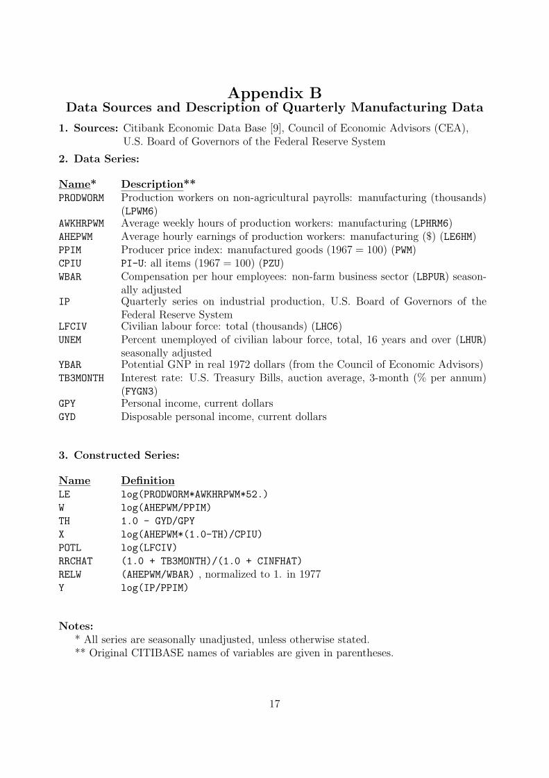
Appendix BData Sources and Description of Quarterly Manufacturing Data

1. Sources: Citibank Economic Data Base [9], Council of Economic Advisors (CEA),U.S. Board of Governors of the Federal Reserve System

2. Data Series:

Name* Description**PRODWORM Production workers on non-agricultural payrolls: manufacturing (thousands)

(LPWM6)AWKHRPWM Average weekly hours of production workers: manufacturing (LPHRM6)AHEPWM Average hourly earnings of production workers: manufacturing ($) (LE6HM)PPIM Producer price index: manufactured goods (1967 = 100) (PWM)CPIU PI-U: all items (1967 = 100) (PZU)WBAR Compensation per hour employees: non-farm business sector (LBPUR) season-

ally adjustedIP Quarterly series on industrial production, U.S. Board of Governors of the

Federal Reserve SystemLFCIV Civilian labour force: total (thousands) (LHC6)UNEM Percent unemployed of civilian labour force, total, 16 years and over (LHUR)

seasonally adjustedYBAR Potential GNP in real 1972 dollars (from the Council of Economic Advisors)TB3MONTH Interest rate: U.S. Treasury Bills, auction average, 3-month (% per annum)

(FYGN3)GPY Personal income, current dollarsGYD Disposable personal income, current dollars

3. Constructed Series:

Name DefinitionLE log(PRODWORM*AWKHRPWM*52.)

W log(AHEPWM/PPIM)

TH 1.0 - GYD/GPY

X log(AHEPWM*(1.0-TH)/CPIU)

POTL log(LFCIV)

RRCHAT (1.0 + TB3MONTH)/(1.0 + CINFHAT)

RELW (AHEPWM/WBAR) , normalized to 1. in 1977Y log(IP/PPIM)

Notes:* All series are seasonally unadjusted, unless otherwise stated.** Original CITIBASE names of variables are given in parentheses.

17

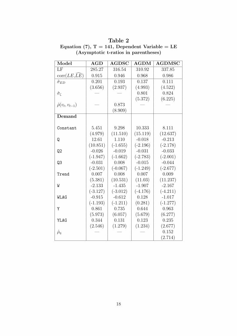
Table 2Equation (7), T = 141, Dependent Variable = LE

(Asymptotic t-ratios in parentheses)

Model AGD AGDSC AGDM AGDMSCLF 285.27 316.54 310.92 337.85

corr(LE,LE) 0.915 0.946 0.968 0.986σED 0.201 0.193 0.137 0.111

(3.656) (2.937) (4.993) (4.522)σζ — — 0.801 0.824

(5.372) (6.225)ρ(vt, vt−1) — 0.873 — —

(8.909)Demand

Constant 5.451 9.298 10.333 8.111(4.979) (11.510) (15.119) (12.637)

Q 12.61 1.110 -0.018 -0.213(10.851) (-1.655) (-2.196) (-2.178)

Q2 -0.026 -0.019 -0.031 -0.033(-1.947) (-1.662) (-2.783) (-2.001)

Q3 -0.031 0.008 -0.015 -0.044(-2.501) (-0.067) (-1.249) (-2.677)

Trend 0.007 0.008 0.007 0.009(5.381) (10.531) (11.03) (11.237)

W -2.133 -1.435 -1.907 -2.167(-3.127) (-3.012) (-4.176) (-4.211)

WLAG -0.915 -0.612 0.128 -1.017(-1.193) (-1.211) (0.281) (-1.277)

Y 0.861 0.735 0.644 0.963(5.973) (6.057) (5.679) (6.277)

YLAG 0.344 0.131 0.123 0.235(2.546) (1.279) (1.234) (2.677)

ρη — — — 0.152(2.714)

18

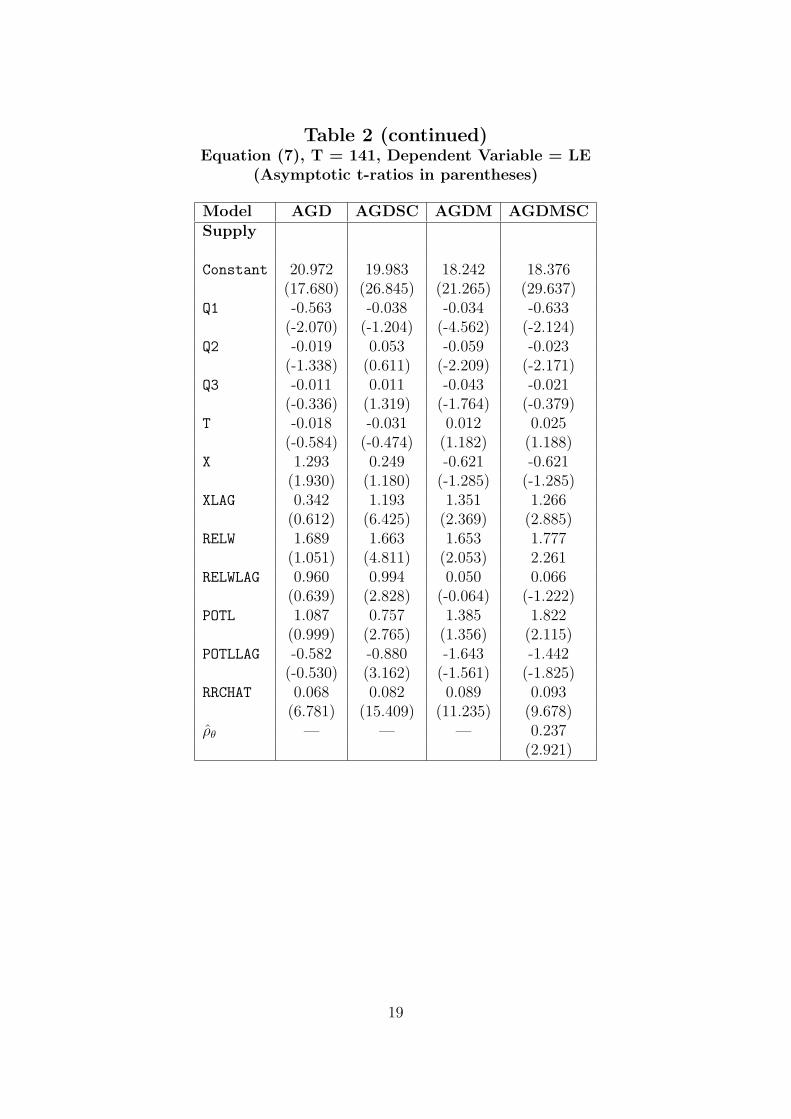
Table 2 (continued)Equation (7), T = 141, Dependent Variable = LE

(Asymptotic t-ratios in parentheses)

Model AGD AGDSC AGDM AGDMSCSupply

Constant 20.972 19.983 18.242 18.376(17.680) (26.845) (21.265) (29.637)

Q1 -0.563 -0.038 -0.034 -0.633(-2.070) (-1.204) (-4.562) (-2.124)

Q2 -0.019 0.053 -0.059 -0.023(-1.338) (0.611) (-2.209) (-2.171)

Q3 -0.011 0.011 -0.043 -0.021(-0.336) (1.319) (-1.764) (-0.379)

T -0.018 -0.031 0.012 0.025(-0.584) (-0.474) (1.182) (1.188)

X 1.293 0.249 -0.621 -0.621(1.930) (1.180) (-1.285) (-1.285)

XLAG 0.342 1.193 1.351 1.266(0.612) (6.425) (2.369) (2.885)

RELW 1.689 1.663 1.653 1.777(1.051) (4.811) (2.053) 2.261

RELWLAG 0.960 0.994 0.050 0.066(0.639) (2.828) (-0.064) (-1.222)

POTL 1.087 0.757 1.385 1.822(0.999) (2.765) (1.356) (2.115)

POTLLAG -0.582 -0.880 -1.643 -1.442(-0.530) (3.162) (-1.561) (-1.825)

RRCHAT 0.068 0.082 0.089 0.093(6.781) (15.409) (11.235) (9.678)

ρθ — — — 0.237(2.921)

19

Table 3Equation (7), T = 141, Dependent Variable = LE

(Asymptotic t-ratios in parentheses)

Model AGD AGDSC AGDM AGDMSCLF 295.36 326.71 323.94 346.43

corr(LE,LE) 0.925 0.951 0.974 0.989σED 0.203 0.187 0.139 0.102

(3.233) (3.031) (5.023) (4.311)σζ — — 0.817 0.837

(5.993) (6.137)ρ(vt, vt−1) — 0.867 (9.121)ρ(LEt, LEt−1) 0.937 0.078 0.193 0.013

(11.236) (0.874) (2.676) (0.637)DemandConstant 5.236 6.407 9.714 10.263

(4.372) (2.071) (14.041) (13.346)Q1 1.182 1.113 -0.027 -0.025

(9.629) (-0.813) (-2.610) (-2.160)Q2 -0.023 -0.016 -0.039 -0.031

(-1.735) (-1.325) (-3.236) (-2.834)Q3 -0.027 -0.024 -0.019 -0.015

(-2.352) (-1.123) (-1.677) (-1.248)Trend 0.006 0.011 0.007 0.007

(4.992) (3.646) (11.566) (9.828)W -2.018 -2.121 -3.758 -1.931

(-3.001) (-2.161) (-4.313) (-4.134)WLAG -0.978 -0.674 -1.815 -0.134

(-1.105) (-0.678) (-2.094) (-0.274)Y 0.872 1.125 1.071 0.652

(5.283) (4.312) (7.328) (5.629)YLAG 0.307 0.009 0.259 0.121

(1.993) (1.374) (1.904) (1.177)WRES 2.769 2.931 3.993 3.762

(3.008) (2.993) (3.054) (2.821)XRES 1.563 1.611 2.036 1.992

(3.372) (3.459) (3.036) (2.731)ρη — — — 0.131

(1.631)

20

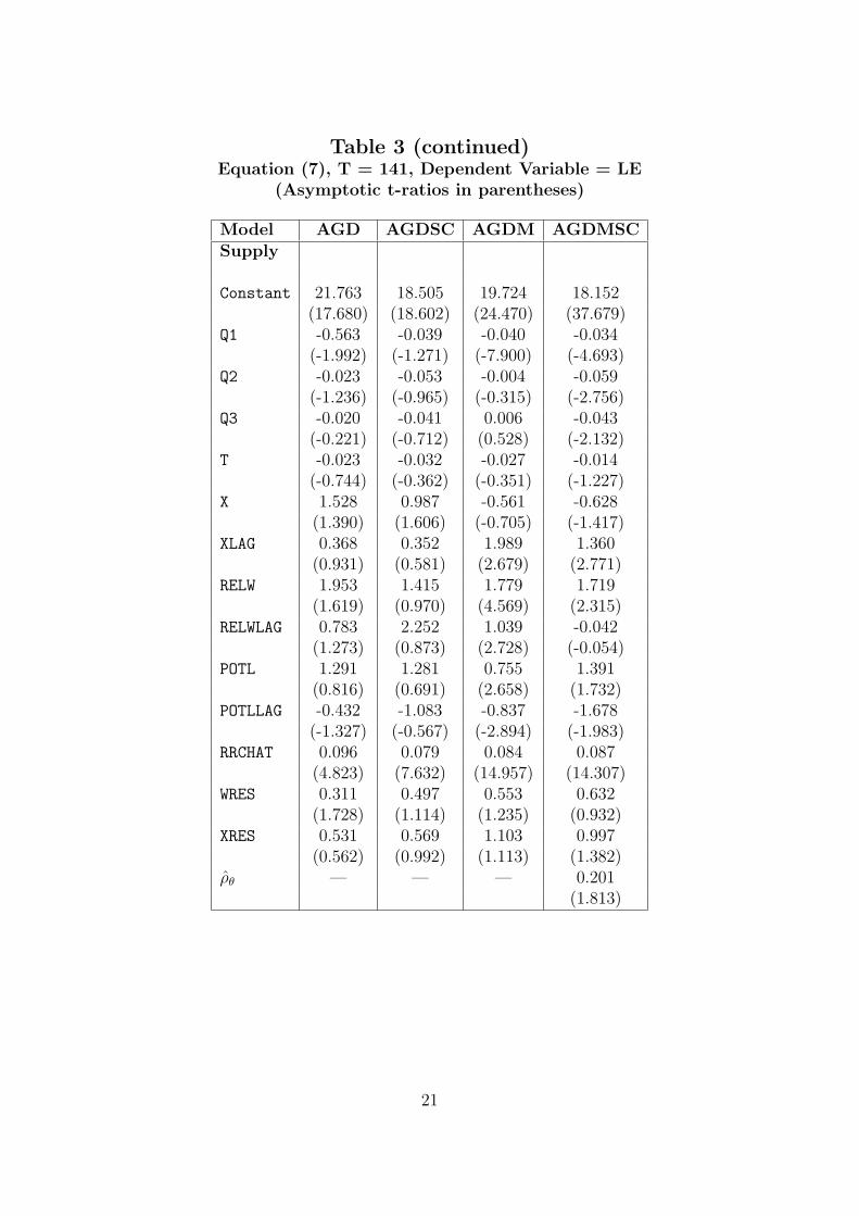
Table 3 (continued)Equation (7), T = 141, Dependent Variable = LE

(Asymptotic t-ratios in parentheses)

Model AGD AGDSC AGDM AGDMSCSupply

Constant 21.763 18.505 19.724 18.152(17.680) (18.602) (24.470) (37.679)

Q1 -0.563 -0.039 -0.040 -0.034(-1.992) (-1.271) (-7.900) (-4.693)

Q2 -0.023 -0.053 -0.004 -0.059(-1.236) (-0.965) (-0.315) (-2.756)

Q3 -0.020 -0.041 0.006 -0.043(-0.221) (-0.712) (0.528) (-2.132)

T -0.023 -0.032 -0.027 -0.014(-0.744) (-0.362) (-0.351) (-1.227)

X 1.528 0.987 -0.561 -0.628(1.390) (1.606) (-0.705) (-1.417)

XLAG 0.368 0.352 1.989 1.360(0.931) (0.581) (2.679) (2.771)

RELW 1.953 1.415 1.779 1.719(1.619) (0.970) (4.569) (2.315)

RELWLAG 0.783 2.252 1.039 -0.042(1.273) (0.873) (2.728) (-0.054)

POTL 1.291 1.281 0.755 1.391(0.816) (0.691) (2.658) (1.732)

POTLLAG -0.432 -1.083 -0.837 -1.678(-1.327) (-0.567) (-2.894) (-1.983)

RRCHAT 0.096 0.079 0.084 0.087(4.823) (7.632) (14.957) (14.307)

WRES 0.311 0.497 0.553 0.632(1.728) (1.114) (1.235) (0.932)

XRES 0.531 0.569 1.103 0.997(0.562) (0.992) (1.113) (1.382)

ρθ — — — 0.201(1.813)

21

References

[1] Altonji, J.G. (1982): “The Intertemporal Substitution Model of Labour Market Fluc-tuations: An Empirical Analysis,” Review of Economic Studies, XLIX.

[2] Altonji, J.G. and O. Ashenfelter (1980): “Wage Movements and the Labour MarketEquilibrium Hypothesis,” Economica, (August).

[3] Andrews, D.W.K. (1989): “An Empirical Process Central Limit Theorem for DependentNon-identically Distributed Random Variables,” Journal of Multivariate Analysis, v.38(August), 187–203.

[4] Andrews, M. and S. Nickell (1986): “A Disaggregated Disequilibrium Model of theLabour Market,” Oxford Economic Papers, v.38, 3 (November).

[5] Barro, R.J. and H.I. Grossman (1971): “A General Disequilibrium Model of Incomeand Employment,” American Economic Review, 61 (March).

[6] Bouissou, M.B., J.J. Laffont and Q.H. Vuong (1986): “Disequilibrium Econometrics onMicro Data,” Review of Economic Studies, LIII.

[7] Box, G.E.P. and G.M. Jenkins (1970): Time Series Analysis, Forecasting and Control.San Francisco, Holden Day.

[8] Butler, J. and R. Moffit (1982): “A Computationally Efficient Quadrature Procedurefor the One-Factor Multinomial Probit Model,” Econometrica 50.

[9] CITIBASE: Citibank Economic Database, New York, Citibank. 1986 Update.

[10] Eaton, J. and R. Quandt: (1983): “A Quasi-Walrasian Model of Rationing and LaborSupply,” Economica (August).

[11] Engle, R. Hendry, D.F. and J.F. Richard (1983): “Exogeneity,” Econometrica, January.

[12] Fair, R.C. and D.M. Jaffee (1972): “Methods of Estimation for Markets in Disequilib-rium,” Econometrica, 40 (May).

[13] Goldfeld, S.M. and R.D. Quandt (1975): “Estimation of a Disequilibrium Model andthe Value of Information,” Journal of Econometrics, 3.

[14] Gourieroux, C., A. Monfort, and A. Trognon (1984): “Pseudo Maximum LikelihoodMethods: Theory,” Econometrica, 52, 681–700.

[15] Hajivassiliou, V.A. (1984): “A Computationally Efficient Quadrature Method for theOne-Factor Multinomial Probit Model,” MIT mimeo.

[16] Hajivassiliou, V.A. (1985): “Disequilibrium and Other Limited Dependent VariablesModels in Econometrics,” unpublished Ph.D. thesis, Massachusetts Institute of Tech-nology.

22

[17] Hajivassiliou, V.A. (1986): “Two Misspecification Tests for the Simple Switching Re-gressions Disequilibrium Model,” Economics Letters, 22.

[18] Hajivassiliou, V.A. (1987): “An Aggregative Disequilibrium Model of the US LabourMarket,” Cowles Foundation Discussion Paper # 848, Yale University.

[19] Hansen, L.P. and Singleton (1982): “Generalized Instrumental Variables Estimation ofNonlinear Rational Expectations Models,” Econometrica, 50 (September).

[20] Kooiman, P. (1984): “Smoothing the Aggregate Fix-price Model and the Use of BusinessSurvey Data,” The Economic Journal, December.

[21] Laffont, J.J. and A. Monfort (1979): “Disequilibrium Econometrics in Dynamic Mod-els,” Journal of Econometrics, 11.

[22] Lambert, J.P. (1984): “Models Macro-Economique de Rationnement et Enquettes deConjoctures,” Les Recherches Economiques de Louvain: Louvain-La-Neuve, Belgium.

[23] Laroque, G. and B. Salanie (1989). “Estimation of Multi-Market Disequilibrium Fix-Price Models: An Application of Pseudo Maximum Likelihood Methods,” Econometrica,bf 57, 831-860.

[24] Laroque, G. and B. Salanie (1992). “Simulation Estimation of Disequilibrium Modelswith Serial Correlation: Theoretical and Monte Carlo Results,” INSEE mimeo, pre-sented at International Conference on Simulation, Rotterdam, The Netherlands.

[25] Lee, L.-F. (1984): “The Likelihood Function and a Test for Serial Correlation in aDisequilibrium Market Model,” Economics Letters, V. 14, Nos. 2-3.

[26] Maddala, G. and F. Nelson (1974): “Maximum Likelihood Methods for Markets inDisequilibrium,” Econometrica, 42.

[27] Malinvaud, E. (1980): “Macroeconomic Rationing of Employment,” in E. Malinvaudand J.P. Fitoussi, Unemployment in Western Countries, London, MacMillan.

[28] Mankiw, N.G., J. Rotemberg and L. Summers (1985): “The Intertemporal Hypothesisin Macroeconomics,” Quarterly Journal of Economics (February).

[29] McFadden, D. (1989). “A Method of Simulated Moments for Estimation of DiscreteResponse Models without Numerical Integration,” Econometrica 57, 995-1026.

[30] Muellbauer, J. (1978): “Macro Theory vs. Macro Econometrics: The Treatment ofDisequilibrium in Macro Models,” Birkbeck College Discussion Paper, 79 (April).

[31] Newey, W. and K. West (1987): “A Simple, Positive Definite, Heteroskedasticity andAutocorrelation Consistent Covariance Matrix,” Econometrica.

[32] Pakes, A. and D. Pollard (1989). “Simulation and the Asymptotics of OptimizationEstimators,” Econometrica 57, 1027-1057.

23

[33] Quandt, R.E. (1981): “Autocorrelated Errors in Simple Disequilibrium Models,” Eco-nomics Letters, 7.

[34] Quandt, R.E. (1982): “Econometric Disequilibrium Models,” Econometric Reviews, 1.

[35] Quandt, R.E. (1986): “Estimation in Disequilibrium Models with Aggregation,” Finan-cial Research Center Memorandum No. 68, Princeton University.

[36] Quandt, R. and H. Rosen (1986): “Unemployment, Disequilibrium and the Short-RunPhillips Curve: An Econometric Approach,” Journal of Applied Econometrics, Vol.1,235-253.

[37] Richard, J.-F. (1992): “An Acceleration Method for Simulation Estimation of DynamicLimited Dependent Variable Models,” mimeo, University of Pittsburgh.

[38] Robinson, P. (1982): “On the Asymptotic Properties of Models Containing LimitedDependent Variables,” Econometrica (January).

[39] Romer, D. (1981): “Rosen and Quandt’s Disequilibrium Model of the Labor Market: ARevision,” Review of Economics and Statistics.

[40] Rosen, H.S. and R.E. Quandt (1978): “Estimation of a Disequilibrium Aggregate LaborMarket,” Review of Economics and Statistics, 60.

[41] Salanie, B. (1989): “Wage and Price Adjustment in a Multimarket DisequilibriumModel,” Journal of Applied Econometrics.

[42] Sargent, T.J. (1978): “Estimation of Dynamic Labour Demand Schedules Under Ratio-nal Expectations,” Journal of Political Economy (December).

24