Aggressive Quadrotor Flight through Cluttered Environments Using

Mixed Integer Programming

Benoit Landry1, Robin Deits1, Peter R. Florence1 and Russ Tedrake1

Abstract— Quadrotor flight has typically been limited tosparse environments due to numerical complications that arisewhen dealing with large numbers of obstacles. We hypothesizedthat it would be possible to plan and robustly execute trajecto-ries in obstacle-dense environments using the novel IterativeRegional Inflation by Semidefinite programming algorithm(IRIS), mixed-integer semidefinite programs (MISDP), and amodel-based controller. Unlike sampling-based approaches, thealgorithm guarantees non-penetration of the trajectories evenwith small obstacles such as strings. We present experimentalvalidation of this hypothesis by aggressively flying a smallquadrotor (34g, 92mm rotor to rotor) in a series of indoorenvironments including a cubic meter volume containing 20interwoven strings.

I. INTRODUCTION

Advances in research have brought the quadrotor to a

level of sophistication that is making it increasingly attractive

for a variety of commercial applications like surveying and

delivery. In order for these applications to become a reality,

we now need algorithms that can deal reliably with environ-

ments that are substantially more cluttered than a laboratory

setting. The most successful algorithms put forward to enable

quadrotors to avoid obstacles often require an exponential

increase in planning time with respect to the number of

obstacles by, for example, introducing an integer variable

for each face of obstacles in the environment. Most of these

algorithms therefore start to perform poorly as the number

of obstacles is increased beyond a modest handful of them

[1] [2].

Recently, it has been suggested that the challenges of

increasing obstacle density may be overcome by the novel

Iterative Regional Inflation by semidifinite programming

algorithm (IRIS) that segments space into obstacle-free

regions. Planning paths through this segmentation can be

accomplished using mixed-integer convex optimization, with

the complexity growing with the much more manageable

number of free-space segments instead of the number of

obstacle faces. Hence, it can produce trajectories in environ-

ments containing many more obstacles than was previously

demonstrated. Moreover the non-penetration constraint that

the algorithm enforces along the entire path promise better

performance with small obstacles than previous approaches

that rely on sampling. We hypothesized that it would be

possible to aggressively fly a small quadrotor through en-

vironments containing greater number of obstacles than

ever demonstrated before by leveraging IRIS, MISDPs, and

The authors are with (1) Computer Science and ArtificialIntelligence Laboratory, MIT, Cambridge, MA 02139, USA{landry,rdeits,peteflo,russt}@mit.edu

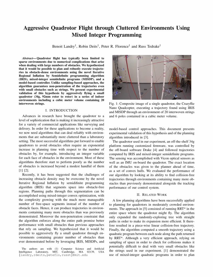
Fig. 1: Composite image of a single quadrotor, the Crazyflie

Nano Quadcopter, executing a trajectory found using IRIS

and MISDP through an environment of 20 interwoven strings

and 6 poles contained in a cubic meter volume.

model-based control approaches. This document presents

experimental validation of this hypothesis and of the planning

algorithm introduced in [3].

The quadrotor used in our experiment, an off-the-shelf 34g

platform running customized firmware, was controlled by

the off-board software Drake [4] and followed trajectories

computed by IRIS and mixed-integer semidefinite programs.

The sensing was accomplished with Vicon optical sensors as

well as an IMU on-board the quadrotor. The exact location

of the obstacles was given to the planner ahead of time,

as a set of convex hulls. We evaluated the performance of

our algorithm by looking at its ability to find collision-free

trajectories through environments containing many more ob-

stacles than previously demonstrated alongside the tracking

performance of our control system.

II. RELATED WORK

A few planning algorithms have been successfully applied

to planning for quadrotors in moderately crowded environ-

ments. The approach in [5] consisted of running RRT* in the

entire space where the quadrotor might fly. The algorithm

only expanded the randomly-exploring tree with straight

paths in order to make its expansion more efficient. It there-

fore resulted in a piece-wise linear collision-free trajectory.

Finally, the algorithm computed a smooth trajectory using a

quadratic program between each node along the path returned

by RRT*. Although a very efficient approach, relying on

sampling of space in order to check for collisions makes it

potentially difficult to deal with very small obstacles like

the strings used in our experiment. [1] demonstrated the

use of mixed-integer quadratic programs in order to plan

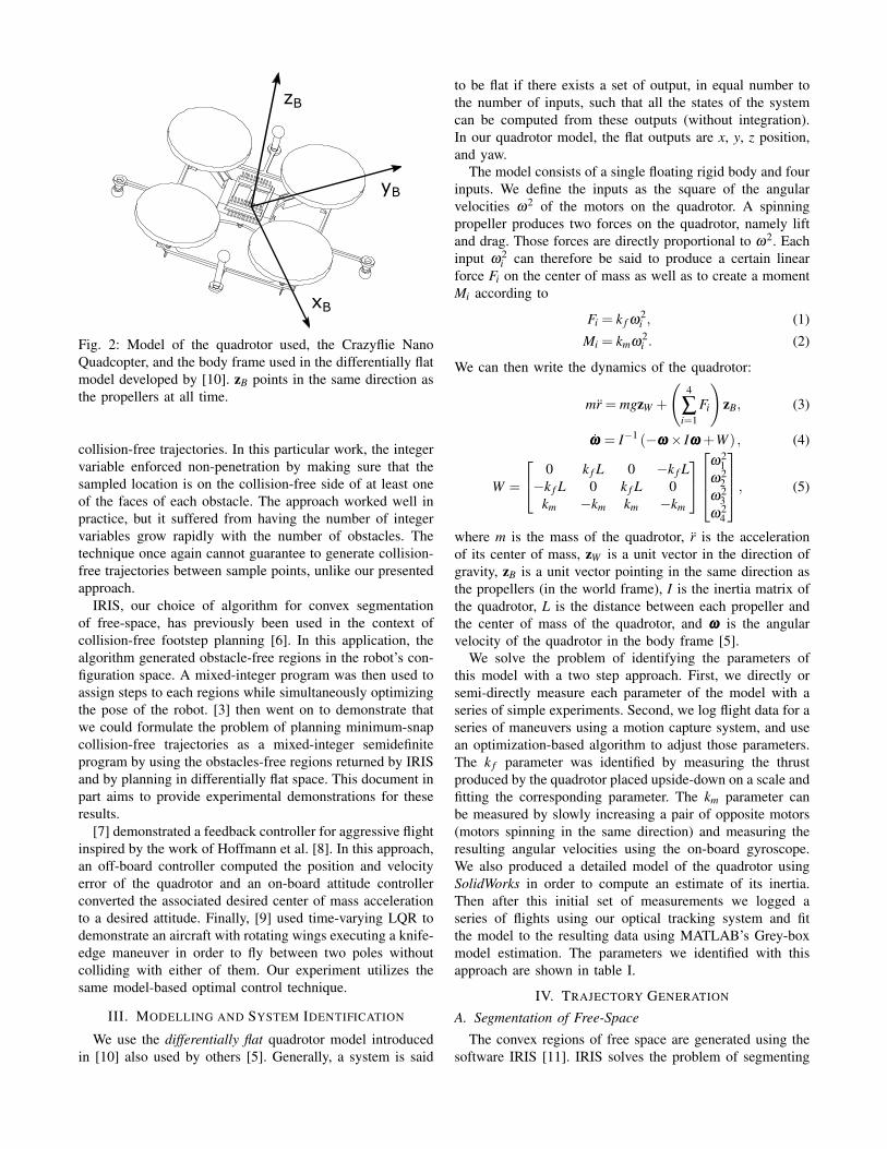
Fig. 2: Model of the quadrotor used, the Crazyflie Nano

Quadcopter, and the body frame used in the differentially flat

model developed by [10]. zB points in the same direction as

the propellers at all time.

collision-free trajectories. In this particular work, the integer

variable enforced non-penetration by making sure that the

sampled location is on the collision-free side of at least one

of the faces of each obstacle. The approach worked well in

practice, but it suffered from having the number of integer

variables grow rapidly with the number of obstacles. The

technique once again cannot guarantee to generate collision-

free trajectories between sample points, unlike our presented

approach.

IRIS, our choice of algorithm for convex segmentation

of free-space, has previously been used in the context of

collision-free footstep planning [6]. In this application, the

algorithm generated obstacle-free regions in the robot’s con-

figuration space. A mixed-integer program was then used to

assign steps to each regions while simultaneously optimizing

the pose of the robot. [3] then went on to demonstrate that

we could formulate the problem of planning minimum-snap

collision-free trajectories as a mixed-integer semidefinite

program by using the obstacles-free regions returned by IRIS

and by planning in differentially flat space. This document in

part aims to provide experimental demonstrations for these

results.

[7] demonstrated a feedback controller for aggressive flight

inspired by the work of Hoffmann et al. [8]. In this approach,

an off-board controller computed the position and velocity

error of the quadrotor and an on-board attitude controller

converted the associated desired center of mass acceleration

to a desired attitude. Finally, [9] used time-varying LQR to

demonstrate an aircraft with rotating wings executing a knife-

edge maneuver in order to fly between two poles without

colliding with either of them. Our experiment utilizes the

same model-based optimal control technique.

III. MODELLING AND SYSTEM IDENTIFICATION

We use the differentially flat quadrotor model introduced

in [10] also used by others [5]. Generally, a system is said

to be flat if there exists a set of output, in equal number to

the number of inputs, such that all the states of the system

can be computed from these outputs (without integration).

In our quadrotor model, the flat outputs are x, y, z position,

and yaw.

The model consists of a single floating rigid body and four

inputs. We define the inputs as the square of the angular

velocities ω2 of the motors on the quadrotor. A spinning

propeller produces two forces on the quadrotor, namely lift

and drag. Those forces are directly proportional to ω2. Each

input ω2i can therefore be said to produce a certain linear

force Fi on the center of mass as well as to create a moment

Mi according to

Fi = k f ω2i , (1)

Mi = kmω2i . (2)

We can then write the dynamics of the quadrotor:

mr = mgzW +

(

4

∑i=1

Fi

)

zB, (3)

ωωω = I−1 (−ωωω × Iωωω +W ) , (4)

W =

0 k f L 0 −k f L

−k f L 0 k f L 0

km −km km −km

ω21

ω22

ω23

ω24

, (5)

where m is the mass of the quadrotor, r is the acceleration

of its center of mass, zW is a unit vector in the direction of

gravity, zB is a unit vector pointing in the same direction as

the propellers (in the world frame), I is the inertia matrix of

the quadrotor, L is the distance between each propeller and

the center of mass of the quadrotor, and ωωω is the angular

velocity of the quadrotor in the body frame [5].

We solve the problem of identifying the parameters of

this model with a two step approach. First, we directly or

semi-directly measure each parameter of the model with a

series of simple experiments. Second, we log flight data for a

series of maneuvers using a motion capture system, and use

an optimization-based algorithm to adjust those parameters.

The k f parameter was identified by measuring the thrust

produced by the quadrotor placed upside-down on a scale and

fitting the corresponding parameter. The km parameter can

be measured by slowly increasing a pair of opposite motors

(motors spinning in the same direction) and measuring the

resulting angular velocities using the on-board gyroscope.

We also produced a detailed model of the quadrotor using

SolidWorks in order to compute an estimate of its inertia.

Then after this initial set of measurements we logged a

series of flights using our optical tracking system and fit

the model to the resulting data using MATLAB’s Grey-box

model estimation. The parameters we identified with this

approach are shown in table I.

IV. TRAJECTORY GENERATION

A. Segmentation of Free-Space

The convex regions of free space are generated using the

software IRIS [11]. IRIS solves the problem of segmenting

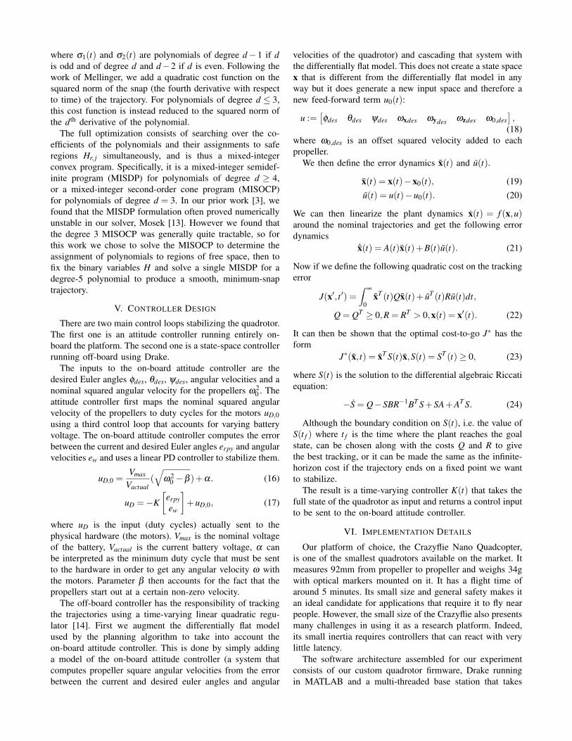
Parameter Value

Ixx 2.3951 ·10−5kg ·m2

Iyy 2.3951 ·10−5kg ·m2

Izz 3.2347 ·10−5kg ·m2

Km 1.8580 ·10−5N ·m · s2

K f 0.005022N · s2

TABLE I: Parameters of our model of the Crazyflie Nano

Quadcopter

3D space into a set of convex regions through a series of

convex optimizations. More specifically, IRIS alternates be-

tween two optimizations. The first optimization is a quadratic

program that finds hyperplanes that separate a convex region

of space from the obstacles. The second optimization is

a semidefinite program that takes the intersection of those

hyperplanes, and finds an ellipsoid of maximum volume

inscribed inside those hyperplanes.

In order to account for the dimensions of the quadrotor,

we inflate the convex hulls representing the obstacles before

passing them to IRIS. We inflate the obstacles by moving

each one of their planes in the direction of their normal by

an amount equal to the radius of the quadrotor. This allows

us to treat the quadrotor as a dimensionless object for the

rest of the planning.

B. Mixed Integer Semidefinite Program

Ordinarily, designing a trajectory for a dynamical system

such as a quadrotor would require us to consider the full state

of our model (in this case, the position, velocity, orientation,

and angular velocity of the center of mass) and its inputs. The

model of the quadrotor used in this work, however, has the

attractive quality of being differentially flat in four outputs,

namely the x, y, and z position and yaw of the model’s center

of mass [10]. From a trajectory in those four flat outputs, we

can derive a trajectory of the entire state of the model and

its inputs by following the procedure described in [10]. We

further simplify the problem by setting the yaw trajectory to

zero during the optimization.

We follow the procedure described in [3] to represent

trajectories in x, y, z as piecewise polynomial functions of

time, and we fix the timespan of each polynomial piece to

an arbitrary range of 0 to 1. This arbitrary timespan can

be adjusted after the optimization to control the actual time

spent executing the trajectory. With the timespan fixed, the

trajectory optimization consists of choosing the coefficients

of the piecewise polynomials. Additionally, we constrain that

the piecewise polynomial be continuous up to the (d −1)th

derivative, where d is the degree of each polynomial piece.

In order to ensure that the trajectories generated are fully

collision-free, we require that each polynomial piece be fully

contained within some convex region of obstacle-free space.

This is a conservative approach, since it is entirely possible

for a trajectory to be collision-free without having each

polynomial lie within a single convex volume, but it is an

advantageous constraint because it converts our problem into

one we can efficiently solve to its global optimum.

We represent the assignment of polynomial pieces to con-

vex regions of free space with a matrix of binary variables,

H ∈ {0,1}R×N, where R is the number of convex regions and

N is the number of polynomial trajectory pieces. For each

element of H, we constrain that if Hr, j = 1, then polynomial

j must be contained within region r. This constraint can

be represented as a combination of linear and semidefinite

constraints for a polynomial of arbitrary degree, although

it can be reduced to a second-order cone constraint for

polynomials of degree 3 [3].

To ensure that every polynomial is contained in some

convex region, we add linear constraints of the form:

R

∑r=1

Hr, j = 1 ∀ j ∈ 1, . . . ,N, (6)

[12] showed that sum of squares constraints can be formu-

lated as semidefinite programs. We therefore formulate our

non-penetration constraint as a sum of squares constraint.

First we define the polynomial j as a linear combination of

polynomial basis functions φ1(t), ...,φd+1(t).

Pj(t) =d+1

∑k=1

C j,kφk(t) t ∈ [0,1], (7)

Therefore if Hr, j is set to 1, then the polynomial must be

contained inside the safe region r

ArPj(t)≤ br ∀t ∈ [0,1], (8)

or

Ar

d+1

∑k=1

C j,kφk(t)≤ br ∀t ∈ [0,1]. (9)

The constraint 9 can be written as m constraints of the form

aTr,l

d+1

∑k=1

C j,kφk(t)≤ br,l ∀t ∈ [0,1], (10)

where

Ar =

aTr,1

aTr,2

...

aTr,m

and b =

br,1

br,2

...

br,m

. (11)

By redistributing the terms in 10, we get:

d+1

∑k=1

(aTr,lC j,k)φk(t)≤ br,l ∀t ∈ [0,1], (12)

with which we can now define q(t)

q(t) := br,l −d+1

∑k=1

(aTr,lC j,k)φk(t)≥ 0 ∀t ∈ [0,1]. (13)

The polynomial Pj(t) is fully contained in region r if and

only if q(t)≥ 0∀t ∈ [0,1]. This holds if and only if q(t) can

be written as:

q(t) =

{

tσ1(t)+(1− t)σ2(t) if d is odd

σ1(t)+ t(1− t)σ2(t) if d is even(14)

σ1(t),σ2(t) are sums of squares (15)

where σ1(t) and σ2(t) are polynomials of degree d −1 if d

is odd and of degree d and d−2 if d is even. Following the

work of Mellinger, we add a quadratic cost function on the

squared norm of the snap (the fourth derivative with respect

to time) of the trajectory. For polynomials of degree d ≤ 3,

this cost function is instead reduced to the squared norm of

the dth derivative of the polynomial.

The full optimization consists of searching over the co-

efficients of the polynomials and their assignments to safe

regions Hr, j simultaneously, and is thus a mixed-integer

convex program. Specifically, it is a mixed-integer semidef-

inite program (MISDP) for polynomials of degree d ≥ 4,

or a mixed-integer second-order cone program (MISOCP)

for polynomials of degree d = 3. In our prior work [3], we

found that the MISDP formulation often proved numerically

unstable in our solver, Mosek [13]. However we found that

the degree 3 MISOCP was generally quite tractable, so for

this work we chose to solve the MISOCP to determine the

assignment of polynomials to regions of free space, then to

fix the binary variables H and solve a single MISDP for a

degree-5 polynomial to produce a smooth, minimum-snap

trajectory.

V. CONTROLLER DESIGN

There are two main control loops stabilizing the quadrotor.

The first one is an attitude controller running entirely on-

board the platform. The second one is a state-space controller

running off-board using Drake.

The inputs to the on-board attitude controller are the

desired Euler angles φdes, θdes, ψdes, angular velocities and a

nominal squared angular velocity for the propellers ω20 . The

attitude controller first maps the nominal squared angular

velocity of the propellers to duty cycles for the motors uD,0

using a third control loop that accounts for varying battery

voltage. The on-board attitude controller computes the error

between the current and desired Euler angles erpy and angular

velocities ew and uses a linear PD controller to stabilize them.

uD,0 =Vmax

Vactual

(√

ω20 −β )+α. (16)

uD =−K

[

erpy

ew

]

+uD,0, (17)

where uD is the input (duty cycles) actually sent to the

physical hardware (the motors). Vmax is the nominal voltage

of the battery, Vactual is the current battery voltage, α can

be interpreted as the minimum duty cycle that must be sent

to the hardware in order to get any angular velocity ω with

the motors. Parameter β then accounts for the fact that the

propellers start out at a certain non-zero velocity.

The off-board controller has the responsibility of tracking

the trajectories using a time-varying linear quadratic regu-

lator [14]. First we augment the differentially flat model

used by the planning algorithm to take into account the

on-board attitude controller. This is done by simply adding

a model of the on-board attitude controller (a system that

computes propeller square angular velocities from the error

between the current and desired euler angles and angular

velocities of the quadrotor) and cascading that system with

the differentially flat model. This does not create a state space

x that is different from the differentially flat model in any

way but it does generate a new input space and therefore a

new feed-forward term u0(t):

u :=[

φdes θdes ψdes ωxdes ωydesωzdes ω0,des

]

,

(18)

where ω0,des is an offset squared velocity added to each

propeller.

We then define the error dynamics x(t) and u(t).

x(t) = x(t)−x0(t), (19)

u(t) = u(t)−u0(t). (20)

We can then linearize the plant dynamics x(t) = f (x,u)around the nominal trajectories and get the following error

dynamics˙x(t) = A(t)x(t)+B(t)u(t). (21)

Now if we define the following quadratic cost on the tracking

error

J(x′, t ′) =∫ ∞

0xT (t)Qx(t)+ uT (t)Ru(t)dt,

Q = QT ≥ 0,R = RT> 0,x(t) = x′(t). (22)

It can then be shown that the optimal cost-to-go J∗ has the

form

J∗(x, t) = xT S(t)x,S(t) = ST (t)≥ 0, (23)

where S(t) is the solution to the differential algebraic Riccati

equation:

−S = Q−SBR−1BT S+SA+AT S. (24)

Although the boundary condition on S(t), i.e. the value of

S(t f ) where t f is the time where the plant reaches the goal

state, can be chosen along with the costs Q and R to give

the best tracking, or it can be made the same as the infinite-

horizon cost if the trajectory ends on a fixed point we want

to stabilize.

The result is a time-varying controller K(t) that takes the

full state of the quadrotor as input and returns a control input

to be sent to the on-board attitude controller.

VI. IMPLEMENTATION DETAILS

Our platform of choice, the Crazyflie Nano Quadcopter,

is one of the smallest quadrotors available on the market. It

measures 92mm from propeller to propeller and weighs 34g

with optical markers mounted on it. It has a flight time of

around 5 minutes. Its small size and general safety makes it

an ideal candidate for applications that require it to fly near

people. However, the small size of the Crazyflie also presents

many challenges in using it as a research platform. Indeed,

its small inertia requires controllers that can react with very

little latency.

The software architecture assembled for our experiment

consists of our custom quadrotor firmware, Drake running

in MATLAB and a multi-threaded base station that takes

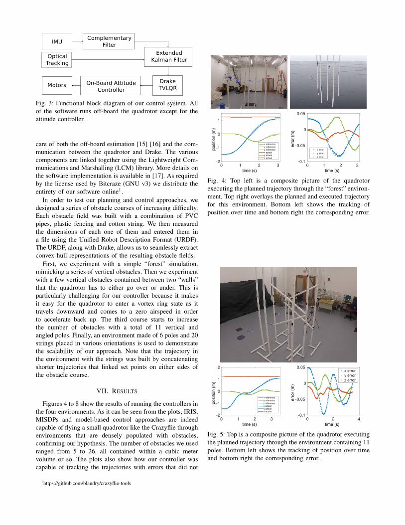
Fig. 3: Functional block diagram of our control system. All

of the software runs off-board the quadrotor except for the

attitude controller.

care of both the off-board estimation [15] [16] and the com-

munication between the quadrotor and Drake. The various

components are linked together using the Lightweight Com-

munications and Marshalling (LCM) library. More details on

the software implementation is available in [17]. As required

by the license used by Bitcraze (GNU v3) we distribute the

entirety of our software online1.

In order to test our planning and control approaches, we

designed a series of obstacle courses of increasing difficulty.

Each obstacle field was built with a combination of PVC

pipes, plastic fencing and cotton string. We then measured

the dimensions of each one of them and entered them in

a file using the Unified Robot Description Format (URDF).

The URDF, along with Drake, allows us to seamlessly extract

convex hull representations of the resulting obstacle fields.

First, we experiment with a simple “forest” simulation,

mimicking a series of vertical obstacles. Then we experiment

with a few vertical obstacles contained between two “walls”

that the quadrotor has to either go over or under. This is

particularly challenging for our controller because it makes

it easy for the quadrotor to enter a vortex ring state as it

travels downward and comes to a zero airspeed in order

to accelerate back up. The third course starts to increase

the number of obstacles with a total of 11 vertical and

angled poles. Finally, an environment made of 6 poles and 20

strings placed in various orientations is used to demonstrate

the scalability of our approach. Note that the trajectory in

the environment with the strings was built by concatenating

shorter trajectories that linked set points on either sides of

the obstacle course.

VII. RESULTS

Figures 4 to 8 show the results of running the controllers in

the four environments. As it can be seen from the plots, IRIS,

MISDPs and model-based control approaches are indeed

capable of flying a small quadrotor like the Crazyflie through

environments that are densely populated with obstacles,

confirming our hypothesis. The number of obstacles we used

ranged from 5 to 26, all contained within a cubic meter

volume or so. The plots also show how our controller was

capable of tracking the trajectories with errors that did not

1https://github.com/blandry/crazyflie-tools

time (s)

0 1 2 3

positio

n (

m)

-2

-1

0

1

x reference

y reference

z reference

x actual

y actual

z actual

time (s)

0 1 2 3

err

or

(m)

-0.1

-0.05

0

0.05

x error

y error

z error

Fig. 4: Top left is a composite picture of the quadrotor

executing the planned trajectory through the “forest” environ-

ment. Top right overlays the planned and executed trajectory

for this environment. Bottom left shows the tracking of

position over time and bottom right the corresponding error.

time (s)

0 1 2 3

positio

n (

m)

-2

-1

0

1

2

x reference

y reference

z reference

x actual

y actual

z actual

time (s)

0 2 4

err

or

(m)

-0.1

-0.05

0

0.05x error

y error

z error

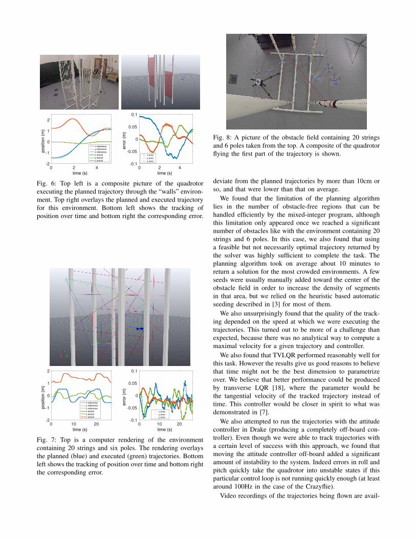
Fig. 5: Top is a composite picture of the quadrotor executing

the planned trajectory through the environment containing 11

poles. Bottom left shows the tracking of position over time

and bottom right the corresponding error.

time (s)

0 2 4

positio

n (

m)

-2

-1

0

1

2

x reference

y reference

z reference

x actual

y actual

z actual

time (s)

0 2 4

err

or

(m)

-0.1

-0.05

0

0.05

0.1

x error

y error

z error

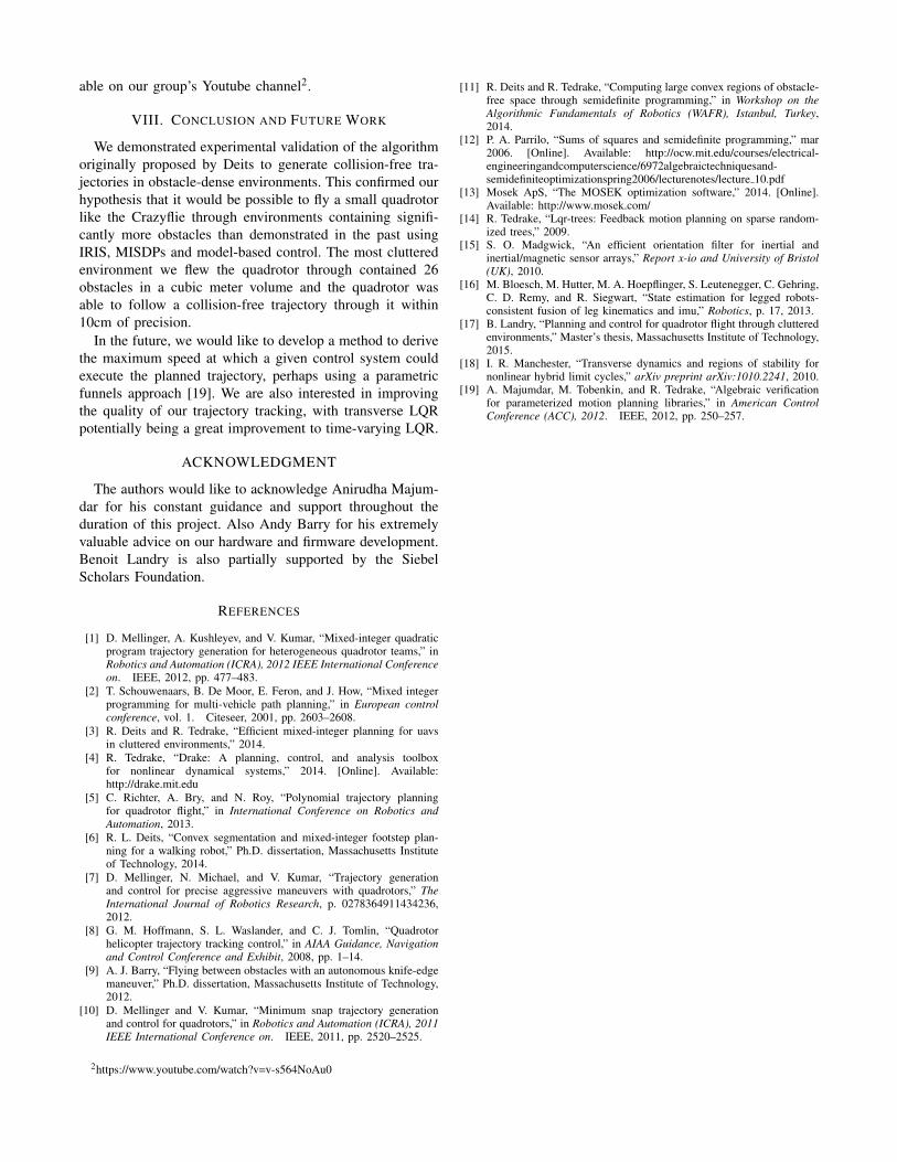
Fig. 6: Top left is a composite picture of the quadrotor

executing the planned trajectory through the “walls” environ-

ment. Top right overlays the planned and executed trajectory

for this environment. Bottom left shows the tracking of

position over time and bottom right the corresponding error.

time (s)

0 10 20

positio

n (

m)

-2

-1

0

1

2

x reference

y reference

z reference

x actual

y actual

z actual

time (s)

0 10 20

err

or

(m)

-0.1

-0.05

0

0.05

0.1

x error

y error

z error

Fig. 7: Top is a computer rendering of the environment

containing 20 strings and six poles. The rendering overlays

the planned (blue) and executed (green) trajectories. Bottom

left shows the tracking of position over time and bottom right

the corresponding error.

Fig. 8: A picture of the obstacle field containing 20 strings

and 6 poles taken from the top. A composite of the quadrotor

flying the first part of the trajectory is shown.

deviate from the planned trajectories by more than 10cm or

so, and that were lower than that on average.

We found that the limitation of the planning algorithm

lies in the number of obstacle-free regions that can be

handled efficiently by the mixed-integer program, although

this limitation only appeared once we reached a significant

number of obstacles like with the environment containing 20

strings and 6 poles. In this case, we also found that using

a feasible but not necessarily optimal trajectory returned by

the solver was highly sufficient to complete the task. The

planning algorithm took on average about 10 minutes to

return a solution for the most crowded environments. A few

seeds were usually manually added toward the center of the

obstacle field in order to increase the density of segments

in that area, but we relied on the heuristic based automatic

seeding described in [3] for most of them.

We also unsurprisingly found that the quality of the track-

ing depended on the speed at which we were executing the

trajectories. This turned out to be more of a challenge than

expected, because there was no analytical way to compute a

maximal velocity for a given trajectory and controller.

We also found that TVLQR performed reasonably well for

this task. However the results give us good reasons to believe

that time might not be the best dimension to parametrize

over. We believe that better performance could be produced

by transverse LQR [18], where the parameter would be

the tangential velocity of the tracked trajectory instead of

time. This controller would be closer in spirit to what was

demonstrated in [7].

We also attempted to run the trajectories with the attitude

controller in Drake (producing a completely off-board con-

troller). Even though we were able to track trajectories with

a certain level of success with this approach, we found that

moving the attitude controller off-board added a significant

amount of instability to the system. Indeed errors in roll and

pitch quickly take the quadrotor into unstable states if this

particular control loop is not running quickly enough (at least

around 100Hz in the case of the Crazyflie).

Video recordings of the trajectories being flown are avail-

able on our group’s Youtube channel2.

VIII. CONCLUSION AND FUTURE WORK

We demonstrated experimental validation of the algorithm

originally proposed by Deits to generate collision-free tra-

jectories in obstacle-dense environments. This confirmed our

hypothesis that it would be possible to fly a small quadrotor

like the Crazyflie through environments containing signifi-

cantly more obstacles than demonstrated in the past using

IRIS, MISDPs and model-based control. The most cluttered

environment we flew the quadrotor through contained 26

obstacles in a cubic meter volume and the quadrotor was

able to follow a collision-free trajectory through it within

10cm of precision.

In the future, we would like to develop a method to derive

the maximum speed at which a given control system could

execute the planned trajectory, perhaps using a parametric

funnels approach [19]. We are also interested in improving

the quality of our trajectory tracking, with transverse LQR

potentially being a great improvement to time-varying LQR.

ACKNOWLEDGMENT

The authors would like to acknowledge Anirudha Majum-

dar for his constant guidance and support throughout the

duration of this project. Also Andy Barry for his extremely

valuable advice on our hardware and firmware development.

Benoit Landry is also partially supported by the Siebel

Scholars Foundation.

REFERENCES

[1] D. Mellinger, A. Kushleyev, and V. Kumar, “Mixed-integer quadraticprogram trajectory generation for heterogeneous quadrotor teams,” inRobotics and Automation (ICRA), 2012 IEEE International Conference

on. IEEE, 2012, pp. 477–483.

[2] T. Schouwenaars, B. De Moor, E. Feron, and J. How, “Mixed integerprogramming for multi-vehicle path planning,” in European control

conference, vol. 1. Citeseer, 2001, pp. 2603–2608.

[3] R. Deits and R. Tedrake, “Efficient mixed-integer planning for uavsin cluttered environments,” 2014.

[4] R. Tedrake, “Drake: A planning, control, and analysis toolboxfor nonlinear dynamical systems,” 2014. [Online]. Available:http://drake.mit.edu

[5] C. Richter, A. Bry, and N. Roy, “Polynomial trajectory planningfor quadrotor flight,” in International Conference on Robotics and

Automation, 2013.

[6] R. L. Deits, “Convex segmentation and mixed-integer footstep plan-ning for a walking robot,” Ph.D. dissertation, Massachusetts Instituteof Technology, 2014.

[7] D. Mellinger, N. Michael, and V. Kumar, “Trajectory generationand control for precise aggressive maneuvers with quadrotors,” The

International Journal of Robotics Research, p. 0278364911434236,2012.

[8] G. M. Hoffmann, S. L. Waslander, and C. J. Tomlin, “Quadrotorhelicopter trajectory tracking control,” in AIAA Guidance, Navigation

and Control Conference and Exhibit, 2008, pp. 1–14.

[9] A. J. Barry, “Flying between obstacles with an autonomous knife-edgemaneuver,” Ph.D. dissertation, Massachusetts Institute of Technology,2012.

[10] D. Mellinger and V. Kumar, “Minimum snap trajectory generationand control for quadrotors,” in Robotics and Automation (ICRA), 2011

IEEE International Conference on. IEEE, 2011, pp. 2520–2525.

2https://www.youtube.com/watch?v=v-s564NoAu0

[11] R. Deits and R. Tedrake, “Computing large convex regions of obstacle-free space through semidefinite programming,” in Workshop on the

Algorithmic Fundamentals of Robotics (WAFR), Istanbul, Turkey,2014.

[12] P. A. Parrilo, “Sums of squares and semidefinite programming,” mar2006. [Online]. Available: http://ocw.mit.edu/courses/electrical-engineeringandcomputerscience/6972algebraictechniquesand-semidefiniteoptimizationspring2006/lecturenotes/lecture 10.pdf

[13] Mosek ApS, “The MOSEK optimization software,” 2014. [Online].Available: http://www.mosek.com/

[14] R. Tedrake, “Lqr-trees: Feedback motion planning on sparse random-ized trees,” 2009.

[15] S. O. Madgwick, “An efficient orientation filter for inertial andinertial/magnetic sensor arrays,” Report x-io and University of Bristol

(UK), 2010.[16] M. Bloesch, M. Hutter, M. A. Hoepflinger, S. Leutenegger, C. Gehring,

C. D. Remy, and R. Siegwart, “State estimation for legged robots-consistent fusion of leg kinematics and imu,” Robotics, p. 17, 2013.

[17] B. Landry, “Planning and control for quadrotor flight through clutteredenvironments,” Master’s thesis, Massachusetts Institute of Technology,2015.

[18] I. R. Manchester, “Transverse dynamics and regions of stability fornonlinear hybrid limit cycles,” arXiv preprint arXiv:1010.2241, 2010.

[19] A. Majumdar, M. Tobenkin, and R. Tedrake, “Algebraic verificationfor parameterized motion planning libraries,” in American Control

Conference (ACC), 2012. IEEE, 2012, pp. 250–257.