agilent 8453 uv-visible spectroscopy...
TRANSCRIPT

Agilent 8453 UV-visible Spectroscopy System
Operator’s Manual
s1

Agilent 8453 UV-visible Spectroscopy System Operator’s Manual
Notices© Agilent Technologies, Inc. 2002, 2003-2007
No part of this manual may be reproduced in any form or by any means (including elec-tronic storage and retrieval or translation into a foreign language) without prior agree-ment and written consent from Agilent Technologies, Inc. as governed by United States and international copyright laws.
Manual Part NumberG1115-90030
Edition04/07
Printed in Germany
Agilent TechnologiesHewlett-Packard-Strasse 8 76377 Waldbronn
WarrantyThe material contained in this docu-ment is provided “as is,” and is sub-ject to being changed, without notice, in future editions. Further, to the max-imum extent permitted by applicable law, Agilent disclaims all warranties, either express or implied, with regard to this manual and any information contained herein, including but not limited to the implied warranties of merchantability and fitness for a par-ticular purpose. Agilent shall not be liable for errors or for incidental or consequential damages in connec-tion with the furnishing, use, or per-formance of this document or of any information contained herein. Should Agilent and the user have a separate written agreement with warranty terms covering the material in this document that conflict with these terms, the warranty terms in the sep-arate agreement shall control.
Technology Licenses The hardware and/or software described in this document are furnished under a license and may be used or copied only in accor-dance with the terms of such license.
Restricted Rights LegendIf software is for use in the performance of a U.S. Government prime contract or subcon-tract, Software is delivered and licensed as “Commercial computer software” as defined in DFAR 252.227-7014 (June 1995), or as a “commercial item” as defined in FAR 2.101(a) or as “Restricted computer soft-ware” as defined in FAR 52.227-19 (June 1987) or any equivalent agency regulation or contract clause. Use, duplication or disclo-sure of Software is subject to Agilent Tech-nologies’ standard commercial license terms, and non-DOD Departments and Agencies of the U.S. Government will receive no greater than Restricted Rights as
defined in FAR 52.227-19(c)(1-2) (June 1987). U.S. Government users will receive no greater than Limited Rights as defined in FAR 52.227-14 (June 1987) or DFAR 252.227-7015 (b)(2) (November 1995), as applicable in any technical data.
Safety Notices
CAUTION
A CAUTION notice denotes a haz-ard. It calls attention to an operat-ing procedure, practice, or the like that, if not correctly performed or adhered to, could result in damage to the product or loss of important data. Do not proceed beyond a CAUTION notice until the indicated conditions are fully understood and met.
WARNING
A WARNING notice denotes a hazard. It calls attention to an operating procedure, practice, or the like that, if not correctly per-formed or adhered to, could result in personal injury or death. Do not proceed beyond a WARNING notice until the indicated condi-tions are fully understood and met.
Microsoft® is a U.S. registered trademark of Microsoft Corporation.
Software RevisionThis handbook is for B.01.xx revisions of the Agilent ChemStation software, where xx is a number from 00 through 99 and refers to minor revisions of the software that do not affect the technical accuracy of this hand-book.

In This Guide…To be able to use your new Agilent 8453 UV-visible spectroscopy system quickly, this book gives you step-wise procedures and examples for basic operations and tasks.
This book shall not replace the detailed manuals available for installation: Installing Your UV-visible Spectroscopy System and operation of your software Understanding Your UV-visible Spectroscopy System nor your Agilent 8453 Service Manual.
1 Introduction to Your System
In this chapter you will find an introduction to your Agilent 8453 spectrophotmeter and the concept of your Agilent ChemStation software.
2 Installation and Start Up
In this chapter you will find a summary of system installation and start-up of a measurement session.
3 Good Measurement Practices
Good measurement practices are discussed in this chapter.
4 Using your Agilent 8453 UV-visible Spectroscopy System
Stepwise examples for basic measurements and related tasks are given in this chapter.
Agilent 8453 UV-visible Spectroscopy System Operator’s Manual 3

4 Agilent 8453 UV-visible Spectroscopy System Operator’s Manual

Contents
1 Introduction to Your System 9
Agilent 8453 Spectrophotometer — Overview 10
Optical System Overview 10Spectrophotometer Description 14
General Purpose Agilent ChemStation Software for UV-visible Spectroscopy — Overview 18
User Interface Elements 19Software Structure 23Standard Mode Tasks 25Standard Mode Data Processing 28
2 Installation and Start Up 35
Installation Summary for Your Agilent 8453 General Purpose UV-visible System 36
General 36Spectrophotometer 36PC 37
Starting a Measurement Session 38
Agilent 8453 UV-visible Spectroscopy System Operator’s Manual 5

Contents
3 Good Measurement Practices 39
General Considerations 40
Spectrophotometer Design 40Making Measurements 40Sample Cell Material 41Optical Specifications of Cells 42Apertured Cells 43Flow Cells 44Handling and Maintaining Cells 45Solvents 47Sample Preparation 48Photosensitive Samples 49Stirring and Temperature Control 50Checklist for Best Results 50
Inserting a Cell 53
4 Using your Agilent 8453 UV-visible Spectroscopy System 55
Starting Your First Measurement Session 56
Starting Your UV-visible Software 58
Measuring Caffeine Absorbance at 273 nm 59
Saving Your Parameters as a Method 62
Retrieving and Printing a Method 64
Saving and Retrieving Data 67
Saving your Samples 67Saving a Selected Spectrum 69Retrieving Spectra 71Deleting Current Spectra 72
Print Preview of Reports 73
Finding the Caffeine Absorbance Maximum 76
6 Agilent 8453 UV-visible Spectroscopy System Operator’s Manual
Contents
Entering your Cell’s Path Length 80
Controlling your Sipper System 81
Using your Multicell Transport 83
Quantitative Analysis using a Calibration with Standards 86
Setup 87Calibration 89Analysis 91
How Can I Be Sure That My Agilent 8453 Works Properly? 93
Agilent 8453 Self test 93
How Can I Get a Deeper Understanding of UV-visible Spectroscopy? 96
When Do I Have to Measure a Blank? 98
Index 99
Agilent 8453 UV-visible Spectroscopy System Operator’s Manual 7

Contents
8 Agilent 8453 UV-visible Spectroscopy System Operator’s Manual

Agilent 8453 UV-visible Spectroscopy SystemOperator’s Manual
1Introduction to Your System
Agilent 8453 Spectrophotometer — Overview 10
General Purpose Agilent ChemStation Software for UV-visible Spectroscopy — Overview 18
Operation of the system is much easier if you understand the implementation models. The mind-models of data acquisition, data evaluation and data handling will help you to run the system successfully.
Your spectroscopy system is based on an Agilent 8453 spectrophotometer and general purpose Agilent ChemStation software for UV-visible spectroscopy running on a PC with the supported Microsoft operating system(s). These two components are linked together by a network connection. This type of link is very flexible: it can be used for a direct connection between the spectrophotometer and the PC as well as the integration in a enterprise network with network access from the PC to the spectrophotometer.
The tasks are split between these devices such that the spectrophotometer acquires and provides absorbance data which are handled by the PC’s application software. All of the data display, evaluation and longterm storage is done under software control on the PC.
9Agilent Technologies

1 Introduction to Your SystemAgilent 8453 Spectrophotometer — Overview
Agilent 8453 Spectrophotometer — Overview
This section gives an overview of the optical system and explains the spectrophotometer front and back panels. It also explains the layout and construction of the spectrophotometer including the electronic and mechanical assemblies inside the spectrophotometer.
Optical System Overview
Optical System
The optical system of the spectrophotometer is shown in Figure 1. Its radiation source is a combination of a deuterium-discharge lamp for the ultraviolet (UV) wavelength range and a tungsten lamp for the visible and short wave near-infrared (SWNIR) wavelength range. The image of the filament of the tungsten lamp is focused on the discharge aperture of the deuterium lamp by means of a special rear-access lamp design which allows both light sources to be optically combined and share a common axis to the source lens. The source lens forms a single, collimated beam of light. The beam passes through the shutter/stray-light correction filter area then through the sample to the spectrograph lens and slit. In the spectrograph light is dispersed onto the diode array by a holographic grating. This allows simultaneous access to all wavelength information. The result is a fundamental increase in the rate at which spectra can be acquired.
10 Agilent 8453 UV-visible Spectroscopy System Operator’s Manual

Introduction to Your System 1Agilent 8453 Spectrophotometer — Overview
• Lamps
The light source for the UV wavelength range is a deuterium lamp with a shine-through aperture. As a result of plasma discharge in a low pressure deuterium gas, the lamp emits light over the 190 nm to approximately 800 nm wavelength range. The light source for the visible and SWNIR wavelength range is a low-noise tungsten lamp. This lamp emits light over the 370 nm to 1100 nm wavelength range.
• Source Lens
The source lens receives the light from both lamps and collimates it. The collimated beam passes through the sample (if one is present) in the sample compartment.
• Shutter
The shutter is electromechanically actuated. It opens and allows light to pass through the sample for measurements. Between sample measurements it closes to limit exposure of sample to light. If the measurement rate is very fast, you can command the shutter to remain open (Agilent ChemStation software) or it stays open automatically (handheld controller software).
Figure 1 Optical System of Spectrophotometer
Tungstenlamp
Source lens
Deuteriumlamp
Shutter/straylight filter
Cuvette
Photo diodearray
Source lens
Slit
Grating
Agilent 8453 UV-visible Spectroscopy System Operator’s Manual 11

1 Introduction to Your SystemAgilent 8453 Spectrophotometer — Overview
• Stray-Light Correction Filter
In a standard measurement sequence, reference or sample intensity spectra are measured without and then with the stray-light filter in the light beam. Without the filter the intensity spectrum over the whole wavelength range from 190–1100 nm is measured. The stray-light filter is a blocking filter with 50 % blocking at 420 nm.
With this filter in place any light measured below 400 nm is stray light only. This stray-light intensity is then subtracted from the first spectrum to give a stray-light corrected spectrum. Depending on the software, you can switch off the stray light correction (Agilent ChemStation software) in case you want to do very fast repetitive scans or it is switched off automatically.
• Sample Compartment
The spectrophotometer has an open sample compartment for easier access to sample cells. Because of the optical design a cover for the sample area is not required. The spectrophotometer is supplied with a single-cell holder already installed in the sample compartment. This can be replaced with the Peltier temperature control accessory, the thermostattable cell holder, the long path cell holder or the multicell transport. All of these optional cell holders mount in the sample compartment using the same quick, simple mounting system. An optical filter wheel is also available for use with the spectrophotometer and most of the accessories.
• Spectrograph
The spectrograph housing material is ceramic to reduce thermal effects to a minimum. It main components of the spectrograph are the lens, the slit, the grating and the photo diode array with front-end electronics. The mean sampling interval of the diode array is about 0.9 nm over the wavelength range 190 nm to 1100 nm. The nominal spectral slit width is 1 nm.
• Spectrograph Lens
The spectrograph lens is the first of the parts which are collectively known as the spectrograph. It is mounted on the housing of the spectrograph. The spectrograph lens refocuses the collimated light beam after it has passed through the sample.
12 Agilent 8453 UV-visible Spectroscopy System Operator’s Manual

Introduction to Your System 1Agilent 8453 Spectrophotometer — Overview
• Slit
The slit is a narrow aperture in a plate located at the focus of the spectrograph lens. It is exactly the size of one of the photo diodes in the photo diode array. By limiting the size of the incoming light beam, the slit makes sure that each band of wavelengths is projected onto only the appropriate photodiode.
• Grating
The combination of dispersion and spectral imaging is accomplished by using a concave holographic grating. The grating disperses the light onto the diode array at an angle linear proportional to the wavelength.
• Diode Array
The photodiode array is the heart of the spectrograph. It is a series of 1024 individual photodiodes and control circuits etched onto a semiconductor chip. With a wavelength range from 190 nm to 1100 nm the sampling interval is about 0.9 nm.
Agilent 8453 UV-visible Spectroscopy System Operator’s Manual 13

1 Introduction to Your SystemAgilent 8453 Spectrophotometer — Overview
Spectrophotometer Description
Your spectrophotometer is very easy to use. It has a line power indicator, a status indicator and some push buttons. All electrical connections are made at the rear of the spectrophotometer.
Front View
The front view of the spectrophotometer is shown in Figure 2. Notice that the sample compartment is open. Unlike conventional spectrophotometers the Agilent 8453 does not suffer from ambient false light. The open sample area makes it easier to access for cuvette handling and to connect tubing to a flow cell or thermostattable cell holder. The spectrophotometer is shipped with the standard single-cell holder. Standard and accessory cell holders can be removed and replaced in seconds with few or no tools.
The line power switch is located at the lower-left part of the spectrophotometer. Pressing it in turns on the spectrophotometer. It stays pressed in and shows a green light when the spectrophotometer is turned on. When the line power switch stands out and the green light is off, the spectrophotometer is turned off.
Figure 2 Front View of Spectrophotometer
Indicator
PushbuttonsLine power switch with green light
14 Agilent 8453 UV-visible Spectroscopy System Operator’s Manual

Introduction to Your System 1Agilent 8453 Spectrophotometer — Overview
On the front panel of the spectrophotometer is a status indicator which will display different colors depending of the actual condition of the spectrophotometer.
• Green—the spectrophotometer is ready to measure.
• Green, blinking—the spectrophotometer is measuring.
• Yellow—the spectrophotometer is in not-ready state, for example, turning one of the lamps on or if both lamps are switched off.
• Red—error condition, that is, the spectrophotometer does not pass one of the self-tests which are run when the spectrophotometer is turned on or an error occurred during operation. In this case the UV-visible operating software gives a detailed error message and possible explanations are in the online help system and in your Service Manual Chapter 3 “Diagnostics and Troubleshooting”.
• Red, blinking—error condition of the spectrophotometer processor system. Because in this case there is no communication with the computer there will be no error message. The online help system and your Service Manual Chapter 3 “Diagnostics and Troubleshooting” give more information about troubleshooting.
The four measure push buttons on the front panel cause the following actions to be performed and the resulting data being sent to the computer. The push button functionality is controller by the UV-visible ChemStation software and adjusted to the current measurement task.
• BLANK—the spectrophotometer takes a blank measurement. This comprises a reference measurement that is used in all subsequent sample measurements until a new blank measurement is taken. Following the reference measurement an additional baseline spectrum is measured and displayed on the PC.
• SAMPLE—the spectrophotometer takes a sample measurement or starts a series of measurements. This depends on the parameters set in your software.
• STANDARD—the spectrophotometer takes a measurement of a standard. Additional information such as concentration and so on, have to be entered in the operating software.
• STOP—the spectrophotometer and/or software aborts any ongoing activity and returns to a to ready state.
Agilent 8453 UV-visible Spectroscopy System Operator’s Manual 15
1 Introduction to Your SystemAgilent 8453 Spectrophotometer — Overview
Rear View
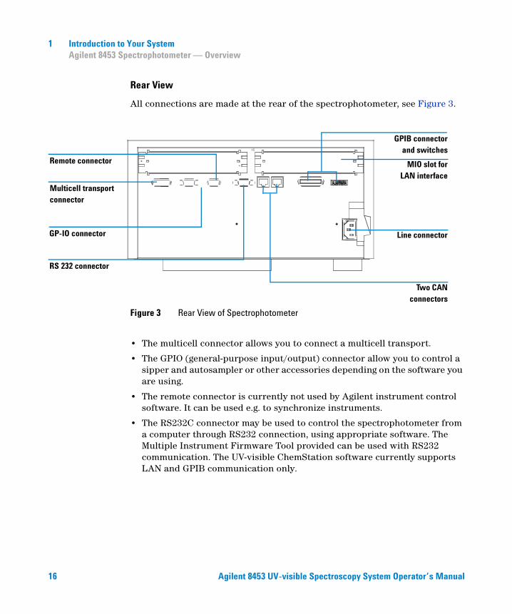
All connections are made at the rear of the spectrophotometer, see Figure 3.
• The multicell connector allows you to connect a multicell transport.
• The GPIO (general-purpose input/output) connector allow you to control a sipper and autosampler or other accessories depending on the software you are using.
• The remote connector is currently not used by Agilent instrument control software. It can be used e.g. to synchronize instruments.
• The RS232C connector may be used to control the spectrophotometer from a computer through RS232 connection, using appropriate software. The Multiple Instrument Firmware Tool provided can be used with RS232 communication. The UV-visible ChemStation software currently supports LAN and GPIB communication only.
Figure 3 Rear View of Spectrophotometer
Line connector
GPIB connectorand switches
Multicell transport connector
GP-IO connector
RS 232 connector
Remote connector
Two CANconnectors
MIO slot forLAN interface
16 Agilent 8453 UV-visible Spectroscopy System Operator’s Manual

Introduction to Your System 1Agilent 8453 Spectrophotometer — Overview
• The GPIB connector is used to connect the spectrophotometer with a computer. The 8-bit configuration switch module next to the GPIB connector determines the GPIB address of your spectrophotometer. The switches are preset to a default address recognized by the operating software from Agilent.
Only a single controller must be connected to the spectrophotometer at a time.
• The MIO board slot is reserved for a LAN interface board.
• The accessory board slot is reserved for future use.
• The power input socket does not have a voltage selector because the power supply has wide-ranging capability, for more information see your Service Manual Chapter 1 “Specifications”. There are no externally accessible fuses, because automatic electronic fuses are implemented in the power supply. The security lever at the power input socket prevents that the spectrophotometer cover is taken off when line power is still connected.
Side of the Spectrophotometer
On the right side of the spectrophotometer is a double door for access to the lamps. For exchanging lamps both doors, the plastic door and the sheet-metal door must be opened. Safety light switches are automatically turning off the lamps when the inner sheet metal door is opened.
Agilent 8453 UV-visible Spectroscopy System Operator’s Manual 17

1 Introduction to Your SystemGeneral Purpose Agilent ChemStation Software for UV-visible Spectroscopy — Overview
General Purpose Agilent ChemStation Software for UV-visible Spectroscopy — Overview
This section gives an overview of the elements of the user interface implemented with your Agilent ChemStation software and the data analysis concept behind. It explains how data are processed and what the advantages of this processing are on a practical point of view.
18 Agilent 8453 UV-visible Spectroscopy System Operator’s Manual
Introduction to Your System 1General Purpose Agilent ChemStation Software for UV-visible Spectroscopy — Overview
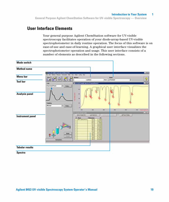
User Interface Elements
Your general purpose Agilent ChemStation software for UV-visible spectroscopy facilitates operation of your diode-array-based UV-visible spectrophotometer in daily routine operation. The focus of this software is on ease-of-use and ease-of-learning. A graphical user interface visualizes the spectrophotometer operation and usage. This user interface consists of a number of elements as described in the following sections.
Menu bar
Tool bar
Analysis panel
Instrument panel
Method name
Mode switch
Tabular results
Spectra
Agilent 8453 UV-visible Spectroscopy System Operator’s Manual 19

1 Introduction to Your SystemGeneral Purpose Agilent ChemStation Software for UV-visible Spectroscopy — Overview
Menu
The more traditional menu interface at the top of the Agilent ChemStation window allows to control all operations.When you choose an item from the menu bar a list of commands and submenus is displayed. An operation is performed by choosing a command (mouse click or ENTER key).
Toolbar
The tool bar below the menu bar shows buttons with symbols, icons, which allow direct access to basic operations such as printing result reports, loading methods, and saving methods and data.
Side Panels
The panels on the left side are the analysis panel and instrument panel. The size and position of these panels are fixed but are a function of your display’s resolution. The minimum resolution is 600 × 800 pixels.
Analysis Panel
The analysis panel gives you a graphical visualization of the current context in which you are working. In addition it provides access to the setup dialog of your actual task by means of the Setup button.
20 Agilent 8453 UV-visible Spectroscopy System Operator’s Manual

Introduction to Your System 1General Purpose Agilent ChemStation Software for UV-visible Spectroscopy — Overview
Instrument Panel
The instrument panel is below the analysis panel. It visualizes and controls your sampling devices and spectrophotometer. Part of the graphical elements on this panel are active items, for example, to switch lamps on or off, or run a peristaltic pump.
You can recognize the active areas by a pointer change when you move the mouse across the area. A mouse click in such an active position brings up a small menu with selections, or simply performs an operation.
In addition you can select a sampling system from the list of available systems. Its parameters can be adjusted by means of the Setup button.
Agilent 8453 UV-visible Spectroscopy System Operator’s Manual 21

1 Introduction to Your SystemGeneral Purpose Agilent ChemStation Software for UV-visible Spectroscopy — Overview
View
The area on the right side of the side panels offers you a view on a certain aspect of your current task. A view consists of one or more separate windows. These windows provide information in mainly a graphical or a tabular representation. You may see a graph showing your measured sample spectra and a table with the calculated results.
Views are usually handled automatically by the operation you performed, but you may also use the view menu’s commands to select the view you are interested in.
22 Agilent 8453 UV-visible Spectroscopy System Operator’s Manual

Introduction to Your System 1General Purpose Agilent ChemStation Software for UV-visible Spectroscopy — Overview
Software Structure
To reduce complexity of operation the software is divided into specific applications, called modes. In addition levels of operation are available and support for data evaluation sessions without spectrophotometer control.
Agilent ChemStation Sessions
Your Agilent ChemStation belongs to the Agilent’s ChemStation family of instrument control software. An installation of Agilent ChemStation software can control up to four different UV-vis instruments based on a single PC. Each of these instruments has its own session
If you start a session, its name is indicated in the main application’s window title bar, for example, Agilent 845x UV-visible System[1].
Each instrument session is available for data analysis only and for instrument control. An instrument control session has the appendix (Online) and can be started as the first instance only on your PC. In addition a data analysis sessions, which has the appendix (Offline), can be launched. The offline session allow recalculations based on stored data and is useful in the development process of an analytical method.
Agilent 8453 UV-visible Spectroscopy System Operator’s Manual 23

1 Introduction to Your SystemGeneral Purpose Agilent ChemStation Software for UV-visible Spectroscopy — Overview
Operation LevelsThe operation levels manager level and operator level apply to all modes and allow managing an application and running an application only. In the managing level of an application usually a method is developed and stored permanently to disk. The manager level of operation is password protected. This assures the integrity of predefined methods and operation sequences.
In the operator level only a reduced set of functions is available. Especially functions which may affect the integrity of an analytical procedure are not available. But on the other hand, an operator may use their own settings. This gets flagged on the tool bar and is be indicated on printed reports.
Agilent ChemStation Modes
The Agilent ChemStation modes are application oriented. Each mode has its own mode-specific menu, panels, operations and set of views. Your general purpose software for UV-visible spectroscopy is the platform for all modes. It is split into a Standard mode, an Execute Advanced Method mode and a Verification and Diagnostics mode.
According to your needs, modes are available for Advanced operation, Dissolution Testing runs, Multibath Dissolution Testing runs, Combined Reports evaluation, Kinetics measurements, Thermal Denaturation studies and Color Calculations.
These modes of operation can be switched within a running Agilent ChemStation session. All current raw data will be preserved during such a switch. This allows to look at your data with the focus on different aspects.
Most of the modes offer you the ability to define your analytical task by a set of parameters and, if necessary, data. A set of parameters and data can be saved to disk as a method. This allows you to repeat your analysis task under defined conditions simply by loading a method and running your samples.
24 Agilent 8453 UV-visible Spectroscopy System Operator’s Manual

Introduction to Your System 1General Purpose Agilent ChemStation Software for UV-visible Spectroscopy — Overview
Standard Mode Tasks
The Agilent ChemStation modes also offer the ability to focus on a certain aspect, many parameters have to be managed to customize a mode for a certain application. To overcome this complexity your standard mode offers an additional focus on tasks.
The standard mode of your general purpose software for UV-visible spectroscopy is oriented towards the most common tasks performed in a analytical laboratory that employs UV-visible spectroscopy. Four tasks are available:
• Fixed Wavelength
• Spectrum/Peaks
• Ratio/Equation
• Quantification
A task is selected and activated from the analysis panel’s selection box.
This task orientation lets you quickly adjust the software to give you the right view and answers based on your data. These tasks have been derived from a survey of the most common UV-visible spectroscopic tasks done on a routine basis in analytical laboratories. Historically these tasks have been developed on filter photometers or scanning spectrophotometers.
With your spectrophotometer you have the advantage that by default the entire UV-visible spectrum of your samples is available. So these four tasks do offer only different views to your data acquired.
A task switch within the Standard mode is much faster than an entire mode switch. An additional benefit of these tasks is that the definition of a method is done within a single dialog.
Agilent 8453 UV-visible Spectroscopy System Operator’s Manual 25

1 Introduction to Your SystemGeneral Purpose Agilent ChemStation Software for UV-visible Spectroscopy — Overview
Fixed Wavelength
The Fixed Wavelength task is used to look at measured sample data at up to six different wavelength. This data is available as absorbance, transmittance and first to fourth derivative.
Due to the spectral acquisition additional techniques such as internal reference or three-point, drop-line background corrections can be applied.
Spectrum/Peaks
In the Spectrum/Peaks task you are looking at absorbance minima and maxima. The focus here is more on the wavelength scale but you get the according absorbance readings in addition.
26 Agilent 8453 UV-visible Spectroscopy System Operator’s Manual

Introduction to Your System 1General Purpose Agilent ChemStation Software for UV-visible Spectroscopy — Overview
Ratio/Equation
The Ratio/Equation task is used to perform a user-definable equation based on measured data and sample information. An equation can be setup using sample data at up to six wavelengths, and weight and volume data entered with the samples measured. By means of an equation, for example, analysis results based on chemical test kits can be automatically calculated and reported. Another application is to use a ratio of data values to check for the identity or the purity of a sample.
Quantification
The Quantification task allows you to do single component analysis based on four different types of calibration curves and a set of standards. Due to the spectral acquisition in addition background corrections can be applied to your data.
The calibration can be optimized for your concentration range of interest by changing the wavelength used for calibration. A new calibration and a new analysis is automatically performed based upon your current standard data.
Agilent 8453 UV-visible Spectroscopy System Operator’s Manual 27

1 Introduction to Your SystemGeneral Purpose Agilent ChemStation Software for UV-visible Spectroscopy — Overview
Standard Mode Data Processing
General Data Processing
Although knowledge of the internal design of the data flow and processing in not required to use Agilent ChemStation software, it helps to understanding how Agilent ChemStation processes your data and how this processing is controlled by your method’s parameters.
The data processing can be easily described using a model of data containers and operations visualized in a flow diagram.
All basic data go into a raw data container. This container is empty when you start your Agilent ChemStation session and it will be filled by measuring data or loading data from a file.
The raw data container held the originally acquired data as specified with your acquisition parameters and stamped with, for example, acquisition date and time as well as the acquisition operator’s name.
Raw Data
ProcessedSpectra
UsedWavelength
Results
Spectral Processing
Data Access
Data Evaluation
28 Agilent 8453 UV-visible Spectroscopy System Operator’s Manual

Introduction to Your System 1General Purpose Agilent ChemStation Software for UV-visible Spectroscopy — Overview
SpectralProcessing
Your method defines how this data is analyzed. The first processing step is spectral processing. The processed raw data spectra are transferred automatically into a second container for processed spectra. This concept allows you to have a look at the results of this processing step by viewing the processed spectra container’s content. If you, for example, specified first derivative data type, the first derivative spectra of all your raw data are available in the processed spectra container after analysis. The type of spectral operation is defined by your method settings.
Used Wavelength
A next step in the data analysis process is the access to data for further evaluation specified in terms of wavelength and background correction operations such as an internal reference calculation or three-point, drop-line calculation.
This data is stored in the used wavelength container. In the Fixed Wavelength task, for example, a tabular view on these data is available with the Sample/Results Table window.
Results An additional step is the evaluation of the accessed data.
Agilent 8453 UV-visible Spectroscopy System Operator’s Manual 29

1 Introduction to Your SystemGeneral Purpose Agilent ChemStation Software for UV-visible Spectroscopy — Overview
In the Ratio/Equation task, for example, this used wavelength data is processed by an evaluation of the equation specified. This additional operation generates the calculation results. These calculated result values are filled into the results container.
The results are available with the Sample/Results Table.
Summary The generalized basic data processing is divided into three steps.
1 spectral processing
2 data access
3 data evaluation
These steps are always performed in the above order identically for all spectra in the raw data container. The results are placed in the results container. The previous content of the processed spectra, used wavelength and results container is replaced.
30 Agilent 8453 UV-visible Spectroscopy System Operator’s Manual

Introduction to Your System 1General Purpose Agilent ChemStation Software for UV-visible Spectroscopy — Overview
Processing with Standards
In the forth task, in addition to your sample data, standards are used. This requires an extension to the above concept to handle standards. Two independent sets of containers, one for standards and another for samples have been implemented. All processing containers are doubled as well. As with the sample processing only, all evaluation steps are done in parallel on both the samples and the standards.
The evaluation in quantification is now a calibration using standards. The coefficients are calculated based on the method’s settings and the current standards in the Agilent ChemStation memory. This means results now become a function of a measured set of standards and the standard concentrations specified.
Raw Data
ProcessedSpectra
UsedWavelength
Results
Spectral Processing
Data Access
Data Evaluation
Raw Data
ProcessedSpectra
UsedWavelength
CalibrationResults
Calibration
Samples Standards
Agilent 8453 UV-visible Spectroscopy System Operator’s Manual 31

1 Introduction to Your SystemGeneral Purpose Agilent ChemStation Software for UV-visible Spectroscopy — Overview
These coefficients are then used to calculate concentration results for the samples currently in memory. The same processing steps applied to sample and standard data lead to the most precise results.
Advantages
The concept of a diode-array-based spectrophotometer in combination with powerful data evaluation based on Agilent ChemStation offers many advantages over traditional spectrophotometer systems. Some of these advantages from a practical point of view are briefly descibed below.
• Virtually Unlimited Number Of Standards
Due to this data analysis concept you can measure your standards before or after your samples and, besides the minimum required number of standards, you can use as many standards you like to use with your calibration.
• Easy Optimization
The availability of all raw data—samples and standards—means you can easily optimize your method’s settings by choosing a different calibration wavelength and re calibrating your system. And, the elimination of outliers in your calibration is possible by simply removing this standard from you standard data set.
32 Agilent 8453 UV-visible Spectroscopy System Operator’s Manual

Introduction to Your System 1General Purpose Agilent ChemStation Software for UV-visible Spectroscopy — Overview
• Calibrated Method
When you save your method the standards currently in memory are always saved with the method. After loading a method, you can directly analyze your samples.
• Optimization for a Particular Sample
In addition you may optimize your wavelength settings for a sample outside the linear range of your actual calibration. Due to the excellent wavelength reproducibility of your spectrophotometer, you can switch to a wavelength with a lower extinction coefficient for precise analysis of such a sample.
• Summary
The availability of spectral raw data offers you many additional opportunities to optimize your calibration and analysis for best results. This optimization can be done quickly just by setting new method parameters. You get new answers almost instantaneously. The data analysis concept applied assures consistent and reliable results.
Agilent 8453 UV-visible Spectroscopy System Operator’s Manual 33

1 Introduction to Your SystemGeneral Purpose Agilent ChemStation Software for UV-visible Spectroscopy — Overview
34 Agilent 8453 UV-visible Spectroscopy System Operator’s Manual

Agilent 8453 UV-visible Spectroscopy SystemOperator’s Manual
2Installation and Start Up
Installation Summary for Your Agilent 8453 General Purpose UV-visible System 36
Starting a Measurement Session 38
This chapter does not replace the information available with the Installing Your UV-visible Spectroscopy System manual. It is meant as a reminder of the key steps of the installation and the system startup.
35Agilent Technologies

2 Installation and Start UpInstallation Summary for Your Agilent 8453 General Purpose UV-visible System
Installation Summary for Your Agilent 8453 General Purpose UV-visible System
General
A detailed description of your Agilent 8453 general purpose UV-visible system is given with the manual Installing Your UV-visible Spectroscopy System. The summary reminds you of the key points of installation.
Spectrophotometer
✔ Make sure that your spectrophotometer has the LAN interface card installed.
✔ Check that your spectrophotometer is either connected to your PC directly using a crossover LAN cable or to your LAN using a direct connection.
✔ Check that your spectrophotometer is connected to a power outlet.
✔ Before you switch on your spectrophotometer, make sure that the Agilent Bootp Service is installed on your PC or your network administrator has assigned an IP address to your spectrophotometer. For details see the chapter “LAN Communication, Installation, Connection and Configuration” in your Installing Your UV-visible Spectroscopy System manual.
CAUTION Do not connect the LAN adapter of your PC to the CAN interface of the Agilent 8453 spectrophotometer, otherwise the LAN adapter of the PC will be seriously damaged, because the operating voltage of the CAN interface (12 V) is higher than the operating voltage of the LAN adapter (5 V).
WARNING Always operate your instrument from a power outlet which has a ground connection. Always use the power cord designed for your region.
36 Agilent 8453 UV-visible Spectroscopy System Operator’s Manual
Installation and Start Up 2Installation Summary for Your Agilent 8453 General Purpose UV-visible System
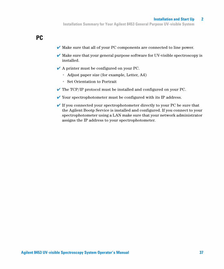
PC
✔ Make sure that all of your PC components are connected to line power.
✔ Make sure that your general purpose software for UV-visible spectroscopy is installed.
✔ A printer must be configured on your PC.
• Adjust paper size (for example, Letter, A4)
• Set Orientation to Portrait
✔ The TCP/IP protocol must be installed and configured on your PC.
✔ Your spectrophotometer must be configured with its IP address.
✔ If you connected your spectrophotometer directly to your PC be sure that the Agilent Bootp Service is installed and configured. If you connect to your spectrophotometer using a LAN make sure that your network administrator assigns the IP address to your spectrophotometer.
Agilent 8453 UV-visible Spectroscopy System Operator’s Manual 37

2 Installation and Start UpStarting a Measurement Session
Starting a Measurement Session
With a network connection to your spectrophotometer it is important that your spectrophotometer is recognized by the software. This requires the assignment of a unique IP address at power on time to your spectrophotometer. The assignment is either done by the Agilent BootP Service application running on your PC with a direct connection to the spectrophotometer or in a LAN by a server application on your LAN. Therefore it is important that either one of these applications is up and running before you switch your spectrophotometer on.
✔ Switch on your PC and boot your PC operating system. If a printer is connected to your system, switch the printer on.
✔ Make sure that the Agilent BootP Service is running or you are logged onto your LAN.
✔ Switch your spectrophotometer on and wait until the spectrophotometer’s indicator light turns to green. This process includes the spectrophotometer’s self test and takes about one minute. For details on the startup sequence see chapter “Installation and Start Up” in your Installing Your UV-visible Spectroscopy System manual.
✔ Launch your measurement session by pressing your operating system’s Start button and select Programs, UV-Visible ChemStations, Instrument 1 online.
✔ You are ready to use your system, if the blue busy status display on the system’s bottom message line turns off.
✔ The first measurement you have to perform is a reference measurement. After this alignment your are ready to measure absorbance data and spectra.
NOTE It takes about 15 minutes for the lamps to reach stable state conditions. For best results, do not perform measurements before this period of time has elapsed.
38 Agilent 8453 UV-visible Spectroscopy System Operator’s Manual

Agilent 8453 UV-visible Spectroscopy SystemOperator’s Manual
3Good Measurement Practices
General Considerations 40
Inserting a Cell 53
This chapter describes
• making measurements
• selecting material, optical specification and type of cell
• handling and maintaining cells
• checklist for good results
• solvents selection
• sample preparation
• use of filters
• stirring and temperature control of sample
• how to insert cells into the cell holder.
39Agilent Technologies

3 Good Measurement PracticesGeneral Considerations
General Considerations
There are many factors that can affect the results of your measurements. This section provides brief discussions of some of the more important ones.
Spectrophotometer Design
The sample compartment of the Agilent 8453 spectrophotometer is open. Unlike conventional instruments the Agilent 8453 does not suffer from ambient false light. The open sample area makes it easier to access it generally and to connect tubing to a flow cell or thermostattable cell holder.
Making Measurements
Blank (Reference) and Sample Measurement
Your spectrophotometer is a single beam instrument so you must measure a blank before you measure a sample. For the high accuracy measurements, the blank and the sample measurement should closely follow each other.
In general, a blank measurement should be repeated as often as is practical. Even in a thermally stable environment, a blank measurement should be taken at least every half hour to ensure accurate results.
Chemically, the only difference between the blank and the sample should be the presence of the analyte(s). For measurements with liquid samples, the blank should be a sample cell filled with the solvent you plan to use.
40 Agilent 8453 UV-visible Spectroscopy System Operator’s Manual

Good Measurement Practices 3General Considerations
Sample Cell Material
Quartz sample cells or sample cells with quartz face plates are required if you want to use the full 190 to 1100 nm wavelength range of your spectrophotometer.
If you plan on working only in the visible and/or short-wave near-infrared range of 350 to 1100 nm, you can use good quality glass cells.
Disposable plastic sample cells, for measurements in the range 400–1100 nm, are also available. The quality of these cells varies and they are generally not recommended.
Agilent 8453 UV-visible Spectroscopy System Operator’s Manual 41

3 Good Measurement PracticesGeneral Considerations
Optical Specifications of Cells
The accuracy of the readings of a diode-array spectrophotometer is very sensitive to spatial shifts of the measurement light beam. Cells having non parallel opposite faces, or so called wedge shaped cells, lead to a spatial shift of the light beam (see Figure 4). Therefore, the opposite cell walls illuminated by the analysis light beam have to very parallel. The parallelism is measured in terms of the angle between the two opposite cell walls. We recommend to use 10 mm path length cells with an angle which is below 0.1 degrees of an arc.
Figure 4 Shift of the Spectrophotometer Light Beam due to non Parallel Cell Walls
Light Beam in
Light Beam out
Light Beam in
ParallelCell Walls
Non-parallelCell Walls
Light Beam out
Light Beam In
Light Beam In
Light Beam Out
Light Beam Out
Non-parallelCell Walls
ParallelCell Walls
42 Agilent 8453 UV-visible Spectroscopy System Operator’s Manual

Good Measurement Practices 3General Considerations
Apertured Cells
In applications where sample volume is limited, apertured or microcells are used. The width of these cells is reduced to reduce the volume and the blank part of the cell must be blackened to avoid unwanted transmission and reflection through the side walls. If the side walls are not blackened the result will be poor photometric accuracy and, if different concentrations are measured, poor linearity.
The disadvantage of apertured and microcells is that part of the light beam is blocked. Not all the light passes through the sample and there can be some loss in sensitivity. See Figure 5 for recommended and Figure 6 for cells you should not use with the instrument.
Figure 5 Recommended Cells
Quartz cells Quartz cells with black apertures*
CAUTION * Quartz cells with black apertures smaller than 2 mm, when used with a multicell transport, can lead to measurements of poor reproducibility.
Agilent 8453 UV-visible Spectroscopy System Operator’s Manual 43

3 Good Measurement PracticesGeneral Considerations
Flow Cells
We recommend a sipper system with a flow cell for obtaining the high precision measurements. Using a flow cell eliminates the necessity of moving the cell between blank measurement and sample measurement. Also, the cell can be rinsed thoroughly with the solution to be measured.
The design of the flow cell should minimize entrapment of bubbles and flow channeling to provide the most reliable results.
Figure 6 Cells You Should Not Use With the Instrument
Quartz cells with transparent apertures, fluorescence cells, plastic cells
44 Agilent 8453 UV-visible Spectroscopy System Operator’s Manual

Good Measurement Practices 3General Considerations
Handling and Maintaining Cells
Passivating New Cells
When filling a non-passivated new cell with your sample, you will observe that air bubbles stick on the windows of your cell. To prevent the formation of sticky bubbles, rinse the cell with cleaning and passivating fluid (part number 5062-8529). The cleaning procedure you should apply is described on the label of the cleaning fluid container.
Cleaning Cells
The fats in fingerprints are significant absorbers in the UV region and, if left on optical surfaces, can cause erroneous results. Wipe off all fingerprints and contaminants before using a sample cell.
Use only high quality lens tissues (part number 9300-0761) and never dry the inside of a cell with lens tissues. Dry the inside of the cell with pressurized, oil free air, that prevents the cell from getting contaminated with tissue particles, or rinse the cell with blank or sample solution. Floating particles in the cell will deflect the light beam and so lead to a very poor quality of the measured spectrum.
Figure 7 Floating Particles in a Cell
Floating particles will deflect and scatter the light beam
Agilent 8453 UV-visible Spectroscopy System Operator’s Manual 45

3 Good Measurement PracticesGeneral Considerations
Lens tissues for glasses or other uses often contain detergents or lubricants which can affect your measurements. If possible avoid cleaning the faces of your cell between blank and sample measurements.
Handling Cells
Always install a cell so that it faces the same direction to minimize problems with cell non-uniformity. For best results with microcells, leave your sample cell clamped in position throughout the measurement sequence. Solutions should be removed and replaced by pipette or use flow cells.
Figure 8 Spectrum Taken With Floating Particles in the Light Path
CAUTION If glass pasteur pipettes are used, make sure that the optical windows of the cell are not touched or scratched by the pipette.
46 Agilent 8453 UV-visible Spectroscopy System Operator’s Manual

Good Measurement Practices 3General Considerations
Solvents
Your choice of solvents should be based primarily on the solvent’s absorbance characteristics over the wavelengths of interest, its suitability as a solvent for the analyte, and on experimental conditions. Table 1 lists common solvents and the lower limit of their useful wavelength range.
Table 1 Lower Limit of UV Transmission for Some Common Solvents
Lower Limit Solvent
180–195 nm Sulfuric acid (96%)WaterAcetonitrile
200–210 nm Cyclopentanen-HexaneGlycerol2,2,4-TrimethylpentaneMethanol
210–220 nm n-Butyl alcoholIsopropyl alcoholCyclohexaneEthyl ether
245–260 nm ChloroformEthyl acetateMethyl formate
265–275 nm Carbon tetrachlorideDimethyl sulfoxideDimethyl formamideAcetic acid
280–290 nm BenzeneToluenem-Xylene
Above 300 nm PyridineAcetoneCarbon disulfide
Agilent 8453 UV-visible Spectroscopy System Operator’s Manual 47

3 Good Measurement PracticesGeneral Considerations
When using volatile solvents such as acetone or methylene chloride, make sure that the sample cell is stoppered. Evaporation of a solvent does change the solute concentration and can cause solution noise due to solute convection currents. Both of these will affect the accuracy of your measurements. We also recommend stirring and temperature control when you use volatile solvents.
When using water as solvent we recommend using UV grade or HPLC grade water to reduce unwanted absorbance from impurities in the water. If you are using the sipper/sampler system the water should be degassed to avoid bubble formation in the flow cell, especially if the water comes from a pressurized water supply.
Sample Preparation
The sample cell should be rinsed three to five times with your intended solvent before you fill it with the pure solvent that will be used in the measurement. Turning the cell upside down on a small stack of absorbent tissues will help remove any residual solvent. This treatment will minimize contamination from previous experiments.
Samples which contain colloidal dispersions, dust or other particulate matter should be filtered, centrifuged or allowed to settle. If not, the overall attenuation-of-transmittance spectrum due to light scattering and/or reflection will hide the spectral information from the analyte.
WARNING Many of the solvents in Table 1 are hazardous. Be sure you fully understand their properties before using them.
48 Agilent 8453 UV-visible Spectroscopy System Operator’s Manual

Good Measurement Practices 3General Considerations
Photosensitive Samples
A few substances are very photosensitive. They degrade or undergo photochemical reactions if exposed to light. This can be easily seen by a decrease of sample absorbance over time.
Use of Filters
The shorter wavelength, higher-energy UV light is most likely to degrade photosensitive samples. If you have a problem, you can selectively block portions of the UV spectrum with a UV cut-off filter. An optical filter wheel assembly with three cut-off filters is available for the spectrophotometer. The cut-off wavelength of the filter you choose should be low enough that it does not eliminate important spectral information but high enough that it blocks the light that could degrade your sample. If you use a filter with your samples, you must use the same filter when you make your blank measurement.
Turning the D2-Lamp off
The short wavelength radiation leading to photodegradation comes from the light of the D2-lamp. For application where readings are taken at wavelengths above 400 nm, the D2-lamp can be turned off. The light intensity supplied by the Tungsten lamp is sufficient for a good signal to noise ratio over the wavelength range 400–1100 nm. When using cells with small apertures, you should check the signal to noise ratio by making sample measurements under conditions of your application.
Agilent 8453 UV-visible Spectroscopy System Operator’s Manual 49

3 Good Measurement PracticesGeneral Considerations
Stirring and Temperature Control
Solution homogeneity can be a problem, especially for viscous solutions. There are cases where, due to convection induced gradients, rapid absorbance changes may give irreproducible data. These changes can be observed spectroscopically by taking measurements with short integration times. To minimize convection effects keep the temperature of your sample the same as the cell holder or environmental temperature. Problems like these can also be minimized by using a thermostattable cell holder and/or a stirring module.
A similar effect can occur in cases of incomplete mixing. This is especially true where the specific gravities or miscibilities of the solvent and analyte are quite different. Again, stirring is a way to prevent this kind of problem.
In an unstirred cell, it is sometimes possible to observe local photodegradation of sensitive analytes. Because the actual volume of the sample in the light path is very small, stirring the sample will reduce the time any given analyte molecule is in the light path. This minimizes the photodegradation and increases homogeneity. Using a flow cell with continuous flow can yield similar results.
Checklist for Best Results
Cell:
✔ Cell is made of quartz or glass
✔ Apertured cells has black sides
✔ Apertured cells has an aperture greater than or equal to 3 mm
✔ Cell windows are free of fingerprints and other contamination
✔ Flow cell used instead of an apertured standard cell
Measurements:
✔ Solution in cell is free of floating particles
✔ Solution in cell and cell walls are free of bubbles
✔ Solution in cell is mixed homogeneously
✔ Blank measured on same solvent as sample
50 Agilent 8453 UV-visible Spectroscopy System Operator’s Manual
Good Measurement Practices 3General Considerations
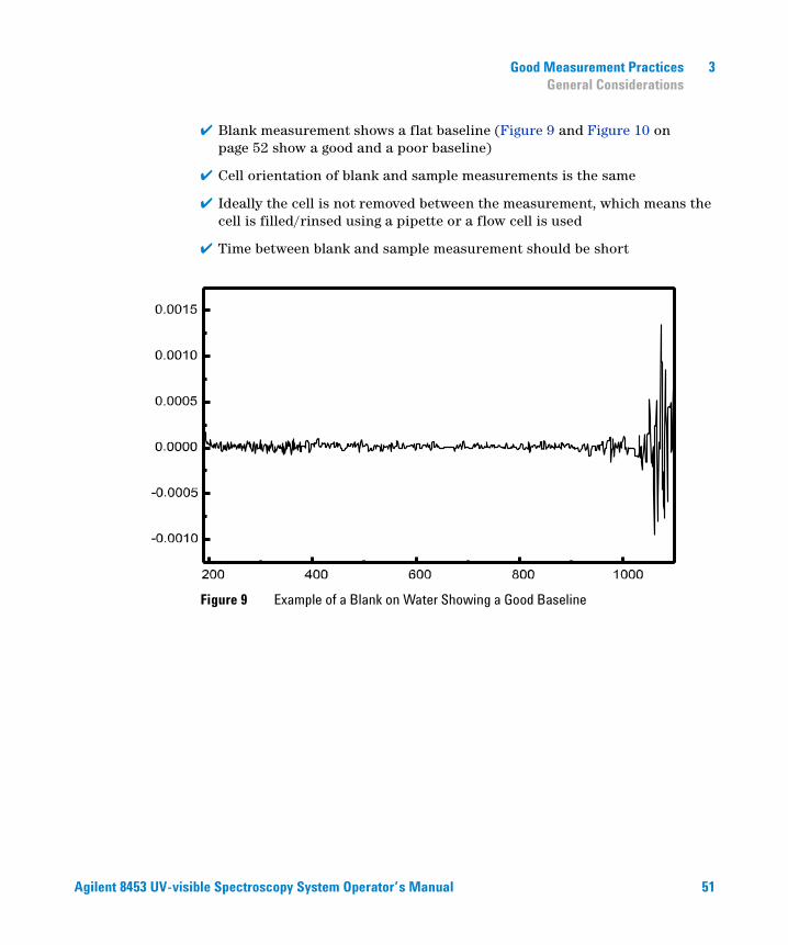
✔ Blank measurement shows a flat baseline (Figure 9 and Figure 10 on page 52 show a good and a poor baseline)
✔ Cell orientation of blank and sample measurements is the same
✔ Ideally the cell is not removed between the measurement, which means the cell is filled/rinsed using a pipette or a flow cell is used
✔ Time between blank and sample measurement should be short
Figure 9 Example of a Blank on Water Showing a Good Baseline
Agilent 8453 UV-visible Spectroscopy System Operator’s Manual 51

3 Good Measurement PracticesGeneral Considerations
Figure 10 Example of a Blank on Water with Bubbles Causing a Poor Baseline
NOTE If your blank or spectra shows artifacts similar to the one in Figure 10, see “Solvents" on page 47 to optimize the measurement procedure.
52 Agilent 8453 UV-visible Spectroscopy System Operator’s Manual

Good Measurement Practices 3Inserting a Cell
Inserting a Cell
Your spectrophotometer is shipped with the standard single-cell holder you first have to install in the sample compartment. This cell holder accommodates standard cells or flow cells. To insert a sample cell in the cell holder:
1 Move the locking lever to its up position. 2 Insert the sample cell, making sure you orient it correctly. The frosted (non-clear) sides of the sample cell should not be in the path of the light beam.
3 Lock the sample cell in place by pushing the locking lever back down.
Utmost care should be taken when using small volume flow cells and particularly any cells with less than a 2 mm aperture. Here is is imortant that the cells are properly centered in the light path. The cell holder is designed for cells with 15 mm center height. If applicable these cells should not be removed between the respective reference (blank) measurement and the sample measurement.
Agilent 8453 UV-visible Spectroscopy System Operator’s Manual 53

3 Good Measurement PracticesInserting a Cell
54 Agilent 8453 UV-visible Spectroscopy System Operator’s Manual

Agilent 8453 UV-visible Spectroscopy SystemOperator’s Manual
4Using your Agilent 8453 UV-visible Spectroscopy System
Starting Your First Measurement Session 56
Starting Your UV-visible Software 58
Measuring Caffeine Absorbance at 273 nm 59
Saving Your Parameters as a Method 62
Retrieving and Printing a Method 64
Saving and Retrieving Data 67
Print Preview of Reports 73
Finding the Caffeine Absorbance Maximum 76
Entering your Cell’s Path Length 80
Controlling your Sipper System 81
Using your Multicell Transport 83
Quantitative Analysis using a Calibration with Standards 86
How Can I Be Sure That My Agilent 8453 Works Properly? 93
How Can I Get a Deeper Understanding of UV-visible Spectroscopy? 96
When Do I Have to Measure a Blank? 98
55Agilent Technologies

4 Using your Agilent 8453 UV-visible Spectroscopy SystemStarting Your First Measurement Session
Starting Your First Measurement Session
1 Make sure that your Agilent 8453 UV-visible system has been installed correctly.
For details of installation see your Installing Your UV-visible Spectroscopy System manual.
2 Switch on your PC, monitor and printer.
3 Log on to your PC operating system.
Check your Agilent BootP Service is running using the Control Panel’s Administrative Tools Services dialog or make sure that your network administrator has integrated your Agilent 8453 spectrophotometer into your local network.
4 Switch on your Agilent 8453 spectrophotometer.
A running BootP service will now assign the configured IP address to your spectrophotometer. In the standard installation the Agilent BootP Service performs this task.
5 Start your measurement session by selecting Instrument 1 online from the menu.
Your Instrument Panel shows you the current state of the spectrophotometer and the Blank button is enabled.
56 Agilent 8453 UV-visible Spectroscopy System Operator’s Manual

Using your Agilent 8453 UV-visible Spectroscopy System 4Starting Your First Measurement Session
6 The first task you have to perform is to measure a reference. Typically the cell containing the solvent used with your samples is put in the measurement position and a blank measurement performed. To start this measurement, click the Blank button on your Instrument Panel or press the spectrophotometer’s Blank button.
A blank measurement is a reference measurement combined with the measurement of a baseline spectrum. A baseline spectrum gives you additional hints on the absorbance of the cell windows and the solvent. Areas with high noise indirectly indicate high absorbance.
7 The next measurement is your sample measurement. To get the most precise results, use the same cell in the same orientation to the measurement beam. Flush your cell about three times with your sample solution and start the measurement by clicking the Instrument Panel’s Sample button or by pressing the spectrophotometer’s Sample button.
NOTE For high precision measurements, wait until the spectrophotometer and the lamps have reached thermal equilibrium. The time required is a function of the environmental conditions. Your spectrophotometer should be ready after 45 minutes.
NOTE For details on how to mount your cell, see “Inserting a Cell" on page 53.
Agilent 8453 UV-visible Spectroscopy System Operator’s Manual 57

4 Using your Agilent 8453 UV-visible Spectroscopy SystemStarting Your UV-visible Software
Starting Your UV-visible Software
This section describes how you start an Agilent ChemStation session on your PC. If you want to perform measurements, you can start an online session, or you can start an offline session for optimizing the analytical parameters of a method, recalculating results or printing reports.
An online session can be started only as the first instance on your PC. In addition an offline session can be started in parallel. This allows you to optimize your method settings by direct comparison based on identical sets of data.
1 Switch on your PC, monitor and printer.
2 Log on to your PC’s operating system
3 Start your Agilent ChemStation session by selecting Instrument 1 online, for a measurement session, or Instrument 1 offline, for method optimization and data evaluation.
4 Enter your name to log on to your Agilent ChemStation session. If you protected your manager level by password, you must enter the correct password. The system will then come up with the last-used mode and method.
58 Agilent 8453 UV-visible Spectroscopy System Operator’s Manual

Using your Agilent 8453 UV-visible Spectroscopy System 4Measuring Caffeine Absorbance at 273 nm
Measuring Caffeine Absorbance at 273 nm
This section describes how you measure your caffeine sample that was shipped with your spectrophotometer. Measurement of this caffeine sample is also used for the IQ (installation qualification) of your Agilent 8453 spectrophotometer.
1 Make sure that you are in Standard mode. The mode is indicated on the toolbar of your Agilent ChemStation session.
2 Select the Fixed Wavelength task in the analysis panel’s selection box.
3 Click Setup in the analysis panel to open the parameter dialog.
Agilent 8453 UV-visible Spectroscopy System Operator’s Manual 59

4 Using your Agilent 8453 UV-visible Spectroscopy SystemMeasuring Caffeine Absorbance at 273 nm
4 Type the wavelength of interest in the Wavelengths section of the Fixed Wavelength(s) Parameters dialog. Adjust your spectral display to a wavelength range from 190 nm to 400 nm in the Display spectrum section. Click OK to set your parameters.
5 Fill your 1 cm path length quartz cell with distilled water. Lift the lever at the left side of your cell holder. Put the cell in the cell holder and make sure the transparent windows face towards the font and the back of the spectrophotometer. Push the lever down to secure your cell in the cell holder.
60 Agilent 8453 UV-visible Spectroscopy System Operator’s Manual
Using your Agilent 8453 UV-visible Spectroscopy System 4Measuring Caffeine Absorbance at 273 nm
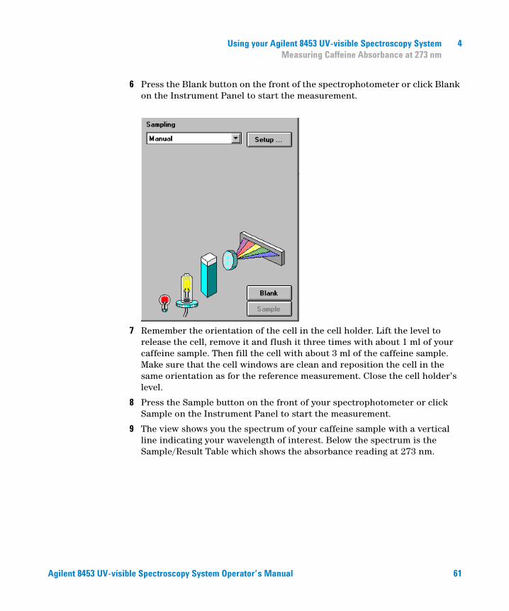
6 Press the Blank button on the front of the spectrophotometer or click Blank on the Instrument Panel to start the measurement.
7 Remember the orientation of the cell in the cell holder. Lift the level to release the cell, remove it and flush it three times with about 1 ml of your caffeine sample. Then fill the cell with about 3 ml of the caffeine sample. Make sure that the cell windows are clean and reposition the cell in the same orientation as for the reference measurement. Close the cell holder’s level.
8 Press the Sample button on the front of your spectrophotometer or click Sample on the Instrument Panel to start the measurement.
9 The view shows you the spectrum of your caffeine sample with a vertical line indicating your wavelength of interest. Below the spectrum is the Sample/Result Table which shows the absorbance reading at 273 nm.
Agilent 8453 UV-visible Spectroscopy System Operator’s Manual 61

4 Using your Agilent 8453 UV-visible Spectroscopy SystemSaving Your Parameters as a Method
Saving Your Parameters as a Method
This section describes how to save your settings for a future Agilent ChemStation session. Simply by loading your method you adjust your Agilent ChemStation to repeat your measurement. A library of methods facilitates routine laboratory work.
Let’s assume that your current settings are defining your method to analyze a caffeine sample. To be able to repeat such an analysis all set parameters can be stored permanently to disk. This allows you to load such a method on your system or even transfer such a method to your colleague with a Agilent ChemStation system.
1 Choose Save Method As… from the File menu or click the icon.
62 Agilent 8453 UV-visible Spectroscopy System Operator’s Manual

Using your Agilent 8453 UV-visible Spectroscopy System 4Saving Your Parameters as a Method
2 This displays the Save Method As… dialog box. Type the method name in the File name field, for example, Caffeine.m. Click OK to save your method.
NOTE If you generate many methods, you can use Options & Infos… from the Method menu to add text for documentation purposes and to simplify method access. This displays the Method Options & Information dialog box. In the Method Information section you can enter a sort descriptive text which becomes part of your method.
Agilent 8453 UV-visible Spectroscopy System Operator’s Manual 63
4 Using your Agilent 8453 UV-visible Spectroscopy SystemRetrieving and Printing a Method
Retrieving and Printing a Method
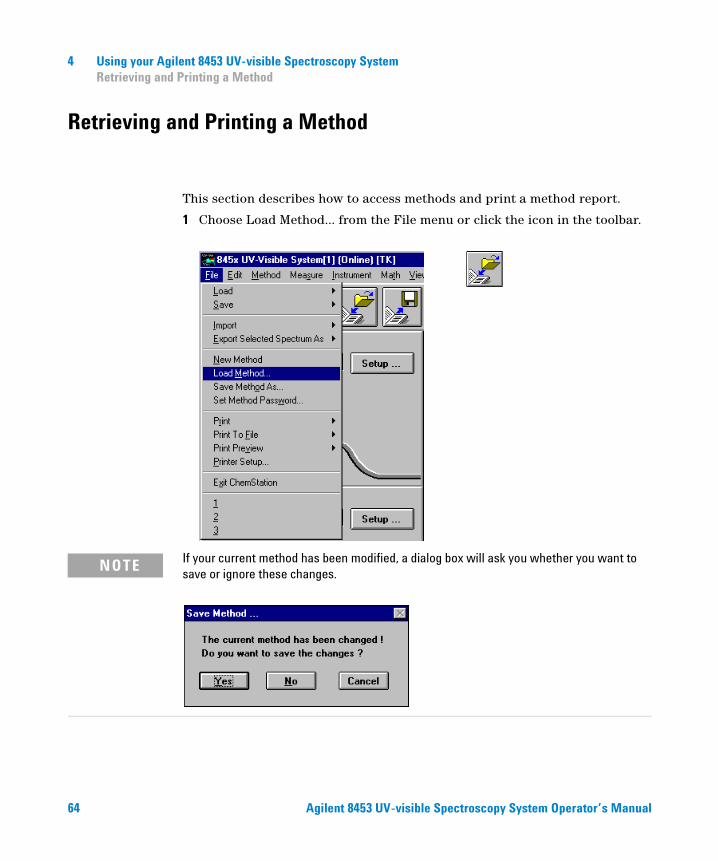
This section describes how to access methods and print a method report.
1 Choose Load Method… from the File menu or click the icon in the toolbar.
NOTE If your current method has been modified, a dialog box will ask you whether you want to save or ignore these changes.
64 Agilent 8453 UV-visible Spectroscopy System Operator’s Manual

Using your Agilent 8453 UV-visible Spectroscopy System 4Retrieving and Printing a Method
2 The Load Method… dialog is displayed. The selected method’s information is shown in the File Information section of the dialog box.
3 If you want to load this method, click OK.
NOTE Whenever you change a parameter of the current method, you get an indication in the toolbar’s modification field.
.
This triggers the reminder dialog mentioned above.
Agilent 8453 UV-visible Spectroscopy System Operator’s Manual 65

4 Using your Agilent 8453 UV-visible Spectroscopy SystemRetrieving and Printing a Method
4 To print a method, choose Print, Method from File menu.
NOTE To be able to print your method report, your printer must be properly configured and online. An alternative, if your printer is currently not online, is to view the print preview on the screen.
66 Agilent 8453 UV-visible Spectroscopy System Operator’s Manual

Using your Agilent 8453 UV-visible Spectroscopy System 4Saving and Retrieving Data
Saving and Retrieving Data
This section explains how you can save and retrieve measured data. This data can be used for archiving, for method development at a later stage, or for exchange with other Agilent ChemStations.
Your Agilent ChemStation has the ability to store and retrieve your data using a binary, checksum protected data format (extension *.sd,*.std). All current spectra -samples or standards- can be saved to disk for permanent storage. Save and load of data is possible using local and network drives. In addition a single spectrum can be selected for storage.
Saving your Samples
1 Choose Save, Samples As… from the File menu or click the toolbar icon.
Agilent 8453 UV-visible Spectroscopy System Operator’s Manual 67

4 Using your Agilent 8453 UV-visible Spectroscopy SystemSaving and Retrieving Data
2 You select one of your already existing data files in the File name selection box of the Save Spectra As… dialog or you type a valid file name into the File name edit box.
3 Click OK to start the operation.
NOTE A valid file name consist of eight alphanumeric characters and the file extension .sd or .std. Usually the extension .std is used for standards only.
If the file name exists already, a message box is displayed allowing you to abort or continue with the operation.
68 Agilent 8453 UV-visible Spectroscopy System Operator’s Manual

Using your Agilent 8453 UV-visible Spectroscopy System 4Saving and Retrieving Data
Saving a Selected Spectrum
1 Select the spectrum of interest in the graphic window.
Or, in the tabular Sample/Results Table window.
2 Choose Save, Selected Spectra As… from the File menu.
NOTE You may get the warning, Select/activate a window!, on the message line, if you did not select either the Overlaid Sample Spectra window or the Sample/Results Table window.
Agilent 8453 UV-visible Spectroscopy System Operator’s Manual 69

4 Using your Agilent 8453 UV-visible Spectroscopy SystemSaving and Retrieving Data
3 You select one of your already existing data files in the File name selector box of the Save Spectra As… dialog or you enter a valid file name into the File name edit box.
4 Press OK to start the operation.
70 Agilent 8453 UV-visible Spectroscopy System Operator’s Manual

Using your Agilent 8453 UV-visible Spectroscopy System 4Saving and Retrieving Data
Retrieving Spectra
1 Choose Load, Samples… from the File menu.
2 You select the data file in File name selector box of the Load Spectra to SAMPLES dialog box.
Agilent 8453 UV-visible Spectroscopy System Operator’s Manual 71

4 Using your Agilent 8453 UV-visible Spectroscopy SystemSaving and Retrieving Data
3 Click OK to start operation. The spectra available with your data file are added to the files currently in the Agilent ChemStation sample container.
Deleting Current Spectra
1 Choose Clear, Samples from the Edit menu or click the toolbar icon.
NOTE You can look at the File Information of your files by moving the selection in the file selector box. The content is always updated with the current selection.
NOTE Clear, Standards and Clear, Math. Results can be used to delete the current standards respectively the current mathematical results spectra from Agilent ChemStation memory.
72 Agilent 8453 UV-visible Spectroscopy System Operator’s Manual

Using your Agilent 8453 UV-visible Spectroscopy System 4Print Preview of Reports
Print Preview of Reports
Print preview allows you to look at the report in a separate Agilent ChemStation window based on the currently configured printer. All types of available reports can be checked page by page in the preview window. The number of pages generated and the layout also can be checked. In addition the currently displayed report can be printed.
Print Preview of a Results Report
The print previews work similarly for all available types of reports. The example below shows you how to preview your results report.
1 Choose Print Preview, Results from the File menu.
Agilent 8453 UV-visible Spectroscopy System Operator’s Manual 73

4 Using your Agilent 8453 UV-visible Spectroscopy SystemPrint Preview of Reports
2 The report generated will be displayed in the preview window.
NOTE Printing a results report requires you to have set all parameters properly and have data available for evaluation. If you do not have data, you may get the message No results present! on the message line.
74 Agilent 8453 UV-visible Spectroscopy System Operator’s Manual

Using your Agilent 8453 UV-visible Spectroscopy System 4Print Preview of Reports
This window allows you to look at your report page by page. Scroll bars are available if a page does not fit into the actual preview window.
In addition, you may use a different size for your preview display. Three sizes are available with the size selection box. Depending on your display resolution select the one which best fits your needs.
The following functions are available with the print preview window:
• The Prev and Next buttons allow you to browse through the report pages.
• A selection box allows to jump to a page directly.
• The Print button sends the report to the printer which is displayed in the lower left corner of the print preview window.
• The Close button closes your print preview window and discards the report shown.
Agilent 8453 UV-visible Spectroscopy System Operator’s Manual 75

4 Using your Agilent 8453 UV-visible Spectroscopy SystemFinding the Caffeine Absorbance Maximum
Finding the Caffeine Absorbance Maximum
This section describes how you find the absorbance maximum for your caffeine IQ sample.
1 Make sure that you are in the Standard mode. The mode is indicated on the tool bar of your Agilent ChemStation session.
2 Select the Spectrum/Peaks task in the analysis panel’s selection box.
3 Use the Setup button of the analysis panel to open the parameter dialog.
76 Agilent 8453 UV-visible Spectroscopy System Operator’s Manual

Using your Agilent 8453 UV-visible Spectroscopy System 4Finding the Caffeine Absorbance Maximum
4 Type 2 for the number of peaks to find and uncheck the valley find option. Set your data type to absorbance and adjust your spectral display to a wavelength range from 190 nm to 400 nm in the dialog’s Display spectrum section. Click OK to set your parameters.
5 Fill your 1-cm path-length quartz cell with distilled water. Lift the lever at the left side of your cell holder. Put the cell in the cell holder and make sure the transparent windows face towards the font and the back of the spectrophotometer. Push the lever down to secure your cell in the cell holder.
Agilent 8453 UV-visible Spectroscopy System Operator’s Manual 77
4 Using your Agilent 8453 UV-visible Spectroscopy SystemFinding the Caffeine Absorbance Maximum
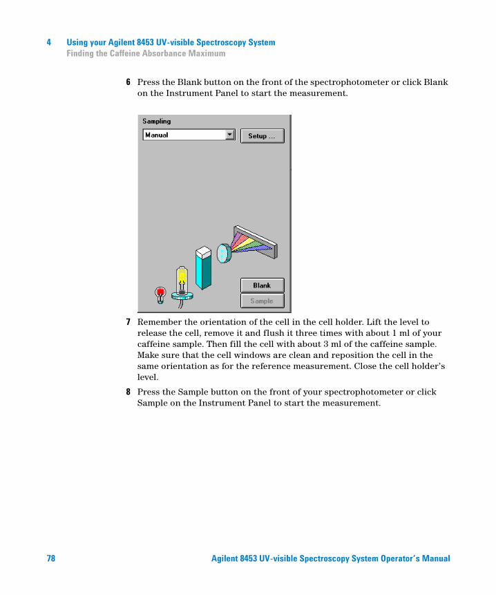
6 Press the Blank button on the front of the spectrophotometer or click Blank on the Instrument Panel to start the measurement.
7 Remember the orientation of the cell in the cell holder. Lift the level to release the cell, remove it and flush it three times with about 1 ml of your caffeine sample. Then fill the cell with about 3 ml of the caffeine sample. Make sure that the cell windows are clean and reposition the cell in the same orientation as for the reference measurement. Close the cell holder’s level.
8 Press the Sample button on the front of your spectrophotometer or click Sample on the Instrument Panel to start the measurement.
78 Agilent 8453 UV-visible Spectroscopy System Operator’s Manual

Using your Agilent 8453 UV-visible Spectroscopy System 4Finding the Caffeine Absorbance Maximum
9 The view shows you the spectrum of your caffeine sample. Two peaks were found marked and these annotated with the wavelength. Below the spectrum graph the Sample/Result Table shows the wavelength of the peaks found and the measured absorbance values.
Agilent 8453 UV-visible Spectroscopy System Operator’s Manual 79
4 Using your Agilent 8453 UV-visible Spectroscopy SystemEntering your Cell’s Path Length
Entering your Cell’s Path Length
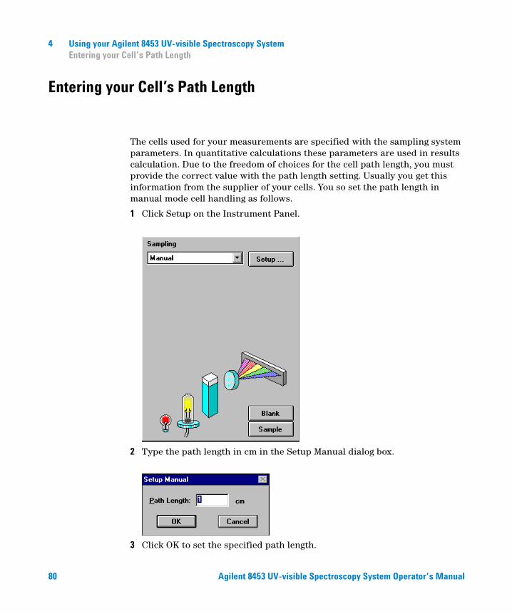
The cells used for your measurements are specified with the sampling system parameters. In quantitative calculations these parameters are used in results calculation. Due to the freedom of choices for the cell path length, you must provide the correct value with the path length setting. Usually you get this information from the supplier of your cells. You so set the path length in manual mode cell handling as follows.
1 Click Setup on the Instrument Panel.
2 Type the path length in cm in the Setup Manual dialog box.
3 Click OK to set the specified path length.
80 Agilent 8453 UV-visible Spectroscopy System Operator’s Manual

Using your Agilent 8453 UV-visible Spectroscopy System 4Controlling your Sipper System
Controlling your Sipper System
A sipper system transfers your sample by means of a peristaltic pump into a flow cell for the measurement. To control your sipper system through the Agilent ChemStation software, you have to adjust your current sampling system for sipper introduction.
In addition, due to the length of tubing, the dead volume of your flow cell and the flow rate of your pump, you adjust your sipper system parameters. For details see your Installing and Operating Your Sipper System manual.
1 Select the Sipper in the Instrument Panel selection box.
2 Click Setup on the Instrument Panel. Type the path length of your flow cell in cm and click OK.
3 Click Setup again and access the Sipper Parameter dialog by clicking Parameter. The parameters required can be determined using the Flow Test task of your Verification and Diagnostics mode.
Agilent 8453 UV-visible Spectroscopy System Operator’s Manual 81

4 Using your Agilent 8453 UV-visible Spectroscopy SystemControlling your Sipper System
4 Click OK in the Sipper Parameter dialog and click OK in the Sipper dialog to set the parameters.
NOTE Every measurement you start by clicking one of the Instrument Panel measurement buttons or by pressing the spectrophotometer buttons uses the sipper for sample introduction. Sipper introduction is also used by an automated sequence.
82 Agilent 8453 UV-visible Spectroscopy System Operator’s Manual

Using your Agilent 8453 UV-visible Spectroscopy System 4Using your Multicell Transport
Using your Multicell Transport
The multicell transport is a cell changer which allows you to position up to 8 cells in the measurement position automatically. You may use different cells in each measurement position. The path length can be specified individually for each of the cell positions.
1 Select Multicell (8-cell) in the Instrument Panel selection box.
2 Click Setup on the Instrument Panel. Type the path lengths of all cells used in cm and click OK.
NOTE For details about your multicell transport see your Installing and Operating Your Multicell Transport manual.
Agilent 8453 UV-visible Spectroscopy System Operator’s Manual 83

4 Using your Agilent 8453 UV-visible Spectroscopy SystemUsing your Multicell Transport
3 To move your cell for the next measurement into the measurement position, click the cell on the Instrument Panel or choose Multicell Transport Position from the Spectrophotometer menu to access Multicell transport Control dialog. In the Multicell Transport Control you press one of the position buttons to move the multicell transport.
84 Agilent 8453 UV-visible Spectroscopy System Operator’s Manual

Using your Agilent 8453 UV-visible Spectroscopy System 4Using your Multicell Transport
NOTE In an automated sequence the multicell transport can be used for automatic sample introduction. A maximum of 8 samples can be introduced. If you specify more than 8 measurements you get the warning:
You may also control an existing 7 position multicell transport. The major differences are that you have no separate reference position and one cell position less.
Agilent 8453 UV-visible Spectroscopy System Operator’s Manual 85
4 Using your Agilent 8453 UV-visible Spectroscopy SystemQuantitative Analysis using a Calibration with Standards
Quantitative Analysis using a Calibration with Standards
Your quantitative analysis task is based on a calibration with standards. After a successful calibration the measured standards can become part of your method. Such a method can be used directly for quantitative analysis of samples.
After having setup your method calibrated samples can be analyzed. Several views of both your standards and the calibration as well as on your samples and results are available.
As a quick introduction a calibration using Beer’s law with a single standard and the analysis of a sample are described. Further, the only limitation on the number of samples and standards is the memory capacity of your Agilent ChemStation.
For the practical experiment we use the IQ caffeine sample as standard and a 1:1 dilution with distilled water as sample. For the calibration we use absorbance data at 273 nm.
86 Agilent 8453 UV-visible Spectroscopy System Operator’s Manual

Using your Agilent 8453 UV-visible Spectroscopy System 4Quantitative Analysis using a Calibration with Standards
Setup
1 Make sure that you are in the Standard mode. The mode is indicated on the tool bar of your Agilent ChemStation session.
2 Select the ‘Quantification’ task in the analysis panel’s selection box.
3 A new task panel is displayed and the Quantification Parameters dialog is opened automatically.
NOTE If you are already in the Quantification task, use the Setup on the analysis panel to open the parameter dialog.
Agilent 8453 UV-visible Spectroscopy System Operator’s Manual 87

4 Using your Agilent 8453 UV-visible Spectroscopy SystemQuantitative Analysis using a Calibration with Standards
4 Setup your analysis wavelength at 273 nm (Use wavelength), type Caffeine for the Analyte name, set the Calibration curve type to Linear, select Concentration entry and use mg/l as Unit. Check the Prompt for standard information and the Prompt for sample information. Select Absorbance as Data type and set Display spectrum From 190 nm To 340 nm.
5 Click OK to set your parameters.
NOTE Now you are ready to run your measurements.
88 Agilent 8453 UV-visible Spectroscopy System Operator’s Manual

Using your Agilent 8453 UV-visible Spectroscopy System 4Quantitative Analysis using a Calibration with Standards
Calibration
1 Fill your 1-cm path-length quartz cell with distilled water. Lift the lever at the left side of your cell holder. Put the cell in the cell holder and make sure the transparent windows face towards the front and the back of the spectrophotometer. Push the lever down to secure your cell in the cell holder.
2 Press the Blank button on the front of the spectrophotometer or click Blank on the Instrument Panel to start the measurement.
3 Remember the orientation of the cell in the cell holder. Lift the level to release the cell, remove it and flush it three times with about 1 ml of your caffeine sample. Then fill the cell with about 3 ml of the caffeine sample. Make sure that the cell windows are clean and reposition the cell in the same orientation as for the reference measurement. Close the cell holder’s level.
4 Press the Standard button on the front of your spectrophotometer or click Standard on the Instrument Panel to start the measurement.
Agilent 8453 UV-visible Spectroscopy System Operator’s Manual 89

4 Using your Agilent 8453 UV-visible Spectroscopy SystemQuantitative Analysis using a Calibration with Standards
5 Enter your standard’s information in the Standard Information dialog box and click OK.
6 Your Agilent ChemStation software automatically calibrates and displays the calibration results. After a successful calibration the task panel’s calibration curve shows green. This indicates that your method is ready for analysis.
NOTE The Task panel’s Samples and Standards buttons can be used to switch your current view to the samples or standards view.
At this point you can also save your method for future use. See “Saving Your Parameters as a Method" on page 62 for more information.
90 Agilent 8453 UV-visible Spectroscopy System Operator’s Manual

Using your Agilent 8453 UV-visible Spectroscopy System 4Quantitative Analysis using a Calibration with Standards
Analysis
1 Remember the orientation of the cell in the cell holder. Lift the level to release the cell, remove it and flush it three times with about 1 ml of your caffeine sample (1:1 dilution with distilled water). Then fill the cell with about 3 ml of the caffeine sample. Make sure that the cell windows are clean and reposition the cell in the same orientation as for the standard measurement. Close the cell holder’s level.
2 Press the Sample button on the front of your spectrophotometer or click Sample on the Instrument Panel to start the measurement.
3 Enter your sample’s information in the Sample Information dialog box and click OK. The view switches to the samples and your quantitative results will be displayed with the Sample/Result table.
Agilent 8453 UV-visible Spectroscopy System Operator’s Manual 91

4 Using your Agilent 8453 UV-visible Spectroscopy SystemQuantitative Analysis using a Calibration with Standards
NOTE To save your data for future use or for documentation purposes, see “Saving and Retrieving Data" on page 67 for more information.
92 Agilent 8453 UV-visible Spectroscopy System Operator’s Manual

Using your Agilent 8453 UV-visible Spectroscopy System 4How Can I Be Sure That My Agilent 8453 Works Properly?
How Can I Be Sure That My Agilent 8453 Works Properly?
The quality of your measurement data is dependent on the performance of your spectrophotometer. For a full performance verification external standards are required. Standard kits are available for operational qualification and performance verification (OQ/PV). OQ/PV kits for the 8453 are available as part numbers 5063-6503 and 5063-6521.
A quick check without the need of standards can be performed by the Verification and Diagnostics mode’s self test. This test can be performed always after starting the spectrophotometer.
Agilent 8453 Self test
1 Make sure that you are in the Verification and Diagnostics mode. The mode is indicated on the tool bar of your Agilent ChemStation session.
2 Select the Self-Test task in the analysis panel’s selection box.
Agilent 8453 UV-visible Spectroscopy System Operator’s Manual 93
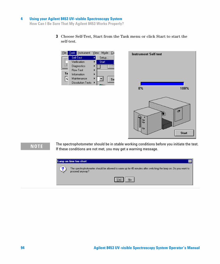
4 Using your Agilent 8453 UV-visible Spectroscopy SystemHow Can I Be Sure That My Agilent 8453 Works Properly?
3 Choose Self-Test, Start from the Task menu or click Start to start the self-test.
NOTE The spectrophotometer should be in stable working conditions before you initiate the test. If these conditions are not met, you may get a warning message.
94 Agilent 8453 UV-visible Spectroscopy System Operator’s Manual

Using your Agilent 8453 UV-visible Spectroscopy System 4How Can I Be Sure That My Agilent 8453 Works Properly?
4 The self-test results are displayed with pass/fail criteria.
NOTE Self-test results can be stored with the spectrophotometer. Storing the self-test results with the spectrophotometer allows you to monitor the performance over time. Graphical representations of the self-test histories can be generated.
Agilent 8453 UV-visible Spectroscopy System Operator’s Manual 95

4 Using your Agilent 8453 UV-visible Spectroscopy SystemHow Can I Get a Deeper Understanding of UV-visible Spectroscopy?
How Can I Get a Deeper Understanding of UV-visible Spectroscopy?
The basic principles of UV-visible spectroscopy are available with your help system. The information contained in the Tutorial’s Basics of UV-Visible Spectroscopy covers Basic Principles through to details of Derivative Spectroscopy.
In addition, solutions to selected topics in UV-visible analysis are described. There you can find help on topics such as Enhancing Sensitivity or Determining Purity.
96 Agilent 8453 UV-visible Spectroscopy System Operator’s Manual

Using your Agilent 8453 UV-visible Spectroscopy System 4How Can I Get a Deeper Understanding of UV-visible Spectroscopy?
More specific examples, including data, are available in the Examples section of the Standard Mode help. These can be used to run your Agilent ChemStation software for the special purpose described.
Agilent 8453 UV-visible Spectroscopy System Operator’s Manual 97
4 Using your Agilent 8453 UV-visible Spectroscopy SystemWhen Do I Have to Measure a Blank?
When Do I Have to Measure a Blank?
The measurement data acquired by your spectrophotometer is instrument independent. To achieve this independency, a reference measurement must be performed. All consecutive measurements are referring to the last measured reference.
In the Agilent ChemStation software, the reference measurement is combined with a baseline measurement. The baseline displayed is information about the quality of the current reference. In absorbance mode the data should be close to 0 AU and in transmission mode the data should be close to 100%.
Typically reference measurements for dissolved samples are made on the cell filled with the solvent used. Here, in addition, the absorbance properties of the cell and the solvent are influencing the reference data. In wavelength ranges where your solvent or cell is absorbing, the noise of the baseline spectrum is high. Reliable sample data cannot be expected in these areas.
Therefore new reference or blank measurements are required when
• you change your measurement cell or its orientation relative to the measurement position
• you use a different solvent or event a different lot of the same solvent
• the time between your reference measurement and the sample measurement get too long
• the time conditions are depending on the aging rate of your lamps and possible changes of your environmental conditions—typically the last blank measurement should not be older than half an hour.
98 Agilent 8453 UV-visible Spectroscopy System Operator’s Manual

Index
Aabsorbance 26
high 57absorbance maximum 76accessing lamps 17accessory slot 17accurate results 40acetic acid 47acetone 47acetonitrile 47acquisition
date 28time 28
active area 21active item 21active position 21Agilent 8453 36Agilent 8453 general purpose UV-visible
system 56Agilent Bootp Service 36, 38Agilent ChemStation
analysis panel 59, 76family 23graphical window 69log on 58measurement session 56method 62mode 24offline session 58online session 58password 58
preview sizes 75print preview 73printer display 75samples 72session 23session online 57workstation 32
ambient light 14analysis 91analysis panel 20, 93analysis setup
calibration 88concentration unit 88data type 88display 88prompt for sample information 88wavelength 88
analytes 40analytical task 24analyze 62apertured cells or cuvettes 43apertures 49application
specific 23
Bbackground correction 26, 27Beer’s law 86benzene 47blank 38, 40, 50blank push button 15bootp service 56bubble formation 48busy 38
Ccaffeine 59calculate 32calculation
results 80calibration 27, 31, 86, 89
coefficients 31curve 27
carbon disulfide 47carbon tetrachloride 47cell
path length 80, 81, 83cell changer 83chloroform 47cleaning cells 45collimated beam 10colloidal dispersions 48command 20common solvents 47compartment for sample 12concentration 32concentration range 27connection
network 9connector
GPIB 17GPIO 16multicell transport 16remote 16RS232 16
correctionfor stray light 10, 12
Agilent 8453 UV-visible Spectroscopy System Operator’s Manual 99

Index
current context 20current task 22cut-off filter 49cut-off wavelength 49cyclohexane 47cyclopentane 47
Ddata 28
absorbance 86access 29, 30archieve 67clear 72clear math. results 72clear standards 72evaluation 30file extension 68file information 72file name 68file selector box 72format 67load 67local storage 67network transfer 67removing 72replace 68retrieve 67, 71save 67save samples as 67saving selected data 69storage 67
degassed 48derivative 26derivative spectroscopy 96description
of instrument 14determining purity 96deuterium lamp 10
development of an analytical method 23dialog
fixed wavelength(s) parameters 60method options & information 63
dimethyl formamide 47dimethyl sulfoxide 47diode array 13, 32door to access lamps 17dust 48
Eenhancing sensitivity 96entrapment of bubbles 44equation 25, 30ethyl acetate 47ethyl ether 47examples 97extinction coefficient 33
Ffalse light 14, 40filter for stray-light correction 10, 12fixed wavelength 25, 26, 59flow cell 44flow cells 53flow test 81front view of spectrophotometer 14
Gglass cells 41glycerol 47GPIB
connector 17GPIO connector 16grating 10, 13
Hhandling cells 46highest precision measurements 44holographic grating 10, 13homogeneity 50HPLC grade water 48
Iidentity 27indicator 15installation 36installation qualification 59instrument
construction 10description 14electronic assemblies 10layout 10mechanical assemblies 10warm up 57
instrument panel 21instrument session 23internal reference 26, 29IP address 36, 37, 38, 56isopropyl alcohol 47
Llamps 11
access through door 17deuterium 10tungsten 10
LANcrossover cable 36
LAN interfaceJet Direct 36Talk2Lab 36
lens 10
100 Agilent 8453 UV-visible Spectroscopy System Operator’s Manual

Index
lens tissues 45levels of operation 23light beam 42, 45line power 37
input socket 17switch 14
liquid samples 40logged 38
Mmain application window 23making measurements 40manager level 24, 58maximum 25measure
standard 89standard information 90
measure push buttons 15measurement
blank 57noise 57reference 57sample 57, 91sample information 91
menu 20message line 38methanol 47method 24, 28, 31, 32, 62
calibrated 33, 86current 65information 65last used 58load 64load method 64modified 64name 63options & information 63parameter 28parameters 62
print preview 66printing 64, 66report 64retrieve 64save method as 62store 62
methyl formate 47minimum 25MIO board
slot 17mode 23
advanced 24color calculations 24combined reports 24dissolution testing 24execute advanced method 24kinetics 24last used 58multibath dissolution testing 24standard 24, 59, 76, 87switch 24thermal denaturation 24verification and diagnostics 24, 93
mouse cursor 21multicell transport 83
7-cell 858-cell 83connector 16
m-xylene 47
Nn-butyl alcohol 47network
administrator 36, 37connection 38local 56
n-hexane 47nominal spectral slit width 12
Ooffline 23online 23open sample area 40operating system 38operation 20operation levels 24operator level 24operator name 28optical filter 49optical specifications of cells 42optical surfaces 45optical system 10optimization 32outliers 32
Ppaper
orientation 37size 37
parallelism 42parameter dialog 76particulate matter 48passivating new cells 45path length
setup 80PC 38peak find 77performance verification 93photochemical reactions 49photodegradation 49photodiode array 13photosensitive substances 49pipette 46plasma discharge 11plastic
door 17
Agilent 8453 UV-visible Spectroscopy System Operator’s Manual 101

Index
plastic sample cells 41pointer symbol 21poor linearity 43poor photometric accuracy 43printer 37, 38
configured 73processed spectra 29processing 28
spectral 29standards 31
pumpperistaltic 81
purity 27push buttons 15
blank 15sample 15standard 15stop 15
pyridine 47
Qquantification 25, 87quantitative analysis
of samples 86ready for analysis 90
quartz sample cells 41
Rradiation source 10rapid absorbance changes 50ratio 25raw data 28rear view of spectrophotometer 16recalculation 23recommended cells 43reference 38remote connector 16
reportresults 73
result 32results 29
precise 57routine work 62RS232C
connector 16
Ssample 40, 51
compartment 12push button 15
sample cell 40, 48sample data 31sample information 27sample/result table 61, 69, 79sampling device 21sampling interval 12sampling system 80
manual 80sipper 81
security lever 17self test 93
histories 95results 95start 94working conditions 94
sensitivity 43session
data analysis only 23instrument control 23
set of parameters 24settings 62setup dialog 20sheet-metal
door 17shine-through aperture 11shutter 10, 11side panel 20signal to noise ratio 49single beam instrument 40
sipper 81flow test 81parameter 81
sipper system 44sipper/sampler system 48slit 10, 13slit width 12slots for MIO and accessory boards 17software
general purpose 9, 18solute convection 48solution 50solution noise 48solutions 96
determining purity 96enhancing sensitivity 96
solvent 40, 57solvent suitability 47solvents 47source lens 10, 11source of radiation 10spectral acquisition 27spectral operation 29spectral processing 30spectral raw data 33spectrograph 12
lens 10slit 10
spectrophotometer 32, 36front view 14rear view 16
spectroscopy system 9spectrum 25standard 27, 31
external 93standard cells 53standard push button 15standard single-cell cell holder 53standards 86
current 31minimum required number 32number of 32
102 Agilent 8453 UV-visible Spectroscopy System Operator’s Manual

Index
status 38status indicator 15stirring 48stirring module 50stop push button 15stoppered sample cell 48stray-light correction 10, 12sulfuric acid 47symbol 20
Ttask
fixed wavelength 25, 26, 59orientation 25quantification 25, 27, 86quantitative analysis 86ratio/equation 25, 27, 30spectrum/peaks 25, 26
TCP/IP protocol 37temperature control 48test kit 27thermostattable cell holder 50three point drop line 26, 29toluene 47tool bar 20transmittance 26trimethylpentane
2,2,4-trimethylpentane 47tungsten lamp 10tutorial
basic principles 96basics of UV-visible spectroscopy 96derivative spectroscopy 96
Uunderstanding
Agilent ChemStation processing 28used wavelength 29useful wavelength range of solvents 47user definable equation 27user interface
elements 19UV grade water 48UV-visible spectroscopy
basics 96
Vvalley find 77view 22, 25
calibration 86results 86, 91samples 61, 79standards 86
viscous solutions 50volatile solvents 48volume 27
Wwarning
no results present! 74water 47wavelength 29wavelength reproducibility 33wedge shaped cells 42weight 27width of slit 12window 22
graphical 22sample/results table 29tabular 22
Agilent 8453 UV-visible Spectroscopy System Operator’s Manual 103

Index
104 Agilent 8453 UV-visible Spectroscopy System Operator’s Manual


© Agilent Technologies 2002, 2003-2007
Printed in Germany 04/07
*G1115-90030**G1115-90030*G1115-90030
www.agilent.com
Agilent Technologies
In This Book
To be able to use your new Agilent 8453 UV-visible spectroscopy system quickly, this book gives you step-wise procedures and examples for basic operations and tasks.

sa
Agilent 8453 UV-visible Spectroscopy System
Service Manual

Agilent Technologies Deutschland GmbHHewlett-Packard-Strasse 876337 WaldbronnGermany
Copyright Agilent Technologies 2000
All rights reserved. Reproduction, adaption, or translation without prior written permission is prohibited, except as allowed under the copyright laws.
Part No. G1103-90004
Edition 02/00
Printed in Germany
Warranty
The information contained in this document is subject to change without notice.
Agilent Technologies
makes no warranty of
any kind with regard to
this material,
including, but not
limited to, the implied
warranties or
merchantability and
fitness for a particular
purpose.
Agilent Technologies shall not be liable for errors contained herein or for incidental or consequential damages in connection with the furnishing, performance, or use of this material.
WARNING
For details of safety, see Safety Information on page 154.
Warning Symbols Used
In This Book
The apparatus is marked with this symbol when the user should refer to the instruction manual in order to protect the apparatus against damage.
Eye damage may result from directly viewing the light produced by the deuterium lamp used in this product. Always turn off the deuterium lamp before opening the metal lamp door on the side of the instrument.
!

Service Manual
Agilent 8453 UV-visible Spectroscopy System

In This Book
This handbook is intended for the technical reader who needs background
information about the Agilent 8453 spectrophotometer and potential repairs.The handbook contains specifications of the spectrophotometer as well as descriptions of front and back panels, for example, where to connect accessories. Electronics are explained at block-diagram level. There is a detailed section about troubleshooting to help find a defective subassembly, such as an electronic board, in case the spectrophotometer does not operate any more. Part replacement procedures as well as an exploded view with part numbers are given for ordering and replacing assemblies.
For information about installation of the system including the spectrophotometer, computer and accessories, see the Installing Your
UV-Visible Spectroscopy System handbook.
Use Chapter 1 “Specifications” to check the specifications of the spectrophotometer.
Use Chapter 2 “Theory of Operation” if you want an overview of the optics, front and rear panel functions or if you need explainations about the electronics or pin assignment of cables.
Use Chapter 3 “Diagnostics and Troubleshooting” to find explainations of status and error messages and a logical approach to troubleshooting.
Use Chapter 4 “Maintenance and Repair” for exchanging parts, such as lamps and electronical or mechanical items and cleaning lenses,
Use Chapter 5 “Parts and Materials” to locate parts and find out their part numbers.
Use Chapter 6 “Interfacing” to set the 8-bit switch for RS232 comunication and to reset the spectrophotometer in case of problems when loading a new firmware. Use the Installing Your UV-Visible Spectroscopy System handbook for information about GPIB settings.
4

Contents
1 Specifications
Specifications of the Agilent 8453 UV-visible
spectrophotometer 9
Physical Specifications 11Performance Specifications 12Source of Standards 14
2 Theory of Operation
An overview of the instrument, the theory of operation and con-
trol, as well as external communication and internal
connections 15
Instrument Overview 18
Optical System Overview 19Instrument Description 22Instrument Layout and Construction 26
Theory of Operation and Control 28
Electronics Overview 29The Main Power Supply Assembly 32Spectrophotometer Processor Main (SPM) Board 34Spectrophotometer Data Acquisition (SDA) Board 37Spectrophotometer Lamp Supply (SLS) Board 39Spectrophotometer Interface (SSI) Board 42Firmware Description 43
External Communication 50
External Cables 51
5

Contents
External Connectors 56
Internal Connections 62
Connector Definitions 63
3 Diagnostics and Troubleshooting
Explainations of status and error messages and a logical ap-
proach to troubleshooting 67
Front Panel Status and Power Switch LEDs 69Error Messages 71General Troubleshooting Hints 80
4 Maintenance and Repair
Procedures for exchanging parts, such as lamps and electronic
or mechanical items, and for cleaning lenses 93
Maintenance 94
Cleaning the Instrument 95Exchanging the Deuterium or Tungsten Lamp 96Cleaning the Stray Light Filter 101Cleaning the Lenses 103
Repair Procedures 108
Removing and Replacing Covers 109Exchanging Keyboard and Key Pad 116Exchanging or Upgrading Internal Memory 118
6

Contents
Exchanging the SPM Board 120Exchanging the Optical Unit 122Exchanging the Shutter Assembly 124Exchanging the Fan Assembly 126Exchanging SDA Board 128Exchanging SLS Board 130Exchanging the Main Power Supply 133
5 Parts and Materials
Exploded views of repairable parts and part number listings
for ordering replacement and exchange parts 137
Exploded Views and Part List 138
6 Interfacing
Communicating and interfacing through GPIB and
RS-232C 145
Setting the 8-Bit Configuration Switch 146
7

Contents
8

1
1 Specifications
Specifications of the Agilent 8453 UV-visible spectrophotometer

Specifications
The Agilent 8453 spectrophotometer is a single-beam, microprocessor-controlled, UV-visible spectrophotometer with collimating optics. With its diode-array technology, the spectrophotometer is much faster than comparable conventional instruments—with more precision, more sensitivity and more reproducible results. Accessories include special cell holders, peristaltic pumps, autosampler, a multicell transport, a Peltier temperature control accessory, and valve unit and valve-pump controller.
The spectrophotometer can be either controlled from HP and non-HP personal computers equipped with Agilent ChemStation software for UV-visible spectroscopy (personal computers used should be certified by UL1950), or from the dedicated handheld controller that comes with the Agilent 8453E UV-vis spectroscopy system.
10

SpecificationsPhysical Specifications
Physical Specifications
WARNING If you use the spectrophotometer at environmental temperatures
higher than 50 °C (122 °F) the backplane may get hot.
Table 1 Physical Specifications
Type Specification Comments
Dimensions 34.4 cm (13.5 inches) wide56.0 cm (22.0 inches) deep18.5 cm (7.3 inches) high
Weight 16.5 kg (36.3 lbs)
Line voltage 90–264 V AC Wide-ranging capability
Line frequency 47–63 Hz
Power consumption 220 VA Maximum
Ambient operating temperature 0–55 °C (32–131 °F) See WARNING on page 11
Ambient non-operating temperature -40–70 °C (-4–158 °F)
Humidity <95%, at 25–40 °C (77–104 °F) Non-condensing
Operating altitude Up to 2000 m (6,500 ft)
Non-operating altitude Up to 4600 m (14,950 ft) For storing the instrument
Safety standards: IEC, CSA, UL Installation Category II, Polution Degree 2
11

SpecificationsPerformance Specifications
Performance Specifications
Performance specifications are measured after a minimum 1 hour from cold start or from lamp turn-on, with no cell or filter unless specified, see Table 2. Cold start in this context means that the spectrophotometer had been stored for some hours at room temperature.
Table 2 Performance Specifications
Type Specification Comments
Wavelength range 190–1100 nm
Slit width 1 nm
Resolution > 1.6 Toluene in hexane, ratio of absorbances at 269 and 266 nm
Stray light < 1.0 % At 200 nm, solution of 1.2% KCl, blank scan on air, 5 s integration time; (EP* method)**
< 0.05 % At 220 nm, solution of 10 g/l NaI, blank scan on air, 5 s integration time; (ASTM method)
< 0.03 % At 340 nm, solution of 50 g/l NaNO2, blank scan on air, 5 s integration time; (ASTM method)
Wavelength accuracy < ± 0.5 nm NIST 2034 standard, using transmittance peak minima; wavelength in NIST certificate are interpolated for 1.5 nm bandwidth from the values given for 2 nm and 1 nm bandwidth; uncertainty of standard from NIST certificate (typically ±0.1 nm) is added to the specification; 99-point spline function is used; 0.5 s integration time
Wavelength reproducibility < ± 0.02 nm Ten consecutive scans with NIST 2034 standard; 0.5 s integration time
Photometric accuracy < ± 0.005 AU NIST 930e standard at 1 AU, at 440.0, 465.0, 546.1, 590.0, and 635.0 nm, the expanded uncertainty from NIST certificate is added to the specification; 0.5 s integration time
Photometric accuracy < ± 0.01 AU Potassium dichromate in 0.01 N H2SO4 at 235, 257, 313, 350 nm; blank scan on 0.01 N H2SO4; 0.5 s integration time (EP method)
12
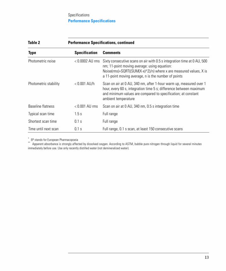
SpecificationsPerformance Specifications
Photometric noise < 0.0002 AU rms Sixty consecutive scans on air with 0.5 s integration time at 0 AU, 500 nm; 11-point moving average: using equation: Noise(rms)=SQRT((SUM(X-x)^2)/n) where x are measured values, X is a 11-point moving average, n is the number of points
Photometric stability < 0.001 AU/h Scan on air at 0 AU, 340 nm, after 1-hour warm up, measured over 1 hour, every 60 s, integration time 5 s; difference between maximum and minimum values are compared to specification; at constant ambient temperature
Baseline flatness < 0.001 AU rms Scan on air at 0 AU, 340 nm, 0.5 s integration time
Typical scan time 1.5 s Full range
Shortest scan time 0.1 s Full range
Time until next scan 0.1 s Full range, 0.1 s scan, at least 150 consecutive scans
* EP stands for European Pharmacopoeia** Apparent absorbance is strongly affected by dissolved oxygen. According to ASTM, bubble pure nitrogen through liquid for several minutesimmediately before use. Use only recently distilled water (not demineralized water).
Table 2 Performance Specifications, continued
Type Specification Comments
13

SpecificationsSource of Standards
Source of Standards
Wavelength Accuracy
The NIST 2034 Holmium Oxide solution is available from:
U.S. Department of CommerceNational Institute of Standards and TechnologyStandard Reference Materials ProgramBldg. 202, Room 204GaithersburgMD 20899USATel. (301) 975 6776
Photometric Accuracy
The NIST 930e standard is available from NIST, see above address.
Other Standards
All other standards can be prepared using the appropriate material recommended in the EP or ASTM procedures.
Agilent Technologies Standards Kit
All liquid standards required by the EP or ASTM are available in snap-open ampules from Agilent Technologies. These standards are easy to handle, inexpensive and traceable. The OQ/PV chemical standards kit I (order number 5063-6503) contains potassium dichromate, sodium nitrite, sodium iodide and toluene in hexane. The OQ/PV chemical standards kit II (order number 5063-6521) contains holmium oxide in perchloric acid.
14

2
2 Theory of Operation
An overview of the instrument, the theory of operation and control, as well as external communication and internal connections

Theory of Operation
This chapter has four sections:
• “Instrument Overview” on page 18,
• “Theory of Operation and Control” on page 28,
• “External Communication” on page 50, and
• “Internal Connections” on page 62.
16

Theory of Operation
17

Instrument Overview
This section gives an overview of the optical system and explains the
instrument front and back panel. It also explains the layout and construction of the instrument including the electronic and mechanical assemblies inside the instrument.18

Theory of OperationOptical System Overview
Optical System Overview
Optical System
The optical system of the spectrophotometer is shown in Figure 1. Its radiation source is a combination of a deuterium-discharge lamp for the ultraviolet (UV) wavelength range and a tungsten lamp for the visible (VIS) and short wave near-infrared (SWNIR) wavelength range. The image of the filament of the tungsten lamp is focused on the discharge aperture of the deuterium lamp by means of a special rear-access lamp design which allows both light sources to be optically combined and share a common axis to the source lens. The source lens forms a single, collimated beam of light. The beam passes through the shutter/stray-light correction filter area then through the sample to the spectrograph lens and slit. In the spectrograph light is dispersed onto the diode array by a holographic grating. This allows simultaneous access to all wavelength information. The result is a fundamental increase in the rate at which spectra can be acquired.
Figure 1 Optical System of Spectrophotometer
Lamps
The light source for the UV wavelength range is a deuterium lamp with a shine-through aperture. As a result of plasma discharge in a low pressure deuterium gas, the lamp emits light over the 190 nm to approximately 800 nm wavelength range. The light source for the VIS and SWNIR wavelength range is a low-noise tungsten lamp. This lamp emits light over the 370 nm to 1100 nm wavelength range.
Tungsten lamp
Source lens
Deuterium lamp
Shutter/stray light filter
Cuvette
Photodiode array
Source lens
Slit
Grating
19

Theory of OperationOptical System Overview
Source Lens
The source lens receives the light from both lamps and collimates it. The collimated beam passes through the sample (if one is present) in the sample compartment.
Shutter
The shutter is electromechanically actuated. It opens and allows light to pass through the sample for measurements. Between sample measurements it closes to limit exposure of sample to light. If the measurement rate is very fast, you can command the shutter to remain open (ChemStation software) or it stays open automatically (handheld controller software).
Stray-Light Correction Filter
In a standard measurement sequence, reference or sample intensity spectra are measured without and then with the stray-light filter in the light beam. Without the filter the intensity spectrum over the whole wavelength range from 190–1100 nm is measured. The stray-light filter is a blocking filter with 50 % blocking at 420 nm. With this filter in place any light measured below 400 nm is stray light. This stray-light intensity is then subtracted from the first spectrum to give a stray-light corrected spectrum. Depending on the software, you can switch off the stray light correction (ChemStation software) in case you want to do very fast repetitive scans or it is switched off automatically (handheld controller software).
Sample Compartment
The spectrophotometer has an open sample compartment for easier access to sample cells. Because of the optical design a cover for the sample area is not required. The spectrophotometer is supplied with a single-cell cell holder already installed in the sample compartment. This can be replaced with the Peltier temperature control accessory, the thermostattable cell holder, the adjustable cell holder, the long path cell holder or the multicell transport. All of these optional cell holders mount in the sample compartment using the same quick, simple mounting system. An optical filter wheel is also available for use with the spectrophotometer and most of the accessories.
Spectrograph
The spectrograph housing material is ceramic to reduce thermal effects to a minimum. It main components of the spectrograph are the lens, the slit, the grating and the photodiode array with front-end electronics. The mean
20

Theory of OperationOptical System Overview
sampling interval of the diode array is 0.9 nm over the wavelength range 190 nm to 1100 nm. The nominal spectral slitwidth is 1 nm.
Spectrograph Lens
The spectrograph lens is the first of the parts which are collectively known as the spectrograph. It is mounted on the housing of the spectrograph. The spectrograph lens refocuses the collimated light beam after it has passed through the sample.
Slit
The slit is a narrow aperture in a plate located at the focus of the spectrograph lens. It is exactly the size of one of the photodiodes in the photodiode array. By limiting the size of the incoming light beam, the slit makes sure that each band of wavelengths is projected onto only the appropriate photodiode.
Grating
The combination of dispersion and spectral imaging is accomplished by using a concave holographic grating. The grating disperses the light onto the diode array at an angle proportional to the wavelength.
Diode Array
The photodiode array is the heart of the spectrograph. It is a series of 1024 individual photodiodes and control circuits etched onto a semiconductor chip. With a wavelength range from 190 nm to 1100 nm the sampling interval is nominal 0.9 nm.
21

Theory of OperationInstrument Description
Instrument Description
Your spectrophotometer is very easy to use. It has a line power indicator, a status indicator and some push buttons. All electrical connections are made at the rear of the instrument.
Front View
The front view of the spectrophotometer is shown in Figure 2. Notice that the sample compartment is open. Unlike conventional instruments the Agilent 8453 does not suffer from ambient stray light. The open sample area makes it easier to access for cuvette handling and to connect tubing to a flow cell or thermostattable cell holder. The spectrophotometer is shipped with the standard single-cell cell holder. Standard and accessory cell holders can be removed and replaced in seconds with few or no tools.
Figure 2 Front View of Spectrophotometer
The line power switch is located at the lower-left part of the instrument. Pressing it in turns on the instrument. It stays pressed in and shows a green light when the instrument is turned on. When the line power switch stands out and the green light is off, the instrument is turned off.
On the front panel of the spectrophotometer is a status indicator which will display different colors depending of the actual condition of the instrument.
Indicator
PushbuttonsLine power switch with green light
22

Theory of OperationInstrument Description
• Green—the instrument is ready to measure.
• Green, blinking—the instrument is measuring.
• Yellow—the instrument is in not-ready state, for example, turning one of the lamps on or if both lamps are switched off.
• Red—error condition, that is, the spectrophotometer does not pass one of the self-tests which are run when the spectrophotometer is turned on or an error occurred during operation. In this case the UV-Visible operating software gives a detailed error message and possible explanations are in the online help system and in Chapter 3 “Diagnostics and Troubleshooting”.
• Red, blinking—error condition of the spectrophotometer processor system. Because in this case there is no communication with the computer there will be no error message. The online help system and Chapter 3 “Diagnostics and Troubleshooting” give more information about troubleshooting.
NOTE When using an Agilent 8453E UV-vis spectroscopy system, you will only have access to the online help of the handheld controller, when there is no power loss at the CAN interface of the Agilent 8453 spectrophotometer.
The four measure push buttons on the front panel cause the following actions to be performed and the resulting data being sent to the computer.
• BLANK—the instrument takes a blank measurement. This comprises a reference measurement that is used in all subsequent sample measurements until a new blank measurement is taken. Following the reference measurement the baseline spectrum is measured and displayed on the PC.
• SAMPLE—the instrument takes a sample measurement or starts a series of measurements. This depends on the parameters set in your software.
• STANDARD—the instrument takes a measurement of a standard. Additional information such as concentration and so on, have to be entered in the operating software.
• STOP—the instrument and/or software aborts any ongoing activity and returns to a to ready state. The stop button is not supported when the handheld controller of the Agilent 8453E UV-vis spectroscopy system is used to control the spectrophotometer.
23
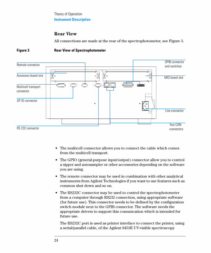
Theory of OperationInstrument Description
Rear View
All connections are made at the rear of the spectrophotometer, see Figure 3.
Figure 3 Rear View of Spectrophotometer
• The multicell connector allows you to connect the cable which comes from the multicell transport.
• The GPIO (general-purpose input/output) connector allow you to control a sipper and autosampler or other accessories depending on the software you are using.
• The remote connector may be used in combination with other analytical instruments from Agilent Technologies if you want to use features such as common shut down and so on.
• The RS232C connector may be used to control the spectrophotometer from a computer through RS232 connection, using appropriate software (for future use). This connector needs to be defined by the configuration switch module next to the GPIB connector. The software needs the appropriate drivers to support this comunication which is intended for future use.
The RS232C port is used as printer interface to connect the printer, using a serial/parallel cable, of the Agilent 8453E UV-visible spectroscopy
Line connector
GPIB connector and switches
Multicell transport connector
GP-IO connector
RS 232 connector
Remote connector
Two CAN connectors
MIO board slotAccessory board slot
24

Theory of OperationInstrument Description
system.
• The right CAN bus is used to connect the handheld controller of the Agilent 8453E UV-visible spectroscopy system to the spectrophotometer.
• The GPIB connector is used to connect the spectrophotometer with a computer. The 8-bit configuration switch module next to the GPIB connector determines the GPIB address of your spectrophotometer. The switches are preset to a default address recognized by the operating software from Agilent Technologies.
The GPIB port is not used when the handheld controller of the Agilent 8453E UV-visible spectroscopy system is connected to the spectrophotometer. However, the 8-bit configuration switch of the port must be set for GPIB communication.
• The MIO board slot is reserved for a LAN interface board.
• The accessory board slot is reserved for future use.
• The power input socket does not have a voltage selector because the power supply has wide-ranging capability, for more information see Chapter 1 “Specifications”. There are no externally accessible fuses, because automatic electronic fuses are implementeded in the power supply. The security lever at the power input socket prevents that the spectrophotometer cover is taken off when line power is still connected.
Side of the Instrument
On the right side of the instrument there is a door for exchanging the lamps. Behind this plastic door there is another sheet-metal door. Two independant safety light switches are implemented. They automatically turn off the lamps when the sheet metal door is opened.
25

Theory of OperationInstrument Layout and Construction
Instrument Layout and Construction
The industrial design of the spectrophotometer incorporates several innovative features. It uses the E-Pak concept for the packaging of electronics and mechanical assemblies. This concept is based upon the use of layers foam plastic spacers in which the electronic boards of the spectrophotometer are placed. This pack is then housed in a metal internal cabinet which is enclosed by a plastic external cabinet. The advantages of this packaging technology are:
• the plastic layers have air channels molded in them so that cooling air can be guided exactly to the required locations,
• the plastic layers help cushion the electronical and mechanical parts from physical shock, and
• the metal inner cabinet shields the internal electronics from electromagnetic interference and also helps to reduce or eliminate radio frequency emissions from the instrument itself.
26

Theory of OperationInstrument Layout and Construction
27

Theory of Operation and Control
This section explains the function of the electronics of the
spectrophotometer on block-diagram level. Each board and/or functional group is described in a separate module.28

Theory of OperationElectronics Overview
Electronics Overview
Figure 4 Electronics Block Diagram
The spectrophotometer includes a spectrograph which utilizes a processor-controlled photodiode array. Several processing steps and hardware boards are required to form spectra from the intensity counts derived from the diode array. Full spectra can be acquired, processed and transmitted every 0.1 s continuously, the only bottleneck being the PC speed. The instrument has its own onboard real-time clock and this allows the instrument to perform a series of time-based accessory control actions and
SPMspectrophotometer processor
main board
SLSspectrophoto-meterlamp supply board
SDAspectrophoto-meterdata acquisitionboard
SSIspectrophotometersipper interface
switches LED
spectrograph
SCI spectrograph connector interface
PDAphotodiode array
interfaces
MPSspectrophotome-ter main power
shutter
fan
deuteriumlamp
tungstenlamp
line power
29

Theory of OperationElectronics Overview
measurements without control from the PC and buffer the data until the PC wants to take it.
SPM—Spectrophotometer Processor Main Board
The spectrophotometer processor main (SPM) board receives DC power from the main power supply (MPS) and distributes it to a number of other modules. These include the spectrophotometer lamp supply (SLS) board, spectrophotometer data acquisition (SDA) board and from there the spectrophotometer sipper interface (SSI) board and the spectrograph with the diode array.
The SPM board interfaces to the controller, that is, the computer and other devices, such as pumps, valves, the multicell transport, RS232 and other peripheral devices. Shutter control allows for dark current or sample measurements and utilizes the stray light filter. Stray-light correction is calculated by combining information of two spectra, a spectrum measured with the stray-light correction filter and a spectrum without the stray-light correction filter in the light path. Memory for approximately 100 full spectra is available and two SIMM sockets for extending the memory (to be able to store several hundred spectra) are available.
SLS—Spectrophotometer Lamp Supply Board
The SLS board provides control and regulation for both, the tungsten and deuterium lamps.
Spectrograph
The spectrograph contains the PDA (photodiode array) which gives an analog signal proportional to the light level which falls on the individual photodiode during a defined period of time. The photodiode array is connected to the spectrophotometer data acqisition (SDA) board through the spectrograph connector interface (SCI) board. A temperature sensor is located on the diode-array for temperature compensation, that is, to reduce drift. This is especially important for the SWNIR part of the spectrum where drift with temperature is significant due to variation in the quantum efficiency of the photodiodes.
30

Theory of OperationElectronics Overview
SDA—Spectrophotometer Data Acquisition Board
On the SDA board, the signals from the photodiode array are adjusted to an appropriate level and converted to digital values by a 16-bit A/D converter. In addition, the SDA board controls the timing of the photodiode array. The firmware automatically converts data points which are taken at a 0.9-nm sampling interval from the diode array to deliver values at 1-nm interval to the controller.
SSI—Spectrophotometer Sipper Interface Board
This board collects the signals from the push buttons and controls the three-color LED located on the front panel of the spectrophotometer.
31
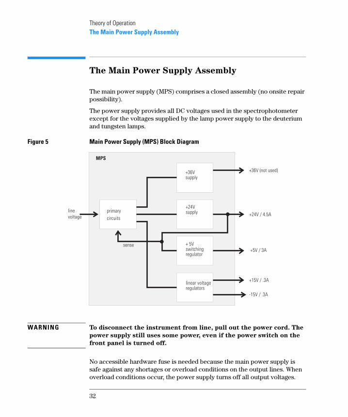
Theory of OperationThe Main Power Supply Assembly
The Main Power Supply Assembly
The main power supply (MPS) comprises a closed assembly (no onsite repair possibility).
The power supply provides all DC voltages used in the spectrophotometer except for the voltages supplied by the lamp power supply to the deuterium and tungsten lamps.
Figure 5 Main Power Supply (MPS) Block Diagram
WARNING To disconnect the instrument from line, pull out the power cord. The
power supply still uses some power, even if the power switch on the
front panel is turned off.
No accessible hardware fuse is needed because the main power supply is safe against any shortages or overload conditions on the output lines. When overload conditions occur, the power supply turns off all output voltages.
� � � �� � � � �
� � �� � � � �
� � �� � � � � � � � � �� � � � � � � � �
� � � � � � � � � � � � � � �� � � � � � � � � �
� � � � � � � � � � � � � � �
� � � � � � � � �
� � � � � � �
� � � � � � � �
! � � � � � � �
� � � �
� � � � � � �� � � " � �
� � � � � � � �
� � �
� � � � �
32

Theory of OperationThe Main Power Supply Assembly
Turning the line power off and on again resets the power supply to normal operation if the cause of the overload condition has been removed.
An overtemperature sensor in the main power supply is used to turn off output voltages if the temperature exceeds the acceptable limit (for example, if the cooling fan of the instrument fails). To reset the main power supply to normal operating conditions, turn the instrument off, wait until it is approximately at ambient temperature and turn the instrument on again.
Table 3 gives the specifications of the main power supply.
Table 3 Main Power Supply Specifications
Function Specification Comment
Line input 100–120 or 220–240 V AC ±10% Wide-ranging
Line frequency 50 or 60 Hz ±5%
Output 1 +24 V / 4.5 A
Output 2 +36 V Not used
Output 3 +5 V / 3 A
Output 4 +15 V / 0.3 A
Output 5 -15 V / 0.3 A
33

Theory of OperationSpectrophotometer Processor Main (SPM) Board
Spectrophotometer Processor Main (SPM)
Board
Figure 6 SPM Board
4 control
LEDs
8-bit
switch
HPIB
driver
CAN
driver
GPIO
driver
RS232
driver
multicell transport driver
APG remot-e
ASIC
application
specific
integrated
circuit
main
microprocessor
SSP
spectra and
signal processor
SIMM
memory
module
ASIC RAM
real time
clock
battery
PWM
driver
LEDs and switches
serial bus
SSP bus
control lines
sense
serial bus
SPM
memory
MPSmainpowersupply
SD
A b
oa
rd
shutter
fan
SL
S b
oa
rdS
DA
bo
ard
34

Theory of OperationSpectrophotometer Processor Main (SPM) Board
Main Microprocessor
The main microprocessor exchanges data with the ASIC through the core bus as well as with the memory, consisting of the battery backed-up, non-volatile random access memory (NVRAM), the system memory and the program memory. The program memory includes the firmware which can be updated by a download procedure from the computer. The battery for the NVRAM and the real-time clock is designed to last for more than 25 years under normal operating conditions.
Control lines provide communication to the SLS board, which in turn controls the deuterium and tungsten lamps. The main microprocessor comunicates to the SSP (spectra and signal processor) through a parallel bus.
ASIC—Application-Specific Integrated Circuit
The 304-pin application specific integrated circuit (ASIC) provides interfacing to external devices through drivers, including GPIB, CAN, APG Remote, and GPIO. It is also connected to the four control LEDs located near the connectors on the SPM board and the 8-bit configuration switch which is used to configure the address for the GPIB communication, baud rate for RS232 transfer, and so on. For switch settings, refer to the Installing Your
UV-Visible Spectroscopy System handbook.
In addition it controls the shutter and cooling fan through the PWM (pulse width modulation) driver. Operation of the cooling fan is sensed by the microprocessor.
SSP—Spectra and Signal Processor
The spectra and signal processor (SSP) uses a dedicated ASIC and RAM of 3 × 128 KB and converts the 1024 raw data values from the SDA board to intensity and absorbance values. Conversion and subsequent calculation to achieve absorbance values include the following tasks, listed in the sequence of processing:
1 dark current correction,
2 offset correction,
3 PDA temperature compensation,
4 stray-light correction,
5 absorbance calculation,
6 signal averaging (over integration time), and
35

Theory of OperationSpectrophotometer Processor Main (SPM) Board
7 variance calculation.
Communication between the spectra and signal processor (SSP) and the PDA front end processor (PFP) on the SDA board is established by a serial communication link. Processed data and synchronization signals for the PFP clock frequency are exchanged through the serial bus.
SIMM Memory Module
The SIMM memory module controlled by the dedicated ASIC is used to expand the memory to 2 MB (add 1 MB module, part number 1818-4271) or 2 × 4 MB (part number 1818-5784) to accomodate more spectra.
Firmware
For an outline of the firmware, see “Firmware Description” on page 43.
36

Theory of OperationSpectrophotometer Data Acquisition (SDA) Board
Spectrophotometer Data Acquisition
(SDA) Board
Figure 7 SDA Board
# $ #
# % � � & � � � �
� � � � � � � � � � � � �
� � ' � � � � ( ) * +
� � % � � � � � � � � � �
# % �
� � � � � � � � � � � � � � � � � � �
� � � � � � � � � � �
� � � � � � � �
& � � � � �
,-.�'����
,#/
�'����
,,.��'����
0 # 1 %
2 � /
� � � � � � � � � � � � �
# % � � � � � � � �
# % � � � � " � � � � � � � � � � � � � � �
� � � � � ' � � � � � � � � � � � � � � �
� � � � � � � ' � �
, % �
37

Theory of OperationSpectrophotometer Data Acquisition (SDA) Board
SCI—Spectrograph Connector Interface Board
The PDA, which includes control electronics for readout of the individual photodiodes, is mounted on the SCI (spectrograph connector interface) board. Gain switching is used to optimize the signal level to the dynamic range of the A/D converter on the SDA board. In addition, wavelength calibration data from the manufacturing process are stored in the resident EEPROM to provide both wavelength precision and accuracy.
PDA Signal Conditioning Electronics
Data is transferred from the photodiode array (PDA) through the spectrograph connector interface (SCI) board to the PDA signal conditioning electronics. The PDA signal conditioning electronics adjusts the signal levels to provide an appropriate output signal.
A/D Converter
The output signal from the PDA signal conditioning electronics is directed to the 16 bit /160 kHz A/D converter. Multiplexing is used to monitor the signal from the PDA temperature sensor which is used for temperature compensation.
PFP–PDA Front-End Processor
The PDA front end processor (PFP) utilizing an on board RAM and the EPLD (electronically programmable logic device) forwards the data from the 16 bit A/D converter to the SPM board. It provides timing and control for the photodiode readout and the A/D conversion.
Low-Pass Filter
Signals between the SPM board and the switches and LED on the spectrophotometer sipper interface (SSI) board are routed through a low-pass filter for RFI (radiated frequency interference) improvement.
38
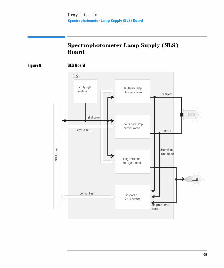
Theory of OperationSpectrophotometer Lamp Supply (SLS) Board
Spectrophotometer Lamp Supply (SLS)
Board
Figure 8 SLS Board
� � � � � � � � � � � � " �
& � � � " � � � � � � � � � � �
� � � � � � � � " � � � " �
� � � � � � � � � � � � � � �
� � � � � � � � � � � " �
� � � � � � � � � � � � � � �
� � � � � � � � � �
� � % � � � � � � � � � �
� � & � � � � � � � �
� � � � � � � �
,#/
�'����
� � � � � � � � ' � �
� � � � � � � � "
� � " � � � � � � �
� � � � � � � � � � � " �
� � � � �
� � � � �
& � � � " � � �
� � � � � � � � �
� � � � � � � � ' � �
, 1 ,
39

Theory of OperationSpectrophotometer Lamp Supply (SLS) Board
Deuterium Lamp Filament Control
During the ignition cycle two different voltage levels are applied to the filament of the deuterium lamp by the deuterium lamp filament control circuit. This control circuit is enabled by the processor on the SPM board.
Deuterium Lamp Current Control
The deuterium lamp current control circuit comprises two parts. One generates an ignition pulse of 600 V DC for the lamp, resulting in lamp ignition. After the ignition process this voltage is disabled. The second is a constant current source of 320 mA at an operating voltage between 50 and 105 V DC for stable operating conditions and light emission of the deuterium lamp. The deuterium lamp current control circuit is supervised by the processor on the SPM board.
Igniting the Deuterium Lamp
The deuterium lamp is heated with a voltage of 1.7 V DC for 1 s and afterwards a voltage 2.5 V DC for 9 s with currents between 2–10 A prior to ignition. The deuterium lamp current control circuit provides an ignition pulse to the lamp, resulting in lamp ignition. The filament control circuit disables the filament voltage if the lamp has been successfully ignited.
If the deuterium lamp has failed to ignite, the whole sequence is repeated. If after the second attempt the deuterium lamp did not ignite, an error message occurs.
Tungsten Lamp Voltage Control
Voltage to the tungsten lamp is generated by the tungsten lamp voltage control circuit which is enabled by the processor, resident on the SPM board. This circuit provides a constant voltage of 6 V DC with currents between 0.7– 0.9 A to light the tungsten lamp.
Diagnostic A/D Converter
The diagnostic A/D converter senses currents and voltages of the deuterium and tungsten lamps and converts the analog signals into digital values. The digital values are transferred via the control bus to the SPM board. When values are outside of the normal range, an appropriate error message is generated.
40

Theory of OperationSpectrophotometer Lamp Supply (SLS) Board
Safety Light Switches
When the sheet metal lamp door is removed and the instrument is still on, the safety light switches are activated and result in turn off of the deuterium and tungsten lamps.
The safety light switches provide shutdown in two different ways. One is a direct line to the deuterium lamp filament and current control circuits as well as the tungsten lamp voltage control circuit. The second is through the processor on the SPM board. The different ways are used to provide maximum reliability and safety.
41
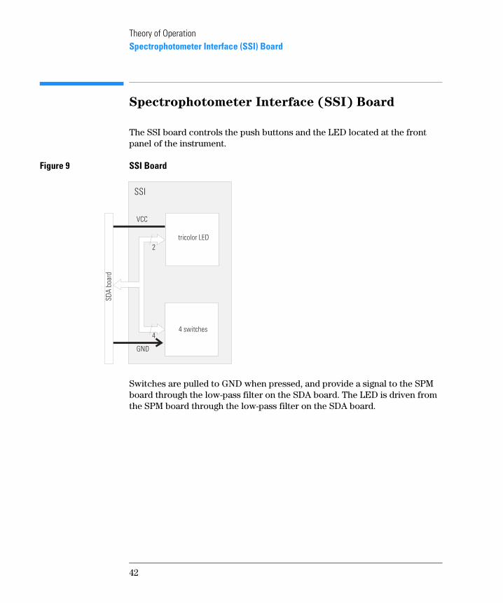
Theory of OperationSpectrophotometer Interface (SSI) Board
Spectrophotometer Interface (SSI) Board
The SSI board controls the push buttons and the LED located at the front panel of the instrument.
Figure 9 SSI Board
Switches are pulled to GND when pressed, and provide a signal to the SPM board through the low-pass filter on the SDA board. The LED is driven from the SPM board through the low-pass filter on the SDA board.
� � � � � � � � � 1 0 %
� � � � � � � � � �
3 4 %
� - -
�
,%��'����
, , .
42

Theory of OperationFirmware Description
Firmware Description
The firmware of the instrument comprises two parts. One part is used by the MP 68332 processor on the SPM board, that is, to boot the instrument and use the basic functions of the processor for memory control and input-output control. The other part for the DSP on the SPM board is used to make the instrument operate as a spectrophotometer.
Firmware updates of the instrument-specific part can be done by a download procedure from the computer. Updates will be provided on flexible disk.
Resident Part of the Firmware
If the instrument is configured to stay in the resident part of the firmware, it does not react as a spectrophotometer but uses only the basic functionality of the microprocessor system. In this case the firmware is used to establish the communication to the computer, that is, for data communication through the GPIB, CAN and RS232 interfaces. For reseting the instrument that it stays in the resident part of the firmware and forced cold start, see Chapter 6 “Interfacing”.
Instrument-Specific Part of the Firmware
The instrument-specific part of the firmware is used to supervise:
• interface control for multicell transport, GPIO lines and APG remote,
• MIO board and accessory board control,
• internal events such as lamp turn-on cycle and shutter and filter movements,
• diagnostic functions, and
• raw data conversion to absorbance.
Raw Data Conversion to Absorbance
The raw data flow (from the photodiode array) and conversion to absorbance spectra with variance for each data point is a multiple-step process. This process is outlined in this section
43

Theory of OperationFirmware Description
Figure 10 Firmware Flow Diagram
� � ' � � � � � � � � � )
� � � � � � �
� � � �
� � � � � � � � � �
� � " � � � � � � � �
� � � � � � � � � �
� � � � � � � �
� � " � � � � � � � �
& � � � � �
� � � � � � � �
� � " � � � � � � � �
� � � � � � � � � � � � �� � � � � � � � � �
5 � � � �
� � � � � � � �
� � � � � � � � �
� � � � � � � �
� � � ' � & & � �
� ' � � � ' � � � �
� � � � � � � � � � �
� � � � � � � � � � � � �
� ' � � � ' � � � �
� � � ' � & & � �
� � � � � � � � �
� � � � � � � � � �
� ' � � � ' � � � �
� � � � � � � � � � �
� � � � � � � � "
� � � � � � � � �
� � � � � � � � � �
� � � � ' � � � � � �
� � ' � �
� � � � � � � � � �
� 6 � �
� � � � � � � + � � � � �
� ' � � � ' � � � �
� � � � � � � � � � � �
� � � � � � � �
44

Theory of OperationFirmware Description
Subtract Dark Current
Raw data coming from the photodiode array through the signal conditioning electronics (which includes a variable gain amplifier) are read from the A/D converter, see on page 37. This raw data are intensity values of each photodiode of the array.
During a blank measurement a dark current and electronic offset measurement is performed for every diode on the photodiode array. This offset spectrum is stored and subtracted from all subsequent intensity spectra to give dark-corrected intensity spectra.
Gain Correction
Also during a blank measurement every photodiode is assigned a gain value, depending of the amount of light falling on the diode array. These gain values are stored in a table. They are used to adjust the amplification factor in the signal conditioning electronics, see “Spectrophotometer Data Acquisition (SDA) Board” on page 37. This process is used to adjust the signal level to the optimum range of the A/D converter on the SDA board.
The DSP firmware uses the gain table to adjust the dark-corrected intensity spectra.
Temperature Correction
The quantum efficiency of the photodiode array depends on the temperature and is different for each wavelength. The temperature dependency follows an e-function over the wavelength scale, for example, it increases with the longer wavelengths.
To correct the intensity spectrum for temperature effects, the temperature on the photodiode array is averaged over 5–10 s. With the help of a table which stores correction coefficients for each wavelength, correction factors for the current temperature are calculated and used for the temperature correction of the intensity spectrum.
Temperature Filter
The temperature filter determines if temperature correction has to be applied. If temperature changes of more than 0.004 K occur, update is performed at a minimum interval of 5–10 s.
45

Theory of OperationFirmware Description
Apply Stray-Light Correction
By default a stray-light correction is always used. However, for very fast measurements stray-light correction can be turned off by the user interface of the ChemStation software.
The stray light correction is automatically turned off by the software of the
handheld controller whenever low cycle times are set for data acquisition.
Absorbance Calculation and Averaging
In case stray-light correction is not applied, this part of the firmware is used to calculate an absorbance spectrum, the logarithm of the intensity spectrum of the reference is subtracted from the logarithm of the intensity spectrum of the sample.
Spectral averaging is used for noise reduction. If an integration time of more than 100 ms is used, multiple spectra—dependent upon the selected integration time—are measured. Absorbance values of each wavelength are averaged to form one absorbance spectrum with variance for each wavelength.
Absorbance Run Buffer
Absorbance spectra with their variances are intermediately stored here if the acquisition of spectra is faster than the processing and data communication to the ChemStation (intensity values can also be stored for special purposes, for example, diagnostic reasons.) or handheld controller.
Intensity Averaging
In case stray-light correction is applied, this part of the firmware is used. Averaging of the intensity spectra is used for noise reduction. If an integration time of more than 100 ms is used, multiple spectra—dependent upon the selected integration time—are measured. Intensity values of each wavelength are averaged to form one intensity spectrum with variance for each wavelength.
46

Theory of OperationFirmware Description
Intensity Run Buffer
ChemStation Software
Intensity spectra with their variances are intermediately stored in the intensity run buffer if the acquisition of spectra is faster than the processing and data transfer to the ChemStation.
Handheld Controller Software
The intensity run buffer is not used by the Agilent 8453E UV-visible spectroscopy system, because measuring time resolved intensity spectra is not supported by the handheld controller software.
Stray-Light Correction
Two intensity spectra are used for stray-light correction, one is measured with the stray-light filter in the light path and one without. Both spectra are combined to form one stray light corrected, temperature corrected, gain corrected, dark current corrected intensity spectrum.
Absorbance Calculation
To form an absorbance spectrum, the stray-light corrected intensity spectrum of the reference is divided by the stray-light corrected intensity spectrum of the sample and the logarithm is calculated, see “Optical System Overview” on page 19.
Wavelength Axis Linearization, Deuterium Line Data,
Wavelength Calibration Table
Photodiodes are located on the array to give a sampling interval of nominal 0.9 nm over the whole wavelength range in the UV wavelength range. In the visible and short wave near infrared wavelength ranges the sampling interval is slightly higher. To correct for this optical non-linearity and to convert from discrete diode distances to a continous, linear scale, an interpolation algorithm is applied. This algorithm uses a wavelength calibration table and actual wavelength data, derived from the deuterium emission lines at 486 nm and 656 nm.
• Wavelength calibration is done for each individual spectrograph during the production process using emission lines of a mercury lamp, deuterium lamp, and a zinc-argon lamp. The individual calibration coefficients are
47
Theory of OperationFirmware Description
stored in the wavelength calibration table in an EEPROM (electrically-erasable PROM) which is part of the spectrograph electronics. During each start-up of the spectrophotometer, each discrete wavelength value is assigned to a photodiode of the array.
• Recalibration of the wavelength scale can be performed to compensate for minor deviations from initial production conditions. Recalibration is achieved using the deuterium line data, that is, the exactly-known positions of the deuterium emission lines at 486.0 nm and 656.1 nm. Because of the real-pass band function of the spectrophotometer, which is different from the theoretical one, the maximum positions of the two emission lines cannot be used. Instead the line centroids are used for the calibration/recalibration process. A description of this method is given in section Wavelength Calibration in Appendix A of NBS Publication 260-66 from NIST (National Institute of Standards and Technology). For the address of NIST, see “Source of Standards” on page 14.
Upon request of the operator through the user interface of the software the new parameters are used together with the wavelength calibration table to calculate a table of correction coefficients which are applied to each spectrum.
48

Theory of OperationFirmware Description
49

External Communication
This section gives the definition of the connections to the computer and
peripherals of the spectrophotometer. Connectors with pin assignments and cables are described in detail.WARNING Only use cables supplied by Agilent Technologies to make sure the
instrument functions properly and complies with safety or EMC
regulations.
The signal levels are defined as:
• standard TTL levels (0 V is logic true, + 5 V is false)
• Input load is 2.2 kOhm against + 5 V
Output are open collector type, inputs/outputs (wired-or technique).
50

Theory of OperationExternal Cables
External Cables
Sipper-GPIO Cable
The sipper-GPIO cable (part number G1103-61609) is used to connect the single-channel peristaltic pump to the GPIO connector at the rear of your spectrophotometer.
Sipper/Sampler-GPIO Cable
The sipper/sampler-GPIO cable (part number G1103-61608) is a cable with three connectors. It is used to connect the single-channel peristaltic pump
Table 4 Sipper-GPIO Cable (G1103-61609)
GPIO Connector
Pump Connector Function
1 1 Direction, counter-clockwise (-)*
2 2 Pump on, clockwise (-)
14 Status, jumper to 15
15 3 DGND
* (-) means active low (negative true logic)
51
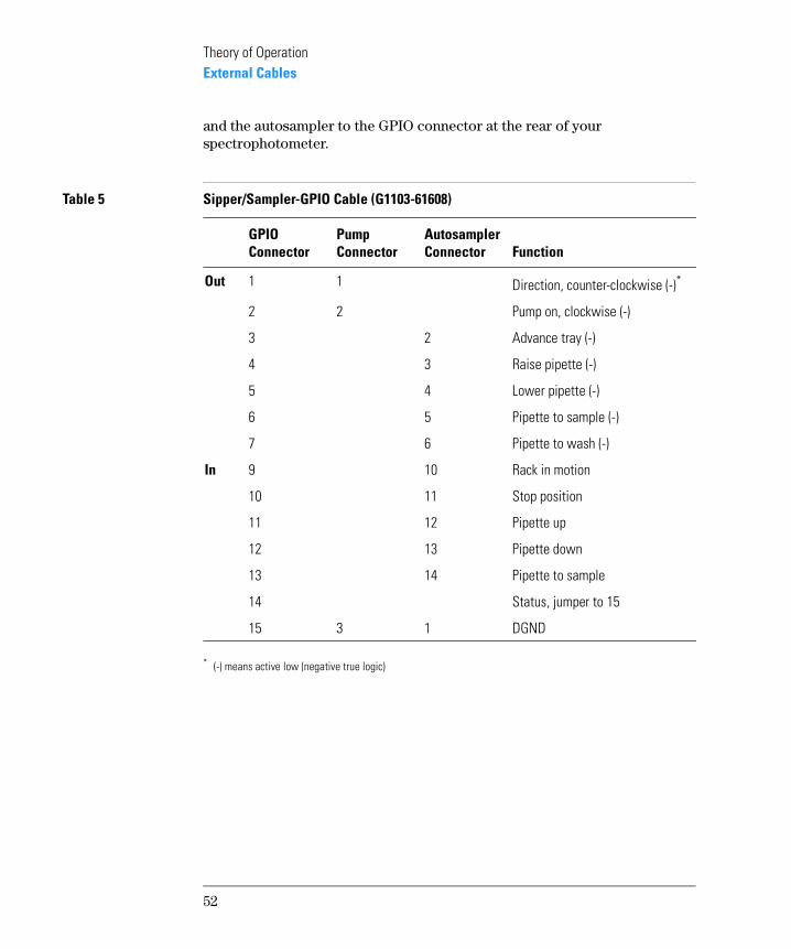
Theory of OperationExternal Cables
and the autosampler to the GPIO connector at the rear of your spectrophotometer.
Table 5 Sipper/Sampler-GPIO Cable (G1103-61608)
GPIO Connector
Pump Connector
Autosampler Connector Function
Out 1 1 Direction, counter-clockwise (-)*
2 2 Pump on, clockwise (-)
3 2 Advance tray (-)
4 3 Raise pipette (-)
5 4 Lower pipette (-)
6 5 Pipette to sample (-)
7 6 Pipette to wash (-)
In 9 10 Rack in motion
10 11 Stop position
11 12 Pipette up
12 13 Pipette down
13 14 Pipette to sample
14 Status, jumper to 15
15 3 1 DGND
* (-) means active low (negative true logic)
52

Theory of OperationExternal Cables
Multichannel Pump-GPIO Cable
The multichannel pump-GPIO cable (part number G1103-61607) is used to connect the 8-channel peristaltic pump to the GPIO connector at the rear panel of your spectrophotometer.
Table 6 Multichannel Pump Cable (G1103-61607)
GPIO Connector
Pump Connector Function
1 4 Direction, counter-clockwise (-)*
2 3 Pump on, clockwise (-)
14 Status, jumper to 15
15 1–2, connected DGND
* (-) means active low (negative true logic)
53

Theory of OperationExternal Cables
Valve Controller-GPIO Cable
The valve controller-GPIO cable (part number G1103-61610) is used to connect the valve/pump controller to the GPIO connector at the rear panel of your spectrophotometer.
General-Purpose-GPIO Cable
The general-purpose-GPIO cable (part number G1103-61611) has only a connector on the spectrophotometer side. It is used to connect any custom made device with parallel I/O to the GPIO connector at the rear panel of your spectrophotometer.
Table 7 Valve Controller-GPIO Cable (G1103-61610)
Valve Connector
GPIO Connector Function
Out 1 15 DGND
2 1 A0
3 2 A1
4 3 A2
5 9 D0IN
6 10 D1IN
7 11 D2IN
8 4 R/W(-)*
In 9 5 DV(-)
12 12 Rdy(-)
13 6 D0OUT
14 7 D1OUT
15 8 D2OUT
* (-) means active low (negative true logic)
54

Theory of OperationExternal Cables
Table 8 General Purpose Cable (G1103-61611)
Pin Function Pin Function
1 OUT [0] 9 IN [0]
2 OUT [1] 10 IN [1]
3 OUT [2] 11 IN [2]
4 OUT [3] 12 IN [3]
5 OUT [4] 13 IN [4]
6 OUT [5] 14 IN [5]
7 OUT [6] 15 DGND
8 OUT [7]
55
Theory of OperationExternal Connectors
External Connectors
GPIB Connector
The GPIB core design is used as talker/listener and a controller which is usually the computer with Agilent ChemStation software loaded. It supports all GPIB functionality except passing control between different devices. The connector needs to be activated and configured by the 8-bit configuration switch next to the GPIB connector. For switch settings, refer to the Installing Your UV-Visible Spectroscopy System handbook.
APG Remote Connector
Remote control allows easy connection between single instruments or systems to ensure coordinated analysis with simple coupling requirements.
A subminiature D connector is used. The module provides one remote connector which is inputs/outputs (wired-or technique).
To provide maximum safety within a distributed analysis system, one line is dedicated to SHUT DOWN the system’s critical parts in case any module detects a serious problem. To detect whether all participating modules are switched on or properly powered, one line is defined to summarize the POWER ON state of all connected modules. Control of analysis is maintained by signal readiness READY for next analysis, followed by START of run and optional STOP of run triggered on the respective lines. In addition PREPARE and START REQUEST may be issued.
Table 9 APG Remote Signal Distribution
Pin Signal Function
1 DGND Digital ground
2 PREPARE (L) Request to prepare for analysis (e.g. calibration, detector lamp on). Receiver is any module performing preanalysis activities.
3 START (L) Request to start run / timetable. Receiver is any module performing runtime controlled activities.
56

Theory of OperationExternal Connectors
Multicell Transport Connector
4 SHUT DOWN (L) System has serious problem. Receiver is any module capable to reduce safety risk.
5 Not used
6 POWER ON (H) All modules connected tosystem are switched on. Receiver is any module relying on operation of others.
7 READY (H) System is ready for next analysis. Receiver is any sequence controller.
8 STOP (L) Request to reach system ready state as soon as possible (e.g. stop run, abort or finish and stop injection). Receiver is any module performing runtime controlled activities.
9 START REQUEST (L) Request to start injection cycle (e.g. by start key on any module). Receiver is the autosampler.
Table 9 APG Remote Signal Distribution
Pin Signal Function
Table 10 Multicell Transport Connector
Pin Function Pin Function
1 Status 9 Limit switch (nc)
2 OUT [4] 10 Case
3 OUT [4] 11 OUT [2]
4 OUT [1] 12 OUT [2]
5 OUT [1] 13 OUT [3]
6 DGND 14 OUT [3]
7 DGND 15 Shield
8 Limit switch (no)
57

Theory of OperationExternal Connectors
CAN Connector
The CAN is a high speed communication interface. It is a two-wire serial bus system supporting data communication with realtime requirements. This CAN interface is used to connect the handheld controller of the Agilent 8453E UV-visible spectroscopy system to the spectrophotometer.
RS232C Connector
The RS232 is designed as DCE (Data Communication Equipment) with a 9 pin male SUB-D type connector. When controlling the spectrophotometer through the RS232 interface, the connector needs to be activated and configured by the 8-bit configuration switch next to the GPIB connector. For switch settings, refer to Chapter 6 “Interfacing”.
Using a serial/parallel printer cable, an HP printer can be connected to the spectrophotometer. This option is only used by the Agilent 8453E UV-visible spectroscopy system. The 8-bit configuration switch has to be set to GPIB communication and not to RS232 communication.
Table 11 RS232 Connector
Pin Function Pin Function
1 DCD 6 DSR
2 RxD 7 RTS
3 TxD 8 CTS
4 DTR 9 RI
5 GND
58
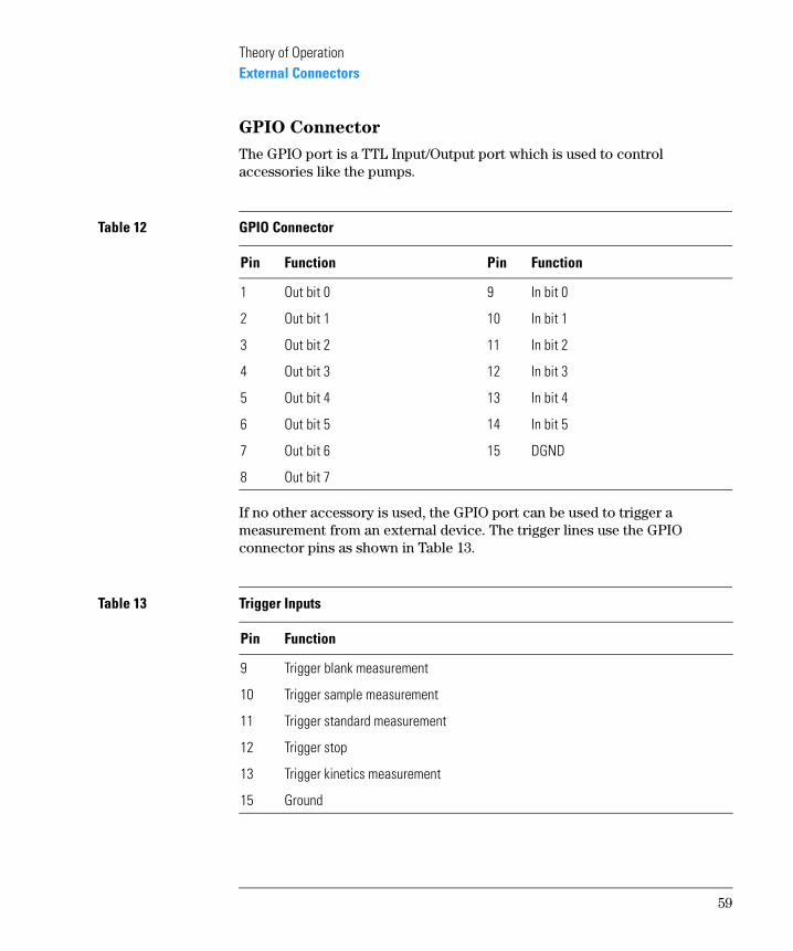
Theory of OperationExternal Connectors
GPIO Connector
The GPIO port is a TTL Input/Output port which is used to control accessories like the pumps.
If no other accessory is used, the GPIO port can be used to trigger a measurement from an external device. The trigger lines use the GPIO connector pins as shown in Table 13.
Table 12 GPIO Connector
Pin Function Pin Function
1 Out bit 0 9 In bit 0
2 Out bit 1 10 In bit 1
3 Out bit 2 11 In bit 2
4 Out bit 3 12 In bit 3
5 Out bit 4 13 In bit 4
6 Out bit 5 14 In bit 5
7 Out bit 6 15 DGND
8 Out bit 7
Table 13 Trigger Inputs
Pin Function
9 Trigger blank measurement
10 Trigger sample measurement
11 Trigger standard measurement
12 Trigger stop
13 Trigger kinetics measurement
15 Ground
59

Theory of OperationExternal Connectors
UV-vis ChemStation Software
Measurements are activated on contact closure to ground (pin 15). By default these trigger lines are inactive. To activate the GPIO lines as trigger lines, type the following command on the command line of the Agilent ChemStation:
EnableGPIOButtons 1
This activation is not resident and has to be done every time the ChemStation is started or the Agilent 8453 is switched on again.
The general purpose cable G1103-61611 is recommended for connecting external hardware devices to the GPIO interface of the spectrophotometer.
Handheld Controller Software
Measurements are activated on contact closure to ground (pin 15). By default these trigger lines are active.
Pin 12 (Trigger Stop) and Pin 13 (Trigger kinetics run) are not supported by the software of the handheld controller.
The general purpose cable G1103-61611 is recommended for connecting external hardware devices to the GPIO interface of the spectrophotometer.
60

Theory of OperationExternal Connectors
61

Internal Connections
This section gives the definition of the connections inside the instrument
including pin assignments of the connectors. Only those connectors are described which may be important for troubleshooting.62

Theory of OperationConnector Definitions
Connector Definitions
Main Power Supply Connector
The main power supply is connected to the spectrophotometer processor main (SPM) board by a cable that is fixed to the main power supply.
Fan Connector
The fan is connected to the spectrophotometer processor main (SPM) board.
Table 14 Power Supply Cable to SPM Board
Pin Function Pin Function
1 Power failure 7,8 +24 V
2 Analog ground (AGND) 9,10 +36 V (not used)
3 -15 V 11 Digital ground (DGND)
4 +15 V 12 +5 V
5,6 Power ground (PGND)
Table 15 Fan Connector
Pin Function
1 Fan Power
2 Fan Rotation Sensor
3 GND
63

Theory of OperationConnector Definitions
Shutter Assembly Connector
The shutter assembly is connected to the spectrophotometer processor main (SPM) board.
Deuterium Lamp Connector
The deuterium lamp is connected to the spectrograph lamp supply (SLS) board.
Table 16 Shutter Assembly Connector
Pin Function
1,2 Coil Filter
3,4 Coil Dark
5,6 GND
7,8 Coil Common
9,10 GND
Table 17 Deuterium Lamp Connector
Pin Function
1 Heater
2 Cathode
3 Anode
64

Theory of OperationConnector Definitions
Tungsten Lamp Connector
The tungsten lamp is connected to the spectrograph lamp supply (SLS) board.
Table 18 Tungsten Lamp Connector
Pin Function
1 Vis Sense +
2 Vis Lamp +
3 Vis Lamp -
4 Vis Sense -
65

Theory of OperationConnector Definitions
66

3
3 Diagnostics and
Troubleshooting
Explainations of status and error messages and a logical approach to troubleshooting

Diagnostics and
Troubleshooting
For different stages of troubleshooting, the startup test of the spectrophotometer, instrument self-test, and various diagnostic tests are used.
Instrument start-up tests are implemented in the spectrophotometer firmware. They are used to check if the instrument electronics are functioning during start up and operation of the instrument and create error messages or symptoms on the front panel status LEDs. Self-test and diagnostic tests are implemented in the operating software. For explanation of these tests, see your software documentation and online help in the software.
This chapter covers the following topics related to troubleshooting the spectrophotometer:
• front panel status and power switch LEDs,
• error messages, and
• general troubleshooting hints.
This chapter gives information about how to troubleshoot the instrument. For detailed procedures about cleaning lenses, disassembling the spectrophotometer and exchanging individual electronic items, see Chapter 4 “Maintenance and Repair”.
68

Diagnostics and TroubleshootingFront Panel Status and Power Switch LEDs
Front Panel Status and Power Switch
LEDs
A general description of the functionality of the status and power switch LEDs is given in Chapter 2 “Theory of Operation”. This section describes typical LED symptoms in case of failures of the instrument.
Power switch LED off The line power switch with the power switch LED is located at the lower left part of the instrument. If the line power switch is pressed in but the green light is off:
• the instrument may not be connected to line power, or
• the main power supply (MPS) is defective.
Refer to Table 20 through Table 34 for detailed troubleshooting information.
Red front panel LED The spectrophotometer does not pass one of the self-tests which are run when the spectrophotometer is turned on or an error occurred during operation. Most of the causes have to do with ignition of lamps, open lamp door, multicell transport problems or spectrophotometer hardware problems.
If your controller is running (personal computer or handheld controller) and connected to the spectrophotometer, you may get an error message. This message will tell you more about the cause of the error. For details about error messages, see Table 20 through Table 34 or the help system.
Red, blinking front panel LED
Error condition of the spectrophotometer processor system. Because in this case there is no communication with the computer there will be no error message. Turn the instrument off and on again. If the error appears again, possible causes are shown in Table 19.
69

Diagnostics and TroubleshootingFront Panel Status and Power Switch LEDs
Table 19 Error Condition of Spectrophotometer Processor System
Possible Causes Action
Spectrophotometer main processor (SPM) board defective
Exchange SPM board
Spectrophotometer data acquisition (SDA) board defective
Exchange SDA board
70

Diagnostics and TroubleshootingError Messages
Error Messages
Error messages are a series of text messages which appear in your software. These messages notify you that either the spectrophotometer is not functioning correctly or, in case you are using your own customized programs, that you have made a mistake in the commands which you have given to the spectrophotometer.
The following is an overview of the error messages. For suggestions regarding causes and courses of action, see Table 20 through Table 34.
• Multicell Transport Home Position Not Found
• No Filament Current On Deuterium Lamp
• Deuterium Lamp Ignition Failed
• No Current Sensed On Deuterium Lamp
• No Voltage Sensed On Deuterium Lamp
• No Current Sensed On Tungsten Lamp
• No Voltage Sensed On Tungsten Lamp
• Cooling Fan Defective
• Lamp Door Open (Lamps are switched off)
• Digital Signal Processor Error
• Wavelength Calibration Data Rejected
• Excessive Dark Current Detected On Photodiodes
• Raw Data Buffer Overflow
• Power Fail
Most of these error messages are stored with the Agilent 8453 spectrophotometer logbook and can be recalled through the operating software.
Table 20 through Table 34 show the error messages with their meanings. The tables explain the instrumental conditions required to generate the message and potential causes which lead to generation of the message. There is a list of suggested actions to correct the instrument state when necessary.
71

Diagnostics and TroubleshootingError Messages
Table 20 Multicell Transport Home Position Not Found
Possible Causes Action
The multicell transport mechanism is jammed.
Make sure the carriage can move freely along its entire path and that there are no obstructions
Check that the two screws which fix the multicell transport in the spectrophotometer are not pushed up into the path of the mechanism (e.g. this is the case when putting the transport beside the instrument).
Electronics failed. Check for defective HOME-switch, defective multicell transport cable, defective motor, or defective spectrophotometer processor main (SPM) board.
Table 21 Lamp Door Open (Lamps Are Switched Off)
Possible Causes Action
Lamp door is open. Close lamp door.
Lamp door is bent. Light switch tab is positioned incorrectly.
Bend light switch tab on lamp door to correct tab position.
Light switch or electronics have failed. Replace spectrophotometer lamp power supply (SLS) board.
72

Diagnostics and TroubleshootingError Messages
Table 22 Invalid Data Points In Spectrum
Possible Causes Action
Blank has higher absorbance than sample measurement. Solvent or chemical matrix of blank has higher absorbance than solvent/matrix of sample.
Ensure sample and blank use the same solvent or chemical matrix.
Measure blank on water.
In kinetics mode of ChemStation software:
1 Under Options & Information in the Method menu, select Adjust gains separately from blank measurement.
2 Under Set Gains in the Measure menu, select water or air
Bubble in flow cell absorbing during blank. Use cell cleaning fluid to prevent air bubbles sticking on the window surface of the flow cell.
Floating particle(s) in cell Clean cell or wait untill particle(s) have settled
Variation in sample absorbance during the measurement process due to chemical or physical processes.
Select a shorter integration time.
Fluorescent sample. Use fixed gain settings in your advanced software for the Agilent ChemStation.
This feature is not implemented in the software of the handheld controller.
Electronics failed. Replace the spectrophotometer data acquisition (SDA) board.
Replace optical unit.
Bad blank. Repeat blank measurement.
73
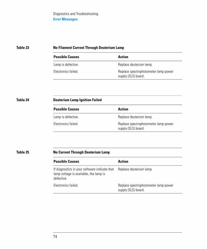
Diagnostics and TroubleshootingError Messages
Table 23 No Filament Current Through Deuterium Lamp
Possible Causes Action
Lamp is defective. Replace deuterium lamp.
Electronics failed. Replace spectrophotometer lamp power supply (SLS) board.
Table 24 Deuterium Lamp Ignition Failed
Possible Causes Action
Lamp is defective. Replace deuterium lamp.
Electronics failed. Replace spectrophotometer lamp power supply (SLS) board.
Table 25 No Current Through Deuterium Lamp
Possible Causes Action
If diagnostics in your software indicate that lamp voltage is available, the lamp is defective.
Replace deuterium lamp.
Electronics failed. Replace spectrophotometer lamp power supply (SLS) board.
74

Diagnostics and TroubleshootingError Messages
Table 26 No Voltage At Deuterium Lamp
Possible Causes Action
Lamp is defective. Replace deuterium lamp.
Electronics failed. Replace spectrophotometer lamp power supply (SLS) board.
Table 27 No Current Through Tungsten Lamp
Possible Causes Action
If diagnostics in your software indicate that lamp voltage is available, the lamp is defective.
Replace tungsten lamp.
Electronics failed. Replace spectrophotometer lamp power supply (SLS) board.
Table 28 No Voltage At Tungsten Lamp
Possible Causes Action
Lamp is defective. Replace tungsten lamp.
Electronics failed. Replace spectrophotometer lamp power supply (SLS) board.
75
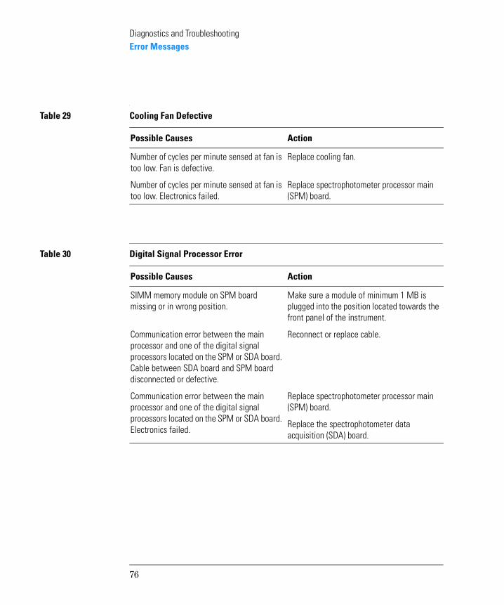
Diagnostics and TroubleshootingError Messages
Table 29 Cooling Fan Defective
Possible Causes Action
Number of cycles per minute sensed at fan is too low. Fan is defective.
Replace cooling fan.
Number of cycles per minute sensed at fan is too low. Electronics failed.
Replace spectrophotometer processor main (SPM) board.
Table 30 Digital Signal Processor Error
Possible Causes Action
SIMM memory module on SPM board missing or in wrong position.
Make sure a module of minimum 1 MB is plugged into the position located towards the front panel of the instrument.
Communication error between the main processor and one of the digital signal processors located on the SPM or SDA board. Cable between SDA board and SPM board disconnected or defective.
Reconnect or replace cable.
Communication error between the main processor and one of the digital signal processors located on the SPM or SDA board. Electronics failed.
Replace spectrophotometer processor main (SPM) board.
Replace the spectrophotometer data acquisition (SDA) board.
76
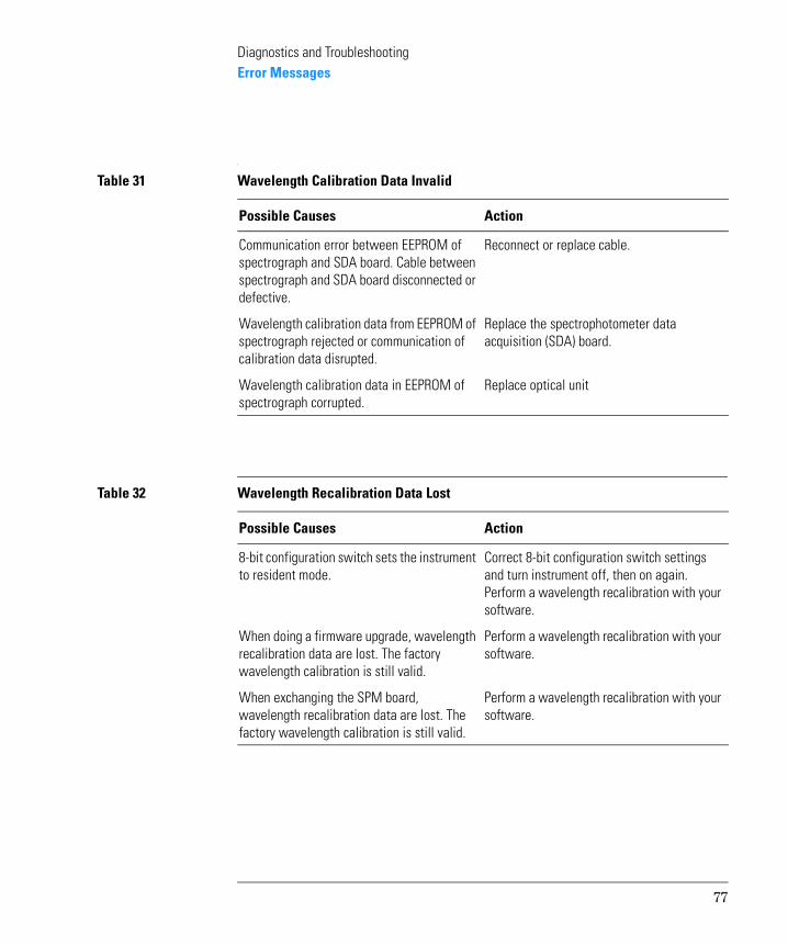
Diagnostics and TroubleshootingError Messages
Table 31 Wavelength Calibration Data Invalid
Possible Causes Action
Communication error between EEPROM of spectrograph and SDA board. Cable between spectrograph and SDA board disconnected or defective.
Reconnect or replace cable.
Wavelength calibration data from EEPROM of spectrograph rejected or communication of calibration data disrupted.
Replace the spectrophotometer data acquisition (SDA) board.
Wavelength calibration data in EEPROM of spectrograph corrupted.
Replace optical unit
Table 32 Wavelength Recalibration Data Lost
Possible Causes Action
8-bit configuration switch sets the instrument to resident mode.
Correct 8-bit configuration switch settings and turn instrument off, then on again. Perform a wavelength recalibration with your software.
When doing a firmware upgrade, wavelength recalibration data are lost. The factory wavelength calibration is still valid.
Perform a wavelength recalibration with your software.
When exchanging the SPM board, wavelength recalibration data are lost. The factory wavelength calibration is still valid.
Perform a wavelength recalibration with your software.
77

Diagnostics and TroubleshootingError Messages
Table 33 Excessive Dark Current Detected On Photodiodes
Possible Causes Action
Spectrophotometer data acquisition (SDA) board failure.
Replace spectrophotometer data acquisition (SDA) board.
Photodiode array electronics failure. Replace optical unit.
Table 34 Raw Data Buffer Overflow
Possible Cause Action
Attempting to acquire large amounts of data within too short of a time period.
Change data acquisition rate, and/or change cycle time, and/or change wavelength range.
78

Diagnostics and TroubleshootingError Messages
Table 35 Power Fail
Possible Causes Action
Instrument power fail. Check that instrument power indicator in on.
No interface link to PC Check that the GPIB cable is properly connected to both Agilent 8453 and PC.
Incorrect interface settings. Check that the GPIB interface setting on the spectrophotometer (see section “Installing your Agilent 8453 Spectrophotometer“ in the handbook Installing Your UV-visible Spectroscopy System), on the GPIB interface in PC (see section “Installing an GPIB Interface Board in the PC“ in the handbook Installing Your UV-visible Spectroscopy System), and in the software configuration (see section “Installing the UV-visible Operating Software“ in the handbook Installing Your UV-visible Spectroscopy System) are correct.
Loss of communication This may occur because of exceptional power line conditions (spikes or drop-outs). Check that the power supply to the instrument is good.
79

Diagnostics and TroubleshootingGeneral Troubleshooting Hints
General Troubleshooting Hints
Instrument problems may not always result in error messages. Proper instrument performance is determined by the quality of the results. Even if your instrument turns on, passes its self tests, and operates without generating error messages, it may not be functioning perfectly. The results of measurements can provide hints for troubleshooting if measurement results are less than optimal.
Typical power on sequence failed
During a typical power on sequence the following events occur:
• the power switch LED will ignite and remain on,
• the front panel LED will turn yellow, then flash red, green, and stay yellow,
• the fan speed will decrease,
• the shutter will close, if you listen carefully you may here a click,
• the front panel LED will turn green.
The green front panel LED indicates successful completion of the self test sequence.
NOTE Your software may be set so that lamp ignition does not automatically occur during power on. In this case use your software to ignite the deuterium and tungsten lamps.
80

Diagnostics and TroubleshootingGeneral Troubleshooting Hints
If any or all of the above listed actions do not occur, there may be a problem with your instrument. Refer to Table 36 through Table 41 for further troubleshooting information.
Table 36 Power Switch LED Off — Front Panel LED Off
Possible Causes Action
Instrument power disconnected. Connect instrument to power.
Overcurrent or overvoltage condition. Spring below optical unit may be bent. This may result in a short circuit on the SDA board.
Remove optical unit. Bend spring back and turn instrument off and on again to reset main power supply.
Overcurrent or overvoltage condition. Electronics failure.
Turn instrument off and on again to reset main power supply. If the error condition remains, disconnect internal boards one by one, repetitively turning the instrument off and on, to find the defective board.
Main power supply (MPS) defective. Replace main power supply (MPS).
Table 37 Power Switch LED Off — Front Panel LED On
Possible Cause Action
LED in main power supply (MPS) defective. Replace main power supply (MPS).
Table 38 Power Switch LED On — Front Panel LED Off — Shutter Clicks
Possible Causes Action
Front panel keyboard (SSI board) disconnected or cable defective.
Reconnect or replace cable.
Front panel keyboard (SSI board) defective. Replace front panel keyboard (SSI board).
81

Diagnostics and TroubleshootingGeneral Troubleshooting Hints
Table 39 Power Switch LED On — Front Panel LED Off — Shutter Does Not Click
Possible Causes Action
8-bit configuration switch sets the instrument to resident mode.
Correct 8-bit configuration switch settings and turn instrument off, then on again. Because the wavelength recalibration is lost, perform a wavelength recalibration with your software.
Spectrophotometer data acquisition (SDA) board disconnected or defective.
Connect or replace spectrophotometer data acquisition (SDA) board.
Main power supply (MPS) not connected to spectrophotometer processor main (SPM) board.
Connect main power supply (MPS) to spectrophotometer processor main (SPM) board.
Main power supply (MPS) or spectrophotometer processor main (SPM) board defective.
Replace main power supply (MPS) or spectrophotometer processor main (SPM) board.
Table 40 Power Switch LED Flickering — Front Panel LED Off — Shutter Does Not Click
Possible Cause Action
Main power supply (MPS) not connected to spectrophotometer processor main (SPM) board.
Connect main power supply (MPS) to spectrophotometer processor main (SPM) board.
82

Diagnostics and TroubleshootingGeneral Troubleshooting Hints
Table 41 Front Panel LED Red
Possible Cause Action
An appropriate error message should occur in your software. For explanation of error messages, see “Error Messages” on page 71.
Lamp door open or missing. Close or replace door.
Lamp door sensor defective. Replace spectrophotometer lamp power supply (SLS) board.
Shutter failed or disconnected. Connect or replace shutter.
Spectrograph disconnected or defective. Connect or replace spectrograph.
Spectrophotometer lamp power supply (SLS) board disconnected or defective.
Connect or replace spectrophotometer lamp power power supply (SLS) board.
83
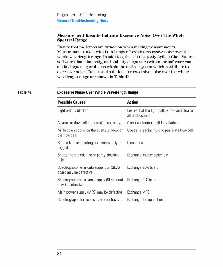
Diagnostics and TroubleshootingGeneral Troubleshooting Hints
Measurement Results Indicate Excessive Noise Over The Whole
Spectral Range
Ensure that the lamps are turned on when making measurements. Measurements taken with both lamps off exhibit excessive noise over the whole wavelength range. In addition, the self test (only Agilent ChemStation software), lamp intensity, and stability diagnostics within the software can aid in diagnosing problems within the optical system which contribute to excessive noise. Causes and solutions for excessive noise over the whole wavelength range are shown in Table 42.
Table 42 Excessive Noise Over Whole Wavelength Range
Possible Causes Action
Light path is blocked. Ensure that the light path is free and clear of all obstructions
Cuvette or flow cell not installed correctly. Check and correct cell installation.
Air bubble sticking on the quartz window of the flow cell.
Use cell cleaning fluid to passivate flow cell.
Source lens or spectrograph lenses dirty or fogged.
Clean lenses.
Shutter not functioning or partly blocking light.
Exchange shutter assembly.
Spectrophotometer data acqusition (SDA) board may be defective.
Exchange SDA board.
Spectrophotometer lamp supply (SLS) board may be defective.
Exchange SLS board.
Main power supply (MPS) may be defective. Exchange MPS.
Spectrograph electronics may be defective. Exchange the optical unit.
84

Diagnostics and TroubleshootingGeneral Troubleshooting Hints
Measurement Results Indicate Excessive Noise in Part of the
Spectrum
The selftest (only Agilent ChemStation software), lamp intensity, and stability diagnostics within the software can aid in diagnosing problems within the optical system which contribute to excessive noise. Low intensity in one wavelength range may not preclude you from using the spectrophotometer at another wavelength range where the intensity is acceptable. Causes and solutions for excessive noise in part of the spectrum are shown in Table 43.
Table 43 Excessive Noise in Part of Spectrum
Possible Causes Action
One of the lamps may be turned off when making measurements. Measurements taken with the deuterium lamp off exhibits excessive noise in the UV wavelength range. Measurements taken with the tungsten lamp off exhibits excessive noise in the visible wavelength range.
Switch on proper lamp.
Noise in the UV wavelength range may be caused by a weak or defective deuterium lamp.
Exchange the lamp. Lifetime of the deuterium lamp may be influenced by the number of ignitions.
Flow cells and cuvettes, which reduce and/or distort the colimated light beam used in the spectrophotometer, can result in low lamp intensity at the spectrograph.
Change cell to standard type. Glass absorbs in the low UV region and causes high noise. Make sure that your flow cells and cuvettes are made from quartz.
Solvent or buffer blocks light in a certain wavelength range.
If information is required in such a wavelength range, a solvent or buffer that is transparent in that range should be used.
Fingerprints on cuvettes or flow cells typically absorb light in the UV range of the spectrum.
Clean your flow cells or cuvettes with a lens cleaning tissue.
Source lens or spectrograph lenses dirty or fogged.
Clean lenses.
Spectrophotometer lamp supply (SLS) board may be defective.
Exchange SLS board.
85
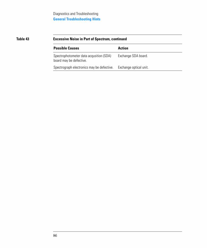
Diagnostics and TroubleshootingGeneral Troubleshooting Hints
Spectrophotometer data acqusition (SDA) board may be defective.
Exchange SDA board.
Spectrograph electronics may be defective. Exchange optical unit.
Table 43 Excessive Noise in Part of Spectrum, continued
Possible Causes Action
86

Diagnostics and TroubleshootingGeneral Troubleshooting Hints
Measurement Results Indicate Excessive Drift
The selftest (only Agilent ChemStation software), lamp intensity, and stability diagnostics within the software can aid in diagnosing problems within the optical system which contribute to excessive drift. Causes and solutions for excessive drift are shown in Table 44.
Table 44 Excessive Drift
Possible Causes Action
Variations in temperature. Ensure that the environment in which the spectrophotometer is being used is stable. The photodiode array temperature may be monitored from within the software to verify PDA temperature stability.
Sample degrades with time and/or exposure to light.
Use the spectrophotometer without sample. If the problem is found to be sample related, i.e. sample exposure to light, limit the amount of light by the environment and/or shorten the integration time to limit the amount of light during the measurement or use filter wheel to cut out the energetic low UV range.
Floating particles in the cell. Filter sample before measurement.
Deuterium lamp may burn unstable. Exchange lamp.
Tungsten lamp may burn unstable Exchange lamp.
Spectrophotometer lamp supply (SLS) board may supply unstable power.
Exchange SLS board.
Spectrophotometer data acqusition (SDA) board may be defective.
Exchange SDA board.
Main power supply (MPS) may supply unstable power.
Exchange MPS.
Spectrograph electronics may be defective. Exchange optical unit.
87

Diagnostics and TroubleshootingGeneral Troubleshooting Hints
Excessive Spikes or Glitches on Spectra
Causes and solutions for excessive spikes or glitches on spectra are shown in Table 45.
Table 45 Excessive Spikes or Glitches on Spectra
Possible Causes Action
BLANK on air, SAMPLE on cuvette. Measure Blank on the same solvent as used for the sample.
Dramatic changes in the refractive index from BLANK to SAMPLE.
Measure Blank on the same solvent as used for the sample.
Wedge shaped cuvettes (low quality cuvettes, mostly (not always) plastic cuvettes; there are non-wedge shaped plastic cuvettes available).
Use high quality quartz cuvettes.
Bubbles in the cell (even very small ones are sufficient to create spikes).
Try to get rid of the bubbles by gently knocking the cell on a desk. Rinsing the cells with a cleaning and pasivating solution makes the bubbles less sticky to the windows.
Sometimes the use of degassed solvent prevents the building of bubbles and make to time between filling the cells and the measurement as short as possible.
Floating particles in the cell (from cleaning tissues, or the application, or other kind of dirt).
Cells have to be cleaned using cleaning and pasivating solution. Use optical tissues to wipe the outer surface of the cells.
Any kind of addionally mounted optical devices put into the light path of the instrument.
The manipulation of the optical characteristics can cause some decrease in optical performance. No corrective action execpt the remove of the optical active device can change the behavior.
Turbid samples (especially in kinetics when a mixing process occurs during measurement).
Avoid turbidity, e.g. by filtration.
88

Diagnostics and TroubleshootingGeneral Troubleshooting Hints
Apertured cells For single cell holder:
For cells with apertures of 2 mm or smaller, always use flow cells and avoid removing it between measurements.
For multicell transport:
Never use a multicell transport as a single cell holder when apertured cuvettes are in use (BLANK on position number 1 and SAMPLE on all other positions) without doing a zero cells measurement.
Avoid removing and replacing the cells during a series of measurements.
Be sure that the clamp of the multicell (89075D) is always closed then doing a measurement.
In general use only cells with blackened walls.
Table 45 Excessive Spikes or Glitches on Spectra, continued
Possible Causes Action
89

Diagnostics and TroubleshootingGeneral Troubleshooting Hints
Excessive Stray Light or Nonlinearity
Causes and solutions for excessive stray light or nonlinearity are shown in Table 46.
Table 46 Excessive Stray Light or Nonlinearity
Possible Causes Action
Non-blackened apertured cells (so called flourescence cells or plastic cells)
Use only cells with blackened walls.
Weak intensity in the UV region of the spectrum.
Check Deuterium lamp intensity.
90

Diagnostics and TroubleshootingGeneral Troubleshooting Hints
Measurements are not Reproducible
Causes and solutions for measurements not being reproducible are shown in Table 47.
Table 47 Measurements are not Reproducible
Possible Causes Action
Very low sample concentration Increase integration time to improve signal-to-noise ratio.
Variations in the sample Check that the sample does not:
• contain particulates that float in and out of the light beam (filter if necessary)
• shows signs of bubble formation though chemical reaction or degassing
• show signs of thermal or photochemical degradation.
One lamp switched off Check that both lamps are switched on if measurement over whole spectral range is required. If spectra in the UV range only are being measured then deuterium lamp must be on. If spectra in the Visible range only are being measured then tungsten lamp must be on.
Weak lamp Use diagnostics intensity test to check if lamp intensity is too low and change lamp if necessary.
91

Diagnostics and TroubleshootingGeneral Troubleshooting Hints
Measured Values are Different to those of Another Instrument
Causes and solutions for measured values being different to those of another instrument are shown in Table 48.
Table 48 Measured Values are Different to those of Another Instrument
Possible Causes Action
Very low sample concentration Increase integration time to improve signal-to-noise ratio.
Variations in the sample Check that the sample does not:
• contain particulates that float in and out of the light beam (filter if necessary)
• shows signs of bubble formation though chemical reaction or degassing
• show signs of thermal or photochemical degradation.
One lamp switched off Check that both lamps are switched on if measurement over whole spectral range is required. If spectra in the UV range only are being measured then deuterium lamp must be on. If spectra in the Visible range only are being measured then tungsten lamp must be on.
Weak lamp Use diagnostics intensity test to check if lamp intensity is too low and change lamp if necessary.
92

4
4 Maintenance and Repair
Procedures for exchanging parts, such as lamps and electronic or mechanical items, and for cleaning lenses
Maintenance
This section describes maintenance procedures such as cleaning the
instrument, exchanging the deuterium and tungsten lamps and cleaning lenses. Always disconnect the instrument from line power before maintenance.WARNING To disconnect the instrument from line, pull out the power cord. The
power supply still uses some power, even if the power switch on the
front panel is turned off.
94

Maintenance and RepairCleaning the Instrument
Cleaning the Instrument
The spectrophotometer case and sample compartment should be kept clean. Cleaning should be done with a soft cloth slightly dampened with water or a solution of water and a mild detergent. Do not use an excessively damp cloth that liquid can drip into the spectrophotometer.
WARNING Do not let liquid drip into the instrument. It could cause shock hazard
and it could damage the instrument.
95

Maintenance and RepairExchanging the Deuterium or Tungsten Lamp
Exchanging the Deuterium or Tungsten
Lamp
You exchange the deuterium or the tungsten lamp when the intensity test, which is executed through your software, falls below the specified level or when one of the lamps no longert ignites.
Removing the Deuterium or Tungsten Lamp
1 Turn off the spectrophotometer and disconnect the power cord.
2 Open the plastic lamp door at the right side of the instrument.
Figure 11 Opening the Plastic Lamp Door
3 To open the metal door behind the plastic door, slide the lock mechanism down and simultaneously pull the door out.
96

Maintenance and RepairExchanging the Deuterium or Tungsten Lamp
Figure 12 Opening the Metal Lamp Door
4 Slide the metal door out to have access to the lamps.
WARNING The light emitted by the deuterium lamp in this instrument may cause
damage to the naked eye. Always turn off the deuterium lamp before
removing the deuterium lamp.
Figure 13 Sliding Out the Metal Lamp Door
5 To disconnect the lamp cables, press the plug which connects the tungsten or deuterium lamp to the printed circuit together on both sides and lift it up.
97

Maintenance and RepairExchanging the Deuterium or Tungsten Lamp
Figure 14 Disconnecting the Lamp Cables and Removing the Lamps
WARNING If you have been using the instrument, the lamp may be hot. Wait five
minutes until the lamp cools down.
Further, a hot lamp collects dust when taking it out. In case you reuse the lamp this dust would enter the optical system.
6 Use a Pozidriv screwdriver to open the two screws that hold each lamp and take it out holding it at the lamp ring.
7 Place the lamp(s) on a clean optical tissue or another place where it cannot collect dust.
CA UTIO N Never touch the quartz envelope of the deuterium lamp with your fingers. Fingerprints absorb UV light and may be burnt in, thus reducing lifetime of the lamp.
If you have accidentally touched it, use isopropanol to wipe the fingerprint off.
Deuterium lamp
Tungsten lamp
98
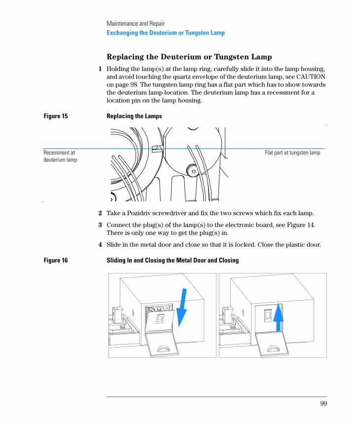
Maintenance and RepairExchanging the Deuterium or Tungsten Lamp
Replacing the Deuterium or Tungsten Lamp
1 Holding the lamp(s) at the lamp ring, carefully slide it into the lamp housing, and avoid touching the quartz envelope of the deuterium lamp, see CAUTION on page 98. The tungsten lamp ring has a flat part which has to show towards the deuterium lamp location. The deuterium lamp has a recessment for a location pin on the lamp housing.
Figure 15 Replacing the Lamps
2 Take a Pozidriv screwdriver and fix the two screws which fix each lamp.
3 Connect the plug(s) of the lamp(s) to the electronic board, see Figure 14. There is only one way to get the plug(s) in.
4 Slide in the metal door and close so that it is locked. Close the plastic door.
Figure 16 Sliding In and Closing the Metal Door and Closing
Recessment at deuterium lamp
Flat part at tungsten lamp
99

Maintenance and RepairExchanging the Deuterium or Tungsten Lamp
5 Reconnect line power and turn on the instrument. Check that the spectrophotometer passes its self-test, this means that the green light on the front panel comes on and that you can do a blank measurement from your software.
100

Maintenance and RepairCleaning the Stray Light Filter
Cleaning the Stray Light Filter
Cleaning the stray light filter is recommended at one-yearly intervals, or more frequently when you operate the spectrophotometer in particularly dirty environment. An indication for a dirty stray light filter is when
• —after exchanging the lamps—the intensity test executed by your operating software still falls below the specified level,
• one of the stray light tests fails,
• the photometric accuracy test fails.
Removing the Shutter Assembly
1 Turn off the spectrophotometer and disconnect the power cord. Take the plastic and sheet metal rear covers off, see “Removing and Replacing Covers” on page 109.
2 Remove any accessory board or MIO board that may be plugged in from the rear side of the instrument.
3 Remove the upper rear foam block
4 Disconnect the shutter cable from the SPM board. Open the screw that fixes the shutter assembly to the optical unit and remove the shutter assembly.
Figure 17 Removing the Shutter Assembly
Shutter assembly
Shutter screw
Stray light filter
101

Maintenance and RepairCleaning the Stray Light Filter
Cleaning the Stray Light Filter
1 Dampen a lint-free, surgical cotton swab with reagent grade isopropanol (isopropyl alcohol) and gently swab the surface of the stray light filter. Repeat several times with clean swabs and alcohol each time.
2 Use a canister of compressed oil-free air (like those used to clean photographic lenses) to further clean the stray light filter. If you do not have a compressed air canister, you can use a photographic lens cleaning brush.
Replacing the Shutter Assembly
1 Position the shutter assembly above the source lens and fix the screw that holds it at the optical unit, see Figure 39. Connect the shutter cable to the SPM board.
2 Replace the upper rear and upper front foam blocks.
3 If available, replace any accessory board or MIO board (plugged in from the rear side of the instrument).
4 Replace the plastic and sheet metal rear covers. Push the plastic rear cover down so that it locates on both sides, see “Removing and Replacing Covers” on page 109.
5 Reconnect line power and turn on the instrument. Check that the spectrophotometer passes its self-test, this means that the green light on the front panel comes on and that you can do a blank measurement from your software.
102

Maintenance and RepairCleaning the Lenses
Cleaning the Lenses
Cleaning the lenses which are accessible from the sample compartment is recommended at one-yearly intervals, or more frequently when you operate the spectrophotometer in a particularly dirty environment. An indication for dirty lenses is when—after exchanging the lamps—the intensity test executed by your operating software still falls below the specified level.
Cleaning the Source Lens
The source lens is a lens system which has one optical surface accessible from inside the lamp housing. The other optical surface is behind the shutter, thus accessible from the sample compartment.
Cleaning the Source Lens from the Sample Compartment Side
1 Turn-off the spectrophotometer and disconnect the power cord.
2 Remove any cuvette holder from the sample compartment.
3 To have better access you may want to take the plastic and metal rear covers off, see “Removing and Replacing Covers” on page 109.
4 Dampen a lint-free, surgical cotton swab with reagent grade isopropanol (isopropyl alcohol) and gently swab the surface of the source lens. Repeat several times with clean swabs and alcohol each time.
103

Maintenance and RepairCleaning the Lenses
Figure 18 Cleaning the Source Lens from the Sample Compartment Side
5 Use a canister of compressed oil-free air (like those used to clean photographic lenses) to further clean the source lens. If you do not have a compressed air canister, you can use a photographic lens cleaning brush.
6 If you have taken the covers off, replace them.
7 Replace the cuvette holder. Reconnect line power and turn on the instrument. Check that the spectrophotometer passes its self-test, this means that the green light on the front panel comes on and that you can do a blank measurement from your software.
Cleaning the Source Lens from the Lamp Side
It is not recommended to clean this lens at regular intervals, because the lamp housing is sealed against dust. Therefore the source lens is not very likely to get dirty from this side. However, if you have cleaned the other lenses and your intensity test in your operating software still falls below the specified level, try the procedure below.
1 Turn-off the spectrophotometer and disconnect the power cord.
2 To remove the Deuterium lamp, see “Exchanging the Deuterium or Tungsten Lamp” on page 96.
3 Dampen a lint-free, surgical cotton swab with reagent grade isopropanol (isopropyl alcohol) and gently swab the surface of the source lens. Repeat several times with clean swabs and alcohol each time.
Source lens
104

Maintenance and RepairCleaning the Lenses
Figure 19 Cleaning the Source Lens from the Lamp Side
4 Use a canister of compressed oil-free air (like those used to clean photographic lenses) to further clean the source lens. If you do not have a compressed air canister, you can use a photographic lens cleaning brush.
5 To replace the Deuterium lamp, see “Exchanging the Deuterium or Tungsten Lamp” on page 96.
6 Reconnect line power and turn on the instrument. Check that the spectrophotometer passes its self-test, this means that the green light on the front panel comes on and that you can do a blank measurement from your software.
Cleaning the Spectrograph Lens
1 Turn off the spectrophotometer and disconnect the power cord.
2 Remove any cuvette holder from the sample compartment.
3 To have better access you may want to take the plastic and metal front covers off, see “Removing and Replacing Covers” on page 109.
4 Dampen a lint-free, surgical cotton swab with reagent grade isopropanol (isopropyl alcohol) and gently swab the surface of the spectrograph lens. Repeat several times with clean swabs and alcohol each time.
Source lens
105

Maintenance and RepairCleaning the Lenses
Figure 20 Cleaning the Spectrograph Lens
5 Use a canister of compressed oil-free air (like those used to clean photographic lenses) to further clean the spectrograph lens. If you do not have a compressed air canister, you can use a photographic lens cleaning brush.
6 If you have taken the covers off, replace them. Replace the cell holder in the sample compartment.
7 Reconnect line power and turn on the instrument. Check that the spectrophotometer passes its self-test, this means that the green light on the front panel comes on and that you can do a blank measurement from your software.
Spectrograph lens
106

Maintenance and RepairCleaning the Lenses
107
Repair Procedures
This section gives detailed descriptions of procedures to repair the
instrument. Always disconnect the instrument from line power before repair.WARNING To disconnect the instrument from line, pull out the power cord. The
power supply still uses some power, even if the power switch on the
front panel is turned off.
For exchange of electronic assemblies we recommend to use an antistatic grounding kit (part number 9300-0933) to prevent the electronics from damage by electrostatic discharge.
• Before you unpack any electronic replacement parts, connect yourself electrically to the instrument with the help of a wrist strap.
• Connect the packing material with the electronic replacement part to the instrument.
• Touch electronic boards only on the corners and avoid touching the metal traces and electronic items on the board.
• When you remove electronic assemblies from the instrument, always put them back into the antistatic bags or place them on a material that has an electrical connection to the instrument.
108
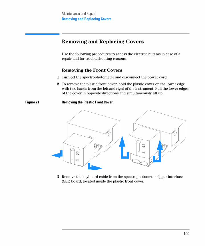
Maintenance and RepairRemoving and Replacing Covers
Removing and Replacing Covers
Use the following procedures to access the electronic items in case of a repair and for troubleshooting reasons.
Removing the Front Covers
1 Turn off the spectrophotometer and disconnect the power cord.
2 To remove the plastic front cover, hold the plastic cover on the lower edge with two hands from the left and right of the instrument. Pull the lower edges of the cover in opposite directions and simultaneously lift up.
Figure 21 Removing the Plastic Front Cover
3 Remove the keyboard cable from the spectrophotometer-sipper interface (SSI) board, located inside the plastic front cover.
109

Maintenance and RepairRemoving and Replacing Covers
Figure 22 Removing the Keyboard Cable
4 Remove the cuvette holder and sample pan from the sample compartment.
Figure 23 Removing Cuvette Holder and Sample Pan
5 To remove the sheet metal front cover, untighten the screw near the top of the cover using a Pozidriv screwdriver.
110

Maintenance and RepairRemoving and Replacing Covers
Figure 24 Removing the Sheet Metal Front Cover
6 Slide the sheet metal front cover towards the rear of the instrument and lift it up.
Replacing the Front Covers
1 Slide in metal front cover so that it locates on the bottom first. Slide it in further so that it locates on top.
Figure 25 Replacing the Metal Front Cover
2 Tighten the screw near the top of the cover using a Pozidriv screwdriver.
3 Replace the sample pan and cuvette holder in the sample compartment.
111

Maintenance and RepairRemoving and Replacing Covers
Figure 26 Replacing the Sample Pan and Cuvette Holder
4 Place the plastic front cover on top of the sheet metal cover so that you are able to connect the cable to the keyboard (SSI board).
Figure 27 Connecting the Keyboard Cable
5 Push the plastic cover down so that it locates on both sides.
6 Reconnect line power and turn on the instrument. Check that the spectrophotometer passes its self-test, this means that the green light on the front panel comes on and that you can do a blank measurement from your software and the keyboard of the spectrophotometer.
112

Maintenance and RepairRemoving and Replacing Covers
Removing the Rear Covers
1 Turn off the spectrophotometer and disconnect the power cord.
2 To remove the plastic rear cover, hold the plastic cover on the lower edge with two hands from the left and right of the instrument. Pull the lower edges of the cover in opposite directions and simultaneously lift up.
Figure 28 Removing the Plastic Rear Cover
3 Remove the cuvette holder and sample pan from the sample compartment.
Figure 29 Removing Cuvette Holder and Sample Pan
4 To remove the sheet metal rear cover, untighten the screw near the top of the cover using a Pozidriv screwdriver.
113

Maintenance and RepairRemoving and Replacing Covers
Figure 30 Removing the Sheet Metal Rear Cover
5 Slide the sheet metal rear cover towards the front of the instrument and lift it up.
Replacing the Rear Cover
1 Slide in metal rear cover so that it locates on the bottom first. Slide it in further so that it locates on top.
Figure 31 Replacing the Metal Rear Cover
2 Tighten the screw near the top of the cover using a Pozidriv screwdriver.
3 Replace the sample pan and cuvette holder in the sample compartment.
114

Maintenance and RepairRemoving and Replacing Covers
Figure 32 Replacing Sample Pan and Cuvette Holder
4 Replace the plastic cover and push it down so that it locates on both sides.
5 Reconnect line power and turn on the instrument. Check that the spectrophotometer passes its self-test, this means that the green light on the front panel comes on and that you can do a blank measurement from your software.
115
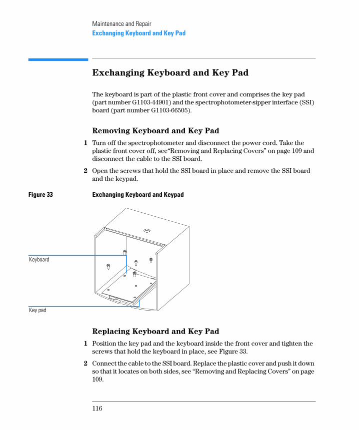
Maintenance and RepairExchanging Keyboard and Key Pad
Exchanging Keyboard and Key Pad
The keyboard is part of the plastic front cover and comprises the key pad (part number G1103-44901) and the spectrophotometer-sipper interface (SSI) board (part number G1103-66505).
Removing Keyboard and Key Pad
1 Turn off the spectrophotometer and disconnect the power cord. Take the plastic front cover off, see“Removing and Replacing Covers” on page 109 and disconnect the cable to the SSI board.
2 Open the screws that hold the SSI board in place and remove the SSI board and the keypad.
Figure 33 Exchanging Keyboard and Keypad
Replacing Keyboard and Key Pad
1 Position the key pad and the keyboard inside the front cover and tighten the screws that hold the keyboard in place, see Figure 33.
2 Connect the cable to the SSI board. Replace the plastic cover and push it down so that it locates on both sides, see “Removing and Replacing Covers” on page 109.
Key pad
Keyboard
116

Maintenance and RepairExchanging Keyboard and Key Pad
3 Reconnect line power and turn on the instrument. Check that the spectrophotometer passes its self-test, this means that the green light on the front panel comes on and that you can do a blank measurement from your software and the keyboard of the spectrophotometer.
117

Maintenance and RepairExchanging or Upgrading Internal Memory
Exchanging or Upgrading Internal Memory
Additional memory can be used in the spectrophotometer in case of very fast repetitive measurements of huge amounts of spectra, e.g. for fast kinetics measurements. Two sizes of memory are available, 1 MByte memory (part number 1818-4271) and 4 Mbyte memory (part number 1818-5784).
You can use the following combinations of memory modules: 1 × 1 MByte, 2 × 2 MByte, 1 × 4 MByte or 2 × 4 MByte.
Use the following procedure for removing and replacing memory.
Removing SIMM Memory Modules
1 Turn off the spectrophotometer and disconnect the power cord. Take the plastic and sheet metal rear covers off, see “Removing and Replacing Covers” on page 109.
2 Remove any accessory board or MIO board that may be plugged in from the rear side of the instrument.
Figure 34 Removing MIO or Accessory Boards
3 Remove the upper rear foam block.
4 On the two sides of the SIMM socket, move the two springs in opposite directions that the memory module is released and you can move the memory module towards the rear of the spectrophotometer..
118

Maintenance and RepairExchanging or Upgrading Internal Memory
Figure 35 Removing SIMM Memory Modules
5 Remove the memory module and repeat the last step in case there is a second memory module installed.
Replacing SIMM Memory Modules
1 Place the memory module in the SIMM socket on the SPM board that the components of the memory module are facing to the rear of the spectrophotometer. The memory module is now positioned at an angle in the SIMM socket.
2 Press the memory module towards the front of the spectrophotometer that it snaps in behind the two springs on either side of the SIMM socket.
3 Replace the upper rear foam block.
4 If available, replace any accessory board or MIO board (plugged in from the rear side of the instrument).
5 Replace the plastic and sheet metal rear cover. Push the plastic rear cover down so that it locates on both sides, see “Removing and Replacing Covers” on page 109.
6 Reconnect line power and turn on the instrument. Check that the spectrophotometer passes its self-test,this means that the green light on the front panel comes on and that you can do a blank measurement from your software.
SIMM memory modules
119
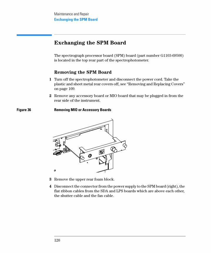
Maintenance and RepairExchanging the SPM Board
Exchanging the SPM Board
The spectrograph processor board (SPM) board (part number G1103-69500) is located in the top rear part of the spectrophotometer.
Removing the SPM Board
1 Turn off the spectrophotometer and disconnect the power cord. Take the plastic and sheet metal rear covers off, see “Removing and Replacing Covers” on page 109.
2 Remove any accessory board or MIO board that may be plugged in from the rear side of the instrument.
Figure 36 Removing MIO or Accessory Boards
3 Remove the upper rear foam block.
4 Disconnect the connector from the power supply to the SPM board (right), the flat ribbon cables from the SDA and LPS boards which are above each other, the shutter cable and the fan cable.
120

Maintenance and RepairExchanging the SPM Board
Figure 37 Removing Connectors and Screws from SPM Board
5 Unscrew two screws each, at the GPIB connector, at the APG remote connector and at the multicell connector and remove the SPM board.
Replacing the SPM Board
1 Position the SPM board on the middle rear foam block.
2 Connect the connector from the power supply to the SPM board (right), the flat ribbon cables from the SDA and LPS boards which are above each other, the shutter cable and the fan cable, see Figure 37.
3 Fix two screws each, at the GPIB connector, at the APG remote connector and at the multicell connector.
4 Replace the upper rear foam block.
5 If available, replace any accessory board or MIO board (plugged in from the rear side of the instrument).
6 Replace the plastic and sheet metal rear cover. Push the plastic rear cover down so that it locates on both sides, see “Removing and Replacing Covers” on page 109.
7 Reconnect line power and turn on the instrument. Check that the spectrophotometer passes its self-test, this means that the green light on the front panel comes on and that you can do a blank measurement from your software.
SPM board
121

Maintenance and RepairExchanging the Optical Unit
Exchanging the Optical Unit
The optical unit (part number G1103-69002) includes spectrograph, optics bench, shutter and lamp housing and it is exchanged as one item.
Removing the Optical Unit
1 Turn off the spectrophotometer and disconnect the power cord. Take the plastic and sheet metal rear and front covers off, see “Removing and Replacing Covers” on page 109.
2 Remove any accessory board or MIO board that may be plugged in from the rear side of the instrument.
3 Remove the upper rear and upper front foam blocks.
4 Remove the Deuterium and Tungsten lamps, see “Exchanging the Deuterium or Tungsten Lamp” on page 96.
5 Disconnect the shutter cable from the SPM board and the flat ribbon cable from the spectrograph.
Figure 38 Removing the Optical Unit
6 Remove the three hexagonal screws that hold the optical unit on the chassis of the instrument. Take the screws out to be able to lift up the optical unit.
7 Lift the optical unit out of the instrument and place it on the bench.
122

Maintenance and RepairExchanging the Optical Unit
Replacing the Optical Unit
1 Place the optical unit onto the bottom chassis of the instrument. Tighten the three hexagonal screws that hold the optical unit on the chassis of the instrument, see Figure 38.
2 Connect the shutter cable to the SPM board and the flat ribbon cable to the spectrograph, see Figure 38.
3 Replace the deuterium and tungsten lamps, see “Exchanging the Deuterium or Tungsten Lamp” on page 96.
4 Replace the upper rear and upper front foam blocks.
5 If available, replace any accessory board or MIO board (plugged in from the rear side of the instrument).
6 Replace the plastic and sheet metal front and rear covers. Push the plastic front and rear covers down so that they locate on both sides, see “Removing and Replacing Covers” on page 109.
7 Reconnect line power and turn on the instrument. Check that the spectrophotometer passes its self-test, this means that the green light on the front panel comes on and that you can do a blank measurement from your software.
123

Maintenance and RepairExchanging the Shutter Assembly
Exchanging the Shutter Assembly
The shutter assembly (part number G1103-61904) is located in the top rear part of the spectrophotometer.
Removing the Shutter Assembly
1 Turn off the spectrophotometer and disconnect the power cord. Take the plastic and sheet metal rear covers off, see “Removing and Replacing Covers” on page 109.
2 Remove any accessory board or MIO board that may be plugged in from the rear side of the instrument.
3 Remove the upper rear foam block
4 Disconnect the shutter cable from the SPM board. Open the screw that fixes the shutter assembly to the optical unit and remove the shutter assembly.
Figure 39 Removing the Shutter Assembly
Shutter assembly
Shutter screw
124

Maintenance and RepairExchanging the Shutter Assembly
Replacing the Shutter Assembly
1 Position the shutter assembly above the source lens and fix the screw that holds it at the optical unit, see Figure 39. Connect the shutter cable to the SPM board.
2 Replace the upper rear and upper front foam blocks.
3 If available, replace any accessory board or MIO board (plugged in from the rear side of the instrument).
4 Replace the plastic and sheet metal rear covers. Push the plastic rear cover down so that it locates on both sides, see “Removing and Replacing Covers” on page 109.
5 Reconnect line power and turn on the instrument. Check that the spectrophotometer passes its self-test, this means that the green light on the front panel comes on and that you can do a blank measurement from your software.
125

Maintenance and RepairExchanging the Fan Assembly
Exchanging the Fan Assembly
The fan assembly (part number 3160-1103) is located in the top rear part of the spectrophotometer.
Removing the Fan Assembly
1 Turn off the spectrophotometer and disconnect the power cord. Take the plastic and sheet metal rear covers off, see “Removing and Replacing Covers” on page 109.
2 Remove any accessory board or MIO board that may be plugged in from the rear side of the instrument.
3 Remove the upper rear foam block.
4 Disconnect the fan cable from the SPM board and remove the fan assembly.
Figure 40 Removing the Fan Assembly
Replacing the Fan Assembly
1 Position the fan assembly in its recessment in the middle rear foam block and connect the fan cable to the SPM board.
2 Replace the upper rear and upper front foam blocks.
3 If available, replace any accessory board or MIO board (plugged in from the rear side of the instrument).
Fan assembly
126

Maintenance and RepairExchanging the Fan Assembly
4 Replace the plastic and sheet metal rear cover. Push the plastic rear cover down so that it locates on both sides, see “Removing and Replacing Covers” on page 109.
5 Reconnect line power and turn on the instrument. Check that the spectrophotometer passes its self-test, this means that the green light on the front panel comes on and that you can do a blank measurement from your software.
127

Maintenance and RepairExchanging SDA Board
Exchanging SDA Board
The SDA board (part number G1103-69504) is located below the optical unit of the spectrophotometer.
Removing the SDA Board
1 Turn off the spectrophotometer and disconnect the power cord. Take the plastic and sheet metal front and rear covers off, see “Removing and Replacing Covers” on page 109.
2 To remove the optical unit, see “Removing the Optical Unit” on page 122.
3 Remove the lower front foam block.
4 Disconnect the three cables from the SDA board and remove the five scews that hold the board in place.
Figure 41 Removing the SDA Board
SDA board
128

Maintenance and RepairExchanging SDA Board
Replacing the SDA Board
1 Position the SDA board on the bottom chassis of the instrument and fix the three scews that hold the board in place.
2 Connect the three cables to the SDA board, see Figure 41.
3 On the side which is near the front of the instrument, feed the broader cable through the hole in the lower front foam block and place the foam block on the chassis of the instrument.
Figure 42 Replacing SDA Board and Cables
4 To replace the optical unit, see “Replacing the Optical Unit” on page 123.
5 Replace the plastic and sheet metal rear cover. Push the plastic rear cover down so that it locates on both sides, see “Removing and Replacing Covers” on page 109.
6 Reconnect line power and turn on the instrument. Check that the spectrophotometer passes its self-test, this means that the green light on the front panel comes on and that you can do a blank measurement from your software.
Hole in foam block
Lower front foam block
SDA board
129

Maintenance and RepairExchanging SLS Board
Exchanging SLS Board
The SLS board (part number G1103-69502) is located below the SPM board in the rear part of the spectrophotometer.
Removing the SLS Board
1 Turn off the spectrophotometer and disconnect the power cord. Take the plastic and sheet metal front and rear covers off, see “Removing and Replacing Covers” on page 109.
2 To remove the optical unit, see “Removing the Optical Unit” on page 122.
3 To remove the fan, see “Removing the Fan Assembly” on page 126.
4 To remove the SPM board, see “Removing the SPM Board” on page 120.
5 Remove the middle rear foam block.
Figure 43 Removing the Middle Rear Foam Block
6 To slide the SLS board out of the tab on the right side, lift up the SLS board on the left side a little and slide it to the left.
middle rear foam
130

Maintenance and RepairExchanging SLS Board
Figure 44 Removing the SLS Board
Replacing the SLS Board
1 Slide the SLS board into the tab on the right side and push it down, see figure above.
2 Connect the flat ribbon cable that leads to the SPM board.
3 Replace the middle rear foam block.
Figure 45 Replacing the Middle Rear Foam Block
Tab to hold SLS board
SLS board
131
Maintenance and RepairExchanging SLS Board
4 To replace the SPM board, see “Replacing the SPM Board” on page 121.
5 To replace the fan, see “Replacing the Fan Assembly” on page 126.
6 To replace the optical unit, see on page 123.
7 Replace the plastic and sheet metal rear cover. Push the plastic rear cover down so that it locates on both sides, see “Removing and Replacing Covers” on page 109.
8 Reconnect line power and turn on the instrument. Check that the spectrophotometer passes its self-test, this means that the green light on the front panel comes on and that you can do a blank measurement from your software.
132

Maintenance and RepairExchanging the Main Power Supply
Exchanging the Main Power Supply
The main power supply (MPS) (part number 0950-2528) is located below the SPM board in the rear part of the spectrophotometer.
The main power supply (MPS) is in a separate housing. It does not contain any servicable parts inside. In case it is defective, it must not be opened but has to be exchanged as a complete assembly.
Removing the Main Power Supply
1 Turn off the spectrophotometer and disconnect the power cord. Take the plastic and sheet metal front and rear covers off, see “Removing and Replacing Covers” on page 109.
2 To remove the fan, see “Removing the Fan Assembly” on page 126.
3 To remove the SPM board, see “Removing the SPM Board” on page 120.
4 Remove the middle rear foam block.
Figure 46 Removing the Middle Rear Foam Block
5 To remove the light pipe, take the snap mechanism between two fingers and press it together to release the light pipe from the coupler on the main power supply. Remove the light pipe with the power button.
middle rear foam
133

Maintenance and RepairExchanging the Main Power Supply
Figure 47 Removing the Light Pipe
6 Open the two screws from the rear panel of the instrument that hold the main power supply in place and slide the main power supply out.
Figure 48 Removing the Main Power Supply Screws
Replacing the Main Power Supply
1 Place the main power supply on the bottom foam in the rear part of the instrument and fix the two screws from the rear panel of the instrument that hold the main power supply in place, see figure above.
2 Attach the power button to the light pipe and slide the light pipe with the power button into the hole of the bottom foam part that the power button comes out of the hole at the base of the instrument.
Light pipe
134
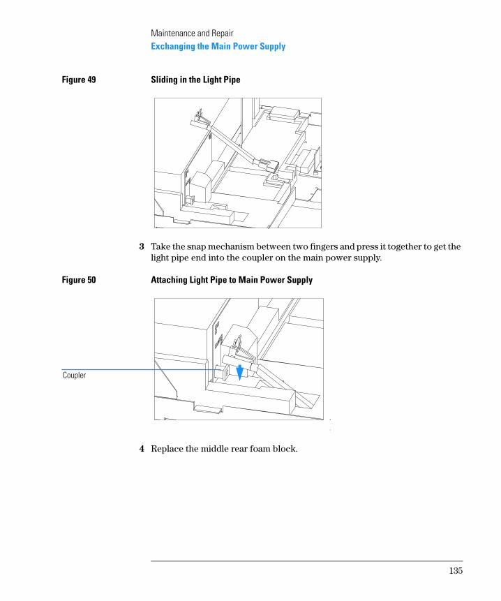
Maintenance and RepairExchanging the Main Power Supply
Figure 49 Sliding in the Light Pipe
3 Take the snap mechanism between two fingers and press it together to get the light pipe end into the coupler on the main power supply.
Figure 50 Attaching Light Pipe to Main Power Supply
4 Replace the middle rear foam block.
Coupler
135

Maintenance and RepairExchanging the Main Power Supply
Figure 51 Replacing the Middle Rear Foam Block
5 To replace the SPM board, see “Replacing the SPM Board” on page 121.
6 To replace the fan, see “Replacing the Fan Assembly” on page 126.
7 Replace the plastic and sheet metal rear cover. Push the plastic rear cover down so that it locates on both sides, see “Removing and Replacing Covers” on page 109.
8 Reconnect line power and turn on the instrument. Check that the spectrophotometer passes its self-test, this means that the green light on the front panel comes on and that you can do a blank measurement from your software.
136

5
5 Parts and Materials
Exploded views of repairable parts and part number listings for ordering replacement and exchange parts

Parts and MaterialsExploded Views and Part List
Exploded Views and Part List
Parts are listed in the respective tables with their part numbers. Assemblies shown do not contain any parts around them, unless otherwise specified.
Figure 52 Spectrophotometer Upper Parts
1 — inside parts shown in detail on next pages
2
3
7
811
4
6
9
5
14
16
15
12
13
10
25
27
138

Parts and MaterialsExploded Views and Part List
Table 49 Instrument Parts Breakdown
Item Description Part Number
1 Plastic cover front G1103-44101
2 Plastic cover rear G1103-68706
Name plate (not shown in Figure 52) G1103-44300
3, 4, 5 Sheet metal kit, containing:Metal top front, metal top rear, metal lamp door,(chassis bottom is included and shown in Figure 53)
G1103-68701
Metal cover screw (not shown in Figure 52) 5022-2112
5 Metal lamp door G1103-00301
6, 7, 16 EPP foam parts kit, containing:Foam front top, foam rear top, foam rear middle, (foam front bottom and foam rear bottom are included and shown in Figure 53)
G1103-68702
8 Sample pan G1103-44501
9 SPM board (spectr. proccessor main board) G1103-69500
10 Tungsten lamp G1103-60001
11 Screw M8 × 30 mm 0515-2520
12 Shutter assembly G1103-61904
13 1 MB memory for SPM board 1818-4721*
13 4 MB memory for SPM board 1818-5784**
14 Deuterium lamp 2140-0605
15 Optical unit (including spectrograph, optical bench and shutter) G1103-69002
* Part number may be subject to change.** Part number may be subject to change.
139

Parts and MaterialsExploded Views and Part List
Figure 53 Spectrophotometer Lower Parts
17, 19
34
21
23
29
31
36
35
18
32
30
28
33
20, 22, 24, 26
140

Parts and MaterialsExploded Views and Part List
Table 50 Instrument Parts Breakdown
Item Description Part Number
17 Power switch coupler 5041-8383
18 Fan assembly 3160-1103
19 PWR switch light pipe G1103-44602
20 Accessory slot cover 5001-3772
21 Power push button 5041-8381
22 GPIB standoff, 0.255 inch (not shown in Figure 53) 0380-0643
Washer (not shown in Figure 53) 3050-0893
23 Screw M3 × 8 mm 0515-1105
24 Remote standoff (not shown in Figure 53) 1251-7788
25, 27, 34, 36
Cable assembly kit G1103-68704
26 Screw set (not shown in Figure 53) 1251-0218
28 Screw M4 x 8 mm 0515-0910
Washer (not shown in Figure 53) 2190-0409
29, 32 EPP foam parts kit, containing:foam front bottom, foam rear bottom, (foam front top, foam rear top, foam rear middle are included and shown in Figure 52)
G1103-68702
30 Main power supply 0950-2528
31 SDA board (spectr. data acquisition board) G1103-69504
33 Sheet metal kit, containing:chassis bottom, (metal top front, metal top rear, metal lamp door are included and shown in Figure 52)
G1103-68701
Metal cover screw (not shown in Figure 53) 5022-2112
35 SLS board (spectr. lamp supply board) G1103-69502
141

Parts and MaterialsExploded Views and Part List
Figure 54 Front Cover Parts
Table 51 Front Cover Parts Breakdown
Item Description Part Number
37 Plastic Cover Front G1103-44101
38 Tapping Screw 0515-2734
39 SSI Board G1103-66505
40 Key Pad G1103-44901
37
38
39
40
142

Parts and MaterialsExploded Views and Part List
Parts not shown in the illustrated parts breakdown are given in Table 52.
Table 52 Additional Parts
Description Part Number
Standard cell holder 08451-60104
Sipper/sampler-GPIO cable G1103-61608
Multichannel pump-GPIO cable G1103-61607
Controller-GPIO cable G1103-61610
General purpose-GPIO cable G1103-61611
Waste tubing 0890-1711
GPIB cable (1m) 10833A
APG remote cable (start, stop, error, ready,shut down, power on)
5061-3378
Handheld controller with flexible CAN interface cable and documentation
G1819A
143

Parts and MaterialsExploded Views and Part List
144

6
6 Interfacing
Communicating and interfacing through GPIB and RS-232C

InterfacingSetting the 8-Bit Configuration Switch
Setting the 8-Bit Configuration Switch
The 8-bit configuration switch is located next to the GPIB connector. Switch settings provide configuration parameters for GPIB address, serial comunication protocol and instrument specific initialization procedures
Figure 55 8-Bit Configuration Switch.
If you just want to change the GPIB address and need a detailed procedure, refer to the Installing Your UV-Visible Spectroscopy System handbook. Default GPIB address is set to 25 equal to a binary setting of 0 0 0 1 1 0 0 1 (where 0 means that the switch is down and 1 means that the switch is up; the binary code of the address starts with the least significant bit at switch number 8).
Switches 1 and 2 define which set of parameters (for example, for GPIB, RS232 and so on) will be changed. Once the change has been completed, the instrument must be powered up again in order to store the values in the non-volatile memory.
In the non-volatile random access memory (NVRAM) the parameters are kept, independantly if you turn the instrument off and on again. They will be kept until the same set of parameters is subsequently changed and power is
1 2 3 4 5 6 7 8
Table 53 8-Bit Configuration Switch
Mode Select 1 2 3 4 5 6 7 8
GPIB 0 0 GPIB Address
RS-232 0 1 Baudrate Data Bits Parity
Reserved 1 0 Reserved
TEST/BOOT 1 1 RSVD SYS RSVD RSVD FC
146

InterfacingSetting the 8-Bit Configuration Switch
reset. All other previously stored configuration settings are still being kept in non-volatile random access memory (NVRAM).
In this manner you can store more than one set of parameters, for example, for GPIB and RS232, using the same 8-bit configuration switch twice.
Forced Cold Start Settings
Firmware update procedures may require this mode in case of firmware loading errors.
Unlike GPIB and RS232C settings, using these settings does not force storage of this set of parameters in non-volatile random access memory (NVRAM). Returning the switches 1 and 2 to other positions (other than being both up) will allow for normal operation.
CA UTIO N Forced cold start erases all methods and data stored in non-volatile memory. Exceptions are diagnose and repair log books which are save from being erased.
If you use the following switch settings and power the instrument up again, a forced cold start has been completed.
To return to normal operation, set switches back to your GPIB or RS 232 configuration settings.
Stay Resident Settings
Firmware update procedures may require this mode in case of firmware loading errors.
Unlike GPIB and RS232C settings, using these settings does not force storage of this set of parameters in non-volatile random access memory (NVRAM). Returning the switches 1 and 2 to other positions (other than being both up) will allow for normal operation.
Table 54 Forced Cold Start Settings
Mode Select 1 2 3 4 5 6 7 8
TEST/BOOT 1 1 0 0 0 0 0 1
147
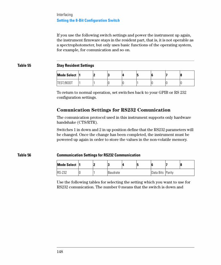
InterfacingSetting the 8-Bit Configuration Switch
If you use the following switch settings and power the instrument up again, the instrument firmware stays in the resident part, that is, it is not operable as a spectrophotometer, but only uses basic functions of the operating system, for example, for comunication and so on.
To return to normal operation, set switches back to your GPIB or RS 232 configuration settings.
Comunication Settings for RS232 Comunication
The comunication protocol used in this instrument supports only hardware handshake (CTS/RTR).
Switches 1 in down and 2 in up position define that the RS232 parameters will be changed. Once the change has been completed, the instrument must be powered up again in order to store the values in the non-volatile memory.
Use the following tables for selecting the setting which you want to use for RS232 comunication. The number 0 means that the switch is down and
Table 55 Stay Resident Settings
Mode Select 1 2 3 4 5 6 7 8
TEST/BOOT 1 1 0 0 1 0 0 0
Table 56 Communication Settings for RS232 Communication
Mode Select 1 2 3 4 5 6 7 8
RS-232 0 1 Baudrate Data Bits Parity
148

InterfacingSetting the 8-Bit Configuration Switch
1 means that the switch is up. Please note that there are two possible switch settings for 9600 baud
Table 57 Baudrate Settings
Switches Baud Rate Switches Baud Rate
3 4 5 3 4 5
0 0 0 9600 1 0 0 9600
0 0 1 1200 1 0 1 14400
0 1 0 2400 1 1 0 19200
0 1 1 4800 1 1 1 38400
Table 58 Data Bit Settings
Switch 6 Data Word Size
0 7 Bit Comunication
1 8 Bit Comunication
Table 59 Parity Settings
Switches Parity
7 8
0 0 No Parity
1 0 Odd Parity
1 1 Even Parity
149

InterfacingSetting the 8-Bit Configuration Switch
150
Warranty Statement
Warranty Statement
All Chemical Analysis Products
Agilent Technologies (Agilent) warrants its chemical analysis products against defects in materials and workmanship. For details of the warranty period in your country, call Agilent. During the warranty period, Agilent will, at its option, repair or replace products which prove to be defective. Products that are installed by Agilent are warranted from the installation date, all others from the ship date.
If buyer schedules or delays installation more than 30 days after delivery, then warranty period starts on 31st day from date of shipment (60 and 61 days, respectively for products shipped internationally).
Agilent warrants that its software and firmware designed by Agilent for use with a CPU will execute its programming instructions when properly installed on that CPU. Agilent does not warrant that the operation of the CPU, or software, or firmware will be uninterrupted or error-free.
Limitation of Warranty
Onsite warranty services are provided at the initial installation point. Installation and onsite warranty services are available only in Agilent service travel areas, and only in the country of initial purchase unless buyer pays Agilent international prices for the product and services. Warranties requiring return to Agilent are not limited to the country of purchase.
For installation and warranty services outside of Agilent’s service travel area, Agilent will provide a quotation for the applicable additional services.
If products eligible for installation and onsite warranty services are moved from the initial installation point, the warranty will remain in effect only if the customer purchases additional inspection or installation services, at the new site.
The foregoing warranty shall not apply to defects resulting from:
1 improper or inadequate maintenance, adjustment, calibration, or operation by buyer,
2 buyer-supplied software, hardware, interfacing or consumables,
3 unauthorized modification or misuse,
151

Warranty Statement
4 operation outside of the environmental and electrical specifications for the product,
5 improper site preparation and maintenance, or
6 customer induced contamination or leaks.
THE WARRANTY SET FORTH IS EXCLUSIVE AND NO OTHER WARRANTY, WHETHER WRITTEN OR ORAL, IS EXPRESSED OR IMPLIED. AGILENT SPECIFICALLY DISCLAIMS THE IMPLIED WARRANTIES OF MERCHANTABILITY AND FITNESS FOR A PARTICULAR PURPOSE.
Limitation of Remedies and Liability
THE REMEDIES PROVIDED HEREIN ARE BUYER’S SOLE AND EXCLUSIVE REMEDIES. IN NO EVENT SHALL AGILENT BE LIABLE FOR DIRECT, INDIRECT, SPECIAL, INCIDENTAL, OR CONSEQUENTIAL DAMAGES (INCLUDING LOSS OF PROFITS) WHETHER BASED ON CONTRACT, TORT OR ANY OTHER LEGAL THEORY.
Responsibilities of the Customer
The customer shall provide:
1 access to the products during the specified periods of coverage to perform maintenance,
2 adequate working space around the products for servicing by Agilent personnel,
3 access to and use of all information and facilities determined necessary by Agilent to service and/or maintain the products (insofar as these items may contain proprietary or classified information, the customer shall assume full responsiblity for safeguarding and protection from wrongful use),
4 routine operator maintenance and cleaning as specified in the Agilent operating and service manuals, and
5 consumables such as paper, disks, magnetic tapes, ribbons, inks, pens, gases, solvents, columns, syringes, lamps, septa, needles, filters, frits, fuses, seals, detector flow cell windows, and so on.
152

Warranty Statement
Responsibilities of Agilent Technologies
Agilent Technologies will provide warranty services as described in the following table.
Table 60 Warranty Services
Services During Warranty* Warranty Period** Type
Agilent CE instruments,Agilent 1100 Series LC modules,Agilent 8453 UV-visible spectrophotometers
1 Year Onsite
CE, LC, UV-visible supplies and accessories 90 Days Onsite
Columns and consumables*** 90 Days Return to Agilent
Gas discharge and tungsten lamps 30 Days Return to Agilent
Repairs performed onsite by Agilent**** 90 Days Onsite
* This warranty may be modified in accordance with the law of your country. Please consult your local Agilentoffice for the period of the warranty, for shipping instructions and for the applicable wording of the localwarranty.** Warranty services are included as specified for chemical-analysis products and options purchasedconcurrently provided customer is located within a Agilent-defined travel area. Agilent warranty serviceprovides for 8 a.m. to 5 p.m. onsite coverage Monday through Friday, exclusive of Agilent holidays.*** Columns and consumables are warranted to be free from defects for a period of 90 days after shipment andwill be replaced on a return-to-Agilent basis if unused.**** Agilent repair warranty is limited to only the item repaired or replaced.
153

Safety Information
Safety Information
The following general safety precautions must be observed during all phases of operation, service, and repair of this instrument. Failure to comply with these precautions or with specific warnings elsewhere in this manual violates safety standards of design, manufacture, and intended use of the instrument. Agilent Technologies assumes no liability for the customer’s failure to comply with these requirements.
General
This is a Safety Class I instrument (provided with terminal for protective earthing) and has been manufactured and tested according to international safety standards.
Operation
Before applying power, comply with the installation section. Additionally the following must be observed.
Do not remove instrument covers when operating. Before the instrument is switched on, all protective earth terminals, extension cords, auto-transformers, and devices connected to it must be connected to a protective earth via a ground socket. Any interruption of the protective earth grounding will cause a potential shock hazard that could result in serious personal injury. Whenever it is likely that the protection has been impaired, the instrument must be made inoperative and be secured against any intended operation.
Make sure that only fuses with the required rated current and of the specified type (normal blow, time delay, and so on) are used for replacement. The use of repaired fuses and the short-circuiting of fuseholders must be avoided.
Some adjustments described in the manual, are made with power supplied to the instrument, and protective covers removed. Energy available at many points may, if contacted, result in personal injury.
Any adjustment, maintenance, and repair of the opened instrument under voltage should be avoided as much as possible. When inevitable, this should be carried out by a skilled person who is aware of the hazard involved. Do not attempt internal service or adjustment unless another person, capable of
154

Safety Information
rendering first aid and resuscitation, is present. Do not replace components with power cable connected.
Do not operate the instrument in the presence of flammable gases or fumes. Operation of any electrical instrument in such an environment constitutes a definite safety hazard.
Do not install substitute parts or make any unauthorized modification to the instrument.
Capacitors inside the instrument may still be charged, even though the instrument has been disconnected from its source of supply. Dangerous voltages, capable of causing serious personal injury, are present in this instrument. Use extreme caution when handling, testing and adjusting.
Safety Symbols
WARNING A warning alerts you to situations that could cause physical injury or
damage to the equipment. Do not proceed beyond a warning until you
have fully understood and met the indicated conditions.
CA UTIO N A caution alerts you to situations that could cause a possible loss of data. Do not proceed beyond a caution until you have fully understood and met the indicated conditions.
Table 61 Safety Symbols used on Instruments and in Manuals
Symbol Description
The apparatus is marked with this symbol when the user should refer to the instruction manual in order to protect the apparatus against damage.
Indicates dangerous voltages.
Indicates a protected ground terminal.
Eye damage may result from directly viewing light produced by deuterium lamps used in detectors and spectrophotometers. Always turn off the deuterium lamp before opening the lamp door on the instrument.
!
155

Solvent Information
Solvent Information
Observe the following recommendations on the use of solvents.
Flow Cells
Avoid the use of alkaline solutions (pH > 9.5) which can attack quartz and thus impair the optical properties of flow cells.
Solvents
Always filter solvents, small particles can permanently block capillaries. Avoid the use of the following steel-corrosive solvents:
• Solutions of alkali halides and their respective acids (for example, lithium iodide, potassium chloride, and so on).
• High concentrations of inorganic acids like nitric acid, sulfuric acid especially at higher temperatures (replace, if your analysis method allows, by phosphoric acid or phosphate buffer which are less corrosive against stainless steel).
• Halogenated solvents or mixtures which form radicals and/or acids, for example:
2CHCl3 + O2 → 2COCl2 + 2HCl
This reaction, in which stainless steel probably acts as a catalyst, occurs quickly with dried chloroform if the drying process removes the stabilizing alcohol.
• Analysis-grade ethers, which can contain peroxides (for example, THF, dioxane, di-isopropylether) such ethers should be filtered through dry aluminium oxide which adsorbs the peroxides.
• Solutions of organic acids (acetic acid, formic acid, and so on) in organic solvents. For example, a 1-% solution of acetic acid in methanol will attack steel.
• Solutions containing strong complexing agents (for example, EDTA, ethylene diamine tetra-acetic acid).
• Mixtures of carbon tetrachloride with 2-propanol or THF.
156

Radio Interference
Radio Interference
Manufacturer’s Declaration
This is to certify that this equipment is in accordance with the Radio Interference Requirements of Directive FTZ 1046/1984. The German Bundespost was notified that this equipment was put into circulation, the right to check the series for compliance with the requirements was granted.
Test and Measurement
If test and measurement equipment is operated with equipment unscreened cables and/or used for measurements on open set-ups, the user has to assure that under operating conditions the radio interference limits are still met within the premises.
157

Sound Emission
Sound Emission
Manufacturer’s Declaration
This statement is provided to comply with the requirements of the German Sound Emission Directive of 18 January 1991.
This product has a sound pressure emission (at the operator position) < 70 dB.
• Sound Pressure Lp < 70 dB (A)
• At Operator Position
• Normal Operation
• According to ISO 7779:1988/EN 27779/1991 (Type Test)
158

Lithium Batteries Information
Lithium Batteries Information
WARNING Danger of explosion if battery is incorrectly replaced. Replace only
with the same or equivalent type recommended by the equipment
manufacturer.
Do not dispose of lithium batteries in domestic waste.
Transportation of discharged lithium batteries through carriers
regulated by IATA/ICAO, ADR, RID, IMDG is not allowed. Discharged
lithium batteries must be disposed of locally according to national
waste disposal regulations for batteries.
159

Agilent Technologies on Internet
Agilent Technologies on Internet
For the latest information on products and services visit our worldwide web site on the Internet at:
http://www.agilent.com/go/chem
160

Index
Numerics1 MByte memory, 11816-bit A/D converter, 314 Mbyte memory, 1188-bit configuration switch, 1468-channel peristaltic pump, 53
AA/D converter, 31absorbance
averaging, 46calculation, 35, 46, 47conversion of raw data to, 43run buffer, 46spectra, 46
accessing lamps, 25accessory boards
control, 43removing, 118, 120
accessory slot, 25accuracy
photometric, 12wavelength, 12
acquisition of spectra, 46additional memory, 118air (compressed), 104altitude, 11analog-to-digital converter, 31antistatic
bags, 108grounding kit, 108
APG remote connector, 56application-specific integrated circuit
(ASIC), 35ASIC, 35attaching
the light pipe to main power supply, 135
the power button, 134autosampler, 52
connector, 52averaging
of intensity spectra, 46of signal data, 35
Bbaseline flatness, 13battery for NVRAM, 35
baudratesettings, 149
binary code of GPIB address, 146blank push button, 23block diagram
of electronics, 29of main power supply, 32of SLS board, 39of SPM board, 34of SSI board, 42
boardsspectrograph connector interface
(SCI), 38spectrophotometer data acquisition
(SDA), 30spectrophotometer interface (SSI),
42spectrophotometer lamp supply
(SLS), 30spectrophotometer processor main
(SPM), 30spectrophotometer sipper interface
(SSI), 30, 31, 38, 109, 116burn hazard, 98
Ccabinet, 26cables, 51
general-purpose-GPIO, 54multichannel pump-GPIO, 53power supply, 63sipper/sampler-GPIO, 51sipper-GPIO, 51valve controller-GPIO, 54
calculationof absorbance, 35, 46, 47of variance, 36
CAN connector, 25, 58certification of computers, 10chassis of instrument, 122, 123cleaning
lenses, 94the Instrument, 95the instrument, 94the lenses, 103the source lens, 103the spectrograph lens, 105
clock, 35
collimated beam, 19compartment for sample, 20compensation for photodiode array
temperature, 35compressed air, 104computers, 10
connections to, 50comunication protocol, 148comunication settings for RS232 comu-
nication, 148connecting
plugs of lamps, 99connections
internal, 62to computer, 50to peripherals, 50
connectorAPG remote, 56autosampler, 52CAN, 25, 58definitions, 63fan, 63GPIB, 25GPIO, 24, 51, 52, 53main power supply, 63multicell transport, 24, 57pump, 51, 52, 53remote, 24RS232, 24RS232C, 58shutter assembly, 64tungsten lamp, 65valve, 54
construction and layout of instrument, 26
controlof interfaces, 43of MIO and accessory boards, 43
conversionof raw data to absorbance, 43to absorbance spectra with variance,
43converter, A/D, 31correction
factors for temperature, 45for dark current, 35, 45for gain, 45for offset, 35
161

Index
for stray light, 19, 20, 35, 46, 47for temperature, 45
covers, 109removing, 109, 113replacing, 111, 114
CTS/RTR hardware handshake, 148
Ddamage to eyes, 97dark current correction, 35, 45dark-corrected intensity spectra, 45data bit settings, 149description
of firmware, 43of instrument, 22
detergent, 95deuterium lamp, 19, 47, 64, 96
connecting plugs, 99connector, 64current control, 40exchanging, 94, 96filament control, 40fixing, 99ignition, 40light emission, 40removing, 96replacing, 99
deuterium line data, 47diagnostic
A/D converter, 40functions, 43
dimensions, 11diode array, 21disconnecting the lamp cables, 97door to access lamps, 25
EEEPROM, 38eight-bit configuration switch, 146eight-channel peristaltic pump, 53electromagnetic interference, 26electronically-programmable logic de-
vice (EPLD), 38electronics overview, 29electrostatic discharge, 108emission
of deuterium lamp, 40of radio frequencies, 26
162
emission linesof deuterium lamp, 47of mercury lamp, 47of zinc-argon lamp, 47
E-Pak packaging, 26EPLD (electronically-programmable
logic device), 38European Pharmacopoeia, 13exchanging
internal memory, 118key pad, 116keyboard, 116the deuterium lamp, 94, 96the fan assembly, 126the main power supply, 133the optical unit, 122the SDA board, 128the shutter assembly, 124the SLS board, 130the SPM board, 120the tungsten lamp, 94, 96
exploded views, 138external
cabinet, 26cables, 51communication, 50
eye damage, 97
Ffan assembly, 126
exchanging, 126removing, 126replacing, 126
fan cable, 120, 121, 126fan connector, 63filament control of deuterium lamp, 40filter for stray-light correction, 19, 20,
47fingerprints on lamp, 98firmware
description, 43loading errors, 147resident part of, 43update procedures, 147updates, 43
fixing lamps, 99flatness of baseline, 13flow of raw data, 43
forced cold start settings, 147front covers
parts, 142removing, 109replacing, 111
front panel, 42front view of spectrophotometer, 22fuse, 32
Ggain
correction, 45table, 45
general-purpose-GPIO cable, 54GPIB
address, 146connector, 25
GPIO connector, 24, 51, 52, 53grating, 19, 21grounding kit, 108
Hhardware fuse, 32hardware handshake (CTS/RTR), 148hazard
eye damage, 97skin burn, 98
holographic grating, 19, 21humidity, 11
Iignition of deuterium lamp, 40indicator, 22industrial design of spectrophotome-
ter, 26input load, 50instrument
description, 22layout and construction, 26parts breakdown, 139, 141
integration time, 46intensity
averaging, 46run buffer, 47test, 96
interface control, 43interference, 26internal

Index
cabinet, 26connections, 62events, 43
internal memoryexchanging, 118upgrading, 118
isopropanol, 102, 103isopropyl alcohol, 102, 103
Kkey pad, 116
exchanging, 116removing, 116replacing, 116
keyboard, 112, 116exchanging, 116removing, 116replacing, 116
keyboard cableremoving, 109
kinetics measurements, 118
Llamps, 19
access through door, 25deuterium, 19, 40, 47, 96do not ignite, 96fixing, 99lifetime, 98mercury, 47tungsten, 19, 40, 96zinc-argon, 47
layout and construction of instrument, 26
lens, 19, 21lenses
cleaning, 103photographic, 102, 104
lifetime of lamp, 98light emission of deuterium lamp, 40light pipe, 133, 134
removing, 134line centroids, 48line frequency, 11line power
input socket, 25switch, 22
line voltage, 11
lock mechanism, 96logarithm of intensity spectrum, 46logic true, 50low-pass filter, 38, 42LPS board, 120, 121
Mmain microprocessor, 35main power supply, 32
block diagram, 32connector, 63exchanging, 133removing, 133replacing, 134reset, 33
maintenance, 94procedures, 94
materials, 138measure push buttons, 23memory, 36
exchanging, 118non-volatile random access, 35program, 35system, 35upgrading, 118
mercury lamp, 47metal
front cover, 111internal cabinet, 26lamp door, 96, 99
microprocessor, 35system, 43
MIO boardcontrol, 43removing, 118, 120slot, 25
mode select, 146multicell transport
connector, 24, 57multichannel pump-GPIO cable, 53
NNIST 2034 standard, 12, 14NIST 930e standard, 12, 14noise, 13nominal spectral slit width, 21non-volatile random access memory
(NVRAM), 35, 146
NVRAM, 35
Ooffset correction, 35open collector type, 50operating
altitude, 11temperature, 11
optical system, 19optical tissue, 98optical unit, 122
exchanging, 122removing, 122replacing, 123
overload, 32overtemperature sensor, 33overview
of electronics, 29of optical system, 19
Pparity settings, 149parts, 138
breakdown, 139, 141front cover, 142list, 138numbers, 138
PDA (photodiode array), 38front end processor (PFP), 38signal conditioning electronics, 38
performance specifications, 12peripherals
connections to, 50peristaltic pump, 51personal computers, 10photodiode array, 21, 30, 38, 45
quantum efficiency, 45temperature compensation, 35
photographic lenses, 102, 104cleaning brush, 102, 104, 105
photometricaccuracy, 12noise, 13stability, 13
physical specifications, 11plasma discharge, 19plastic
door, 25
163

Index
external cabinet, 26front cover, 109, 112lamp door, 96, 99
potassium dichromate, 12power button, 134power consumption, 11power supply cable, 63program memory, 35pulse width modulation driver (PWM),
35pump connector, 51, 52, 53push buttons, 23
blank, 23sample, 23standar, 23stop, 23
Qquantum efficiency of the photodiode
array, 45quartz envelope, 98
Rradiated frequency interference (RFI),
38radiation source, 19radio frequency emissions, 26random access memory, non-volatile,
35range of wavelengths, 12raw data, 45
conversion to absorbance, 43flow from photodiode array, 43
real-pass band function, 48real-time clock, 35rear cover
removing, 113replacing, 114
rear view of spectrophptometer, 24recalibration, 48remote connector, 24removing
accessory boards, 118, 120connectors and screws from SPM
board, 121covers, 109key pad, 116keyboard, 116
164
MIO board, 118, 120SIMM memory modules, 118the deuterium lamp, 96the fan assembly, 126the front covers, 109the keyboard cable, 109the light pipe, 134the main power supply, 133the middle rear foam block, 130the optical unit, 122the rear cover, 113the sample pan, 110, 113the SDA board, 128the shutter assembly, 101, 124the SLS board, 130the SPM board, 120the tungsten lamp, 96
repair procedures, 108repairing the instrument, 108replacing, 109
covers, 109key pad, 116keyboard, 116SIMM memory modules, 119the deuterium lamp, 99the fan assembly, 126the front covers, 111the main power supply, 134the middle rear foam block, 131the optical unit, 123the rear cover, 114the sample pan, 111, 114the SDA board, 129the shutter assembly, 102, 125the SLS board, 131the SPM board, 121the tungsten lamp, 99the upper rear foam block, 121
reproducibility, 12reset of power supply, 33resident
EEPROM, 38part of firmware, 43, 148
resolution, 12RFI (radiated frequency interference),
38ribbon cables on SDA and LPS boards,
120, 121
RS232Cconnector, 24, 58settings, 148
Ssafety
light switches, 41shutdown, 41
samplecompartment, 20, 110, 111, 113, 114pan, 110, 111, 113, 114push button, 23
sampling interval, 21scan time, 13SCI board, 38SDA board, 30, 120, 121
exchanging, 128removing, 128replacing, 129
security lever, 25sensor for overtemperature, 33setting the 8-bit configuration switch,
146sheet-metal
door, 25rear cover, 114
shine-through aperture, 19shortest scan time, 13shutdown, 41shutter, 19, 20shutter assembly
connector, 64exchanging, 124removing, 101, 124replacing, 102, 125
shutter cable, 101, 102, 120, 121, 124, 125
signalaveraging, 35conditioning electronics, 45level, 50
SIMMmemory module, 36memory modules, 118, 119socket, 118sockets, 30
single-channel peristaltic pump, 51sipper/sampler-GPIO cable, 51

Index
sipper-GPIO cable, 51slit, 19, 21slit width, 12, 21slots for MIO and accessory boards, 25SLS board, 30
exchanging, 130removing, 130replacing, 131
source lens, 19, 20cleaning, 103surface, 102, 103
source of radiation, 19specifications
performance, 12physical, 11
spectra and signal processor (SSP), 35spectral
acquisition, 46averaging, 46
spectrograph, 20, 30connector interface board (SCI), 38lens, 19, 21lens, cleaning, 105slit, 19
spectrophotometerdata acquisition board (SDA), 30front view, 22industrial design, 26interface board (SSI), 42lamp supply board (SLS), 30processor main board (SPM), 30rear view, 24sipper interface board (SSI), 30, 31,
38, 109, 116SPM board, 30
block diagram, 34exchanging, 120removing, 120removing connectors and screws,
121replacing, 121
SSI board, 30, 31, 38, 42, 109, 116block diagram, 42
stability, 13standard push button, 23standard TTL levels, 50standards, 14
for photometric accuracy, 14
for wavelength accuracy, 14NIST 2034, 12, 14NIST 930e, 12, 14potassium dichromate, 12
status indicator, 22stay resident settings, 147stop push button, 23stray light, 12, 22stray-light correction, 19, 20, 30, 35, 46,
47filter, 47
subtract dark current, 45surface of source lens, 102, 103system memory, 35
Ttemperature
compensation of photodiode, 35correction, 45effects, 45filter, 45operating, 11sensor, 33
TEST/BOOT mode select, 146time
for shortest scan, 13for typical scan, 13until next scan, 13
tungsten lamp, 19, 96connecting plugs, 99connector, 65exchanging, 94, 96fixing, 99removing, 96replacing, 99voltage control, 40
typical scan time, 13
Uupgrading
internal memory, 118
Vvalve connector, 54valve controller-GPIO cable, 54variance, 43
calculation, 36
Wwavelength
accuracy, 12axis linearization, 47calibration table, 47range, 12reproducibility, 12
weight, 11width of slit, 12, 21wired-or technique, 50wrist strap, 108
Zzinc-argon lamp, 47
165

Index
166

saIn This Book
This handbook is intended for the technical reader who needs background information about the Agilent 8453 spectrophotometer and potential repairs.
The handbook contains specifications of the spectrophotometer as well as descriptions of front and back panels, for example, where to connect accessories. Electronics are explained at block-diagram level. There is a detailed section about troubleshooting to help find a defective subassembly, such as an electronic board, in case the spectrophotometer does not operate any more. Part replacement procedures as well as an exploded view with part numbers are given for ordering and replacing assemblies.
For information about installation of the system including the spectrophotometer, computer and accessories, see the Installing Your
UV-Visible Spectroscopy System handbook.

Agilent Technologies
Agilent ChemStation
Understanding Your ChemStationUnderstanding Your Agilent ChemStation

Understanding Your Agilent ChemStation
Notices© Agilent Technologies, Inc. 2004, 2005-2009
No part of this manual may be reproduced in any form or by any means (including elec-tronic storage and retrieval or translation into a foreign language) without prior agree-ment and written consent from Agilent Technologies, Inc. as governed by United States and international copyright laws.
Manual Part NumberG2070-91126
Edition07/09
Printed in Germany
Agilent TechnologiesHewlett-Packard-Strasse 8 76337 Waldbronn
Warranty
The material contained in this docu-ment is provided “as is,” and is sub-ject to being changed, without notice, in future editions. Further, to the max-imum extent permitted by applicable law, Agilent disclaims all warranties, either express or implied, with regard to this manual and any information contained herein, including but not limited to the implied warranties of merchantability and fitness for a par-ticular purpose. Agilent shall not be liable for errors or for incidental or consequential damages in connection with the furnishing, use, or perfor-mance of this document or of any information contained herein. Should Agilent and the user have a separate written agreement with warranty terms covering the material in this document that conflict with these terms, the warranty terms in the sep-arate agreement shall control.
Technology Licenses The hardware and/or software described in this document are furnished under a license and may be used or copied only in accor-dance with the terms of such license.
Restricted Rights LegendIf software is for use in the performance of a U.S. Government prime contract or subcon-tract, Software is delivered and licensed as “Commercial computer software” as defined in DFAR 252.227-7014 (June 1995), or as a “commercial item” as defined in FAR 2.101(a) or as “Restricted computer soft-ware” as defined in FAR 52.227-19 (June 1987) or any equivalent agency regulation or contract clause. Use, duplication or dis-closure of Software is subject to Agilent Technologies’ standard commercial license terms, and non-DOD Departments and Agencies of the U.S. Government will
receive no greater than Restricted Rights as defined in FAR 52.227-19(c)(1-2) (June 1987). U.S. Government users will receive no greater than Limited Rights as defined in FAR 52.227-14 (June 1987) or DFAR 252.227-7015 (b)(2) (November 1995), as applicable in any technical data.
Safety Notices
CAUTION
A CAUTION notice denotes a hazard. It calls attention to an operating procedure, practice, or the like that, if not correctly per-formed or adhered to, could result in damage to the product or loss of important data. Do not proceed beyond a CAUTION notice until the indicated condi-tions are fully understood and met.
WARNING
A WARNING notice denotes a hazard. It calls attention to an operating procedure, practice, or the like that, if not correctly performed or adhered to, could result in personal injury or death. Do not proceed beyond a WARNING notice until the indi-cated conditions are fully under-stood and met.
For Research Use Only
Software RevisionThis guide is valid for B.04.xx revisions of the Agilent ChemStation software, where xx refers to minor revisions of the software that do not affect the technical accuracy of this guide.

Understanding Your Agilent ChemStation 3
In This Guide...
In This Guide...
This guide describes various concepts of the Agilent ChemStation. It is intended to increase your understanding of how the ChemStation works.
For information on using the ChemStation please refer to the general help system and the Online help "Tutorial".
1 Agilent ChemStation Features
This chapter summarizes main components and features of the Agilent ChemStation.
2 Methods
This chapter describes the concepts of methods and how to work with them.
3 Data Acquisition
This chapter describes the concepts of Data Acquisition, data files, logbook, and more.
4 Integration
This chapter describes the concepts of integration the ChemStation integrator algorithms. It describes the integration algorithm, integration and manual integration.
5 Quantification
This chapter describes how ChemStation does quantification. It gives details on area% and height% calculations, external standard (ESTD) calculation, norm% calculation, internal standard (ISTD) calculation, and quantification of unidentified peaks.
6 Peak Identification
This chapter describes the concepts of peak identification.

4 Understanding Your Agilent ChemStation
In This Guide...
7 Calibration
This chapter describes Calibration in the ChemStation.
8 Automation
This chapter describes the concepts of automation. It explains how to work with sequences in ChemStation, what happens when a sequence is run and how to customize sequences.
9 Data Review, Reprocessing and Batch Review
This chapter describes the possibilities to review data and how to reprocess sequence data. In addition it describes the concepts of Batch Review, Batch configuration, review functions, and batch reporting.
10 Using the ChemStation Reports
This chapter describes what a report is. It gives details on reporting results, quantitative results, report styles, report destination, and sequence summary reporting.
11 Evaluating System Suitability
This chapter describes what the ChemStation can do to evaluate the performance of both the analytical instrument before it is used for sample analysis and the analytical method before it is used routinely and to check the performance of analysis systems before, and during, routine analysis.
12 System Verification
This chapter describes the verification function and the GLP verification features of the ChemStation.

Understanding Your Agilent ChemStation 5
Contents
Contents
1 Agilent ChemStation Features 9
General Description 11ChemStation Hardware 14About the ChemStation Software 15Instrument Control 31Documentation 32The ChemStation Directory Structure 34Navigation Pane 38
2 Methods 41
What is a Method? 42Parts of a Method 43Status of Methods 46Creating Methods 48Editing Methods 49Method Directory Structure 51What Happens When a Method is Run? 52Method Operation Summary 57
3 Data Acquisition 59
What is Data Acquisition? 60Data Files 61Online Monitors 63Logbook 64Status Information 65
4 Integration 67
What is Integration? 69What Does Integration Do? 70The ChemStation Integrator Algorithms 71Overview 73Definition of Terms 77

6 Understanding Your Agilent ChemStation
Contents
Principle of Operation 79Peak Recognition 80Baseline Allocation 89Peak Area Measurement 102Integration Events 105Manual Integration 110
5 Quantification 113
What is Quantification? 114Quantification Calculations 115Correction Factors 116Uncalibrated Calculation Procedures 118Calibrated Calculation Procedures 119ESTD Calculation 120Norm% Calculation 122ISTD Calculation 123
6 Peak Identification 127
What is Peak Identification? 128Peak Matching Rules 129Types of Peak Identification 130Absolute Retention/Migration Time 132Corrected Retention/Migration Times 134Peak Qualifiers 136The Identification Process 139
7 Calibration 141
Definition of Terms 142Calibration Table 143Calibration Curve 144Unknown Samples 146Types of Calibration 147Group Calibration 153Peak Summing 154Recalibration 155

Understanding Your Agilent ChemStation 7
Contents
8 Automation 159
What is Automation? 161What is a Sequence/Sequence Template? 162Preferences - Sequence Tab 163Sequence Parameters 165Sequence Table 166Creating Sequences (Sequences and Sequence Templates) 167Working with Sequences (Sequences and Sequence Templates) 169Sequence Log File 172What Happens When a Sequence is Run? 173Sequence Data File Structure (Unique Folder Creation ON) 175Data File Naming in a Sequence 176Postsequence Operation 178Automatic Recalibration 179Specifying Recalibrations 180Types of Sequences 183Explicit Calibration Sequences 184Cyclic Single-Level Calibration Sequences 185Cyclic Multiple-Level Calibration Sequences 186Explicit and Cyclic Calibrations Together 190Cyclic Calibration Sequences with Bracketing 192Cyclic Recalibration Sequences with Multiple Vials Containing the Same Dilution of a Standard 196
9 Data Review, Reprocessing and Batch Review 201
Navigation Table in Data Analysis 202What is Batch Review? 207Enabling Batch Review Functionality with ChemStation OpenLAB Option Installed 208Batch Configuration 209Review Functions 211Batch Reporting 212
10 Using the ChemStation Reports 213
What is a Report? 214Reporting Results 215Quantitative Results 217

8 Understanding Your Agilent ChemStation
Contents
Reporting Custom Field Values 219Report Styles 220Other Report Style Parameters 223Report Destination 224Sequence Summary Reporting 226
11 Evaluating System Suitability 231
Noise Determination 235Calculation of Peak Symmetry 240System Suitability Formulae and Calculations 242General Definitions 243Performance Test Definitions 244Definitions for Reproducibility 250Internally Stored Double Precision Number Access 255
12 System Verification 259
Verification and Diagnosis Views 260The GLPsave Register 263DAD Test Function 265

9
Understanding Your Agilent ChemStation
Agilent Technologies
1Agilent ChemStation Features
General Description 11
Additional Instrument Modules 12
Additional Data Evaluation Modules 12
Data Evaluation-only Products 13
ChemStation Hardware 14
About the ChemStation Software 15
Operating System 15
Methods and Sequences 15
System Configuration 15
Data Model 16
File Naming Conventions 16
Software User Interface 18
Data Acquisition 19
Data Analysis — Display 20
Data Analysis — Integration 21
Data Analysis — Quantification 22
Data Analysis — Data Review, Data Reprocess and Batch Review 22
Data Analysis — Standard Reporting 23
Data Analysis — Specialized Reporting 23
Utilities and Compatibilities 26
Customization 26
Automation 27
Good Laboratory Practice 28
Instrument Control 31
Networking 31
Documentation 32
The ChemStation Directory Structure 34
Navigation Pane 38

10 Understanding Your Agilent ChemStation
1 Agilent ChemStation FeaturesIn This Guide...
Navigation Buttons 38
ChemStation Explorer 38
This chapter summarizes main components and features of the Agilent ChemStation.

Understanding Your Agilent ChemStation 11
Agilent ChemStation Features 1General Description
General Description
The ChemStations for GC, LC, LC/MSD, CE, CE/MSD, and A/D systems are instrument control, data acquisition and data evaluation systems for
• Agilent 7890A Gas Chromatographs,
• Agilent 6890N, 6890Plus and 6890A Gas Chromatographs,
• Agilent 6850 Gas Chromatographs,
• 5890 Series II Gas Chromatograph
• Agilent 1100/1200 Series modules and systems for LC,
• Agilent 1100 Series LC/MSD,
Agilent 6100 Series Single Quad LC/MSD
• Agilent 1600 Capillary Electrophoresis (CE) system,
• Agilent 7100 Capillary Electrophoresis (CE) system,
• Agilent CE/MS system, and
• Agilent 35900E dual channel analog-to-digital interface.
The software is designed to run on IBM-compatible personal computers under Microsoft® Windows XP Professional operating environment.
The software is sold as a single instrument basic ChemStation in five versions. All versions include data acquisition, instrument control, data analysis (integration, quantification and reporting), automation and customization for one analytical instrument. An instrument is defined as running on a single timebase, but can collect data from a number of different detectors simultaneously. The five versions are:
• a single instrument ChemStation for gas chromatography (GC) systems, product number G2070BA,
• a single instrument ChemStation for liquid chromatography (LC) systems, product number G2170BA,
• a single instrument ChemStation for capillary electrophoresis (CE) systems, product number G1601BA,
• a single instrument ChemStation for liquid chromatography/mass selective detector (LC/MSD) systems, product number G2710BA, and

12 Understanding Your Agilent ChemStation
1 Agilent ChemStation FeaturesGeneral Description
• a single instrument analog-to-digital (A/D) ChemStation for analog data acquisition with external event control, product number G2072BA.
The instrument control capability of the ChemStation software may be expanded by purchasing additional instrument data acquisition and control modules to allow multiple instrument, mixed technique configurations.
Additional Instrument Modules
The additional instrument modules are:
• additional GC instrument control and data acquisition module, product number G2071BA,
• additional LC instrument control and data acquisition module, product number G2171BA,
• additional CE instrument control and data acquisition module, product number G2172BA,
• LC/MSD instrument control, data acquisition, and data evaluation add-on module, product number G2712BA
• additional analog data acquisition module, product number G2073BA, and
• MSD Add-on Module to upgrade an LC system to LC7MSD, product number G2712BA.
Additional Data Evaluation Modules
The data processing capability of the ChemStations may also be expanded through the purchase of additional data processing modules for specialist applications:
• additional diode array detector (DAD) spectral evaluation module, product number G2180BA,
• additional ChemStore sample organization and results database module, product number G2181BA, and
• LC/MSD deconvolution and bioanalysis data evaluation module, product number G2720BA, for use with the LC/MSD ChemStation only.
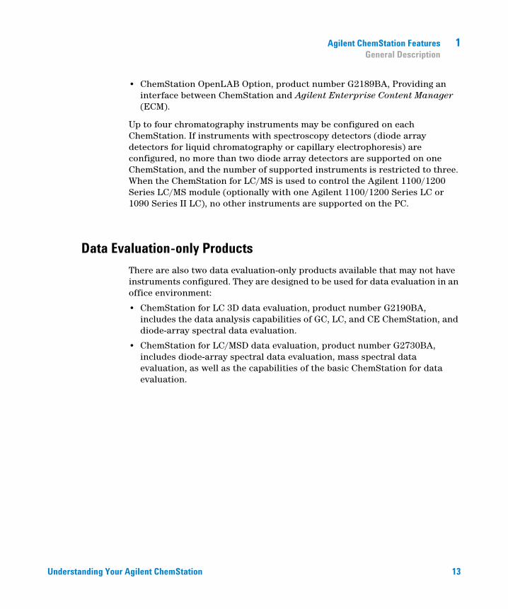
Understanding Your Agilent ChemStation 13
Agilent ChemStation Features 1General Description
• ChemStation OpenLAB Option, product number G2189BA, Providing an interface between ChemStation and Agilent Enterprise Content Manager (ECM).
Up to four chromatography instruments may be configured on each ChemStation. If instruments with spectroscopy detectors (diode array detectors for liquid chromatography or capillary electrophoresis) are configured, no more than two diode array detectors are supported on one ChemStation, and the number of supported instruments is restricted to three. When the ChemStation for LC/MS is used to control the Agilent 1100/1200 Series LC/MS module (optionally with one Agilent 1100/1200 Series LC or 1090 Series II LC), no other instruments are supported on the PC.
Data Evaluation-only Products
There are also two data evaluation-only products available that may not have instruments configured. They are designed to be used for data evaluation in an office environment:
• ChemStation for LC 3D data evaluation, product number G2190BA, includes the data analysis capabilities of GC, LC, and CE ChemStation, and diode-array spectral data evaluation.
• ChemStation for LC/MSD data evaluation, product number G2730BA, includes diode-array spectral data evaluation, mass spectral data evaluation, as well as the capabilities of the basic ChemStation for data evaluation.

14 Understanding Your Agilent ChemStation
1 Agilent ChemStation FeaturesChemStation Hardware
ChemStation Hardware
For details of ChemStation hardware, see the Agilent ChemStation Installation Manual for your respective system.

Understanding Your Agilent ChemStation 15
Agilent ChemStation Features 1About the ChemStation Software
About the ChemStation Software
Operating System
The ChemStation requires Microsoft Windows XP Professional SP3 or Windows Vista Business SP1 operating system.
The ChemStation Control Charts feature requires MicroSoft Excel.
Methods and Sequences
The analytical method fully describes how a particular separation is performed. It contains all parameters for instrument control, data acquisition and evaluation, including integration, quantification and reporting. The system may be set up to acquire data from a number of samples by different methods. The control file for this sort of operation is called a sequence, and holds the individual sample information, references to the appropriate methods, and automatic recalibration specifications. For further information on methods and sequences, see “Automation” on page 27 and the online help system.
System Configuration
The configuration of the instrument system is done through the configuration editor program. It allows you to define your instruments, their GPIB or LAN addresses, the directories for your data, sequences and methods and the color definition for the ChemStation software. For further information, see the handbooks supplied with the additional ChemStation modules.

16 Understanding Your Agilent ChemStation
1 Agilent ChemStation FeaturesAbout the ChemStation Software
Data Model
The ChemStation software is designed around a data model based on a memory structure called a register. Registers are multipurpose structures that can hold analytical data and information for both two-dimensional information (for example, time/intensity) and three-dimensional information (for example, time/intensity/wavelength).
The ChemStation provides commands and functions to construct, expand, extract and, where it does not alter primary data, edit registers. For further information, see the Macro Programming Guide which is available as online help.
File Naming Conventions
Naming Conventions
The following rules enable the ChemStation to create and process valid names for files and directories:
The following characters are not allowed as part of a file or directory name:
• < > : " / \ | @ % * ? ' & blanks (spaces) etc.
Using these characters in file or directory names may cause problems when loading files in ChemStation. In addition, if these characters are used in the installation folder, the reprocessing copy does not start, if the character % is used in the installation folder, some 'Agilent Chemstation B.04.02' shortcuts do not work properly.
The following rules apply in addition:
Table 1 Restricted characters
ChemStation parameter Character
Method File Names: % and . (decimal point) are not allowed
Data File Names (Prefix/Counter): blanks are not allowed
Data Subdirectory and Sequence Subdirectory: [] + = ; , . (decimal point); spaces are not allowed

Understanding Your Agilent ChemStation 17
Agilent ChemStation Features 1About the ChemStation Software
The following reserved device names cannot be used as the name of a file:
• CON, PRN, AUX, NUL
• COMx (where x is a number from 1 to 9)
• LPT1x (where x is a number from 1 to 9)
Also avoid these names followed by an extension (e.g. Nul.txt).
Maximum Length of ChemStation file names and subdirectories
The Agilent ChemStation specifications for file names and subdirectories are listed below:
NOTE English, Japanese, and Chinese operating systems are used to test naming conventions. Agilent cannot give a support statement for non-English operating systems and their special characters.
Table 2 Maximum Length of ChemStation file names and subdirectories
DataFile/Subdirectory/Path Max. Input Length
Auto append
Example
Data file name 38 .D Demodad.d
Data file name using prefix/counter 15 .D longname000001.d
Method Sequence Hypersequence Libraries Customized Report Templates
40 . M. S. HYP. UVL. FRP
def_lc.m def_lc.s def_lc.hyp demodad.uvl areapct.frp
Data file subdirectory 40 demo (in sample info)
Data sequence subdirectory 40 demo (in sequence parameters)

18 Understanding Your Agilent ChemStation
1 Agilent ChemStation FeaturesAbout the ChemStation Software
All ChemStation logbooks report system messages in an extended format and information strings are printed over multiple lines. Certain reports, e.g. Sequence report, may truncate filenames to fit all information onto the report template.
Software User Interface
The ChemStation user interface is designed into Views that group software functionality according to typical analytical tasks. The following three standard views are present in all software configurations:
• the Method and Run Control view for controlling and acquiring data from the instrument,
• the Data Analysis view for reviewing and reevaluating data that has been acquired,
• the Report Layout view for designing specific report layouts, and
Additional views are present if additional data evaluation modules have been ordered or for certain instrument configurations that support instrument diagnostics and verification procedures. A ChemStation Companion view is available for when it is desirable to have instrument operators run samples from an easy-to-use, preconfigured table.
Sequence Data Container Name 40 test_date_time (create using sequence preferences)
Data Path Method Path Sequence PathHypersequence Path Libraries PathCustomized Report Template Path
100 100 c:\chem32\1\datac:\chem32\1\methods c:\chem32\1\sequence c:\chem32\1\hyper c:\chem32\speclib c:\chem32\repstyle
Table 2 Maximum Length of ChemStation file names and subdirectories
DataFile/Subdirectory/Path Max. Input Length
Auto append
Example

Understanding Your Agilent ChemStation 19
Agilent ChemStation Features 1About the ChemStation Software
The Navigation Pane contains the Navigation Button, to allow rapid switching between the ChemStation views, and the tree-based ChemStation Explorer. The contents of the ChemStation Explorer are view-dependent, giving access to different ChemStation elements.
Each view consists of a set of standard user elements including menus and toolbars. The standard toolbar provides rapid access to the common system specification information such as methods and sequences. The Method and Run Control view additionally incorporates a system status bar, a sample information area, that may be configured for single runs or automated runs, and a schematic instrument interface diagram for GC, CE and LC configurations. The schematic instrument interface diagram uses hot spots to allow rapid access to instrument parameters and an animated graphical overview of the status of each analysis as it proceeds. The schematic instrument diagram may be turned off if it is not required, to save memory and other Windows resources.
The Data Analysis view extends the standard toolbar to specific data analysis modes including integration, calibration, reporting, annotation, signal comparison and additional specialized modes if the modules are installed. Each of these separate data analysis modes are supported with a mode-specific toolset.
The Report Designer view allows the user to graphically define the layout of a specific report style in a graphical object orientated fashion. It also uses a set of toolbars specific to this task.
Data Acquisition
The status of the instrument is continually monitored and updated on the display, along with the elapsed run time of the analysis both when the software is a visible window and when it is iconized. The transactions that occur during the analysis, including any errors and the instrument conditions at the start and the end of the analysis, are recorded in the system’s logbook, an extract of which is stored with every data file.
The instrument conditions, such as flow, temperature, pressure and solvent composition for liquid chromatographs may be recorded and stored with each data file. These instrument parameters can be displayed and plotted to testify

20 Understanding Your Agilent ChemStation
1 Agilent ChemStation FeaturesAbout the ChemStation Software
to the quality of each analysis. The exact nature of the parameters recorded depends both on the technique and the capabilities of the configured instrument.
One or more display windows may be used to monitor the data being acquired by the instrument in real time. The data are displayed in real measurement units such as mAU, Volts, degrees or bar. The windows may each show multiple overlaid chromatographic/electropherographic signals or instrument parameters, such as pressure. The display default settings may be adjusted and are remembered by the system so users can set their own preferred settings as the instrument default. The window has zoom capability and the cursor may be used to display a specific signal’s response at any point in time.
During an analysis, the complete functionality of the ChemStation can be used through the offline copy. While acquisition is running, the Data Analysis part of the online session of an instrument is not accessible, and data review has to be performed in the offline copy.
A snapshot function is available for users who wish to start processing data before the analysis is completed. The snapshot has to be taken in the offline copy of the instrument sessions and is immediately present for review.
The layout of the signal and status information windows, including the components of the schematic instrument interface diagram is saved automatically.
For further information on Data Acquisition, see “Data Acquisition” on page 59 and the online help system.
Data Analysis — Display
The Data Analysis view extends the standard tool bar with task-grouped data analysis functions including integration, calibration, reporting, annotation, and signal comparison toolsets. The following key graphical operations are possible:
• single or multisignal displays selectable when loading the chromatogram/electropherogram,
• overlays of chromatogram/electropherogram from different samples,
• subtraction of one chromatogram/electropherogram from another,

Understanding Your Agilent ChemStation 21
Agilent ChemStation Features 1About the ChemStation Software
• graphical vertical and horizontal alignment of signals to help visual comparison,
• signal inversion or mirroring to help visual comparison,
• graphical zoom and scrolling functions,
• adjustment of display attributes including selection of tick marks, baselines, axes, retention/migration times and compound names (the user can also select the font for the RT and compound labels, adjust the size and orientation of the display, select the display as overlaid or separated and select scaling factors),
• the chromatogram/electropherogram display may include graphical overlays of instrument parameters depending on the capability of the configured instrument,
• user-defined annotations may be interactively added to the display, with the selection of font, size, text rotation and color (once defined, the annotations may be graphically moved, edited or deleted),
• copy the display to the Windows clipboard in both metafile and bitmap format,
• a pick mode function to display the values of individual data points in detector units, and
• export of time/intensity digitized points to the Microsoft Windows clipboard.
Data Analysis — Integration
The ChemStation integrator algorithm is the second revision of a new generation aimed at improved ruggedness, reliability and ease-of-use.

22 Understanding Your Agilent ChemStation
1 Agilent ChemStation FeaturesAbout the ChemStation Software
Data Analysis — Quantification
The ChemStation’s calibration mode of the data analysis view allows simultaneous display of:
• the signal or signals being calibrated with an indication of the current compound’s retention/migration time window,
• the calibration table whose display may be configured from a comprehensive selection of calibration parameters, and
• the calibration curve for the compound being calibrated.
All the calibration mode windows are linked so that changes in one are automatically reflected in all the others. This mode allows graphical selection and modifications of the calibration data.
Quantification is based on %, Normalized %, External standard, External standard %, Internal standard and Internal standard % calculations calculated on either peak area or height. Calibrations may be multilevel and include multiple internal standard definitions. Calibration histories are automatically saved and can be used to weight the recalibration calculations.
For information on calibration and quantitation, see “Calibration” on page 141.
Data Analysis — Data Review, Data Reprocess and Batch Review
The following two additional toolsets are available within the Data Analysis view :
• Navigation Table
• Batch Review
The Navigation Table makes possible several key graphical operations:
• standard table configuration features, such as sorting, drag-and-drop options, column selection, item grouping to specify a preferred navigation table configuration
• right mouse click functions to load a signal, overlay a signal, export data, print reports
• review signal details by expanding a line in the navigation table

Understanding Your Agilent ChemStation 23
Agilent ChemStation Features 1About the ChemStation Software
• review signals and create ChemStation reports using either loaded methods or the individual data file method DA.M, for example, to review manual integration events
• reprocess sequence data (acquired sequence data from ChemStation Rev. B.02.01 and later)
The following key graphical operations are possible in the Batch Review:
• define automatic or manual review and reprocess of (calibrated) data files
• recalibration of calibration table
• review compound tables of calibrated methods
• create specific batch reports
Data Analysis — Standard Reporting
A standard set of user-definable report styles for sample reporting can be selected from the report specification screen. Every standard report type contains standard information groups and optional information groups.
For more information on the report styles available, see “Using the ChemStation Reports” on page 213.
Data Analysis — Specialized Reporting
Advanced reporting capabilities are also included in the ChemStation for applications that require a more specialized set of reports. These include statistics on separation quality, reports that include trend analysis between samples and user-defined report layouts.
System Suitability Reports
System suitability reports enable users to report system performance parameters for individual analyses. There are three variations, or styles of these reports.
The standard template Performance report prints parameters for uncalibrated methods that include:
• retention/migration time,

24 Understanding Your Agilent ChemStation
1 Agilent ChemStation FeaturesAbout the ChemStation Software
• capacity factor (k’),
• peak area,
• peak height,
• symmetry,
• true peak width at half height,
• efficiency in plate numbers,
• resolution, and
• selectivity.
For calibrated methods the compound name and amount replace the peak area, height and selectivity columns.
The report header includes the standard header and footer, sample information block, the analytical column parameters and optionally a plot of the chromatogram/electropherogram.
The Performance and Noise style adds an evaluation of the signal noise, in up to seven user-defined evaluation ranges, to the data from the Performance report style. The noise parameters are reported as signal to noise ratios for each peak or calibrated compound and a noise table for each signal. Each noise table includes noise calculated by the six times standard deviation, peak to peak and ASTM methods as well as the wander and drift.
The Extended Performance style adds plots of each individual peak graphically showing the peak start and stop times, half width and baseline. This style includes the following parameters in addition to the ones reported by the standard Performance reports:
• area, height and amount,
• skew,
• excess,
• usp tailing factor,
• time interval between data points and number of data points over the peak,
• statistical moments (M0 to M4),
• peak width at half height calculated by the true, five sigma, tangent and tailing methods, and
• plate/column and plates/meter calculated by the peak width at half height, five sigma, tangent and statistical methods.

Understanding Your Agilent ChemStation 25
Agilent ChemStation Features 1About the ChemStation Software
Users may define their own noise evaluation ranges and acceptable limits for these performance criteria. Values lying outside the user-defined acceptable limits are indicated on the report.
For more information on system suitability calculations, see “Evaluating System Suitability” on page 231.
Sequence Summary Reports
Sequence summary reports are produced at the end of a series of automated analyses. Their range of application is from a brief summary of the samples analyzed to a detailed graphical repeatability or trend analysis of user-selectable parameters between different samples, analyzed by the same method.
For more information on sequence summary reporting, see the online help system and “Sequence Summary Reporting” on page 226.
Customized Reports
A customized reporting design view is included in the ChemStation for users who want to define the exact content of their own reports. The user graphically defines a report layout which may include general sample information, signal, integration and quantitative analytical result information. The user may define individual elements, such as text, tables and graphics, organize them in information sections and graphically adjust their relative position size and orientation of each defined element. The individual sections may be added, deleted, reordered and nested.
The user may define headers and footers to appear on every page, time stamps for the report and page numbering in the page x of y format. The information included in the report may be any ChemStation or user-defined parameter.
Once the report has been designed it may be associated with a particular method to make it the default report format for that particular type of analysis.
Customized reports may be output to the screen, printer and to a file. Reports to the screen include graphics.
For more information on the report layout, see the online help system.

26 Understanding Your Agilent ChemStation
1 Agilent ChemStation FeaturesAbout the ChemStation Software
Control Chart Reports
A Control Chart feature is included with the ChemStation software. Once this feature is installed and selected, the user may automatically track a selected parameter of a compound each time a method is run. These parameters include: Amount, Response Factor, retention/migration Time, and Area.
For more information on these Custom and Control Chart reports, see the online help system.
Utilities and Compatibilities
The ChemStation can import and export data files in the andi (Analytical Data Interchange) chromatography format of the Analytical Instrument Association (AIA), revision 1.0, copyright 1992. Data import is supported at compliance level one (sample information and signal data) and data export at compliance level two (sample information, signal data and integration results).
The ChemStation includes commands and functions to support the dynamic data exchange (DDE) standard of the Microsoft Windows platform as both a DDE client and a DDE server. The command set includes commands to establish and terminate connections, transfer information in both directions and execute remote functions.
Customization
The ChemStation can be customized using the powerful command set. These commands may be grouped to execute automatically a specific function; such a group is called a macro. Users writing macros may define their own variables, build in conditional or looping constructs, perform physical I/O including file handling and user interaction, nest their macros and schedule and exchange data with other MS-DOS or Microsoft Windows applications.
For more information on customization, see the Macro Programming Guide which is available as online help.

Understanding Your Agilent ChemStation 27
Agilent ChemStation Features 1About the ChemStation Software
Automation
The ChemStation can execute multimethod sequences.
The sequence parameter set may be defined to use automatically generated files or sequentially numbered files with a user-defined prefix of up to fifteen characters. The user may select to run full analyses or data reprocessing only sequences and can also select one of a series of technique specific shutdown commands or a user-defined shutdown macro that runs when the sequence terminates either by error or after all the analyses are completed.
The sequence table, or list of analyses to run, is built in a spreadsheet-like user interface that allows users to specify vial numbers and sample names, analysis methods, sample quantification parameters including sample amount, a multiplier and dilution factor, calibration specification, data exchange parameter LIMSID and the number of repeat injections. Depending of the configured instruments and modules, more fields will accessible, e.g. if an Agilent 1100/1200 LC system includes a fraction collector, the “Fract. Start” column will appear in the sequence table. The appearance of the sequence table can be configured by the user. The user can jump between individual cells in the table and copy, cut or paste individual cells or entire rows or series of rows in order to build sequences efficiently and quickly.
Samples may be identified in the sequence table as unknowns, calibration or control sample types. The sample type determines any special data evaluation treatment of the sample:
• unknown samples are evaluated and reported according to the method specification,
• calibration samples are used to recalibrate the quantification component of the method as described below, and
• control samples are evaluated against the limits for each component defined in the method. If the results lie outside any specified parameter range the execution of the sequence will be halted.
Calibration samples may be defined as simple, cyclic or bracketed. Simple recalibrations mean a recalibration occurs each time a calibration sample is defined in the sequence. Cyclic recalibrations occur at defined intervals during analysis of a series of unknowns. In bracketing a series of unknown samples, two calibration sets are analyzed. The quantitative reports for the unknown samples are then calculated using a calibration table averaged between the two calibration sets.

28 Understanding Your Agilent ChemStation
1 Agilent ChemStation FeaturesAbout the ChemStation Software
The partial sequence functionality allows users to see the order of execution of the sequence and also select individual sample entries to rerun or re-evaluate. When re-evaluating data already acquired users can specify whether reprocessing uses the original sample quantification data or new data entered in the sequence’s sample table.
Sequences may be paused to run single injection priority samples by another method, then restarted without disrupting the automation. Samples can be added to the sequence table while the sequence is executing.
Both the sequence and partial sequence tables may be printed.
For more information on sequences, see “Automation” on page 159, and the online help system.
Good Laboratory Practice
The ChemStation is developed to internationally recognized design and development standards and has a number of features specifically to help users operating in a regulated environment. These features are in the area of complete method specification and verification that the methods are fit for their intended use, to check the operation of their system and ensure the traceability, originality and quality of the data.
Development Process
The Certificate of Validation shipped with each software package documents the software development and testing steps executed as part of the development cycle. The development process is registered to the ISO 9001 quality standard. It is documented together with onsite revalidation protocols in the Validation BinderAgilent ChemStation for LC.
Method Specification and Use
• Global methods — the complete instrument and data analysis specification is stored in one place. Methods include individual compound range specifications to check that quantification results are not applied outside the calibrated range.

Understanding Your Agilent ChemStation 29
Agilent ChemStation Features 1About the ChemStation Software
• The method change history log allows users of a validated method to automatically record how and when a method was changed. Users may optionally add a comment reason to the change history log. The change history log is automatically stored as part of the method in a binary format. To prevent unauthorized access to the records, it is protected by the user access scheme, described below. The change history log may be viewed and printed.
• Limits may be assigned on a compound-by-compound basis in each method for a number of chromatographic/electropherographic and system performance parameters, as described in the data analysis quantification section. Results exceeding these parameter ranges are used to control the execution of automated sequences as described in the automation section. They are indicated on the appropriate analysis report.
• System performance or suitability reports (see the Reporting section above) provide detailed analysis of the separation quality.
The ChemStation may be configured for restricted access for two user access levels, an operator and manager level. The manager level may be password protected and allows access to the complete ChemStation functionality. The operator level restricts the user to key functionality and executing defined analytical methods. The operator level is intended for use in routine laboratories and specifically prevents users from modifying and creating new methods.
Method Robustness
Sequence summary reports (see “Sequence Summary Reporting” on page 226) provide a means to test methods for robustness. The extended format reports for user selected criteria, are reported as trend charts and may be used to determine the realistic operation limits. These limits can then be incorporated in the method to ensure, through the analysis of control samples, that the method is operating within specifications.
System Operation
The ChemStation verification kit, which is part of the standard software, automatically checks for the correct installation and operation of the data evaluation parts of the software by comparing results generated when the test is executed against prerecorded known values. The verification kit allows users to define their own data files and methods to be the basis of the test.

30 Understanding Your Agilent ChemStation
1 Agilent ChemStation FeaturesAbout the ChemStation Software
Data Traceability, Originality and Quality
Run-time logbook provides a transaction log of the complete system. It also records any unusual events (such as errors or parameter changes made during a run) as well as the instrument conditions before and after each analysis. A copy of the relevant logbook extract is saved with each data file.
The actual instrument conditions, such as pressure, flow, and temperature, that occurred during each analysis are also recorded if the configured instrument supports this capability. This data can be subsequently displayed graphically with the chromatogram/electropherogram to show the actual instrument conditions during that particular analysis, as well as being included on the report.
Methods saved with the data file record the actual method at the time of the analysis and allows the complete reconstruction of the reported data at a later date. The method is saved at the completion of all the analytical steps.
All reports have time stamps and traceable page numbering (page x of y pagination style). The user may select the level of detail in each report ranging from simple summary reports to complete system details (see the Reporting section above).
GLP Save register files, specified as part of the method configuration, save all the original data, including sample information, data analysis method, chromatographic/electropherographic signals, instrument conditions, integration and quantification results, report data and the run logbook in one checksum protected binary file. This is an uneditable binary format that ensures the originality of the results.The file includes a revisioning scheme that indicates if data has been reprocessed.
Control sample types may be defined in the sequence table and used to automatically check the instrument performance against quality control sample results when the instrument is running unattended. Results that are outside the user-specified acceptable range will stop the automatic execution of the instrument.

Understanding Your Agilent ChemStation 31
Agilent ChemStation Features 1Instrument Control
Instrument Control
The instrument control capability of the ChemStation may be expanded through the purchase of additional instrument modules to allow multiple instrument, mixed technique configurations. For further information, see the handbook(s) supplied with the additional ChemStation modules.
Networking
The ChemStation is tested and supported with Agilent’s LanManager software, Microsoft Windows XP Professional and Microsoft Windows Vista Business products based on the IEEE 802.3 CSMA/CD specification. It should be compatible with any networking software compatible with the programming standards of Microsoft Windows.
These products enable the ChemStation to share physical devices such as plotters and printers with other laboratory computers as well as sharing information such as data files and methods.
Client/Server
The ChemStation software may be installed on a suitable network server and downloaded onto the client PCs as required. Each client specific configuration ensures a suitable environment for different techniques and individual users while the centralized software installation relieves the burden of managing many copies of the same ChemStation installation in one work environment.
LAN-based instrument control
The ChemStation software provides LAN-based instrument control and data acquisition for the Agilent 7890 GC, the Agilent 6890 GC, the Agilent 35900E A/D control module and the Agilent 1100/1200 Series LC. You can easily control and monitor instruments by connecting them to a LAN on which the ChemStation PC resides. This arrangement allows the ChemStation PC to be located remotely from the instruments it controls.

32 Understanding Your Agilent ChemStation
1 Agilent ChemStation FeaturesDocumentation
Documentation
The documentation set contains specific sections on:
• Installing and learning the ChemStation software,
• Using the ChemStation software,
• Understanding the principles of how the software works, and
• Customizing the ChemStation.
Installing and Learning
Each ChemStation software product comes with an installation manual that includes details of the key steps in PC hardware and software requirements, instrument interface installation, ChemStation installation and installation qualification. The installation manual is specific to the purchased configuration and may include troubleshooting, system records and system maintenance advice.
Using the Software
Two additional categories of online information are designed for the routine user.
The ChemStation includes comprehensive, Windows-style, context-sensitive and indexed online help. This system gives detailed explanations of every screen and the meaning of the parameters on that screen. The detailed explanations are backed up by graphics where appropriate, and may be copied to the Windows clipboard for incorporation into the users’ own documentation, or for printing.
An Online Tutorial included in the online help enables you to learn the software while working on your own methods and data. It provides an overview of the first steps in data acquisition and data analysis.
The How To part of the online help also includes check lists of the more complex technique-specific and common chromatography tasks to help less frequent users who want to be sure they set up the system correctly. These checklists are linked directly to the detailed online help information.

Understanding Your Agilent ChemStation 33
Agilent ChemStation Features 1Documentation
Understanding the Principles
The Understanding Your ChemStation manual documents the principles of the software operation and the algorithms used in the data manipulations.
Customization
Sophisticated users who wish to customize the operation of the ChemStation, or who want to build in additional features, may do so by writing macros.
The primary reference manual, Macro Programming Guide which is available as online help, has a comprehensive set of functional examples backed up by a complete description of the internal data types and structures.
The commands help file, accessed directly from the ChemStation’s Help menu or the Show Command dialog box, is the programmer’s function reference. It includes syntax and parameter explanations with example macros illustrating the use of many of the commands. By virtue of being online, the users can copy the examples and command syntax directly into their own macro source files.

34 Understanding Your Agilent ChemStation
1 Agilent ChemStation FeaturesThe ChemStation Directory Structure
The ChemStation Directory Structure
The following example shows the directory structure of the ChemStation. It comprises generic directories that are shared by all configured instruments and instrument-specific directories. The software installation program creates a subdirectory of the ChemStation directory (by default CHEM32) for each configured instrument with the instrument number. Inside this subdirectory, the data, methods and sequences for this instrument are stored by default. Additional subdirectories for data, methods and sequences can be added using Preferences. Within the ChemStation Explorer, is it then possible to navigate to the newly added locations in order to load data, methods and sequences. The new locations are also available in each selection box within the ChemStation menu items (for example, for the path settings in the Sequence Parameters).
The ChemStation subdirectories are as follows:

Understanding Your Agilent ChemStation 35
Agilent ChemStation Features 1The ChemStation Directory Structure
Figure 1 ChemStation Directory Structure

36 Understanding Your Agilent ChemStation
1 Agilent ChemStation FeaturesThe ChemStation Directory Structure
Table 3 ChemStation subdirectories
Directory Contents
Chem32 The directory comprises the programs to configure and start the ChemStation software. It must be part of the PATH variable. This directory is added automatically by the installation program unless you provide an alternative.
REPSTYLE Used for report templates defined using the Report Template Editor.
CORE Used for the core components of the software shared by all chromatographic/electropherographic instrument configurations. This is the working directory of the ChemStation.
PICTURES Comprises graphics needed by the ChemStation.
Language Used for the language-specific code of this part of the software.
1024, 800, ToolbarSupport Files
Comprise initialization files for the graphical user interface. Do not change.
helpenu Used for the US-English version of the help files for the appropriate software part.
BACKUP Used for backup copies of old files during installation.
DRIVERS Comprises instrument drivers.
1 Used for the configured instrument (1 to 4). This subdirectory comprises five additional subdirectories: DATA, METHODS, SEQUENCE, VERIFY, and TEMP.
DATA Comprises the default result directories of your analyses. It can also comprise more subdirectories if you structure the disk with subdirectories as you work, by defining them using the Sample Information or Sequence Parameters dialog box. Result directories are identified by a name with a .D extension. For more information on the structure of data files, see “Data Acquisition” on page 59. Additional data paths can be added using Preferences.
METHODS Comprises the default master method directories that have a .M extension. For further details on the contents, see “Method Directory Structure” on page 51. Additional method paths can be added using Preferences.

Understanding Your Agilent ChemStation 37
Agilent ChemStation Features 1The ChemStation Directory Structure
SEQUENCE Comprises the default path for sequence templates. The sequence templates in these directories have a .S extension. Additional sequence paths can be added using Preferences, see “Preferences - Sequence Tab” on page 163 and “Sequence Parameters” on page 165.
VERIFY Comprises data files, methods, and the results of data processing stored in register (.REG) files. These files execute the ChemStation verification procedure described in the online help. One set of data, method, and register files is used for each verification test.
TEMP The TEMP subdirectory comprises temporary work files and the logbook files. For example, for Instrument 1 the online logbook is called INSTR1.LOG and the offline logbook is called INSTR1-2.LOG.
LC, GC, CE, MS Instrument driver-specific code such as INI files.
IQT Comprises files the files needed for IQT report creation.
speclibs Comprises spectral libraries.
Table 3 ChemStation subdirectories
Directory Contents
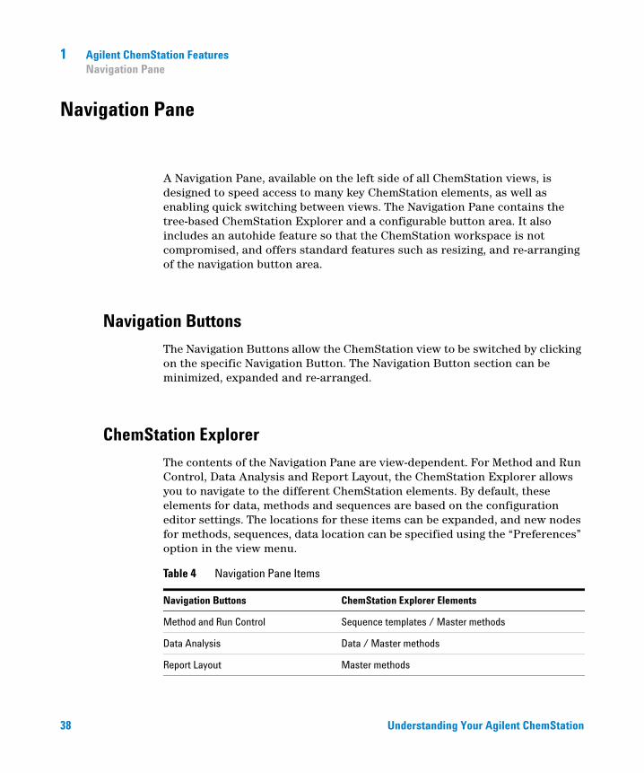
38 Understanding Your Agilent ChemStation
1 Agilent ChemStation FeaturesNavigation Pane
Navigation Pane
A Navigation Pane, available on the left side of all ChemStation views, is designed to speed access to many key ChemStation elements, as well as enabling quick switching between views. The Navigation Pane contains the tree-based ChemStation Explorer and a configurable button area. It also includes an autohide feature so that the ChemStation workspace is not compromised, and offers standard features such as resizing, and re-arranging of the navigation button area.
Navigation Buttons
The Navigation Buttons allow the ChemStation view to be switched by clicking on the specific Navigation Button. The Navigation Button section can be minimized, expanded and re-arranged.
ChemStation Explorer
The contents of the Navigation Pane are view-dependent. For Method and Run Control, Data Analysis and Report Layout, the ChemStation Explorer allows you to navigate to the different ChemStation elements. By default, these elements for data, methods and sequences are based on the configuration editor settings. The locations for these items can be expanded, and new nodes for methods, sequences, data location can be specified using the “Preferences” option in the view menu.
Table 4 Navigation Pane Items
Navigation Buttons ChemStation Explorer Elements
Method and Run Control Sequence templates / Master methods
Data Analysis Data / Master methods
Report Layout Master methods

Understanding Your Agilent ChemStation 39
Agilent ChemStation Features 1Navigation Pane
Verification (LC and LC/MS) Verification view-specific shortcuts
Diagnosis (LC and LC/MS) Diagnosis view-specific shortcuts
Tune (LC/MS) Tune view-specific shortcuts
Table 4 Navigation Pane Items
Navigation Buttons ChemStation Explorer Elements

40 Understanding Your Agilent ChemStation
1 Agilent ChemStation FeaturesNavigation Pane

41
Understanding Your Agilent ChemStation
Agilent Technologies
2Methods
What is a Method? 42
Parts of a Method 43
Method Information 43
Instrument Control 43
Data Analysis 44
Run-Time Checklist 45
Status of Methods 46
Stored Methods 46
Current Method 47
Creating Methods 48
Editing Methods 49
Method Parts to Edit 49
Method Directory Structure 51
What Happens When a Method is Run? 52
Method Operation 52
Pre-run Command or Macro (Run Time Checklist) 53
Data Acquisition (Run Time Checklist) 53
Data Analysis (Run Time Checklist) 54
Customized Data Analysis (Run Time Checklist) 55
Save GLP Data (Run Time Checklist) 55
Postrun Command or Macro (Run Time Checklist) 56
Save Copy of Method with Data (Run Time Checklist) 56
Save Copy of Method as DA.M with Data (ChemStation Default) 56
Method Operation Summary 57
This chapter describes the concepts of methods and how to work with them.

42 Understanding Your Agilent ChemStation
2 MethodsWhat is a Method?
What is a Method?
A method comprises all the parameters for acquisition and data analysis together with pre- and post-run tasks for a given sample, if they are needed.
The available methods (*.m) files are visible in the ChemStation Explorer. For quick and easy navigation, you can add additional method locations to the ChemStation Explorer selection tree using the Paths tab of the Preferences dialog box.
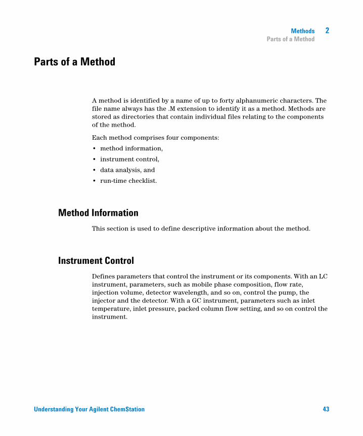
Understanding Your Agilent ChemStation 43
Methods 2Parts of a Method
Parts of a Method
A method is identified by a name of up to forty alphanumeric characters. The file name always has the .M extension to identify it as a method. Methods are stored as directories that contain individual files relating to the components of the method.
Each method comprises four components:
• method information,
• instrument control,
• data analysis, and
• run-time checklist.
Method Information
This section is used to define descriptive information about the method.
Instrument Control
Defines parameters that control the instrument or its components. With an LC instrument, parameters, such as mobile phase composition, flow rate, injection volume, detector wavelength, and so on, control the pump, the injector and the detector. With a GC instrument, parameters such as inlet temperature, inlet pressure, packed column flow setting, and so on control the instrument.

44 Understanding Your Agilent ChemStation
2 MethodsParts of a Method
Data Analysis
Defines parameters that control the data processing.
Signal Details
Defines signals and their properties used for data evaluation.
Integration Events
Defines timed events that will occur at specific retention/migration times on a chromatogram/electropherogram. These timed events can be used to change the way the signal is integrated.
Peak Identification
Defines data processing parameters associated with the identification of peaks in the chromatogram/electropherogram.
Peak Quantification
Defines data processing parameters that affect the quantification calculations which determine the amount or concentration of sample component corresponding to each peak.
Calibration and Recalibration
Defines data processing parameters that affect the calibration and how often calibration is done.
Custom Fields
Defines the properties of sample or compound related custom fields that are available for the method. The custom fields allow to add custom information to a sample or a compound in a sample.
Report
Defines the format of the report that is printed after a run.

Understanding Your Agilent ChemStation 45
Methods 2Parts of a Method
Run-Time Checklist
Defines which parts of the method are executed when the method is run.
You can use the run-time checklist to:
• acquire, store and process data to produce a report,
• execute only a portion of the method,
• acquire and store data without analyzing it,
• reanalyze existing data files,
• use your own macros for data analysis, pre- and post-run processing, and
• save the analysis results in a register for GLP purposes.

46 Understanding Your Agilent ChemStation
2 MethodsStatus of Methods
Status of Methods
A method can exist in two states: as a stored method, or as the current loaded method.
Stored Methods
These are methods stored on the computer disk. Stored methods have a name with up to forty alphanumeric characters followed by the extension .M. Methods are stored in the ChemStation in up to three locations:
• The Master Method is stored in a methods subdirectory, available in a Methods node of the ChemStation Explorer, and is not directly associated with any data container.
• When a sequence is run (using the option Unique Folder Creation ON (see “Preferences - Sequence Tab” on page 163), copies of all the master methods used in the sequence are stored in the sequence data container along with the sequence data files. These methods are directly linked to the sequence, and are used as well when the sequence is reprocessed. Changes to these methods are not propagated to the master methods. Changes are propagated to the Sequence Container Method as well to the individual methods (DA.M) during the sequence is reprocessed. If you now want to use the updated sequence container method for data acquisition, you need either to
• copy this method from the sequence data container to one of the defined method paths or
• use the save as option to save the updated method as a master method.
The new/updated method is then available in the ChemStation Explorer in the method view as a master method.
• In addition, two copies of the method used to run a sample are stored with the data files - the data file individual methods ACQ.M and DA.M. ACQ.M is the acquisition method, DA.M is the data analysis method. DA.M is the method that is loaded along with the data file if the Load DA method from data file checkbox in the Signal Options tab of the Preferences dialog box is
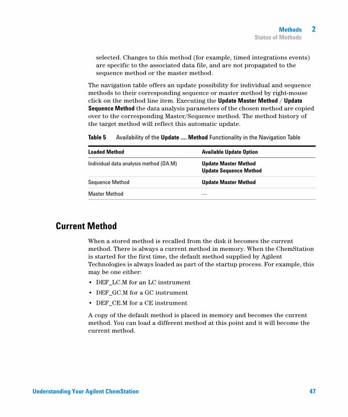
Understanding Your Agilent ChemStation 47
Methods 2Status of Methods
selected. Changes to this method (for example, timed integrations events) are specific to the associated data file, and are not propagated to the sequence method or the master method.
The navigation table offers an update possibility for individual and sequence methods to their corresponding sequence or master method by right-mouse click on the method line item. Executing the Update Master Method / Update Sequence Method the data analysis parameters of the chosen method are copied over to the corresponding Master/Sequence method. The method history of the target method will reflect this automatic update.
Current Method
When a stored method is recalled from the disk it becomes the current method. There is always a current method in memory. When the ChemStation is started for the first time, the default method supplied by Agilent Technologies is always loaded as part of the startup process. For example, this may be one either:
• DEF_LC.M for an LC instrument
• DEF_GC.M for a GC instrument
• DEF_CE.M for a CE instrument
A copy of the default method is placed in memory and becomes the current method. You can load a different method at this point and it will become the current method.
Table 5 Availability of the Update .... Method Functionality in the Navigation Table
Loaded Method Available Update Option
Individual data analysis method (DA.M) Update Master MethodUpdate Sequence Method
Sequence Method Update Master Method
Master Method ---

48 Understanding Your Agilent ChemStation
2 MethodsCreating Methods
Creating Methods
Creating a new method always means modifying the current method and saving the modifications under a new method name. Be aware that when the current method is changed, the disk version remains unchanged until you save your changes.
You have a choice of how to create a method. You can create a method to do either one or all parts of an analysis. For example, you can create a method to do only data acquisition. When you are ready to analyze the data and generate a library search report, you can then modify the method to do these data processing tasks.
NOTE When you load a method to run a sample, always load a master method from a method node in the ChemStation Explorer. You should avoid using sequence methods (from a sequence data container) or individual methods associated with data files (ACQ.M or DA.M).
NOTE Do not delete the default method (DEF_LC.M, DEF_CE.M or DEF_GC.M). These method files are used as templates to create new methods.

Understanding Your Agilent ChemStation 49
Methods 2Editing Methods
Editing Methods
You can edit an existing method using the Edit Entire Method item of the Method menu. You are guided through all the method dialog boxes and at the end you can save the method. This process is shown below:
Figure 2 Editing Method
Method Parts to Edit
Each method comprises four components that can be edited separately.
Some of the following subsections refer to specific dialog boxes, and some are generalized descriptions.
• Method Information comprises:
• a text description about the method.

50 Understanding Your Agilent ChemStation
2 MethodsEditing Methods
• Instrument Control depends on the configuration, and can comprise, for example:
• oven parameters,
• injector parameters, and
• detector parameters.
• Data Analysis comprises:
• signal details,
• integration parameters,
• quantification parameters,
• calibration parameters,
• custom field setup parameters, and
• reporting parameters.
• Run Time Checklist comprises:
• the parts of the method that will be executed.
NOTE Remember that methods can be stored in three locations in the ChemStation. Be sure that you are editing the correct method.

Understanding Your Agilent ChemStation 51
Methods 2Method Directory Structure
Method Directory Structure
A method comprises a group of files stored in the method directory.
The methods subdirectory comprises all the method subdirectories that have a .M extension. Additional methods subdirectories can be added using the preference settings.
Method files with the .MTH extension contain parameter sets and are in UNICODE format. The file INFO.MTH comprises the method control parameters.
Method files containing the instrument parameters have the name of the related analytical module. For example:
Table 6 Method file examples
HPCE1.MTH Comprises the acquisition method for the Capillary Electrophoresis.
ADC1.MTH Comprises the Agilent 35900 acquisition method. If two identical instruments are configured, the method files are called ADC1.MTH, ADC2.MTH.
DAMETHOD.REG For data evaluation.
LALS1.REG Comprises parameters for the Agilent 1100/1200 Series autosampler when a classic modular LC system is configured. The method files for the other Agilent 1100/1200 Series modules follow the same convention Lxxx1.reg where xxx is the module acronym.
AgilentSamplerDriver1.RapidControl.xxx.xml
Comprises parameters for the Agilent 1100/1200 Series autosampler when a modular LC system is configured. Several .xml files are present for the various parts of the parameters (indicated by the xxxpart of the file name). Similar .xml files are available for the other modules.

52 Understanding Your Agilent ChemStation
2 MethodsWhat Happens When a Method is Run?
What Happens When a Method is Run?
The run-time checklist dialog box specifies the parts of the method to execute when a run is started.
There are eight parts to the run-time checklist:
• pre-run command or macro,
• data acquisition,
• standard data analysis,
• analysis method for second signal (GC only),
• customized data analysis,
• save GLP data,
• post-run command or macro, and
• save copy of method with data (RUN.M).
When running a method the specified parts of the method defined in the Run Time Checklist dialog box are executed.
Method Operation
The figure shows an overview of the ChemStation status during the method operation, where all parts of the Run Time Checklist are selected.
NOTE Please note, that in case of the mode “Unique Folder Creation OFF" no ACQ.M and DA.M are generated. For more details please refer to “Preferences - Sequence Tab” on page 163.

Understanding Your Agilent ChemStation 53
Methods 2What Happens When a Method is Run?
Figure 3 Method Operation
Pre-run Command or Macro (Run Time Checklist)
If a pre-run command or macro is specified, it is executed before the analysis is started. This part is typically used for system customizing in conjunction with other software packages.
Data Acquisition (Run Time Checklist)
• All parameters are set to the initial conditions specified in the current method.
• If specified the injection program is executed and an injection is made from the currently defined vial.
• The monitor display shows the progress of the analysis including chromatographic/electropherographic information, and spectral data if available.
• Data are acquired and stored in a data file.

54 Understanding Your Agilent ChemStation
2 MethodsWhat Happens When a Method is Run?
• When the Data Acquisition is finished, copy of the currently executed method is stored as ACQ.M for the data file by default.
Data Analysis (Run Time Checklist)
When the stop-time has elapsed, the analysis is finished and all raw data is stored on the computer’s hard disk. The data analysis part of the software starts when all the raw data is stored.
Integration
• chromatogram/electropherogram objects in the signal are integrated as specified in the Integration Events dialog box.
• The start of the peak, the peak apex, retention/migration time and the end of the peak are determined.
• Baselines are defined under each peak to determine final peak height and area.
• The integration results are created as an Integration Results list.
Peak Identification and Quantification
• Using retention/migration times and optional peak qualifiers, the software identifies the peaks by cross-referencing them with known components defined in the calibration table.
• By using peak heights or peak areas the software calculates the amount of each detected component using the calibration parameters specified in the Calibration Table.
Spectra Library Search (ChemStations for LC 3D, CE, CE/MS and LC/MS Systems Only)
For all peaks that have UV-Visible spectra available, an automated search of a predefined spectral library may be done to identify the components in the sample based on the UV-Visible spectra. See Understanding Your Spectral Module for details.
Understanding Your Agilent ChemStation 55
Methods 2What Happens When a Method is Run?
Peak Purity Checking (ChemStations for LC 3D, CE, CE/MS and LC/MS Systems Only)
For a peak with UV-Visible spectra, you can calculate a purity factor for that peak and store it in a register. Peak purity may be determined automatically at the end of each analysis as part of the method, if the Check Purity box is checked when specifying an automated library search or when selecting an appropriate report style. See Understanding Your Spectral Module for details.
Print Report
A report is generated with identities and amounts of components detected in the run.
Customized Data Analysis (Run Time Checklist)
Enables you to run your own customized macros to evaluate your analytical data.
Save GLP Data (Run Time Checklist)
Saves the binary register GLPSave.Reg together with the data analysis method in the default data file subdirectory. This feature is designed to help prove the originality of the data and the quality of the individual analysis.
The GLPSave.Reg binary file contains the following information in a non-editable, checksum-protected, register file:
• key instrument set points (can be graphically reviewed),
• chromatographic or electropherographic signals,
• integration results,
• quantification results,
• data analysis method, and
• logbook.

56 Understanding Your Agilent ChemStation
2 MethodsWhat Happens When a Method is Run?
These data are saved only if the Save GLP Data feature is activated by checking the check box in the runtime checklist. You can review, but not edit, GLP data in the data analysis menu of the ChemStation.
Postrun Command or Macro (Run Time Checklist)
If a postrun command or macro is specified it is executed after the data evaluation, for example, copying data to a disk for data backup.
Save Copy of Method with Data (Run Time Checklist)
This is done after data acquisition, and only if Data Acquisition is activated in the Run Time Checklist. It copies the current method to the data directory, named as RUN.M
Save Copy of Method as DA.M with Data (ChemStation Default)
Depending on the marked items in the Run Time Checklist, a copy of the current executed method is saved as DA.M along with the data file. This is done the execution of the last marked item in the Run Time Checklist, in general after the Standard Data Analysis part.

Understanding Your Agilent ChemStation 57
Methods 2Method Operation Summary
Method Operation Summary
The following list shows the flow of the method operation when all parts of the Run Time Checklist are selected.
1 Prerun Command Macro
Does a task before the analysis is started.
2 Data Acquisition
Does injector program.
Injects sample.
Acquires raw data.
Stores data.
3 Save Copy of Method with Data (RUN.M) - optional by Run Time Checklist
4 Save Copy of Method with Data (ACQ.M) - ChemStation default
5 Data Analysis (Process Data)
Loads data file.
Integrates data file.
Identifies and quantifies peak.
Searches spectral library if available.
Checks peak purity if available.
Prints report.
6 Customized Data Analysis
Executes your macros.
7 Save GLP Data
Saves binary register GLPSave.Reg
8 Postrun Command Macro
Does a task after completion of the analysis, for example, generates a customized report.
9 Save Copy of Method with Data (DA.M) - ChemStation default

58 Understanding Your Agilent ChemStation
2 MethodsMethod Operation Summary

59
Understanding Your Agilent ChemStation
Agilent Technologies
3Data Acquisition
What is Data Acquisition? 60
Data Files 61
Online Monitors 63
Online Signal Monitor 63
Online Spectra Monitor 63
Logbook 64
Status Information 65
ChemStation Status 65
Status Bar 65
System Diagram 66
This chapter describes the concepts of Data Acquisition, data files, logbook, and more.
60 Understanding Your Agilent ChemStation
3 Data AcquisitionWhat is Data Acquisition?
What is Data Acquisition?
During data acquisition, all signals acquired by the analytical instrument are converted from analog signals to digital signals in the detector. The digital signal is transmitted to the ChemStation electronically and stored in the signal data file.
The available data (*.d) files are visible in the ChemStation Explorer. For quick and easy navigation, you can add additional data file locations to the ChemStation Explorer selection tree using the Paths tab of the Preferences dialog box.

Understanding Your Agilent ChemStation 61
Data Acquisition 3Data Files
Data Files
A data file comprises a group of files, by default stored in the DATA directory as a subdirectory with a data file name and a .D extension. A data file name is can be defined manually using 40 characters including the extension. Each file in the directory follows a naming convention. Additional data directories can be added using the Preferences settings.
Table 7 Data files
Name Description
*.CH Chromatographic/electropherographic signal data files. The file name comprises the module or detector type, module number and signal or channel identification. For example, ADC1A.CH, where ADC is the module type, 1 is the module number and A is the signal identifier and .CH is the chromatographic extension.
*.UV UV spectral data files. The file name comprises the detector type and device number (only with diode array and fluorescence detector).
REPORT.TXT, REPORT.PDF
Report data files for the equivalent signal data files.
SAMPLE.MAC Sample information macro.
SAMPLE.MAC.BAC Backup of the original sample information macro. This file is created when the original sample parameters (like multipliers) are updated during reprocessing.
RUN.LOG Logbook entries which have been generated during a run. The logbook keeps a record of the analysis. All error messages and important status changes of the ChemStation are entered in the logbook.
LCDIAG.REG For LC only. Contains instrument curves (gradients, temperature, pressures, etc.), injection volume and the solvent descriptions.
ACQRES.REG Contains column information. For GC it also contains the injection volume.
GLPSAVE.REG Part of the data file when Save GLP Data is specified.
M_INTEV.REG Contains manual integration events.

62 Understanding Your Agilent ChemStation
3 Data AcquisitionData Files
The method can be stored with the result files (run.m). In such cases the method directory is stored as a subdirectory in the data file directory, using the option “Save method with Data” in the Run-Time-Checklist.
For data acquired with ChemStation B.02.01 revision and higher, each data folder (*.D) contains the following two methods folders
• acquisition method (ACQ.M) for each individual data file
• data analysis method (DA.M) for each individual data file
The individual acquisition method ACQ.M is intended to preserve the acquisition parameters, so it is recommended that you do not change this method during future data review activities. DA.M is the individual data analysis method for the specific data file. In the case of, for example, calibration table updates, the DA.M methods differ for each of the runs. With ChemStation B.03.01 or higher, this behavior can be switched off by disabling Unique Folder Creation.

Understanding Your Agilent ChemStation 63
Data Acquisition 3Online Monitors
Online Monitors
There are two types of online monitors, the online signal monitor and the online spectra monitor.
Online Signal Monitor
The online signal monitor allows you to monitor several signals and, if supported by the associated instrument, instrument performance plots in the same window. You can conveniently select the signals you want to view and adjust the time and absorbance axis. For detectors that support this function a balance button is available.
You can display the absolute signal response in the message line by moving the cross hair cursor in the display.
Online Spectra Monitor
The online spectra monitor is only available for ChemStations that support spectra evaluation. It shows absorbance as a function of the wavelength. You can adjust both the displayed wavelength range and the absorbance scale.

64 Understanding Your Agilent ChemStation
3 Data AcquisitionLogbook
Logbook
The logbook displays messages that are generated by the analytical system. These messages can be error messages, system messages or event messages from a module. The logbook records these events irrespective of whether they are displayed or not. To get more information on an event in the logbook double-click on the appropriate line to display a descriptive help text.

Understanding Your Agilent ChemStation 65
Data Acquisition 3Status Information
Status Information
ChemStation Status
The ChemStation Status window shows a summary status of the ChemStation software.
When a single analysis is running:
• the first line of the ChemStation Status window displays run in progress,
• the second line in the status window displays the current method status, and
• the raw data file name is shown in the third line together with the actual run time in minutes (for a GC instrument, files for front and back injector are also displayed).
The Instrument Status windows provide status information about the instrument modules and detectors. They show the status of the individual components and the current conditions where appropriate, for example, pressure, gradient and flow data.
Status Bar
The graphical user interface of the ChemStation system comprises toolbars and a status bar in the Method and Run Control View of the ChemStation. The status bar comprises a system status field and information on the currently loaded method and sequence. If they were modified after loading they are marked with a yellow cogwheel. For a Agilent 1100/1200 Series module for LC a yellow EMF symbol reminds the user that usage limits that have been set for consumables (for example, the lamp) have been exceeded.

66 Understanding Your Agilent ChemStation
3 Data AcquisitionStatus Information
System Diagram
If supported by the configured analytical instruments (for example, for the Agilent 1100/1200 Series modules for LC or the Agilent 6890 Series GC) you can display a graphical system diagram for your ChemStation system. This allows you to quickly check the system status at a glance. Select the System Diagram item from the View menu of the Method and Run Control View to activate the diagram. It is a graphical representation of your ChemStation system. Each component is represented by an icon. Using the color coding described below the current status is displayed.
In addition, you can display listings of actual parameter settings. Apart from a status overview, the diagram allows quick access to dialog boxes for setting parameters for each system component.
See the instrument part of the online help system for more information on the system diagram.
Table 8 System diagram color coding
Color Status
gray inactive or off
yellow not ready
green ready
blue run
red error

67
Understanding Your Agilent ChemStation
Agilent Technologies
4Integration
What is Integration? 69
What Does Integration Do? 70
The ChemStation Integrator Algorithms 71
Integrator Capabilities 71
Overview 73
Defining the Initial Baseline 73
Tracking the Baseline 74
Allocating the Baseline 75
Identifying the Cardinal Points of a Peak 76
Definition of Terms 77
Cardinal Points 77
Solvent Peak 77
Shoulder (front, rear) 78
Slope 78
Principle of Operation 79
Peak Recognition 80
Peak Width 80
Peak Recognition Filters 81
Bunching 82
The Peak Recognition Algorithm 83
Non-Gaussian Calculations 86
Baseline Allocation 89
Default Baseline Construction 89
The Start of the Baseline 90
Tick Marks 90
The End of the Baseline 90
Baseline Penetration 91

68 Understanding Your Agilent ChemStation
4 IntegrationStatus Information
Peak Valley Ratio 92
Tangent Skimming 94
Unassigned Peaks 99
Peak Separation Codes 99
Peak Area Measurement 102
Determination of the area 102
Units and Conversion Factors 104
Integration Events 105
Initial Events 105
Timed Events 108
Autointegrate 108
Manual Integration 110
This chapter describes the concepts of integration the ChemStation integrator algorithms. It describes the integration algorithm, integration and manual integration.

Understanding Your Agilent ChemStation 69
Integration 4What is Integration?
What is Integration?
Integration locates the peaks in a signal and calculates their size.
Integration is a necessary step for:
• quantification,
• peak purity calculations (ChemStations for LC 3D, CE, CE/MS and LC/MS Systems only), and
• spectral library search (ChemStations for LC 3D, CE, CE/MS and LC/MS Systems only).

70 Understanding Your Agilent ChemStation
4 IntegrationWhat Does Integration Do?
What Does Integration Do?
When a signal is integrated, the software:
• identifies a start and an end time for each peak and marks these points with vertical tick marks,
• finds the apex of each peak; that is, the retention/migration time,
• constructs a baseline, and
• calculates the area, height and peak width for each peak.
This process is controlled by parameters called integration events.

Understanding Your Agilent ChemStation 71
Integration 4The ChemStation Integrator Algorithms
The ChemStation Integrator Algorithms
The ChemStation integrator algorithm is the second revision of a new generation aimed at improved ruggedness, reliability and ease-of-use.
Integrator Capabilities
The integrator algorithms include the following key capabilities:
• an autointegrate capability used to set up initial integrator parameters,
• the ability to define individual integration event tables for each chromatographic/electropherographic signal if multiple signals or more than one detector is used,
• interactive definition of integration events that allows users to graphically select event times,
• graphical manual or rubber-band integration of chromatogram/electropherograms requiring human interpretation (these events may also be recorded in the method and used as part of the automated operation),
• display and printing of integration results, and
• the ability to integrate at least 1000 peaks per chromatogram/electropherograms.
• integrator parameter definitions to set or modify the basic integrator settings for area rejection, height rejection, peak width and slope sensitivity,
• baseline control parameters, such as force baseline, hold baseline, baseline at all valleys, baseline at the next valley, fit baseline backwards from the end of the current peak,
• area summation control,
• negative peak recognition,
• tangent skim processing including solvent peak definition commands, and
• the ability to define individual front/tail tangent skim calculations event tables for all chromatographic/electropherographic signal,

72 Understanding Your Agilent ChemStation
4 IntegrationThe ChemStation Integrator Algorithms
• the ability of baseline correction parameters (non signal related),
• integrator control commands defining retention/migration time ranges for the integrator operation.
• peak shoulder allocation through the use of second derivative or degree of curvature calculations,
• improved sampling of non-equidistant data points for better performance with DAD LC data files that are reconstructed from DAD spectra.

Understanding Your Agilent ChemStation 73
Integration 4Overview
Overview
To integrate a chromatogram/electropherogram the integrator:
1 defines the initial baseline,
2 continuously tracks and updates the baseline,
3 identifies the start time for a peak and marks this point with a vertical tick mark,
4 finds the apex of each peak and prints the retention/migration time,
5 identifies the end time for the peak, and marks this point with a vertical tick mark,
6 constructs a baseline, and
7 calculates the area, height, and peak width for each peak.
This process is controlled by integration events. The most important events are initial slope sensitivity, peak width, area reject and height reject. The software allows you to set initial values for these and other events. The initial values take effect at the beginning of the chromatogram. In addition, the auto integration function provides a set of initial events that you can optimize further.
In most cases, the initial events will give good integration results for the entire chromatogram, but there may be times when you want more control over the progress of an integration.
The software allows you to control how an integration is performed by enabling you to program new integration events at appropriate times in the chromatogram.
For more information, see “Initial Events” on page 105.
Defining the Initial Baseline
Because baseline conditions vary according to the application and detector hardware, the integrator uses parameters from both the method and the data file to optimize the baseline.

74 Understanding Your Agilent ChemStation
4 IntegrationOverview
Before the integrator can integrate peaks, it must establish a baseline point. At the beginning of the analysis, the integrator establishes an initial baseline level by taking the first data point as a tentative baseline point. It then attempts to redefine this initial baseline point based on the average of the input signal. If the integrator does not obtain a redefined initial baseline point, it retains the first data point as a potential initial baseline point.
Tracking the Baseline
The integrator samples the digital data at a rate determined by the initial peak width or by the calculated peak width, as the run progresses. It considers each data point as a potential baseline point.
The integrator determines a baseline envelope from the slope of the baseline, using a baseline-tracking algorithm in which the slope is determined by the first derivative and the curvature by the second derivative. The baseline envelope can be visualized as a cone, with its tip at the current data point. The upper and lower acceptance levels of the cone are:
• + upslope + curvature + baseline bias must be lower than the threshold level,
• - upslope - curvature + baseline bias must be more positive (i.e. less negative) than the threshold level.
As new data points are accepted, the cone moves forward until a break-out occurs.
To be accepted as a baseline point, a data point must satisfy the following conditions:
• it must lie within the defined baseline envelope,
• the curvature of the baseline at the data point (determine by the derivative filters), must be below a critical value, as determined by the current slope sensitivity setting.
The initial baseline point, established at the start of the analysis is then continuously reset, at a rate determined by the peak width, to the moving average of the data points that lie within the baseline envelope over a period determined by the peak width. The integrator tracks and periodically resets the baseline to compensate for drift, until a peak up-slope is detected.

Understanding Your Agilent ChemStation 75
Integration 4Overview
Allocating the Baseline
The integrator allocates the chromatographic/electropherographic baseline during the analysis at a frequency determined by the peak width value. When the integrator has sampled a certain number of data points, it resets the baseline from the initial baseline point to the current baseline point. The integrator resumes tracking the baseline over the next set of data points and resets the baseline again. This process continues until the integrator identifies the start of a peak
Figure 4 Baseline
At the start of the run, this baseline setting is used as the beginning baseline. If this is not set, the first data point is used. This baseline point is then periodically reset according to the following formula:
Areas are summed over a time T (expected peak width). This time can never be shorter than one data point. This continues as long as baseline condition exists. Slope and curvature are also taken. If both slope and curvature are less than the threshold, two summed areas are added together, and compared with the previous baseline. If the new value is less than the previous baseline, the new value immediately replaces the old one. If the new value is greater than the previous value, it is stored as a tentative new baseline value and is confirmed if one more value satisfies slope and curvature flatness criteria. This latter limitation is not in effect if negative peaks are allowed. During baseline, a check must also be made to examine fast rising solvents. They may be too fast for upslope detection. (By the time upslope is confirmed, solvent criterion may no longer be valid.) At first time through the first data point is baseline. It is replaced by the 2 T average if signal is on base. Baseline is then reset every T (see Figure 4 on page 75).
76 Understanding Your Agilent ChemStation
4 IntegrationOverview
Identifying the Cardinal Points of a Peak
The integrator determines that a peak may be starting when potential baseline points lie outside the baseline envelope, and the baseline curvature exceeds a certain value, as determined by the integrator’s slope sensitivity parameter. If this condition continues, the integrator recognizes that it is on the up-slope of a peak, and the peak is processed.
Start
1 Slope and curvature within limit: continue tracking the baseline.
2 Slope and curvature above limit: possibility of a peak.
3 Slope remains above limit: peak recognized, cardinal point defined.
4 Curvature becomes negative: front inflection point.
Apex
1 Slope passes through zero and becomes negative: apex of peak, cardinal point defined.
2 Curvature becomes positive: rear inflection point.
End
1 Slope and curvature within limit: approaching end of the peak.
2 Slope and curvature remain within limit: end of peak, cardinal point defined.
3 The integrator returns to the baseline tracking mode.

Understanding Your Agilent ChemStation 77
Integration 4Definition of Terms
Definition of Terms
Cardinal Points
Figure 5 Cardinal points
Cardinal points are the points chosen by the integrator to define and quantify a peak. Baseline points, valley points, peak apex, and points of inflection are designated cardinal points and saved. Each cardinal point has a horizontal coordinate of elapsed time, a vertical coordinate of height from the baseline, and other parameters, such as peak type, separation codes, start/end values of potential peaks, and corresponding height, area and slope readings, that the integrator uses to calculate the peak areas.
Solvent Peak
The solvent peak, which is generally a very large peak of no analytical importance, is not normally integrated. However, when small peaks of analytical interest elute close to the solvent peak, for example, on the tail of the solvent peak, special integration conditions can be set up to calculate their areas corrected for the contribution of the solvent peak tail.

78 Understanding Your Agilent ChemStation
4 IntegrationDefinition of Terms
Shoulder (front, rear)
Shoulders occur when two peaks elute so close together that no valley exists between them, and they are unresolved. Shoulders may occur on the leading edge (front) of the peak, or on the trailing edge (rear) of the peak. When shoulders are detected, they may be integrated either by tangent skim or by drop-lines.
Slope
The slope of a peak, which denotes the change of concentration of the component against time, is used to determine the onset of a peak, the peak apex, and the end of the peak.

Understanding Your Agilent ChemStation 79
Integration 4Principle of Operation
Principle of Operation
Figure 6 Integrator Flow Diagram

80 Understanding Your Agilent ChemStation
4 IntegrationPeak Recognition
Peak Recognition
The integrator uses several tools to recognize and characterize a peak:
• peak width,
• peak recognition filters,
• bunching,
• peak recognition algorithm,
• peak apex algorithm, and
• non-Gaussian calculations (for example tailing, merged peaks).
Peak Width
During integration, the peak width is calculated from the peak area and height:
Width = Area/Height
or, if the inflection points are available, from the width between the inflection points.
Figure 7 Peak width calculation

Understanding Your Agilent ChemStation 81
Integration 4Peak Recognition
In Figure Peak Width Calculation, the total area, A, is the sum of the areas a1, a2, a3 and a4. Fs is the front slope at the inflection point, Rs is the rear slope at the inflection point. If either inflection point is not found, the peak width is defined as:
Width = Adjusted area / Adjusted height
The peak width setting controls the ability of the integrator to distinguish peaks from baseline noise. To obtain good performance, the peak width must be set close to the width of the actual chromatographic/electropherographic peaks.
There are three ways the peak width is changed:
• before the run, you can specify the initial peak width,
• during the run, the integrator automatically updates the peak width as necessary to maintain a good match with the peak recognition filters,
• during the run, you can reset or modify the peak width using a time-programmed event.
For peak width definitions used by System Suitably calculations please see “Peak Width” on page 80.
Peak Recognition Filters
The integrator has three peak recognition filters that it can use to recognize peaks by detecting changes in the slope and curvature within a set of contiguous data points. These filters contain the first derivative (to measure slope) and the second derivative (to measure curvature) of the data points being examined by the integrator. The recognition filters are:
Filter 1 Slope (curvature) of two (three) contiguous data points
Filter 2 Slope of four contiguous data points and curvature of three non-contiguous data points
Filter 3 Slope of eight contiguous data points and curvature of three non-contiguous data points
The actual filter used is determined by the peak width setting. For example, at the start of an analysis, Filter 1 may be used. If the peak width increases during the analysis, the filter is changed first to Filter 2 and then to Filter 3.

82 Understanding Your Agilent ChemStation
4 IntegrationPeak Recognition
To obtain good performance from the recognition filters, the peak width must be set close to the width of the actual chromatographic/electropherographic peaks. During the run, the integrator updates the peak width as necessary to optimize the integration.
The integrator calculates the updated peak width in different ways, depending on the instrument configuration:
For LC/CE configurations, the default peak width calculation uses a composite calculation:
0.3 x (Right Inflection Point - Left Inflection point) + 0.7 x Area/Height
For GC configurations, the default peak width calculation uses area/height. This calculation does not overestimate the width when peaks are merged above the half-height point.
In certain types of analysis, for example isothermal GC and isocratic LC analyses, peaks become significantly broader as the analysis progresses. To compensate for this, the integrator automatically updates the peak width as the peaks broaden during the analysis. It does this automatically unless the updating has been disabled or the peak width has been set to a specific value with a timed event.
The peak width update is weighted in the following way:
0.75 x (existing peak width) + 0.25 x (width of current peak)
If a timed integration event disables or sets the peak width to a specific value, the automatic peak width adjustment is disabled.
Bunching
Bunching is the means by which the integrator keeps broadening peaks within the effective range of the peak recognition filters to maintain good selectivity.
The integrator cannot continue indefinitely to increase the peak width for broadening peaks. Eventually, the peaks would become so broad that they could not be seen by the peak recognition filters. To overcome this limitation, the integrator bunches the data points together, effectively narrowing the peak while maintaining the same area.

Understanding Your Agilent ChemStation 83
Integration 4Peak Recognition
When data is bunched, the data points are bunched as two raised to the bunching power, i.e. unbunched = 1x, bunched once = 2x, bunched twice = 4x etc.
Bunching is based on the data rate and the peak width. The integrator uses these parameters to set the bunching factor to give the appropriate number of data points Table 9 on page 83.
Bunching is performed in the powers of two based on the expected or experienced peak width. The bunching algorithm is summarized in Table 9 on page 83.
The Peak Recognition Algorithm
The integrator identifies the start of the peak with a baseline point determined by the peak recognition algorithm. The peak recognition algorithm first compares the outputs of the peak recognition filters with the value of the initial slope sensitivity, to increase or decrease the up-slope accumulator. The integrator declares the point at which the value of the up-slope accumulator is ≥15 the point that indicate that a peak has begun.
The peak recognition algorithm is shown in Figure 8 on page 84.
Table 9 Bunching Criteria
Expected Peak Width Filter(s) Used Bunching Done
0 - 10 data points First None
8 - 16 data points Second None
12 - 24 data points Third None
16 - 32 data points Second Once
24 - 48 data points Third Once
32 - 96 data points Third, second Twice
64 - 192 data points Third, second Three times

84 Understanding Your Agilent ChemStation
4 IntegrationPeak Recognition
Figure 8 Peak recognition
The criteria are as follows:
t1 Upslope counter is greater than or equal to 1
t2 Upslope counter equals zero
t3 Upslope counter is greater than or equal to 2
t4 • Peak top found and half peak width found or
• Peak top found and downslope counter is greater than or equal to 2
t5 • Peak abort or
• Baseline reset now

Understanding Your Agilent ChemStation 85
Integration 4Peak Recognition
t6 • Peak valley found and upslope counter is greater than or equal to 2 or
• Downslope sigma is greater than twice peak end sigma or
• Baseline reset now or
• Baseline reset next valley and peak valley found
t7 Downslope criterion is no longer met
t8 Downslope criterion is met again
t9 • Peak valley found and upslope counter is greater than or equal to 2 or
• Downslope counter equals zero or
• Downslope sigma is greater than peak end sigma or
• Baseline reset now or
• Baseline reset next valley
t10 Upslope counter is greater than or equal to 2
t11 Upslope counter is less than or equal to 1
Peak Start
In Table 10 on page 85 the expected peak width determines which filter’s slope and curvature values are compared with the Slope Sensitivity. For example, when the expected peak width is small, Filter 1 numbers are added to the up-slope accumulator. If the expected peak width increases, then the numbers for Filter 2 and, eventually, Filter 3 are used.
When the value of the up-slope accumulator is ≥15, the algorithm recognizes that a peak may be starting.
Table 10 Incremental Values to Upslope Accumulator
Derivative Filter 1 - 3Outputs against Slope Sensitivity
Filter 1 Filter 2 Filter 3
Slope > Slope Sensitivity +8 +5 +3
Curvature > Slope Sensitivity +0 +2 +1
Slope < (-) Slope Sensitivity -8 -5 -3
Slope > |Slope Sensitivity| -4 -2 -1
Curvature < (-) Slope Sensitivity -0 -2 -1

86 Understanding Your Agilent ChemStation
4 IntegrationPeak Recognition
Peak End
In Table 11 on page 86the expected peak width determines which filter’s slope and curvature values are compared with the Slope Sensitivity. For example, when the expected peak width is small, Filter 1 numbers are added to the down-slope accumulator. If the expected peak width increases, then the numbers for Filter 2 and, eventually, Filter 3 are used.
When the value of the down-slope accumulator is ≥15, the algorithm recognizes that a peak may be ending.
The Peak Apex Algorithm
The peak apex is recognized as the highest point in the chromatogram by constructing a parabolic fit that passes through the highest data points.
Non-Gaussian Calculations
Merged Peaks
Merged peaks occur when a new peak begins before the end of peak is found. The figure illustrates how the integrator deals with merged peaks.
Table 11 Incremental Values for Downslope Accumulator
Derivative Filter 1 - 3 Outputs against Slope Sensitivity
Filter 1 Filter 2 Filter 3
Slope > Slope Sensitivity +8 +5 +3
Curvature > Slope Sensitivity +0 +2 +1
Slope < (-) Slope Sensitivity -11 -7 -4
Slope > |Slope Sensitivity| -28 -18 -11
Curvature < (-) Slope Sensitivity -0 -2 -1

Understanding Your Agilent ChemStation 87
Integration 4Peak Recognition
Figure 9 Merged Peaks
The integrator processes merged peaks in the following way:
1 it sums the area of the first peak until the valley point.
2 at the valley point, area summation for the first peak ends and summation for the second peak begins.
3 when the integrator locates the end of the second peak, the area summation stops. This process can be visualized as separating the merged peaks by dropping a perpendicular from the valley point between the two peaks.
Shoulders
Shoulders are unresolved peaks on the leading or trailing edge of a larger peak. When a shoulder is present, there is no true valley in the sense of negative slope followed by positive slope. A peak can have any number of front and/or rear shoulders.

88 Understanding Your Agilent ChemStation
4 IntegrationPeak Recognition
Figure 10 Peak Shoulders
Shoulders are detected from the curvature of the peak as given by the second derivative. When the curvature goes to zero, the integrator identifies a point of inflection, such as points a and b in Figure 10 on page 88.
• A potential front shoulder exists when a second inflection point is detected before the peak apex. If a shoulder is confirmed, the start of the shoulder point is set at the maximum positive curvature point before the point of inflection.
• A potential rear shoulder exists when a second inflection point is detected before the peak end or valley. If a shoulder is confirmed, the start of the shoulder point is set at the target point from starting point to curve.
retention/migration time is determined from the shoulder’s point of maximum negative curvature. With a programmed integration event, the integrator can also calculate shoulder areas as normal peaks with drop-lines at the shoulder peak points of inflection.
The area of the shoulder is subtracted from the main peak.
Peak shoulders can be treated as normal peaks by use of an integrator timed event.

Understanding Your Agilent ChemStation 89
Integration 4Baseline Allocation
Baseline Allocation
After any peak cluster is complete, and the baseline is found, the integrator requests the baseline allocation algorithm to allocate the baseline using a pegs-and-thread technique. It uses trapezoidal area and proportional height corrections to normalize and maintain the lowest possible baseline. Inputs to the baseline allocation algorithm also include parameters from the method and data files that identify the detector and the application, which the integrator uses to optimize its calculations.
Default Baseline Construction
In the simplest case, the integrator constructs the baseline as a series of straight line segments between:
• the start of baseline,
• the tick marks,
• the end of peak
Figure 11 Default Baseline Construction

90 Understanding Your Agilent ChemStation
4 IntegrationBaseline Allocation
The Start of the Baseline
If no baseline is found at the start of the run, the start of the baseline is established in one of the following ways:
• from the start of the run to the first baseline point, if the start of run point is lower than the first baseline point,
• from the start of the run to the first valley point, if the start of run point is lower than the first valley,
• from the start of the run to the first valley point, if the first valley penetrates an imaginary line drawn from the start of run to the first baseline,
• from the start of the run to a horizontal baseline extended to the first baseline point.
Tick Marks
Tick marks identify the beginning and end of a peak. Their positions are determined by the peak start and peak end times, saved in the peak table.
The End of the Baseline
The last valid baseline point is used to designate the end of the baseline. In cases where the run does not end on the baseline, the end of the baseline is calculated from the last valid baseline point to the established baseline drift.
If a peak ends in an apparent valley but the following peak is below the area reject value as you have set it, the baseline is projected from the beginning of the peak to the next true baseline point. If a peak starts in a similar way, the same rule applies.

Understanding Your Agilent ChemStation 91
Integration 4Baseline Allocation
Baseline Penetration
A penetration occurs when the signal drops below the constructed baseline (point a in Figure 12 on page 91). If a baseline penetration occurs, that part of the baseline is generally reconstructed, as shown by points b in Figure 12 on page 91.
Figure 12 Baseline Penetration
You can use the following tracking options to remove all baseline penetrations:
Classical Baseline Tracking (no penetrations)
When this option is selected, each peak cluster is searched for baseline penetrations. If penetrations are found, the start and/or end points of the peak are shifted until there are no penetrations left (compare the baselines in Figure 12 on page 91 and Figure 13 on page 92).

92 Understanding Your Agilent ChemStation
4 IntegrationBaseline Allocation
Figure 13 Standard baseline tracking and baseline tracking (no penetration)
Advanced Baseline Tracking
In the advanced baseline tracking mode, the integrator tries to optimize the start and end locations of the peaks, re-establishes the baseline for a cluster of peaks, and removes baseline penetrations (see Figure 12 on page 91). In many cases, advanced baseline tracking mode gives a more stable baseline, which is less dependant on slope sensitivity.
Peak Valley Ratio
This user-specified parameter is a constituent of advanced baseline tracking mode. It is used to decide whether two peaks that do not show baseline separation are separated using a drop line or a valley baseline. The integrator calculates the ratio between the baseline-corrected height of the smaller peak and the baseline-corrected height of the valley. When the peak valley ratio is lower than the user-specified value, a drop-line is used; otherwise, a baseline is drawn from the baseline at the start of the first peak to the valley, and from the valley to the baseline at the end of the second peak (compare Figure 13 on page 92 with Figure 14 on page 93).
NOTE Baseline tracking (no penetration) is not available for solvent peaks, with their child peaks and shoulders.
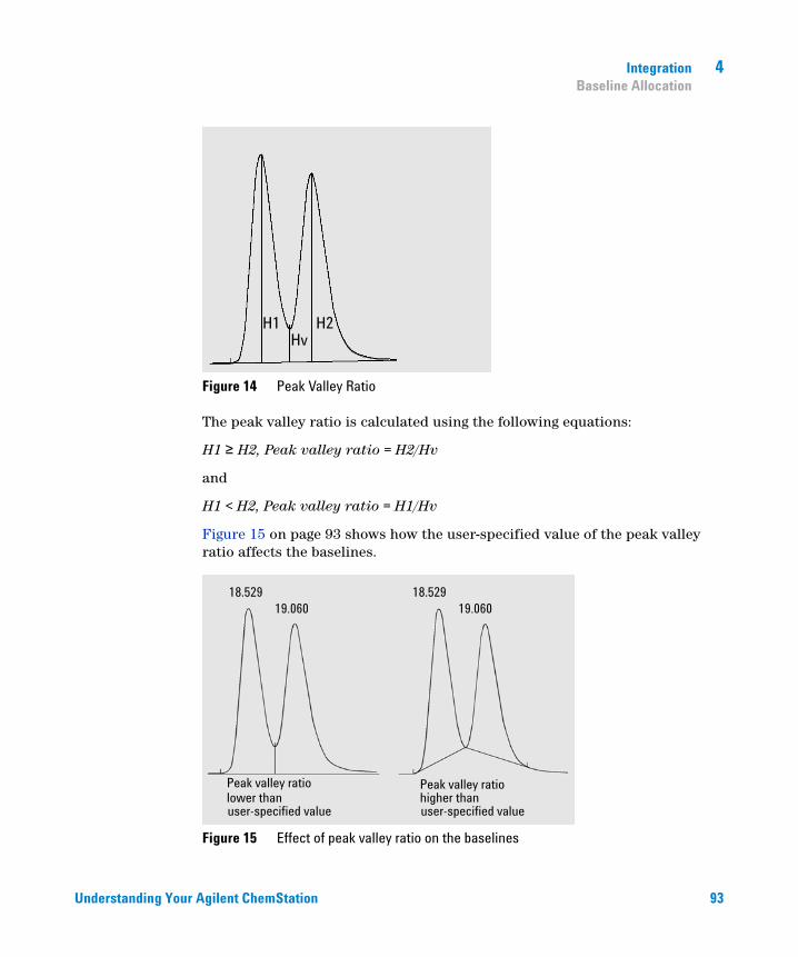
Understanding Your Agilent ChemStation 93
Integration 4Baseline Allocation
Figure 14 Peak Valley Ratio
The peak valley ratio is calculated using the following equations:
H1 ≥ H2, Peak valley ratio = H2/Hv
and
H1 < H2, Peak valley ratio = H1/Hv
Figure 15 on page 93 shows how the user-specified value of the peak valley ratio affects the baselines.
Figure 15 Effect of peak valley ratio on the baselines

94 Understanding Your Agilent ChemStation
4 IntegrationBaseline Allocation
Tangent Skimming
Tangent skimming is a form of baseline constructed for peaks found on the upslope or downslope of a peak. When tangent skimming is enabled, four models are available to calculate suitable peak areas:
• exponential curve fitting,
• new exponential skim
• straight line skim,
• combined exponential and straight line calculations for the best fit (standard skims).
Exponential Curve Fitting
This skim model draws a curve using an exponential equation through the start and end of the child peak (the height of the start of the child peak is corrected for the parent peak slope). The curve passes under each child peak that follows the parent peak; the area under the skim curve is subtracted from the child peaks and added to the parent peak (see Figure 17 on page 95).
Figure 16 Exponential skim
New Mode Exponential Curve Fitting
This skim model draws a curve using an exponential equation to approximate the leading or trailing edge of the parent peak. The curve passes under one or more peaks that follow the parent peak (child peaks). The area under the skim curve is subtracted from the child peaks and added to the main peak. More than one child peak can be skimmed using the same exponential model; all

Understanding Your Agilent ChemStation 95
Integration 4Baseline Allocation
peaks after the first child peak are separated by drop lines, beginning at the end of the first child peak, and are dropped only to the skim (see Figure 17 on page 95).
Figure 17 New mode exponential skim
Straight Line Skim
This skim model draws a straight line through the start and end of a child peak. The height of the start of the child peak is corrected for the parent peak slope. The area under the straight line is subtracted from the child peak and added to the parent peak (see Figure 18 on page 95).
Figure 18 Straight line skim

96 Understanding Your Agilent ChemStation
4 IntegrationBaseline Allocation
Standard Skims
The appropriate calculation is chosen for a particular application; by default, the chosen method is a combination of exponential and straight line calculations for the best fit.
The switch from an exponential to a linear calculation is performed in a way that eliminates abrupt discontinuities of heights or areas.
• When the signal is well above the baseline, the tail-fitting calculation is exponential.
• When the signal is within the baseline envelope, the tail fitting calculation is a straight line.
The combination calculations are reported as exponential or tangent skim.
Skim Criteria
Two criteria determine whether a skim line is used to calculate the area of a child peak eluting on the trailing edge of a parent peak:
• tail skim height ratio
• valley height ratio
These criteria are not used if a timed event for an exponential is in effect, or if the parent peak is itself a child peak. The separation code between parent peak and child peak must be of type Valley.
Tail Skim Height Ratio is the ratio of the baseline-corrected height of the parent peak (Hp in Figure 19 on page 96) to the baseline-corrected height of the child peak (Hc). This ratio must be greater than the specified value for the child peak to be skimmed.
Figure 19 Skim criteria
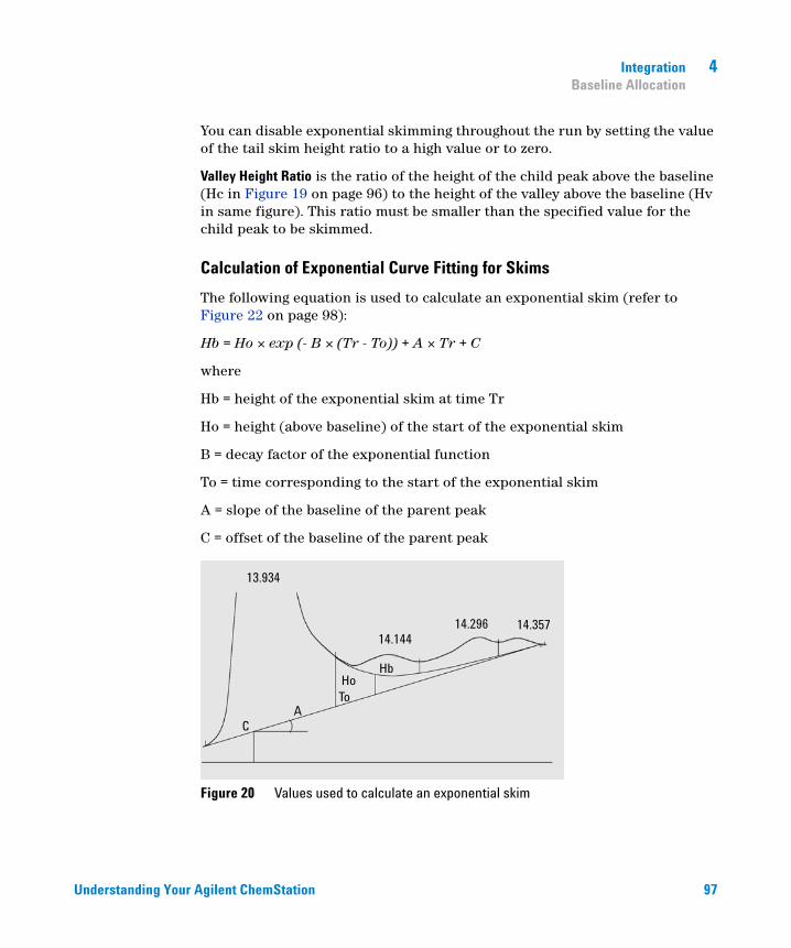
Understanding Your Agilent ChemStation 97
Integration 4Baseline Allocation
You can disable exponential skimming throughout the run by setting the value of the tail skim height ratio to a high value or to zero.
Valley Height Ratio is the ratio of the height of the child peak above the baseline (Hc in Figure 19 on page 96) to the height of the valley above the baseline (Hv in same figure). This ratio must be smaller than the specified value for the child peak to be skimmed.
Calculation of Exponential Curve Fitting for Skims
The following equation is used to calculate an exponential skim (refer to Figure 22 on page 98):
Hb = Ho × exp (- B × (Tr - To)) + A × Tr + C
where
Hb = height of the exponential skim at time Tr
Ho = height (above baseline) of the start of the exponential skim
B = decay factor of the exponential function
To = time corresponding to the start of the exponential skim
A = slope of the baseline of the parent peak
C = offset of the baseline of the parent peak
Figure 20 Values used to calculate an exponential skim

98 Understanding Your Agilent ChemStation
4 IntegrationBaseline Allocation
The exponential model is fitted through the part of the tail of the parent peak immediately before the first child peak. Figure 21 on page 98 shows the corrected curve of a child peak after tangent skimming.
Figure 21 Tail-corrected child peak
Front Peak Skimming
As for child peaks on the tail of a parent peak, special integration is required for some peaks on the front/upslope of a peak, see Figure 22 on page 98.
Figure 22 Front peak skimming
Front peak skimmimg is treated the same way as tail peak skimming, using the same skim models.
The skim criteria are:
• front skim height ratio
• valley height ratio
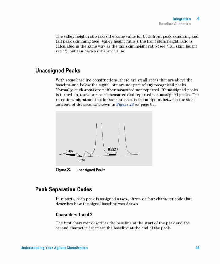
Understanding Your Agilent ChemStation 99
Integration 4Baseline Allocation
The valley height ratio takes the same value for both front peak skimming and tail peak skimming (see "Valley height ratio"); the front skim height ratio is calculated in the same way as the tail skim height ratio (see "Tail skim height ratio"), but can have a different value.
Unassigned Peaks
With some baseline constructions, there are small areas that are above the baseline and below the signal, but are not part of any recognized peaks. Normally, such areas are neither measured nor reported. If unassigned peaks is turned on, these areas are measured and reported as unassigned peaks. The retention/migration time for such an area is the midpoint between the start and end of the area, as shown in Figure 23 on page 99.
Figure 23 Unassigned Peaks
Peak Separation Codes
In reports, each peak is assigned a two-, three- or four-character code that describes how the signal baseline was drawn.
Characters 1 and 2
The first character describes the baseline at the start of the peak and the second character describes the baseline at the end of the peak.

100 Understanding Your Agilent ChemStation
4 IntegrationBaseline Allocation
B The peak started or stopped on the baseline.
V The peak started or stopped with a valley drop-line.
P The peak started or stopped while the baseline was penetrated.
H The peak started or stopped on a forced horizontal baseline.
F The peak started or stopped on a forced point.
M The peak was manually integrated.
U The peak was unassigned.
Additional flags may also be appended (in order of precedence):
Character 3
D The peak was distorted.
A The integration was aborted.
U An under-range condition occurred.
O An over-range condition occurred.
Character 4
The fourth character describes the peak type:
S The peak is a solvent peak.
N The peak is a negative peak.
+ The peak is an area summed peak.
T Tangent-skimmed peak (standard skim).
X Tangent-skimmed peak (old mode exponential skim).
E Tangent-skimmed peak (new mode exponential skim).
m Peak defined by manual baseline.
n Negative peak defined by manual baseline.
t Tangent-skimmed peak defined by manual baseline.
R The peak is a recalculated solvent peak.

Understanding Your Agilent ChemStation 101
Integration 4Baseline Allocation
f Peak defined by a front shoulder tangent.
b Peak defined by a rear shoulder tangent.
F Peak defined by a front shoulder drop-line.
B Peak defined by a rear shoulder drop-line.
U The peak is unassigned.

102 Understanding Your Agilent ChemStation
4 IntegrationPeak Area Measurement
Peak Area Measurement
The final step in peak integration is determining the final area of the peak.
Peak areas are calculated from the contents of the cardinal point file. Cardinal points are the points chosen by the integrator to define and quantify a peak (see “Identifying the Cardinal Points of a Peak” on page 76). These include baseline points, valley points, peak apex, points at peak half height. Cardinal points have a horizontal coordinate of elapsed time, a vertical coordinate of height from the baseline, area, and other parameters that the integrator uses to calculate the peak areas.
Figure 24 Area measurement for Baseline-to-Baseline Peaks
In the case of a simple, isolated peak, the peak area is determined by the accumulated area above the baseline between peak start and stop (identified by tick marks).
Determination of the area
The area that the integrator calculates during integration is determined as follows:
• for baseline-to-baseline (BB) peaks, the area above the baseline between the tick marks, as in Figure 24 on page 102,

Understanding Your Agilent ChemStation 103
Integration 4Peak Area Measurement
• for valley-to-valley (VV) peaks, the area above the baseline, segmented with vertical dropped lines from tick marks, as in Figure 25 on page 103,
Figure 25 Area Measurement for Valley-to-Valley Peaks
• for tangent (T) peaks, the area above the reset baseline,
• for solvent (S) peaks, the area above the horizontal extension from the last-found baseline point and below the reset baseline given to tangent (T) peaks. A solvent peak may rise too slowly to be recognized, or there may be a group of peaks well into the run which you feel should be treated as a solvent with a set of riders. This usually involves a merged group of peaks where the first one is far larger than the rest. The simple drop-line treatment would exaggerate the later peaks because they are actually sitting on the tail of the first one. By forcing the first peak to be recognized as a solvent, the rest of the group is skimmed off the tail,
• negative peaks that occur below the baseline have a positive area, as shown in Figure 26 on page 104.

104 Understanding Your Agilent ChemStation
4 IntegrationPeak Area Measurement
Figure 26 Area Measurement for Negative Peaks
Units and Conversion Factors
Externally, the data contains a set of data points; they can be either sampled data or integrated data. In the case of integrated data, each data point corresponds to an area, which is expressed as Height × Time. In the case of sampled data, each data point corresponds to a height.
Therefore, in the case of integrated data, height is a calculated entity, obtained by dividing area by the time elapsed since the preceding data point. In the case of sampled data, area is calculated by multiplying the data by the time elapsed since the preceding data point.
The integration calculation makes use of both entities. The units carried internally inside the integrator are: counts × milliseconds for area and counts for height. This is done to provide a common base for integer truncations when needed. The measurements of time, area and height are reported in real physical units, irrespective of how they are measured, calculated and stored in the software.
Understanding Your Agilent ChemStation 105
Integration 4Integration Events
Integration Events
The integrator provides you with a number of initial and timed integrator events. Many events are on/off or start/stop pairs.
Initial Events
Initial Peak Width Initial peak width sets the integrator’s internal peak width to this value for the start of run. This initial peak width is used to scale the accumulator that detects peak up-slope, down-slope, and tailing. The integrator updates the peak width when necessary during the run to optimize the integration. You specify the peak width in units of time that correspond to the peak width at half-height of the first expected peak (excluding the solvent peak).
Slope Sensitivity Slope sensitivity is the setting for peak sensitivity. This is a setting that changes on a linear scale.
Height reject Height reject sets peak rejection by final height. Any peaks that have heights less than the minimum height are not reported.
Area reject Area reject sets peak rejection by final area. Any peaks that have areas less than the minimum area are not reported.
Shoulderdetection
When shoulder detection is on, the integrator detects shoulders using the curvature of the peak as given by the second derivative. When the curvature goes to zero, the integrator identifies this point of inflection as a possible shoulder. If the integrator identifies another point of inflection before the apex of the peak, a shoulder has been detected.
Peak Width
The peak width setting controls the selectivity of the integrator to distinguish peaks from baseline noise. To obtain good performance, the peak width must be set close to the width at half-height of the actual chromatographic/electropherographic peaks. The integrator updates the peak width when necessary during the run to optimize the integration.

106 Understanding Your Agilent ChemStation
4 IntegrationIntegration Events
Choosing Peak Width
Choose the setting that provides just enough filtering to prevent noise being interpreted as peaks without distorting the information in the signal.
• To choose a suitable initial peak width for a single peak of interest, use the peak’s time width as the base as a reference.
• To choose a suitable initial peak width when there are multiple peaks of interest, set the initial peak width to a value equal to or less than the narrowest peak width to obtain optimal peak selectivity.
If the selected initial peak width is too low, noise may be interpreted as peaks. If broad and narrow peaks are mixed, you may decide to use runtime programmed events to adjust the peak width for certain peaks. Sometimes, peaks become significantly broader as the analysis progresses, for example in isothermal GC and isocratic LC analyses. To compensate for this, the integrator automatically updates the peak width as peaks broaden during an analysis unless disabled or set with a timed event.
The Peak Width update is weighted in the following way:
0,75 × (existing peak width) + 0,25 × (width of current peak)
If a timed integration event disables or sets the peak width to a specific value, the automatic peak width adjustment is disabled.
Height Reject and Peak Width
Both peak width and height reject are very important in the integration process. You can achieve different results by changing these values.
• Increase both the height reject and peak width where relatively dominant components must be detected and quantified in a high-noise environment. An increased peak width improves the filtering of noise and an increased height reject ensures that random noise is ignored.
• Decrease height reject and peak width to detect and quantify trace components, those whose heights approach that of the noise itself. Decreasing peak width decreases signal filtering, while decreasing height reject ensures that small peaks are not rejected because they have insufficient height.
• When an analysis contains peaks with varying peak widths, set peak width for the narrower peaks and reduce height reject to ensure that the broad peaks are not ignored because of their reduced height.

Understanding Your Agilent ChemStation 107
Integration 4Integration Events
Tuning Integration
It is often useful to change the values for the slope sensitivity, peak width, height reject, and area reject to customize integration.
Figure 27 on page 107 shows how these parameters affect the integration of five peaks in a signal.
Figure 27 Using Initial Events
A peak is integrated only when all of the four integration parameters are satisfied. Using the peak width for peak 3, the area reject and slope sensitivity shown in Figure 27 on page 107, only peaks 1, 3, 5 and 7 are integrated.
Peak 1 is integrated as all four integration parameters are satisfied.
Peak 2 is rejected because the area is below the set area reject value.
Peak 3 is integrated as all four integration parameters are satisfied.
Peak 4 is not integrated because the peak height is below the Height Reject.
Peak 5 is rejected because the area is below the set area reject value.
Peak 6 is not integrated; filtering and bunching make the peak invisible.
Peak 7 is integrated.

108 Understanding Your Agilent ChemStation
4 IntegrationIntegration Events
Timed Events
You can use timed events to customize signal baseline construction when default construction is not appropriate. These events can be useful for summing final peak areas and for correcting short- and long-term baseline aberrations. For further information about integration events see “Initial Events” on page 105.
Autointegrate
The Autointegrate function provides a starting point for setting initial events. This is particularly useful when you are implementing a new method. You start with a default integration events table that contains no timed events; you can then optimize the parameters proposed by the Autointegrate function for general use.
Principles of Operation
The Autointegrate function reads the chromatogram data and calculates the optimal values for the initial integration parameters for each signal in the chromatogram object.
The algorithm examines 1% at the start and end of the chromatogram and determines the noise and slope for this part. Noise is determined as 3 times the standard deviation of the linear regression divided by the square root of the percent number of points used in the regression. These values are used to assign appropriate values to the height reject & slope sensitivity for the integration. The algorithm then assigns a temporary value for the peak width, depending on the length of the chromatogram, using 0.5% for LC and 0.3% to
Table 12 Height and Area Reject Values
Integration Parameter Peak 1 Peak 2 Peak 3 Peak 4 Peak 5 Peak 7
Height reject Above Above Above Below Above Above
Area reject Above Below Above Below Below Above
Peak integrated Yes No Yes No No Yes

Understanding Your Agilent ChemStation 109
Integration 4Integration Events
0.2% for GC. The initial area reject is set to zero and a trial integration is performed. The trial is repeated several times if necessary, adjusting the parameters each time until at least 5 peaks are detected or integration is performed with an initial height reject of 0. The trial integration is terminated if the above conditions are not met after 10 trials.
The results of the integration are examined and the peak width is adjusted based on the peak widths of the detected peaks, biasing the calculation towards the initial peaks. The peak symmetry of the detected peaks is used to include only those peaks with symmetry between 0.8 and 1.3 for the peak width calculation. If not enough symmetric peaks are found, this limit is relaxed to minSymmetry/1.5 and maxSymmetry×1.5. The baseline between the peaks is then examined to refine the earlier values of height reject & slope sensitivity. The area reject is set to 90% of the minimum area of the most symmetric peak detected during the trial integration.
The chromatogram is re-integrated using these final values for the integration parameters, and the results of the integration are stored.
Autointegrate Parameters
The following parameters are set by the autointegrate function:
• Initial slope sensitivity
• Initial height
• Initial peak width
• Initial area reject

110 Understanding Your Agilent ChemStation
4 IntegrationManual Integration
Manual Integration
Manual Integration
This type of integration allows you to integrate selected peaks or groups of peaks. Except for the initial area reject value, the software's event integration is ignored within the specified range of manual integration. If one or more of the peaks resulting from manual integration is below the area reject threshold, it is discarded. The manual integration events use absolute time values. They do not adjust for signal drift.
Manual Integration enables you to define the peak start and stop points, and then include the recalculated areas in quantification and reporting. Manually-integrated peaks are labeled in reports with the peak separation code M. It offers the following features:
Draw Baseline Draw Baseline specifies where the baselines are to be drawn for a peak or set of peaks. You can also specify whether peaks in the range given should be automatically separated at all valley points.
Negative Peaks Negative Peaks specifies when to treat any areas below the baseline as negative peaks. You can also specify whether peaks in the range given should be automatically separated at all valley points.
Tangent Skim Tangent Skim calculates the areas of peaks tangentially skimmed off a main peak. The area of the tangent skimmed peak is subtracted from the area of the main peak.
Split Peak Split Peak specifies a point where to split a peak with a drop-line.
Delete Peak(s) Delete Peak(s) deletes one or more peaks from the integration results.
Peak Separation Codes for Manually-Integrated Peaks
Manually-integrated peaks are labeled in the integration reports by the peak code MM.
If there is a peak before the manually-integrated peak, and the end of this peak changes because of the manual integration, it is given the code F (forced).
A solvent peak which has been affected by manual integration, such as tangent skim, are labeled R (re-calculated solvent).

Understanding Your Agilent ChemStation 111
Integration 4Manual Integration
Saving Manual Integration Events
Manual integration events, e.g. a manually drawn baseline, are even more data file specific than timed integration events. In case of complicated chromatograms, it is highly desirable to be able to use these events for reprocessing. Therefore, starting with ChemStation B.04.01, manual integration events can be stored directly in the data file instead of the method.
Each time the data file is reviewed or reprocessed, the manual events in the data file are automatically applied. A run containing manual integration events is marked in the Navigation Table in the corresponding column.
In addition to the tools for drawing a baseline and deleting a peak manually, three additional tools are available in the user interface to
• Save manual events of the currently shown chromatograms into the data file,
• Remove all events from the currently shown chromatograms,
• Undo the last manual integration events (available until the event is saved).
When continuing to the next data file during review in the Navigation Table, ChemStation will check for unsaved manual integration events and ask the user whether he wants to save the events.
Manual events stored in the data file during review in the Navigation Table do not interfere with manual integration events stored during review in the Batch mode. These two ways of review are completely separated with regard to the manual events of a data file.
In ChemStation revisions prior to B.04.01, manual integration events were stored in the method instead of the individual data file. In B.04.01, this workflow can still be used. The Integration menu in Data Analysis view provides the following items in order to handle manual integration events with the method:
• Update Manual Events of Method: Save newly drawn manual events to the method.
• Apply Manual Events from Method: Apply the manual events currently saved in the method to the currently loaded data file.
• Remove Manual Events from Method: Delete the manual events from the method.

112 Understanding Your Agilent ChemStation
4 IntegrationManual Integration
In order to convert manual events stored in a method to storage in the data file, apply the events from the method and store the results in the data file. If wanted, remove the events from the method.
In case the Manual Events checkbox of the Integration Events Table of a method is enabled, the manual events of the method are always applied when loading a data file using this method. If the data file contains additional manual events, they are applied after the events of the method. When the Manual Events checkbox is enabled, the user is never asked to save the events to the data file.
In order to convert manual events stored in a method to storage in the data file, apply the events from the method and store the results in the data file. You may remove the events from the method now.
In case the Manual Events checkbox of the Integration Events Table of a method is enabled, the manual events of the method are always applied when loading a data file using this method. If the data file contains additional manual events, they are applied after the events of the method. When the Manual Events checkbox is enabled, the user is never asked to save the events to the data file.
Conversion of Manual Integration Events Saved in a Method
In ChemStation revisions prior to B.04.01, manual integration events were stored in the method instead of the individual data file. In order to store the manual events in a data file specific way, it was most convIn order to store the manual events in a data file specific way, it was most convienient to use the individualenient to use the individual method DA.M of each specific data file.
The Integration menu in Data Analysis view provides the following items in order to either convert manual integration events in the method to events stored in the data file, or to continue to work with manual events stored in the method:
• Update Manual Events of Method: Save newly drawn manual events to the method.
• Apply Manual Events from Method: Apply the manual events currently saved in the method to the currently loaded data file.
• Remove Manual Events from Method: Delete the manual events from the method.
113
Understanding Your Agilent ChemStation
Agilent Technologies
5Quantification
What is Quantification? 114
Quantification Calculations 115
Correction Factors 116
Absolute Response Factor 116
Multiplier 116
Dilution Factor 116
Sample Amount 117
Uncalibrated Calculation Procedures 118
Area% and Height% 118
Calibrated Calculation Procedures 119
ESTD Calculation 120
Norm% Calculation 122
ISTD Calculation 123
Run 1: Calibration 124
Run 2: Unknown Sample 124
ISTD Calculation of Calibrated Peaks 125
ISTD Calculation of Uncalibrated Peaks 125
This chapter describes how ChemStation does quantification. It gives details on area% and height% calculations, external standard (ESTD) calculation, norm% calculation, internal standard (ISTD) calculation, and quantification of unidentified peaks.

114 Understanding Your Agilent ChemStation
5 QuantificationWhat is Quantification?
What is Quantification?
After the peaks have been integrated and identified, the next step in the analysis is quantification. Quantification uses peak area or height to determine the concentration of a compound in a sample.
A quantitative analysis involves many steps which are briefly summarized as follows:
• Know the compound you are analyzing.
• Establish a method for analyzing samples containing this compound.
• Analyze a sample or samples containing a known concentration or concentrations of the compound to obtain the response due to that concentration.
You may alternatively analyze a number of these samples with different concentrations of the compounds of interest if your detector has a non-linear response. This process is referred to as multi-level calibration.
• Analyze the sample containing an unknown concentration of the compound to obtain the response due to the unknown concentration.
• Compare the response of the unknown concentration to the response of the known concentration to determine how much of the compound is present.
To obtain a valid comparison for the unknown sample response to that of the known sample, the data must be acquired and processed under identical conditions.

Understanding Your Agilent ChemStation 115
Quantification 5Quantification Calculations
Quantification Calculations
The ChemStation offers the following calculation procedures for determining the concentration of each component present in a mixture:
• Percent
• Normalization
• External standard (ESTD)
• ESTD%
• Internal standard (ISTD)
• ISTD%
The calculations used to determine the concentration of a compound in an unknown sample depend on the type of quantification. Each calculation procedure uses the peak area or height for the calculation and produces a different type of report.

116 Understanding Your Agilent ChemStation
5 QuantificationCorrection Factors
Correction Factors
The quantification calculations use four correction factors, the absolute response factor, the multiplier, the dilution factor, and the sample amount. These factors are used in the calibration procedures to compensate for variations in detector response to different sample components, concentrations, sample dilutions, sample amounts, and for converting units.
Absolute Response Factor
The absolute response factor for a sample component represents the amount of the component divided by the measured area or height of the component’s peak in the analysis of a calibration mixture. The absolute response factor, which is used by each calibrated calculation procedure, corrects for detector response to individual sample components.
Multiplier
The multiplier is used in each calculation formula to multiply the result for each component. The multiplier may be used to convert units to express amounts.
Dilution Factor
The dilution factor is a number by which all calculated results are multiplied before the report is printed. You can use the dilution factor to change the scale of the results or correct for changes in sample composition during pre-analysis work. You can also use the dilution factor for any other purposes that require the use of a constant factor.

Understanding Your Agilent ChemStation 117
Quantification 5Correction Factors
Sample Amount
If the ESTD% or ISTD% calculations are selected, the ESTD and ISTD reports give relative values rather than absolute values, that is, the amount of each component is expressed as a percentage of the sample amount. The sample amount is used in ESTD% and ISTD% reports to convert the absolute amount of the components analyzed to relative values by dividing by the value specified.

118 Understanding Your Agilent ChemStation
5 QuantificationUncalibrated Calculation Procedures
Uncalibrated Calculation Procedures
Uncalibrated calculation procedures do not require a calibration table.
Area% and Height%
The Area% calculation procedure reports the area of each peak in the run as a percentage of the total area of all peaks in the run. Area% does not require prior calibration and does not depend upon the amount of sample injected within the limits of the detector. No response factors are used. If all components respond equally in the detector and are eluted, then Area% provides a suitable approximation of the relative amounts of components.
Area% is used routinely where qualitative results are of interest and to produce information to create the calibration table required for other calibration procedures.
The Height% calculation procedure reports the height of each peak in the run as a percentage of the total height of all peaks in the run.
The multiplier and dilution factor from the Calibration Settings, from the Sample Information dialog box, or from the Sequence Table are not applied in Area% or Height% calculation.

Understanding Your Agilent ChemStation 119
Quantification 5Calibrated Calculation Procedures
Calibrated Calculation Procedures
The external standard (ESTD), normalization, and internal standard (ISTD) calculation procedures require response factors and therefore use a calibration table. The calibration table specifies conversion of responses into the units you choose by the procedure you select.

120 Understanding Your Agilent ChemStation
5 QuantificationESTD Calculation
ESTD Calculation
The ESTD procedure is the basic quantification procedure in which both calibration and unknown samples are analyzed under the same conditions. The results from the unknown sample are then compared with those of the calibration sample to calculate the amount in the unknown.
The ESTD procedure uses absolute response factors unlike the ISTD procedure. The response factors are obtained from a calibration and then stored. In following sample runs, component amounts are calculated by applying these response factors to the measured sample amounts. Make sure that the sample injection size is reproducible from run to run, since there is no standard in the sample to correct for variations in injection size or sample preparation.
When preparing an ESTD report, the calculation of the amount of a particular compound in an unknown sample occurs in two steps:
1 An equation for the curve through the calibration points for this compound is calculated using the type of fit specified in the Calibration Settings or Calibration Curve dialog box.
2 The amount of the compound in the unknown is calculated using the equation described below. This amount may appear in the report or it may be used in additional calculations called for by Multiplier, Dilution Factor, or Sample Amount values before being reported.
If the ESTD report is selected, the equation used to compute the absolute amount of component x is:
where:
Responsex is the response of peak x;
RFx is the response factor for component x, calculated as:
M is the multiplier.
D is the dilution factor.

Understanding Your Agilent ChemStation 121
Quantification 5ESTD Calculation
Figure 28 Response Factor
The multiplier and dilution factor are read either from the Calibration Settings or from the Sample Information dialog box.
If the ESTD% report is selected and sample amount is not zero, the relative amount (%) of a component x is calculated as shown below:
where:
Absolute amount of x is calculated as shown above in the ESTD calculation;
Sample amount is obtained from the Sample Information box, or from the Calibration Settings dialog box for single runs. If sample amount is zero, the ESTD is calculated.

122 Understanding Your Agilent ChemStation
5 QuantificationNorm% Calculation
Norm% Calculation
In the normalization method, response factors are applied to the peak areas (or heights) to compensate for changes that occur in detector sensitivity for the different sample components.
The Norm% report is calculated in the same way as an ESTD report except that there is an additional step to calculate the relative rather than absolute amounts of compounds.
The Norm% report has the same disadvantage as the Area% and Height% reports. Any changes that affect the total peak area will affect the concentration calculation of each individual peak. The normalization report should only be used if all components of interest are eluted and integrated. Excluding selected peaks from a normalization report will change the reported results in the sample.
The equation used to calculate the Norm% of a component x is:
where:
The multiplier and dilution factor are read either from the Calibration Settings, from the Sample Information dialog box or from the Sequence Table.
Responsex is the area (or height) of peak x,
RFx is the response factor,
Σ (Response · RF) is the total of all the (Response · RF) products for all peaks including peak x,
M is the multiplier,
D is the dilution factor.

Understanding Your Agilent ChemStation 123
Quantification 5ISTD Calculation
ISTD Calculation
The ISTD procedure eliminates the disadvantages of the ESTD method by adding a known amount of a component which serves as a normalizing factor. This component, the internal standard, is added to both calibration and unknown samples.
The software takes the appropriate response factors obtained from a previous calibration stored in the method. Using the internal standard concentration and peak areas or heights from the run, the software calculates component concentrations.
The compound used as an internal standard should be similar to the calibrated compound, both chemically and in retention/migration time, but it must be chromatographically distinguishable.
If the ISTD procedure is used for calibrations with a non-linear characteristic, care must be taken that errors which result from the calculation principle do not cause systematic errors. In multi-level calibrations, the amount of the ISTD compound should be kept constant, i.e. the same for all levels if the calibration curve of the compound is non-linear.
In the internal standard analysis, the amount of the component of interest is related to the amount of the internal standard component by the ratio of the responses of the two peaks.
In a two-run ISTD calibration, the calculation of the corrected amount ratio of a particular compound in an unknown sample occurs in the following stages:
Table 13 ISTD Procedure
Advantages Disadvantages
Sample-size variation is not critical.
Instrument drift is compensated by the internal standard.
The effects of sample preparations are minimized if the chemical behavior of the ISTD and unknown are similar.
The internal standard must be added to every sample.

124 Understanding Your Agilent ChemStation
5 QuantificationISTD Calculation
Run 1: Calibration
1 The calibration points are constructed by calculating an amount ratio and a response ratio for each level of a particular peak in the calibration table.
The amount ratio is the amount of the compound divided by the amount of the internal standard at this level.
The response ratio is the area of the compound divided by the area or height of the internal standard at this level.
2 An equation for the curve through the calibration points is calculated using the type of curve fit specified in the Calibration Settings dialog box or Calibration Curve dialog box.
Figure 29 Amount Ratio
Run 2: Unknown Sample
1 The response of the compound in the unknown sample is divided by the response of the internal standard in the unknown sample to give a response ratio for the unknown.
2 An amount ratio for the unknown is calculated using the curve fit equation determined in step 2 above, and the actual amount of ISTD in the sample.
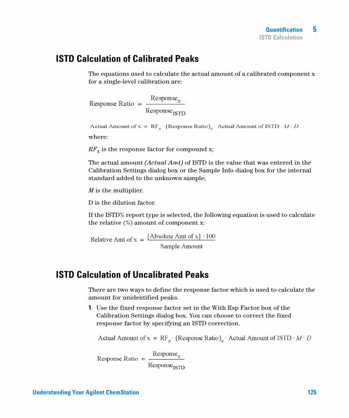
Understanding Your Agilent ChemStation 125
Quantification 5ISTD Calculation
ISTD Calculation of Calibrated Peaks
The equations used to calculate the actual amount of a calibrated component x for a single-level calibration are:
where:
RFx is the response factor for compound x;
The actual amount (Actual Amt) of ISTD is the value that was entered in the Calibration Settings dialog box or the Sample Info dialog box for the internal standard added to the unknown sample;
M is the multiplier.
D is the dilution factor.
If the ISTD% report type is selected, the following equation is used to calculate the relative (%) amount of component x:
ISTD Calculation of Uncalibrated Peaks
There are two ways to define the response factor which is used to calculate the amount for unidentified peaks.
1 Use the fixed response factor set in the With Rsp Factor box of the Calibration Settings dialog box. You can choose to correct the fixed response factor by specifying an ISTD correction.
126 Understanding Your Agilent ChemStation
5 QuantificationISTD Calculation
RFx is the Response Factor set in the Calibration Settings dialog box.
You can see from these formulae that the variations in the ISTD response are used to correct the quantification of the unknown component.
2 Use a calibrated peak. This ensures that the same response factor is used for the quantification of all peaks. The response factor of the selected compound and the uncalibrated peaks is corrected during all recalibrations. If the calibrated peak response factor changes, then the response factor for the unidentified peaks also changes by the same amount. If a Calibration Table is already set up, you can select a compound from the Using Compound combo box in the Calibration Settings dialog box.
The equations used to calculate the actual amount of an uncalibrated peak x are shown above.
127
Understanding Your Agilent ChemStation
Agilent Technologies
6Peak Identification
What is Peak Identification? 128
Peak Matching Rules 129
Types of Peak Identification 130
Absolute Retention/Migration Time 130
Corrected Retention/Migration Time 130
Peak Qualifiers 130
Amount Limits 131
Absolute Retention/Migration Time 132
Corrected Retention/Migration Times 134
Single Reference Peaks 134
Multiple Reference Peaks 134
Peak Qualifiers 136
Signal Correlation 137
Qualifier Verification 137
Qualifier Ratio Calculation 137
The Identification Process 139
Finding the Reference Peaks 139
Finding the ISTD Peaks 139
Finding the Remaining Calibrated Peaks 140
Classification of Unidentified Peaks 140
This chapter describes the concepts of peak identification.
128 Understanding Your Agilent ChemStation
6 Peak IdentificationWhat is Peak Identification?
What is Peak Identification?
Peak identification identifies the components in an unknown sample based on their chromatographic/electropherographic characteristics determined by the analysis of a well-defined calibration sample.
The identification of these components is a necessary step in quantification if the analytical method requires quantification. The signal characteristics of each component of interest are stored in the calibration table of the method.
The function of the peak identification process is to compare each peak in the signal with the peaks stored in the calibration table.
The calibration table contains the expected retention/migration times of components of interest. A peak that matches the retention/migration time of a peak in the calibration table is given the attributes of that component, for example, the name and response factor. Peaks that do not match any of the peaks in the calibration table are classified as unknown. The process is controlled by:
• the retention/migration time in the calibration table for peaks designated as time reference peaks,
• the retention/migration time windows specified for reference peaks,
• the retention/migration times in the calibration table for the calibrated peaks that are not time reference peaks,
• the retention/migration time window specified for these non-reference peaks, and
• the presence of any additional qualifying peaks in the correct ratios.
Understanding Your Agilent ChemStation 129
Peak Identification 6Peak Matching Rules
Peak Matching Rules
The following rules apply to the peak matching process:
• if a sample peak falls within the peak matching window of a component peak from the calibration table, the peak is given the attributes of that component,
• if more than one sample peak falls within the peak matching window, then, the peak closest to the expected retention/migration time is identified as that component,
• if a peak is a time reference or internal standard, then the largest peak in the window is identified as that component,
• if peak qualifiers are also used then the peak ratio is used in combination with the peak matching window to identify the component peak,
• if the peak is a qualifier peak, the measured peak closest to the main peak of the compound is identified, and
• if a sample peak does not fall in any peak matching window, it is listed as an unknown component.

130 Understanding Your Agilent ChemStation
6 Peak IdentificationTypes of Peak Identification
Types of Peak Identification
There are different techniques that can be used to match sample peaks with those in the calibration table of the ChemStation software.
Absolute Retention/Migration Time
The retention/migration time of the sample peak is compared with the expected retention/migration time specified for each component in the calibration table.
Corrected Retention/Migration Time
The expected retention/migration times of component peaks are corrected using the actual retention/migration times of one or more reference peaks, and the matching process is done using these corrected (relative) retention/migration times. The reference peak or peaks must be specified in the calibration table.
Peak Qualifiers
In addition to identifying peaks by retention/migration time, you can use peaks qualifiers to allow a more precise result. If more than one peak occurs in a retention/migration time window then qualifiers should be used to identify the correct compound.

Understanding Your Agilent ChemStation 131
Peak Identification 6Types of Peak Identification
Amount Limits
The amount limits defined in the Compound Details dialog box are used to qualify the peak identification. If the amount of the identified compound is inside the amount limits the peak identification is indicated in the report.

132 Understanding Your Agilent ChemStation
6 Peak IdentificationAbsolute Retention/Migration Time
Absolute Retention/Migration Time
A retention/migration time window is used in the peak matching process. The retention/migration time window is a window which is centered on the retention/migration time for an expected peak. Any sample peak that falls within this window may be considered as a candidate for component identification.
Figure 30 on page 132 shows a retention/migration time window for peak 2 which is between 1.809 and 2.631 minutes where the expected retention/migration time is 2.22 minutes. There are two possibilities for peak 2. One is at 1.85 minutes and the other at 2.33 minutes. If the expected peak is a non-reference peak, the peak closest to the expected retention/migration time of 2.22 minutes is selected.
If the expected peak is a time reference or internal standard, the largest peak in the window is selected.
In both cases the ChemStation selects the peak at 2.33 minutes. If the two peaks were the same size then the peak closest to the center of the window is chosen.
Figure 30 Retention/Migration Time Windows
Three types of windows are used when trying to locate peaks.
• reference peak windows which apply to reference peaks only,
• non-reference peak windows which apply to all other calibrated peaks, and
• specific window values for individual components which are set in the Compound Details dialog box.

Understanding Your Agilent ChemStation 133
Peak Identification 6Absolute Retention/Migration Time
The default values for these windows are entered in the Calibration Settings dialog box. The width on either side of the retention/migration time that defines the peak matching window is the sum of the absolute and percentage windows.
A window of 5 % means the peak must have a retention/migration time between less than 2.5 % and more than 2.5 % of the calibrated retention/migration time for that peak. For example, a peak with a retention/migration time of 2.00 in the calibration run must appear between 1.95 and 2.05 minutes in subsequent runs.
For example, an absolute window of 0.20 minutes and a relative window of 10 % gives a retention/migration time window of between 1.80 and 2.20 minutes.
1.80 min = 2.00 min - 0.10 min (0.20 min / 2) - 0.10 min (10 % of 2.00 min).
2.20 min = 200 min + 0.10 min (0.20 min / 2) + 0.10 min (10 % of 2.00 min).

134 Understanding Your Agilent ChemStation
6 Peak IdentificationCorrected Retention/Migration Times
Corrected Retention/Migration Times
To match peaks by absolute retention/migration times may be simple but not always reliable. Individual retention/migration times may vary slightly due to a small change in conditions or technique. As a result peaks may occur outside the peak matching windows and therefore are not identified.
A technique to deal with the inevitable fluctuations that occur in absolute retention/migration times is to express component retention/migration times relative to one or more reference peaks.
Reference peaks are identified in the calibration table with an entry in the reference column for that peak. The relative peak matching technique uses the reference peak or peaks to modify the location of the peak matching windows in order to compensate for shifts in the retention/migration times of sample peaks.
If no reference peak is defined in the method or the ChemStation cannot identify at least one reference peak during the run, the software will use absolute retention/migration times for identification.
Single Reference Peaks
A retention/migration time window for the reference peak is created around its retention/migration time. The largest peak falling within this window is identified as the reference peak. The expected retention/migration times of all other peaks in the calibration table are corrected, in proportion to the ratio of the expected retention/migration time to the actual retention/migration time of the reference peak.
Multiple Reference Peaks
Correcting retention/migration times with a single reference peak is based on the assumption that the deviation of actual retention/migration time from the expected retention/migration times changes uniformly and linearly as the run

Understanding Your Agilent ChemStation 135
Peak Identification 6Corrected Retention/Migration Times
progresses. Often during a long run the retention/migration time changes non-uniformly. In such cases better results are obtained using multiple reference peaks spaced at intervals across the run. This splits the signal into separate zones. Within each zone the deviation between retention/migration times is assumed to change linearly, but the rate of change is determined separately for each zone.
NOTE The time correction algorithm may fail if the retention times of multiple reference peaks are too close to each other and are not distributed across the total run time.

136 Understanding Your Agilent ChemStation
6 Peak IdentificationPeak Qualifiers
Peak Qualifiers
A component can be detected with more than one signal. Although applicable to all forms of chromatography using multiple detectors or detectors capable of producing multiple signals, multisignal detection is most commonly used in liquid chromatography with multiple wavelength or diode array detectors. Such detectors are normally set up so that the wavelength closest to the greatest absorbance (area) is used to define the main peak in the calibration table. In Figure 31 on page 136 this is Lambda1.
The two other wavelengths that were acquired as signals can be used as peak qualifiers. In the figure these are Lambda2 and Lambda3.
Figure 31 Peak Qualifiers
Peaks of a compound have a constant response ratio over different wavelengths.
The qualifier peak response is a certain percentage of the main peak response. Limits which determine the acceptable range for the expected response can be set in the calibration table when the Identification Details option is selected. If

Understanding Your Agilent ChemStation 137
Peak Identification 6Peak Qualifiers
the ratio between the main peak qualifier Lambda1 and the qualifier peak, for example, Lambda3 is within the allowed limits then the compound identity can be confirmed.
Signal Correlation
Signal correlation means that two peaks measured in different detector signals within a defined time window are assigned to the same compound. The signal correlation window can be controlled by the SignalCorrWin parameter in the QuantParm table of the _DaMethod register. Signal correlation is disabled when setting the signal correlation window to 0.0 minutes (see the Macro Programming Guide for more information). When signal correlation is off, peaks eluting at the same retention/migration time in different detector signals are treated as different compounds.
The default signal correlation window for LC, CE, CE/MS and LC/MS data is 0.03 minutes and 0.0 minutes for GC data.
Qualifier Verification
If signal correlation is enabled, qualifier verification is active for all data file types by default. It can be disabled by setting the UseQualifiers flag in the Quantification Parameters table of the method (see the macro programming guide for more details). Qualifier verification is also disabled when signal correlation is switched off.
Qualifier Ratio Calculation
When qualifiers verification is enabled for a compound, the ratio of the qualifier size and the main peak size is verified against the calibrated limits. The size may be height or area according to the calculation base setting in Specify Report.
The qualifier peaks can be calibrated in the same way as the target compounds. The user does not need to specify the expected qualifier ratio. The expected qualifier ratio is calculated automatically:

138 Understanding Your Agilent ChemStation
6 Peak IdentificationPeak Qualifiers
both measured at the retention time of the compound.
The QualTolerance parameter defines the acceptable range of the qualifier ratio, for example, ± 20%.
The tolerance can be set in the calibration table user interface (Identification Details) and is an absolute percentage.
For multilevel calibrations, the ChemStation calculates a minimum qualifier tolerance based on the measured qualifier ratios at each calibration level. The minimum qualifier tolerance is calculated using the following equation:
where qi is the measured qualifier ratio at level i.

Understanding Your Agilent ChemStation 139
Peak Identification 6The Identification Process
The Identification Process
When attempting to identify peaks, the software makes three passes through the integration data.
Finding the Reference Peaks
The first pass identifies the time reference peaks. The software searches peak retention/migration times from a run for matches within the retention/migration windows of the reference peaks in the calibration table. A peak from the run is identified as a reference peak in the calibration table if the run peak’s retention/migration time is within the window constructed for the calibration table peak.
If more than one peak is found within a window, the peak with the largest area or height followed by a positive signal qualifier match, if set up, is chosen as the reference peak.
After each time reference peak is found, the difference between its retention/migration time and that given in the calibration table is used to adjust the expected retention/migration times of all other peaks in the Calibration table.
Finding the ISTD Peaks
The second pass identifies any defined internal standard peaks. If they have not already been identified as ISTD, peaks may be identified as time reference peaks. ISTD peaks are identified by peak retention/migration time windows and peak qualifiers. If more than one peak is found in the same ISTD window, the largest peak is chosen.

140 Understanding Your Agilent ChemStation
6 Peak IdentificationThe Identification Process
Finding the Remaining Calibrated Peaks
The third pass identifies all remaining peaks listed in the calibration table. The non-reference peaks in the calibration table are matched to the remaining run peaks by using their RT window.
Each non-reference calibrated peak has its own retention/migration time in the calibration table. This is adjusted for the particular run based on the pre-identification of the time reference peaks. The retention/migration time window of the calibrated peak is adjusted based on the corrected retention/migration time of the calibrated peak.
If more than one peak is found in the same window, the peak with a retention/migration time which is closest to the expected retention/migration time and also meets the optional qualifier specifications is chosen.
Classification of Unidentified Peaks
If there are remaining peaks, which are still not identified, they are classified as unknown. The ChemStation attempts to group the unknown peaks that belong to the same compound. If a peak has been detected in more than one signal, the peaks with the same retention/migration time in each signal are grouped to one compound.
Unknown peaks are reported if the corresponding selection has been made in the Calibration Settings dialog box.

141
Understanding Your Agilent ChemStation
Agilent Technologies
7Calibration
Definition of Terms 142
Calibration Table 143
Calibration Curve 144
Unknown Samples 146
Types of Calibration 147
Single-Level Calibration 147
Multilevel Calibration 148
Calibration Ranges 150
Calibration Curve Fits 150
Origin Treatment 150
Group Calibration 153
Peak Summing 154
Recalibration 155
What is Recalibration? 155
Why Recalibrate? 155
Manual Recalibration 155
Recalibrations with Peak Summing 156
Recalibration Options 156
Ways to Recalibrate 157
Recalibration of Unidentified Peaks 157
This chapter describes Calibration in the ChemStation.

142 Understanding Your Agilent ChemStation
7 CalibrationDefinition of Terms
Definition of Terms
Calibration Calibration is the process of determining response factors used to calculate absolute component concentrations by injecting specially prepared calibration samples. The calibration table is also used for identification. See “Peak Identification” on page 127.
Compound A chemical compound can comprise several peaks, in a multiple signal calibration, typically one per signal. In a single signal calibration a compound refers to one peak.
Calibration Level A calibration level comprises the calibration points for one calibration sample concentration. In a multisignal calibration the calibration points can be distributed over several signals.
Calibration Point A calibration point refers to an amount/response ratio for a peak on the calibration curve.
CalibrationSample
A calibration sample, also referred to as a calibration standard or a standard mixture, is a sample containing a known amount of the compound to quantify. In the software the calibration sample is referred to as an injection from the calibration sample vial.
Calibration samples may be purchased from chemical suppliers or they may be prepared using an accurately measured amount of the pure compound. The amount of the compound in the calibration sample is usually expressed as a concentration, typically in ng/µl units.

Understanding Your Agilent ChemStation 143
Calibration 7Calibration Table
Calibration Table
The calibration table specifies conversions of peak areas or heights into the units you choose according to the calculation procedure you select. It contains a list of retention/migration times from a calibration run. These retention/migration times are compared with retention/migration times of peaks from a sample run. Where a match occurs, the peak in the sample is assumed to represent the same component as that in the calibration table, see “Peak Identification” on page 127. During an analysis or while a report is being generated, the amounts entered for each peak are used to calculate the amounts for the calculation procedure selected for the report. The type and amount of information required for creating a calibration table varies with the type of calculation procedure desired.
The following information is needed to create a calibration table:
• the retention/migration time for each calibration mixture component peak, and
• the amount of each component used in making the calibration mixture, expressed in consistent units.

144 Understanding Your Agilent ChemStation
7 CalibrationCalibration Curve
Calibration Curve
A calibration curve is a graphical presentation of the amount and response data for one compound obtained from one or more calibration samples.
Normally an aliquot of the calibration sample is injected, a signal is obtained, and the response is determined by calculating the area or height of the peak, similar to Figure 32 on page 144.
Figure 32 Calibration Sample (10 ng/µl) Signal and Calibration Curve
A correlation coefficient is displayed with the graphic of the calibration curve. The correlation coefficient is the square root of the regression coefficient and gives a measure of the fit of the calibration curve between the data points. The value of the coefficient is given to three decimal places, in the range:
0.000 to 1.000
where:
0.000 = no fit
1.000 = perfect fit
For each calibration level the relative residual is displayed. It is calculated using the following formula:

Understanding Your Agilent ChemStation 145
Calibration 7Calibration Curve
where:
relRES = relative residual in percent
The calculated response represents the point on the calibration curve.
The residual standard deviation, which is printed on some reports and when selecting Print calibration table and curves is calculated using the following formula:
where:
ResSTD = residual standard deviation
Respcalibratedi = calibrated response for point i
Respcalculatedi = calculated response for point i
n = number of calibration points

146 Understanding Your Agilent ChemStation
7 CalibrationUnknown Samples
Unknown Samples
An unknown sample is a sample containing an unknown amount of the compound to be quantified.
To find out how much of the compound is in the unknown sample, you must:
• create a calibration curve for the compound,
• inject an aliquot of your unknown sample and run the analysis in exactly the same way as for the calibration sample,
• determine from the signal the response, which is the area or height of the peak due to the unknown amount of the compound, and
• use the calibration curve to calculate the amount of the compound in the unknown sample.
For example, if the area of peak in the unknown sample is 500, you can determine that the amount in the unknown is 5 ng/µl, by using the calibration curve shown in Figure 33 on page 146.
Figure 33 Signal from Unknown Sample and Calibration Curve

Understanding Your Agilent ChemStation 147
Calibration 7Types of Calibration
Types of Calibration
The ChemStation offers two types of calibrations, single-level and multilevel calibrations.
Single-Level Calibration
The calibration curve shown in Figure 34 on page 147 contains one point, that is, one level. For the single-level calibration curve, the response of the detector is assumed to be linear over the working range of concentrations for the samples of interest. The response factor for a given component peak is given by the inverse of the slope of the calibration curve line through the point and the origin. A disadvantage of single-level calibration is that the detector response to the sample concentration is assumed to be linear and pass through the origin on a concentration versus response plot. This is not always true and can lead to inaccurate results.
Figure 34 Single-level calibration curve
To obtain accurate quantitative results, a calibration curve should have at least two levels. These levels should bracket the amounts expected to be found in the unknown samples.

148 Understanding Your Agilent ChemStation
7 CalibrationTypes of Calibration
Figure 35 Two-level calibration curve
For example, if you want to quantify a compound, and the unknown samples are expected to range from 1 – 10 ng/µl, then a calibration curve should have at least the two levels as shown in Figure 35 on page 148.
Amount Limits
The ChemStation allows you to define the valid quantification ranges in terms of absolute amounts for each component.
Multilevel Calibration
Multilevel calibration can be used when it is not sufficiently accurate to assume that a component shows a linear response or to confirm linearity of the calibration range. Each calibration level corresponds to a calibration sample with a particular concentration of components. Calibration samples should be prepared so that the concentration of each component varies across the range of concentrations expected in the unknown samples. In this way it is possible to allow for a change in detector response with concentration and calculate response factors accordingly.
This multilevel calibration curve has three levels and shows a linear fit through the origin. This method of linear fit through the origin is similar to the single-point method calibration. The detector response to concentration is
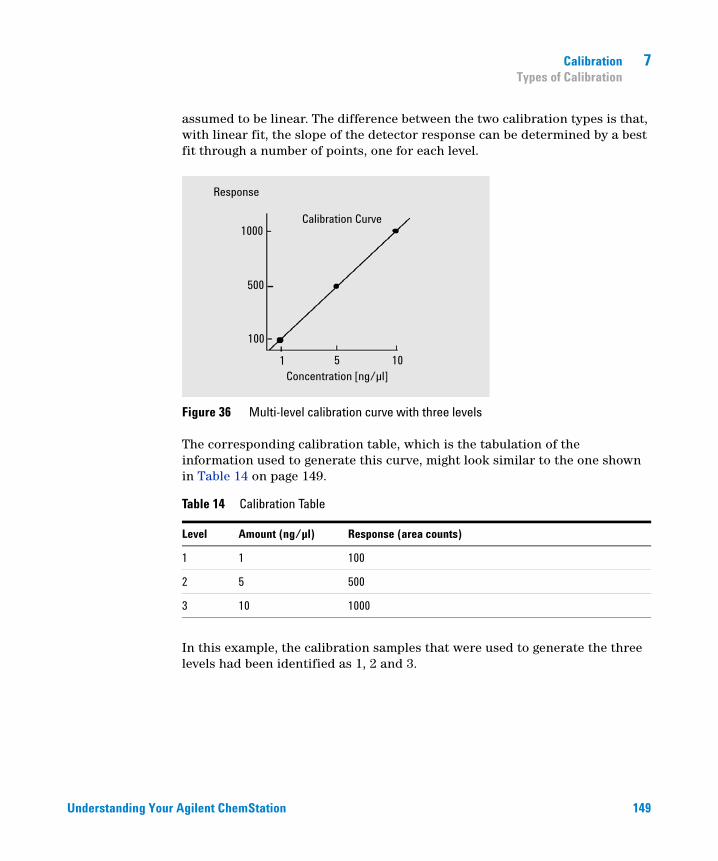
Understanding Your Agilent ChemStation 149
Calibration 7Types of Calibration
assumed to be linear. The difference between the two calibration types is that, with linear fit, the slope of the detector response can be determined by a best fit through a number of points, one for each level.
Figure 36 Multi-level calibration curve with three levels
The corresponding calibration table, which is the tabulation of the information used to generate this curve, might look similar to the one shown in Table 14 on page 149.
In this example, the calibration samples that were used to generate the three levels had been identified as 1, 2 and 3.
Table 14 Calibration Table
Level Amount (ng/µl) Response (area counts)
1 1 100
2 5 500
3 10 1000

150 Understanding Your Agilent ChemStation
7 CalibrationTypes of Calibration
Calibration Ranges
Each multilevel calibration is valid over the range of concentrations used in the calibration samples. Extrapolation of a calibration curve, especially if it is non-linear, is at best an approximation. The valid calibration range for each compound may be defined in the Compound Details dialog box. Each entry for that compound can be expressed as lower and upper limits. If these limits are exceeded, the report is annotated.
Calibration Curve Fits
Various curve-fit calculations are available for use with multilevel calibration.
• Piecewise Linear
• Linear
• Log
• Power
• Exponent
• Quadratic
• Cubic
• Average (Response/Amount)
Non-Linear Fit
In some cases, the detector response to changes in sample concentration is not linear. For these types of analyses, a linear regression calibration method is not appropriate and a multilevel calibration calculation should be used.
Origin Treatment
There are four ways to treat the origin when the response curve is plotted:
• ignore the origin,
• include the origin,
• force the origin, or
• connect the origin.

Understanding Your Agilent ChemStation 151
Calibration 7Types of Calibration
To force the origin to be included in the calibration curve the calibration points are mirrored about the origin from the first quadrant into the third quadrant. Using all points for the regression calculation ensures that the resulting calibration curve passes through the origin. This is also explained in Figure 37 on page 151.
Figure 37 Forcing the origin to be included
For further information about calibration curve fits and origin treatment, see the online help file.
Calibration Point Weighting
When setting up your default calibration curve, you can specify the relative weighting (or importance) of the various calibration points used to generate the curve.
The following weighting options can be selected:

152 Understanding Your Agilent ChemStation
7 CalibrationTypes of Calibration
Quadratic calibration point weightings, for example, can be used to adjust for a spread in calibration points. It makes sure that calibration points closer to the origin, which can normally be measured more accurately, get a higher weight than calibration points further away from the origin, which may be spread.
You should base your decision, which kind of calibration point weighting to use, on your method requirements.
Weight Description
Equal All calibration points have equal weight in the curve.
Linear (Amnt) A calibration point with the amount x has the weighting 1/x normalized to the smallest amount so that the largest weight factor is 1. Normalization is done by multiplying the weight with the smallest amount. For example the weight of a calibration point with the amount x is (1/x) × a where a is the smallest amount of the calibrated compound prepared in the calibration standards.If the origin is included it is assigned the mean of the weightings of the other calibration points.
Linear (Resp) A calibration point with the response y has the weighting 1/y normalized to the smallest response so that the largest weight factor is 1. Normalization is done by multiplying the weight with the smallest response. For example the weight of a calibration point with the amount y is (1/y) × b where b is the response corresponding to the smallest amount of the calibrated compound prepared in the calibration standards. If the origin is included it is assigned the mean of the weightings of the other calibration points.
Quadratic (Amnt) A calibration point with the amount x has the weighting 1/x2normalized to the smallest amount so that the largest weight factor is 1. Normalization is done by multiplying the weight with the smallest amount. For example the weight of a calibration point with the amount x is (1/x²) × a² where a is the smallest amount of the calibrated compound prepared in the calibration standards.
Quadratic (Resp) A calibration point with the response y has the weighting 1/y2 normalized to the smallest response so that the largest weight factor is 1. Normalization is done by multiplying the weight with the smallest response. For example the weight of a calibration point with the response y is (1/y²) × b² where b is the response corresponding to the smallest amount of the calibrated compound prepared in the calibration standards.
# Calibrations A calibration point is weighted according to the number of recalibrations of the point. No normalization is done.

Understanding Your Agilent ChemStation 153
Calibration 7Group Calibration
Group Calibration
Group calibration can be applied for compounds where the individual concentrations are not known but the sum of concentrations for a group of compounds is known. An example are isomers. Complete compound groups are calibrated. The following formulae are used:
Calibration
where:
ConcAB is the concentration of the compound group consisting of compound A and B
ResponseA is the area (or height) of compound A
RFA is the response factor
For compounds within a compound group we assume equal response factors:
Therefore the concentration of a compound within a compound group is calculated as follows:

154 Understanding Your Agilent ChemStation
7 CalibrationPeak Summing
Peak Summing
The peak sum table is provided for certain applications in the petrochemical and pharmaceutical industries that can be performed more effectively with the following features:
• Sum the areas of peaks that lie within a range specified by the user
• Sum the areas of a range of peaks and perform the calculations using a single multiplier
• Sum the areas of all peaks having the same name
The peak sum table is similar to, but distinct from the standard calibration table. Like the calibration table, it is associated with the current method.
NOTE You must create a calibration table for an analysis before you can create the peak sum table.
Understanding Your Agilent ChemStation 155
Calibration 7Recalibration
Recalibration
What is Recalibration?
Recalibration is the process used when you want to update a level on a calibration curve. When you recalibrate you run another sample that contains the same calibration compounds as the original, and most important, the same amount of these compounds. When you run the calibration sample, you obtain updated response factors and retention/migration times. You may also choose to average the response factors over a number of calibration runs so that response factors are weighted equally.
Why Recalibrate?
Most calibrations have a limited lifetime, due to changes in chromatography. Recalibration is necessary to maintain the accuracy of the analysis. For example, assume you have created a calibration table for the compound caffeine which you use whenever you are required to quantify samples containing caffeine. At some point you will need to replace the column/capillary. Although the column/capillary is replaced with exactly the same type, it will not behave in exactly the same way as the previous column/capillary when you first created the calibration table for caffeine. Therefore, to ensure consistency you should recalibrate the levels in the calibration table before using the new column/capillary to analyze samples containing unknown amounts of caffeine. By doing this you are quantifying samples analyzed under the same system conditions.
Manual Recalibration
You can enter peak calibration information manually and normalize the calibration table using the Manual Setup option button in the New Calibration Table dialog box. Typically, a new calibration method is produced by running a calibration standard mixture, creating a calibration table, and entering the amounts of all calibrated peaks to obtain response factors. This approach is

156 Understanding Your Agilent ChemStation
7 CalibrationRecalibration
inefficient for some application, such as found in the petrochemical industry, where the same compounds have been analyzed for many years and the response factors for various compounds and detectors are readily available.
You create the calibration table manually by entering peaks and their response factors into the calibration table, recalibrating the method using a standard that contains at least one response reference peak, and selecting Delta% update.
Recalibrations with Peak Summing
When a recalibration is performed, the retention/migration time ranges in the Peaksum Table of the method will be updated before the actual recalibration is done. Peak Sum recalibrations are performed in this way to ensure the delta is incorporated into the time calculations.
Recalibration Options
You have several ways to update the responses in the calibration table with the new calibration data.
Average
The average from all calibration runs are calculated using the following formula
Floating Average
A weighted average for all calibration runs is calculated. The updated weight is set in the Recalibration Settings dialog box.

Understanding Your Agilent ChemStation 157
Calibration 7Recalibration
Replace
The new response values replace the old values.
Ways to Recalibrate
Recalibration can be done in two ways using the ChemStation software. You can recalibrate interactively or automatically during a sequence of automated analyses. Interactive recalibration is when you directly go through the process of recalibration using the ChemStation software after injecting one or more calibration samples. Recalibration using a sequence is where you specify when the recalibration occurs, but the automation software does the recalibration. For more information refer to “Automatic Recalibration” on page 179.
For information on how to perform recalibration using the software, see the How To part of the help system.
Recalibration of Unidentified Peaks
There are three ways to recalibrate unidentified peaks.
No Recalibration
If a peak in the calibration table cannot be identified in the integration results, the calibration is aborted. If this occurs in a sequence, the sequence is also aborted.
Partial Recalibration
This feature allows the recalibration of only the identified peaks. If peaks are missing, the calibration is not aborted but the report is annotated that peaks are missing.

158 Understanding Your Agilent ChemStation
7 CalibrationRecalibration
Recalibration of all Retention/Migration Times
This feature allows the retention/migration time recalibration of all identified and unidentified peaks. This is done by using the retention/migration times of the identified peaks. There is no update of response factors for unidentified peaks.

159
Understanding Your Agilent ChemStation
Agilent Technologies
8Automation
What is Automation? 161
What is a Sequence/Sequence Template? 162
Preferences - Sequence Tab 163
Sequence Parameters 165
Sequence Table 166
Creating Sequences (Sequences and Sequence Templates) 167
Using the Sequence Table Editor 167
Using the Insert Vial Range Button 167
Using the Append Line Button 167
Using the Custom Fields Button 168
Working with Sequences (Sequences and Sequence Templates) 169
Priority Samples 169
Sequencing with Control Samples 169
Stopping a Sequence 169
Aborting a Sequence 170
Pausing a Sequence 170
Running a Partial Sequence 170
Sequence Log File 172
What Happens When a Sequence is Run? 173
Sequence Data File Structure (Unique Folder Creation ON) 175
Data File Naming in a Sequence 176
Automatic Data File Naming During a Sequence 176
Entering Data File Names Manually 177
Postsequence Operation 178
Not Ready Timeout (LC and CE only) 178
Wait Time (LC and CE only) 178
Automatic Recalibration 179
160 Understanding Your Agilent ChemStation
8 AutomationRecalibration
Specifying Recalibrations 180
Recalibration Parameters in the Sequence Table 180
Types of Sequences 183
Explicit Calibration Sequences 184
Cyclic Single-Level Calibration Sequences 185
Cyclic Multiple-Level Calibration Sequences 186
Method A Analysis Order 187
Method B Analysis Order 188
Explicit and Cyclic Calibrations Together 190
Example 190
SimpReg Analysis Order 191
Cyclic Calibration Sequences with Bracketing 192
Example 192
Bracketed Sequence Operation 193
Example 193
Cyclic Recalibration Sequences with Multiple Vials Containing the Same Dilution of a Standard 196
Cyclic Recalibration Sequence with “Round-Robin” Calibration Vial Usage 196
Cyclic Recalibrations Where Each Calibration Uses a Different Vial 198
Bracketing Sequence that Uses Different Vials for Opening and Closing Bracket 198
This chapter describes the concepts of automation. It explains how to work with sequences in ChemStation, what happens when a sequence is run and how to customize sequences.

Understanding Your Agilent ChemStation 161
Automation 8What is Automation?
What is Automation?
Automation is the unattended analysis of more than one injection.
The sequence part of the ChemStation software allows you to automate acquisition, data evaluation, and report generation.

162 Understanding Your Agilent ChemStation
8 AutomationWhat is a Sequence/Sequence Template?
What is a Sequence/Sequence Template?
A sequence is a series of instructions that automates the analysis of samples.
A sequence can be used to automatically inject each sample, and to acquire and analyze the data according to the method specified for that sample. Each sample vial in a sequence may be analyzed with a different analytical method and, thus, use different sets of chromatographic/electropherographic conditions and evaluation parameters.
ChemStation introduces two data storage modes, to allow you to choose the data storage model that matches your workflow. These modes have influence of the sequence usage:
• Unique Folder Creation ON
• Unique Folder Creation OFF
Unique Folder Creation ON for consistency of sample data uses sequences as “sequence templates” that can be used to run the acquisition multiple times; however, they are not used for reprocessing in Method and Run Control. When the sequence template is run, a sequence data container is created, containing all related files. If the sequence template is reused, a new sequence data container is created for each reuse
Unique Folder Creation OFF stores all data in one directory. The sequence *.s files are not used as sequence templates, so re-executing a sequence again might overwrite present data, if the data directory is not changed from the user.
The available sequence/sequence templates (*.s) are visible in the ChemStation Explorer. For quick and easy navigation, you can add additional sequence/sequence template locations to the ChemStation Explorer selection tree using the Paths tab of the Preferences dialog box.

Understanding Your Agilent ChemStation 163
Automation 8Preferences - Sequence Tab
Preferences - Sequence Tab
On the Sequence tab, the user has the choice of two different data storage models. These modes define how the sequence data are stored in the ChemStation.
Unique Folder Creation ON
In this mode of data storage, there is a robust and permanent link between the raw data and the method. Each data file, whether acquired within a sequence or as a single run, has links to at least two methods: the method that was used to acquire the data, and the one that was used for data analysis.
The sequence data are stored in a sequence data container using a defined sequence container name. You can specify the naming conventions (Name Pattern) for these sequence containers in the Sequence tab of the Preferences dialog box. If no name pattern is specified, a default sequence name pattern is used. The Sequence Tab is used only for data acquisition and therefore is present only for online systems.
The sequence name pattern can contain various sections. The system creates a name for your sequence data container that is determined by the sequence name pattern sections you select. All data files, methods, the sequence logbook, the sequence_name.s file and the sequence_name.b file belonging to this particular sequence are stored in the sequence data container. The sequence data container is created when the sequence is started.
The sequence (.s) files are used as sequence templates, and this concept allows you to run any sequences.s file multiple times without overwriting existing data and without changing the sequence parameters. If neither counter nor time are used in the sequence name pattern, the system introduces a counter automatically to avoid overwriting data. For the second, third and all subsequent sequences using the same sequence template, a counter is added to the sequence container name.

164 Understanding Your Agilent ChemStation
8 AutomationPreferences - Sequence Tab
Unique Folder Creation OFF
In this mode of data storage, the method name is the only link that exists between the data file and the method that was used to acquire and process it. No copies of the method are saved with the sequence or with the data file; if the method is changed, or a new method with that name is created, then the sequence cannot be exactly reproduced.The sequence data files are stored in accordance with the parameters specified in the Data File group of the Sequence Parameters dialog box; the sequence naming facility in the Sequence tab of the Preferences dialog box is disabled in this mode.This mode of data storage is identical to ChemStation revisions prior to B.02.01 and therefore cannot take full advantage of the latest Data reviewing/reprocessing functionalities in the Data Analysis View of the ChemStation.
NOTE Sequence data acquired using the option “Unique folder Creation OFF” need to be reprocessed using the reprocess option in the Method and Run Control view.
NOTE The Add-On solutions G2189BA ChemStation OpenLAB Option and G2181BA ChemStore require the preference mode “Unique Folder Creation ON”. As soon as the Add-On is installed on top of the ChemStation, the option “Unique Folder Creation OFF” is disabled.
Understanding Your Agilent ChemStation 165
Automation 8Sequence Parameters
Sequence Parameters
The Sequence Parameters dialog box contains information common to all sample vials in a sequence. Use this dialog box to:
• select the data directory using the Path combo box, and enter information about the operator name (the operator name entered in the access level dialog box is shown), and
• specify how the sequence processing should be done by choosing particular part of Methods and Run parameters.
For example, you can choose to either:
• execute the run-time checklist,
• do acquisition only, or
• do reprocessing only - for data acquired till ChemStation Rev. B.01.03. - for data acquired with option Unique Folder Creation OFF
If the reprocess option is selected, you have the choice to use the sample data defined when the sample was originally analyzed, or by activating the Use Sequence Table information check box, you can use updated sample data by entering new data in the sequence table:
• specify what happens when the sequence is finished using the shutdown parameters, and
• specify if the barcodes should be used in the sequence and how to handle a barcode mismatch, assuming that a barcode reader is installed on the system.
NOTE Sequence data acquired with ChemStation revisions up to B.01.03 or acquired using the options Unique folder Creation OFF need to be reprocessed using the reprocess option in the Method and Run Control view.
Sequence data acquired with ChemStation revisions B.02.01 and higher need to be reprocessed using the reprocess option in the Data Analysis Navigation table.

166 Understanding Your Agilent ChemStation
8 AutomationSequence Table
Sequence Table
The sequence table determines which methods are used to analyze the sample vials and the order in which the vials are analyzed. This table also contains information about each sample, including the name, quantification parameters, and recalibration parameters.
The injector group box is displayed for instruments that support dual sampling (GC). Selecting Front or Back displays the lines in the sequence table and the currently running status for that injector.
For a description of the columns in this table and how they interact with information stored with the method, see the online help reference.

Understanding Your Agilent ChemStation 167
Automation 8Creating Sequences (Sequences and Sequence Templates)
Creating Sequences (Sequences and Sequence Templates)
Use the sequence table to specify the samples, methods, and vials to run in the sequence. The sequence table lists each sample in the sequence in the order it will be run and contains the necessary vial, method, and calibration information for each sample.
Using the Sequence Table Editor
If you would like to change the view and content of your sequence table, you can open the Sequence Table Editor by clicking the listing symbol in the lower right corner of the Sequence Table. The Sequence Table Editor opens and allows you to specify if a certain column is shown within the Sequence table. In addition the column widths can be defined for each sequence table column. Depending on the installed software packages, additional column fields will be added, for example, “Target Mass” field if an LC/MS is installed, “Study” field for ChemStore Add-On installation.
Using the Insert Vial Range Button
If you have many samples that use the same method, you can quickly enter these samples into the Sequence Table using the Insert Vial Range feature. This feature copies the method name, vial range, number of injections per vial, and if you specify the Sample Amount, ISTD Amount, Multiplier, and Dilution. The system then enters the information for each vial in the range into the sequence table.
Using the Append Line Button
To append a new blank line to the end of the sequence table, select the Append Line button.

168 Understanding Your Agilent ChemStation
8 AutomationCreating Sequences (Sequences and Sequence Templates)
Using the Custom Fields Button
If custom fields have been set up in the method(s) used in the sequence table, select the Custom Fields button in order to edit the custom fields values for each sample (sample related custom fields) or for each compound in the method of a sample (compound related custom fields).
Understanding Your Agilent ChemStation 169
Automation 8Working with Sequences (Sequences and Sequence Templates)
Working with Sequences (Sequences and Sequence Templates)
Sequences (Sequences and Sequence Templates) are accessed and created from the Sequence menu. Sequences may be created and saved in the same way as methods. When you save a sequence, a file is created with a .S extension. When you want to edit or use the sequence again, you access it by, for example, using the Load Sequence item in the Sequence menu.
Priority Samples
A currently running sequence can be paused after the current method is completed. The sequence can be paused to allow the analysis of a priority sample by the same or another method. The sequence can then be resumed, where the sequence continues with the sample at which the sequence was paused.
Sequencing with Control Samples
Control samples can be specified in the Sample Type field of the sequence table. The method used to analyze the control sample must contain a calibration table where control sample limits for one of the compounds are specified. If the control sample limits you specified are exceeded, the sequence is stopped and a message is written into the logbook. If you are using one of the ChemStation report styles, the control sample limits are also printed on the reports generated for these analyses. For more information on how to define a sequence with control samples, see the How To section of the online help system.
Stopping a Sequence
The currently active run will be completed before the sequence stops. A stopped sequence can never be resumed.

170 Understanding Your Agilent ChemStation
8 AutomationWorking with Sequences (Sequences and Sequence Templates)
Aborting a Sequence
The abort function terminates a currently active sequence immediately.
Pausing a Sequence
During a sequence pause, the sequence table file name and the data file name cannot be changed. In the sequence table you can only change sequence lines that have not already been executed or change the vial number in the current sequence line. You can add, delete, and change sequence lines for future analyses.
For example, it may be necessary to edit an active sequence to add a new batch of samples. You can edit the sequence so these vials will be the next sample that the ChemStation will process after the samples in the currently running sequence line.
Running a Partial Sequence
A sequence table that is already set up can be partially executed by selecting Partial Sequence from the Sequence menu. The system displays the Partial Sequence dialog box and allows you to select individual samples from the table for analysis.
A single run is shown on each line of the Partial Sequence dialog box. For each run, the vial, method, data file, and sample name are given. Additionally, encoded information about the sequence table and any calibration samples are shown in the Seq Tbl and Calib:RF:RT columns. See the online help for an explanation of these codes
You can obtain a paper copy of the partial sequence by selecting the Print button.
The following Partial Sequence dialog box results when the SimpReg Method and Sequence Table, shown later in Table 20 on page 190 and Table 21 on page 191, are current. Samples 1, 2, 4, 5, and 8 are marked for processing.
Understanding Your Agilent ChemStation 171
Automation 8Working with Sequences (Sequences and Sequence Templates)
Figure 38 Partial Sequence Dialog Box
Partial Sequence in Preference Mode “Unique Folder Creation ON”
The sequence data are stored in a sequence data container using a defined sequence container name. If you run a partial sequence the system will create a new sequence data container based on the Preference settings, each time a part of that sequence is executed. So it is possible to create e.g. three sequence data container of the same sequence by executing three time a partial sequence based on the one sequence.
Partial Sequence in Preference Mode “Unique Folder Creation OFF”
The sequence data files are stored in accordance with the parameters specified in the Data File group of the Sequence Parameters dialog box. Even if the sequence is executed partially, all data files will be stored in the same subdirectory.

172 Understanding Your Agilent ChemStation
8 AutomationSequence Log File
Sequence Log File
A sequence log file is produced that indicates what has happened during the running of the sequence. It is useful for identifying when errors occurred if the sequence is running unattended or overnight. The name of the logbook file always has the .log extension. The logbook file is located in the directory where the data of the sequence is stored.

Understanding Your Agilent ChemStation 173
Automation 8What Happens When a Sequence is Run?
What Happens When a Sequence is Run?
Starting a Sequence using “Unique Folder Creation ON”
The system creates a sequence data container based on the path definition in the sequence parameters and the sequence preference settings. The sequence template *.s, all methods defined in the sequence table belonging to this particular sequence are copied to the sequence data container. The system continue to work with these files during acquisition. Starting the sequence, the method of the corresponding sequence line is loaded within ChemStation from out these data container.
Starting a Sequence using “Unique Folder Creation OFF”
Starting a sequence, the system is loading the sequence *.s file and based, on the entry in the sequence table the corresponding method of the sequence line is loaded within ChemStation. In contract to the second data storage mode “Unique Folder Creation ON”, no sequence data container is created. Sequence and methods will remain in their master directory.
Further executed steps during sequence execution:
The following steps will be repeated for each executed sequence line:
• If equipped with an autosampler, the ChemStation software first locates the sample in the autosampler according to the number entered in the vial column
• The instrument is loaded with the method parameters.
• The pre-run macro is executed.
• The sample is then injected into the instrument (manually or automatically).
• The method data evaluation is done. Integration, quantification, and reporting, including any user specified macro. In case the mode “Unique Folder Creation ON” is used, the system is storing two additional methods, ACQ.M and DA.M during the run.
• The post-run macro is executed.

174 Understanding Your Agilent ChemStation
8 AutomationWhat Happens When a Sequence is Run?
• During the entire process, the ChemStation tracks the sequence’s progress in real time and produces a sequence log file.
Figure 39 Sequence Status

Understanding Your Agilent ChemStation 175
Automation 8Sequence Data File Structure (Unique Folder Creation ON)
Sequence Data File Structure (Unique Folder Creation ON)
In the ChemStation revision B.02.01 and later, the link between the raw data and the method has been strengthened, as shown in Figure Sequence Data File Structure “Unique Folder Creation ON”.
Figure 40 Sequence Data File Structure

176 Understanding Your Agilent ChemStation
8 AutomationData File Naming in a Sequence
Data File Naming in a Sequence
Data file naming in a sequence can be done in the following ways:
• automatic,
• manual, or
• prefix/counter.
Automatic Data File Naming During a Sequence
Sample Vials
For example 017-0103.D
where:
• The first three digits are the vial number, for example, 017.
• The fourth digit in liquid chromatography and capillary electrophoresis is a separation hyphen (-); in a gas chromatograph, this will be either (F) for front or (B) for back.
• The fifth and sixth digits are the sequence line that defines the method used, for example, 01 for the first sequence line.
• The seventh and eighth digits are the injection number for this vial by the method, for example, 03 for the third injection.
Blank Runs
For example NV--0499.D
where:
• NV stands for no vial.
• - is a separation hyphen.
• 0499 is the 99th blank run of sequence line 4.

Understanding Your Agilent ChemStation 177
Automation 8Data File Naming in a Sequence
Entering Data File Names Manually
One of the columns in the sequence table is named Datafile. When it contains no entry, the data file naming scheme specified (automatic or prefix-counter) is used to create the data file name. If any text is entered into the Datafile column, the ChemStation uses that text as the data file name for the run.
If more than one injection per vial is specified on a line with a manual data file name, the ChemStation automatically truncates characters from the end of the name entered by the user and appends the injection number. This prevents the same data file name from being reused for multiple injections.
Using a Prefix/Counter to Name Data Files
If you use the Prefix/Counter to name data files, the ChemStation generates a name for each analysis. For an instrument that supports dual signal analysis such as the GC, the ChemStation will generate a name for each signal.
The sequence set up allows long filenames for the prefix/counter. The datafile name defined by prefix/counter can have up to fifteen characters plus .d extension, so in total seventeen characters.
Following rules apply to the prefix/counter field:
• the counter itself can have a maximum up to 6 characters
• if a prefix provides less than nine characters for prefix, the counter is automatically extended to 6 digits
• the number given in the counter is the start number being incremented
Table 15
Prefix Counter results in file name
long 000001 long000001
longname 000001 longname000001
testwithalongna 1 testwithalongna1

178 Understanding Your Agilent ChemStation
8 AutomationPostsequence Operation
Postsequence Operation
You can specify what happens after a sequence has finished during normal execution or when the ChemStation encounters an error during sequence operation. For LC operation, this is done by activating the post-sequence Cmd/Macro check box of the Sequence Parameters where you have a choice of:
• Setting the system to a STANDBY state where the pump and lamp are off,
• setting the system to a LAMPOFF state where all lamps are off (LC and CE only),
• Setting the system to a PUMPOFF state where all pumps are off (LC and CE only), or
• Using a default SHUTDOWN macro or modifying SHUTDOWN.MAC to determine specific operation.
For example, you may want to switch off your system after your sequence has completed. Other uses of the shutdown macro could be to set your flow to zero or slowly reduce your flow.
In the Sequence Parameters, you may specify any custom macro to run by including its name in the Post-Sequence Cmd/Macro field and checking the box.
Not Ready Timeout (LC and CE only)
The Not Ready Timeout in the Sequence Parameters is the length of time the system will wait for the instrument to become ready — after this time the system will shut down.
Wait Time (LC and CE only)
Sequence Parameters allows you to specify a wait time which is executed after loading method and before injecting with that method. This can be useful for column/capillary re-equilibration when using new analysis conditions.

Understanding Your Agilent ChemStation 179
Automation 8Automatic Recalibration
Automatic Recalibration
Calibration is often done after a change in operating conditions, for example, after changing a column or capillary. Automatic recalibration is usually done at the start of a sequence of analyses or at regular intervals during a sequence as part of a program to compensate for factors that affect the analytical performance.
There are two ways to specify automatic sequence recalibration:
• explicit calibration sequences, or
• cyclic calibration sequences.
Recalibration using Preference Mode “Unique Folder Creation ON”
While performing a recalibration, the calibration table of the used method is update according the defined method settings. Using the data storage mode “Unique Folder Creation ON”, the recalibrated methods are available within the sequence data container. The calibration table of the sequence method is updated during that process. In addition the DA.M method of the individual data files contains the updated calibration used for result creation.
Recalibration using Preference Mode “Unique Folder Creation OFF”
While performing a recalibration, the calibration table of the used method is update according the defined method settings. Using the data storage mode “Unique Folder Creation OFF”, the calibration table of the master method is update during the recalibration.

180 Understanding Your Agilent ChemStation
8 AutomationSpecifying Recalibrations
Specifying Recalibrations
The recalibration parameters for the sequence are entered directly into the sequence table. These parameters define how the method is recalibrated during a sequence.
Recalibration Parameters in the Sequence Table
The response factor and retention/migration times can be updated in several ways. The calibration level, update response factor and update retention/migration times are instructions used in the data analysis when recalibrating the calibration table.
When Calibration is entered in the SampleType column of the sample table, the following columns become active and can be edited:
• Cal Level
• Update RT
• Update RF
• Interval
The values that can be entered into each of these columns are shown in the table.
Table 16 Recalibration Parameters in Sequence Table
CAL Level Update RT Update RF Interval
Calibration table Level # (1-999)
No update No update Cyclic recalibration interval # (1-999)
Average Average Blank
Replace Replace
Bracket
Delta%

Understanding Your Agilent ChemStation 181
Automation 8Specifying Recalibrations
The table shows the columns in the sequence table that contain the recalibration parameters and the values that can be entered.
No Update
Does not change the response factor or retention/migration time.
Replace
Replaces the previous retention/migration times and the response (areas or heights) with those from the current run only. The response is not changed for any peak that is not found in this recalibration run.
Average
Averages the retention/migration times and responses (areas or heights) for each peak based on the original calibration run and all averaged recalibrations since then. If a peak is missing in one of the recalibrations, the average response of the peak will not suffer.
Bracket
The samples are bracketed by pre-sample and post-sample calibrations. Evaluation is done when the last calibration sample of the closing bracket has been run. The existing calibration data is replaced by the result data of the calibration run of the opening bracket. The closing bracket calibrations are averaged to that calibration table.
Interval
The Interval determines how often a calibration is done during a sequence. Calibration frequency corresponds to the number of sample injections that are done before the next set of calibration injections takes place. At the start of the analysis, a calibration is done and the results (response factors) are entered into the calibration table. These results are then used in subsequent quantitative calculations. After the specified number of injections have been done, another calibration is made and the results are entered into the calibration table overwriting the results of the previous calibration run.

182 Understanding Your Agilent ChemStation
8 AutomationSpecifying Recalibrations
Delta%
The delta% calculation allows you to compare response factors from an analysis with response factors entered manually into a calibration table. The delta% is then applied to all of the calibrated peaks in the table. You can identify several internal standards, and their measured response factors are then used to calculate new response factors for the other peaks. You identify which internal standard is to be used for the delta% calculation for each peak in the calibration table.

Understanding Your Agilent ChemStation 183
Automation 8Types of Sequences
Types of Sequences
The following are types of sequences:
• explicit calibration sequences,
• explicit single-level calibration sequences,
• cyclic multiple-level calibration sequences,
• explicit and cyclic calibrations together in a sequence, and
• cyclic calibration sequences with bracketed calibrations.

184 Understanding Your Agilent ChemStation
8 AutomationExplicit Calibration Sequences
Explicit Calibration Sequences
This type of sequence recalibrates at defined intervals specified by you in the sequence table.
For explicit calibration sequences, the calibration samples are entered in the sequence without an interval entry in the sequence table. A recalibration is done once for each calibration sample entry in the sequence table.

Understanding Your Agilent ChemStation 185
Automation 8Cyclic Single-Level Calibration Sequences
Cyclic Single-Level Calibration Sequences
This type of sequence uses the same vial, that is, the calibration sample at regular intervals in the sequence.
The interval entry in the sequence table determines how the recalibration is done. For example, an interval value of 2 will recalibrate after every two sample vials in the sequence.

186 Understanding Your Agilent ChemStation
8 AutomationCyclic Multiple-Level Calibration Sequences
Cyclic Multiple-Level Calibration Sequences
This type of sequence uses different calibration samples to recalibrate a multiple-level calibrated method.
The following example describes a two-method sequence comprising method A and method B to analyze two groups of samples. Both methods are multiple-level calibration methods that will recalibrate automatically at defined intervals.
For each method the Sequence Table has three entries:
• Two calibration levels:
• Sequence lines 1 and 2 in method A.
• Sequence lines 8 and 9 in method B.
• Five entries for the samples:
• Sequence line 3 through 7 in method A.
• Sequence line 10 through 14 for method B.
The calibrations are specified at regular intervals by the recalibration interval entry in the Sequence Recalibration Table.
• Method A will recalibrate after every two samples.
• Method B will recalibrate after every three samples.
The Sequence Table below is truncated to simplify the example.
Table 17 Sequence Table for Method A and Method B
Line Vial Method Name
Inj/Vial Sample Type
Cal Level
Update RF
Update RT
Interval
1 1 Method A 1 Calibration 1 Average No update
2
2 2 Method A 1 Calibration 2 Average No update
2
3 10 Method A 1
4 11 Method A 1

Understanding Your Agilent ChemStation 187
Automation 8Cyclic Multiple-Level Calibration Sequences
Method A Analysis Order
This section describes the analysis order for Method A which is the first part of the two-method sequence.
5 12 Method A 1
6 13 Method A 1
7 14 Method A 1
8 3 Method B 1 Calibration 1 Average No update
3
9 5 Method B 2 Calibration 2 Average No update
3
10 20 Method B 1
11 21 Method B 1
12 22 Method B 1
13 23 Method B 1
14 24 Method B 1
Table 17 Sequence Table for Method A and Method B
Line Vial Method Name
Inj/Vial Sample Type
Cal Level
Update RF
Update RT
Interval
Table 18 Method A Analysis Order
Inj No. Method Vial Operation
1 Method A 1 Calibration level 1 and report
2 Method A 2 Calibration level 2 and report
3 Method A 10 Sample analysis and report
4 Method A 11 Sample analysis and report
5 Method A 1 Calibration level 1 and report
6 Method A 2 Calibration level 2 and report

188 Understanding Your Agilent ChemStation
8 AutomationCyclic Multiple-Level Calibration Sequences
Method B Analysis Order
This section describes the analysis order for Method B, which is the second part of the two-method sequence.
Method B has the following differences compared with Method A:
• There are two injections per vial for calibration level 2. The Interval entry is set to 3.
7 Method A 12 Sample analysis and report
8 Method A 13 Sample analysis and report
9 Method A 1 Calibration level 1 and report
10 Method A 2 Calibration level 2 and report
11 Method A 14 Sample analysis and report
Table 18 Method A Analysis Order
Table 19 Method B Analysis Order
Inj No. Method Vial Operation
12 Method B 3 Calibration level 1 and report
13 Method B 5 Calibration level 2 and report
14 Method B 5 Calibration level 2 and report
15 Method B 20 Sample analysis and report
16 Method B 21 Sample analysis and report
17 Method B 22 Sample analysis and report
18 Method B 3 Calibration level 1 and report
19 Method B 5 Calibration level 2 and report
20 Method B 5 Calibration level 2 and report
21 Method B 23 Sample analysis and report
22 Method B 24 Sample analysis and report

Understanding Your Agilent ChemStation 189
Automation 8Cyclic Multiple-Level Calibration Sequences
Note that the results shown in Table 18 on page 187and Table 19 on page 188can be obtained by using Partial Sequence to see a preview of the run order after setting up the Sequence Table.

190 Understanding Your Agilent ChemStation
8 AutomationExplicit and Cyclic Calibrations Together
Explicit and Cyclic Calibrations Together
This type of sequence comprises explicit and cyclic calibrations in the same sequence.
This feature allows you to recalibrate the method completely at the beginning of a sequence (explicit recalibration) and then update the calibration (cyclic recalibration) during the sequence.
• Two calibration lines for each calibration level in the Sequence table must be specified. One calibration line is for the explicit recalibration entry and the other for the cyclic recalibration entry.
• The sequence table must have entries for each calibration line and all cyclic recalibration vials must appear before both the explicit recalibration and sample entries.
Example
The sequence table below illustrates a single-level calibrated method called SimpReg. It is truncated to simplify the example.
There are two entries for the single calibration level.
Table 20 Sequence Table for SIMPREG
1 1 SimpReg 1 Calibration 1 Average Average 3
2 1 SimpReg 1 Calibration 1 Replace Replace
3 2 SimpReg 1
4 3 SimpReg 1
5 4 SimpReg 1
6 5 SimpReg 1
7 6 SimpReg 1

Understanding Your Agilent ChemStation 191
Automation 8Explicit and Cyclic Calibrations Together
• The first calibration line is for the same level but averages the calibration parameters. The interval entry specifies that the recalibration is done after every three samples.
• The second entry replaces all the recalibration parameters, that is, a complete recalibration is done. It has no recalibration interval.
Sequence Table
The sequence table comprises seven lines. The first line specifies the cyclic recalibration sample. The second line specifies the explicit recalibration that is done only once at the beginning of the sequence. The third through seventh lines specify the samples to be analyzed.
The order of the entries into the sequence table is very important. All cyclic recalibration vial entries specifying cyclic calibration must appear before the sample entries or any explicit recalibration entries for the method.
SimpReg Analysis Order
This section describes the analysis order for the SimpReg method.
Table 21 SimpReg Analysis Order
Seq Line Inj No. Method Vial Operation
2 1 SimpReg 1 Simple calibration
1 2 SimpReg 1 Regular calibration
3 3 SimpReg 2 Sample analysis
3 4 SimpReg 3 Sample analysis
4 5 SimpReg 4 Sample analysis
5 6 SimpReg 1 Regular calibration
6 7 SimpReg 5 Sample analysis
7 8 SimpReg 6 Sample analysis

192 Understanding Your Agilent ChemStation
8 AutomationCyclic Calibration Sequences with Bracketing
Cyclic Calibration Sequences with Bracketing
In a cyclic calibrated sequence with bracketing, the calibration table used to calculate the unknown quantitative results is generated by averaging the results of the current calibration with those of the previous calibration. This new calibration table is a more accurate representation of the instrument response at the time the sample was analyzed.
Example
Consider the following situation:
• The instrument response is drifting.
• Three injections of an identical two-component mixture are specified.
• Two injections are specified as calibration samples, and one is specified as a sample.
• The first and third are calibration samples.
• The second injection is a sample.
To obtain a precise quantitative result for injection two (the sample), an interpolation must be made between the two calibration samples; see the figure. This process is known as bracketing.

Understanding Your Agilent ChemStation 193
Automation 8Cyclic Calibration Sequences with Bracketing
Figure 41 Bracketing
Bracketed Sequence Operation
• The first calibration vials are analyzed.
• The sample vials are analyzed.
• The next calibration vials are analyzed.
• The calibration table is produced by replacing the existing response factors by new ones and averaging the following calibration runs into a new calibration table.
• The sample vial data files are evaluated, and reports are generated.
• The sequence returns to step 2 if there are more sample vials to be analyzed.
Example
This section describes a sequence bracketing example comprising one method called Brack.M. The Brack.M method is a two-level internal standard method using cyclic calibration.
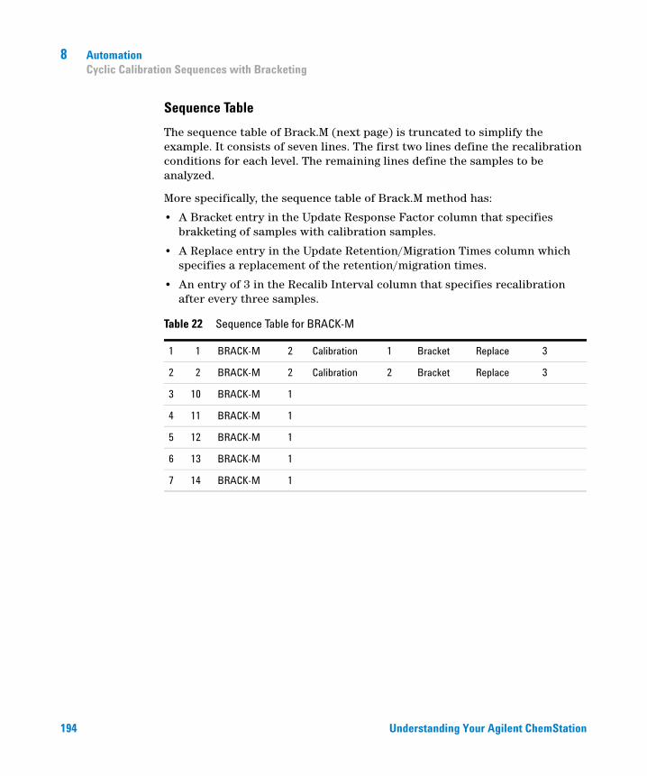
194 Understanding Your Agilent ChemStation
8 AutomationCyclic Calibration Sequences with Bracketing
Sequence Table
The sequence table of Brack.M (next page) is truncated to simplify the example. It consists of seven lines. The first two lines define the recalibration conditions for each level. The remaining lines define the samples to be analyzed.
More specifically, the sequence table of Brack.M method has:
• A Bracket entry in the Update Response Factor column that specifies brakketing of samples with calibration samples.
• A Replace entry in the Update Retention/Migration Times column which specifies a replacement of the retention/migration times.
• An entry of 3 in the Recalib Interval column that specifies recalibration after every three samples.
Table 22 Sequence Table for BRACK-M
1 1 BRACK-M 2 Calibration 1 Bracket Replace 3
2 2 BRACK-M 2 Calibration 2 Bracket Replace 3
3 10 BRACK-M 1
4 11 BRACK-M 1
5 12 BRACK-M 1
6 13 BRACK-M 1
7 14 BRACK-M 1

Understanding Your Agilent ChemStation 195
Automation 8Cyclic Calibration Sequences with Bracketing
Bracketed Sequence Analysis Order

196 Understanding Your Agilent ChemStation
8 AutomationCyclic Recalibration Sequences with Multiple Vials Containing the Same Dilution of a Standard
Cyclic Recalibration Sequences with Multiple Vials Containing the Same Dilution of a Standard
Cyclic Recalibration Sequence with “Round-Robin” Calibration Vial Usage
When running a large sequence that performs cyclic recalibrations, that is, performs an automatic recalibration after a fixed number of sample injections, there is a potential risk of emptying the volume of calibration vial during the course of the sequence. The ChemStation sequence table provides a means of using a series of vials that contain the same dilution of a standard to be used in a round-robin fashion.
With this capability, large sequences can be defined with automatic recalibrations at fixed intervals using multiple calibration vials for each level and each calibration vial would be consumed to the same extent.
By defining an appropriate number of calibration vials, it is even possible to guarantee that each calibration vial is only used once. This is an important requirement in cases where a fresh calibration vial is required for every recalibration, for example, because the analyte evaporates once the septum is punctured or starts degrading after getting in contact with the steel needle. The following section describes how the ChemStation sequence table needs to be set up to fulfill these requirements.
Determine the total number of calibration vials for each level based on the estimated calibrant usage throughout the sequence.
Set up a separate cyclic recalibration line for each calibration vial. Lines defined for the same calibration level must be in adjacent sequence lines and the defined vial positions must be adjacent, too. Choose an identical recalibration interval for all calibration lines. For example, if your sequence should recalibrate after every 6 sample injections, set the recalibration interval to 6.

Understanding Your Agilent ChemStation 197
Automation 8Cyclic Recalibration Sequences with Multiple Vials Containing the Same Dilution of a Standard
The execution order is:
• Vial 1 (Cal1a)
• Vial 5 (Cal2a)
• 6 injections out of vial 10 (Sample10)
• Vial 2 (Cal1b)
• Via 6 (Cal2b)
• 6 injections out of vial 11 (Sample11)
• Vial 3 (Cal1c)
• Vial 7 (Cal2c)
• 6 injections out of vial 12 (Sample12)
• Vial 1 (Cal1a)
• Vial 5 (Cal2a)
• 6 injections out of vial 13 (Sample13)
• Vial 2 (Cal1b)
• Vial 6 (Cal2b)
• etc.
Table 23 Cyclic Recalibration Sequence with 3 Vials Defined for Each Level
Vial No. Sample Name Sample Type Method Name No. of Inj. Lvl Upd RT Upd RF Interval
1 Cal1a Calib MethodA 1 1 Avg Avg 6
2 Cal1b Calib MethodA 1 1 Avg Avg 6
3 Cal1c Calib MethodA 1 1 Avg Avg 6
5 Cal2a Calib MethodA 1 2 Avg Avg 6
6 Cal2b Calib MethodA 1 2 Avg Avg 6
7 Cal2c Calib MethodA 1 2 Avg Avg 6
10 Sample10 Sample MethodA 6
11 Sample11 Sample MethodA 6
12 Sample12 Sample MethodA 6
13 Sample13 Sample MethodA 6
14 Sample14 Sample MethodA 6

198 Understanding Your Agilent ChemStation
8 AutomationCyclic Recalibration Sequences with Multiple Vials Containing the Same Dilution of a Standard
Cyclic Recalibrations Where Each Calibration Uses a Different Vial
To ensure that every calibration vial be injected only once, the sequence must define a sufficient number of different calibration vials, so that the round-robin order described in the previous example is not applied. For example, if the sequence processes 80 sample vials with recalibrations required after every 10 samples, the sequence table must contain 80/10 + 1= 9 calibration lines for each level.
As in the previous example, the calibration lines must be adjacent sequence lines that reference adjacent vial positions.
Bracketing Sequence that Uses Different Vials for Opening and Closing Bracket
The same capability is available for bracketing sequences. By defining the appropriate vial range of calibration vials, a bracketing sequence can be defined so that different calibration vials are used for the opening and closing brackets. In this case, too, calibration lines in the sequence must be adjacent just like the vial positions of the calibration vials.
Whether or not the bracketing calibration vials are used in round-robin mode or for one single injection only simply depends on the total number of calibration vials for each level and the number of recalibrations required by the sequence.
The following example defines 3 sample injections that are bracketed by calibrations. The opening bracket uses a different calibration vial than the closing bracket. Recalibrations are required after every sample injection. so the recalibration interval has to be 1. The number of calibration lines per level is the number of samples plus one.
Table 24 Different Vials Used for Opening and Closing Brackets
Vial No. Sample Name Sample Type Method Name No. of Inj. Lvl Upd RT Upd RF Interval
1 Cal1a Calib MethodA 1 1 Brkt Brkt 1
2 Cal1b Calib MethodA 1 1 Brkt Brkt 1
3 Cal1c Calib MethodA 1 1 Brkt Brkt 1

Understanding Your Agilent ChemStation 199
Automation 8Cyclic Recalibration Sequences with Multiple Vials Containing the Same Dilution of a Standard
The execution order for this sequence is:
• Vial 1 (Cal1a), Opening Bracket 1
• Vial 10 (Sample10)
• Vial 2 (Cal1b), Closing Bracket 1 and Opening Bracket 2
• Vial 11 (Sample11)
• Vial 3 (Cal1c), Closing Bracket 2 and Opening Bracket 3
• Vial 12 (Sample 12)
• Vial 4 (Cal1d), Closing Bracket 3
4 Cal1d Calib MethodA 1 1 Brkt Brkt 1
10 Sample10 Sample MethodA 1
11 Sample11 Sample MethodA 1
12 Sample12 Sample MethodA 1
Table 24 Different Vials Used for Opening and Closing Brackets
Vial No. Sample Name Sample Type Method Name No. of Inj. Lvl Upd RT Upd RF Interval

200 Understanding Your Agilent ChemStation
8 AutomationCyclic Recalibration Sequences with Multiple Vials Containing the Same Dilution of a Standard

201
Understanding Your Agilent ChemStation
Agilent Technologies
9Data Review, Reprocessing and Batch Review
Navigation Table in Data Analysis 202
Navigation Table Configuration 202
Navigation Table Toolbar 203
Data Review Using the Navigation Table 204
Sequence Reprocessing Using the Navigation Table 205
What is Batch Review? 207
Enabling Batch Review Functionality with ChemStation OpenLAB Option Installed 208
Batch Configuration 209
Batch Table 209
Compound Table 209
Batch Report 210
User Interface 210
Review Functions 211
Calibration in Batch Review 211
Batch Reporting 212
Batch History 212
This chapter describes the possibilities to review data and how to reprocess sequence data. In addition it describes the concepts of Batch Review, Batch configuration, review functions, and batch reporting.
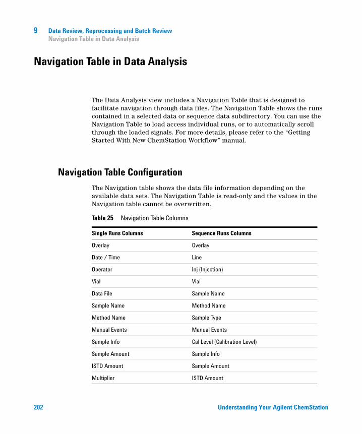
202 Understanding Your Agilent ChemStation
9 Data Review, Reprocessing and Batch ReviewNavigation Table in Data Analysis
Navigation Table in Data Analysis
The Data Analysis view includes a Navigation Table that is designed to facilitate navigation through data files. The Navigation Table shows the runs contained in a selected data or sequence data subdirectory. You can use the Navigation Table to load access individual runs, or to automatically scroll through the loaded signals. For more details, please refer to the “Getting Started With New ChemStation Workflow” manual.
Navigation Table Configuration
The Navigation table shows the data file information depending on the available data sets. The Navigation Table is read-only and the values in the Navigation table cannot be overwritten.
Table 25 Navigation Table Columns
Single Runs Columns Sequence Runs Columns
Overlay Overlay
Date / Time Line
Operator Inj (Injection)
Vial Vial
Data File Sample Name
Sample Name Method Name
Method Name Sample Type
Manual Events Manual Events
Sample Info Cal Level (Calibration Level)
Sample Amount Sample Info
ISTD Amount Sample Amount
Multiplier ISTD Amount

Understanding Your Agilent ChemStation 203
Data Review, Reprocessing and Batch Review 9Navigation Table in Data Analysis
The Navigation table includes standard table configuration features, such as sorting and drag-and-drop options to move columns to different places. It is also possible to select the columns that are displayed in the Navigation Table.
In addition, column-specific grouping is possible, for example, single runs of a particular operator can be displayed by grouping the loaded files by the column “operator”.
The Navigation table offers right mouse click functions to load a signal, overlay a signal, export data, print reports, view the acquisition method parameters etc. Each Navigation Table line can be expanded by clicking the + (plus) sign at the left of the line to configure signal-specific options:
• Signal: Lists the acquired signals and allows you to specify the signals to be loaded. The signal display selection is applied to each run individually.
• General Info: Lists the header details about the run.
• Instrument curves: Allows you to select the instrument data curves to be displayed along with the chromatogram/electropherogram and in the printout.
Navigation Table Toolbar
The Navigation Table includes two toolsets that allow you either to review single run/sequence data, or to reprocess sequence data.
Dilution Multiplier
--- Dilution
--- Data File
Table 25 Navigation Table Columns
Single Runs Columns Sequence Runs Columns

204 Understanding Your Agilent ChemStation
9 Data Review, Reprocessing and Batch ReviewNavigation Table in Data Analysis
Data Review Toolset
The review functionality of the Navigation Table allows you to step automatically or manually through the loaded signals. Depending on the selection specified in the Preferences / Signal/Review Options, the system can automatically integrate the signal and print a report for each file as it is loaded. The method applied to the data file is shown in the top menu.
Sequence Reprocessing Toolset
The sequence reprocessing toolset is available only when a sequence acquired with ChemStation B.02.01 or higher is loaded that was acquired with Unique Folder Creation switched on. It is possible to start, stop and pause the reprocessing of the sequence. In addition, the toolbar gives access to the following dialog boxes in order to change parameter for reprocessing sequences and printing:
• Sequence Table (copy of the original *.s template, located in the sequence data container)
• Sequence Parameters dialog box
• Sequence Output dialog box
• Sequence Summary Parameters dialog box
• Extended Statistic Parameters dialog box
• Save Current Sequence
• Print Current Sequence
Data Review Using the Navigation Table
Depending on your required workflow, you can review data in one of three ways:
1 Review your sequence data using the individual method of each data file (sequence data B.02.01or higher): Use the option Individual Method from Data File (DA.M) in the Preferences / Signal/Review Options to have the system load the individual data analysis method (DA.M) stored with the data file before loading sequence data. As each line in the Navigation Table is accessed during the data review process, the linked DA.M for the selected data file is loaded and used for reviewing and generating the report. The method name
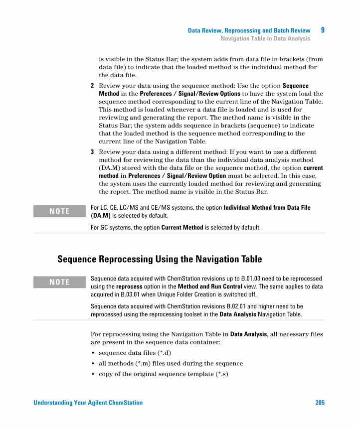
Understanding Your Agilent ChemStation 205
Data Review, Reprocessing and Batch Review 9Navigation Table in Data Analysis
is visible in the Status Bar; the system adds from data file in brackets (from data file) to indicate that the loaded method is the individual method for the data file.
2 Review your data using the sequence method: Use the option Sequence Method in the Preferences / Signal/Review Options to have the system load the sequence method corresponding to the current line of the Navigation Table. This method is loaded whenever a data file is loaded and is used for reviewing and generating the report. The method name is visible in the Status Bar; the system adds sequence in brackets (sequence) to indicate that the loaded method is the sequence method corresponding to the current line of the Navigation Table.
3 Review your data using a different method: If you want to use a different method for reviewing the data than the individual data analysis method (DA.M) stored with the data file or the sequence method, the option current method in Preferences / Signal/Review Option must be selected. In this case, the system uses the currently loaded method for reviewing and generating the report. The method name is visible in the Status Bar.
Sequence Reprocessing Using the Navigation Table
For reprocessing using the Navigation Table in Data Analysis, all necessary files are present in the sequence data container:
• sequence data files (*.d)
• all methods (*.m) files used during the sequence
• copy of the original sequence template (*.s)
NOTE For LC, CE, LC/MS and CE/MS systems, the option Individual Method from Data File (DA.M) is selected by default.
For GC systems, the option Current Method is selected by default.
NOTE Sequence data acquired with ChemStation revisions up to B.01.03 need to be reprocessed using the reprocess option in the Method and Run Control view. The same applies to data acquired in B.03.01 when Unique Folder Creation is switched off.
Sequence data acquired with ChemStation revisions B.02.01 and higher need to be reprocessed using the reprocessing toolset in the Data Analysis Navigation Table.

206 Understanding Your Agilent ChemStation
9 Data Review, Reprocessing and Batch ReviewNavigation Table in Data Analysis
• sequence-related batch (*.b) file
• sequence-related logbook (*.log) file
During reprocessing, the individual methods DA.M for the data files are updated as well as the batch file (*.b) file.
With the Data Analysis reprocessing functions, it is possible to modify the sequence template (*.s) in the data container in order to change the multiplier, dilution etc., or to use a different method for reprocessing. By default, the Data Analysis reprocessing sequence parameter parts of method to run is set to Reprocessing only, and the option Use Sequence Table Information is checked. These predefined default values enable you to change the parameters in the sequence template and run a reprocess without editing the Data Analysis sequence parameters again.
If you have not explicitly changed the method in the sequence template, the system uses the sequence methods stored in the sequence data container to reprocess the sequence. These methods are the original methods used during data acquisition. Note that, even if the option load DA method from data file in Preferences / Signal/Review Options is selected, the system uses the sequence container method for reprocessing, not the DA.M of the individual data files.
If particular method parameters need to be changed (for example, specify to print to a *.xls file), the methods in the sequence container need to be modified and saved. This general change is then applied to all data files during reprocessing.
If you now want to use the updated sequence container method for further data acquisition, you need to copy this method from the sequence data container to one of the defined method paths. The new/updated method is then available in the ChemStation Explorer in the method view as a master method.

Understanding Your Agilent ChemStation 207
Data Review, Reprocessing and Batch Review 9What is Batch Review?
What is Batch Review?
Batch review is a capability within data analysis designed to help an analyst perform a “first-pass” review of the results of a sequence or a selection of runs quickly and easily. It will save time especially when reprocessing large numbers of samples. Whenever a sequence is run, a batch file (with a .b extension) is automatically generated and placed in the data directory along with the data files. This batch file contains pointers to the data files in the batch review itself. Upon loading a batch, the analyst need only select the method to use for the batch, and then individually select the desired data files to analyze in the batch. One can check the calibration accuracy, instrument performance and individual integrations before approving the results. Any chromatogram specific integration parameters which are modified can be stored with the data file for data traceability. This interactive environment provides complete access to all other data analysis capabilities, such as peak purity, library searching, etc., as well.
Batch review uses the same data analysis registers (ChromReg and ChromRes) as the standard data analysis and should therefore not be used in an online session that is currently performing analyses.

208 Understanding Your Agilent ChemStation
9 Data Review, Reprocessing and Batch ReviewEnabling Batch Review Functionality with ChemStation OpenLAB Option Installed
Enabling Batch Review Functionality with ChemStation OpenLAB Option Installed
When ChemStation OpenLAB Option is installed, the Batch Review functionality is not available by default. In order to use Batch Review, this functionality has to be enabled by an entry in the [PCS] section of the ChemStation.ini file. The file is located in the windows directory c:\ WINDOWS.
[PCS] _BatchReview=1
The default entry, _BatchReview=0, turns off the functionality.

Understanding Your Agilent ChemStation 209
Data Review, Reprocessing and Batch Review 9Batch Configuration
Batch Configuration
A batch is a user-selected series of data files that is processed using a user-defined method. All data files in the batch are processed using the same method. The processing steps carried out each time a new sample is loaded for review can be selected (integration, identification/quantitation, reporting).
All calibration runs in the batch are used to produce a single calibration table, using averaged response factors, which is then used for quantification.
Batch Table
Runs are displayed in a user-configurable batch table:
• the number and content of the table’s columns can be specified;
• the runs can be sorted by
• run index (the order in which the runs were acquired) independent of any other criteria,
• sample type (control samples first, then calibration samples, then normal samples) then by run index within each sample type,
• method (if more than one method was used to acquire the runs) then by run index within each method;
• samples, calibration samples and control samples can be displayed in the table or hidden.
Each selected run occupies a line in the batch table. You can exclude a run in the batch table (e.g. from calibration) by changing its sample type to Removed.
Compound Table
The compound results are displayed in a user-configurable compounds table, but contents of the compounds table depends on the type of samples in the batch table:

210 Understanding Your Agilent ChemStation
9 Data Review, Reprocessing and Batch ReviewBatch Configuration
• the compound list contains all compounds found in the method that was loaded for batch review.
• if calibration samples only are displayed in the batch table (samples and control samples are hidden), the compound table shows additional columns for calibration-related information (expected amount, relative error and absolute error).
• if control runs only are displayed in the batch table (samples and calibration samples are hidden), the compound table shows additional columns for any defined control limits.
For columns containing compound-specific information, you can include the name of the compound in the table title by adding %s to the column specification.
Batch Report
The batch report contains two tables that are generally analogous to the batch table and the compound table; these tables are also user-configurable.
For columns containing compound-specific information, you can include the name of the compound in the table title by adding %s to the column specification. Multi-line headers are allowed; you insert the character ‘|’ at the point where you want the line to break.
User Interface
Batch review provides a choice of two user interfaces:
• the standard interface includes a button bar, with buttons mirroring most of the Batch menu items, together with the batch table and compound table;
• a minimal interface provides a button bar similar to the standard interface, but replaces the batch table and compound table with a combo box that contains only the information specified for the batch table. The minimal interface button bar does not contain batch table-related or compound table-related buttons.

Understanding Your Agilent ChemStation 211
Data Review, Reprocessing and Batch Review 9Review Functions
Review Functions
Data files can be displayed in one of two ways:
• manually, by selecting a run to display from the table,
• automatically, with a predefined interval between each data file. During automatic display, only those sample types displayed in the table are displayed; the runs are displayed in the order in which they appear in the table. The automatic review can be paused and later resumed, or stopped.
The standard functions provided by the ChemStation are available with batch review. This includes calibration, manual manipulation of chromatograms, for example by smoothing or manual integration. Any changes made to a data file can be marked and saved with the batch file. Chromatograms that have been reviewed are marked with an asterisk in the batch table. You can also discard changes made to either the current chromatogram only, or all changes to all chromatograms in the batch.
When a run is loaded, the selected processing options are performed; if the run has already been processed and the changes saved, the processed run is loaded. This is a faster process than loading the unprocessed run, because no processing needs to be done.
Calibration in Batch Review
Calibration in batch review works independently from the recalibration settings in the sequence table. The first step in batch calibration always replaces both response and retention time entries in the calibration table. For the following calibration standards, both response and retention time values are averaged.

212 Understanding Your Agilent ChemStation
9 Data Review, Reprocessing and Batch ReviewBatch Reporting
Batch Reporting
The user-configurable “Batch Table” on page 209, can be printed directly on the printer, displayed on the screen or printed to a file with a user-specified prefix in one of the following formats:
• UNICODE text file with the extension .TXT
• Data Interchange Format with the extension .DIF
• Comma-Separated Values format with the extension .CSV
• Microsoft Excel format with the extension .XLS.
The reporting options also give the possibility of sorting the samples (by Run Index, Sample Type or Method) independent of the sort method in the batch table. The sort priorities are as for the “Batch Table” on page 209.
Batch History
Batch review maintains a log of all actions relating to the current batch. Any action that changes the batch (for example changing the displayed chromatogram, changing the sample type, loading and saving the batch) adds a line to the batch history with a date and time stamp, the current operator name and a description of the event.
You can also add your own comments to the batch history. Existing batch history entries cannot be edited, and the history list cannot be accessed except through the Batch History menu item.
213
Understanding Your Agilent ChemStation
Agilent Technologies
10Using the ChemStation Reports
What is a Report? 214
Reporting Results 215
Uncalibrated Reports 215
Calibrated Reports 215
External Standard Report 215
Internal Standard Report 216
Control Charts Report 216
Quantitative Results 217
Reporting Custom Field Values 219
Report Styles 220
Adding a Customized Report to Report Styles 222
Other Report Style Parameters 223
Summed Peaks Table 223
Report Layout for Uncalibrated Peaks 223
Report Destination 224
Report File Formats 224
Sequence Summary Reporting 226
Overview 226
Setting up a Sequence Summary Report 226
This chapter describes what a report is. It gives details on reporting results, quantitative results, report styles, report destination, and sequence summary reporting.

214 Understanding Your Agilent ChemStation
10 Using the ChemStation ReportsWhat is a Report?
What is a Report?
A report can comprise quantitative and qualitative information of the sample you analyze. The report can be a hardcopy printout, a display on the screen or an electronic file. The report can include details of the peaks detected during the run and plots of the signals that were acquired.

Understanding Your Agilent ChemStation 215
Using the ChemStation Reports 10Reporting Results
Reporting Results
Two types of reports are available:
• an uncalibrated report which does not correct for detector response, and
• a calibrated report that shows results corrected for the difference in the detector response to various components of the sample.
Uncalibrated Reports
The uncalibrated reports include the Area% and Height% reports. These reports are mainly used in the preparation of calibrated reports. They may be of value as a final report if the amounts of compound required to produce a unit area or height response for the compounds of interest are similar.
Calibrated Reports
Calibrated reports correct for the difference in the detector response to the reported compounds. One or more calibration samples containing known amounts of the reported compounds must be run under the same conditions used for the unknown sample. The integration data from these calibration sample(s) are used to prepare a calibration table. This is a list of retention/migration times, amounts and responses which is used in the generation of the report. The calibrated reports are based on two calibration procedures called external standard and internal standard.
External Standard Report
The ESTD report lists the results with the units of your choice or with each compound as a percentage of all the compounds present. The external standard procedure requires that the relative injected volume of both the

216 Understanding Your Agilent ChemStation
10 Using the ChemStation ReportsReporting Results
calibration and unknown samples must be known accurately. The reliability of the external standard report is limited by the reproducibility of the injection and any other factors that might change from sample to sample.
Internal Standard Report
The limitations of the external standard procedure can be overcome by using the internal standard approach. An accurately known amount (not necessarily the same amount) of the internal standard is added to both the calibration sample(s) and unknown sample. The response of each compound of interest is divided by the response of the internal standard to give a response ratio. The calibration curves are a plot of this response ratio versus the amount ratio and this information is used in the calculation of the reported results. In this way inadvertent errors in injection volume or slight changes in the chromatographic/electropherographic system that affect all compounds similarly are cancelled out. The ISTD report lists the results with units of your choice.
Control Charts Report
The Control Charts Report tracks a single result from multiple runs for a specific calibrated compound. The Control Chart feature is installed after the ChemStation is operational. Methods that use this feature pass the tracked result to a Microsoft Excel work sheet after each run. Excel is then used to print the report.

Understanding Your Agilent ChemStation 217
Using the ChemStation Reports 10Quantitative Results
Quantitative Results
The report type is identified by the name of the calculation method used to prepare it, for example, an ISTD report. Each type is briefly described below. The calculations for each report are given in “Quantitative Results” on page 217.
Area% provides the simplest report and requires no calibration data since no correction is made for the difference in detector response of sample components. The Area% report is particularly useful in developing a calibration table for use with the other report options. This report is suitable for analyses in which the difference in detector response of the components is not significant.
Height% gives a report similar to the Area% report except that peak height is used for the calculations instead of peak area.
Norm% gives a report in which each component is reported as a percentage of all the components present. The peaks are corrected for detector response before calculation of the percentage of each.
ESTD produces a report of the actual amount of each substance in whatever units you choose. Amounts are calculated using a previously established calibration table. The use of an external standard requires that the injected volume of the calibration mixture be known.
ESTD% produces a report of the relative amount of each substance as a percentage of the injected sample. Amounts are calculated using a previously established calibration table. The use of an external standard requires that the injected volume of the calibration mixture be known.
ISTD produces a report of the actual amount of each substance. Amounts are calculated using a previously established calibration curve. The use of an internal standard in both the sample and the calibration mixture eliminates the need to know and control the volume of the sample injected. This also corrects for any variation in instrument performance between runs.
218 Understanding Your Agilent ChemStation
10 Using the ChemStation ReportsQuantitative Results
ISTD% produces a report of the relative amount of each substance as a percentage of the injected sample. The use of an internal standard in both the sample and the calibration mixture eliminates the need to know and control the volume of sample injected. This also corrects for any variation in instrument performance between runs.

Understanding Your Agilent ChemStation 219
Using the ChemStation Reports 10Reporting Custom Field Values
Reporting Custom Field Values
The values of the custom fields attached to a certain sample according to its acquisition method can be added to the report. Sample custom fields are listed at the end of the report header that contains the general sample information. Compound custom fields appear at the end of the report.

220 Understanding Your Agilent ChemStation
10 Using the ChemStation ReportsReport Styles
Report Styles
The following report styles are available:
You choose to add a signal to any of the report styles by checking the appropriate box in the Specify Report dialog box.
• None - No text will be reported. The chromatogram will be reported only if the Add Chromatogram Output option is selected.
• Short - Comprises quantitative text results of all integrated signals which are setup in the Signal Details dialog box (LC only) or the Signal dialog box (GC only). The peak width in the short report is calculated with the more complex formula used by the integrator: PW = 0.3(IPRight - IPLeft) + 0.7(Area/Height) where IPRight and IPLeft are the inflection points.
• Detail - Comprises header, quantitative results, and calibration curves. The header is stored in a file called RPTHEAD.TXT in the method directory. You can change the header using a text editor to include a method specific text.
• Header + Short - Comprises file header and quantitative text results. The header is stored in a file called RPTHEAD.TXT in the method directory. You can change the header using a text editor to include a method specific text.
• GLP + Short - Comprises header, sample information, instrument conditions, logbook, signal, and quantitative results. The header is stored in a file called RPTHEAD.TXT in the method directory. You can change the header using a text editor to include a method specific text.
• GLP + Detail - Comprises header, sample information, instrument conditions, logbook, signal, quantitative results, and calibration curves. The header is stored in a file called RPTHEAD.TXT in the method directory. You can change the header using a text editor to include a method specific text.
• Full - Comprises header, sample information, instrument conditions, logbook, signals, and quantitative results. The header is stored in a file called RPTHEAD.TXT in the method directory. You can change the header using a text editor to include a method specific text.
• Performance - Produces a report according to the limits specified in the Edit Performance Limits dialog box of the System Suitability menu.

Understanding Your Agilent ChemStation 221
Using the ChemStation Reports 10Report Styles
For uncalibrated methods, the report parameters include the peak number, retention/migration time, peak area, peak height, signal description, true half-height peak-width (see also “True Peak Width Wx [min]” on page 246), symmetry, k’, efficiency (plates) and resolution for each peak.
For calibrated methods, the report parameters include the peak number, retention/migration time, compound name, amount, signal description, true half-height peak-width, symmetry, k’, efficiency (plates) and resolution for each peak.
The half-height peak calculation is not the same as the more complex peak width formula used by the integrator. The values of efficiency and resolution are based on this calculated peak width. The report header consists of all method relevant information, including instrument, column/capillary, sample, and acquisition parameters. The signal is also plotted.
• Performance + Noise- Combines the Performance report style with the noise calculations for the noise ranges defined in the Edit Noise Range dialog box of the System Suitability menu. In addition, the noise, given as six times the standard deviation, as peak-to-peak, and as ASTM noise.The drift and wander is also determined.
• Performance + Extended- Produces an extended report with all the parameters from the peak performance calculations and individual plots of each peak. The plots include the baseline, the tangents, and the peak widths at defined heights. This report type includes only calibrated peaks.
In addition to the parameters printed for the Performance report style, more Peak Performance Parameters are determined: the peak start and end peak times, skew, excess, peak width, USP tailing factor, time interval between data points, number of data points, statistical moments, plates, plates per meter, selectivity and resolution of each peak are printed. The peak width, plates, plates per meter, selectivity, and resolution are calculated by the true half height, 5 sigma, tangent and tailing methods (please refer to “Performance Test Definitions” on page 244 for details).
The report header consists of all method relevant information such as instrument, column/capillary, sample and acquisition parameters and a plot of the signal. For a complete list of the peak performance parameter algorithms see “Performance Test Definitions” on page 244.
The spectral report styles (Short + Spectrum, Detail + Spectrum, Performance + Library Search) are described in Understanding Your Spectra Module.
222 Understanding Your Agilent ChemStation
10 Using the ChemStation ReportsReport Styles
Adding a Customized Report to Report Styles
You can add a custom report template that you have created in the Report Layout view of the ChemStation to the list of available report styles.
NOTE All reports apart from the performance reports list the peakwidths calculated with a more complex formula by the integrator (for details on the peakWidth calculation please refer to “Peak Width” on page 80).

Understanding Your Agilent ChemStation 223
Using the ChemStation Reports 10Other Report Style Parameters
Other Report Style Parameters
Summed Peaks Table
The peak sum table is provided for certain applications in the petrochemical and pharmaceutical industries that can be performed more effectively with the following features:
• Sum the areas of peaks that lie within a range specified by the user
• Sum the areas of a range of peaks and perform the calculations using a single multiplier
• Sum the areas of all peaks having the same name
When the report is generated, the ChemStation uses the peak sum table to produce a peak sum report that is printed after the standard report calculations with the exception of Norm% which is replaced by the peak sum report.
Report Layout for Uncalibrated Peaks
To change the report layout for uncalibrated peaks, choose one of the following in the Specify Report dialog box.
• Separately to report the uncalibrated peaks in a separate table if sorting by retention/migration time is selected, or separate tables if sorting by signal is selected.
• With Calibrated Peaks to report the uncalibrated peaks together with the calibrated peaks.
• Do Not Report to suppress the reporting of uncalibrated peaks.

224 Understanding Your Agilent ChemStation
10 Using the ChemStation ReportsReport Destination
Report Destination
The report can be sent to either:
• Screen
The report (including text and graphics) is displayed on the screen in the report preview window from which it can be printed.
• Printer
The report comprising text and graphics is printed on the currently selected printer.
• File
The report is saved to a file. If the data is saved to a file it is possible to reprocess the data with another program, for example, Microsoft Windows EXCEL.
Report File Formats
A report can be saved in different formats. Each format has a specific extension. It is possible to select more than one format for a report.
.TXT The report text is printed as a UNICODE text file.
.EMF Each report graphic (signal or calibration curve) is saved in a Microsoft Windows metafile (WMF). Several .WMF files for one report are possible. The generated file format adheres to the Microsoft standard metafile format as defined in the Windows software development documentation. These files are compatible with the Aldus Placeable Metafile (APM) format used by a number of proprietary software packages.
.DIF The tabular report data is saved in Data Interchange Format (DIF). This format is accepted by spreadsheet programs, for example, Microsoft Windows EXCEL. Independent from the report style selected, only the information contained in the report style Short will be saved.

Understanding Your Agilent ChemStation 225
Using the ChemStation Reports 10Report Destination
.CSV The report is in Comma Separated Values (CSV) format. This is a very simple format for tabular data that is accepted by many spreadsheet programs and databases. Independent from the report style selected, only the information contained in the report style “Short” will be saved.
There can be several .DIF and .CSV files for a single report. For each report block, the first file, for example, REPORT00.CSV, contains the report header information. Subsequent files contain the tabular results.
If the results are sorted by retention/migration time, only one file is required for the complete table, for example, REPORT01.CSV.
If the results are sorted by signal, a separate table is required for each signal. In this case, the files are named Report01.CSV through ReportNN.CSV, where NN is the number of the signal.
.XLS The report is exported to a Microsoft Excel spreadsheet in (XLS) format. The data generally requires additional processing.
.PDF The report is printed to a .pdf file. The ChemStation setup installs a PDF printer, called "PDF-XChange 4.0". This Printer will only be visible in the Start Menu/Settings/Printers and Faxes until the computer is restarted. When ChemStation is started, another temporary printer is created called "ChemStation PDF" based on the PDF-XChange printer. While any ChemStation session is running, ChemStation PDF will be listed in the Start Menu/Setting/Printers and Faxes. The option Unique pdf file name allows to store the .pdf reports independent of the reports, with file names <sequence_container_name>_<data_file_name>.pdf

226 Understanding Your Agilent ChemStation
10 Using the ChemStation ReportsSequence Summary Reporting
Sequence Summary Reporting
Overview
The ChemStation can print a variety of standard reports for individual sample analyses. Sequence summary reporting is an additional way of reporting, that allows you to calculate and report parameters across a number of different analyses. It is useful, for example, to test the stability of an instrument or the robustness of a new method.
A sequence summary report may include:
• a title page,
• instrument configuration, including the revision numbers of the instrument and details of the analytical column/capillary being used,
• sequence table listings which describe what the automated sequence of analyses should have done,
• logbook descriptions of what the sequence actually did and any unexpected events which occurred during the sequence,
• method listings,
• individual reports on each sample,
• statistics on the analyses based on selected criteria—statistics are calculated only for calibrated compounds, and
• a table of contents with page number references to the detailed sections of the report.
Setting up a Sequence Summary Report
When setting up a sequence summary report, you can select any combination of the following nine categories by activating the appropriate check boxes and, where appropriate, selecting a report style from the template selections. Each template specifies the contents and layout of that particular section of the whole sequence summary report.
You can choose one of the following sequence summary report styles:
Understanding Your Agilent ChemStation 227
Using the ChemStation Reports 10Sequence Summary Reporting
One Page Header
The GLP template prints GLP in large letters as a title page for the following report. It also includes the date and a place for a signature.
Configuration
Select Configuration if you want to include the instrument configuration and analytical column/capillary specifications in the report.
Sequence Table
Select Sequence Table to include a list of the samples, sample quantification parameters and method names in the report. This list shows what the system should have run.
Logbook
Select Logbook for a listing of the analyses the system ran, including instrument conditions and any unusual events that occurred while the samples were being analyzed.
Methods
Select Methods to list all the analytical methods used in the series of automated analyses.
Analysis Reports
Select Analysis Reports to get individual analysis reports according to the report style set up for the method.
Individual analytical reports may be printed after each analysis according to the report style specified for the method in question, in addition to the report sections specified in Sequence Summary Reporting. See "Sequence Output" below.
SUILabel Type = Application > Statistics for Calibrated and Sample Runs
Selecting the Statistics cal. runs will produce statistical trend analyses for calibration samples. Selecting the Statistics sample runs will produce statistical trend analyses for sample (unknown) analyses. Both selections have Standard Statistic and Extended Statistic template styles. Extended Statistics
228 Understanding Your Agilent ChemStation
10 Using the ChemStation ReportsSequence Summary Reporting
prints the statistical trends of the analyses as graphs, whereas the Standard Statistics selection prints only text. The selections that you make in the Items and Limits for Extended Statistics dialog box are used only when you choose the Extended Statistic option(s) in the Sequence Summary Parameters dialog box.
If you choose the Standard Statistic option(s) in the Sequence Summary Parameters dialog box, then the statistics reported are:
• retention/migration time,
• area,
• height,
• amount,
• peak width (based on the report style, see “Report Styles” on page 220)
• symmetry.
The statistic calculation does not distinguish between different calibration levels in a sequence that uses multilevel calibration methods. This means that the concentration-dependent items, for example, Area, Height, Amount (see the dialog box for Items and Limits for Extended Statistics) are all taken together, regardless of the calibration level. The Statistics for Calibration Runs values are therefore not useful for multilevel calibration methods in sequences.
Summary
The Summary selection will print an overview of the series of samples analyzed and the methods used. If the Summary choice is selected together with other Sequence Summary selections, page numbers referring to the other parts of the sequence summary report are included. Two Summary styles are available:
The Sample Summary tabulates details of the sample analyses run in the sequence, with some sample information such as the sample name, data file name, method and vial number.
The Compound Summary tabulates the sample analyses with basic quantification results for each calibrated compound, or each peak, depending on the type of report specified in the method.
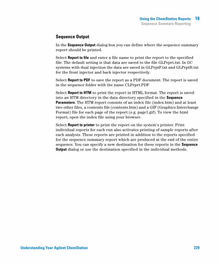
Understanding Your Agilent ChemStation 229
Using the ChemStation Reports 10Sequence Summary Reporting
Sequence Output
In the Sequence Output dialog box you can define where the sequence summary report should be printed.
Select Report to file and enter a file name to print the report to the specified file. The default setting is that data are saved to the file GLPrprt.txt. In GC systems with dual injection the data are saved in GLPrptF.txt and GLPrptB.txt for the front injector and back injector respectively.
Select Report to PDF to save the report as a PDF document. The report is saved in the sequence folder with the name CLPrprt.PDF
Select Report to HTM to print the report in HTML format. The report is saved into an HTM directory in the data directory specified in the Sequence Parameters. The HTM report consists of an index file (index.htm) and at least two other files, a contents file (contents.htm) and a GIF (Graphics Interchange Format) file for each page of the report (e.g. page1.gif). To view the html report, open the index file using your browser.
Select Report to printer to print the report on the system’s printer. Print individual reports for each run also activates printing of sample reports after each analysis. These reports are printed in addition to the reports specified for the sequence summary report which are produced at the end of the entire sequence. You can specify a new destination for these reports in the Sequence Output dialog or use the destination specified in the individual methods.

230 Understanding Your Agilent ChemStation
10 Using the ChemStation ReportsSequence Summary Reporting

231
Understanding Your Agilent ChemStation
Agilent Technologies
11Evaluating System Suitability
Noise Determination 235
Noise Calculation Using Six Times the Standard Deviation 235
Noise Calculation Using the Peak-to-Peak Formula 236
Noise Calculation by the ASTM Method 237
Signal-to-noise calculation 239
Drift and Wander 239
Calculation of Peak Symmetry 240
System Suitability Formulae and Calculations 242
General Definitions 243
Void Volume 243
Retention Time of Unretained Compound t (m) [min] 243
Performance Test Definitions 244
Statistical Moments 244
Statistical Moments, Skew and Excess 245
True Peak Width Wx [min] 246
Capacity Factor (USP), Capacity Ratio (ASTM) k' 246
USP Tailing Factor (USP) t 246
Number of Theoretical Plates per Column (USP, ASTM) n 247
Number of Theoretical Plates per Meter N [1/m] 248
Relative Retention (USP, ASTM), Selectivity Alpha 248
Resolution (USP, ASTM) R 249
Definitions for Reproducibility 250
Sample Mean M 250
Sample Standard Deviation S 250
Relative Standard Deviation RSD[%] (USP) 251
Standard Deviation of the Mean SM 251
Confidence Interval CI 252
Regression Analysis 253

232 Understanding Your Agilent ChemStation
11 Evaluating System SuitabilitySequence Summary Reporting
Regression Coefficient 254
Standard Deviation (S) 254
Internally Stored Double Precision Number Access 255
This chapter describes what the ChemStation can do to evaluate the performance of both the analytical instrument before it is used for sample analysis and the analytical method before it is used routinely and to check the performance of analysis systems before, and during, routine analysis.
Evaluating the performance of both the analytical instrument before it is used for sample analysis and the analytical method before it is used routinely is good analytical practice. It is also a good idea to check the performance of analysis systems before, and during, routine analysis. The ChemStation software provides the tools to do these three types of tests automatically. An instrument test can include the detector sensitivity, the precision of peak retention/migration times and the precision of peak areas. A method test can include precision of retention/migration times and amounts, the selectivity, and the robustness of the method to day-to-day variance in operation. A system test can include precision of amounts, resolution between two specific peaks and peak tailing.
Laboratories which have to comply with:
• good Laboratory Practice regulations (GLP),
• good Manufacturing Practice regulations (GMP) and Current Good Manufacturing Practice regulations (cGMP), and
• good Automated Laboratory Practice (GALP).
Laboratories are advised to perform these tests and to document the results thoroughly. Laboratories which are part of a quality control system, for example, to comply with ISO9000 certification, will have to demonstrate the proper performance of their instruments.
The ChemStation collates results from several runs and evaluates them statistically in the sequence summary report.
The tests are documented in a format which is generally accepted by regulatory authorities and independent auditors. Statistics include:
• peak retention/migration time,
• peak area,
• amount,

Understanding Your Agilent ChemStation 233
Evaluating System Suitability 11Sequence Summary Reporting
• peak height,
• peak width at half height,
• peak symmetry,
• peak tailing,
• capacity factor (k´),
• plate numbers,
• resolution between peaks,
• selectivity relative to preceding peak,
• skew, and
• excess.
The mean value, the standard deviation, the relative standard deviation and the confidence interval are calculated. You can set limits for either standard deviation, the relative standard deviation or the confidence interval for each of these parameters. Should the values exceed your limits, the report is flagged to draw your attention to them.
The quality of the analytical data can be supported by keeping records of the actual conditions at the time the measurements were made. The ChemStation’s logbook records instrument conditions before and after a run. This information is stored with the data and reported with sample data. Instrument performance curves are recorded during the entire analysis as signals, and stored in the data file. If supported by the instrument these records, overlaid on the chromatogram, can be recalled on demand, for example, during an audit.
Baseline noise and drift can be measured automatically. A minimum detectable level can be calculated from peak height data for each calibrated compound in the method.
Finally, instrument configuration, instrument serial numbers, column/capillary identification, and your own comments can be included in each report printed.
Extended performance results are calculated only for compounds calibrated for in the method, ensuring characterization by retention/migration times and compound names.

234 Understanding Your Agilent ChemStation
11 Evaluating System SuitabilitySequence Summary Reporting
A typical system performance test report contains the following performance results:
• instrument details,
• column/capillary details,
• analytical method,
• sample information,
• acquisition information,
• signal description and baseline noise determination, and
• signal labeled with either retention/migration times, or compound names.
In addition, the following information is generated for each calibrated compound in the chromatogram:
• retention/migration time,
• k´,
• symmetry,
• peak width,
• plate number,
• resolution,
• signal-to-noise ratio, and
• compound name.
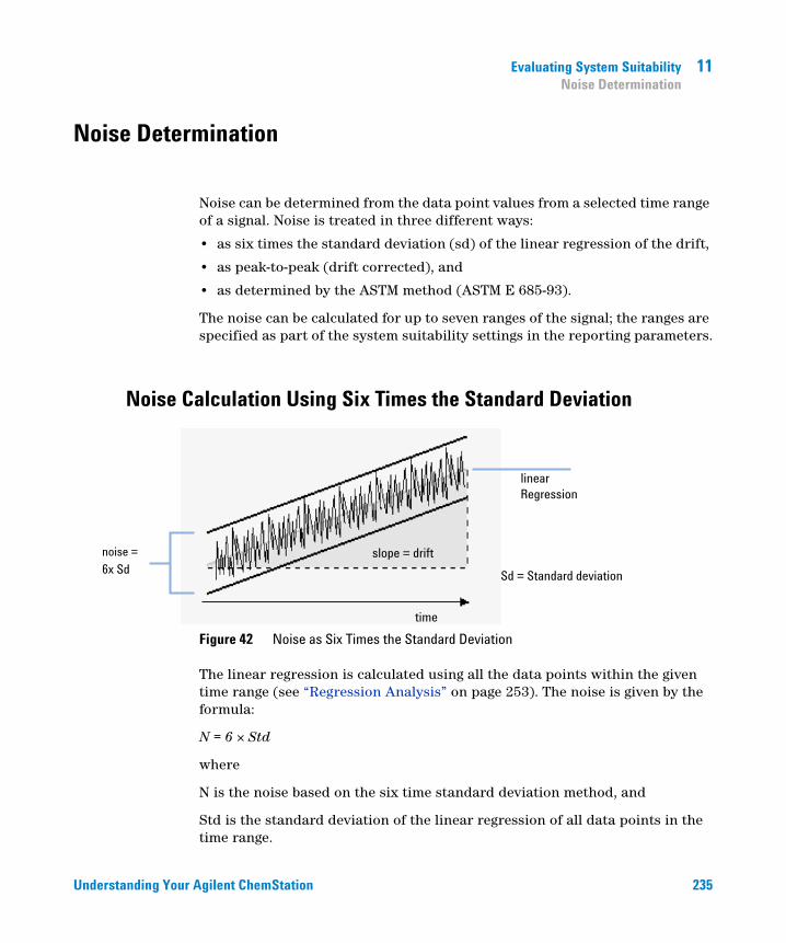
Understanding Your Agilent ChemStation 235
Evaluating System Suitability 11Noise Determination
Noise Determination
Noise can be determined from the data point values from a selected time range of a signal. Noise is treated in three different ways:
• as six times the standard deviation (sd) of the linear regression of the drift,
• as peak-to-peak (drift corrected), and
• as determined by the ASTM method (ASTM E 685-93).
The noise can be calculated for up to seven ranges of the signal; the ranges are specified as part of the system suitability settings in the reporting parameters.
Noise Calculation Using Six Times the Standard Deviation
Figure 42 Noise as Six Times the Standard Deviation
The linear regression is calculated using all the data points within the given time range (see “Regression Analysis” on page 253). The noise is given by the formula:
N = 6 × Std
where
N is the noise based on the six time standard deviation method, and
Std is the standard deviation of the linear regression of all data points in the time range.

236 Understanding Your Agilent ChemStation
11 Evaluating System SuitabilityNoise Determination
Noise Calculation Using the Peak-to-Peak Formula
Figure 43 Noise as Maximum Peak to Minimum Peak (Distance)
The drift is first calculated by determining the linear regression using all the data points in the time range (see “Regression Analysis” on page 253). The linear regression line is subtracted from all data points within the time range to give the drift-corrected signal. The peak-to-peak noise is then calculated using the formula:
N = Imax - Imin
where
N is the peak-to-peak noise,
Imax is the highest (maximum) intensity peak and
Imin is the lowest (minimum) intensity peak in the time range.
{

Understanding Your Agilent ChemStation 237
Evaluating System Suitability 11Noise Determination
Noise Calculation by the ASTM Method
Figure 44 Noise Determined by the ASTM Method
ASTM noise determination (ASTM E 685-93) is based on the standard practice for testing variable-wavelength photometric detectors used in liquid chromatography, as defined by the American Society for Testing and Materials. Based on the size of the time range, three different types of noise can be distinguished. Noise determination is based on peak-to-peak measurement within defined time ranges.
Cycle Time, t
Long-term noise, the maximum amplitude for all random variations of the detector signal of frequencies between 6 and 60 cycles per hour. Long-term noise is determined when the selected time range exceeds one hour. The time range for each cycle (dt) is set to 10 minutes which will give at least six cycles within the selected time range.
Short-term noise, the maximum amplitude for all random variations of the detector signal of a frequency greater than one cycle per minute. Short-term noise is determined for a selected time range between 10 and 60 minutes. The time range for each cycle (dt) is set to one minute which will give at least 10 cycles within the selected time range.
Very-short-term noise (not part of ASTM E 685-93), this term is introduced to describe the maximum amplitude for all random variations of the detector signal of a frequency greater than one cycle per 0.1 minute.

238 Understanding Your Agilent ChemStation
11 Evaluating System SuitabilityNoise Determination
Very-short-term noise is determined for a selected time range between 1 and 10 minutes. The time range for each cycle (dt) is set to 0.1 minute which will give at least 10 cycles within the selected time range.
Determination of the Number of Cycles, n
where t is the cycle time and ttot is the total time over which the noise is calculated.
Calculation of Peak-to-Peak Noise in Each Cycle
The drift is first calculated by determining the linear regression using all the data points in the time range (see “Regression Analysis” on page 253). The linear regression line is subtracted from all data points within the time range to give the drift-corrected signal. The peak-to-peak noise is then calculated using the formula:
where N is the peak-to-peak noise, Imax is the highest (maximum) intensity peak and Imin is the lowest (minimum) intensity peak in the time range.
Calculation of ASTM Noise
where NASTM is the noise based on the ASTM method.
An ASTM noise determination is not done if the selected time range is below one minute. Depending on the range, if the selected time range is greater than, or equal to one minute, noise is determined using one of the ASTM methods previously described. At least seven data points per cycle are used in the calculation. The cycles in the automated noise determination are overlapped by 10 %.

Understanding Your Agilent ChemStation 239
Evaluating System Suitability 11Noise Determination
Signal-to-noise calculation
For the signal-to-noise calculation, the ChemStation uses the six times the standard deviation (sd) of the linear regression of the drift to calculate the noise. The range closest to the peak is selected from the ranges as specified in the system suitability settings. The signal-to-noise is calculated using the formula:
The signal-to-noise is calculated for each peak in the signal. If the ChemStation cannot find a noise value, the signal-to-noise is reported as “-”.
Drift and Wander
Drift is given as the slope of the linear regression, see Figure Noise as Six Times the Standard Deviation, and wander is determined as the peak-to-peak noise of the mid-data values in the ASTM noise cycles, see Noise Determined by the ASTM Method.

240 Understanding Your Agilent ChemStation
11 Evaluating System SuitabilityCalculation of Peak Symmetry
Calculation of Peak Symmetry
The ChemStation does not determine the asymmetry ratio of a peak, usually done by comparing the peak half-widths at 10% of the peak height, or 5% as recommended by the FDA.
Peak symmetry is calculated as a pseudomoment by the integrator using the following moment equations:
If no inflection points are found, or only one inflection point is reported, then the peak symmetry is calculated as follows:

Understanding Your Agilent ChemStation 241
Evaluating System Suitability 11Calculation of Peak Symmetry
Figure 45 Calculation of the Peak Symmetry Factor
where:
ai = area of slice
ti = time of slice
Hf = height of front inflection point
Hr = height of rear inflection point
H = height at apex

242 Understanding Your Agilent ChemStation
11 Evaluating System SuitabilitySystem Suitability Formulae and Calculations
System Suitability Formulae and Calculations
The ChemStation uses the following formulae to obtain the results for the various System Suitability tests. The results are reported using the Performance, Performance + Noise and Performance + Extended report styles.
When ASTM or USP is specified for a given definition, then the definition conforms to those given in the corresponding reference. However, the symbols used here may not be the same as those used in the reference.
The two references used in this context are:
• ASTM: Section E 682 – 93, Annual Book of ASTM Standards, Vol.14.01
• USP: The United States Pharmacopeia, XX. Revision, pp. 943 - 946

Understanding Your Agilent ChemStation 243
Evaluating System Suitability 11General Definitions
General Definitions
Void Volume
where:
d = diameter of column [cm]
π = constant, ratio of circumference to diameter of a circle
l = length of column [cm]
f = fraction of column volume that is not taken up by stationary phase but available for mobile phase; default value for f = 0.68 (for Hypersil)
Retention Time of Unretained Compound t (m) [min]
(Also referred to as dead time or void time)
where:
F = flow rate of LC [ml/min]

244 Understanding Your Agilent ChemStation
11 Evaluating System SuitabilityPerformance Test Definitions
Performance Test Definitions
Statistical Moments
where:
N = Number of area slices
Ai = Value of area slice indexed by i
dt = Time interval between adjacent area slices
t0 = Time of first area slice
= Sum of starting index 1 to final index N for discrete observations

Understanding Your Agilent ChemStation 245
Evaluating System Suitability 11Performance Test Definitions
Statistical Moments, Skew and Excess
Statistical moments are calculated as an alternative to describe asymmetric peak shapes. There is a infinite number of peak moments, but only the first
five are used in connection with chromatographic peaks. These are called 0th
Moment, 1st Moment, … 4th Moment.
The 0th Moment represents the peak area.
The 1st Moment is the mean retention time, or retention time measured at the center of gravity of the peak. It is different from the chromatographic retention time measured at peak maximum unless the peak is symmetrical.
The 2nd Moment is the peak variance which is a measure of lateral spreading. It is the sum of the variance contributed by different parts of the instrument system.
The 3rd Moment describes the vertical symmetry or skew. It is a measure of the departure of the peak shape from the Gaussian standard. The skew given additionally in the Performance & Extended report is its dimensionless form. A symmetrically peak has a skew of zero. Tailing peaks have positive skew and their 1. Moment is greater than the retention time. Fronting peaks have negative skew and their 1. Moment is less than the retention time.
The 4th Moment or excess is a measure of the compression or stretching of the peak along a vertical axis, and how this compares to a Gaussian standard for which the 4. Moment is zero. It can be visualized by moving in or pulling apart the sides of a Gaussian peak while maintaining constant area. If the peak is compressed or squashed down in comparison, its excess is negative. If it is taller, its excess is positive. Also the excess is given in the Performance & Extended report in its dimensionless form.

246 Understanding Your Agilent ChemStation
11 Evaluating System SuitabilityPerformance Test Definitions
True Peak Width Wx [min]
Capacity Factor (USP), Capacity Ratio (ASTM) k'
where:
TR = retention time of peak [min]
T0 = void time [min]
USP Tailing Factor (USP) t
where:
tw = distance in min between peak front and TR, measured at 5% of the peak height
W5.0 = peak width at 5% of peak height [min]
WB base width, 4 sigma, obtained by intersecting tangents through the inflection points with the baseline (tangent peak width)
W4.4 width at 4.4% of height (5 sigma width)
W5.0 width at 5% of height (tailing peak width), used for USP tailing factor
W50.0 width at 50% of height (true half-height peak width or 2.35 sigma).

Understanding Your Agilent ChemStation 247
Evaluating System Suitability 11Performance Test Definitions
Figure 46 Performance Parameters
Number of Theoretical Plates per Column (USP, ASTM) n
Tangent method (USP, ASTM):
where:
WB = base width [min]
Half-width method (ASTM):
where:
W50 = peak width at half-height [min]

248 Understanding Your Agilent ChemStation
11 Evaluating System SuitabilityPerformance Test Definitions
5 Sigma method:
where:
W4.4 = peak width at 4.4% of peak height [min]
Variance method:
where:
Mx = x th statistical moment (see also “Statistical Moments” on page 244)
Number of Theoretical Plates per Meter N [1/m]
where:
n = number of theoretical plates
l = length of column [cm]
Relative Retention (USP, ASTM), Selectivity Alpha
(Pertaining to peaks a and b, TR of peak a < TR of peak b)
where:
k'(x) = capacity factor for peak x

Understanding Your Agilent ChemStation 249
Evaluating System Suitability 11Performance Test Definitions
Resolution (USP, ASTM) R
(Pertaining to peaks a and b, TR of peak a < TR of peak b; TR in min)
Tangent method (USP, ASTM):
5 Sigma method:
Half-width method (Resolution used in Performance Report):
Statistical method:
where:
M1(x) = mean retention time for peak x (1st Statistical Moment) [min]
WB(x) = base width for peak x [min]
W4.4(x) = width at 4.4% height for peak x [min]
W50(x) = width at 50% height for peak x [min]
WS(x) = width derived from statistical moments = for peak x [min] (see also “Statistical Moments” on page 244)

250 Understanding Your Agilent ChemStation
11 Evaluating System SuitabilityDefinitions for Reproducibility
Definitions for Reproducibility
For the statistical review of analytical data in terms of reproducibility the sequence is considered as a small random sample taken out of an infinite number of possible experimental results. To accomplish a complete set of results, an unlimited amount of sample material as well as time would be required. Strictly statistical data does only apply to a complete self-contained set or population of data. Therefore a prerequisite for such a treatment is that the selected sample can be assumed as representative for all data.
Sample Mean M
The mean value M of a random sample consisting of N measurements is calculated from this limited set of N single observed values Xi indexed with a consecutive counter i according to the formula:
where:
N = number of discrete observations
Xi = value of discrete observations indexed by i
Sample Standard Deviation S
Consider a random sample of size N. The sample standard deviation S for the selected finite sample taken out of the large population of data is determined by

Understanding Your Agilent ChemStation 251
Evaluating System Suitability 11Definitions for Reproducibility
The sample standard deviation S differs in two points from the standard deviation s for the whole population:
• instead of the real mean value only the sample mean value M is used and
• division by N-1 instead of N.
Relative Standard Deviation RSD[%] (USP)
The relative standard deviation is defined as
Standard Deviation of the Mean SM
Let M be the sample mean and S the sample [or (N-1)] standard deviation. The standard deviation SM of the sample mean M is determined by
This can be further illustrated by an example:
While the retention time of a certain compound may deviate slightly from the calculated mean value during one sequence, the data from another sequence may differ much more due to e.g. ambient temperature changes, degradation of the column material over time etc. To determine this deviation the standard deviation of the sample mean SM can be calculated according to the above formula.

252 Understanding Your Agilent ChemStation
11 Evaluating System SuitabilityDefinitions for Reproducibility
Confidence Interval CI
The confidence interval is calculated to give information on how good the estimation of a mean value is, when applying it to the whole population and not only to a sample.
The 100 × (1 - α) % confidence interval for the overall mean is given by
where:
percentage point of the t distribution table at a risk probability of α)
For the extended statistics in the sequence summary report the 95% confidence interval may be used (α = 0.05).
The t distribution (or ‘student distribution’) must be used for small sample volumes. In case of large sample volumes the results for the t distribution and the normal (gaussian) distribution do not differ any more. Therefore in case of 30 or more samples the normal distribution can be used instead (it would be very difficult to calculate the t-distribution for large numbers, the normal distribution is the best approximation of it).
95% Confidence Interval for 6 samples:
1 - α = 0.95
N = 6
The correct value for t has to be taken from the t distribution table for 5 (N-1) degrees of freedom and for the value α/2, being 0.025. This would give the following calculation formula for CI:

Understanding Your Agilent ChemStation 253
Evaluating System Suitability 11Definitions for Reproducibility
Regression Analysis
Let
N = number of discrete observations
Xi = independent variable, ith observation
Yi = dependent variable, ith observation
Linear function:
Coefficients:
where:

254 Understanding Your Agilent ChemStation
11 Evaluating System SuitabilityDefinitions for Reproducibility
Regression Coefficient
where:
Standard Deviation (S)

Understanding Your Agilent ChemStation 255
Evaluating System Suitability 11Internally Stored Double Precision Number Access
Internally Stored Double Precision Number Access
For validation purposes, it might become necessary to manually recalculate the ChemStation results such as calibration curves, correlation coefficients, theoretical plates, etc. When doing so the number format used in the ChemStation has to be taken into account.
For all numbers stored internally within the ChemStation, the “C” data type DOUBLE is used. This means that 14 significant digits are stored for each number. The implementation of this data type adheres to the Microsoft implementation of the IEEE standard for “C” data type and the associated rounding rules (see Microsoft documents Q42980, Q145889 and Q125056).
Due to the non-limited number of parameters that might be used for the calculation of the calibration table, it is not possible to calculate the exact error possibly introduced by the propagation and accumulation of rounding errors. Thorough testing with different calibration curve constructions however has shown that the accuracy of up to 10 digits can be guaranteed. Whereas the area, height and retention time repeatability of a chromatographic analysis usually has 3 significant digits, 10 significant digits within the calculations is sufficient. For this reason, the calibration, and other tables, display a maximum of 10 significant digits.
If an external (manual) calculation for validation is required, it is recommended that all digits used for the internal calculations are utilized. Using the displayed and/or rounded data for the external calculations might give results differing from the ChemStation due to rounding errors.
The following paragraph describes how to access all internally stored digits for numbers typically required for manual calculations. In all cases, a data file must be loaded and reported with the appropriate report style prior to execution of the listed command. All commands are entered on the ChemStation command line which may be enabled from the view menu. The information in file “C:\CHEM32\TEMP.TXT” may be viewed using NOTEPAD or a suitable TEXT editor.
Raw Peak Information:
• Retention Time

256 Understanding Your Agilent ChemStation
11 Evaluating System SuitabilityInternally Stored Double Precision Number Access
• Area
• Height
• Width (integrator)
• Symmetry
• Peak Start Time
• Peak End Time
Use Command Line Entry:
DUMPTABLE CHROMREG, INTRESULTS,”C:\CHEM32\1\TEMP\INTRES.TXT”
Processed Peak Information:
• Measured Retention Time
• Expected Retention Time
• Area
• Height
• Width (integrator)
• Symmetry
• Half Width - Half Peak Height (Performance & Extended Performance)
• Tailing Factor (Performance & Extended Performance)
• Selectivity (Performance & Extended Performance)
• K` (Extended Performance)
• Tangent Peak Width (Extended Performance)
• Skew (Extended Performance)
• Theoretical Plates - Half Width (Performance & Extended Performance)
• Theoretical Plates - Tangent (Extended Performance)
• Theoretical Plates – 5-Sigma (Extended Performance)
• Theoretical Plates - Statistical (Extended Performance)
• Resolution - Half Width (Performance & Extended Performance)
• Resolution - Tangent (Extended Performance)
• Resolution – 5-Sigma (Extended Performance)
• Resolution - Statistical (Extended Performance)

Understanding Your Agilent ChemStation 257
Evaluating System Suitability 11Internally Stored Double Precision Number Access
Use Command Line Entry:
DUMPTABLE CHROMRES, PEAK,”C:\CHEM32\1\TEMP\PEAK.TXT”
Processed Compound Information:
• Calculated Amount
Use Command Line Entry:
DUMPTABLE CHROMRES, COMPOUND,”C:\CHEM32\1\TEMP\COMPOUND.TXT”
Calibration Table Information:
• Level Number
• Amount
• Area
• Height
Use Command Line Entry:
DUMPTABLE _DAMETHOD, CALPOINT,”C:\CHEM32\1\TEMP\CALIB.TXT”
Linear Regression Information:
• Y-Intercept (CurveParm1)
• Slope (CurveParm2)
• Correlation Coefficient
Use Command Line Entry:
DUMPTABLE _DAMETHOD, PEAK,”C:\CHEM32\1\TEMP\REGRESS.TXT”

258 Understanding Your Agilent ChemStation
11 Evaluating System SuitabilityInternally Stored Double Precision Number Access

259
Understanding Your Agilent ChemStation
Agilent Technologies
12System Verification
Verification and Diagnosis Views 260
System Verification 260
The GLPsave Register 263
DAD Test Function 265
Review DAD Test Function 265
This chapter describes the verification function and the GLP verification features of the ChemStation.

260 Understanding Your Agilent ChemStation
12 System VerificationVerification and Diagnosis Views
Verification and Diagnosis Views
If supported by the configured instrument, for example, the Agilent 1100/1200 Series modules for LC, the ChemStation comprises two additional views to perform instrument verification and diagnosis tasks. For more information, see the online help system.
System Verification
System verification is a key component in the routine use of an analytical instrument in a regulated laboratory. The GLP verification features of the ChemStation are designed to help you to prove that the software, or a relevant components of the software, are performing correctly, or were performing correctly at the time of a particular analysis.
The ChemStation verification function enables you to verify the correct operation of your ChemStation software. You can do this by reprocessing data files according to specific methods, and comparing the results with a pre-defined standard. The verification function is particularly important to prove the integrity of the integration and quantification results.
You can use the standard verification test, or define your own tests using your own method and data files to check the algorithmic software combinations used by your analysis methods. The verification test is a protected file and cannot be changed or deleted.
The Verification item in the Data Analysis view allows you to choose any of the following options:
• run a verification test in the database,
• define a new verification test and add it to the database, and
• delete a verification test from the database.
The How To section of the online help system describes how to perform these tasks. When running a ChemStation verification test, you can choose whether to run the entire test, or select a combination of parts.

Understanding Your Agilent ChemStation 261
System Verification 12Verification and Diagnosis Views
Verification test results are saved in binary format to the default subdirectory: c:\CHEM32\1\Verify, together with the method and data files. The Verify subdirectory is at the same level as the sequence, methods and data subdirectories. You can send the results to a printer or to a file. The test results, including a combined verification test result, are rated as either pass or fail.
The following verification test components are available:
Digital Electronics (Agilent 1100/1200 Series DAD only)
A test chromatogram is stored in the diode-array detector. This chromatogram is sent to the ChemStation after it has gone through the same preprocessing steps as normal raw data from the photodiodes. The resulting data are compared to original result data stored in the ChemStation for this test chromatogram. If there is a mismatch the test fails. This test ensures that the DAD electronics which do the data preprocessing are still functioning correctly. As a stored test chromatogram is used, the lamp or the diode array are not part of this test. They can be checked with the “DAD Test Function” on page 265.
Peak Integration
The data file is integrated again using the original method. The results are compared to the original integration results stored in verification register. If they do not match, the test fails.
Compound Quantification
The compounds in the data file are quantified again. The results are compared to the original quantification results stored in the verification register. If they do not match, the test fails.
Report Printing
The original report is printed again.
The following page shows an example of a successfully completed verification test.
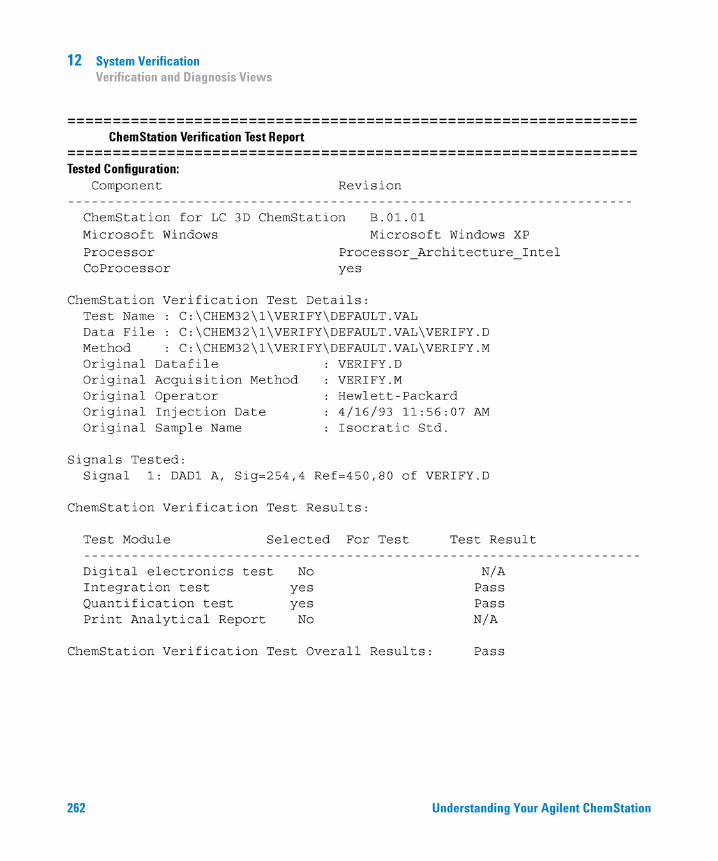
262 Understanding Your Agilent ChemStation
12 System VerificationVerification and Diagnosis Views
Understanding Your Agilent ChemStation 263
System Verification 12The GLPsave Register
The GLPsave Register
The GLPsave register is saved at the end of each analysis when selected in the run time checklist. It contains the following information:
• signals,
• logbook,
• integration results table,
• quantification results table,
• instrument performance data, and
• data analysis method.
This register is a complete protected record, generated at the time of analysis. You can recall it at any time in the future as proof of your analytical methods.
The GLPsave Register option in the Data Analysis view enables you to review the GLPsave register file at any time. The file is protected by a checksum and is encoded into binary to ensure it is not changed.
In the dialog box used to select the GLPsave register for review, you can choose your review options from the following:
• load original method,
• load original signals,
• load instrument performance data,
• print original method,
• print original integration results,
• print original quantification results, and
• generate original report from the original method and signals.
You can use the GLP review function to show that chromatographic data are original, prove the quality of the analysis from the instrument performance data, and demonstrate the authenticity of the data interpretation.
For example, you can:

264 Understanding Your Agilent ChemStation
12 System VerificationThe GLPsave Register
• reload and reprint the data analysis part of the method used at the time of the sample analysis to prove that the data evaluation, presented as the results of the analysis has not been modified in any way, and
• review without recalculating, the integration and quantification results to prove the authenticity of the report.
Understanding Your Agilent ChemStation 265
System Verification 12DAD Test Function
DAD Test Function
Detector tests can be used as a step in the routine system validation of an analytical instrument in a regulated laboratory.
The DAD test assesses the performance of your diode array detector. When you select the DAD test from the Instrument menu (for LC3D and CE only) it checks the instrument for intensity and wavelength calibration. When you press Save the test results are automatically saved to the DADTest database, a register file called DADTest.Reg located in the default instrument directory.
Review DAD Test Function
The Review DAD Test function in the data analysis View menu enables you to review the DADTest.Reg file at any time. The file is protected by a checksum, and is encoded into binary to ensure that it is not changed.
You can select any of the following parts of the DAD test for review:
Show HolmiumSpectra
Plots all Holmium spectra listed in the DAD Test review table. The active spectrum is tagged.
Show IntensitySpectra
Plots all intensity spectra listed in the DAD Test review table. The active spectrum is tagged.
Save as NewDatabase
If you change the lamp in your DAD you can reset the DADTest by deleting any unwanted test results from the table and then using the Save as New Database function.
Show SelectedSpectra
Displays only spectra you selected in the table.
Show IntensityGraph
You can plot an intensity graph to give an indication of the life of the lamp in your diode array detector. The graph provides a function of maximum lamp intensity against time.

266 Understanding Your Agilent ChemStation
Index
Index
Aabort
sequence 170
absoluteresponse factor 116retention time 130retention time 132
accuracyanalysis 157
amount limits 131
amount limits 148
analog signal 60
analysisaccuracy 157
apex 73
area reject 105
area%calculation 118report 217
ASTM noise determination 237
automaticbatch review 211library search 54recalibration 179shutdown 178
automation 27, 159what is? 161
Bbaseline allocation 89
baseline tracking 74
baseline allocation 75
baseline construction 89
baseline penetration 91
batch reviewautomatic 211history 212manual 211user interface 210
batch reportingoutput formats 212
batch tableconfiguration 209removed sample type 209reporting 212
batchcompound table 209configuration 209report 210
blankruns 176
bracketedcalibration 181
bracketingcyclic calibration 192
bunching 82
Ccalculation
calibrated 119ESTD 120ISTD 123norm% 122peak symmetry 240quantification 115uncalibrated 118
calibration curvemultiple-level 148types 147
calibration table 128what is? 143
calibration curvecalibration point weighting 151description of 144fits 151force through zero (origin) 151single-level 147what is? 144
calibration"Round-Robin" 196bracketed 181bracketing operation 193compound 142curve fits 151curve 144cyclic single-level 185cyclic multiple-level 186explicit 184frequency 181level 142multiple-level 148point 142ranges 150sample 142settings 126
capacity factor 246
capacity ratio 246
cardinal points 76
ChemStationcustomization 26general description 38general description 11
CI 252
compound table 209

Understanding Your Agilent ChemStation 267
Index
compound 142
confidence interval 252
configuration 15
control chart reports 26
control limits 210
corrected retention time 130, 134
correction factors 116
curvecalibration 144fits 151
customizationdata analysis 55
customizedreports 25
cyclic recalibration 196
cyclic calibrationbracketing 192
DDa.M 56
data acquisition 19
data analysiscustomized 55integration 21quantification 22reporting 22
data evaluation modules 12
data files 209
data acquisitionwhat is? 60
data analysisspecialized reporting 23
dead time 243
delta% 182
derivative 74, 81
destinationreport 224
detector response 215
detector response 147
digital signal 60
dilution factor 116
dilution factor 120
directorymethod 51structure 34
documentation 32
Eend time 73
error messages 64
errorssequence 172
ESTDcalculation 120procedure 120report 215, 217
event messages 64
explicit calibration sequences 184
external standard 120
extrapolation 150
Ffile formats
batch report 212result report 224
filemethod 51
filterpeak recognition 81
fitscurve 151non-linear 150
formulaegeneral definitions 243performance test definitions 244
GGLPSave.Reg 55
save with method 55
good laboratory practice 28
Hheight reject 105, 106
height%calculation 118report 217
Iinitial baseline 74
initial peak width 105
initial baseline 73
instrument control 31
instrument modules 12
instrument control 43networking 31
instrumentstatus 66
integration events 73
integration events 105
integration 54results table 54tick marks 70
internal standard 123
intervalrecalibration 181
ISTDcalculation 123peaks finding 139procedure 123report 216
Llibrary search 54
linearity test definitions 250
log filesequence 172

268 Understanding Your Agilent ChemStation
Index
logbook 64
Mmacro
shutdown 178
manual integration 110
manuals 32
method information 43
method fileinstrument parameters 51
methodcreate 48directory 51edit 49GLPSave.Reg 55integration 54library search 54modify 48operation summary 57operation 52parts 43
Methodsstored 46
methodstatus 66wait 178
monitorinstrument status 66signal 63
multi-level calibrations 123
multiple standards 196
multiple-level calibration 148
multiple-levelcalibration 148cyclic sequences 186
multiplereference peaks 136
multiplier 116, 120
Nnegative peak 75
no update 181
noise determination 235
noise determination 237
non-linearcurve fits 150
norm%calculation 122report 122, 217
normalizing factor 123
not ready timeout 178
number of plates 247
Oonline help 32
onlinemonitors 63
originconnect 151force 151ignore 151include 151treatment 151
Ppartial recalibration 157
pausesequence 170
peak apex 76
peak area 102
peak end 76
peak identificationtypes 130what is? 128
peak separation codes 99
peak start 76, 85
peak width
at height x% 246
peak apex 86
peak end 86
peak recognitionfilter 81
peak width 105tangent 246
peakheight 118identification process 139identification 54, 128matching rules 129qualifiers 129, 130, 136quantification 54, 114response 136retention time 134retention time window 132symmetry 240
percent calculation 118
performancetest definitions 244
post-runcommand 56macro 56
post-sequence operation 178
precisionnumber format 255
Preferences 34
pre-runcommand 53macro 53
priority sample 169
Qqualifiers 136
quantificationcalculations 115ESTD procedure 120ISTD procedure 123what is? 114

Understanding Your Agilent ChemStation 269
Index
Rranges
calibration 150
recalibrationautomatic 179average 181complete 158interval 181partial 157retention time 158unidentified peaks 157what is? 157why 157
reference peaksfinding 139multiple 136single 134using 134
reference window 132
regression analysis 253
regressionregression coefficient 254
relative retention 248
replace 181
reportarea% 217calibrated 215control chart 26customized 25destination 224ESTD 215, 217file formats 224height% 217
reporting results 215
reportnorm% 217sequence summary 25
reportssystem suitability 23
report
style 220uncalibrated 215what is? 214
reproducibility definitions 250
residualrelative 144standard deviation 145
resolution 249
response factorabsolute 116update 180
responsedetector 147ratio 136
results, reporting 215
resultsquantitative 217
retention time windows 132
retention timeabsolute 130corrected 130, 134recalibration 158update 180
retention timeabsolute 132
run time checklistdata acquisition 53data analysis 54post-run command 56post-run macro 56pre-run command 53pre-run macro 53save copy of method 56save GLP data 55
run-time checklist 45
Ssample
amount 117calibration 142
priority 169unknown 146
save GLP data 55
save with datacopy of Method 56
sequence summary reportanalysis reports 227configuration 227header 227logbook 227methods 227output specification 229sequence table 227statistics 227summary page 228
sequence tablerecalibration 180
sequence summary reportsample table 227
sequence template 162
sequenceabort 170blank runs 176create 167, 169cyclic calibration 185cyclic calibration 186edit 169errors 172explicit calibration 184log file 172pause 170recalibration parameters 180recalibration 180save 169stop 169table 166
shoulder detection 105
shoulder 78, 87
shutdownautomatic 178

270 Understanding Your Agilent ChemStation
Index
macro 178system 178
signalanalog 60details 44digital 60monitor 63
signal-to-noise calculation 239
single reference peaks 134
single-level calibrationcyclic sequences 185
skew 245
slope sensitivity 105
slope 78
software overviewdata model 16system configuration 15
software overviewmethods and sequences 15operating system 15
solvent peak 103
standard deviationdefinition 254
standard deviationof mean 251relative 251sample 250
standardexternal 120internal 123recalibration with multiple vials 196
standby state 178
start time 73
statistical moments 245
statusinstrument 66window 66
stopsequence 169
summed peaks table 223
system suitability formulaedead time 243regression analysis 253regression coefficient 254retention time 243standard deviation 254void time 243
system suitability formulaeresolution 249
system suitability formulaecapacity factor 246number of plates 247peak width 246relative retention 248RSD 251standard deviation 250USP tailing factor 246
system suitability reportextended performance 24performance and noise style 24performance report 23
system suitability reports 23
system suitabilitylimits 233statistics included 232
system verification 260
system suitability formulaemean 250void volume 243
systemmessages 64shutdown 178status 65
Tt distribution 252
tailing factor 246
tangent skimming 94
tick marks 70
time window
retention/migration 132
tuning integration 107
Uunassigned peaks 99
uncalibrated calculations 118
unidentified peaksclassification 140recalibration 157
unknown sample 146
updateresponse factor 180retention time 180
user documentation 32
USP tailing factor 246
Vverification 260
void time 243
void volume 243
Wweight
calibration points 151equal 151linear 151quadratic 151

Understanding Your Agilent ChemStation 271
Index

© Agilent Technologies 2004, 2005-2009
Printed in Germany 07/09
*G2070-91126**G2070-91126*G2070-91126
www.agilent.com
Agilent Technologies
In This Book
This handbook describes various concepts of the Agilent ChemStation. It is intended to increase your understanding of how the ChemStation works.
For information on using the ChemStation please refer to the general help system and the Online help "Tutorial".
Agilent Technologies
Agilent ChemStation
Getting Started with New ChemStation WorkflowChemStation Workflow

ChemStation Workflow
Notices© Agilent Technologies, Inc. 2006, 2007-2010
No part of this manual may be reproduced in any form or by any means (including elec-tronic storage and retrieval or translation into a foreign language) without prior agree-ment and written consent from Agilent Technologies, Inc. as governed by United States and international copyright laws.
Manual Part NumberG2170-90044
Edition2/2010
Printed in Germany
Agilent TechnologiesHewlett-Packard-Strasse 8 76337 Waldbronn
Warranty
The material contained in this docu-ment is provided “as is,” and is sub-ject to being changed, without notice, in future editions. Further, to the max-imum extent permitted by applicable law, Agilent disclaims all warranties, either express or implied, with regard to this manual and any information contained herein, including but not limited to the implied warranties of merchantability and fitness for a par-ticular purpose. Agilent shall not be liable for errors or for incidental or consequential damages in connection with the furnishing, use, or perfor-mance of this document or of any information contained herein. Should Agilent and the user have a separate written agreement with warranty terms covering the material in this document that conflict with these terms, the warranty terms in the sep-arate agreement shall control.
Technology Licenses The hardware and/or software described in this document are furnished under a license and may be used or copied only in accor-dance with the terms of such license.
Restricted Rights LegendIf software is for use in the performance of a U.S. Government prime contract or subcon-tract, Software is delivered and licensed as “Commercial computer software” as defined in DFAR 252.227-7014 (June 1995), or as a “commercial item” as defined in FAR 2.101(a) or as “Restricted computer soft-ware” as defined in FAR 52.227-19 (June 1987) or any equivalent agency regulation or contract clause. Use, duplication or dis-closure of Software is subject to Agilent Technologies’ standard commercial license terms, and non-DOD Departments and Agencies of the U.S. Government will
receive no greater than Restricted Rights as defined in FAR 52.227-19(c)(1-2) (June 1987). U.S. Government users will receive no greater than Limited Rights as defined in FAR 52.227-14 (June 1987) or DFAR 252.227-7015 (b)(2) (November 1995), as applicable in any technical data.
Safety Notices
CAUTION
A CAUTION notice denotes a hazard. It calls attention to an operating procedure, practice, or the like that, if not correctly per-formed or adhered to, could result in damage to the product or loss of important data. Do not proceed beyond a CAUTION notice until the indicated condi-tions are fully understood and met.
WARNING
A WARNING notice denotes a hazard. It calls attention to an operating procedure, practice, or the like that, if not correctly performed or adhered to, could result in personal injury or death. Do not proceed beyond a WARNING notice until the indi-cated conditions are fully under-stood and met.
For Research Use Only
Software RevisionThis guide is valid for B.04.02 SP1 revisions or higher of the Agilent ChemStation software.
Microsoft ® is a U.S. registered trademark of Microsoft Corporation.

ChemStation Workflow 3
In This Guide…
In This Guide…
In analytical laboratories, chromatography data need to be acquired efficiently in a short time. Clarifying ambiguous results can be time- consuming, and may result in high administrative costs. Since ChemStation Revision B.02.01, data storage and data browsing capabilities have been improved to enable fast review and reprocessing of result data.
In this manual, the efficient use of the new data storage and retrieval functions in ChemStation B.04.02 SP1 to boost your lab’s productivity are described.
1 ChemStation Data Structure
This chapter gives an overview of the differences between the data structure used in ChemStation revisions prior to B.02.01 and the new data structure in revision B.02.01 and its successors.
2 Data Acquisition
This chapter explains how the new data structure influences the workflow for the acquisition of data for sequences and single runs.
3 Data Analysis
This chapter outlines the data analysis and review options that are available, and explains how consideration of the data structure affects your choice of options.
4 Workflow with Unique Folder Creation switched off
This chapter provides information on working with Unique Folder Creation switched off which allows you to store data as in ChemStation revisions B.01.03 or earlier. This mode does not take full advantage of the latest data review and reprocessing functionality in ChemStation.

4 ChemStation Workflow
Contents
Contents
1 ChemStation Data Structure 5
ChemStation prior to B.02.01 6ChemStation B.02.01 and higher 7
2 Data Acquisition 11
Data Acquisition 12
3 Data Analysis 19
Data Analysis 20Data Analysis: Data Review 23The ChemStation User Interface during Data Review 30Data Analysis: Reprocessing Data 32
4 Workflow with Unique Folder Creation switched off 35
Working with "Unique Folder Creation" on or off? 36Workflow with Unique Folder Creation switched off 37Sequence Container Migration 41
5
ChemStation Workflow
Agilent Technologies
1ChemStation Data Structure
ChemStation prior to B.02.01 6
ChemStation B.02.01 and higher 7
This chapter gives an overview of the differences between the data structure used in ChemStation revisions prior to B.02.01 and the new data structure in revision B.02.01 and its successors.

6 ChemStation Workflow
1 ChemStation Data StructureChemStation prior to B.02.01
ChemStation prior to B.02.01
In ChemStation revisions prior to B.02.01, sequences, methods and the generated data files and results were stored in fixed, specified and separated locations. For example, methods were referenced by name in a sequence and it was the user’s responsibility to maintain the integrity of methods, sequences, and data files. Because of this, the long- term archiving of data, and reproduction of results was a tedious task. Users had to document the chromatogram, results, and associated method; this was the case not only for regulated labs, but also for some areas of unregulated labs (such as environmental labs). In ChemStation prior to B.02.01, this could be achieved only by printing everything in a report.

ChemStation Workflow 7
ChemStation Data Structure 1ChemStation B.02.01 and higher
ChemStation B.02.01 and higher
In order to strengthen the association between data files and methods, the following new data organization scheme has been implemented with ChemStation B.02.01 and higher. When used with the ChemStation, the Agilent OpenLAB Enterprise Content Manager (ECM) also makes use of the new data concept, since the complete data set (sequence/methods/data files) can now be transferred (archived) to ECM as one entity.
Figure 1 Sequence Acquisition B.02.01 and higher
The methods in the folder Chem32\1\methods serve as master methods, i.e. during acquisition and data analysis, they remain unchanged.
Similarly, the sequences in the folder Chem32\1\sequence serve as sequence templates that can be used to rerun (but not reprocess) a sequence several times.

8 ChemStation Workflow
1 ChemStation Data StructureChemStation B.02.01 and higher
The data storage pattern varies depending on whether single run data or sequence data is acquired:
1 When a sequence is executed, a new folder is automatically created (sequence container) with a unique name in the specified subdirectory. When a single sample is run, the data file (*.d) is written to the specified subdirectory.
2 For sequence data, the executed sequence template (*.s) and all the methods (*.m) involved are copied into the sequence container. The copies of the methods are called the sequence methods in order to distinguish them from the original master methods.
All sequence- related tasks (e.g. acquisition and data analysis) are performed on the copies of the sequence and the methods. Therefore, the sequence template and the master methods remain unchanged for future sequence execution.
Any changes performed on the sequence during sequence during acquisition, e.g. adding lines to sequence table, are performed on the copy of the sequence file in the sequence container. The sequence template remains unchanged.
Similarly, any changes in the method, i.e. updates in the calibration table in case of calibration runs, are reflected in the sequence methods, but not in the master methods.
While executing the sequence, all generated data files (*.d) are stored in the sequence data folder, along with the corresponding batch file (*.b) and sequence log file (*.log).
3 Each data file contains two copies of the method used to create the run.
• The first one, called ACQ.M, is saved directly after the acquisition part of the method is completed.
• The second copy, called DA.M, is saved after completion of the data analysis part.
Both of these methods contain the complete method parameters, including acquisition and data analysis parameters.
ACQ.M is intended to ensure the preservation of the original method parameters for each specific data file. The acquisition parameters can be viewed and printed in Data Analysis view.

ChemStation Workflow 9
ChemStation Data Structure 1ChemStation B.02.01 and higher
The DA.M can be modified during data analysis in order to store data analysis parameters that do not apply to all runs of a sequence, but are specific for a certain data file, e.g. timed integration events.
The following chapters explain the impact of this structure on typical workflows in more detail. The corresponding settings in the ChemStation dialogs are also shown.

10 ChemStation Workflow
1 ChemStation Data StructureChemStation B.02.01 and higher

11
ChemStation Workflow
Agilent Technologies
2Data Acquisition
Data Acquisition 12
Data Acquisition in a Sequence 13
Partial Sequence Acquisition 15
Data Acquisition of Single Runs 17
This chapter explains how the new data structure influences the workflow for the acquisition of data for sequences and single runs.

12 ChemStation Workflow
2 Data AcquisitionData Acquisition
Data Acquisition
Starting with ChemStation B.02.01, flexible data storage for single runs and sequences allows you to specify various saving locations without reconfiguration. The Paths tab in the Preferences dialog box in the View menu gives you the opportunity to add multiple paths in addition to the default path C:\chem32\x\DATA (where x is the instrument number). Using the Add and Remove buttons, existing paths can be simply deleted, or you can navigate to a selected location and add the path to the new location into the Preferences. The default path cannot be removed from the list, but it can be changed in the Configuration Editor.
Figure 2 Preferences Dialog / Paths Tab
All newly specified Data Paths are then available for selection in the Sample Info/Sequence Parameters dialog boxes when performing runs.
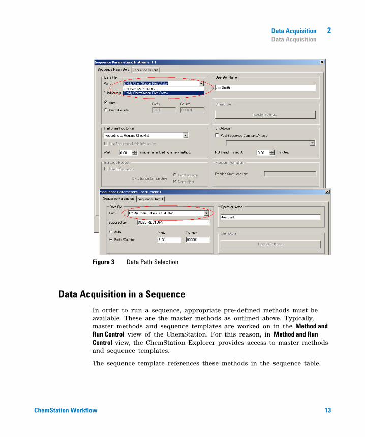
ChemStation Workflow 13
Data Acquisition 2Data Acquisition
Figure 3 Data Path Selection
Data Acquisition in a Sequence
In order to run a sequence, appropriate pre- defined methods must be available. These are the master methods as outlined above. Typically, master methods and sequence templates are worked on in the Method and Run Control view of the ChemStation. For this reason, in Method and Run Control view, the ChemStation Explorer provides access to master methods and sequence templates.
The sequence template references these methods in the sequence table.

14 ChemStation Workflow
2 Data AcquisitionData Acquisition
As explained previously, when a sequence is run with sequence template <sequence_name>.S, and the master method <method_name>.M is used, a new folder is created that contains all resulting files from the sequence run (“sequence container”).
The location of this folder is determined by the settings in the Sequence Parameters dialog box; the naming of this folder is determined by the Sequence tab of the Preferences dialog box. By default, the name is <sequence_name> <acquisition_date> <acquisition_time>, but it can be configured by using the tokens Operator, Instrument, Counter, and PC Name, or you can manually enter any name. If the Name Pattern would not result in unique names for the sequence containers, the ChemStation will append a counter to ensure uniqueness.
Figure 4 Preferences Dialog / Sequence Tab
At the start of an acquisition sequence, the method specified in the sequence table is copied from the master methods folder into the sequence container. In addition, a copy of the sequence is created and placed with the sequence log and the batch (*.b) file in the sequence container. All updates of the method (e.g. updates of the calibration table) are written to this sequence method in the container. All necessary files are now
ChemStation Workflow 15
Data Acquisition 2Data Acquisition
available for future data review and reprocessing, without changes that were applied to the master method or sequence template for other sequence runs.
During acquisition, the data files are stored to the sequence container. Within each data file (*.D), two additional methods, ACQ.M and DA.M, are saved for this specific run. These two methods are copies of the sequence method, preserving the state of the method as it was at the time of acquisition of the specific data file. In the case of e.g. calibration table updates the DA.M methods differ for each of the runs.
The individual acquisition method ACQ.M is intended to preserve the acquisition parameters, therefore it is recommended that you do not change this method during future data review activities. In Data Analysis view, the acquisition parameters of this method can be viewed and printed.
With these files saved in the sequence folder, all data review and reprocess activities can be performed without altering the master method or the sequence template. If needed, method changes can also be saved to the master method again.
Partial Sequence Acquisition
In the case of partial sequence acquisition, the user can decide between two options:
• acquire the partial sequence into a new sequence container
or
• acquire the partial sequence in an already existing sequence container.
Acquiring the data files from a partial sequence execution into an already existing sequence container may be useful in the following scenarios:
• A single data file (or several data files) have to be overwritten, because e.g. an incorrect vial was used in the first place.
• Only the first part of the sequence has been executed in the first place, and the missing samples have to be added by executing partial sequence. This may occur in the case of an instrument failure during sequence acquisition.

16 ChemStation Workflow
2 Data AcquisitionData Acquisition
• Additional lines have been added to the sequence template after acquisition of the already existing lines. The additional runs are to be added to the already existing data.
Therefore, when the user selects Partial Sequence from the Sequence menu, a dialog will come up providing him the option to either select an existing sequence container from a list or to create a new sequence container.
Figure 5 Partial Sequence Dialog
However, in order to maintain consistency of the sequence container (so it can be completely reprocessed in Data Analysis), only those sequence containers are offered for partial acquisition that fulfill certain conditions:
• The name of the sequence template (source sequence) and the name of the sequence .S file in the sequence container (target sequence) are identical.
• Both the data path and the subdirectory have to be identical for the sequence files.
• The number of sequence lines in the source sequence must be equal or higher than the number of sequence lines in the target sequence.
• For each line in the target sequence the sample type and the number of injections must be identical to the values in the corresponding lines of the source sequence.

ChemStation Workflow 17
Data Acquisition 2Data Acquisition
• The data file naming scheme must be identical for the two sequence files.
After leaving this dialog with Ok (for selecting one of the existing sequence data containers) or New (for creating a new sequence container), the user can select the sequence lines to be executed during partial sequence.
Data Acquisition of Single Runs
The new data concept is also introduced for single runs. In this case the data file is saved directly into the respective subdirectory. Since only one method is employed for a single run, this method does not need to be copied into the subdirectory; all actions are performed directly with the master method. After the acquisition part of the method is completed a copy of the master method is saved into the data file directory (ACQ.M). Another copy (DA.M) is saved after the data analysis part of the master method has been executed.

18 ChemStation Workflow
2 Data AcquisitionData Acquisition
19
ChemStation Workflow
Agilent Technologies
3Data Analysis
Data Analysis 20
Data Analysis: Data Review 23
The ChemStation User Interface during Data Review 30
Data Analysis: Reprocessing Data 32
This chapter outlines the data analysis and review options that are available, and explains how consideration of the data structure affects your choice of options.

20 ChemStation Workflow
3 Data AnalysisData Analysis
Data Analysis
Once the data have been acquired, they can be analyzed in ChemStation Data Analysis view. When selecting the Data tab of the ChemStation Explorer, you can load all the runs of a sequence or all single runs in a specific folder by double- clicking the corresponding symbol. The corresponding data set is then available in the Navigation Table.
Figure 6 Loading a Sequence from the ChemStation Explorer into Navigation Table
The main body of the navigation table consists of a list of all runs of the set. Instead of loading a run via the File > Load Signal menu, a run can now be loaded into ChemStation memory by double- clicking the relevant line in the navigation table. Additionally, a right- click on a run offers several options, e.g. to load or overlay specific signals from the file, to export the data, or to view the acquisition method parameters.
Once the run is loaded, you can review it, i.e. adjust data analysis parameters, integrate the signals and finally print a report. In this case you analyze the run as a single run without taking the sequence context into account or without using the features of the sequence table. This type of data analysis is called Data Review. The Navigation Table provides the tool set shown in Figure 7 on page 21, which makes data review more convenient.

ChemStation Workflow 21
Data Analysis 3Data Analysis
Figure 7 Data Review Toolset of the Navigation table
With this toolset, you can jump to the beginning or end of the navigation table, step on to next or previous run, automatically step through the runs, and stop automatic stepping.
A different way to analyze your data is to Reprocess a complete sequence. During this process, all runs are reanalyzed in the sequence context, i.e. the calibration tables of the sequence methods are updated in the case of calibration runs, multipliers, amounts etc. can be changed in the sequence table, new methods can be added to the sequence container, etc. For reprocessing, the navigation table provides the following toolset:
Figure 8 Sequence Reprocessing Toolset of the Navigation Table
Note that the reprocessing icons in the navigation table are available only for sequence data generated with ChemStation B.02.01 and higher. For single run data, for data generated prior to B.02.01, and for data acquired while Unique Folder Creation is switched off (see “Workflow with Unique Folder Creation switched off” on page 37), reprocessing in Data Analysis is not accessible. Such sequences need to be reprocessed in Method and Run Control, defining the sequence parameter Part of method to run as Reprocess Only. For sequences generated with ChemStation B.02.01 and higher, the reprocessing option in Method and Run Control has been removed (see Figure 9 on page 22), and the navigation table offers reprocessing as a Data Analysis Task.

22 ChemStation Workflow
3 Data AnalysisData Analysis
Figure 9 Sequence Parameters in Method and Run Control view of ChemStation B.02.01 and higher

ChemStation Workflow 23
Data Analysis 3Data Analysis: Data Review
Data Analysis: Data Review
Data Review means analyzing on a run- per- run base. ChemStation allows you to specify default actions that are performed automatically when a data file is loaded from the Navigation Table. These include data analysis tasks like integrating the chromatogram directly after loading, and also specifying the method that is to be loaded.
The corresponding options for reviewing (not used for reprocessing) are set up on the Signal/Review Options tab of the Preferences dialog box.
Figure 10 Preferences Dialog / Signal/Review Options Tab
The first section, Load Signal Options, specifies which of the signals in a run are loaded, and if the chromatograms are to be integrated and the results reported directly after loading.
In the second section, Data Review Options, you have the possibility to configure the interval for stepping through the runs in the navigation table automatically.

24 ChemStation Workflow
3 Data AnalysisData Analysis: Data Review
The remainder of this section specifies which method is loaded during data review when a run is loaded from the navigation table. They only apply to data review, but not to reprocessing. The following separate option sets are available for sequence runs and single runs:
Keep “Current Method”
The review setting Current Method should always be used when you want to use the method that is currently loaded. In this respect, for data review the current method remains irrespective of which single run data file or sequence container file is loaded. You can enable this option by selecting Current Method in the Preferences dialog, see Figure 11 on page 25. This ensures that, for each run loaded, the same method is always kept in memory.
Table 1 Data Review Options for Sequence and Single Run Data
Method used for review of sequence data Method used for review of single run data
Current Method Current Method
Sequence Method Individual method from data file (DA.M)
Individual method from data file (DA.M)
NOTE The options on the Signal/Review Options tab of the Preferences dialog are only applied when loading a data file from the Navigation Table. When using Load Signal from the File menu or the corresponding icon in the main tool bar, the settings are not applied, e.g. no method is loaded.
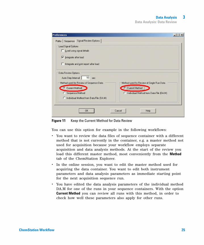
ChemStation Workflow 25
Data Analysis 3Data Analysis: Data Review
Figure 11 Keep the Current Method for Data Review
You can use this option for example in the following workflows:
• You want to review the data files of sequence container with a different method that is not currently in the container, e.g. a master method not used for acquisition because your workflow employs separate acquisition and data analysis methods. At the start of the review you load this different master method, most conveniently from the Method tab of the ChemStation Explorer.
• In the online session, you want to edit the master method used for acquiring the data container. You want to edit both instrument parameters and data analysis parameters as immediate starting point for the next acquisition sequence run.
• You have edited the data analysis parameters of the individual method DA.M for one of the runs in your sequence containers. With the option Current Method you can review all runs with this method, in order to check how well these parameters also apply for other runs.

26 ChemStation Workflow
3 Data AnalysisData Analysis: Data Review
Load “Sequence Method”
When you review the data using the option Sequence Method (see Figure 12 on page 26), each time you load a run from the Navigation Table, the sequence method corresponding to the run's sequence line is loaded. As the name of this option implies, it is only available for review of sequence data sets, but not of single runs.
Figure 12 Load the Sequence Method for Data Review
A typical application for this option is sequence- specific optimization of data analysis parameters, especially as preparation for reprocessing (see “Data Analysis: Reprocessing Data” on page 32). Once every run has been reviewed and the sequence methods have been improved, the complete sequence can be reprocessed with the updated methods.
It may be necessary to propagate the changes in the sequence method to the corresponding master method as input for all future acquisition runs. You can achieve this conveniently by e.g. using the Update Master Method functionality (see Table 3 on page 31).

ChemStation Workflow 27
Data Analysis 3Data Analysis: Data Review
Load “Individual Method from Data File (DA.M)”
The review setting Individual Method from Data File (DA.M) (see Figure 13 on page 27), should be used, if you want to load the individual DA.M automatically along with the corresponding data file, when this file is loaded using the navigation table. When you change a method and then load the next run, you will be asked to save your method changes, because you load a new method: the DA.M of the next run.
Figure 13 Load the Individual Method from Data File for Data Review
With the individual data analysis method (DA.M), it is possible to perform run- specific changes and save them in the individual data analysis method of the run. This may be useful in case of complicated chromatograms that require individual timed integration events for several runs of a sequence.
NOTE When a sequence is reprocessed, all actions are performed on the sequence methods and the DA.M of each data file is overwritten, including any changes you saved in these methods. Optimizing DA.M should be the last data analysis step after final reprocessing has already been performed.

28 ChemStation Workflow
3 Data AnalysisData Analysis: Data Review
Treatment of manual integration events
Manual integration events, e.g. a manually drawn baseline, are even more data file specific than timed integration events. In case of complicated chromatograms, it is highly desirable to be able to use these events for reprocessing.
Therefore, in ChemStation B.04.01 and higher, manual integration events can be stored directly in the data file instead of the method. At any time the data file is reviewed or reprocessed, the manual events in the data file are automatically applied. A run containing manual integration events is marked in the navigation table in the corresponding column.
In addition to the tools for drawing a baseline and deleting a peak manually, three additional tools are available in the user interface to
• Save manual events of the currently shown chromatograms into the data file,
• Remove all events from the currently shown chromatograms,
• Undo the last manual integration events (available until the event is saved).
When continuing to the next data file during review in the Navigation Table, ChemStation will check for unsaved manual integration events and ask the user whether he wants to save the events.
Manual events stored in the data file during review in the navigation table do not interfere with manual integration events stored during review in the Batch mode. These two ways of review are completely separated with regard to the manual events of a data file.
In ChemStation revisions prior to B.04.01, manual integration events could only be stored in the method. In B.04.01, this workflow can still be used. The Integration menu in Data Analysis view provides the following items in order to handle manual integration events with the method:
Update Manual Events of Method: Save newly drawn manual events to the method.
Apply Manual Events from Method: Apply the manual events currently saved in the method to the currently loaded data file.
Remove Manual Events from Method: Delete the manual events from the method.

ChemStation Workflow 29
Data Analysis 3Data Analysis: Data Review
In order to convert manual events stored in a method to storage in the data file, apply the events from the method and store the results in the data file. If wanted, remove the events from the method.
In case the Manual Events checkbox of the Integration Events Table of a method is enabled, the manual events of the method are always applied when loading a data file using this method. If the data file contains additional manual events, the events in the data file are used. When the Manual Events checkbox is enabled, the user is never asked to save the events to the data file.

30 ChemStation Workflow
3 Data AnalysisThe ChemStation User Interface during Data Review
The ChemStation User Interface during Data Review
The ChemStation user interface provides a number of features to facilitate working with the different methods available for data analysis (Figure 14 on page 30).
Figure 14 User Interface in Data Analysis
• The method modification status is displayed in Data Analysis view, so you can easily follow if there are unsaved method changes. The user interface always displays the name of the currently loaded method (together with the information whether it is an individual data analysis method of a data file or a sequence method).
• When you move the mouse pointer over this field, a tool tip additionally displays the complete path and name of the method.
• A dropdown box provides a shortcut to the method options of the Preferences dialog. You can directly enable any of the available options and it will be applied the next time you load a run from the Navigation Table. Moreover, it is also very convenient to see which option is currently active. Note that these options only apply to data review, but not to reprocessing.
Saving methods in Data Analysis view
During work in Data Analysis view, the user optimizes the data analysis parameters of his methods. In addition to just saving a method, the workflow may also require e.g. to save a sequence method with different name or as a master method into the master method directory.
The Method menu in data analysis provides several items to save the method:

ChemStation Workflow 31
Data Analysis 3The ChemStation User Interface during Data Review
The option Save as new Master Method for sequence methods and individual methods DA.M per default have the master method directory preselected as the target directory.
Update master method feature
In addition, the Method menu provides the possibility to make available for the sequence or master method only the data analysis parameters you developed for the individual method. This option, Update Master Method or Update Sequence Method is available from the Method menu or via a right- click in the Navigation Table on the corresponding run.
This feature is available in the following situations:
Table 2 Save Options of the Method Menu in Data Analysis View
Method Loading Preference Available Save Options
Current Method Save Method
Save Method As
Sequence Method Save Sequence Method
Save as new Master Method
Individual method from data file Save Data File Method
Save as new Master Method
Table 3 Availability of the Update … Method Functionality
Loaded Method Available Options
Individual data analysis method (DA.M) Update Master MethodUpdate Sequence Method
Sequence method Update Master Method
Master method —
NOTE It is important to note that this feature only updates data analysis parameters of the target method, and that it overwrites all data analysis parameters. For technical reasons, in addition to the data analysis parameters, the Audit Trail of the target method is also overwritten with the Audit Trail of the source method.
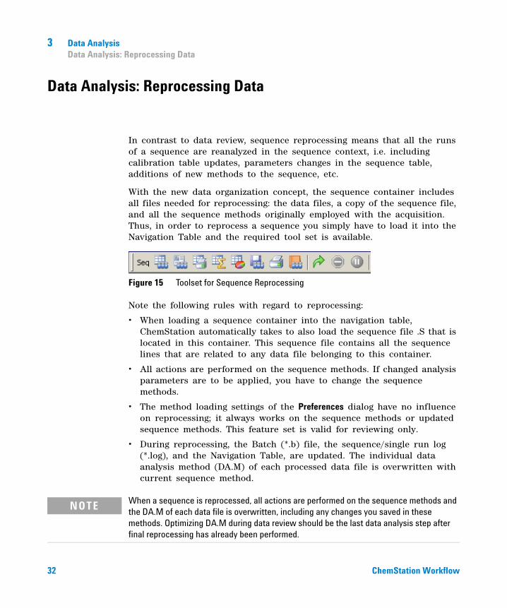
32 ChemStation Workflow
3 Data AnalysisData Analysis: Reprocessing Data
Data Analysis: Reprocessing Data
In contrast to data review, sequence reprocessing means that all the runs of a sequence are reanalyzed in the sequence context, i.e. including calibration table updates, parameters changes in the sequence table, additions of new methods to the sequence, etc.
With the new data organization concept, the sequence container includes all files needed for reprocessing: the data files, a copy of the sequence file, and all the sequence methods originally employed with the acquisition. Thus, in order to reprocess a sequence you simply have to load it into the Navigation Table and the required tool set is available.
Figure 15 Toolset for Sequence Reprocessing
Note the following rules with regard to reprocessing:
• When loading a sequence container into the navigation table, ChemStation automatically takes to also load the sequence file .S that is located in this container. This sequence file contains all the sequence lines that are related to any data file belonging to this container.
• All actions are performed on the sequence methods. If changed analysis parameters are to be applied, you have to change the sequence methods.
• The method loading settings of the Preferences dialog have no influence on reprocessing; it always works on the sequence methods or updated sequence methods. This feature set is valid for reviewing only.
• During reprocessing, the Batch (*.b) file, the sequence/single run log (*.log), and the Navigation Table, are updated. The individual data analysis method (DA.M) of each processed data file is overwritten with current sequence method.
NOTE When a sequence is reprocessed, all actions are performed on the sequence methods and the DA.M of each data file is overwritten, including any changes you saved in these methods. Optimizing DA.M during data review should be the last data analysis step after final reprocessing has already been performed.

ChemStation Workflow 33
Data Analysis 3Data Analysis: Reprocessing Data
• If you want to add new methods from one of the master method directories to the sequence table, use the Browse item in the list of methods to browse to any specified method directory (only the methods already in the sequence container are available without browsing). The new method is copied to the sequence container during reprocessing. This implies that you cannot select a method with the same name as a method already present in the container.
Figure 16 Browse to the Master Methods directory in the Sequence Table
• In the sequence table, it is not possible to add or remove lines.
• In the Sequence Parameters dialog, only the operator name, the sequence comment, and the usage of sequence table information can be changed. All other fields have to be set during data acquisition or do not apply to reprocessing.

34 ChemStation Workflow
3 Data AnalysisData Analysis: Reprocessing Data
Figure 17 Sequence Parameters in Data Analysis
Saving Sequences in Data Analysis View
The Sequence menu provides the possibility to save the sequence after modifying the sequence table, sequence parameters, or sequence output parameters. In addition it allows you to save a data analysis sequence (that is stored with sequence container) as a sequence template. This functionality may be useful if you have added sequence lines to the sequence table during acquisition. These additional lines are only available in that specific sequence container, but not in the original sequence template.
Saving a sequence as new sequence template automatically converts the sequence file so that all fields are editable again.

35
ChemStation Workflow
Agilent Technologies
4Workflow with Unique Folder Creation switched off
Working with "Unique Folder Creation" on or off? 36
Workflow with Unique Folder Creation switched off 37
Sequence Container Migration 41
This chapter provides information on working with Unique Folder Creation switched off which allows you to store data as in ChemStation revisions B.01.03 or earlier. This mode does not take full advantage of the latest data review and reprocessing functionality in ChemStation.

36 ChemStation Workflow
4 Workflow with Unique Folder Creation switched offWorking with "Unique Folder Creation" on or off?
Working with "Unique Folder Creation" on or off?
The new data concept as outlined in the previous chapters provides a number of advantages:
• Sequence data are not overwritten. Each sequence acquisition stores the resulting data files in its own sequence container with unique name.
• With the sequence container concept, the data are stored with all necessary information needed for data analysis, i.e. copies of the sequence file and of all methods employed with the sequence. These methods can be changed with sequence specific input and do not influence the original master method. The container concept thus strengthens the meaning of a sequence as a set of data files and methods belonging together for result creation.
• Data review and reprocessing are both available in Data Analysis view via the Navigation Table.
• The data container concept provides the optimal preconditions for the ChemStation OpenLAB Option, allowing to exchange data with the Agilent OpenLAB Enterprise Content Manager (ECM).
However, there may be situations where users may want to store their data as in ChemStation B.01.03 or earlier and work according to the corresponding workflows:
• During method development it may be more convenient to have only one method for both acquisition and data analysis to automatically have changes available for future acquisition and reanalysis of already acquired data.
• Data from several acquisitions have to be in one folder, e.g. in case of partial acquisition.
• Customized macro solutions on a ChemStation system that have been designed for older revisions may require the data, methods, or sequence to be stored according to the old data organization scheme.
• When ChemStation B.04.01 runs in a lab where there are also system still running on ChemStation revisions B.01.03 or earlier, it may be more convenient to use the same data organization mode on all systems.

ChemStation Workflow 37
Workflow with Unique Folder Creation switched off 4Workflow with Unique Folder Creation switched off
Workflow with Unique Folder Creation switched off
In order to allow working with a data storage concept as in ChemStation revisions before B.02.01, the Sequence tab of the Preferences dialog box a Data Storage section. Here you can choose between Unique Folder Creation ON and Unique Folder Creation OFF (Figure 18 on page 37). Per default, Unique Folder Creation ON is selected. Unique Folder Creation ON enables the data storage concept as outlined in the three chapters above.
Figure 18 Preferences Dialog / Sequence Tab
NOTE Switching Unique Folder Creation on or off only affects future acquisitions, but does not change the data organization of already acquired data.
NOTE We recommend to decide between the two modes at the beginning of your work and not to switch between them.
Switching Unique Folder Creation off is not supported with the ChemStation OpenLAB Option or ChemStore/Security Pack installed.

38 ChemStation Workflow
4 Workflow with Unique Folder Creation switched offWorkflow with Unique Folder Creation switched off
Selecting Unique Folder Creation Off has the following impact on data storage:
• Sequence data are not acquired into a sequence container, but directly into the subdirectory as specified in the Sequence Parameters ( Figure 4 on page 14). Therefore, the sequence name pattern is grayed out on the Sequence tab of the Preferences dialog ( Figure 18 on page 37).
• This means that for two or more sequence acquisitions the data may be acquired into the same subdirectory. This implies the risk to overwrite existing data, but on the other hand allows to split sequences using partial sequence execution and still combine the results in one folder (which would not be possible with Unique Folder Creation switched on).
• No sequence methods (.M) or copies of the sequence file (.S) are stored with the data, but only the sequence logfile and the batch file (.B). This means only the methods and sequences in the paths specified in the Preferences dialog ( Figure 2 on page 12) are available. They have to be used for acquisition as well as for data review and reprocessing. Sequence or data file specific method changes can only be stored by saving the method with different name. Otherwise these changes are also applied to the acquisition method. On the other hand, this may be desired behavior during method development.
• There are no data file specific methods ACQ.M and DA.M stored. Saving information about the original acquisition is only possible by including this information in the report or by selecting Save Method with Data from the method’s runtime checklist (Figure 19 on page 39). With this option the acquisition method will be stored as RUN.M in each data file.

ChemStation Workflow 39
Workflow with Unique Folder Creation switched off 4Workflow with Unique Folder Creation switched off
Figure 19 Run Time Checklist: Save Method with Data
The enhanced ChemStation user interface as introduced with ChemStation B.02.01 is also available when Unique Folder Creation is switched off. However, there are functions you can not take advantage of in this mode. The same limitations also apply to any run acquired with ChemStation prior to B.02.01.
• When a sequence is loaded into the Navigation Table, the reprocessing toolset is grayed out (Figure 20 on page 39). Sequences that have been acquired in this data storage mode can only be reprocessed in Method and Run Control view using the Reprocessing only option in the Sequence Parameters (Figure 21 on page 40).
Figure 20 Navigation Table for Sequences acquired with Unique Folder Creation switched off

40 ChemStation Workflow
4 Workflow with Unique Folder Creation switched offWorkflow with Unique Folder Creation switched off
Figure 21 Reprocessing of sequence data acquired with Unique Folder Creation off
• With the method usage options Individual Method from Data File and Sequence Method (see Figure 10 on page 23), a warning message will be displayed each time a run is double- clicked in the Navigation Table that the individual method/sequence method does not exist. As outlined above, these methods are not stored with the data. In this case, the only meaningful option for data review is Current Method.

ChemStation Workflow 41
Workflow with Unique Folder Creation switched off 4Sequence Container Migration
Sequence Container Migration
ChemStation provides a tool to migrate non- container data to sequence container format. To successfully perform this task, it is required that the original sequence file is still available. It must contain all the necessary sequence lines and follow the original data file naming scheme to reprocess all the data files of the sequence. In addition, all the methods in the Method column of the sequence table have to be available.
To perform migration,
start the Sequence Container Migration from the Sequence menu in Data Analysis view.
Figure 22 Sequence Container Migration
Fill in the following required fields (see Figure 22 on page 41):
Select Sequence Template: Select the sequence file .S that contains the sequence table that matches the data set to be migrated.
Select Method Patch: Select the directory where the methods are located that are referenced in the sequence table.
42 ChemStation Workflow
4 Workflow with Unique Folder Creation switched offSequence Container Migration
Select Source: Select the directory that contains the data files to be migrated.
Select Destination: Specify the path and name of the sequence container to be created. You may select an existing folder or create a new one.
When all fields are filled in, the migration can be started.
The following steps will be performed:
• The sequence container directory will be created.
• The sequence template will be copied to the container. It will also be converted to a state where it is able to reprocess data files in Data Analysis view.
• The methods referenced in the sequence table are copied from the specified method path to the container folder.
• The data files, the sequence logbook, and the batch file are copied from the data source directory to the destination directory.
• According to the information in the sequence table, a copy of the corresponding method is copied to each data file as DA.M.
When the container migration is completed, a success message is displayed in the Messages and Warnings field. Otherwise a warning message indicates any problem during migration. Details about the warning can be obtained by double- clicking the warning message.

ChemStation Workflow 43
Workflow with Unique Folder Creation switched off 4Sequence Container Migration

© Agilent Technologies 2006, 2007-2010
Printed in Germany 2/2010
*G2170-90044**G2170-90044*G2170- 90044
www.agilent.com
Agilent Technologies
In This Book
With ChemStation revision B.02.01 or higher, data review and data reprocessing capabilities have been significantly improved to enable fast review of result data.
The new data storage functions in ChemStation help to efficiently organize sequence data and methods.

Agilent ChemStation for UV-visible Spectroscopy
Operator’s Manual for Biochemical Analysis Software
s1

Biochemical Analysis Software for Agilent ChemStation
Notices© Agilent Technologies, Inc. 2002, 2003-2008
No part of this manual may be reproduced in any form or by any means (including elec-tronic storage and retrieval or translation into a foreign language) without prior agree-ment and written consent from Agilent Technologies, Inc. as governed by United States and international copyright laws.
Manual Part NumberG1117-90022
Edition07/08
Printed in Germany
Agilent Technologies Hewlett-Packard-Strasse 876337 Waldbronn
Research Use OnlyNot for use in Diagnostic Procedures.
WarrantyThe material contained in this docu-ment is provided “as is,” and is sub-ject to being changed, without notice, in future editions. Further, to the max-imum extent permitted by applicable law, Agilent disclaims all warranties, either express or implied, with regard to this manual and any information contained herein, including but not limited to the implied warranties of merchantability and fitness for a par-ticular purpose. Agilent shall not be liable for errors or for incidental or consequential damages in connec-tion with the furnishing, use, or per-formance of this document or of any information contained herein. Should Agilent and the user have a separate written agreement with warranty terms covering the material in this document that conflict with these terms, the warranty terms in the sep-arate agreement shall control.
Technology Licenses The hardware and/or software described in this document are furnished under a license and may be used or copied only in accor-dance with the terms of such license.
Restricted Rights LegendIf software is for use in the performance of a U.S. Government prime contract or subcon-tract, Software is delivered and licensed as “Commercial computer software” as defined in DFAR 252.227-7014 (June 1995), or as a “commercial item” as defined in FAR 2.101(a) or as “Restricted computer soft-ware” as defined in FAR 52.227-19 (June 1987) or any equivalent agency regulation or contract clause. Use, duplication or disclo-sure of Software is subject to Agilent Tech-nologies’ standard commercial license terms, and non-DOD Departments and Agencies of the U.S. Government will receive no greater than Restricted Rights as
defined in FAR 52.227-19(c)(1-2) (June 1987). U.S. Government users will receive no greater than Limited Rights as defined in FAR 52.227-14 (June 1987) or DFAR 252.227-7015 (b)(2) (November 1995), as applicable in any technical data.
Safety Notices
CAUTION
A CAUTION notice denotes a haz-ard. It calls attention to an operat-ing procedure, practice, or the like that, if not correctly performed or adhered to, could result in damage to the product or loss of important data. Do not proceed beyond a CAUTION notice until the indicated conditions are fully understood and met.
WARNING
A WARNING notice denotes a hazard. It calls attention to an operating procedure, practice, or the like that, if not correctly per-formed or adhered to, could result in personal injury or death. Do not proceed beyond a WARNING notice until the indicated condi-tions are fully understood and met.

In This Guide…The biochemical analysis software for Agilent ChemStation adds the kinetic mode and the thermal denaturation mode to the general purpose software. These two modes enable you to perform kinetic experiments and thermal denaturation experiments with the Agilent 8453 spectrophotometer. This includes capabilities to develop analytical methods, real time online monitors to view your ongoing experiments, and tools to evaluate and process the experimental data.
This book gives you instructions for the installation of the software and hardware components needed for kinetic and thermal denaturation experiments. Further, you get information about the most important software features, which will help you to solve your analytical problems.
This manual is organized in three chapters, which lead you from the installation of the software to the evaluation and presentation of a kinetic or a thermal denaturation experiment.
1 Installation and Configuration
This chapter describes the installation of the Agilent ChemStation software and the configuration of the Agilent 89090A Peltier temperature controller, which is needed for thermal denaturation experiments.
2 Kinetics Mode
This chapter leads the user form the configuration of the spectrophotometer and the sampling system, the development of a kinetic method to the kinetic measurement and finally the evaluation of the experimental data.
3 Thermal Denaturation Mode
This chapter describes the setup of a temperature ramp and an analytical method in order to perform a thermal denaturation experiment. The user will learn about the online monitor of the experiment and the possibilities for data evaluation with the software.
Biochemical Analysis Software for Agilent ChemStation 3

4 Biochemical Analysis Software for Agilent ChemStation

Contents
1 Installation and Configuration 7
Installing the Biochemical Analysis Software 8
Configuring your Agilent 89090A Peltier Temperature Controller 9
2 Kinetics Mode 11
Preparing a Time Based Measurement 12
Starting the Kinetics Mode 12Setting Up your Spectrophotometer 14Configuring the Sampling System 16Setting Up a Kinetic Method 18
The Kinetic Measurement 23
Running a Time Based Measurement 23Evaluating your Kinetic Data 24Viewing Results 26
3 Thermal Denaturation Mode 27
Preparing a Thermal Denaturation Measurement 28
Starting the Thermal Denaturation Mode 29Setting Up your Spectrophotometer 30Setting Up the Temperature Ramp 30Setting Up a Thermal Denaturation Method 31
The Thermal Denaturation Experiment 36
Running a Thermal Denaturation Experiment 36Evaluating your Thermal Denaturation Data 37Viewing Results 38
Biochemical Analysis Software for Agilent ChemStation 5

Contents
Index 39
6 Biochemical Analysis Software for Agilent ChemStation

Agilent ChemStation for UV-visible SpectroscopyOperator’s Manual for Biochemical Analysis Software
1Installation and Configuration
Installing the Biochemical Analysis Software 8
Configuring your Agilent 89090A Peltier Temperature Controller 9
Before you can use the biochemical analysis software, you have to install the software and configure the spectrophotometer. In this chapter the tools and the procedures for the installation are described. First, the biochemical analysis software has to be installed on your Agilent ChemStation.
If you want to use the thermal denaturation mode of Agilent ChemStation you also have to configure the Agilent 89090A peltier temperature controller. This installation is optional for the kinetics mode.
7Agilent Technologies

1 Installation and Configuration
Installing the Biochemical Analysis Software
The biochemical analysis software (G1117A) is an add-on module and is based on the general purpose software (G1115A). For details of the installation please see your Agilent 8453 UV-visible Spectroscopy System - Installation Guide.
If you want to add the Biochemical Analysis software package please follow the steps below.
1 Insert your Agilent UV-visible ChemStation CD-ROM.
2 Start setup.exe.
3 Select Modify and press Next.
4 Check G1117AA/G1123AA Biochemical Add-On and press Next.
5 Enter the license number for your Biochemical Analysis software and press Add License.
6 Press Next and wait until the Maintenance Complete dialog is displayed and press Finish.
7 After the installation is completed, run Installation Qualification, which is available in the UV-Visible ChemStations menu.
8 If the Installation Qualification is successfully completed, the biochemical analysis software is ready to use.
8 Biochemical Analysis Software for Agilent ChemStation

Installation and Configuration 1
Configuring your Agilent 89090A Peltier Temperature Controller
If you are planing to use the thermal denaturation mode of your biochemical analysis software, you have to configure the Agilent 89090A Peltier temperature controller.
1 Start the UV-Vis Configuration Editor from the UV-Visible ChemStations Menu.
2 If no Agilent 8453 Instrument has been configured yet, add New Instrument as described in the Agilent 8453 UV-visible Spectroscopy System Operator’s Manual.
3 Select Instruments… from the Configure Menu.
4 Enter Instrument Name, choose the Initial Screen Window Size and click OK.
5 From the UV-Vis Modules list select TemCo.
6 Set an GPIB address of 20.
7 Press Add to add the Peltier Temperature controller to your current configuration.
8 Press OK to close the Device Configuration dialog box.
9 Use the Exit command from the File menu to quit the Configuration Editor.
10 Press Yes to save your configuration before exiting.
Biochemical Analysis Software for Agilent ChemStation 9

1 Installation and Configuration
10 Biochemical Analysis Software for Agilent ChemStation

Agilent ChemStation for UV-visible SpectroscopyOperator’s Manual for Biochemical Analysis Software
2Kinetics Mode
Preparing a Time Based Measurement 12
The Kinetic Measurement 23
In this chapter the most important tasks in the kinetic mode of the biochemical analysis software will be described. Since good preparation is essential for a kinetic measurement, the first section, “Preparing a Time Based Measurement" on page 12, contains information about the steps before the kinetic measurement. You will learn how to setup the spectrophotometer, the sampling system and an analytical method.
The second section, “The Kinetic Measurement" on page 23, describes the actual time based measurement and the possibilities for data processing as well as data evaluation with the Agilent ChemStation software.
11Agilent Technologies

2 Kinetics Mode
Preparing a Time Based Measurement
Before you perform a time based measurement you have to setup your system according to your application. In this section you will learn to setup your spectrophotometer, to select and setup the a sampling system and to develop a kinetic method. This will enable you to use the features of the biochemical analysis software in order to find the best solution for your kinetic measurement.
Starting the Kinetics Mode
To start the kinetics mode of the biochemical analysis software choose Kinetics in the Mode menu or in the mode drop down box of the graphical user interface.
Figure 1 shows the graphical user interface for the kinetics mode of the Agilent ChemStation software. The current mode is shown in the mode drop down box on the Toolbar. The Toolbar also includes the method name field, where the name of the actual analytical method is displayed. The letters Mod next to the method name field indicate that this method has been modified and that these modifications have not been stored yet. The Toolbar also includes several shortcut buttons, which are described in detail in the Agilent 8453 UV-visible Spectroscopy System Operator’s Manual.
12 Biochemical Analysis Software for Agilent ChemStation

Kinetics Mode 2
The SideBar is divided into two parts. The (upper) analytical panel includes a Setup… button, which opens the method dialog box. This dialog box includes the most important method parameters. In the (lower) instrument panel you can select the sampling system and switch the lamps of the spectrophotometer.
The default graphical user interface in the kinetic mode contains the Time Trace window, the Results window and the Method Summary window. In these windows the kinetic time traces, the evaluated kinetic data and the core method parameters are displayed after the measurement.
Figure 1 The Graphical User Interface of the Kinetics Mode
Biochemical Analysis Software for Agilent ChemStation 13

2 Kinetics Mode
Setting Up your Spectrophotometer
Select the Instrument menu of the biochemical analysis software to setup your Agilent 8453 spectrophotometer for a time-based measurement.
Choose Setup Spectrophotometer… to display the Instrument Parameters dialog box, which allows you to set the run-time parameters for the spectrophotometer. In this dialog box you can set the following parameters.
• You can use the fields to specify lower and upper limits of the range required by your analysis. The From field defines the lower limit of the range, the To field defines the upper limit of the range. The default values are the wavelength range limits of the configured spectrophotometer.
NOTE It is recommended to use the maximum wavelength range of your spectrophotometer. This enables you to use the full benefits of the diode array spectrophotometer, for example, post run data evaluation at different wavelengths.
14 Biochemical Analysis Software for Agilent ChemStation

Kinetics Mode 2
• The value in the Integration time field is the time in seconds over which the signal is collected and integrated. The Integration time must be between 0.1 and 25.5 seconds; the default is 0.5 seconds. Longer Integration times improve the signal-to-noise ratio since signal is accumulated while noise is averaged out. The selected integration time has a direct impact on the minimum cycle time for a kinetic measurement. The minimum cycle time cannot be shorter than the integration time. Hence, it might be necessary to minimize the Integration time for fast kinetic measurements.
• The number in the Interval field defines the wavelength measurement interval. The minimum interval is 1 nm, corresponding with the highest resolution.
Select Lamp(s)… to display the Lamp(s) Parameter dialog box. It allows you to set the parameters of the spectrophotometer's lamp(s). The format of the Lamp(s) Parameter dialog box depends upon the spectrophotometer type. With 8453 spectrophotometer you have the option to switch the deuterium lamp and the tungsten lamp On and Off. The lamps can also be switched by clicking on the lamp icons in the Instrument panel of the SideBar of the graphical user interface.
The actual status of the spectrophotometer instrument is summarized in the Spectrophotometer Status window. In this window the following actual values are displayed:
Instrument type, wavelength range, wavelength interval, integration time, power on time, the status of the lamp(s) and the overall status of the Agilent 8453 spectrophotometer (ready/not ready).
NOTE It is recommended not to change the default value of 1 nm in order to achieve the optimum performance of the spectrophotometer
NOTE If you change the lamp parameters, the current method is modified and the lamp status is changed. In the case of a lamp failure (ignition failure, lamp defect or lamp door open), the lamp(s) parameters may be displayed as On, although the lamp(s) are off. Check the actual status of the lamp(s) in the Spectrophotometer Status window or the Instrument panel of the SideBar of the graphical user interface.
Biochemical Analysis Software for Agilent ChemStation 15
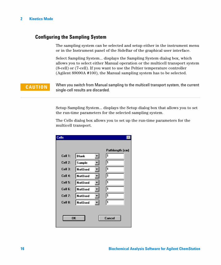
2 Kinetics Mode
Configuring the Sampling System
The sampling system can be selected and setup either in the instrument menu or in the Instrument panel of the SideBar of the graphical user interface.
Select Sampling System… displays the Sampling System dialog box, which allows you to select either Manual operation or the multicell transport system (8-cell) or (7-cell). If you want to use the Peltier temperature controller (Agilent 89090A #100), the Manual sampling system has to be selected.
Setup Sampling System… displays the Setup dialog box that allows you to set the run-time parameters for the selected sampling system.
The Cells dialog box allows you to set up the run-time parameters for the multicell transport.
CAUTION When you switch from Manual sampling to the multicell transport system, the current single-cell results are discarded.
16 Biochemical Analysis Software for Agilent ChemStation

Kinetics Mode 2
The dialog box contains the used cells as table with the following columns:
• Cell n: indicates the cell positions in the multicell transport; cell 1 is the cell nearest the front of the spectrophotometer.
• The central column of the table describes the sample in the cell. Choose Sample, Blank or Not Used from the drop-down list.
• The Path Length fields show the path lengths in centimeter of the sample cells in each position of the multicell transport. The default value for each cell is 1 cm.
The Single Cell dialog box allows you to set up the run-time parameters for manual operation.
The Path Length field the path length in cm of the sample cell you are using has to be edited The default value is 1 cm.
Select Wait for Temperature Ready to ensure that the Agilent ChemStation waits for a Ready signal from the Agilent 89090A Peltier temperature control accessory before making a measurement. The default condition is cleared. This check box is only available, when the Agilent 89090A Peltier temperature controller is configured.
NOTE It is good measurement practice to use position 1 for the Blank measurement. Then the Blank spectrum is always renewed at the beginning of a measurement cycle. This becomes especially important, if you performing long time kinetic experiments.
Biochemical Analysis Software for Agilent ChemStation 17

2 Kinetics Mode
Setting Up a Kinetic Method
Method parameters are edited in the Time & Calculation dialog box and the Info & Options dialog box under the Method menu. The Time & Calculation dialog box is also displayed, when Setup button has been pushed. The most important parameters of your method are displayed in the Method Summary window of your graphical user interface.
In the Time & Calculation dialog box you can define the conditions for the time based measurement.
18 Biochemical Analysis Software for Agilent ChemStation

Kinetics Mode 2
• The Use Wavelength field allows you to define the wavelength (for multicell measurements) or up to six wavelengths (for single cell measurements) of your processed data from which the amplitude values are extracted for the wavelength result. The default wavelength is 480 nm. If you enter wavelengths at which no measured data are available (for example non-integer values), the amplitude values are calculated by linear interpolation.
• The Background Correction field allows you to specify any background correction that is applied to the wavelength result to calculate a function result. Choose the down arrow and select a background correction procedure from the drop-down list:
none — specifies that the wavelength result is used as measured without background correction.
single reference wavelength — specifies that the absorbance at a single wavelength is subtracted from the wavelength result. You specify the background wavelength in the field.
subtract average over a range — specifies that the average absorbance over a wavelength range is subtracted from the wavelength result. You specify the upper and lower limits of the background wavelength range in the fields.
three-point drop-line — specifies that a background absorbance calculated using a three-point drop-line is subtracted from the wavelength result. You specify the upper and lower limits of the background wavelength range used for the background calculation in the adjacent left (lower) and right (upper) fields.
• The Trace Monitor is a continuously-updated time trace that shows the change of absorbance at the wavelength specified in the Use Wavelength field with time. Define the scaling of the absorbance (y) axis by typing lower and upper limits in the Y scaling from: and to: fields.
• You can choose to monitor either the last acquired spectrum or spectra from a specific cell. Choose the down arrow and select either Last Spectrum, Cell n (for multicell measurements) or All Spectra (for single cell measurements). Define the scaling of the absorbance (y) axis by typing lower and upper limits in the Y scaling from: and to: fields.
• The Run Time is the total time of the analysis. The Run Time range is up to 999999 seconds (11.5 days). The Run Time must be greater than Cycle Time plus Start Time.
Biochemical Analysis Software for Agilent ChemStation 19

2 Kinetics Mode
• The Start Time is the time between initiating measurement and measurement starting, and is optional. The default value is 0.0.
• The Cycle Time is the time from the start of one measurement to the start of the next; the default value is 5.0 seconds for multicell operation, 0.5 seconds for single cell operation (minimum acceptable values).
• The minimum cycle time is hardware-dependent, and the value given is an approximation only. To avoid losing data, you must determine the minimum cycle time for your configuration experimentally. The minimum cycle time depends on the sampling system (number of measurements per cycle), the integration time (defined in the Setup Spectrophotometer… dialog box) and the stray light correction (defined in the Info & Options dialog box).
• Select Increment cycle time to activate the increase in cycle time. Specify the percentage increase in the % field and a time interval (in seconds) in the after initial time of: field.
• You can choose from five different kinetic evaluation types. Choose the down arrow and select the calculation type from the drop-down list:
None — specifies that no rate calculation is made.
Initial rate — specifies that a quadratic fit is made according to the equation, a+bt+ct2 where b is the initial rate constant.
Zero order — specifies that a linear fit is made according to the equation,a + bt where b is the rate constant in AU/s.
First order — specifies that an exponential fit is made according to the equation,a+b·exp(-kt) where k is the rate constant in 1/s.
Delta AU — specifies a subtraction of the starting absorbance from the final absorbance:Abst(end) - Abst(start)
• You can specify that the rate calculation is made over a limited time range. Type the start time for the calculation in the from: field and the end time in the to: field.
• Select Multiply Rate to activate a conversion factor for the rate result. Specify the factor and the new units in the to convert to Rate unit: field.
Select Subtract Rate of Cell to subtract the result of a reference cell from the rate results of all other cells. Choose the down arrow and select the reference cell from the drop-down list. This option is available only when you have configured a multiple-cell measurement.
20 Biochemical Analysis Software for Agilent ChemStation

Kinetics Mode 2
In the Options & Information dialog box you can define the acquisition conditions for the kinetics experiment.
• Move multicell transport for stirring if possible will move the current cell into position for sample stirring during the idle time between two cycles, if the cycle time is sufficiently long (approximately the minimum cycle time plus 4 seconds for each configured cell). This check box is available only when a multicell transport system is selected.
• Adjust gains separately from blank measurement adds the Set Gains command into the Measure menu. Set Gains performs a gain adjustment, reference and a measurement; the Blank command performs a reference and a measurement only. The separate gain adjustment on a blank medium with high transmission (for example, water or buffer) sets the gains to a lower value in order avoids an A/D converter overflow and invalid data points due to negative slope time traces.
Biochemical Analysis Software for Agilent ChemStation 21

2 Kinetics Mode
• Stray light Correction On switches stray light correction option. When stray light correction is on, a second measurement is made with the starlight filter in place, and the sample spectrum is corrected for stray light using this spectrum. The stray light correction increases the minimum cycle time by the Integration Time (set in the Instrument Parameters dialog box) plus 2 seconds.
• Check Autosave spectra to file to save all acquired spectra to disk. Type a name for the file in the adjacent field. The spectra are stored in the default directory (CHEM32\n\DATA) with the .KD extension. The default directory can be changed in the Config menu
• Prompt for sample information before run will display the Sample Information dialog box before measurements are started.
• Select Start Run on Trigger to start data acquisition using a closure of contacts 13 and 15 of the GPIO interface. This ensures that minimum time elapses (approximately 0.12 seconds) between the trigger action and the start of data acquisition; it is intended to be used for fast reaction kinetics.
• You can type a description of the method in the Method Information field. The field accepts any alphanumeric characters, and the description can be as long as you wish. The text wraps automatically at the end of the line. You can edit an existing description using any of the standard text-processing procedures (for example, Copy, Cut, Paste).
22 Biochemical Analysis Software for Agilent ChemStation

Kinetics Mode 2
The Kinetic Measurement
Running a Time Based Measurement
Measurements can be started either by using the Measure menu from the menu bar, by pushing the buttons (Blank, Sample, Time Based Measurement) on the SideBar of the graphical user interface or by using selected F keys.
If you have selected the option Adjust gains separately from blank measurement in the Options & Info… dialog box, Set Gains is included in the Measure menu. The separate gain adjustment on a blank medium with high transmission (for example, water or buffer) sets the gains to a lower value and avoids an A/D converter overflow. This helps to avoid invalid data points due to negative slope time traces.
1 Introduce cell filled with water or any other low absorbing medium into the cell holder.
2 Move multicell transport to the right position.
3 Click on Set gains in the Measure menu.
With a multicell sampling system it is recommended to measure Zero Cell spectra in order to correct for slightly different optical properties of the measurement cells. You should initialize the multicell transport with identical blank medium in all cells. The Zero Cells… command measures a true blank spectrum for cell 1, then measures spectra for the remaining cells. The difference spectra is obtained by subtracting the blank spectrum from the individual cell spectra are then subtracted automatically from all subsequent measured spectra to correct for any cell-to-cell optical differences.
1 Fill all measurement cells with the same blank medium (for example, water).
2 Make sure, that there are no bubbles or floating particles in the cells.
3 Do a Blank measurement by selecting Blank in the measurement menu, by clicking the Blank Button on the SideBar of the graphical user interface or by using F4.
4 Start the Zero Cells measurement from the Measure menu.
The Zero cell spectra are displayed in the Zero Cells Spectra window, which can be activated in the view menu. Make sure that you do not switch the cells after the zero cell measurement.
Biochemical Analysis Software for Agilent ChemStation 23

2 Kinetics Mode
To measure a single spectrum of the solution in the cell and display it in the Sample Spectra window select Sample (Single Spectrum) in the measure menu. You can also measure a single spectrum by pressing F5 or the Sample Button in the SideBar of the graphical user interface.
Pressing F7, selecting time based measurement from the measure menu or from the SideBar of the graphical user interface prepares the software for starting the time based measurement. Now the Time Trace window and the Sample Spectra window are displayed. Choose Start from the new menu bar to start the acquisition or Abort to abort an acquisition in progress.
During the Time Based Measurement you can follow the acquisition of the spectra and the time traces in real-time in the Time Trace window and the Sample Spectra window. Use the left double-click on the mouse in the Time Trace window area or the Sample Spectra window area to autoscale the y-axis.
After the Time Based Measurement has been finished or aborted by the user, the kinetic data are stored as specified in the Options & Info… dialog box. The Time traces are evaluated by the rate type, which has been defined in the Time & Calculation dialog box. These results are displayed in the Results window.
Evaluating your Kinetic Data
After the time based measurement has been finished you have the possibility to reevaluate the kinetic data. Since full spectra have been acquired during the measurement, the parameters in the fields Wavelength and Rate Calculation of the Time & Calculation dialog box can be changed. Click on OK to make the changes active. The new results are displayed in the Results window. If the method parameter has been changed the modified flag Mod will appear on the graphical user interface.
If manual sampling system has been configured, you can choose Edit Sample Information from the Results window to display the Sample Information dialog box. It allows you to include sample information with your results. The Sample Information dialog box contains the following parameters:
• The Sample Name.
• A comment (for example a description of the sample)
• The concentration of a substrate in the [S] (mg/ml) field; this field is present only if you have selected [S] or [S][I] in the Configure Substrate, Inhibitors dialog box.
24 Biochemical Analysis Software for Agilent ChemStation
Kinetics Mode 2
• The concentration of an inhibitor in the [I](mg/ml) field; this field is present only if you have selected [S][I] in the Configure Substrate, Inhibitors dialog box.
• The concentration of the first of two substrates in the [A](mg/ml) field; this field is present only if you have selected [A][B] in the Configure Substrate, Inhibitors dialog box.
• The concentration of the second of two substrates in the [B](mg/ml) field; this field is present only if you have selected [A][B] in the Configure Substrate, Inhibitors dialog box.
If a multicell transport sampling system has been configured, you can choose Configure Substrate/Inhibitors from the Results window to display the Configure Substrate, Inhibitors dialog box. It allows you to include information on substrates and inhibitors with your results. You can also select the Configure Substrate/Inhibitors dialog box by pushing the button in the Edit Sample Information dialog box. The Configure Substrate, Inhibitors dialog box contains the following parameters:
• None specifies that no substrates or inhibitors are included.
• [S] specifies that one substrate is included.
• [S][I] specifies that one substrate and one inhibitor are included.
• [A][B] specifies that two substrates are included.
Enter the units of concentration of the substrates and inhibitors in the Unit field.
NOTE To load and evaluate old data, which have been generated by the HP 89532K software choose Import from *.MKD… in the file menu.
Biochemical Analysis Software for Agilent ChemStation 25
2 Kinetics Mode
Viewing Results
You have several options to view your acquired and processed data as well as the tabulated results. Select the View Menu that contains:
• All Spectra displays all acquired spectra in the Sample Spectra window.
• Spectra of Cell allows you to display spectra from a selected cell in the Sample Spectra window. You select the cell number from the submenu.
• Traces and Results displays the Time Traces window, the Results window and the Method Summary table.
• Measured Single Spectra displays a measured spectrum in the Single Spectra window.
• Last Blank Spectrum displays the Last Blank Spectrum window.
• Zero Cell Spectra is included in the View menu when you have configured a Multicell Transport system. It displays the Zero Cell Spectra window.
• Math Results displays the Math Result window.
• Tabulate Selected Spectrum/Trace displays the Tabular Data of Spectra table of the selected spectrum or the Tabular Data of Time Traces table of the selected time trace. These tables are also displayed automatically when you double-click the left mouse button on a spectrum/time trace in a graphical window, or when you press Enter while using the cursor. The title of the table indicates the type of spectrum (for example, Sample, Standard) with the number of the spectrum/time trace in the window in brackets, for example, [1].
• Logbooks displays the Logbooks dialog box, from which you can select a logbook to display or print.
• Load Logbook displays the Load Logbook dialog box, which allows you to select a previously-stored logbook to load.
• Next Window transfers the focus to the next window in the series. If the window is hidden behind other windows, Next Window brings it to the front. If the window is iconized, Next Window displays it with its default size and position. Pressing the F11-key is the keyboard equivalent to choosing Next Window.
• Previous Window transfers the focus to the previous window in the series. If the window is hidden behind other windows, Previous Window brings it to the front. If the window is iconized, Previous Window displays it with its default size and position.
• Reset Current View resets all windows in the current view to their default sizes and positions.
26 Biochemical Analysis Software for Agilent ChemStation

Agilent ChemStation for UV-visible SpectroscopyOperator’s Manual for Biochemical Analysis Software
3Thermal Denaturation Mode
Preparing a Thermal Denaturation Measurement 28
The Thermal Denaturation Experiment 36
This chapter describes the essential tools to develop a thermal denaturation method, to acquire and evaluate the data with the thermal denaturation mode of the biochemical analysis software. The first section, “Preparing a Thermal Denaturation Measurement" on page 28, contains information about the steps before the measurement. You will learn how to setup the spectrophotometer, the temperature ramp for the Peltier Temperature controller and to choose between different analytical evaluation options.
The second section, “The Thermal Denaturation Experiment" on page 36, describes the actual thermal measurement, the real-time online monitor and the possibilities for data processing with the Agilent ChemStation software.
27Agilent Technologies

3 Thermal Denaturation Mode
Preparing a Thermal Denaturation Measurement
Before you perform a thermal denaturation measurement you have to setup your system according to your application. In this section you will learn to setup your spectrophotometer, setup the a temperature ramp with Peltier temperature controller and to develop a thermal denaturation method to analyze DNA or protein sample.
NOTE The Agilent 89090A Peltier temperature controller must be configured before the thermal denaturation mode is started.
28 Biochemical Analysis Software for Agilent ChemStation

Thermal Denaturation Mode 3
Starting the Thermal Denaturation Mode
To start the thermal denaturation mode of the biochemical analysis software choose Thermal Denaturation in the Mode menu or in the mode drop down box of the graphical user interface.
Figure 2 shows the graphical user interface for the thermal denaturation mode of the Agilent ChemStation software. The current mode is shown in the mode drop down box on the tool bar. The tool bar also includes the method name field, where the name of the actual analytical method is displayed, and several shortcut buttons which are described in the Agilent 8453 UV-visible Spectroscopy System Operator’s Manual.
The upper analytical panel includes a shortcut button, which opens the Calculation Parameters dialog box. The blue status bar indicates displays the progress of the thermal denaturation measurement. The sampling panel contains a shortcut button, which opens the Temperature Ramp dialog box and a display for the current temperature.
Figure 2 The Graphical User Interface of the Thermal Denaturation Mode
Biochemical Analysis Software for Agilent ChemStation 29

3 Thermal Denaturation Mode
Setting Up your Spectrophotometer
Select the Instrument menu of the biochemical analysis software to setup your Agilent 8453 spectrophotometer for a thermal denaturation measurement. The setup of the core spectrophotometer parameters is identical to that in the kinetics mode of your Agilent ChemStation (see “Setting Up your Spectrophotometer" on page 14).
Setting Up the Temperature Ramp
In thermal denaturation mode the Peltier temperature controller must be set as sampling system, which is displayed as Thermostattable Cell in the sampling field of the instrument panel. Press the Setup button next to the sampling field to open the Temperature Ramp dialog box, which allows you to set up the temperature program for the thermal denaturation experiment.
Each line in this dialog box defines a temperature ramp.
• The No. column contains the number of the temperature ramp; temperature ramps are numbered in sequence.
• The Start column contains the starting temperature for the ramp. When you append a ramp, the default start temperature is the stop temperature of the previous ramp.
30 Biochemical Analysis Software for Agilent ChemStation

Thermal Denaturation Mode 3
• The Stop column contains the final temperature for the ramp. When you add a ramp to the program, the stop temperature is undefined. The maximum stop temperature is 100 °C.
• The Increment column contains the value by which the temperature is increased step wise. The default increment is 0.5 °C.
• The Hold Time column contains the time for which each temperature step is maintained. The default hold time is 1.00 min.
Setting Up a Thermal Denaturation Method
In order to edit the analytical parameters of your thermal denaturation method select Calculation in the method menu or press the setup button in the analytical panel of your graphical user interface. This will open the Calculation Parameters dialog box.
Biochemical Analysis Software for Agilent ChemStation 31

3 Thermal Denaturation Mode
The Use Wavelength at: field allows you to define the wavelength of your processed data from which the amplitude values are extracted for the wavelength result. The default wavelength is 260 nm. If you enter a wavelength at which no measurement is available (for example a non-integer value), the amplitude values are calculated by linear interpolation.
The Background Correction field allows you to specify any background correction that is applied to the wavelength result to calculate a function result. Choose the down arrow and select a background correction procedure from the drop-down list. The available options are identical to the procedures in the kinetic mode.
The Temperature group allows you to select the source of your temperature measurement. Choose the down arrow and select the temperature source from the drop-down list. If you choose internal sensor the temperature of the thermostattable cell holder, which is measured by the Peltier temperature controller, is used for the data evaluation. If you choose external sensor the temperature of your sample, which is measured by the external temperature sensor, is used for the data evaluation.
The Set Calculation Range group allows you to limit the calculation of the results on all traces to a specified temperature range. You specify the lower and upper limits of the temperature range in the From and To fields.
The Absorbance Ratio group allows you to specify a temperature at which absorbance data are normalized; the temperature trace is divided by the absorbance value at the specified temperature. Select Normalize at temperature to switch on the normalization, and specify the normalization temperature in the adjacent field.
The Tm Calculation group allows you to select the calculation method for the melting temperature.
• Choose Average (mean value) to calculate the melting temperature as the temperature at the average value of the absorbance at the start of the calculation range and that at the end of the calculation range.
• Choose Derivative to calculate the melting temperature using the first derivative of the temperature trace. Enter a Filter length for the derivative calculation and a Sensitivity for the reporting of Tm values in the adjacent fields.
32 Biochemical Analysis Software for Agilent ChemStation

Thermal Denaturation Mode 3
• The value in the Filter Length field sets the number of data points that is used to calculate each point in the derivative trace. The value must be an odd number between 5 and 749; the default value is 21. Increasing the number of points increases the degree of smoothing of the resulting trace.
• Only maxima and minima that are at least the value in the Sensitivity field distinct from their neighboring maxima or minima are reported. When the field is left blank, the sensitivity is set to 1/1000 of the difference between the maximum and minimum values.
The Equation group allows you to define the equation for the calculation of a result.
• Type a parameter name for the result in the field to the left of the equation and the equation in the field to the right. Use Tm (melting temperature), M (molarity of the sample), and K (DNA length).
• The Equation for Thermal Expansion group allows you to select to make a correction for the change in absorbance due to the thermal expansion of the solution on heating. Select Volume Correction to specify that a correction for thermal expansion should be made. Type the equation for the volume correction in the Volume (T) = field. You can use the same operators in the volume correction equation as in the Equation group. Use the variable T for the sample temperature.
Biochemical Analysis Software for Agilent ChemStation 33

3 Thermal Denaturation Mode
Select Temperature & Options from the method menu to open the Temperature & Options dialog box. In this dialog box you have the possibility to choose between several options for your thermal denaturation experiment.
• The Temperature Unit group allows you to choose the units of temperature measurement and control. You have the options to choose Celsius (°C), Kelvin (K), or Fahrenheit (°F).
• Choose On in the Stirrer group to switch on the stirrer. When the stirrer is switched on, you can set the speed in rpm by typing it in the Speed field.
• In the On-line trace monitor group you can specify the absorbance scale (y-axis) of the online trace monitor. Choose Auto Scaling to allow the ChemStation to calculate the absorbance scale based on the signal intensities or Choose Fixed Scaling define a fixed absorbance scale. When you select Fixed Scaling, you can define the lower and upper limits of the absorbance scale by typing them in the From and To fields.
• In the Idle Temperature group you can edit the temperature that is set between thermal denaturation experiments.
34 Biochemical Analysis Software for Agilent ChemStation

Thermal Denaturation Mode 3
• The Ramping Speed group allows you to select the speed at which the temperature is increased. Choose Slow to increase the temperature incrementally to each step of the temperature ramp. Choose Fast to increase the temperature ballistically to each step of the temperature ramp.
• Select Autosave spectra to file to specify that the acquired spectra are to be saved. Type a name for the data file in the Autosave filename: field. The name must comply with DOS naming conventions (maximum 8 alphanumeric characters). When Autosave spectra to file is cleared, the spectra are not saved.
• You can type a description of the method in the Method Information field. The field accepts any alphanumeric characters, and the description can be as long as you wish. The text wraps automatically at the end of the line.
The Set Individual Calculation Range dialog box is displayed when you choose the Set Individual Calculation Range command from the Method menu. It enables you to define a temperature range for the calculation of thermal denaturation results on the currently-displayed trace. You type the lower and upper limits of the temperature range in the from and to fields in the dialog box.
NOTE If the steps are large, there is a danger of the temperature overshooting in the Fast mode.
Biochemical Analysis Software for Agilent ChemStation 35

3 Thermal Denaturation Mode
The Thermal Denaturation Experiment
After the temperature ramp has been defined and the method parameters have been edited, you are able to start your thermal denaturation experiment. In this section you will find information about the real-time online monitor of the measurement and the Agilent ChemStation features to process your experimental data.
Running a Thermal Denaturation Experiment
Measurements can be started either by using the measure menu from the menu bar, by pushing the buttons (Blank, Sample, Thermal Measurement) on the sidebar of the graphical user interface or by using selected F keys.
Before you can measure a single spectrum or perform a thermal denaturation experiment you have to measure a Blank spectrum by selecting blank in the Measure menu, by pressing the F4 key or by pushing the Blank button in the SideBar of the graphical user interface.
To measure a single spectrum of the solution in the cell and display it in the Sample Spectra window select Sample (Single Spectrum) in the measure menu. You can also measure a single spectrum by pressing F5 or the Sample Button in the SideBar of the graphical user interface.
Pressing F7, selecting Thermal Measurement from the measure menu or from the SideBar of the graphical user interface displays the Sample Information dialog box.
• Type a sample name in the Sample Name field. The sample name is included in the table and reports.
• Type a solvent name in the Solvent field. The solvent details are included in the Results of Trace table and reports.
• Enter the molarity of the sample in mol/l in the Molarity (M) field. The molarity is included in the Results of Trace table and reports and is used in the %G-C calculation.
36 Biochemical Analysis Software for Agilent ChemStation

Thermal Denaturation Mode 3
• Enter the DNA length of the sample in base pairs (bp) in the DNA Length (K) field. The DNA length is included in the Results of Trace table and reports and is used in the %G-C calculation.
• You can enter a comment (for example a description of the sample) in the Comment field.
Press the Run button in the Sample start the acquisition and to display the All Spectra window, the Trace window and the Sample Information window. First the Peltier temperature controller sets the starting temperature at the cell holder. After the hold time which has been defined in the Temperature Ramp dialog box the first spectrum is measured and the Peltier temperature controller sets the next temperature of the ramp.
During the thermal measurement you can follow the acquisition of the spectra and the temperature traces in real-time in the All Spectra window and in the Trace window.
After the thermal denaturation measurement has been finished or aborted by the user, the data are stored as specified in the Temperature & Options dialog box. The traces are evaluated by the procedure, that has been defined in the Calculation Parameters dialog box. These results are displayed in the Result window.
Evaluating your Thermal Denaturation Data
After the thermal denaturation run has been finished you have the possibility to reevaluate the experimental data. Since full spectra have been acquired during the measurement, all parameters in the Calculation Parameters dialog box can be changed. Click OK to make the changes active. The new results are displayed in the Results of Heating Trace window. If the method parameter has been changed the modified flag Mod will appear in the tool bar of the graphical user interface.
When you press the Edit Sample Information button in the from the Results of Heating Trace window, the Sample Information dialog box is displayed. It enables you to include information on your samples and for use in results calculations.
Biochemical Analysis Software for Agilent ChemStation 37

3 Thermal Denaturation Mode
Viewing Results
You have several options to view your acquired and processed data as well as the tabulated results. Select the View Menu that contains:
• All Spectra displays all acquired spectra in the Sample Spectra window.
• Spectra of Current Trace displays the spectra of the currently-selected trace in the Spectra of Current Trace window.
• All Traces displays all temperature traces in the Temperature Trace window.
• Traces and Results displays the Time Traces window, the Results window and the Method Summary table.
• Measured Single Spectra displays a measured spectrum in the Single Spectra window.
• Last Blank Spectrum displays the Last Blank Spectrum window.
• Tabulate Selected Spectrum/Trace displays the Tabular Data of Spectra table of the selected spectrum or the Tabular Data of Time Traces table of the selected time trace. These tables are also displayed automatically when you double-click the left mouse button on a spectrum/time trace in a graphical window, or when you press Enter while using the cursor. The title of the table indicates the type of spectrum (for example, Sample, Standard) with the number of the spectrum/time trace in the window in brackets, for example, [1].
• Logbooks displays the Logbooks dialog box, from which you can select a logbook to display or print.
• Load Logbook displays the Load Logbook dialog box, which allows you to select a previously-stored logbook to load.
• Next Window transfers the focus to the next window in the series. If the window is hidden behind other windows, Next Window brings it to the front. If the window is iconized, Next Window displays it with its default size and position. Pressing F11 is the keyboard equivalent to choosing Next Window.
• Previous Window transfers the focus to the previous window in the series. If the window is hidden behind other windows, Previous Window brings it to the front. If the window is iconized, Previous Window displays it with its default size and position.
• Reset Current View resets all windows in the current view to their default sizes and positions.
38 Biochemical Analysis Software for Agilent ChemStation

Index
Aautosave, 22, 35autoscale, 24
Bbackground correction, 19, 32blank measurement, 17, 23blank spectrum, 26, 36, 38
Ccalculation parameters dialog box, 29, 31,
37calculation range, 20, 32configuration editor, 9cycle time, 15, 20, 22
Ddelta AU, 20deuterium lamp, 15DNA
GC content, 36length, 33, 37
Eequation
editing, 33external trigger, 22
Ffast reaction kinetics, 15, 22filter length, 33final temperature, 31first order kinetics, 20
Ggain settings, 21, 23graphical user interface, 12, 29
Hhold time, 31
Iincrement cycle, 20inhibitor, 25initial rate, 20installation qualification, 8installing
software, 8instrument parameters dialog box, 14integration time, 15, 22invalid data points, 21, 23
Llamps, 15logbook, 26, 38
Mmath results, 26measurement
thermal, 36time based, 14, 24
melting temperature, 32average, 32derivative, 32sensitivity, 33
menuconfig, 22instrument, 14, 30measure, 23method, 18mode, 12, 29view, 26
methodinformation, 22, 35parameters, 18, 24thermal denaturation, 31
minimum cycle time, 20MKD files, 25multicell transport, 16, 21, 25multiply rate, 20
Oonline monitor, 34options & info dialog box, 18, 21, 23
Ppath length, 17peltier temperature controller, 9, 16, 17,
30, 37
Rramping speed, 35results window, 24, 26run time, 19
Ssample information, 22, 24sampling system, 16set gains, 23sideBar, 13
Biochemical Analysis Software for Agilent ChemStation 39

Index
start temperature, 30, 37start time, 20stirrer speed, 34straylight correction, 20, 22substrate, 24
Ttemperature
external sensor, 32idle, 34internal sensor, 32units, 34
temperature & options dialog box, 34, 37temperature ramp, 29, 30, 37thermal denaturation, 29thermal expansion, 33three-point drop-line, 19time & calculation dialog box, 18, 24time trace window, 24toolbar, 12, 29trace monitor, 19tungsten lamp, 15
Uuse wavelength, 19, 32
Wwavelength interval, 15wavelength range, 14
Zzero cell spectra, 26zero cells, 23zero order kinetics, 20
40 Biochemical Analysis Software for Agilent ChemStation

© Agilent Technologies 2002, 2003-2008
Printed in Germany 07/08
*G1117-90022**G1117-90022*G1117-90022
www.agilent.com
Agilent Technologies
In This Book
The biochemical analysis software for Agilent ChemStation adds the kinetic mode and the thermal denaturation mode to the general purpose software. These two modes enable you to perform kinetic experiments and thermal denaturation experiments with the Agilent 8453 spectrophotometer. This includes capabilities to develop analytical methods, real time online monitors to view your ongoing experiments, and tools to evaluate and process the experimental data.
This book gives you instructions for the installation of the software and hardware components needed for kinetic and thermal denaturation experiments. Further, you get information about the most important software features, which will help you to solve your analytical problems.