agilent 85190a ic-cap 2006 -...
TRANSCRIPT

Agilent 85190A IC-CAP 2006
Expressions
Agilent Technologies

Notices© Agilent Technologies, Inc. 2004-2006
No part of this manual may be reproduced in any form or by any means (including elec-tronic storage and retrieval or translation into a foreign language) without prior agree-ment and written consent from Agilent Technologies, Inc. as governed by United States and international copyright laws.
Manual Part Number85190-90160
EditionJanuary 2006
Printed in USA
Agilent Technologies, Inc.395 Page Mill Road Palo Alto, CA 94304 USA
WarrantyThe material contained in this docu-ment is provided “as is,” and is sub-ject to being changed, without notice, in future editions. Further, to the max-imum extent permitted by applicable law, Agilent disclaims all warranties, either express or implied, with regard to this manual and any information contained herein, including but not limited to the implied warranties of merchantability and fitness for a par-ticular purpose. Agilent shall not be liable for errors or for incidental or consequential damages in connec-tion with the furnishing, use, or per-formance of this document or of any information contained herein. Should Agilent and the user have a separate written agreement with warranty terms covering the material in this document that conflict with these terms, the warranty terms in the sep-arate agreement shall control.
Technology Licenses The hardware and/or software described in this document are furnished under a license and may be used or copied only in accor-dance with the terms of such license.
Restricted Rights LegendIf software is for use in the performance of a U.S. Government prime contract or subcon-tract, Software is delivered and licensed as “Commercial computer software” as defined in DFAR 252.227-7014 (June 1995), or as a “commercial item” as defined in FAR 2.101(a) or as “Restricted computer soft-ware” as defined in FAR 52.227-19 (June 1987) or any equivalent agency regulation or contract clause. Use, duplication or disclo-sure of Software is subject to Agilent Tech-nologies’ standard commercial license terms, and non-DOD Departments and Agencies of the U.S. Government will receive no greater than Restricted Rights as defined in FAR 52.227-19(c)(1-2) (June
1987). U.S. Government users will receive no greater than Limited Rights as defined in FAR 52.227-14 (June 1987) or DFAR 252.227-7015 (b)(2) (November 1995), as applicable in any technical data.
Safety Notices
CAUTION
A CAUTION notice denotes a haz-ard. It calls attention to an operat-ing procedure, practice, or the like that, if not correctly performed or adhered to, could result in damage to the product or loss of important data. Do not proceed beyond a CAUTION notice until the indicated conditions are fully understood and met.
WARNING
A WARNING notice denotes a hazard. It calls attention to an operating procedure, practice, or the like that, if not correctly per-formed or adhered to, could result in personal injury or death. Do not proceed beyond a WARNING notice until the indicated condi-tions are fully understood and met.
AcknowledgmentsUNIX ® is a registered trademark of the Open Group.
ErrataThe IC-CAP product may contain references to “HP” or “HPEESOF” such as in file names and directory names. The business entity formerly known as “HP EEsof” is now part of Agilent Technologies and is known as “Agilent EEsof.” To avoid broken functional-ity and to maintain backward compatibility for our customers, we did not change all the names and labels that contain “HP” or “HPEESOF” references.
2 IC-CAP Expressions

IC-CAP Expressions 3
Contents
1 Introduction to Measurement Expressions
Measurement Expressions Syntax 19
Case Sensitivity 19Variable Names 19Built-in Constants 20Operator Precedence 21Conditional Expressions 22
Manipulating IC-CAP Data with Expressions 24
IC-CAP Data 24Generating Data 24Simple Sweeps and Using “[ ]” 25S-parameters and Matrices 26Matrices 26Multidimensional Sweeps and Indexing 27
User-Defined Functions 28
Functions Reference Format 30
Alphabetical Listing of Measurement Expressions 31
2 Data Access Functions
build_subrange() 39
chop() 40
chr() 41
circle() 42
collapse() 43

4 IC-CAP Expressions
contour() 44
contour_polar() 46
copy() 47
create() 48
delete() 51
expand() 52
find() 53
find_index() 54
fun_2d_outer() 55
generate() 56
get_attr() 57
get_indep_values() 58
indep() 59
max_index() 60
min_index() 61
permute() 62
plot_vs() 63
set_attr() 64
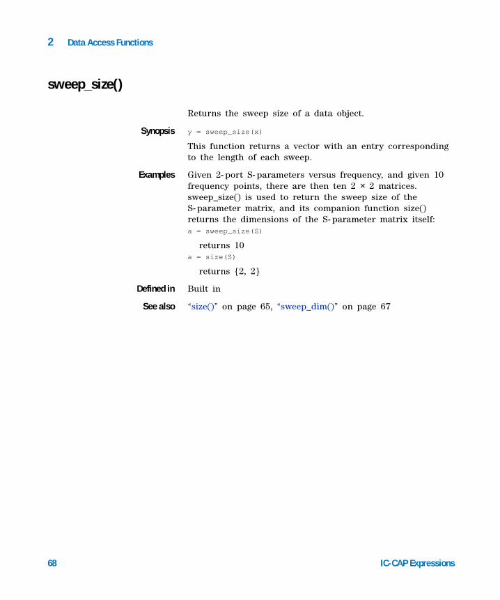
size() 65
sort() 66
sweep_dim() 67
sweep_size() 68
type() 69
vs() 70
what() 71

IC-CAP Expressions 5
write_var() 72
3 Harmonic Balance Functions
Working with Harmonic Balance Data 76
carr_to_im() 77
cdrange() 78
dc_to_rf() 79
ifc() 80
ip3_in() 81
ip3_out() 82
ipn() 83
it() 84
mix() 85
pae() 86
pfc() 87
phase_gain() 88
pspec() 89
pt() 90
remove_noise() 91
sfdr() 92
snr() 94
spur_track() 95
spur_track_with_if() 97
thd_func() 99
ts() 100
6 IC-CAP Expressions
vfc() 102
vspec() 103
vt() 104
4 Math Functions
abs() 108
acos() 109
acosh() 110
acot() 111
acoth() 112
asin() 113
asinh() 114
atan() 115
atan2() 116
atanh() 117
ceil() 118
cint() 119
cmplx() 120
complex() 121
conj() 122
convBin() 123
convHex() 124
convInt() 125
convOct() 126
cos() 127

IC-CAP Expressions 7
cosh() 128
cot() 129
coth() 130
cum_prod() 131
cum_sum() 132
db() 133
dbm() 134
dbmtow() 136
deg() 137
diagonal() 138
diff() 139
erf() 140
erfc() 141
erfcinv() 142
erfinv() 143
exp() 144
fft() 145
fix() 146
float() 147
floor() 148
fmod() 149
hypot() 150
identity() 151
im() 152
imag() 153
8 IC-CAP Expressions
int() 154
integrate() 155
interp() 156
interpolate() 157
inverse() 158
jn() 159
ln() 160
log() 161
log10() 162
mag() 163
max() 164
max_outer() 165
max2() 166
mean() 167
mean_outer() 168
median() 169
min() 170
min_outer() 171
min2() 172
num() 173
ones() 174
phase() 175
phase_comp() 176
phasedeg() 177
phaserad() 178

IC-CAP Expressions 9
polar() 179
pow() 180
prod() 181
rad() 182
re() 183
real() 184
rms() 185
round() 186
sgn() 187
sin() 188
sinc() 189
sinh() 190
sqr() 191
sqrt() 192
sum() 193
tan() 194
tanh() 195
transpose() 196
unwrap() 197
wtodbm() 198
xor() 199
zeros() 200
5 S-parameter Analysis Functions
abcdtoh() 203

10 IC-CAP Expressions
abcdtos() 204
abcdtoy() 205
abcdtoz() 206
bandwidth_func() 207
center_freq() 208
dev_lin_phase() 209
ga_circle() 210
gain_comp() 212
gl_circle() 213
gp_circle() 215
gs_circle() 217
htoabcd() 219
htos() 220
htoy() 221
htoz() 222
ispec() 223
l_stab_circle() 224
l_stab_circle_center_radius() 225
l_stab_region() 226
map1_circle() 227
map2_circle() 228
max_gain() 229
mu() 230
mu_prime() 231
ns_circle() 232
IC-CAP Expressions 11
ns_pwr_int() 234
ns_pwr_ref_bw() 235
pwr_gain() 236
ripple() 237
s_stab_circle() 238
s_stab_circle_center_radius() 239
s_stab_region() 240
sm_gamma1() 241
sm_gamma2() 242
sm_y1() 243
sm_y2() 244
sm_z1() 245
sm_z2() 246
stab_fact() 247
stab_meas() 248
stoabcd() 249
stoh() 250
stos() 251
stot() 252
stoy() 253
stoz() 254
tdr_sp_gamma() 255
tdr_sp_imped() 256
tdr_step_imped() 257
ttos() 258

12 IC-CAP Expressions
unilateral_figure() 259
volt_gain() 261
volt_gain_max() 263
vswr() 264
write_snp() 265
yin() 267
yopt() 268
ytoabcd() 269
ytoh() 270
ytos() 271
ytoz() 272
zin() 273
zopt() 274
ztoabcd() 275
ztoh() 276
ztos() 277
ztoy() 278
6 Statistical Analysis Functions
cdf() 280
cross_corr() 281
histogram() 282
histogram_multiDim() 284
histogram_sens() 285
histogram_stat() 286

IC-CAP Expressions 13
lognorm_dist_inv1D() 287
lognorm_dist1D() 288
moving_average() 289
norm_dist_inv1D() 290
norm_dist1D() 291
norms_dist_inv1D() 292
norms_dist1D() 293
pdf() 294
stddev() 295
stddev_outer() 296
uniform_dist_inv1D() 297
uniform_dist1D() 298
yield_sens() 299
7 Transient Analysis Functions
Working with Transient Data 302
constellation() 303
cross() 305
fspot() 306
ifc_tran() 309
ispec_tran() 310
pfc_tran() 311
pspec_tran() 312
pt_tran() 313
step() 314

14 IC-CAP Expressions
vfc_tran() 315
vspec_tran() 316
vt_tran() 317

15
Agilent 85190A IC-CAP 2006Expressions
Agilent Technologies
1Introduction to Measurement Expressions
Measurement Expressions Syntax 19
Manipulating IC-CAP Data with Expressions 24
User-Defined Functions 28
Functions Reference Format 30
Alphabetical Listing of Measurement Expressions 31
This document describes the measurement expressions that are available for use with IC- CAP. For a complete list of available measurement expressions, refer to the “Alphabetical Listing of Measurement Expressions” on page 31 or consult the index.
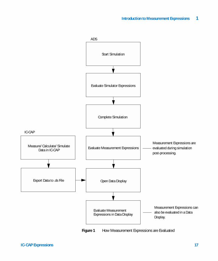
Measurement expressions are equations that are evaluated during post processing. They can be entered into the program using various methods, depending on which product you are using. In ADS, measurement expressions are evaluated during simulation post- processing and can also be evaluated in the Data Display. In IC- CAP, measurement expressions can only be evaluated in the Data Display. For more information on entering equations in a data display, refer to the Data Display documentation.
NOTE Measurement expressions are based on the mathematical syntax in Application Extension Language (AEL) and are NOT usable in IC-CAP’s Parameter Extraction Language (PEL).

16 IC-CAP Expressions
1 Introduction to Measurement Expressions
The following figure illustrates the differences between IC- CAP and ADS in evaluating measurement expressions.
Introduction to Measurement Expressions 1
IC-CAP Expressions 17
Figure 1 How Measurement Expressions are Evaluated
Measurement Expressions are
evaluated during simulation
post-processing.
Measurement Expressions canalso be evaluated in a DataDisplay.
Start Simulation
Evaluate Simulator Expressions
Complete Simulation
Evaluate Measurement Expressions
Open Data Display
Evaluate Measurement Expressions in Data Display
Measure/Calculate/Simulate Data in IC-CAP
Export Data to .ds File
IC-CAP
ADS
18 IC-CAP Expressions
1 Introduction to Measurement Expressions
Within this document you will find information on:
• “Measurement Expressions Syntax” on page 19
• “Manipulating IC- CAP Data with Expressions” on page 24
• Information on working with different types of data.
• Information specific to entering simulator expressions in your particular product.
You will also find a complete list of functions that can be used as measurement expressions individually, or combined together as a nested expression. These expressions have been separated into libraries and are listed in alphabetical order within each library. The expressions available include:
• Chapter 2, “Data Access Functions
• Chapter 3, “Harmonic Balance Functions
• Chapter 4, “Math Functions
• Chapter 5, “S- parameter Analysis Functions
• Chapter 6, “Statistical Analysis Functions
• Chapter 7, “Transient Analysis Functions
For a complete listing of all functions provided in this document, refer to “Alphabetical Listing of Measurement Expressions” on page 31 or consult the index.
Introduction to Measurement Expressions 1
IC-CAP Expressions 19
Measurement Expressions Syntax
Use the following guidelines when creating measurement expressions:
• Measurement expressions are based on the mathematical syntax in Application Extension Language (AEL).
• Function names, variable names and constant names are all case sensitive in measurement expressions.
• Use commas to separate arguments.
• White space between arguments is acceptable.
Case Sensitivity
All variable names, functions names, and equation names are case sensitive in measurement expressions.
Variable Names
Data produced by IC- CAP can be referenced in equations with various degrees of rigidity. IC- CAP output and transform names are referred to as variables in the Data Display window. In general, a Data Display variable is defined as:
DatasetName.Model.DUT.Setup.<KEY>.<DataType>.Name
where
<KEY> is either XFORM or ICCAP_SWEPT_DATA. Data under ICCAP_SWEPT_DATA are transforms or outputs that have the same number of points as specified by the inputs in the setup. Data under XFORM are transforms that have a different number of points than specified by the inputs in the setup.
<DataType> is either XFORM, SWEEP, or OUT. Data under XFORM is from transforms, under SWEEP is from inputs, and under OUT is from outputs.
By default, in the Data Display window, a variable is commonly referenced as:

20 IC-CAP Expressions
1 Introduction to Measurement Expressions
DatasetName..VariableName
where the double dot “..” indicates that the variable is unique in this dataset. If a variable is referenced without a dataset name, then it is assumed to be in the current default dataset.
When the results of several setups are in a dataset (very common when saving your entire .mdl to a .ds file), it becomes necessary to specify the setup and possibly the DUT name with the variable name. This is only necessary when a particular output name (id, ia, etc.) is used in multiple setups. The double dot can always be used to pad a variable name instead of specifying the complete name.
The most common use of the double dot is when it is desired to tie a variable to a dataset other than the default dataset.
Built-in Constants
The following constants can be used in measurement expressions.
NOTE If a dataset has a single output of type measured or simulated, the measured output is named m and the simulated output is named s. If a dataset has at least two measured or simulated outputs, the outputs are given more readable names such as id.m and id.s.
Table 1 Built-in Constants
Constant Description Value
PI (also pi) π 3.1415926535898
e Euler’s constant 2.718281822
ln10 natural log of 10 2.302585093
boltzmann Boltzmann’s constant 1.380658e–23 J/K
qelectron electron charge 1.60217733e–19 C
planck Planck’s constant 6.6260755e-34 J*s

Introduction to Measurement Expressions 1
IC-CAP Expressions 21
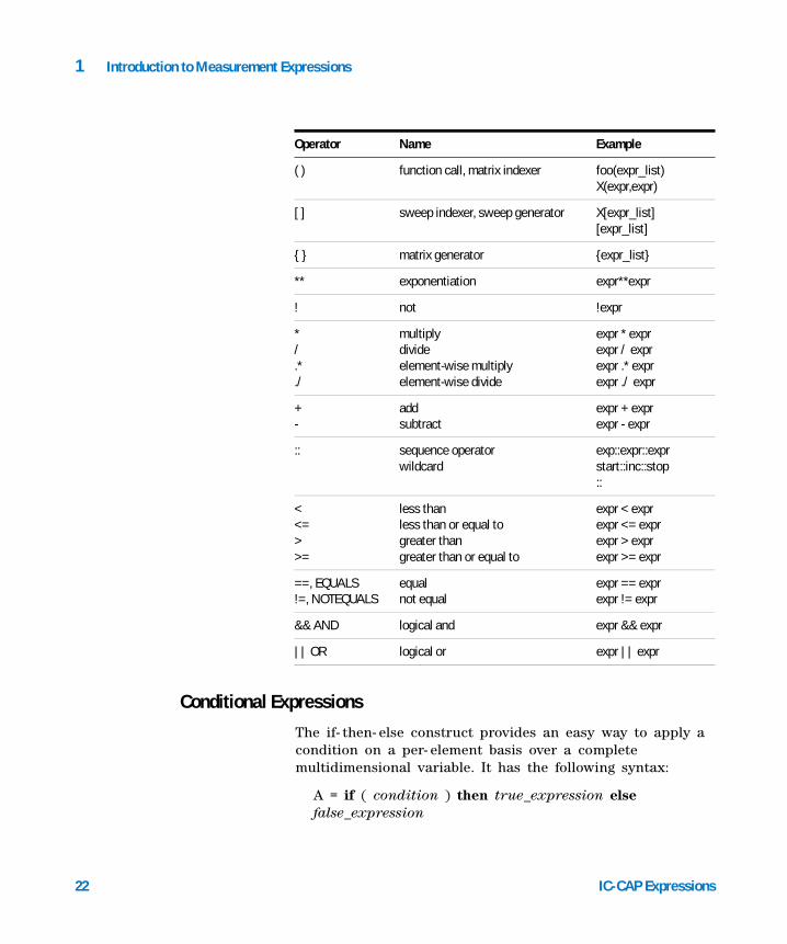
Operator Precedence
Measurement expressions are evaluated from left to right, unless there are parentheses. Operators are listed from higher to lower precedence. Operators on the same line have the same precedence. For example, a+b*c means a+(b*c), because * has a higher precedence than +. Similarly, a+b- c means (a+b)–c, because + and – have the same precedence (and because + is left- associative).
The operators !, &&, and || work with the logical values. The operands are tested for the values TRUE and FALSE, and the result of the operation is either TRUE or FALSE. In AEL a logical test of a value is TRUE for non- zero numbers or strings with non- zero length, and FALSE for 0.0 (real), 0 (integer), NULL or empty strings. Note that the right hand operand of && is only evaluated if the left hand operand tests TRUE, and the right hand operand of || is only evaluated if the left hand operand tests FALSE.
The operators >=, <=, >, <, ==, != , AND, OR, EQUALS, and NOT EQUALS also produce logical results, producing a logical TRUE or FALSE upon comparing the values of two expressions. These operators are most often used to compare two real numbers or integers. These operators operate differently in AEL than C with string expressions in that they actually perform the equivalent of strcmp() between the first and second operands, and test the return value against 0 using the specified operator.
c0 Speed of light in free space 2.99792e+08 m/s
e0 Permittivity of free space 8.85419e–12 F/m
u0 Permeability of free space 12.5664e–07 H/m
i, j sqrt(–1) 1i
Table 1 Built-in Constants
Constant Description Value
22 IC-CAP Expressions
1 Introduction to Measurement Expressions
Conditional Expressions
The if- then- else construct provides an easy way to apply a condition on a per- element basis over a complete multidimensional variable. It has the following syntax:
A = if ( condition ) then true_expression else false_expression
Operator Name Example
( ) function call, matrix indexer foo(expr_list)X(expr,expr)
[ ] sweep indexer, sweep generator X[expr_list][expr_list]
{ } matrix generator {expr_list}
** exponentiation expr**expr
! not !expr
* / .*./
multiplydivideelement-wise multiply element-wise divide
expr * exprexpr / exprexpr .* exprexpr ./ expr
+-
addsubtract
expr + exprexpr - expr
:: sequence operatorwildcard
exp::expr::exprstart::inc::stop::
< <= >>=
less thanless than or equal to greater thangreater than or equal to
expr < exprexpr <= exprexpr > exprexpr >= expr
==, EQUALS!=, NOTEQUALS
equalnot equal
expr == exprexpr != expr
&& AND logical and expr && expr
|| OR logical or expr || expr

Introduction to Measurement Expressions 1
IC-CAP Expressions 23
Condition, true_expression, and false_expression are any valid expressions. The dimensionality and number of points in these expressions follow the same matching conditions required for the basic operators.
Multiple nested if- then- else constructs can also be used:
A = if ( condition ) then true_expression elseif ( condition2) then true_expression else false_expression
The type of the result depends on the type of the true and false expressions. The size of the result depends on the size of the condition, the true expression, and the false expression.

24 IC-CAP Expressions
1 Introduction to Measurement Expressions
Manipulating IC-CAP Data with Expressions
Expressions defined in this documentation are designed to manipulate data produced by IC- CAP. Expressions may reference any IC- CAP data, and may be placed in a Data Display window.
IC-CAP Data
The expressions package has inherent support for two main IC- CAP data features. First, IC- CAP data are normally multidimensional. Each sweep introduces a dimension. All operators and relevant functions are designed to apply themselves automatically over a multidimensional IC- CAP output. Second, the independent (swept) variable is associated with the data (for example, S- parameter data). This independent is propagated through expressions, so that the results of equations are automatically plotted or listed against the relevant swept variable.
Generating Data
Datasets exported from IC- CAP contain scalars and matrices. When a sweep is being performed, the sweep can produce scalars and matrices as a function of a set of swept variables. It is also possible to generate data by using expressions. Two operators can be used to do this. The first is the sweep generator “[ ]”, and the second is the matrix generator “{ }”. These operators can be combined in various ways to produce swept scalars and matrices. The data can then be used in the normal way in other expressions. The operators can also be used to concatenate existing data, which can be very useful when combined with the indexing operators.
In the Data Display, you can also create an array from an equation by combining two or more equations in the following manner:

Introduction to Measurement Expressions 1
IC-CAP Expressions 25
A=2B=3C=[A,B]
Simple Sweeps and Using “[ ]”
Data from an IC- CAP setup generally contains at least one sweep. For a DC setup, this may be a bias sweep. For a two port analysis, your primary sweep may be frequency. IC- CAP generates this data in a .ds file such that outputs and transforms with this data shape are attached to this sweep information. This association is visible from the hierarchy of the variables listed under any ICCAP_SWEPT_DATA branch in your dataset.
Often with a setup that contains multidimensional data, we want to look at a single sweep point or group of points. The sweep indexer “[ ]” can be used to do this. The sweep indexer is zero offset, meaning that the first sweep point is accessed as index 0. A sweep of n points can be accessed by means of an index that runs from 0 to n–1. Also, the what() function can be useful in indexing sweeps. Use what() to find out how many sweep points there are, and then use an appropriate index. Indexing out of range yields an invalid result.
The sequence operator can also be used to index into a subsection of a sweep. Given a parameter X, a subsection of X may be indexed as
a=X[start::increment::stop]
Because increment defaults to one,
a=X[start::stop]
is equivalent to
a=X[start::1::stop]
The “::” operator alone is the wildcard operator, so that X and X[::] are equivalent. Indexing can similarly be applied to multidimensional data. As will be shown later, an index may be applied in each dimension.

26 IC-CAP Expressions
1 Introduction to Measurement Expressions
S-parameters and Matrices
As previously described, the sweep indexer “[ ]” is used to index into a sweep. However, IC- CAP can produce a swept matrix, as when an S- parameter analysis is performed over some frequency range. Matrix entries can be referenced as S11 through Snm. While this is sufficient for most simple applications, it is also possible to index matrices by using the matrix indexer “()”. For example, S(1,1) is equivalent to S11. The matrix indexer is offset by one meaning the first matrix entry is X(1,1). When it is used with swept data its operation is transparent with respect to the sweep. Both indexers can be combined. For example, it is possible to access S(1,1) at the first sweep point as S(1,1)[0]. As with the sweep indexer “[ ]”, the matrix indexer can be used with wild cards and sequences to extract a submatrix from an original matrix.
Matrices
S- parameters above are an example of a matrix produced when a Two Port output or a transform with matrix data is exported to a dataset. Mathematical operators implement matrix operations. Element- by- element operations can be performed by using the dot modified operators (.* and ./).
The matrix indexer conveniently operates over the complete sweep, just as the sweep indexer operates on all matrices in a sweep. As with scalars, the mathematical operators allow swept and non- swept quantities to be combined. For example, the first matrix in a sweep may be subtracted from all matrices in that sweep as
Y = X- X[0]
Introduction to Measurement Expressions 1
IC-CAP Expressions 27
Multidimensional Sweeps and Indexing
In the previous examples we looked at single- dimensional sweeps. Multidimensional sweeps are very common in Two- Port setups with an outer bias sweep and in DC characteristics with multiple bias sweeps. Expressions are designed to operate on the multidimensional data. Functions and operators behave in a meaningful way when a parameter sweep is added or taken away. A common example is DC IV characteristics.
The sweep indexer accepts a list of indices. Up to N indices are used to index N- dimensional data. If fewer than N lookup indices are used with the sweep indexer, then wild cards are inserted automatically to the left.
28 IC-CAP Expressions
1 Introduction to Measurement Expressions
User-Defined Functions
By writing some Application Extension Language (AEL) code, you can define your own custom functions. The following file is provided specifically for this purpose:
$ICCAP_ROOT/expressions/ael/user_defined_fun.ael
By reviewing the other _fun.ael files in this directory, you can see how to write your own code. You can have as many functions as you like in this one file, and they will all be compiled upon program start- up. If you have a large number of functions to define, you may want to organize them into more than one file. In this case, include a line such as:
load("more_user_defined_fun.ael");
These load statements are added to the user_defined_fun.ael in the same directory in order to have your functions all compile. To create your own custom user defined functions:
1 Copy the $ICCAP_ROOT/expressions/ael/user_defined_fun.ael file to one of the following directories.
$HOME/hpeesof/expressions/ael (User Config)
$ICCAP_ROOT/custom/expressions/ael (Site Config)
Create the appropriate subdirectories if they do not already exist. The User Config is setup for a single user. The Site Config can be set up by a CAD Manager or librarian to control a site configuration for a group of users.
2 Edit the new file and add any custom defined functions. If your custom functions reside in another file, you can add a load statement to your new user_defined_fun.ael file to include your functions in another file. For example:
load("my_custom_functions_file.ael");
3 Save your changes to the new file and restart so your changes take effect. The search path looks in the following locations for user defined functions.

Introduction to Measurement Expressions 1
IC-CAP Expressions 29
$HOME/hpeesof/expressions/ael (Config)
$ICCAP_ROOT/custom/expressions/ael (Site Config)
$ICCAP_ROOT/expressions/ael (Default Config)
NOTE If for some reason your functions are not recognized, check to ensure that the user_defined_fun.atf (compiled version of user_defined_fun.ael file) was generated after restarting the software.

30 IC-CAP Expressions
1 Introduction to Measurement Expressions
Functions Reference Format
The information below illustrates how each measurement expression in the functions reference is described.
<function name> Presents a brief description of what the function does.
Synopsis Presents the general syntax of the function, including a description of the arguments.
Examples Presents one or more simple examples that use the function.
Defined in Indicates whether the measurement function is defined in a script or is built in. All AEL functions are built in.
See also Lists related functions, if any.
Notes/Equations Describes any additional notes and equations.
NOTE Optional arguments described in the Synopsis section are enclosed with curly braces. For example, y = ga_circle(S{, gain, numOfPts, numCircles, gainStep}), where gain, numOfPts, numCircles, and gainStep are all optional arguments. This should not be confused with the required syntax or the use of braces in the matrix generator described in “Generating Data” on page 24.
Introduction to Measurement Expressions 1
IC-CAP Expressions 31
Alphabetical Listing of Measurement Expressions
A“abcdtoh()” on page 203“abcdtos()” on page 204“abcdtoy()” on page 205“abcdtoz()” on page 206“abs()” on page 108“acos()” on page 109“acosh()” on page 110
“acot()” on page 111“acoth()” on page 112“asin()” on page 113“asinh()” on page 114“atan()” on page 115“atan2()” on page 116“atanh()” on page 117
B“bandwidth_func()” on page 207
“build_subrange()” on page 39
C“carr_to_im()” on page 77“cdf()” on page 280“cdrange()” on page 78“ceil()” on page 118“center_freq()” on page 208“chop()” on page 40“chr()” on page 41“cint()” on page 119“circle()” on page 42“cmplx()” on page 120“collapse()” on page 43“complex()” on page 121“conj()” on page 122“constellation()” on page 303“contour()” on page 44
“contour_polar()” on page 46“convBin()” on page 123“convHex()” on page 124“convInt()” on page 125“convOct()” on page 126“copy()” on page 47“cos()” on page 127“cosh()” on page 128“cot()” on page 129“coth()” on page 130“create()” on page 48“cross()” on page 305“cross_corr()” on page 281“cum_prod()” on page 131“cum_sum()” on page 132
D“db()” on page 133“dbm()” on page 134“dbmtow()” on page 136“dc_to_rf()” on page 79“deg()” on page 137
“delete()” on page 51“dev_lin_phase()” on page 209“diagonal()” on page 138“diff()” on page 139
32 IC-CAP Expressions
1 Introduction to Measurement Expressions
E“erf()” on page 140“erfc()” on page 141“erfcinv()” on page 142
“erfinv()” on page 143“exp()” on page 144“expand()” on page 52
F“fft()” on page 145“find()” on page 53“find_index()” on page 54“fix()” on page 146“float()” on page 147
“floor()” on page 148“fmod()” on page 149“fspot()” on page 306“fun_2d_outer()” on page 55
G“ga_circle()” on page 210“gain_comp()” on page 212“generate()” on page 56“get_attr()” on page 57
“get_indep_values()” on page 58“gl_circle()” on page 213“gp_circle()” on page 215“gs_circle()” on page 217
H“histogram()” on page 282“histogram_multiDim()” on page 284“histogram_sens()” on page 285“histogram_stat()” on page 286
“htoabcd()” on page 219“htos()” on page 220“htoy()” on page 221“hypot()” on page 150
I“identity()” on page 151“ifc()” on page 80“ifc_tran()” on page 309“im()” on page 152“imag()” on page 153“indep()” on page 59“int()” on page 154“integrate()” on page 155
“interp()” on page 156“interpolate()” on page 157“inverse()” on page 158“ip3_in()” on page 81“ip3_out()” on page 82“ipn()” on page 83“ispec()” on page 223“ispec_tran()” on page 310“it()” on page 84
J“jn()” on page 159

Introduction to Measurement Expressions 1
IC-CAP Expressions 33
L“l_stab_circle()” on page 224“l_stab_circle_center_radius()” on page 225“l_stab_region()” on page 226“ln()” on page 160
“log()” on page 161“log10()” on page 162“lognorm_dist_inv1D()” on page 287“lognorm_dist1D()” on page 288
M“mag()” on page 163“map1_circle()” on page 227“map2_circle()” on page 228“max()” on page 164“max_gain()” on page 229“max_index()” on page 60“max_outer()” on page 165“max2()” on page 166“mean()” on page 167“mean_outer()” on page 168
“median()” on page 169“min()” on page 170“min_index()” on page 61“min_outer()” on page 171“min2()” on page 172“mix()” on page 85“moving_average()” on page 289“mu()” on page 230“mu_prime()” on page 231
N“norm_dist_inv1D()” on page 290“norm_dist1D()” on page 291“norms_dist_inv1D()” on page 292“norms_dist1D()” on page 293
“ns_circle()” on page 232“ns_pwr_int()” on page 234“ns_pwr_ref_bw()” on page 235“num()” on page 173
O“ones()” on page 174
P“pae()” on page 86“pdf()” on page 294“permute()” on page 62“pfc()” on page 87“pfc_tran()” on page 311“phase()” on page 175“phase_comp()” on page 176“phasedeg()” on page 177“phase_gain()” on page 88
“phaserad()” on page 178“plot_vs()” on page 63“polar()” on page 179“pow()” on page 180“prod()” on page 181“pspec()” on page 89“pspec_tran()” on page 312“pt_tran()” on page 313“pt()” on page 90“pwr_gain()” on page 236
34 IC-CAP Expressions
1 Introduction to Measurement Expressions
R“rad()” on page 182“re()” on page 183“real()” on page 184“remove_noise()” on page 91
“ripple()” on page 237“rms()” on page 185“round()” on page 186
S“s_stab_circle()” on page 238“s_stab_circle_center_radius()” on page 239“s_stab_region()” on page 240“set_attr()” on page 64“sfdr()” on page 92“sgn()” on page 187“sin()” on page 188“sinc()” on page 189“sinh()” on page 190“size()” on page 65“sm_gamma1()” on page 241“sm_gamma2()” on page 242“sm_y1()” on page 243“sm_y2()” on page 244“sm_z1()” on page 245“sm_z2()” on page 246“snr()” on page 94“sort()” on page 66
“spur_track()” on page 95“spur_track_with_if()” on page 97“sqr()” on page 191“sqrt()” on page 192“stab_fact()” on page 247“stab_meas()” on page 248“stddev()” on page 295“stddev_outer()” on page 296“step()” on page 314“stoabcd()” on page 249“stoh()” on page 250“stos()” on page 251“stot()” on page 252“stoy()” on page 253“stoz()” on page 254“sum()” on page 193“sweep_dim()” on page 67“sweep_size()” on page 68
T“tan()” on page 194“tanh()” on page 195“tdr_sp_gamma()” on page 255“tdr_sp_imped()” on page 256“tdr_step_imped()” on page 257“thd_func()” on page 99
“transpose()” on page 196“ts()” on page 100“ttos()” on page 258“type()” on page 69
U“uniform_dist_inv1D()” on page 297“uniform_dist1D()” on page 298
“unilateral_figure()” on page 259“unwrap()” on page 197
Introduction to Measurement Expressions 1
IC-CAP Expressions 35
V“vfc()” on page 102“vfc_tran()” on page 315“volt_gain()” on page 261“volt_gain_max()” on page 263“vs()” on page 70
“vspec_tran()” on page 316“vspec()” on page 103“vswr()” on page 264“vt()” on page 104“vt_tran()” on page 317
W“what()” on page 71“write_snp()” on page 265
“write_var()” on page 72“wtodbm()” on page 198
X“xor()” on page 199
Y“yield_sens()” on page 299“yin()” on page 267“yopt()” on page 268“ytoabcd()” on page 269
“ytoh()” on page 270“ytos()” on page 271“ytos()” on page 271“ytoz()” on page 272
Z“zeros()” on page 200“zin()” on page 273“zopt()” on page 274“ztoabcd()” on page 275
“ztoh()” on page 276“ztos()” on page 277“ztoy()” on page 278

36 IC-CAP Expressions
1 Introduction to Measurement Expressions
37
Agilent 85190A IC-CAP 2006Expressions
Agilent Technologies
2Data Access Functions
build_subrange() 39
chop() 40
chr() 41
circle() 42
collapse() 43
contour() 44
contour_polar() 46
copy() 47
create() 48
delete() 51
expand() 52
find() 53
find_index() 54
fun_2d_outer() 55
generate() 56
get_attr() 57
get_indep_values() 58
indep() 59
max_index() 60
min_index() 61
permute() 62
plot_vs() 63
set_attr() 64
size() 65
sort() 66
sweep_dim() 67
sweep_size() 68
type() 69

38 IC-CAP Expressions
2 Data Access Functions
vs() 70
what() 71
write_var() 72
This chapter describes data access and data manipulation functions in detail. The functions are listed in alphabetical order.
NOTE You can use these functions to find information about a piece of data (e.g., independent values, size, type, attributes, etc.). You can also use some functions to generate data for plotting circles and contours.
Data Access Functions 2
IC-CAP Expressions 39
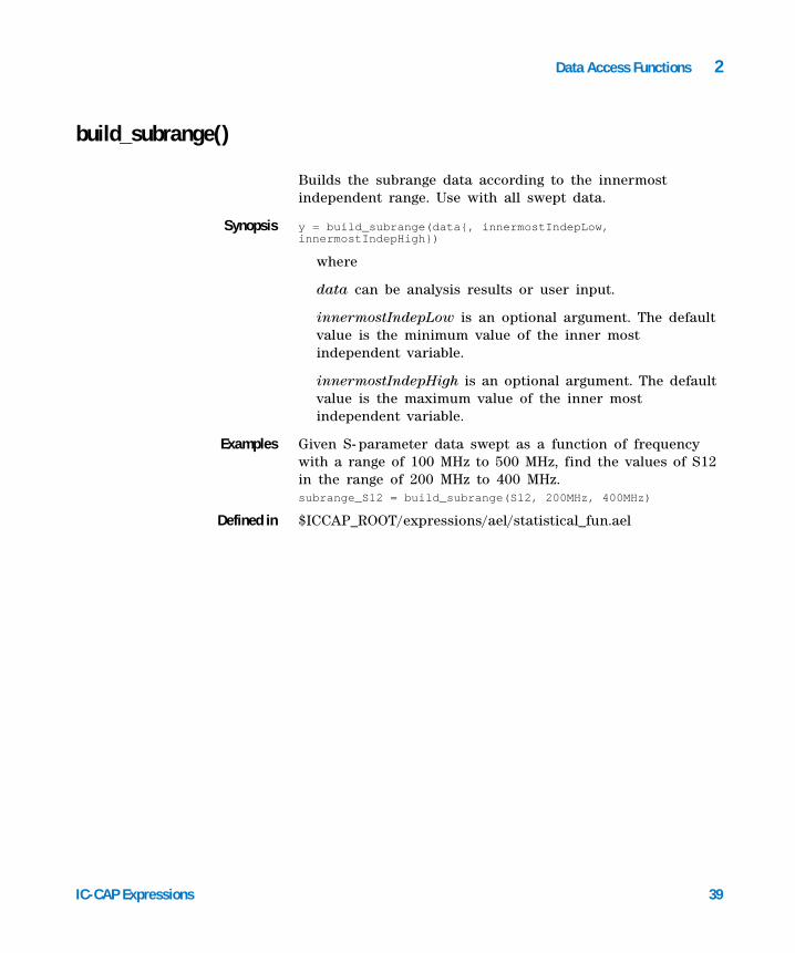
build_subrange()
Builds the subrange data according to the innermost independent range. Use with all swept data.
Synopsis y = build_subrange(data{, innermostIndepLow, innermostIndepHigh})
where
data can be analysis results or user input.
innermostIndepLow is an optional argument. The default value is the minimum value of the inner most independent variable.
innermostIndepHigh is an optional argument. The default value is the maximum value of the inner most independent variable.
Examples Given S- parameter data swept as a function of frequency with a range of 100 MHz to 500 MHz, find the values of S12 in the range of 200 MHz to 400 MHz.subrange_S12 = build_subrange(S12, 200MHz, 400MHz)
Defined in $ICCAP_ROOT/expressions/ael/statistical_fun.ael

40 IC-CAP Expressions
2 Data Access Functions
chop()
Replace numbers in x with magnitude less than dx with 0.
Synopsis y = chop(x{, dx})
then y= x if mag(x)>=mag(dx)
and y=0 if mag(x)<mag(dx)
dx is optional, default is 1e−10.
Actually this function is more complicated; it acts independently on the real and complex components of x, comparing each to mag(dx).
Examples chop(1)
returns 1chop(1e–12)
returns 0chop(1+1e–12i)
returns 1+0i
Defined in $ICCAP_ROOT/expressions/ael/elementary_fun.ael

Data Access Functions 2
IC-CAP Expressions 41
chr()
Returns the character representation of an integer.
Synopsis y = chr(x)
where x is a valid ASCII string representing a character.
Examples a = chr(64)
returns @
a = chr(60)
returns <a = chr(117)
returns u
Defined in Built in
42 IC-CAP Expressions
2 Data Access Functions
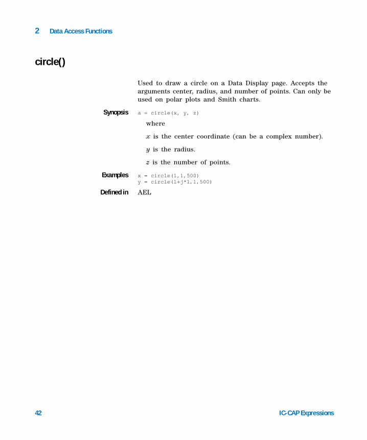
circle()
Used to draw a circle on a Data Display page. Accepts the arguments center, radius, and number of points. Can only be used on polar plots and Smith charts.
Synopsis a = circle(x, y, z)
where
x is the center coordinate (can be a complex number).
y is the radius.
z is the number of points.
Examples x = circle(1,1,500)y = circle(1+j*1,1,500)
Defined in AEL
Data Access Functions 2
IC-CAP Expressions 43
collapse()
Collapses the inner independent variable and returns one dimensional data.
Synopsis y = collapse(x)
where x is a required argument. Its dimension is larger than one and less than four.
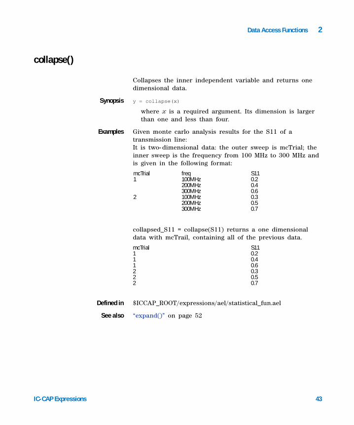
Examples Given monte carlo analysis results for the S11 of a transmission line: It is two- dimensional data: the outer sweep is mcTrial; the inner sweep is the frequency from 100 MHz to 300 MHz and is given in the following format:
collapsed_S11 = collapse(S11) returns a one dimensional data with mcTrail, containing all of the previous data.
Defined in $ICCAP_ROOT/expressions/ael/statistical_fun.ael
See also “expand()” on page 52
mcTrial freq S111 100MHz 0.2
200MHz 0.4300MHz 0.6
2 100MHz 0.3200MHz 0.5300MHz 0.7
mcTrial S111 0.21 0.41 0.62 0.32 0.52 0.7
44 IC-CAP Expressions
2 Data Access Functions
contour()
Generates contour levels on surface data.
Synopsis y = contour(data {, contour_levels, interpolatio_ type})
where
data is the data to be contoured, which must be at least two- dimensional real number or integer or implicit.
contour_levels is an optional one- dimensional quantity specifying the levels of the contours, which is normally specified by the sweep generator “[ ],” but can also be specified as a vector. If not provided, contour_levels defaults to six levels equally spaced between the maximum and the minimum of the data.
interpolation_type specifies the type of interpolation to perform. Types of interpolation supported are:
0 – No Interpolation (Default)
1 – Cubic Spline
2 – B- Spline
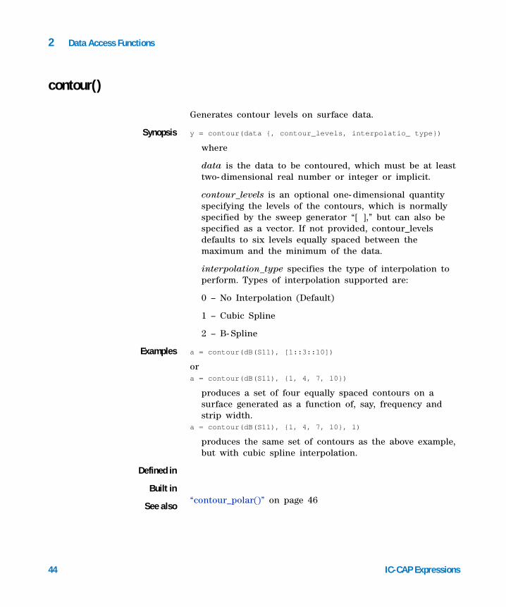
Examples a = contour(dB(S11), [1::3::10])
ora = contour(dB(S11), {1, 4, 7, 10})
produces a set of four equally spaced contours on a surface generated as a function of, say, frequency and strip width.
a = contour(dB(S11), {1, 4, 7, 10}, 1)
produces the same set of contours as the above example, but with cubic spline interpolation.
Defined in
Built in
See also“contour_polar()” on page 46
Data Access Functions 2
IC-CAP Expressions 45
Notes/Equations
This function introduces three extra inner independents into the data. The first two are "level", the contour level, and "number", the contour number. For each contour level there may be n contours. The contour is an integer running from 1 to n. The contour is represented as an (x, y) pair with x as the inner independent.
46 IC-CAP Expressions
2 Data Access Functions
contour_polar()
Generates contour levels on polar or Smith chart surface data.
Synopsis y = contour_polar(data {, contour_levels, interpolation_type})
where
data is the polar or Smith chart data to be contoured, (and therefore is surface data).
contour_levels is an optional one- dimensional quantity specifying the levels of the contours, which is normally specified by the sweep generator “[ ],” but can also be specified as a vector.
If not provided, contour_levels defaults to six levels equally spaced between the maximum and the minimum of the data.
interpolation_type specifies the type of interpolation to perform. Types of interpolation supported are:
0 - No Interpolation (Default)
1 - Cubic Spline
2 - B- Spline
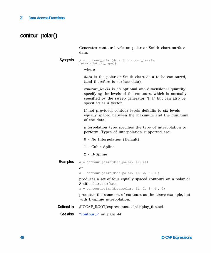
Examples a = contour_polar(data_polar, [1::4])
ora = contour_polar(data_polar, {1, 2, 3, 4})
produces a set of four equally spaced contours on a polar or Smith chart surface.a = contour_polar(data_polar, {1, 2, 3, 4}, 2)
produces the same set of contours as the above example, but with B- spline interpolation.
Defined in $ICCAP_ROOT/expressions/ael/display_fun.ael
See also “contour()” on page 44

Data Access Functions 2
IC-CAP Expressions 47
copy()
Makes a copy of a multi- dimensional data variable.
Synopsis y = copy(DataVar)
where DataVar is a data variable or array to be copied. The data type may be boolean, integer, real, complex, or string.
Examples result = copy(S21)
returns the copy of the data stored in the data variable S21.
The array or data variable created above can be used as follows:indepV = indep(result,"Index");result[0] = complex(1, 2); Sets the first value to a complex numberindepV[0] = 1GHz;
Defined in Built in
See also “create()” on page 48, “delete()” on page 51
Notes/Equations
Makes a copy of a multi- dimensional data variable, so that the contents of the copy can be manipulated. Data Variables are data structures that are used to hold multi- dimensional data. Internally they are not implemented as arrays, and therefore do not have the performance of an array. Accessing and setting data in these arrays are performance intensive and should be noted.

48 IC-CAP Expressions
2 Data Access Functions
create()
Creates a multi- dimensional data variable.
Synopsis y=create(Dimensionality, DependDataType, IndepName, IndepType, Numrows, Numcolumns)
where
Dimensionality is a required variable representing the dimensionality of the data variable or array. The variable must be an integer, with an allowed range of 1 to infinity.
DependDataType is an optional variable describing the dependent data type as either “Boolean“, “Integer”, “Real”, “Complex”, “String”, or “Byte16”. The variable must be a string. Default value is “Real”.
IndepNames is an optional variable describing the name(s) of independent. The variable must be a string. Default value is “__i”.
IndepType is an optional variable describing the independent data type as either “Boolean”, “Integer”, “Real”, “Complex”, “String”, or “Byte16”. The variable must be a string. Default value is “Real”.
NumRows is an optional variable representing the number of rows. The variable must be an integer with an allowed range of 0 to infinity. The default value is 0.
NumColumns is an optional variable representing the number of rows. The variable must be an integer with an allowed range of 0 to infinity. The default value is 0.
Examples result = create(1, "Complex", {"Index"}, {"Real"},1, 1);
returns a 1- dimensional data variable with dependent type Complex, independent name "Index" and type real with 1 row and column.
The array or data variable created above can be used as follows:indepV = indep(result,"Index");result[0] = 1.1;indepV[0] = 1.0;
Data Access Functions 2
IC-CAP Expressions 49
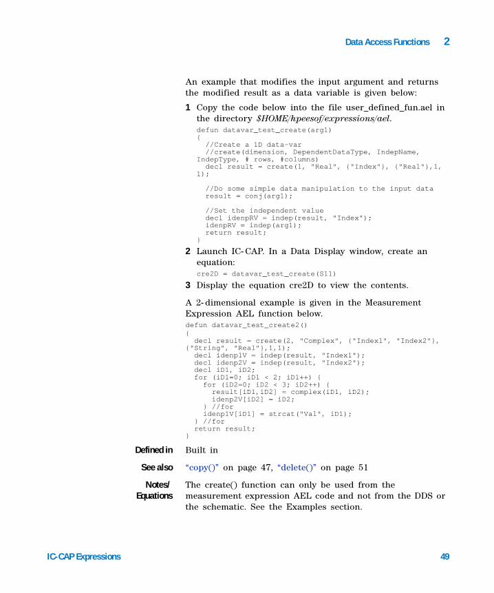
An example that modifies the input argument and returns the modified result as a data variable is given below:
1 Copy the code below into the file user_defined_fun.ael in the directory $HOME/hpeesof/expressions/ael. defun datavar_test_create(arg1){
//Create a 1D data-var//create(dimension, DependentDataType, IndepName,
IndepType, # rows, #columns)decl result = create(1, "Real", {"Index"}, {"Real"},1,
1);
//Do some simple data manipulation to the input dataresult = conj(arg1);
//Set the independent valuedecl idenpRV = indep(result, "Index");idenpRV = indep(arg1);return result;
}
2 Launch IC- CAP. In a Data Display window, create an equation: cre2D = datavar_test_create(S11)
3 Display the equation cre2D to view the contents.
A 2- dimensional example is given in the Measurement Expression AEL function below.defun datavar_test_create2(){
decl result = create(2, "Complex", {"Index1", "Index2"}, {"String", "Real"},1,1);
decl idenp1V = indep(result, "Index1");decl idenp2V = indep(result, "Index2");decl iD1, iD2;for (iD1=0; iD1 < 2; iD1++) {
for (iD2=0; iD2 < 3; iD2++) {result[iD1,iD2] = complex(iD1, iD2);idenp2V[iD2] = iD2;
} //foridenp1V[iD1] = strcat("Val", iD1);
} //forreturn result;
}
Defined in Built in
See also “copy()” on page 47, “delete()” on page 51
Notes/Equations
The create() function can only be used from the measurement expression AEL code and not from the DDS or the schematic. See the Examples section.

50 IC-CAP Expressions
2 Data Access Functions
This function is used to create multi- dimensional data variable or arrays. Data Variables in IC- CAP are data structures that are used to hold multi- dimensional data. Internally they are not implemented as arrays, and therefore do not have the performance of an array. Accessing and setting data in these arrays are performance intensive and should be noted.
The number of rows and columns are used in specifying the dimension of matrix data. For a scalar this would be 1, 1.
Data Access Functions 2
IC-CAP Expressions 51
delete()
Deletes the multi- dimensional data variable.
Synopsis y = delete(DataVar)
where DataVar is a data variable or array that is to be deleted. The data type may be boolean, integer, real, complex, or string.
Examples result = delete(S21)
returns true or false depending on whether the data variable was deleted or not.
Defined in Built in
See also “copy()” on page 47, “create()” on page 48

52 IC-CAP Expressions
2 Data Access Functions
expand()
Expands the dependent data of a variable into single points by introducing an additional inner independent variable.
Synopsis y = expand(x)
where x is a required argument. Its dimension is larger than one and less than four.
Examples Given a dependent data A which has independent variables B:
If A is a 1 dimensional data containing 4 points (10, 20, 30, and 40) and similarly B is made up of 4 points (1, 2, 3, and 4),Eqn A = [10,20,30,40]Eqn B = [1,2,3,4]Eqn C = vs(A,B,"X")
Using expand(C) increases the dimensionality of the data by 1 where each inner dependent variable ("X") consists of 1 point.Eqn Y = expand(C)
Defined in Built in
See also “collapse()” on page 43
X C A B Y
1234
10203040
10203040
1234
X=110
X=220
X=330
X=440
Data Access Functions 2
IC-CAP Expressions 53
find()
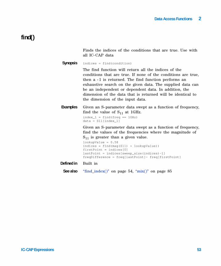
Finds the indices of the conditions that are true. Use with all IC- CAP data
Synopsis indices = find(condition)
The find function will return all the indices of the conditions that are true. If none of the conditions are true, then a - 1 is returned. The find function performs an exhaustive search on the given data. The supplied data can be an independent or dependent data. In addition, the dimension of the data that is returned will be identical to the dimension of the input data.
Examples Given an S- parameter data swept as a function of frequency, find the value of S11 at 1GHz.index_1 = find(freq == 1GHz)data = S11[index_1]
Given an S- parameter data swept as a function of frequency, find the values of the frequencies where the magnitude of S11 is greater than a given value.lookupValue = 0.58indices = find(mag(S11) > lookupValue))firstPoint = indices[0]lastPoint = indices[sweep_size(indices)-1]freqDifference = freq[lastPoint]- freq[firstPoint]
Defined in Built in
See also “find_index()” on page 54, “mix()” on page 85

54 IC-CAP Expressions
2 Data Access Functions
find_index()
Finds the closest index for a given search value. Use with all IC- CAP data.
Synopsis index = find_index(data_sweep, search_value)
To facilitate searching, the find_index function finds the index value in a sweep that is closest to the search value. Data of type int or real must be monotonic. find_index also performs an exhaustive search of complex and string data types.
Examples Given S- parameter data swept as a function of frequency, find the value of S11 at 1 GHz:index = find_index(freq, 1GHz)a = S11[index]
Defined in Built in
See also “find()” on page 53, “mix()” on page 85

Data Access Functions 2
IC-CAP Expressions 55
fun_2d_outer()
Applies a function to the outer dimension of two- dimensional data.
Synopsis y = fun_2d_outer(data, fun)
where
data must be two- dimensional data.
fun is some function (usually mean, max, or min) that will be applied to the outer dimension of the data.
Examples y = fun_2d_outer(data, min)
Defined in $ICCAP_ROOT/expressions/ael/statistcal_fun.ael
See also “max_outer()” on page 165, “mean_outer()” on page 168, “min_outer()” on page 171
Notes/Equations
Used in “max_outer()” on page 165, “mean_outer()” on page 168, “min_outer()” on page 171 functions.
Functions such as mean, max, and min operate on the inner dimension of two- dimensional data. The function fun_2d_outer enables these functions to be applied to the outer dimension. As an example, assume that a Monte Carlo simulation of an amplifier was run, with 151 random sets of parameter values, and that for each set the S- parameters were simulated over 26 different frequency points. S21 becomes a [151 Monte Carlo iteration X 26 frequency] matrix, with the inner dimension being frequency, and the outer dimension being Monte Carlo index. Now, assume that it is desired to know the mean value of the S- parameters at each frequency. Inserting an equation mean(S21) computes the mean value of S21 at each Monte Carlo iteration. If S21 is simulated from 1 to 26 GHz, it computes the mean value over this frequency range, which usually is not very useful. The function fun_2d_outer allows the mean to be computed over each element in the outer dimension.

56 IC-CAP Expressions
2 Data Access Functions
generate()
This function generates a sequence of real numbers. The modern way to do this is to use the sweep generator “[ ].”
Synopsis y = generate(start, stop, npts)
where
start is the first number.
stop is the last number.
npts is the number of numbers in the sequence.
Examples a = generate(9, 4, 6)
returns the sequence 9., 8., 7., 6., 5., 4.
Defined in Built in
Data Access Functions 2
IC-CAP Expressions 57
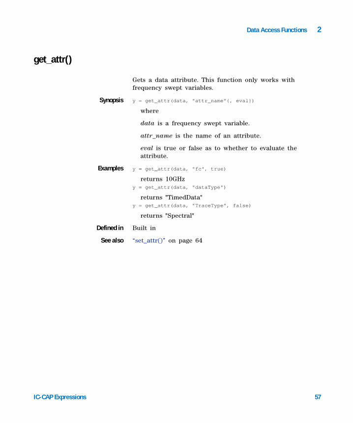
get_attr()
Gets a data attribute. This function only works with frequency swept variables.
Synopsis y = get_attr(data, "attr_name"{, eval})
where
data is a frequency swept variable.
attr_name is the name of an attribute.
eval is true or false as to whether to evaluate the attribute.
Examples y = get_attr(data, "fc", true)
returns 10GHzy = get_attr(data, "dataType")
returns "TimedData"y = get_attr(data, "TraceType", false)
returns "Spectral"
Defined in Built in
See also “set_attr()” on page 64
58 IC-CAP Expressions
2 Data Access Functions
get_indep_values()
Returns the independent values associated with the given dependent value as an array.
Synopsis indepVals = get_indep_values(Data, LookupValue)
where
Data is a 1 to 5 dimensional array.
LookupValue is the dependent value for which the corresponding independent values have to be found.
Examples We assume that the data is 2- dimensional i.e. 2 independent variables created from a Harmonic Balance Analysis with Pout being the output data.indepVals = get_indep_values(Pout, max(max(Pout))
returns the values of the independent as an array
Defined in $HPEESOF_DIR/expressions/ael/utility_fun.ael
See also “indep()” on page 59
Notes/Equations
This function can be used only on 1 to 5 dimensional data. The independent values have to be real. The dependent value to be looked up can only be a single value.

Data Access Functions 2
IC-CAP Expressions 59
indep()
Returns the independent attached to the data
Synopsis Y = indep(x)Y = indep(x, dimension)Y = indep(x, "indep_name")
indep() returns the independent (normally the swept variable) attached to IC- CAP data. When there is more than one independent, then the independent of interest may be specified by number or by name. If no independent specifications are passed, then indep() returns the innermost independent.
Examples Given S- parameters versus frequency and power: Frequency is the innermost independent, so its index is 1. Power has index 2. freq = indep(S, 1)freq = indep(S, "freq")power = indep(S, 2)power = indep(S, "power")
Defined in Built in
See also “find_index()” on page 54

60 IC-CAP Expressions
2 Data Access Functions
max_index()
Returns the index of the maximum.
Synopsis y = max_index(x)
The function takes a single argument, so enclose a sequence of numbers in brackets “[a, b, c, ...]”
Examples y = max_index([1, 2, 3])
returns 2y = max_index([3, 2, 1])
returns 0
Defined in Built- in
See also “min_index()” on page 61

Data Access Functions 2
IC-CAP Expressions 61
min_index()
Returns the index of the minimum
Synopsis y = min_index(x)
The function takes a single argument, so enclose a sequence of numbers in brackets “[a, b, c, ...]”
Examples a = min_index([3, 2, 1])
returns 2a = min_index([1, 2, 3])
returns 0
Defined in Built in
See also “max_index()” on page 60

62 IC-CAP Expressions
2 Data Access Functions
permute()
Permutes data based on the attached independents.
Synopsis y = permute(data, permute_vector)
where
data is any N- dimensional square data (all inner independents must have the same value N).
permute_vector is any permutation vector of the numbers 1 through N. The permute_vector defaults to {N::1}, representing a complete reversal of the data with respect to its independent variables. If permute_vector has fewer than N entries, the remainder of the vector, representing the outer independent variables, is filled in. In this way, expressions remain robust when outer sweeps are added.
Examples a = permute(data)a = permute(data, {3, 2, 1})
reverses the (three inner independents of) the data.a = permute(data, {1, 2, 3})
preserves the data.
Defined in Built in

Data Access Functions 2
IC-CAP Expressions 63
plot_vs()
Attaches an independent to data for plotting.
Synopsis y = plot_vs(dependent, independent)
where
dependent is any N- dimensional square data (all inner independents must have the same value N).
independent is the independent variable.
Examples a=[1, 2, 3] b=[4, 5, 6]c=plot_vs(a, b)
Builds c with independent b, and dependent a.
Defined in $ICCAP_ROOT/expressions/ael/display_fun.ael
See also “indep()” on page 59, “vs()” on page 70
Notes/Equations
When using plot_vs(), the independent and dependent data should be the same size (i.e., not irregular).
64 IC-CAP Expressions
2 Data Access Functions
set_attr()
Sets the data attribute.
Synopsis y = set_attr(data, "attr_name", "attribute_value")
where
data is the data for which you want to set/change the attributes.
"attr_name" is the name of the attribute to be changed.
"attribute_value" is the value of the attribute to change to.
Examples a = set_attr(data, "TraceType", "Spectral")a = set_attr(data, "TraceType", "Histogram")
Defined in Built in
See also “get_attr()” on page 57
Data Access Functions 2
IC-CAP Expressions 65
size()
Returns the row and column size of a vector or matrix.
Synopsis Y = size(X)
Examples Given 2- port S- parameters versus frequency, and given 10 frequency points. Then for ten 2 × 2 matrices, size() returns the dimensions of the S- parameter matrix, and its companion function sweep_size() returns the size of the sweep:Y = size(S)
returns {2, 2}Y = sweep_size(S)
returns 10
Defined in Built in
See also “sweep_size()” on page 68

66 IC-CAP Expressions
2 Data Access Functions
sort()
This measurement returns a sorted variable in ascending or descending order. The sorting can be done on the independent or dependent variables. String values are sorted by folding them to lower case.
Synopsis y = sort(data, sortOrder, indepName)
where
data is a multidimensional scalar variable.
sortOrder is the sorting order, {"ascending", "descending"} (If not specified, it is set to "ascending").
indepName is used to specify the name of the independent variable for sorting (if not specified, the sorting is done on the dependent).
Examples a = sort(data) a = sort(data, "descending", "freq")
Defined in Built in
Data Access Functions 2
IC-CAP Expressions 67
sweep_dim()
Returns the dimensionality of the data.
Synopsis y = sweep_dim(x)
The function takes a single argument, so enclose a sequence of numbers in brackets “[a, b, c, ...]”
Examples a = sweep_dim(1)
returns 0a = sweep_dim([1, 2, 3])
returns 1
Defined in Built in
See also “sweep_size()” on page 68
68 IC-CAP Expressions
2 Data Access Functions
sweep_size()
Returns the sweep size of a data object.
Synopsis y = sweep_size(x)
This function returns a vector with an entry corresponding to the length of each sweep.
Examples Given 2- port S- parameters versus frequency, and given 10 frequency points, there are then ten 2 × 2 matrices. sweep_size() is used to return the sweep size of the S- parameter matrix, and its companion function size() returns the dimensions of the S- parameter matrix itself:a = sweep_size(S)
returns 10a = size(S)
returns {2, 2}
Defined in Built in
See also “size()” on page 65, “sweep_dim()” on page 67

Data Access Functions 2
IC-CAP Expressions 69
type()
Returns the type of the data.
Synopsis y = type(x)
Returns a string, which is one of “Integer”, “Real”, “Complex” or “String”
Examples a = type(1)
returns “Integer”a = type(1i)
returns “Complex”a = type(“type”)
returns “String”
Defined in Built in
See also “what()” on page 71
70 IC-CAP Expressions
2 Data Access Functions
vs()
Attaches an independent to data.
Synopsis y = vs(dependent, independent)
Examples a=[1, 2, 3] b=[4, 5, 6]c = vs(a, b)
Builds c with independent b, and dependent a.
Defined in Built in
See also “indep()” on page 59

Data Access Functions 2
IC-CAP Expressions 71
what()
Returns size and type of data. This function is used to determine the dimensions of a piece of data, the attached independents, the type, and (in the case of a matrix) the number of rows and columns. Use what() by entering a listing column and using the trace expression what(x).
Synopsis y = what(x)
Examples x=[10,20,30,40]
y=what(x)
Defined in Built in
See also “type()” on page 69
yDependency : [ ]Num. Points : [4]Matrix Size : scalarType : Integer

72 IC-CAP Expressions
2 Data Access Functions
write_var()
Writes dataset variables to a file.
Synopsis y=write_var(FileName, WriteMode, Comment, Delimiter, Format, Precision, Var1, Var2,...,VarN)
where
FileName is a required variable representing the name of the output file of the dataset variable. The variable must be a string.
WriteMode is a required variable that defines the write mode. The variable must be a string with a value of “W” for overwrite or “A” for append.
Comment is an optional variable that defines text to be written at the top of the file. The variable must be a string.
Delimiter is an optional variable that defines the delimiter that separates the data. The variable must be a string. The default value is “>”.
Format is an optional variable that defines the data format. The variable must be a string with a value of “f” for full notation or “s” for scientific notation. The default value is “f”.
Precision is an optional variable that defines the precision of the data. The variable must be a string with a value of [1,64]. The default value is 6.
Var1,...,VarN are data variables to be written. The variable must be a dataset variable.
Examples write_var_f=write_var("output_S21.txt","W","! Freq real(S21)imag(S21)"," ", "f", freq, S21)
writes S21 to the output file output_S21.txt as:! Freq real(S21) imag(S21)1000000000 0.60928892074273 -0.10958342264718 2000000000 0.52718867597783 -0.133191670023923000000000 0.4769067837712 -0.12080489345341
Data Access Functions 2
IC-CAP Expressions 73
Another example:wv_ib=write_var("output_hbIb.txt","W","! HB Ib.i", " ", "f", freq, Ib.i)
writes the Harmonic Balance frequency and current Ib.i to the output file output_hbIb.txt.
Defined in $HPEESOF_DIR/expressions/ael/utility_fun.ael
See also “indep()” on page 59
Notes/Equations
This function can be used to write multiple dataset variables to a file. Currently only 1- dimensional data is supported. All variables that are to be written must be of the same size. Each variable data is written in column format. Complex data type is written in 2 columns as real and imaginary.

74 IC-CAP Expressions
2 Data Access Functions

75
Agilent 85190A IC-CAP 2006Expressions
Agilent Technologies
3Harmonic Balance Functions
Working with Harmonic Balance Data 76
carr_to_im() 77
cdrange() 78
dc_to_rf() 79
ifc() 80
ip3_in() 81
ip3_out() 82
ipn() 83
it() 84
mix() 85
pae() 86
pfc() 87
phase_gain() 88
pspec() 89
pt() 90
remove_noise() 91
sfdr() 92
snr() 94
spur_track() 95
spur_track_with_if() 97
thd_func() 99
ts() 100
vfc() 102
vspec() 103
vt() 104
This chapter describes the harmonic balance functions in detail. The functions are listed in alphabetical order.

76 IC-CAP Expressions
3 Harmonic Balance Functions
Working with Harmonic Balance Data
Harmonic Balance (HB) Analysis produces complex voltages and currents as a function of frequency or harmonic number. A single analysis produces 1- dimensional data. Individual harmonic components can be indexed by means of “[ ]”. Multi- tone HB also produces 1- dimensional data. Individual harmonic components can be indexed as usual by means of “[ ]”. However, the function “mix()” on page 85 provides a convenient way to select a particular mixing component.
Harmonic Balance Functions 3
IC-CAP Expressions 77
carr_to_im()
This measurement gives the suppression (in dB) of a specified IMD product below the fundamental power at the output port.
Synopsis y = carr_to_im(vOut, fundFreq, imFreq{, Mix})
where
vOut is the signal voltage at the output port.
fundFreq and imFreq are the harmonic frequency indices for the fundamental frequency and IMD product of interest, respectively.
Mix is an optional argument. The mix variable consists of all possible vectors of harmonic frequency (mixing terms) in the analysis. It is required whenever the first argument is a spectrum obtained from an expression that operates on the voltage and/current spectrum.
Examples a = carr_to_im(out, {1, 0}, {2, –1})
Defined in $ICCAP_ROOT/expressions/ael/rf_system_fun.ael
See also “ip3_out()” on page 82

78 IC-CAP Expressions
3 Harmonic Balance Functions
cdrange()
Returns compression dynamic range.
Synopsis y = cdrange(nf, inpwr_lin, outpwr_lin, outpwr)
where
nf is noise figure at the output port.
inpwr_lin and outpwr_lin are input and the output power, respectively, in the linear region.
outpwr is output power at 1 dB compression.
Examples a = cdrange(nf2, inpwr_lin, outpwr_lin, outpwr)
Defined in $ICCAP_ROOT/expressions/ael/rf_system_fun.ael
See also “sfdr()” on page 92
Notes/Equations
Used in XDB simulation.
The compressive dynamic range ratio identifies the dynamic range from the noise floor to the 1- dB gain- compression point. The noise floor is the noise power with respect to the reference bandwidth.

Harmonic Balance Functions 3
IC-CAP Expressions 79
dc_to_rf()
This measurement computes the DC- to- RF efficiency of any part of the network.
Synopsis y = dc_to_rf(vPlusRF, vMinusRF, vPlusDC, vMinusDC, currentRF, currentDC, harm_freq_index{, Mix})
where
vPlusRF and vMinusRF are RF voltages at the negative terminals.
vPlusDC and vMinusDC are DC voltages at the negative terminals.
currentRF and currentDC are the RF and DC currents for power calculation.
harm_freq_index is harmonic index of the RF frequency at the output port.
Mix is an optional variable consisting of all possible vectors of harmonic frequency indices (mixing terms) in the analysis.
Examples a = dc_to_rf(vrf, 0, vDC, 0, I_Probe1.i, SRC1.i, {1,0})
Defined in $ICCAP_ROOT/expressions/ael/circuit_fun.ael
80 IC-CAP Expressions
3 Harmonic Balance Functions
ifc()
This measurement gives the RMS current value of one frequency- component of a harmonic balance waveform.
Synopsis y = ifc(iOut, harm_freq_index{, Mix})
where
iOut is the current through a branch.
harm_freq_index is the harmonic index of the desired frequency. Note that the harm_freq_index argument's entry should reflect the number of tones in the harmonic balance controller. For example, if one tone is used in the controller, there should be one number inside the braces; two tones would require two numbers separated by a comma.
Mix is an optional variable consisting of all possible vectors of harmonic frequency indices (mixing terms) in the analysis.
Examples The following example is for two tones in the harmonic balance controller:y = ifc(I_Probe1.i, {1, 0})
Defined in $ICCAP_ROOT/expressions/ael/circuit_fun.ael
See also “pfc()” on page 87, “vfc()” on page 102
Harmonic Balance Functions 3
IC-CAP Expressions 81
ip3_in()
This measurement determines the input third- order intercept point (in dBm) at the input port with reference to a system output port.
Synopsis y = ip3_in(vOut, ssGain, fundFreq, imFreq, zRef{, Mix})
where
vOut is the signal voltage at the output.
ssGain is the small signal gain in dB.
fundFreq and imFreq are the harmonic frequency indices for the fundamental and intermodulation frequencies, respectively.
zRef is the reference impedance.
Mix is an optional argument. The mix variable consists of all possible vectors of harmonic frequency (mixing terms) in the analysis. It is required whenever the first argument is a spectrum obtained from an expression that operates on the voltage and/current spectrum.
Examples y = ip3_in(vOut, 22, {1, 0}, {2, –1}, 50)
Defined in $ICCAP_ROOT/expressions/ael/rf_system_fun.ael
See also “ip3_out()” on page 82, “ipn()” on page 83
Notes/Equations
To measure the third- order intercept point, you must setup a Harmonic Balance simulation with the input signal driving the circuit in the linear range. Input power is typically set 10 dB below the 1 dB gain compression point. If you simulate the circuit in the nonlinear region, the calculated results will be incorrect.
82 IC-CAP Expressions
3 Harmonic Balance Functions
ip3_out()
This measurement determines the output third- order intercept point (in dBm) at the system output port.
Synopsis y = ip3_out(vOut, fundFreq, imFreq, zRef{, Mix})
where
vOut is the signal voltage at the output
fundFreq and imFreq are the harmonic frequency indices for the fundamental and intermodulation frequencies, respectively.
zRef is the reference impedance.
Mix is an optional argument. The mix variable consists of all possible vectors of harmonic frequency (mixing terms) in the analysis. It is required whenever the first argument is a spectrum obtained from an expression that operates on the voltage and/current spectrum.
Examples y = ip3_out(vOut, {1, 0}, {2, –1}, 50)
Defined in $ICCAP_ROOT/expressions/ael/rf_system_fun.ael
See also “ip3_in()” on page 81, “ipn()” on page 83
Notes/Equations
To measure the third- order intercept point, you must setup a Harmonic Balance simulation with the input signal driving the circuit in the linear range. Input power is typically set 10 dB below the 1 dB gain compression point. If you simulate the circuit in the nonlinear region, the calculated results will be incorrect.

Harmonic Balance Functions 3
IC-CAP Expressions 83
ipn()
This measurement determines the output nth- order intercept point (in dBm) at the system output port.
Synopsis y = ipn(vPlus, vMinus, iOut, fundFreq, imFreq, n)
where
vPlus and vMinus are the voltages at the positive and negative output terminals, respectively.
iOut is the current through a branch.
fundFreq and imFreq are the harmonic indices of the fundamental and intermodulation frequencies, respectively.
n is the order of the intercept.
Examples y = ipn(vOut, 0, I_Probe1.i, {1, 0}, {2, -1}, 3)
Defined in $ICCAP_ROOT/expressions/ael/circuit_fun.ael
See also “ip3_in()” on page 81, “ip3_out()” on page 82
Notes/Equations
To measure the third- order intercept point, you must setup a Harmonic Balance simulation with the input signal driving the circuit in the linear range. Input power is typically set 10 dB below the 1 dB gain compression point. If you simulate the circuit in the nonlinear region, the calculated results will be incorrect.

84 IC-CAP Expressions
3 Harmonic Balance Functions
it()
This measurement converts a harmonic- balance current frequency spectrum to a time- domain current waveform.
Synopsis it(iOut, tmin, tmax, numOfPnts)
where
iOut is the current through a branch.
tmin and tmax are start time are stop time, respectively.
numOfPts is the number of points (integer values only).
Examples y = it(I_Probe1.i, 0, 10nsec, 201)
Defined in $ICCAP_ROOT/expressions/ael/circuit_fun.ael
See also “vt()” on page 104

Harmonic Balance Functions 3
IC-CAP Expressions 85
mix()
Returns a component of a spectrum based on a vector of mixing indices.
Synopsis mix(xOut, harmIndex{, Mix})
where
xOut is a voltage or a current spectrum.
harmIndex is the desired vector of harmonic frequency indices (mixing terms).
Mix is a variable consisting of all possible vectors of harmonic frequency indices (mixing terms) in the analysis.
Examples y = mix(vOut, {2, -1}) z = mix(vOut⋅vOut/50, {2, -1}, Mix)
Defined in Built in
See also “find_index()” on page 54
Notes/Equations
This function returns the mixing component of a voltage or a current spectrum corresponding to particular harmonic- frequency indices or mixing terms. Note that the third argument, Mix, is required whenever the first argument is a spectrum obtained from an expression that operates on the voltage and/or current spectrums.
86 IC-CAP Expressions
3 Harmonic Balance Functions
pae()
This measurement computes the power- added efficiency (in percent) of any part of the circuit.
Synopsis y = pae(vPlusOut, vMinusOut, vPlusIn, vMinusIn, vPlusDC, vMinusDC, iOut, iIn, iDC, outFreq, inFreq)
where
vPlusOut and vMinusOut are output voltages at the positive and negative terminals.
vPlusIn and vMinusIn are input voltages at the positive and negative terminals.
vPlusDC and vMinusDC are DC voltages at the positive and negative terminals.
iOut, iIn, and iDC are the output, input, and DC currents, respectively.
outFreq and inFreq are harmonic indices of the fundamental frequency at the output and input port, respectively.
Examples y = pae(vOut, 0, vIn, 0, v1, 0, I_Probe1.i, I_Probe2.i, I_Probe3.i, 1, 1)
Defined in $ICCAP_ROOT/expressions/ael/circuit_fun.ael
See also “db()” on page 133, “dbm()” on page 134

Harmonic Balance Functions 3
IC-CAP Expressions 87
pfc()
This measurement gives the RMS power value of one frequency component of a harmonic balance waveform.
Synopsis y = pfc(vPlus, vMinus, iOut, harm_freq_index)
where
vPlus and vMinus are the voltages at the positive and negative terminals.
iOut is the current through a branch.
harm_freq_index is the harmonic index of the desired frequency. Note that the harm_freq_index argument's entry should reflect the number of tones in the harmonic balance controller. For example, if one tone is used in the controller, there should be one number inside the braces; two tones would require two numbers separated by a comma.
Examples The following example is for two tones in the harmonic balance controller:y = pfc(vOut, 0, I_Probe1.i, {1, 0})
Defined in $ICCAP_ROOT/expressions/ael/circuit_fun.ael
See also “ifc()” on page 80, “vfc()” on page 102
88 IC-CAP Expressions
3 Harmonic Balance Functions
phase_gain()
Returns the gain associated with the phase (normally zero) crossing at associated power. Can be used in the Harmonic Balance Analysis of an oscillator to get the loop- gain. Returns an array of gains.
Synopsis y = phase_gain(Gain {, DesiredPhase})
where
Gain is two dimensional data representing gain of complex type (e.g., Loop- gain of an oscillator).
DesiredPhase is a single value representing the desired phase.
Examples We assume that a Harmonic Balance analysis has been performed at different power.gainAtZeroPhase = phase_gain(Vout/Vin, 0)
returns the gain at zero phase.
Defined in $HPEESOF_DIR/expressions/ael/rf_system_fun.ael

Harmonic Balance Functions 3
IC-CAP Expressions 89
pspec()
This measurement gives a power frequency spectrum in harmonic balance analyses.
Synopsis y = pspec(vPlus, vMinus, iOut)
where
vPlus and vMinus are voltages at the positive and negative terminals.
iOut is the current through a branch measured for power calculation.
Examples a = pspec(vOut, 0, I_Probe1.i)
Defined in $ICCAP_ROOT/expressions/ael/circuit_fun.ael

90 IC-CAP Expressions
3 Harmonic Balance Functions
pt()
This measurement calculates the total power of a harmonic balance frequency spectrum.
Synopsis y = pt(vPlus, vMinus, iOut)
where
vPlus and vMinus are the voltages at the positive and negative terminals, respectively.
iOut is the current through a branch.
Examples y = pt(vOut, 0, I_Probe1.i)
Defined in $ICCAP_ROOT/expressions/ael/circuit_fun.ael
See also “pspec()” on page 89

Harmonic Balance Functions 3
IC-CAP Expressions 91
remove_noise()
Removes noise floor data from noise data and returns an array.
Synopsis nd = remove_noise(NoiseData, NoiseFloor)
where
NoiseData is a two dimensional array representing noise data
NoiseFloor is a single dimensional array representing noise floor
Examples nd = remove_noise(vnoise, noiseFloor)
returns the noise data with the noise floor removed
Used in Harmonic Balance
Available asmeasurement
component?
Not available
Defined in $HPEESOF_DIR/expressions/ael/rf_system_fun.ael
Description NoiseData is [m,n] where m is receive frequency and n is interference offset frequency. If NoiseData is [m,n], NoiseFloor must be [m]. If NoiseData – NosieFloor is less than zero, then - 200 dBm is used.
92 IC-CAP Expressions
3 Harmonic Balance Functions
sfdr()
Returns the spurious- free dynamic range.
Synopsis y = sfdr(vOut, ssgain, nf, noiseBW, fundFreq, imFreq, zRef{, Mix})
where
vOut is the output voltage.
ssgain is the small- signal gain (in dB).
nf is the noise figure at the output port.
noiseBW is the noise bandwidth.
fundFreq and imFreq are the harmonic frequency indices for the fundamental and intermodulation frequencies, respectively.
zRef is the reference impedance.
Mix is an optional argument. The mix variable consists of all possible vectors of harmonic frequency (mixing terms) in the analysis. It is required whenever the first argument is a spectrum obtained from an expression that operates on the voltage and/current spectrum.
Examples a = sfdr(vIn, 12, nf2, , {1, 0}, {2, -1}, 50)
Defined in $ICCAP_ROOT/expressions/ael/rf_system_fun.ael
See also “ip3_out()” on page 82
Notes/Equations
Used in a Harmonic Balance simulation, sfdr is used in Small- signal S- parameter simulations. It appears in the HB Simulation palette.
This measurement determines the spurious- free dynamic- range ratio for noise power with respect to the reference bandwidth. zRef is an optional parameter that, if not specified, is set to 50.0 ohms.
To measure the third- order intercept point, you must setup a Harmonic Balance simulation with the input signal driving the circuit in the linear range. Input power is typically set

Harmonic Balance Functions 3
IC-CAP Expressions 93
10 dB below the 1 dB gain compression point. If you simulate the circuit in the nonlinear region, the calculated results will be incorrect.

94 IC-CAP Expressions
3 Harmonic Balance Functions
snr()
This measurement gives the ratio of the output signal power (at the fundamental frequency for a harmonic balance simulation) to the total noise power (in dB).
Synopsis y = snr(vOut, vOut.noise{, fundFreq, Mix})
where
vOut and vOut.noise are the signal and noise voltages at the output port.
fundFreq is the harmonic frequency index for the fundamental frequency. Note that fundFreq is not optional; it is required for harmonic balance simulations, but it is not applicable in AC simulations.
Mix is an optional argument. The mix variable consists of all possible vectors of harmonic frequency (mixing terms) in the analysis. It is required whenever the first argument is a spectrum obtained from an expression that operates on the voltage and/current spectrum. It is not applicable for an AC simulation.
Examples a = snr(vOut, vOut.noise, {1, 0})
returns the signal- to- power noise ratio for a harmonic balance simulation.
a = snr(vOut, vOut.noise)
returns the signal- to- power noise ratio for an AC simulation.
Defined in $ICCAP_ROOT/expressions/ael/rf_system_fun.ael
See also “ns_pwr_int()” on page 234, “ns_pwr_ref_bw()” on page 235
Notes/Equations
If the second argument is of higher dimension than the first, the noise bandwidth used for the purpose of computing snr will be equal to the frequency spacing of the innermost dimension of the noise data, instead of the standard value of 1 Hz.
Harmonic Balance Functions 3
IC-CAP Expressions 95
spur_track()
Returns the maximum power of all signals appearing in a user- specifiable IF band, as a single RF input signal is stepped. If there is no IF signal appearing in the specified band, for a particular RF input frequency, then the function returns an IF signal power of - 500 dBm.
Synopsis IFspur = spur_track(vs(vout, freq), if_low, if_high, rout)
where
vout is the IF output node name.
if_low is the lowest frequency in the IF band
if_high is the highest frequency in the IF band
rout is the load resistance connected to the IF port, necessary for computing power delivered to the load.
IFspur computed above will be the power in dBm of the maximum signal appearing in the IF band, versus RF input frequency. Note that it would be easy to modify the function to compute dBV instead of dBm.
Examples IFspur = spur_track(vs(HB.VIF1, freq), Fiflow[0, 0], Fifhigh[0, 0], 50)
where
VIF1 is the named node at the IF output.
Fiflow is the lowest frequency in the IF band.
Fifhigh is the highest frequency in the IF band.
50 is the IF load resistance.
Fiflow and Fifhigh are passed parameters from the schematic page (although they can be defined on the data display page instead.) These parameters, although single- valued on the schematic, become matrices when passed to the dataset, where each element of the matrix has the same value. The [0, 0] syntax just selects one element from the matrix.
96 IC-CAP Expressions
3 Harmonic Balance Functions
Defined in $ICCAP_ROOT/expressions/ael/digital_wireless_fun.ael
See also “spur_track_with_if()” on page 97
Notes/Equations
Used in Receiver spurious response simulations
This function is meant to aid in testing the response of a receiver to RF signals at various frequencies. This function shows the maximum power of all signals appearing in a user- specifiable IF band, as a single RF input signal is stepped. There could be fixed, interfering tones present at the RF input also, if desired. The maximum IF signal power may be plotted or listed versus the stepped RF input signal frequency. If there is no IF signal appearing in the specified band, for a particular RF input frequency, then the function returns an IF signal power of - 500 dBm.

Harmonic Balance Functions 3
IC-CAP Expressions 97
spur_track_with_if()
Returns the maximum power of all signals appearing in a user- specifiable IF band, as a single RF input signal is stepped. In addition, it shows the IF frequencies and power levels of each signal that appears in the IF band, as well as the corresponding RF signal frequency.
Synopsis IFspur = spur_track_with_if(vs(vout, freq), if_low, if_high, rout)
where
vout is the IF output node name.
if_low is the lowest frequency in the IF band.
if_high is the highest frequency in the IF band.
rout is the load resistance connected to the IF port, necessary for computing power delivered to the load.
IFspur computed above will be the power in dBm of the maximum signal appearing in the IF band, versus RF input frequency. Note that it would be easy to modify the function to compute dBV instead of dBm.
Examples IFspur=spur_track_with_if(vs(HB.VIF1, freq), Fiflow[0, 0], Fifhigh[0, 0], 50)
where
VIF1 is the named node at the IF output.
Fiflow is the lowest frequency in the IF band.
Fifhigh is the highest frequency in the IF band.
50 is the IF load resistance.
Fiflow and Fifhigh are passed parameters from the schematic page (although they can be defined on the data display page instead.) These parameters, although single- valued on the schematic, become matrices when passed to the dataset, where each element of the matrix has the same value. The [0, 0] syntax just selects one element from the matrix.
98 IC-CAP Expressions
3 Harmonic Balance Functions
Defined in $ICCAP_ROOT/expressions/ael/digital_wireless_fun.ael
See also “spur_track()” on page 95
Notes/Equations
Used in Receiver spurious response simulations.
This function is meant to aid in testing the response of a receiver to RF signals at various frequencies. This function, similar to the spur_track function, shows the maximum power of all signals appearing in a user- specifiable IF band, as a single RF input signal is stepped. In addition, it shows the IF frequencies and power levels of each signal that appears in the IF band, as well as the corresponding RF signal frequency. There could be fixed, interfering tones present at the RF input also, if desired. The maximum IF signal power may be plotted or listed versus the stepped RF input signal frequency.

Harmonic Balance Functions 3
IC-CAP Expressions 99
thd_func()
Returns the total harmonic distortion percentage.
Synopsis y=thd_func(v)
where v is the voltage for which the total harmonic distortion is calculated. The data type may be any real or complex value.
Example y=thd_func(Vload)
Defined in $HPEESOF_DIR/expressions/ael/rf_system_fun.ael

100 IC-CAP Expressions
3 Harmonic Balance Functions
ts()
Performs a frequency- to- time transform.
Synopsis y= ts(x{, tstart, tstop, numtpts, dim, windowType, windowConst, nptsspec})
See detailed Notes/ Equations below.
Examples The following examples of ts assume that a harmonic balance simulation was performed with a fundamental frequency of 1 GHz and order = 8:Y=ts(vOut)
returns the time series (0, 20ps, ... , 2ns)Y=ts(vOut, 0, 1ns)
returns the time series (0, 10ps, ..., 1ns)Y=ts(vOut, 0, 10ns, 201)
returns the time series (0, 50ps, ... , 10ns)Y=ts(vOut, , , , , , , 3)
returns the time series (0, 20ps, ... , 2ns), but only uses harmonics from 1 to 3 GHz
Defined in Built in
See also “fft()” on page 145, “fspot()” on page 306
Notes/Equations
Used in Harmonic Balance simulations.
ts(x) returns the time domain waveform from a frequency spectrum. When x is a multidimensional vector, the transform is evaluated for each vector in the specified dimension. For example, if x is a matrix, then ts(x) applies the transform to every row of the matrix. If x is three dimensional, then ts(x) is applied in the lowest dimension over the remaining two dimensions. The dimension over which to apply the transform may be specified by dimension; the default is the lowest dimension (dimension=1). ts() originated in MDS and is similar to vt().
x must be numeric. It will typically be data from a harmonic balance analysis.

Harmonic Balance Functions 3
IC-CAP Expressions 101
By default, two cycles of the waveform are produced with 101 points, starting at time zero, based on the lowest frequency in the input spectrum. These may be changed by setting tstart, tstop, or numtpts.
All of the harmonics in the spectrum will be used to generate the time domain waveform. When the higher- order harmonics are known not to contribute significantly to the time domain waveform, only the first n harmonics may be requested for the transform, by setting nptsspec = n.
The data to be transformed may be windowed by a window specified by windowType, with an optional window constant windowConst. The window types allowed and their default constants are:
0 = None
1 = Hamming 0.54
2 = Hanning 0.50
3 = Gaussian 0.75
4 = Kaiser 7.865
5 = 8510 6.0 (This is equivalent to the frequency- to- time transformation with normal gate window setting in the 8510 series network analyzer.)
6 = Blackman
7 = Blackman- Harris
windowType can be specified either by the number or by the name.
ts(x) can be used to process more than Harmonic Balance. For example, ts(x) can be used to convert AC simulation data to a time domain waveform using only one frequency point in the AC simulation.

102 IC-CAP Expressions
3 Harmonic Balance Functions
vfc()
This measurement gives the RMS voltage value of one frequency- component of a harmonic balance waveform.
Synopsis y = vfc(vPlus, vMinus, harm_freq_index)
where
vPlus and vMinus are the voltages at the positive and negative terminals.
harm_freq_index is the harmonic index of the desired frequency. Note that the harm_freq_index argument's entry should reflect the number of tones in the harmonic balance controller. For example, if one tone is used in the controller, there should be one number inside the braces; two tones would require two numbers separated by a comma.
Examples The following example is for two tones in the harmonic balance controller:a = vfc(vOut, 0, {1, 0})
Defined in $ICCAP_ROOT/expressions/ael/circuit_fun.ael
See also “ifc()” on page 80, “pfc()” on page 87
Harmonic Balance Functions 3
IC-CAP Expressions 103
vspec()
Returns the voltage frequency spectrum.
Synopsis y = vspec(vPlus, vMinus)
where
vPlus and vMinus are the voltages at the positive and negative terminals.
Examples a = vspec(v1, v2)
Used in Harmonic Balance
Defined in $HPEESOF_DIR/expressions/ael/circuit_fun.ael
See also “pspec()” on page 89
Description This measurement gives a voltage frequency spectrum across any two nodes. The measurement gives a set of RMS voltages at each frequency.

104 IC-CAP Expressions
3 Harmonic Balance Functions
vt()
This measurement converts a harmonic- balance voltage frequency spectrum to a time- domain voltage waveform. vt() originated in SIV and is similar to ts().
Synopsis y = vt(vPlus, vMinus, tmin, tmax, numOfPnts)
where
vPlus and vMinus are the voltages at the positive and negative nodes, respectively.
tmin and tmax are the start time and stop time, respectively.
numOfPts is the number of points (integer values only).
Examples a = vt(vOut, 0, 0, 10nsec, 201)
Defined in $ICCAP_ROOT/expressions/ael/circuit_fun.ael
See also “it()” on page 84
105
Agilent 85190A IC-CAP 2006Expressions
Agilent Technologies
4Math Functions
Aabs() 108
acos() 109
acosh() 110
acot() 111
acoth() 112
asin() 113
asinh() 114
atan() 115
atan2() 116
atanh() 117
Cceil() 118
cint() 119
cmplx() 120
complex() 121
conj() 122
convBin() 123
convHex() 124
convInt() 125
convOct() 126
cos() 127
cosh() 128
cot() 129
coth() 130
cum_prod() 131
cum_sum() 132
D, E, Fdb() 133
dbm() 134
dbmtow() 136
deg() 137
diagonal() 138
diff() 139
erf() 140
erfc() 141
erfcinv() 142
erfinv() 143
exp() 144
fft() 145
fix() 146
float() 147
floor() 148
fmod() 149
106 IC-CAP Expressions
4 Math Functions
H, I, J, Lhypot() 150
identity() 151
im() 152
imag() 153
int() 154
integrate() 155
interp() 156
interpolate() 157
inverse() 158
jn() 159
ln() 160
log() 161
log10() 162
M, N, Omag() 163
max() 164
max_outer() 165
max2() 166
mean() 167
mean_outer() 168
median() 169
min() 170
min_outer() 171
min2() 172
num() 173
ones() 174
P, Rphase() 175
phase_comp() 176
phasedeg() 177
phaserad() 178
polar() 179
pow() 180
prod() 181
rad() 182
re() 183
real() 184
rms() 185
round() 186
S, Q, X, Zsgn() 187
sin() 188
sinc() 189
sinh() 190
sqr() 191
sqrt() 192
sum() 193
tan() 194
tanh() 195
transpose() 196
unwrap() 197
wtodbm() 198
xor() 199
zeros() 200

Math Functions 4
IC-CAP Expressions 107
This chapter describes the math functions in detail. The functions are listed in alphabetical order. You can generally use these functions with data from any type of analysis. They consist of traditional math (e.g., trigonometric functions and matrix operations) and other functions.
108 IC-CAP Expressions
4 Math Functions
abs()
Returns the absolute value of a real number or an integer. In the case of a complex number, the abs function:
• accepts one complex argument.
• returns a positive real number.
• returns the magnitude of its complex argument.
Synopsis y = abs(x)
where x is an integer or real number.
Examples a = abs(−45)
returns 45
Defined in Built in
See also “cint()” on page 119, “exp()” on page 144, “float()” on page 147, “int()” on page 154, “log()” on page 161, “log10()” on page 162, “pow()” on page 180, “sgn()” on page 187, “sqrt()” on page 192

Math Functions 4
IC-CAP Expressions 109
acos()
Returns the inverse cosine, or arc cosine, in radians, of a real number or integer.
Synopsis y = acos(x)
where x is an integer or real number, and y ranges from 0 to pi.
Examples a = acos(−1)
returns 3.142
Defined in Built in
See also “asin()” on page 113, “atan()” on page 115, “atan2()” on page 116

110 IC-CAP Expressions
4 Math Functions
acosh()
Returns the inverse hyperbolic cosine of an integer, real or complex number.
Synopsis y = acosh(x)
where x is any integer, real number, or complex number.
Examples a = acosh(1.5)
returns 0.962
Defined in Built in
See also “acos()” on page 109, “asin()” on page 113, “atan()” on page 115, “atan2()” on page 116

Math Functions 4
IC-CAP Expressions 111
acot()
Returns the inverse cotangent of an integer, real, or complex number.
Synopsis y = acot(x)
where x is any integer, real, or complex number.
Examples a = acot(1.5)
returns 0.588
Defined in Built in
See also “asin()” on page 113, “atan()” on page 115, “atan2()” on page 116

112 IC-CAP Expressions
4 Math Functions
acoth()
Returns the inverse hyperbolic cotangent of an integer, real, or complex number.
Synopsis y = acoth(x)
where x is any integer, real, or complex number.
Examples a = acoth(1.5)
returns 0.805
Defined in Built in
See also “acot()” on page 111, “asin()” on page 113, “atan()” on page 115, “atan2()” on page 116

Math Functions 4
IC-CAP Expressions 113
asin()
Returns the inverse sine, or arc sine, in radians, of a real number or integer.
Synopsis y = asin(x)
where x is an integer or real number and y ranges from −pi/2 to pi/2.
Examples a = asin(−1)
returns −1.571
Defined in Built in
See also “acos()” on page 109, “atan()” on page 115, “atan2()” on page 116
114 IC-CAP Expressions
4 Math Functions
asinh()
Returns the inverse hyperbolic sine of an integer, real, or complex number.
Synopsis y = asinh(x)
where x is an integer, real number, or complex number.
Examples a = asinh(.5)
returns 0.481
Defined in Built in
See also “asin()” on page 113, “acos()” on page 109, “atan()” on page 115, “atan2()” on page 116
Math Functions 4
IC-CAP Expressions 115
atan()
Returns the inverse tangent, or arc tangent, in radians, of a real number or integer.
Synopsis y = atan(x)
where x is a real number or integer and y ranges from - pi/2 to pi/2.
Examples a = atan(−1)
returns −0.785
Defined in Built in
See also “acos()” on page 109, “asin()” on page 113, “atan2()” on page 116

116 IC-CAP Expressions
4 Math Functions
atan2()
Returns the inverse tangent, or arc tangent, of the rectangular coordinates y and x.
Synopsis w = atan2(y, x)
where y and x are integer or real number coordinates, and w ranges from −pi to pi. atan2(0, 0) defaults to −pi/2.
Examples a = atan2(1, 0)
returns 1.571
Defined in Built in
See also “acos()” on page 109, “asin()” on page 113, “atan()” on page 115

Math Functions 4
IC-CAP Expressions 117
atanh()
Returns the inverse hyperbolic tangent of an integer, real, or complex number.
Synopsis y = atanh(x)
where x is an integer, real, or complex number.
Examples a = atanh(.5)
returns 0.549
Defined in Built in
See also “acos()” on page 109, “asin()” on page 113, “atan()” on page 115, “atan2()” on page 116

118 IC-CAP Expressions
4 Math Functions
ceil()
Given a real number, returns the smallest integer not less than its argument; that is, its argument rounded to the next highest number.
Synopsis y = ceil(realVal)
where realVal is a real number.
Examples a = ceil(5.27)
returns 6
Defined in Built in

Math Functions 4
IC-CAP Expressions 119
cint()
Given a non- integer real number, returns a rounded integer.
Synopsis y = cint(x)
where x is a real number to be rounded to an integer.
Examples a = cint(45.6)
returns 46a = cint(-10.7)
returns - 11
Defined in Built in
See also “abs()” on page 108, “exp()” on page 144, “float()” on page 147, “int()” on page 154, “log()” on page 161, “log10()” on page 162, “pow()” on page 180, “sgn()” on page 187, “sqrt()” on page 192
NOTE 0.5 rounds up, −0.5 rounds down (up in magnitude).

120 IC-CAP Expressions
4 Math Functions
cmplx()
Given two real numbers representing the real and imaginary components of a complex number, returns a complex number.
Synopsis y = cmplx(x, y)
where x is the real component and y is the imaginary component.
Examples a = cmplx(2, –1)
returns 2 – 1j
Defined in Built in
See also “complex()” on page 121, “imag()” on page 153, “real()” on page 184
NOTE Use the real and imag functions to retrieve the real and imaginary components, respectively. The basic math functions operate on complex numbers.
Math Functions 4
IC-CAP Expressions 121
complex()
Given two real numbers representing the real and imaginary components of a complex number, returns a complex number.
Synopsis y = complex(x, y)
where x is the real component and y is the imaginary component.
Examples a = cmplex(2, –1)
returns 2 – 1j
Defined in Built in
See also “cmplx()” on page 120, “imag()” on page 153, “real()” on page 184
NOTE Use the real and imag functions to retrieve the real and imaginary components, respectively. The basic math functions operate on complex numbers.

122 IC-CAP Expressions
4 Math Functions
conj()
Returns the conjugate of a complex number.
Synopsis y = conj(x)
where x is a complex number.
Examples a = conj(3–4*j)
returns 3.000 + j4.000 or 5.000/53.130 in magnitude/degrees
Defined in Built in
See also “mag()” on page 163

Math Functions 4
IC-CAP Expressions 123
convBin()
Returns a binary string of an integer with n- digits.
Synopsis y = convBin(val, num)
where
val is any integer to be converted to a binary string.
num is an integer to specify the number of digits in the binary string.
Examples a = convBin(1064, 8)
returns 00101000
Defined in Built in
See also “convHex()” on page 124, “convInt()” on page 125, “convOct()” on page 126

124 IC-CAP Expressions
4 Math Functions
convHex()
Returns a hexadecimal string of an integer with n- digits.
Synopsis y = convHex(val, num)
where
val is any integer to be converted to a hexadecimal string.
num is an integer to specify the number of digits in the hexadecimal string.
Examples a = convHex(1064, 8)
returns 00000428
Defined in Built in
See also “convBin()” on page 123, “convOct()” on page 126, “convInt()” on page 125

Math Functions 4
IC-CAP Expressions 125
convInt()
Returns an integer of a binary, octal or hexadecimal number
Synopsis y = convInt(“val”, Base)
where
“val” is a string representation of the binary, octal or hexadecimal number to be converted to an integer.
Base is a integer to specify the base of the conversion binary – 2, octal – 8, hexadecimal – 16.
Examples b2I = convInt(“11100”, 2)
returns 28o2I = convInt(“34”, 8)
returns 28h2I = convInt(“1c”, 16)
returns 28
Defined in Built in
See also “convBin()” on page 123, “convHex()” on page 124, “convOct()” on page 126

126 IC-CAP Expressions
4 Math Functions
convOct()
Returns an octal string of an integer with n- digits.
Synopsis y = convOct(val, num)
where
val is any integer to be converted to an octal string.
num is an integer to specify the number of digits in the octal string.
Examples a = convOct(1064, 8)
returns 00002050
Defined in Built in
See also “convBin()” on page 123, “convHex()” on page 124, “convInt()” on page 125

Math Functions 4
IC-CAP Expressions 127
cos()
Returns the cosine of an integer or real number.
Synopsis y = cos(x)
where x is the real number or integer, in radians.
Examples y = cos(pi/3)
returns 0.500
Defined in Built in
See also “sin()” on page 188, “tan()” on page 194

128 IC-CAP Expressions
4 Math Functions
cosh()
Returns the hyperbolic cosine of an integer or real number.
Synopsis y = cosh(x)
where x is the real number or integer, in radians.
Examples y = cosh(0)
returns 1y = cosh(1)
returns 1.543
Defined in Built in
See also “sinh()” on page 190, “tanh()” on page 195

Math Functions 4
IC-CAP Expressions 129
cot()
Returns the cotangent of an integer, real, or complex number.
Synopsis y = cot(x)
where x is any integer, real, or complex number.
Examples a = cot(1.5)
returns 0.071
Defined in Built in
See also “tan()” on page 194, “tanh()” on page 195

130 IC-CAP Expressions
4 Math Functions
coth()
Returns the hyperbolic cotangent of an integer, real, or complex number.
Synopsis y = coth(x)
where x is any integer, real, or complex number.
Examples a = coth(1.5)
returns 1.105
Defined in Built in
See also “cot()” on page 129, “tan()” on page 194, “tanh()” on page 195
Math Functions 4
IC-CAP Expressions 131
cum_prod()
Returns the cumulative product.
Synopsis y = cum_prod(x)
The function takes a single argument, so enclose a sequence of numbers in brackets “[x, y, ...]”
Examples y = cum_prod(1)
returns 1.000y = cum_prod([1, 2, 3])
returns [1.000, 2.000, 6.000]y = cum_prod([i, i])
returns [i, i2]
Defined in Built in
See also “cum_sum()” on page 132, “max()” on page 164, “mean()” on page 167, “min()” on page 170, “prod()” on page 181, “sum()” on page 193
132 IC-CAP Expressions
4 Math Functions
cum_sum()
Returns the cumulative sum.
Synopsis y = cum_sum(x)
The function takes a single argument, so enclose a sequence of numbers in brackets “[x, y, ...]”
Examples y = cum_sum([1, 2, 3])
returns [1.000, 3.000, 6.000]y = cum_sum([i, i]
returns [i,2i]
Defined in Built in
See also “cum_prod()” on page 131, “max()” on page 164, “mean()” on page 167, “min()” on page 170, “prod()” on page 181, “sum()” on page 193

Math Functions 4
IC-CAP Expressions 133
db()
Returns the decibel measure of a voltage ratio.
Synopsis y = db(r{, z1, z2}) = 20 log(mag(r)) - 10 log(zOutfactor/zInfactor)
where
r is a voltage ratio (vOut/vIn).
z1 is the source impedance (default is 50).
zOutfactor = mag(z2)**2 / real (z2), z2 is the load impedance (default is 50).
zInfactor = mag(z1)**2 / real (z1).
Examples y = db(100)
returns 40y = db(8-6*j)
returns 20
Defined in Built in
See also “dbm()” on page 134, “pae()” on page 86
134 IC-CAP Expressions
4 Math Functions
dbm()
Returns the decibel measure of a voltage referenced to a 1 milliwatt signal.
Synopsis y = dbm(v{, z}) = 20 log(mag(v)) - 10 log(real(zOutfactor/50)) + 10
where
v is a voltage (the peak voltage).
z is an impedance (default is 50).
zOutfactor = mag(z)**2 / real (z).
The voltage is assumed to be a peak value. Signal voltages stored in the dataset from AC and harmonic balance simulations are in peak volts. However, noise voltages obtained from AC and HB simulations are in rms volts. Using the dbm() function with noise voltages will yield a result that is 3 dB too low unless the noise voltage is first converted to peak:
noise_power = dbm(vout.noise * sqrt(2));
For more information, refer to Understanding the dbm() function 134.
Examples y = dbm(100)
returns 50y = dbm(8-6*j)
returns 30
Defined in Built in
See also “db()” on page 133, “pae()” on page 86
Understanding the dbm() function
Given a power Po in Watts, the power in dB is:
while the power in dBm is:
Po_dB = 10*log(mag(Po/(1 W)))

Math Functions 4
IC-CAP Expressions 135
Given a voltage Vo in Volts, the voltage in dB is:
This is the db() function - voltage in dB relative to 1 V.
Given a real impedance Zo, the power- voltage relation is:
Using the above, Po in dBm is then:
This is the dbm() function - voltage in dBm in a Zo environment.
Po_dBm = 10*log(mag(Po/(1 mW)))= 10*log(mag(Po/(1 W)))+ 30= Po_dB + 30
V_dB = 20*log(mag((Vo/(1 V)))
Po = (Vo)2/(2*Zo)
Po_dBm = 10*log(mag(Po/(1 W))) + 30= 10*log(mag((Vo/(1 V))2/(2*Zo/(1 Ohm)))) + 30= 10*log(mag((Vo/(1 V))2)) - 10*log(mag(2*Zo/(1
Ohm))) + 30= 20*log(mag(Vo/(1 V))) - 10*log(mag(Zo/(50 Ohm)))
+ 10
136 IC-CAP Expressions
4 Math Functions
dbmtow()
Converts dBm to watts.
Synopsis y = dbmtow(P) = (1mW)*10P/10
where P is the power expressed in dBm.
Examples y = dbmtow(0)
returns .001 Wy = dbmtow(-10)
returns 1.000E- 4 W
Defined in Built in
See also “dbm()” on page 134, “wtodbm()” on page 198

Math Functions 4
IC-CAP Expressions 137
deg()
Converts radians to degrees.
Synopsis y = deg(x)
where x is the value in radians.
Examples y = deg(1.5708)
returns 90y = deg(pi)
returns 180
Defined in Built in
See also “rad()” on page 182

138 IC-CAP Expressions
4 Math Functions
diagonal()
Purpose Returns the diagonal of a square matrix as a matrix
Synopsis diag = diagonal(Matrix)
where
Matrix is square matrix to find the diagonal
Examples mat={{1,2,3},{4,5,6},{7,8,9}}diag=diagonal(mat)
returns {1,5,9}
For a 2- port S- parameter analysis of 10 freq points:
diagS=diagonal(S) would return S11 and S22 for each frequency point
Defined in Built In
See also “transpose()” on page 196, “inverse()” on page 158
Math Functions 4
IC-CAP Expressions 139
diff()
Calculates a simple numerical difference against the inner independent variable associated with the data. Can be used to calculate group delay.
Synopsis y = diff(data)
Returns the numerical difference against the inner independent variable associated with the data.
Examples group_delay = −diff(unwrap(phaserad(S21),pi) )/ (2⋅pi)
Defined in $ICCAP_ROOT/expressions/ael/elementary_fun.ael
See also “dev_lin_phase()” on page 209, “integrate()” on page 155, “phasedeg()” on page 177, “phaserad()” on page 178, “ripple()” on page 237, “unwrap()” on page 197
Notes/Equations
This function only works on one dimensional data. It calculates the derivative of the dependent data with respect to the inner independent value.
140 IC-CAP Expressions
4 Math Functions
erf()
Calculates the error function, the area under the Gaussian curve exp(−x**2).
Synopsis y = erf(x)
where x is real.
Examples a = −erf(0.1)
returns 0.112a = −erf(0.2)
returns 0.223
Defined in Built in
See also “erfc()” on page 141

Math Functions 4
IC-CAP Expressions 141
erfc()
Calculates the complementary error function, or 1 minus the error function. For large x, this can be calculated more accurately than the plain error function.
Synopsis y = erfc(x)
where x is a real number.
Examples a = −erfc(0.1)
returns 0.888a = −erfc(0.2)
returns 0.777
Defined in Built in
See also “erf()” on page 140

142 IC-CAP Expressions
4 Math Functions
erfcinv()
Returns the inverse complementary error function as a real number
Synopsis y = erfcinv(val)
where val is a real number.
Examples res= erfcinv(0.5)
returns 0.477res= erfcinv(1.9)
returns - 1.163
Defined in in- built
See also “erfc()” on page 141
Notes The argument val accepts numbers in the range [0,2]. For numbers outside the range returns NULL. If val is 0, erfcinv returns <infinity>. If val is 2, then <- infinity>.

Math Functions 4
IC-CAP Expressions 143
erfinv()
Returns the inverse error function as a real number
Synopsis y = erfinv(val)
where val is a real number.
Examples res= erfinv(-0.4)
returns - 0.371res= erfinv(0.8)
returns 0.906
Defined in in- built
See also “erf()” on page 140
Notes The argument val accepts numbers in the range [- 1,1]. For numbers outside the range returns NULL. If val is +1, erfinv returns <infinity>. If val is - 1, then <- infinity>.
144 IC-CAP Expressions
4 Math Functions
exp()
The exponential function is used to calculate powers of e. Given a complex number, x, the exp(x) function calculates e to the power of x (i.e. ex).
Synopsis y = exp(x) = ex
If x=a+j*b then ex=ea+j*b=(ea)*(ej*b)=(ea)*(cos(b)+j*sin(b))
As shown above, the exp() function accepts complex arguments and returns complex values.
Examples a = exp(1)
returns 2.71828b = exp(1+j1)
returns 1.469 + j*2.287
Defined in Built in
See also “abs()” on page 108, “cint()” on page 119, “float()” on page 147, “int()” on page 154, “log()” on page 161, “log10()” on page 162, “pow()” on page 180, “sgn()” on page 187, “sqrt()” on page 192

Math Functions 4
IC-CAP Expressions 145
fft()
Performs the discrete Fourier transform.
Synopsis y = fft(x, length)
Examples fft([1, 1, 1, 1])
returns [4+0i, 0+0i]fft([1, 0, 0, 0]
returns [1+0i, 1+0i]fft(1, 4)
returns [1+0i, 1+0i]
Defined in Built in
See also “ts()” on page 100
Notes/Equations
fft(x) is the discrete Fourier transform of x computed with the fast Fourier transform algorithm. fft() uses a high- speed radix- 2 fast Fourier transform when the length of x is a power of two. fft(x, n) performs an n- point discrete Fourier transform, truncating x if length(x) > n and padding x with zeros if length(x) < n.
fft() uses a real transform if x is real and a complex transform if x is complex. If the length of x is not a power of two, then a mixed radix algorithm based on the prime factors of the length of x is used.
146 IC-CAP Expressions
4 Math Functions
fix()
Takes a real number argument, truncates it, and returns an integer value.
Synopsis y = fix(realVal)
where realVal is a real number.
Examples a = fix(5.9)
returns 5
Defined in Built in
Math Functions 4
IC-CAP Expressions 147
float()
Converts an integer to a real (floating- point) number
Synopsis y = float(x)
where x is the integer to convert.
Examples a = float(10)
Defined in Built in
See also “abs()” on page 108, “cint()” on page 119, “int()” on page 154, “log10()” on page 162, “pow()” on page 180, “sgn()” on page 187, “sqrt()” on page 192
NOTE To convert a real to an integer, use int().

148 IC-CAP Expressions
4 Math Functions
floor()
Returns the largest integer not more than its argument from a real number, that is, returns its argument rounded to the next highest number.
Synopsis y = floor(realVal)
where realVal is a real number to be rounded to an integer.
Examples a = floor(5.6)
returns 5
Defined in Built in
Math Functions 4
IC-CAP Expressions 149
fmod()
Returns the remainder of the division of two real numbers.
Synopsis y=fmod(fNum, fDenom)
where
fNum is the value of the numerator. The type may be real or integer. All values are allowed.
fDenom is the value of the denominator. The type may be real or integer. All values are allowed.
Examples fmodV = fmod(4.2, 2.0)
returns 0.2
Defined In $HPEESOF_DIR/expressions/ael/elementary_fun.ael

150 IC-CAP Expressions
4 Math Functions
hypot()
returns the hypotenuse.
Synopsis y=hypot(xVal, yVal)
where
xVal is the value of X. The type may be real or complex. All values are allowed.
yVal is the value of Y. The type may be real or complex. All values are allowed.
Examples y = hypot(3,4)
returns 5
Defined In $HPEESOF_DIR/expressions/ael/elementary_fun.ael
Math Functions 4
IC-CAP Expressions 151
identity()
Returns the identity matrix.
Synopsis Y = identity(2)Y = identity(2, 3)
The identity matrix is defined as follows. If one argument is supplied, then a square matrix is returned with ones on the diagonal and zeros elsewhere. If two arguments are supplied, then a matrix with size rows × cols is returned, again with ones on the diagonal.
Examples a = identity(2)
Defined in Built in
See also “ones()” on page 174, “zeros()” on page 200

152 IC-CAP Expressions
4 Math Functions
im()
Returns a real value, the imaginary component of a complex number.
Synopsis y = im(x)
where x is a complex number.
Examples a = im(1–1*j)
returns - 1.000
Defined in Built in
See also “imag()” on page 153, “cmplx()” on page 120, “real()” on page 184

Math Functions 4
IC-CAP Expressions 153
imag()
Returns the imaginary component of a complex number.
Synopsis y = imag(x)
where x is a complex number.
Examples a = imag(1–1*j)
returns - 1.000
Defined in Built in
See also “cmplx()” on page 120, “im()” on page 152, “real()” on page 184

154 IC-CAP Expressions
4 Math Functions
int()
Returns the largest integer not greater than a given real value.
Synopsis y = int(x)
where x is the real value.
Examples a = int(4.3)
returns 4
Defined in Built in
See also “abs()” on page 108, “cint()” on page 119, “exp()” on page 144, “float()” on page 147, “log10()” on page 162, “pow()” on page 180, “sgn()” on page 187, “sqrt()” on page 192

Math Functions 4
IC-CAP Expressions 155
integrate()
Returns the integral of data.
Synopsis y = integrate(data{, start, stop{, incr}})
Returns the integral of data from start to stop with increment incr.
Examples x = [0::0.01::1.0]y = vs(2⋅exp(-x⋅x) / sqrt(pi), x)z= integrate(y, 0.1, 0.6, 0.001)
Defined in $ICCAP_ROOT/expressions/ael/circuit_fun.ael
See also “diff()” on page 139
Notes/Equations
Returns the integral of data from start to stop with increment incr using the composite trapezoidal rule on uniform subintervals. The default values for start and stop are the first and last points of the data, respectively. The default value for incr is “(stop - start) / (nPts - 1)” where nPts is the number of original data points between start and stop, inclusively.

156 IC-CAP Expressions
4 Math Functions
interp()
Returns linearly interpolated data.
Synopsis y = interp(data{, start, stop{, incr}})
Returns linearly interpolated data between start and stop with increment incr.
Examples y = interp(data{, start, stop{, incr}})
Defined in Built in
Notes/Equations
Returns linearly interpolated data between start and stop with increment incr. The default values for start and stop are the first and last points of the data, respectively. The default value for incr is “(stop - start) / (nPts - 1)” where nPts is the number of original data points between start and stop, inclusively.
Math Functions 4
IC-CAP Expressions 157
interpolate()
Interpolates data.
Synopsis y=interpolate(InterpType,Data,iVar1,iVal1,iVar1,iVal1,...,iVarN,iValN)
where
InterpType is a required argument describing the type of interpolation. The allowed range is “linear“, “cubic“, or “spline“ and the allowed type is string.
Data is a required argument describing the data to interpolate. The types allowed are real or integer.
iVar1,iVar2,... is a required argument describing the dimension of the data to interpolate. The allowed type is integer.
iVal1,iVal2,... is a required argument describing the values to interpolate. The types allowed are real or integer.
Examples linI = interpolate("linear", colY, 1,[1::0.5::4])cubicI = interpolate("cubic", colY, 1,[1::0.2::2])splineI = interpolate("spline", colY, 1,[-2::0.2::2])
For a 2- D data with 2 independents, the following interpolates dimension 1 (inner- most) from 1 to 4 in steps of 0.5 and second dimension at 0.5:linI = interpolate("linear", colY, 1,[1::0.5::4],2,0.5)
Defined in Built in
See also “interp()” on page 156
Notes/Equations
This function can interpolate data over multiple dimensions.

158 IC-CAP Expressions
4 Math Functions
inverse()
Performs a matrix inverse.
Synopsis y = inverse(x)
Returns inversion of real and complex general matrices.
Examples inverse({{1, 2}, {3, 4}})
returns {{–2, 1}, {1.5, –0.5}}
Defined in Built in
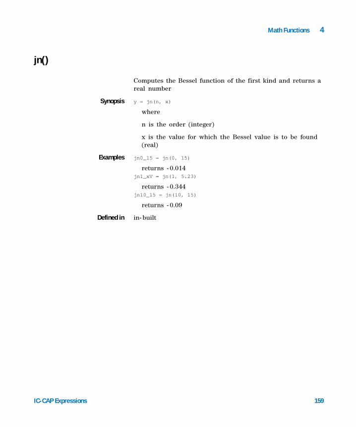
Math Functions 4
IC-CAP Expressions 159
jn()
Computes the Bessel function of the first kind and returns a real number
Synopsis y = jn(n, x)
where
n is the order (integer)
x is the value for which the Bessel value is to be found (real)
Examples jn0_15 = jn(0, 15)
returns - 0.014jn1_xV = jn(1, 5.23)
returns - 0.344jn10_15 = jn(10, 15)
returns - 0.09
Defined in in- built

160 IC-CAP Expressions
4 Math Functions
ln()
Returns the natural logarithm (ln) of an integer or real number.
Synopsis y = ln(x)
where x is the integer or real number.
Examples a = ln(e)
returns 1
Defined in Built in
See also “abs()” on page 108, “cint()” on page 119, “exp()” on page 144, “float()” on page 147, “int()” on page 154, “pow()” on page 180, “sgn()” on page 187, “sqrt()” on page 192
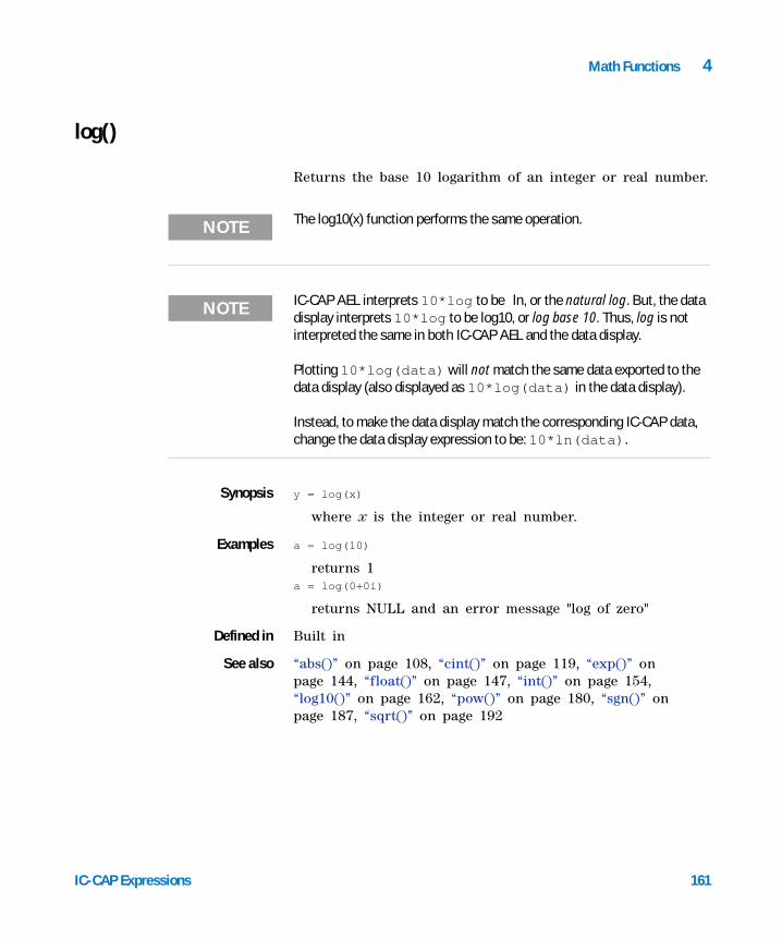
Math Functions 4
IC-CAP Expressions 161
log()
Returns the base 10 logarithm of an integer or real number.
Synopsis y = log(x)
where x is the integer or real number.
Examples a = log(10)
returns 1a = log(0+0i)
returns NULL and an error message "log of zero"
Defined in Built in
See also “abs()” on page 108, “cint()” on page 119, “exp()” on page 144, “float()” on page 147, “int()” on page 154, “log10()” on page 162, “pow()” on page 180, “sgn()” on page 187, “sqrt()” on page 192
NOTE The log10(x) function performs the same operation.
NOTE IC-CAP AEL interprets 10*log to be ln, or the natural log. But, the data display interprets 10*log to be log10, or log base 10. Thus, log is not interpreted the same in both IC-CAP AEL and the data display.
Plotting 10*log(data) will not match the same data exported to the data display (also displayed as 10*log(data) in the data display).
Instead, to make the data display match the corresponding IC-CAP data, change the data display expression to be: 10*ln(data).
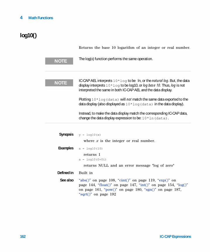
162 IC-CAP Expressions
4 Math Functions
log10()
Returns the base 10 logarithm of an integer or real number.
Synopsis y = log10(x)
where x is the integer or real number.
Examples a = log10(10)
returns 1a = log10(0+0i)
returns NULL and an error message "log of zero"
Defined in Built in
See also “abs()” on page 108, “cint()” on page 119, “exp()” on page 144, “float()” on page 147, “int()” on page 154, “log()” on page 161, “pow()” on page 180, “sgn()” on page 187, “sqrt()” on page 192
NOTE The log(x) function performs the same operation.
NOTE IC-CAP AEL interprets 10*log to be ln, or the natural log. But, the data display interprets 10*log to be log10, or log base 10. Thus, log is not interpreted the same in both IC-CAP AEL and the data display.
Plotting 10*log(data) will not match the same data exported to the data display (also displayed as 10*log(data) in the data display).
Instead, to make the data display match the corresponding IC-CAP data, change the data display expression to be: 10*ln(data).

Math Functions 4
IC-CAP Expressions 163
mag()
Returns the magnitude of a complex number.
Synopsis y = mag(x)
where x is a complex number.
Examples a = mag(3–4*j)
returns 5.000
Defined in Built in
See also “conj()” on page 122
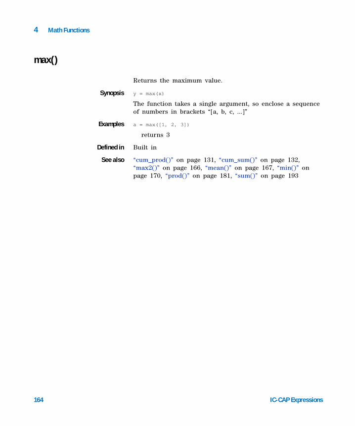
164 IC-CAP Expressions
4 Math Functions
max()
Returns the maximum value.
Synopsis y = max(x)
The function takes a single argument, so enclose a sequence of numbers in brackets “[a, b, c, ...]”
Examples a = max([1, 2, 3])
returns 3
Defined in Built in
See also “cum_prod()” on page 131, “cum_sum()” on page 132, “max2()” on page 166, “mean()” on page 167, “min()” on page 170, “prod()” on page 181, “sum()” on page 193
Math Functions 4
IC-CAP Expressions 165
max_outer()
Computes the maximum across the outer dimension of two- dimensional data.
Synopsis y = max_outer(data)
where data must be two- dimensional data.
Examples y = max_outer(data)
Defined in $ICCAP_ROOT/expressions/ael/statistcal_fun.ael
See also “fun_2d_outer()” on page 55, “mean_outer()” on page 168, “min_outer()” on page 171
Notes/Equations
The max function operates on the inner dimension of two- dimensional data. The max_outer function just calls the fun_2d_outer function, with max being the applied operation. As an example, assume that a Monte Carlo simulation of an amplifier was run, with 151 random sets of parameter values, and that for each set the S- parameters were simulated over 26 different frequency points. S21 becomes a [151 Monte Carlo iteration X 26 frequency] matrix, with the inner dimension being frequency, and the outer dimension being Monte Carlo index. Now, assume that it is desired to know the maximum value of the S- parameters at each frequency. Inserting an equation max(S21) computes the maximum value of S21 at each Monte Carlo iteration. If S21 is simulated from 1 to 26 GHz, it computes the maximum value over this frequency range, which usually is not very useful. Inserting an equation max_outer(S21) computes the maximum value of S21 at each Monte Carlo iteration.

166 IC-CAP Expressions
4 Math Functions
max2()
Returns the larger value of two numeric values, or NULL if parameters are invalid.
Synopsis z = max2(x, y)
where x is any integer or real number and y is any integer or real number.
Examples a = max2(1.5, -1.5)
returns 1.500
Defined in Built in
See also “cum_prod()” on page 131, “cum_sum()” on page 132, “max()” on page 164, “mean()” on page 167, “min()” on page 170, “prod()” on page 181, “sum()” on page 193

Math Functions 4
IC-CAP Expressions 167
mean()
Returns the mean.
Synopsis y = mean(x)
The function takes a single argument, so enclose a sequence of numbers in brackets “[a, b, c, ...]”
Examples a = mean([1, 2, 3])
returns 2
Defined in Built in
See also “cum_prod()” on page 131, “cum_sum()” on page 132, “max()” on page 164, “min()” on page 170, “prod()” on page 181, “sum()” on page 193

168 IC-CAP Expressions
4 Math Functions
mean_outer()
Computes the mean across the outer dimension of two- dimensional data.
Synopsis y = mean_outer(data)
where data must be two- dimensional data.
Examples a = mean_outer(data)
Defined in $ICCAP_ROOT/expressions/ael/statistcal_fun.ael
See also “fun_2d_outer()” on page 55, “max_outer()” on page 165, “min_outer()” on page 171
Notes/Equations
The mean function operates on the inner dimension of two- dimensional data. The mean_outer function just calls the fun_2d_outer function, with mean being the applied operation. As an example, assume that a Monte Carlo simulation of an amplifier was run, with 151 random sets of parameter values, and that for each set the S- parameters were simulated over 26 different frequency points. S21 becomes a [151 Monte Carlo iteration X 26 frequency] matrix, with the inner dimension being frequency, and the outer dimension being Monte Carlo index. Now, assume that it is desired to know the mean value of the S- parameters at each frequency. Inserting an equation mean(S21) computes the mean value of S21 at each Monte Carlo iteration. If S21 is simulated from 1 to 26 GHz, it computes the mean value over this frequency range, which usually is not very useful. Inserting an equation mean_outer(S21) computes the mean value of S21 at each Monte Carlo frequency.

Math Functions 4
IC-CAP Expressions 169
median()
Returns the median. This function can only be used by entering an equation (Eqn) in the Data Display window.
Synopsis y = median(x)
The function takes a single argument, so enclose a sequence of numbers in brackets “[a, b, c, ...]”
Examples a = median([1, 2, 3, 4])
returns 2.5
Defined in $ICCAP_ROOT/expressions/ael/statistcal_fun.ael
See also “mean()” on page 167, “sort()” on page 66
170 IC-CAP Expressions
4 Math Functions
min()
Returns the minimum value of a swept parameter.
Synopsis y = min(x)
The function takes a single argument, so enclose a sequence of numbers in brackets “[a, b, c, ...]”
Examples a = min([1, 2, 3])
returns 1
Defined in Built in
See also “cum_prod()” on page 131, “cum_sum()” on page 132, “max()” on page 164, “mean()” on page 167, “prod()” on page 181, “sum()” on page 193

Math Functions 4
IC-CAP Expressions 171
min_outer()
Computes the minimum across the outer dimension of two- dimensional data.
Synopsis y = min_outer(data)
where data must be two- dimensional data.
Examples a = min_outer(data)
Defined in $ICCAP_ROOT/expressions/ael/statistcal_fun.ael
See also “fun_2d_outer()” on page 55, “max_outer()” on page 165, “mean_outer()” on page 168
Notes/Equations
The min function operates on the inner dimension of two- dimensional data. The min_outer function just calls the fun_2d_outer function, with min being the applied operation. As an example, assume that a Monte Carlo simulation of an amplifier was run, with 151 random sets of parameter values, and that for each set the S- parameters were simulated over 26 different frequency points. S21 becomes a [151 Monte Carlo iteration X 26 frequency] matrix, with the inner dimension being frequency, and the outer dimension being Monte Carlo index. Now, assume that it is desired to know the minimum value of the S- parameters at each frequency. Inserting an equation min(S21) computes the minimum value of S21 at each Monte Carlo iteration. If S21 is simulated from 1 to 26 GHz, it computes the minimum value over this frequency range, which usually is not very useful. Inserting an equation min_outer(S21) computes the minimum value of S21 at each Monte Carlo iteration.
172 IC-CAP Expressions
4 Math Functions
min2()
Returns the lesser value of two numeric values, or NULL if parameters are invalid.
Synopsis z = min2(x, y)
where x is any integer or real number and y is any integer or real number.
Examples a = min2(1.5, -1.5)
returns - 1.500
Defined in Built in
See also “cum_prod()” on page 131, “cum_sum()” on page 132, “max()” on page 164, “max2()” on page 166, “mean()” on page 167, “min()” on page 170, “prod()” on page 181, “sum()” on page 193
Math Functions 4
IC-CAP Expressions 173
num()
Returns an integer that represents an ASCII numeric value of the first character in the specified string.
Synopsis y = num(str)
where str is a string.
Examples a = num("/users/myhome/fullpath")
returns 47
a = num("alpha")
returns 97
Defined in Built in
174 IC-CAP Expressions
4 Math Functions
ones()
Returns a matrix of ones.
Synopsis y = ones(2)
This is the ones matrix. If only one argument is supplied, then a square matrix is returned. If two are supplied, then a matrix of ones with size rows × cols is returned.
Examples a = ones(2)
returns {{1, 1}, {1, 1}}
Defined in Built in
See also “identity()” on page 151, “zeros()” on page 200
Math Functions 4
IC-CAP Expressions 175
phase()
Phase in degrees.
Synopsis y = phase(x)
Examples a = phase(1*i)
returns 90a = phase(1+1i)
returns 45
Defined in Built- in
See also “phaserad()” on page 178
176 IC-CAP Expressions
4 Math Functions
phase_comp()
Returns the phase compression (phase change).
Synopsis y = phase_comp(Sji)
where Sji is a power- dependent parameter obtained from large- signal S- parameters simulation.
Examples a = phase_comp(S21[::, 0])
Defined in $ICCAP_ROOT/expressions/ael/rf_systems_fun.ael
See also “gain_comp()” on page 212
Notes/Equations
Used in Large- signal S- parameter simulations
This measurement calculates the small- signal minus the large- signal phase, in degrees. The first power point (assumed to be small) is used to calculate the small- signal phase.

Math Functions 4
IC-CAP Expressions 177
phasedeg()
Phase in degrees.
Synopsis y = phasedeg(x)
Examples a = phasedeg(1*i)
returns 90a = phasedeg(1+1i)
returns 45
Defined in Built- in
See also “dev_lin_phase()” on page 209, “diff()” on page 139, “phase()” on page 175, “phaserad()” on page 178, “ripple()” on page 237, “unwrap()” on page 197

178 IC-CAP Expressions
4 Math Functions
phaserad()
Phase in Radians.
Synopsis y = phaserad(x)
Examples a = phaserad(1*i)
returns 1.5708a = phaserad(1+1i)
returns 0.785398
Defined in Built in
See also “dev_lin_phase()” on page 209, “diff()” on page 139, “phase()” on page 175, “phasedeg()” on page 177, “ripple()” on page 237, “unwrap()” on page 197

Math Functions 4
IC-CAP Expressions 179
polar()
Builds a complex number from magnitude and angle (in degrees).
Synopsis y = polar(mag, angle)
Examples a = polar(1, 90)
returns 0+1ia = polar(1, 45)
returns 0.707107+0.707107i
Defined in Built in
180 IC-CAP Expressions
4 Math Functions
pow()
Raises an integer or real number to a given power.
Synopsis z = pow(x, y)
where x is the integer or real number and y is the exponent of that number. x and y can be complex numbers.
Examples a = pow(4, 2)
returns 16
Defined in Built in
See also “abs()” on page 108, “cint()” on page 119, “exp()” on page 144, “float()” on page 147, “int()” on page 154, “log10()” on page 162, “sgn()” on page 187, “sqrt()” on page 192

Math Functions 4
IC-CAP Expressions 181
prod()
Returns the product.
Synopsis y = prod(x)
where x can be an integer, real, or complex number.
Examples a = prod([1, 2, 3]
returns 6a = prod([4, 4, 4])
returns 64
Defined in Built- in
See also “sum()” on page 193
182 IC-CAP Expressions
4 Math Functions
rad()
Degrees to radians.
Synopsis y = rad(x)
Examples a = rad(90)
returns 1.5708a = rad(45)
returns 0.785398
Defined in Built in
See also “deg()” on page 137
Math Functions 4
IC-CAP Expressions 183
re()
Returns a real number, the real part of a complex value.
Synopsis y = re(x)
where x is a complex number.
Examples a = re(1–1*j)
returns 1.000
Defined in Built in
See also “cmplx()” on page 120, “imag()” on page 153, “real()” on page 184
NOTE The real() function performs the same operation.
184 IC-CAP Expressions
4 Math Functions
real()
Returns the real part of a complex number.
Synopsis y = real(x)
where x is a complex number.
Examples a = real(1–1*j)
returns 1.000
Defined in Built in
See also “cmplx()” on page 120, “imag()” on page 153, “re()” on page 183
NOTE The re() function performs the same operation.
Math Functions 4
IC-CAP Expressions 185
rms()
Returns the root mean square value.
Synopsis y = rms(val)
where val is an integer, real, or complex number.
Examples rmsR = rms(2)
returns 1.414rmsR = rms(complex(3, 10))
returns 7.382/73.301rmsR = rms( [1, 2, 3, 4, 5,] )
returns [0.707, 1.414, 2.121, 2.828, 3.536]
Defined in $HPEESOF_DIR/expressions/ael/elementary_fun.ael
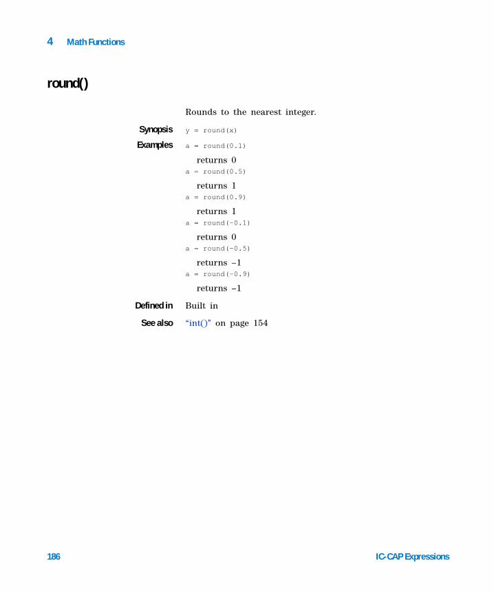
186 IC-CAP Expressions
4 Math Functions
round()
Rounds to the nearest integer.
Synopsis y = round(x)
Examples a = round(0.1)
returns 0a = round(0.5)
returns 1a = round(0.9)
returns 1a = round(–0.1)
returns 0a = round(–0.5)
returns –1a = round(–0.9)
returns –1
Defined in Built in
See also “int()” on page 154
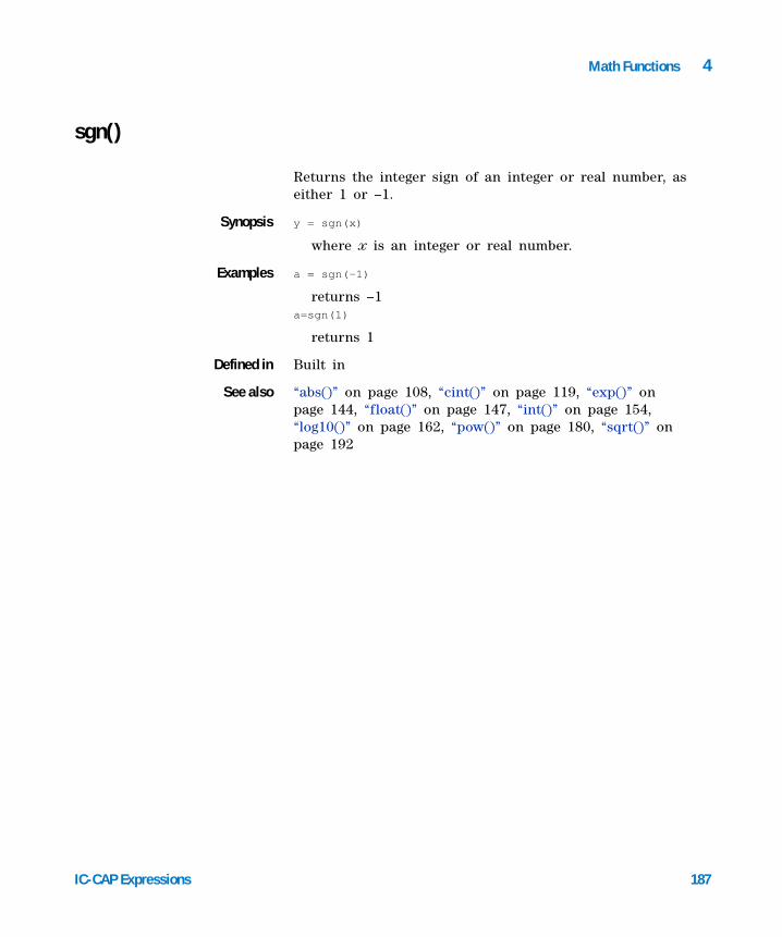
Math Functions 4
IC-CAP Expressions 187
sgn()
Returns the integer sign of an integer or real number, as either 1 or –1.
Synopsis y = sgn(x)
where x is an integer or real number.
Examples a = sgn(–1)
returns –1a=sgn(1)
returns 1
Defined in Built in
See also “abs()” on page 108, “cint()” on page 119, “exp()” on page 144, “float()” on page 147, “int()” on page 154, “log10()” on page 162, “pow()” on page 180, “sqrt()” on page 192

188 IC-CAP Expressions
4 Math Functions
sin()
Returns the sine of an integer or real number.
Synopsis y = sin(x)
where x is an integer or real number, in radians.
Examples a = sin(pi/2)
returns 1
Defined in Built in
See also “cos()” on page 127, “tan()” on page 194
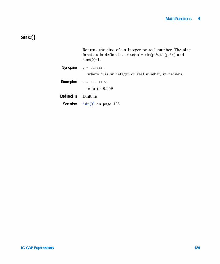
Math Functions 4
IC-CAP Expressions 189
sinc()
Returns the sinc of an integer or real number. The sinc function is defined as sinc(x) = sin(pi*x)/ (pi*x) and sinc(0)=1.
Synopsis y = sinc(x)
where x is an integer or real number, in radians.
Examples a = sinc(0.5)
returns 0.959
Defined in Built in
See also “sin()” on page 188

190 IC-CAP Expressions
4 Math Functions
sinh()
Returns the hyperbolic sin of an integer or real number.
Synopsis y = sinh(x)
where x is an integer or real number, in radians.
Examples a = sinh(0)
returns 0a = sinh(1)
returns 1.1752
Defined in Built in
See also “cosh()” on page 128, “tanh()” on page 195

Math Functions 4
IC-CAP Expressions 191
sqr()
Returns the square of a number.
Synopsis y=sqr(x)
where x is the number to square. Any integer, real, or complex value for x is allowed.
Examples y = sqr(2)
returns 4
Defined In $HPEESOF_DIR/expressions/ael/elementary_fun.ael

192 IC-CAP Expressions
4 Math Functions
sqrt()
Returns the square root of a positive integer or real number.
Synopsis y = sqrt(x)
where x is a positive integer or real number.
Examples a = sqrt(4)
returns 2
Defined in Built in
See also “abs()” on page 108, “cint()” on page 119, “exp()” on page 144, “float()” on page 147, “int()” on page 154, “log10()” on page 162, “pow()” on page 180, “sgn()” on page 187

Math Functions 4
IC-CAP Expressions 193
sum()
Returns the sum.
Synopsis y = sum(x)
The function takes a single argument, so enclose a sequence of numbers in brackets “[a, b, c, ...]”
Examples a = sum([1, 2, 3])
returns 6
Defined in Built in
See also “max()” on page 164, “mean()” on page 167, “min()” on page 170
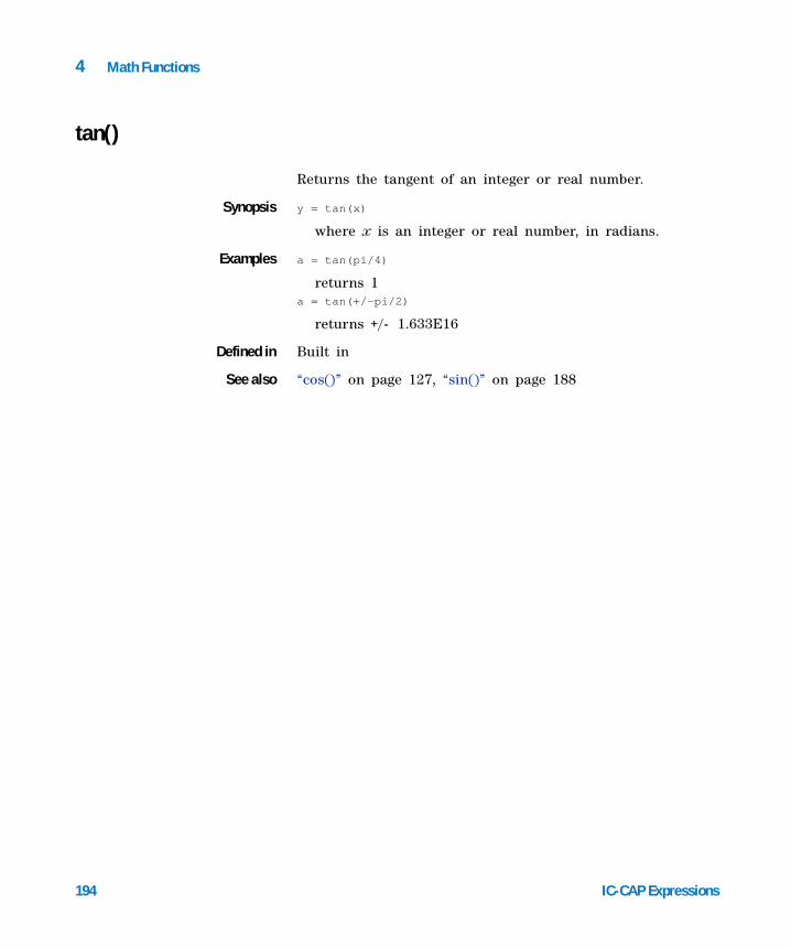
194 IC-CAP Expressions
4 Math Functions
tan()
Returns the tangent of an integer or real number.
Synopsis y = tan(x)
where x is an integer or real number, in radians.
Examples a = tan(pi/4)
returns 1a = tan(+/-pi/2)
returns +/- 1.633E16
Defined in Built in
See also “cos()” on page 127, “sin()” on page 188

Math Functions 4
IC-CAP Expressions 195
tanh()
Returns the hyperbolic tangent of an integer or real number.
Synopsis y = tanh(x)
where x is an integer or real number, in radians.
Examples a = tanh(0)
returns 0a = tanh(1)
returns 0.761594a = tanh(–1)
returns –0.761594
Defined in Built in
See also “cosh()” on page 128, “sinh()” on page 190

196 IC-CAP Expressions
4 Math Functions
transpose()
Transposes a matrix.
Synopsis Y = transpose(y)
This function transposes a matrix, but does not perform a conjugate transpose for complex matrices.
Examples a={{1, 2}, {3, 4}}b=transpose(a)
returns {{1, 3}, {2, 4}}
Defined in Built in
Math Functions 4
IC-CAP Expressions 197
unwrap()
This measurement unwraps a phase by changing an absolute jump greater than jump to its 2*jump complement.
Synopsis y = unwrap(phase{, jump})
where
phase is a swept real variable.
jump is the absolute jump. By default, jump is set to 180.
Examples a = unwrap(phase(S21))a = unwrap(phaserad(S21), pi)
Defined in Built- in
See also “dev_lin_phase()” on page 209, “diff()” on page 139, “phase()” on page 175, “phasedeg()” on page 177, “phaserad()” on page 178, “ripple()” on page 237
NOTE The unit used is in degrees.

198 IC-CAP Expressions
4 Math Functions
wtodbm()
Converts Watts to dBm and returns a real or complex number.
Synopsis dbmVal = wtodbm(Value)
where
Value is an integer, real or complex number.
Examples wtodbm01_M=wtodbm(0.01)
returns 10wtodbm1_M=wtodbm(1)
returns 30wtodbmC_M=wtodbm(complex(10,2))
returns 40.094/1.225
Defined in $HPEESOF_DIR/expressions/ael/elementary_fun.ael
See also “dbmtow()” on page 136

Math Functions 4
IC-CAP Expressions 199
xor()
Returns an integer that represents the exclusive OR between arguments.
Synopsis z = xor(x, y)
where x is any integer and y is any integer.
Examples a = xor(16, 32)
returns 48
Defined in Built in

200 IC-CAP Expressions
4 Math Functions
zeros()
Returns a matrix of zeros.
Synopsis Y = zeros(2)Y = zeros(2, 3)
This is the zeros matrix. If only one argument is supplied, then a square matrix is returned. If two are supplied, then a matrix of zeros with size rows x cols is returned.
Examples a=zeros(2)
returns {{0, 0}, {0, 0}}b=(2, 3)
returns {{0, 0, 0}, {0, 0, 0}}
Defined in Built in
See also “identity()” on page 151, “ones()” on page 174
201
Agilent 85190A IC-CAP 2006Expressions
Agilent Technologies
5S-parameter Analysis Functions
A, B, C, D, Gabcdtoh() 203
abcdtos() 204
abcdtoy() 205
abcdtoz() 206
bandwidth_func() 207
center_freq() 208
dev_lin_phase() 209
ga_circle() 210
gain_comp() 212
gl_circle() 213
gp_circle() 215
gs_circle() 217
H, I, L, Mhtoabcd() 219
htos() 220
htoy() 221
htoz() 222ispec() 223
l_stab_circle() 224
l_stab_circle_center_radius() 225
l_stab_region() 226
map1_circle() 227
map2_circle() 228
max_gain() 229
mu() 230
mu_prime() 231
N, P, Rns_circle() 232
ns_pwr_int() 234
ns_pwr_ref_bw() 235
pwr_gain() 236
ripple() 237
202 IC-CAP Expressions
5 S-parameter Analysis Functions
This chapter describes the S- parameter analysis functions in detail. The functions are listed in alphabetical order.
Ss_stab_circle() 238
s_stab_circle_center_radius() 239
s_stab_region() 240
sm_gamma1() 241
sm_gamma2() 242
sm_y1() 243
sm_y2() 244
sm_z1() 245
sm_z2() 246
stab_fact() 247
stab_meas() 248
stoabcd() 249
stoh() 250
stos() 251
stot() 252
stoy() 253
stoz() 254
T,U,V,W,Ytdr_sp_gamma() 255
tdr_sp_imped() 256
tdr_step_imped() 257
ttos() 258
unilateral_figure() 259
volt_gain() 261
volt_gain_max() 263
vswr() 264
write_snp() 265
yin() 267
yopt() 268
ytoabcd() 269
ytoh() 270
ytos() 271
ytoz() 272
Zzin() 273
zopt() 274
ztoabcd() 275
ztoh() 276
ztos() 277
ztoy() 278

S-parameter Analysis Functions 5
IC-CAP Expressions 203
abcdtoh()
This measurement transforms the chain (ABCD) matrix of a 2- port network to a hybrid matrix.
Synopsis y = abcdtoh(A)
where A is the chain (ABCD) matrix of a 2- port network.
Examples h=abcdtoh(a)
Defined in $ICCAP_ROOT/expressions/ael/network_fun.ael
See also “abcdtos()” on page 204, “abcdtoy()” on page 205, “abcdtoz()” on page 206, “htoabcd()” on page 219, “stoabcd()” on page 249, “ytoabcd()” on page 269, “ztoabcd()” on page 275

204 IC-CAP Expressions
5 S-parameter Analysis Functions
abcdtos()
This measurement transforms the chain (ABCD) matrix of a 2- port network to a scattering matrix.
Synopsis y = abcdtos(A, zRef)
where A is the chain (ABCD) matrix of a 2- port network and zRef is a reference impedance.
Examples s = abcdtos(a, 50)
Defined in $ICCAP_ROOT/expressions/ael/network_fun.ael
See also “abcdtoh()” on page 203, “abcdtoy()” on page 205, “abcdtoz()” on page 206, “htoabcd()” on page 219, “stoabcd()” on page 249, “ytoabcd()” on page 269, “ztoabcd()” on page 275
S-parameter Analysis Functions 5
IC-CAP Expressions 205
abcdtoy()
This measurement transforms the chain (ABCD) matrix of a 2- port network to an admittance matrix.
Synopsis y = abcdtoy(A)
where A is the chain (ABCD) matrix of a 2- port network.
Examples y = abcdtoy(a)
Defined in $ICCAP_ROOT/expressions/ael/network_fun.ael
See also “abcdtoh()” on page 203, “abcdtos()” on page 204, “abcdtoz()” on page 206, “htoabcd()” on page 219, “stoabcd()” on page 249, “ytoabcd()” on page 269, “ztoabcd()” on page 275

206 IC-CAP Expressions
5 S-parameter Analysis Functions
abcdtoz()
This measurement transforms the chain (ABCD) matrix of a 2- port network to impedance matrix.
Synopsis y = abcdtoz(A)
where A is the chain (ABCD) matrix of a 2- port network.
Examples z = abcdtoz(a)
Defined in $ICCAP_ROOT/expressions/ael/network_fun.ael
See also “abcdtoh()” on page 203, “abcdtos()” on page 204, “abcdtoy()” on page 205, “htoabcd()” on page 219, “stoabcd()” on page 249, “ytoabcd()” on page 269, “ztoabcd()” on page 275

S-parameter Analysis Functions 5
IC-CAP Expressions 207
bandwidth_func()
Returns the bandwidth at the specified level as a real number. Typically used in filter application to calculate the 1, 3 dB, etc. bandwidth.
Synopsis bw = bandwidth(Data, DesiredValue {, Bandstop})
where
Data is (usually gain) to find the bandwidth.
DesiredValue is a single value representing the desired bandwidth level.
Bandstop is an optional argument set to 1 to calculate the bandstop response rather than the bandpass.
Examples This example assumes that an S- parameter analysis has been performed.bw3dB = bandwidth_func(db(S21), 3)
returns the 3dB bandwidth
Defined in $HPEESOF_DIR/expressions/ael/rf_system_fun.ael
See also “center_freq()” on page 208
Notes/Equations
This function returns the bandwidth of a filter response. Linear interpolation is done between data points. Uses an iterative process to find the bandwidth on non- ideal responses. The data can be from 1 to 4 dimensions.
208 IC-CAP Expressions
5 S-parameter Analysis Functions
center_freq()
Returns the center frequency at the specified level as a real number. Typically used in filter application to calculate the center frequency at 1, 3 dB, etc. bandwidth.
Synopsis fc = center_freq(Data, DesiredBW)
where
Data is (usually gain) to find the center frequency.
DesiredBW is a single value representing the reference bandwidth.
Examples This example assumes that an S- parameter analysis has been performed.fc3 = center_freq(db(S21), 3)
returns the center frequency using the 3dB point as reference.
Defined in $HPEESOF_DIR/expressions/ael/rf_system_fun.ael
See also “bandwidth_func()” on page 207
Notes/Equations
This function returns the center frequency of a filter response. Linear interpolation is done between data points. Uses an iterative process to find the bandwidth on non- ideal responses. The data can be from 1 to 4 dimensions.
S-parameter Analysis Functions 5
IC-CAP Expressions 209
dev_lin_phase()
Given a variable sweep over a frequency range, a linear least- squares fit is performed on the phase of the variable, and the deviation from this linear fit is calculated at each frequency point.
Synopsis y = dev_lin_phase(voltGain)
where voltGain is a function of frequency.
Examples a = dev_lin_phase(S21)
Defined in $ICCAP_ROOT/expressions/ael/rf_system_fun.ael
See also “diff()” on page 139, “phasedeg()” on page 177, “phaserad()” on page 178, “pwr_gain()” on page 236, “ripple()” on page 237, “unwrap()” on page 197, “volt_gain()” on page 261

210 IC-CAP Expressions
5 S-parameter Analysis Functions
ga_circle()
Generates an available- gain circle.
Synopsis y = ga_circle(S{, gain, numOfPts, numCircles, gainStep})
where
S is the scattering matrix of a 2- port network.
gain is the specified gain in dB. The default value for gain is min(max_gain(S)) - {0, 1, 2, 3}.
numOfPts is the desired number of points per circle. The default value for numOfPts is 51.
numCircles is the number of desired circles. This is used if gain is not specified.
gainStep is the gain step size. This is used if gain is not specified. Default = 1.0.
Examples circleData = ga_circle(S, 2, 51)circleData = ga_circle(S, {2, 3, 4}, 51)
returns the points on the circle(s).circleData = ga_circle(S, , 51, 5, 0.5)
returns the points on the circle(s) for 5 circles at maxGain - {0,0.5,1.0,1.5,2.0}
circleData = ga_circle(S, , , 2, 1.0)
returns the points on the circle(s) for 2 circles at maxGain - {0,1.0}
Used in Small- signal S- parameter simulations
Available asmeasurement
component?
GaCircle
Defined in $ICCAP_ROOT/expressions/ael/circle_fun.ael
See also “gl_circle()” on page 213, “gp_circle()” on page 215, “gs_circle()” on page 217
S-parameter Analysis Functions 5
IC-CAP Expressions 211
Description This function generates the constant available- gain circle resulting from a source mismatch. The circle is defined by the loci of the source- reflection coefficients resulting in the specified gain.
A gain circle is created for each value of the swept variable(s). Multiple gain values can be specified for a scattering parameter that has dimension less than four. This measurement is supported for 2- port networks only.
If gain is not specified, and if numCircles is not specified as well gain circles are drawn at min(max_gain(S)) - {0,1,2,3}. That is gain is calculated at a loss of 0,1,2,3 dB from maxGain. If gain is not specified, and if numCircles is given then numCircles gain circles are drawn at gainStep below max_gain(). Gain is also limited by max_gain(S) (i.e., is gain > max_gain(S), then the circle is generated at max_gain(S)).

212 IC-CAP Expressions
5 S-parameter Analysis Functions
gain_comp()
Returns gain compression.
Synopsis y = gain_comp(Sji)
where Sji is a power- dependent complex transmission coefficient obtained from large- signal S- parameter simulation.
Examples gc = gain_comp(S21[::, 0])
Defined in $ICCAP_ROOT/expressions/ael/rf_system_fun.ael
See also “phase_comp()” on page 176
Notes/Equations
Used in Large- signal S- parameter simulations
This measurement calculates the small- signal minus the large- signal power gain, in dB. The first power point (assumed to be small) is used to calculate the small- signal power gain.
S-parameter Analysis Functions 5
IC-CAP Expressions 213
gl_circle()
Generates a load- mismatch gain circle.
Synopsis y =gl_circle(S{, gain, numOfPts, numCircles, gainStep})
where
S is the scattering matrix of a 2- port network
gain is the specified gain in dB. The default value for gain is maxGain – {0, 1, 2, 3}.
Where maxGain = 10*log(1 / (1 - mag(S22)**2))
numOfPts is the desired number of points per circle. The default value for numOfPts is 51.
numCircles is the number of desired circles. This is used if gain is not specified.
gainStep is the gain step size. This is used if gain is not specified. Default = 1.0.
Examples circleData = gl_circle(S, 2, 51)circleData = gl_circle(S, {2, 3, 4}, 51)
returns the points on the circle(s).circleData = gl_circle(S, , 51, 5, 0.5)
returns the points on the circle(s) for 5 circles at maxGain - {0,0.5,1.0,1.5,2.0}
circleData = gl_circle(S, , , 2, 1.0)
returns the points on the circle(s) for 2 circles at maxGain - {0,1.0}
Used in Small- signal S- parameter simulations
Defined in $ICCAP_ROOT/expressions/ael/circle_fun.ael
See also “ga_circle()” on page 210, “gp_circle()” on page 215, “gs_circle()” on page 217
Description This expression generates the unilateral gain circle resulting from a load mismatch. The circle is defined by the loci of the load- reflection coefficients that result in the specified gain.

214 IC-CAP Expressions
5 S-parameter Analysis Functions
A gain circle is created for each value of the swept variable(s). Multiple gain values can be specified for a scattering parameter that has dimension less than four. This measurement is supported for 2- port networks only.
If gain is not specified, and if numCircles is not specified as well gain circles are drawn at maxGain – {0,1,2,3}. That is gain is calculated at a loss of 0,1,2,3 dB from the maximum gain. If gain is not specified, and if numCircles is given then numCircles gain circles are drawn at gainStep below maxGain. Gain is also limited by maxGain (i.e., if gain > maxGain, then the circle is generated at maxGain).

S-parameter Analysis Functions 5
IC-CAP Expressions 215
gp_circle()
Generates a power gain circle.
Synopsis y = gp_circle(S{, gain, numOfPts, numCircles, gainStep})
where
S is the scattering matrix of a 2- port network.
gain is the specified gain in dB. The default value for gain is min(max_gain(S)) − {1, 2, 3}.
numOfPts is the desired number of points per circle. The default value for numOfPts is 51.
numCircles is the number of desired circles. This is used if gain is not specified.
gainStep is the gain step size. This is used if gain is not specified. Default = 1.0.
Examples circleData = gp_circle(S, 2, 51)circleData = gp_circle(S, {2, 3, 4}, 51)
returns the points on the circle(s).circleData = gp_circle(S, , 51, 5, 0.5)
returns the points on the circle(s) for 5 circles at maxGain – {0,0.5,1.0,1.5,2.0}
circleData = gp_circle(S, , , 2, 1.0)
returns the points on the circle(s) for 2 circles at maxGain – {0,1.0}
Used in Small- signal S- parameter simulations
Defined in $ICCAP_ROOT/expressions/ael/circle_fun.ael
See also “ga_circle()” on page 210, “gl_circle()” on page 213, “gs_circle()” on page 217
Description This expression generates a constant- power- gain circle resulting from a load mismatch. The circle is defined by the loci of the output- reflection coefficients that result in the specified gain.

216 IC-CAP Expressions
5 S-parameter Analysis Functions
A gain circle is created for each value of the swept variable(s). Multiple gain values can be specified for a scattering parameter that has dimension less than four. This measurement is supported for 2- port networks only.
If gain is not specified, and if numCircles is not specified as well gain circles are drawn at min(max_gain(S)) – {0,1,2,3}. That is gains are calculated at a loss of 0,1,2,3 dB from the maximum gain. If gain is not specified, and if numCircles is given then numCircles gain circles are drawn at gainStep below max_gain(). Gain is also limited by max_gain(S) (i.e., if gain > max_gain(S), then the circle is generated at max_gain(S)).

S-parameter Analysis Functions 5
IC-CAP Expressions 217
gs_circle()
Returns a source- mismatch gain circle.
Synopsis y = gs_circle(S{, gain, numOfPts, numCircles, gainStep})
where
S is the scattering matrix of a 2- port network.
gain is the specified gain in dB. The default value for gain is maxGain – {0, 1, 2, 3}.
Where maxGain = 10*log(1 / (1 - mag(S11)**2))
numOfPts is the desired number of points per circle. The default value for numOfPts is 51.
numCircles is the number of desired circles. This is used if gain is not specified.
gainStep is the gain step size. This is used if gain is not specified. Default = 1.0.
Examples circleData = gs_circle(S, 2, 51)circleData = gs_circle(S, {2, 3, 4}, 51)
returns the points on the circle(s).circleData = gs_circle(S, , 51, 5, 0.5)
returns the points on the circle(s) for 5 circles at maxGain - {0,0.5,1.0,1.5,2.0}
circleData = gs_circle(S, , , 2, 1.0)
returns the points on the circle(s) for 2 circles at maxGain - {0,1.0}
Used in Small- signal S- parameter simulations
Defined in $ICCAP_ROOT/expressions/ael/circle_fun.ael
See also “ga_circle()” on page 210, “gl_circle()” on page 213, “gp_circle()” on page 215
Description This expression generates the unilateral gain circle resulting from a source mismatch. The circle is defined by the loci of the source- reflection coefficients that result in the specified gain.

218 IC-CAP Expressions
5 S-parameter Analysis Functions
A gain circle is created for each value of the swept variable(s). Multiple gain values can be specified for a scattering parameter that has dimension less than four. This measurement is supported for 2- port networks only.
If gain is not specified, and if numCircles is not specified as well gain circles are drawn at maxGain – {0,1,2,3}. That is gain values are calculated at a loss of 0,1,2,3 dB from the maximum gain. If gain is not specified, and if numCircles is given then numCircles gain circles are drawn at gainStep below maxGain. Gain is also limited by maxGain (i.e., if gain > maxGain, then the circle is generated at maxGain).

S-parameter Analysis Functions 5
IC-CAP Expressions 219
htoabcd()
This measurement transforms the hybrid matrix of a 2- port network to a chain (ABCD) matrix.
Synopsis y = htoabcd(H)
where H is the hybrid matrix of a 2- port network.
Examples a = htoabcd(h)
Defined in $ICCAP_ROOT/expressions/ael/network_fun.ael
See also “abcdtoh()” on page 203, “htoz()” on page 222, “ytoh()” on page 270
220 IC-CAP Expressions
5 S-parameter Analysis Functions
htos()
This measurement transforms the hybrid matrix of a 2- port network to a scattering matrix.
Synopsis y = htos(H, Z)
where
H is the hybrid matrix of a 2- port network.
Z is the reference impedance.
Examples s = htos(h, 50)
Defined in $ICCAP_ROOT/expressions/ael/network_fun.ael
See also “htoy()” on page 221, “htoz()” on page 222, “stoh()” on page 250

S-parameter Analysis Functions 5
IC-CAP Expressions 221
htoy()
This measurement transforms the hybrid matrix of a 2- port network to an admittance matrix.
Synopsis y = htoy(H)
where H is the hybrid matrix of a 2- port network.
Examples y = htoy(H)
Defined in $ICCAP_ROOT/expressions/ael/network_fun.ael
See also “htos()” on page 220, “htoz()” on page 222, “ytoh()” on page 270

222 IC-CAP Expressions
5 S-parameter Analysis Functions
htoz()
This measurement transforms the hybrid matrix of a 2- port network to an impedance matrix.
Synopsis y = htoz(H)
where H is the hybrid matrix of a 2- port network.
Examples z = htoz(h)
Defined in $ICCAP_ROOT/expressions/ael/network_fun.ael
See also “htos()” on page 220, “htoy()” on page 221, “ytoh()” on page 270

S-parameter Analysis Functions 5
IC-CAP Expressions 223
ispec()
Returns the current frequency spectrum.
Synopsis y=ispec(current)
where current is the current for which a frequency spectrum is returned. The allowed types are real or complex. All values are allowed.
Examples a = ispec(i1)
Defined In $HPEESOF_DIR/expressions/ael/circuit_fun.ael
Notes/Equations
This measurement gives a current frequency spectrum. The measurement gives a set of RMS currents at each frequency.

224 IC-CAP Expressions
5 S-parameter Analysis Functions
l_stab_circle()
Returns a load (output) stability circle.
Synopsis y = l_stab_circle(S{, numOfPts})
where
S is the scattering matrix of a 2- port network.
numOfPts is the desired number of points per circle and is set to 51 by default.
Examples circleData = l_stab_circle(S, 51)
returns the points on the circle(s).
Used in Small- signal S- parameter simulations
Defined in $ICCAP_ROOT/expressions/ael/circle_fun.ael
See also “l_stab_region()” on page 226, “s_stab_circle()” on page 238, “s_stab_region()” on page 240
Notes/Equations
The expression generates a load stability circle. The circle is defined by the loci of load- reflection coefficients where the magnitude of the source- reflection coefficient is 1.
A circle is created for each value of the swept variable(s). This measurement is supported for 2- port networks only.

S-parameter Analysis Functions 5
IC-CAP Expressions 225
l_stab_circle_center_radius()
Returns the center and radius of the load (output) stability circle.
Synopsis y = l_stab_circle_center_radius(S, {Type})
where
S is the scattering matrix of a 2- port network.
Type is the type of parameter to return – “center”, “radius”. Default “both”.
Examples l_cr=l_stab_circle_center_radius(S)
returns a 1X2 matrix containing center and radius.lCirc=expand(circle(l_cr(1), real(l_cr(2)), 51))
returns data for the load stability circle.l_radius=l_stab_circle_center_radius(S, “radius”)
returns the radius.
Used in Small- signal S- parameter simulations
Available asmeasurement
component?
Not available
Defined in $ICCAP_ROOT/expressions/ael/circle_fun.ael
See also “l_stab_circle()” on page 224, “s_stab_circle()” on page 238, “s_stab_circle_center_radius()” on page 239
Description If the argument Type is not specified, the function returns complex data. Although radius is of type real, the values are returned as complex. Therefore, when using the returned radius, use the real part. To obtain the radius as a real number, set “Type” to radius.
226 IC-CAP Expressions
5 S-parameter Analysis Functions
l_stab_region()
This expression returns a string identifying the region of stability of the corresponding load stability circle.
Synopsis y = l_stab_region(S)
where S is the scattering matrix of a 2- port network.
Examples region = l_stab_region(S)
returns “Outside” or “Inside”.
Defined in $ICCAP_ROOT/expressions/ael/circle_fun.ael
See also “l_stab_circle()” on page 224, “s_stab_circle()” on page 238, “s_stab_region()” on page 240
Notes/Equations
Used in Small- signal S- parameter simulations
S-parameter Analysis Functions 5
IC-CAP Expressions 227
map1_circle()
Returns source- mapping circles from port 1 to port 2.
Synopsis circleData=map1_circle(S{, numOfPts})
where
S is the scattering matrix of a 2- port network.
numOfPts is the desired number of points per circle and is set to 51 by default.
Examples circleData=map1_circle(S, 51)
returns the points on the circle(s).
Defined in $ICCAP_ROOT/expressions/ael/circles_fun.ael
See also “map2_circle()” on page 228
Notes/Equations
Used in Small- signal S- parameter simulations
The expression maps the set of terminations with unity magnitude at port 1 to port 2. The circles are defined by the loci of terminations on one port as seen at the other port.
A source- mapping circle is created for each value of the swept variable(s). This measurement is supported for 2- port networks only.

228 IC-CAP Expressions
5 S-parameter Analysis Functions
map2_circle()
Returns source- mapping circles, from port 2 to port 1
Synopsis circleData=map2_circle(S{, numOfPts})
where
S is the scattering matrix of a 2- port network.
numOfPts is the desired number of points per circle and is set to 51 by default.
Examples circleData=map2_circle(S, 51)
returns the points on the circle(s).
Defined in $ICCAP_ROOT/expressions/ael/circle_fun.ael
See also “map1_circle()” on page 227
Notes/Equations
Used in Small- signal S- parameter simulations
The expression maps the set of terminations with unity magnitude at port 2 to port 1. The circles are defined by the loci of terminations on one port as seen at the other port.
A source- mapping circle is created for each value of the swept variable(s). This measurement is supported for 2- port networks only.
S-parameter Analysis Functions 5
IC-CAP Expressions 229
max_gain()
Given a 2 x 2 scattering matrix, this measurement returns the maximum available and stable gain (in dB) between the input and the measurement ports.
Synopsis y = max_gain(S)
where S is a scattering matrix of 2- port network.
Examples y = max_gain(S)
Defined in $ICCAP_ROOT/expressions/ael/rf_system_fun.ael
See also “sm_gamma1()” on page 241, “sm_gamma2()” on page 242, “stab_fact()” on page 247, “stab_meas()” on page 248

230 IC-CAP Expressions
5 S-parameter Analysis Functions
mu()
Returns the geometrically derived stability factor for the load.
Synopsis y = mu(S)
where S is a scattering matrix of a 2- port network.
Examples x=mu(S)
Defined in $ICCAP_ROOT/expressions/ael/circuit_fun.ael
See also “mu_prime()” on page 231
Notes/Equations
This measurement gives the distance from the center of the Smith chart to the nearest output (load) stability circle.
This stability factor is given by
mu = {1- |S11|**2} / {|S22 - conj(S11)*Delta | + |S12*S21| }
where Delta is the determinant of the S- parameter matrix. Having mu > 1 is the single necessary and sufficient condition for unconditional stability of the 2- port network.
Reference 1 M. L. Edwards and J. H. Sinsky, “A new criterion for linear 2- port stability using geometrically derived parameters", IEEE Transactions on Microwave Theory and Techniques, Vol. 40, No. 12, pp. 2303- 2311, Dec. 1992.
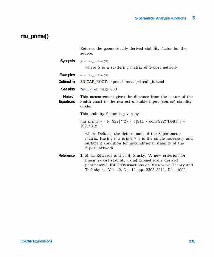
S-parameter Analysis Functions 5
IC-CAP Expressions 231
mu_prime()
Returns the geometrically derived stability factor for the source.
Synopsis y = mu_prime(S)
where S is a scattering matrix of 2- port network.
Examples a = mu_prime(S)
Defined in $ICCAP_ROOT/expressions/ael/circuit_fun.ael
See also “mu()” on page 230
Notes/Equations
This measurement gives the distance from the center of the Smith chart to the nearest unstable- input (source) stability circle.
This stability factor is given by
mu_prime = {1- |S22|**2} / {|S11 - conj(S22)*Delta | + |S21*S12| }
where Delta is the determinant of the S- parameter matrix. Having mu_prime > 1 is the single necessary and sufficient condition for unconditional stability of the 2- port network.
Reference 1 M. L. Edwards and J. H. Sinsky, “A new criterion for linear 2- port stability using geometrically derived parameters”, IEEE Transactions on Microwave Theory and Techniques, Vol. 40, No. 12, pp. 2303- 2311, Dec. 1992.

232 IC-CAP Expressions
5 S-parameter Analysis Functions
ns_circle()
Returns noise- figure circles.
Synopsis y = ns_circle(nf, NFmin, Sopt, rn{, numOfPts, numCircles, NFStep})
where
nf is the specified noise figure and is set by default to max(NFmin) + {0, 1, 2, 3}.
NFmin is the minimum noise figure.
Sopt is the optimum mismatch.
rn is the equivalent normalized noise resistance of a 2- port network (rn = Rn/zRef where Rn is the equivalent noise resistance and zRef is the reference impedance).
numOfPts is the desired number of points per circle and is set to 51 by default.
numCircles is the number of desired circles. This is used if nf is not specified.
NFStep is the nf step size. This is used if nf is not specified. Default = 1.0.
Examples circleData = ns_circle(0+NFmin, NFmin, Sopt, Rn/50, 51). circleData = ns_circle({0, 1}+NFmin, NFmin, Sopt, Rn/50, 51)
returns the points on the circle(s). circleData = ns_circle(, NFmin, Sopt, Rn/50, 51, 3, 0.5)
returns the points on the circle(s) for 3 circles at max(NFmin) + {0, 0.5, 1.0}.
circleData = ns_circle(, NFmin, Sopt, Rn/50, , 3)
returns the points on the circle(s) for 3 circles at max(NFmin) + {0, 1, 2.0}.
Used in Small- signal S- parameter simulations
Available asmeasurement
component?
NsCircle
Defined in $ICCAP_ROOT/expressions/ael/circle_fun.ael

S-parameter Analysis Functions 5
IC-CAP Expressions 233
Description The expression generates constant noise- figure circles. The circles are defined by the loci of the source- reflection coefficients that result in the specified noise figure. NFmin, Sopt, and Rn are generated from noise analysis.
A circle is created for each value of the swept variable(s).
If nf is not specified, and if numCircles is not specified as well nf circles are drawn at max(NFmin) + {0,1,2,3}. If nf is not specified, and if numCircles is given then numCircles nf circles are drawn at NFStep above max(NFmin).

234 IC-CAP Expressions
5 S-parameter Analysis Functions
ns_pwr_int()
Returns the integrated noise power.
Synopsis y = ns_pwr_int(Sji, nf, resBW)
where
Sji is the complex transmission coefficient.
nf is noise figure at the output port (in dB).
resBW is the user- defined resolution bandwidth.
Examples Y = ns_pwr_int(S21, nf2, 1MHz)
Defined in $ICCAP_ROOT/expressions/ael/rf_system_fun.ael
See also “ns_pwr_ref_bw()” on page 235, “snr()” on page 94
Notes/Equations
Used in Small- signal S- parameter simulation
This is the integrated noise power (in dBm) calculated by integrating the noise power over the entire frequency sweep. The noise power at each frequency point is calculated by multiplying the noise spectral density by a user- defined resolution bandwidth.

S-parameter Analysis Functions 5
IC-CAP Expressions 235
ns_pwr_ref_bw()
Returns noise power in a reference bandwidth.
Synopsis y = ns_pwr_ref_bw(Sji, nf, resBW)
where
Sji is the complex transmission coefficient.
nf is noise figure at the output port (in dB).
resBW is the user- defined resolution bandwidth.
Examples Y = ns_pwr_ref_bw(S21, nf2, 1MHz)
returns the noise power with respect to the reference bandwidth.
Defined in $ICCAP_ROOT/expressions/ael/rf_system_fun.ael
See also “ns_pwr_int()” on page 234, “snr()” on page 94
Notes/Equations
Used in Small- signal S- parameter simulation
This is the noise power calculated by multiplying the noise spectral density at a frequency point by a user- defined resolution bandwidth. Unlike NsPwrInt, this gives the noise power (in dB) at each frequency sweep.
236 IC-CAP Expressions
5 S-parameter Analysis Functions
pwr_gain()
This measurement is used to determine the transducer power gain (in dB) and is defined as the ratio of the power delivered to the load, to the power available from the source. (where power is in dBm).
Synopsis y = pwr_gain(S, Zs, Zl{, Zref})
where
S is the 2 × 2 scattering matrix.
Zs and Zl are the input and output impedances, respectively.
Zref is the reference impedance, set by default to 50 ohms.
Examples pGain = pwr_gain(S,50,75) - Zref defaults to 50 ohms
pGain1 = pwr_gain(S, 50, 75, 75) - Zref = 75 ohms
Defined in $ICCAP_ROOT/expressions/ael/rf_system_fun.ael
See also “stos()” on page 251, “volt_gain()” on page 261, “volt_gain_max()” on page 263

S-parameter Analysis Functions 5
IC-CAP Expressions 237
ripple()
This function measures the deviation of x from the average of x.
Synopsis y = ripple(x)
where x can be a gain or group delay data over a given frequency range.
Examples a = ripple(pwr_gain(S21))
Defined in $ICCAP_ROOT/expressions/ael/elementary_fun.ael
See also “dev_lin_phase()” on page 209, “diff()” on page 139, “mean()” on page 167, “phasedeg()” on page 177, “phaserad()” on page 178, “unwrap()” on page 197

238 IC-CAP Expressions
5 S-parameter Analysis Functions
s_stab_circle()
Returns source (input) stability circles.
Synopsis y = s_stab_circle(S{, numOfPts})
where
S is the scattering matrix of a 2- port network.
numOfPts is the desired number of points per circle and is set to 51 by default.
Examples circleData = s_stab_circle(S, 51)
returns the points on the circle(s).
Defined in $ICCAP_ROOT/expressions/ael/circle_fun.ael
See also “l_stab_circle()” on page 224, “l_stab_region()” on page 226, “s_stab_region()” on page 240
Notes/Equations
Used in Small- signal S- parameter simulations
This expression generates source stability circles. The circles are defined by the loci of source- reflection coefficients where the magnitude of the load- reflection coefficient is 1.
A circle is created for each value of the swept variable(s). This measurement is supported for 2- port networks only.
To find the center and radius of the stability circle use the following expressions:cir=s_stab_circle(S,2)cir_center=sum((cir[0::1]) /2)cir_radius=abs(cir[1]-cir[0]) /2
and to determine the region of stability use the function s_stab_region(S).

S-parameter Analysis Functions 5
IC-CAP Expressions 239
s_stab_circle_center_radius()
Returns the center and radius of the source (input) stability circle.
Synopsis y = s_stab_circle_center_radius(S, {Type})
where
S is the scattering matrix of a 2- port network.
Type is the type of parameter to return – “center”, “radius”. Default “both”.
Examples s_cr=s_stab_circle_center_radius(S)
returns a 1X2 matrix containing center and radiussCirc=expand(circle(s_cr(1), real(s_cr(2)), 51))
returns data for the source stability circles_radius=s_stab_circle_center_radius(S, "radius")
returns the radius
Used in Small- signal S- parameter simulations
Available asmeasurement
component?
Not available
Defined in $ICCAP_ROOT/expressions/ael/circle_fun.ael
See also “l_stab_circle()” on page 224, “s_stab_circle()” on page 238, “l_stab_circle_center_radius()” on page 225
Description If the argument Type is not specified, the function returns complex data. Although radius is of type real, the values are returned as complex. Therefore, when using the returned radius, use the real part. To obtain the radius as a real number, set Type to “radius”.

240 IC-CAP Expressions
5 S-parameter Analysis Functions
s_stab_region()
This expression returns a string identifying the region of stability of the corresponding source stability circle.
Synopsis y = s_stab_region(S)
where S is the scattering matrix of a 2- port network.
Examples region = s_stab_region(S)
returns “Outside” or “Inside”.
Defined in $ICCAP_ROOT/expressions/ael/circle_fun.ael
See also “l_stab_circle()” on page 224, “l_stab_region()” on page 226, “s_stab_region()” on page 240
Notes/Equations
Used in Small- signal S- parameter simulations

S-parameter Analysis Functions 5
IC-CAP Expressions 241
sm_gamma1()
Returns the simultaneous- match input- reflection coefficient.
Synopsis y = sm_gamma1(S)
where S is a scattering matrix of 2- port network.
Examples a = sm_gamma1(S)
Defined in $ICCAP_ROOT/expressions/ael/circuit_fun.ael
See also “max_gain()” on page 229, “sm_gamma2()” on page 242, “stab_fact()” on page 247, “stab_meas()” on page 248
Notes/Equations
This complex measurement determines the reflection coefficient that must be presented to the input (port 1) of the network to achieve simultaneous input and output reflections. If the Rollett stability factor stab_fact(S) is less than unity for the analyzed circuit, then sm_gamma1(S) returns zero. It is, in effect, undefined when stab_fact(S) < 1.

242 IC-CAP Expressions
5 S-parameter Analysis Functions
sm_gamma2()
Returns the simultaneous- match output- reflection coefficient.
Synopsis y = sm_gamma2(S)
where S is a scattering matrix of 2- port network.
Examples a = sm_gamma2(S)
Defined in $ICCAP_ROOT/expressions/ael/rf_system_fun.ael
See also “max_gain()” on page 229, “sm_gamma1()” on page 241, “stab_fact()” on page 247, “stab_meas()” on page 248
Notes/Equations
This complex measurement determines the reflection coefficient that must be presented to the output (port 2) of the network to achieve simultaneous input and output reflections. If the Rollett stability factor stab_fact(S) is less than unity for the analyzed circuit, then sm_gamma2(S) returns zero. It is, in effect, undefined when stab_fact(S) < 1.
S-parameter Analysis Functions 5
IC-CAP Expressions 243
sm_y1()
This complex measurement determines the admittance that must be presented to the input (port 1) of the network to achieve simultaneous input and output reflections.
Synopsis y = sm_y1(S, Z)
where
S is a scattering matrix of a 2- port network.
Z is a port impedance.
Examples a = sm_y1(S, 50)
Defined in $ICCAP_ROOT/expressions/ael/rf_system_fun.ael
See also “sm_y2()” on page 244
244 IC-CAP Expressions
5 S-parameter Analysis Functions
sm_y2()
This complex measurement determines the admittance that must be presented to the input (port 2) of the network to achieve simultaneous input and output reflections.
Synopsis y = sm_y2(S, Z)
where
S is a scattering matrix of 2- port network.
Z is a port impedance.
Examples a = sm_y2(S, 50)
Defined in $ICCAP_ROOT/expressions/ael/circuit_fun.ael
See also “sm_y1()” on page 243

S-parameter Analysis Functions 5
IC-CAP Expressions 245
sm_z1()
This complex measurement determines the impedance that must be presented to the input (port 1) of the network to achieve simultaneous input and output reflections.
Synopsis y = sm_z1(S, Z)
where
S is a scattering matrix of a 2- port network.
Z is a port impedance.
Examples a = sm_z1(S, 50)
Defined in $ICCAP_ROOT/expressions/ael/circuit_fun.ael
See also “sm_z2()” on page 246

246 IC-CAP Expressions
5 S-parameter Analysis Functions
sm_z2()
This complex measurement determines the impedance that must be presented to the output (port 2) of the network to achieve simultaneous input and output reflections.
Synopsis Y = sm_z2(S, Z)
where
S is a scattering matrix of 2- port network.
Z is a port impedance.
Examples a = sm_z2(S, 50)
Defined in $ICCAP_ROOT/expressions/ael/circuit_fun.ael
See also “sm_z1()” on page 245
S-parameter Analysis Functions 5
IC-CAP Expressions 247
stab_fact()
Returns the Rollett stability factor.
Synopsis y = stab_fact(S)
where S is the scattering matrix of a 2- port network.
Examples k = stab_fact(S)
Defined in $ICCAP_ROOT/expressions/ael/rf_system_fun.ael
See also “max_gain()” on page 229, “sm_gamma1()” on page 241, “sm_gamma2()” on page 242, “stab_meas()” on page 248
Notes/Equations
Given a 2 x 2 scattering matrix between the input and measurement ports, this function calculates the stability factor.
The Rollett stability factor is given by
k = {1- |S11|**2 - |S22|**2 + |S11*S22 - S12*S21| **2} / {2*|S12*S21|}
The necessary and sufficient conditions for unconditional stability are that the stability factor is greater than unity and the stability measure is positive.
Reference 1 Guillermo Gonzales, Microwave Transistor Amplifiers, second edition, Prentice- Hall, 1997.
248 IC-CAP Expressions
5 S-parameter Analysis Functions
stab_meas()
Returns the stability measure.
Synopsis y = stab_meas(S)
where S is the scattering matrix of a 2- port network.
Examples b = stab_meas(S)
Defined in $ICCAP_ROOT/expressions/ael/rf_system_fun.ael
See also “max_gain()” on page 229, “sm_gamma1()” on page 241, “sm_gamma2()” on page 242, “stab_fact()” on page 247
Notes/Equations
Given a 2 x 2 scattering matrix between the input and measurement ports, this function calculates the stability measure.
The stability measure is given by
b = 1+ |S11|**2 - |S22|**2 - |S11*S22 - S12*S21| **2
The necessary and sufficient conditions for unconditional stability are that the stability factor is greater than unity and the stability measure is positive.
Reference 1 Guillermo Gonzales, Microwave Transistor Amplifiers, second edition, Prentice- Hall, 1997.
S-parameter Analysis Functions 5
IC-CAP Expressions 249
stoabcd()
This measurement transforms the scattering matrix of a 2- port network to a chain (ABCD) matrix.
Synopsis y = stoabcd(S, zRef)
where
S is a scattering matrix of a 2- port network.
zRef is a reference impedance and can be an integer, real, or complex number.
Examples a = stoabcd(S, 50)
Defined in $ICCAP_ROOT/expressions/ael/network_fun.ael
See also “abcdtoh()” on page 203, “stoh()” on page 250, “stoy()” on page 253
250 IC-CAP Expressions
5 S-parameter Analysis Functions
stoh()
This measurement transforms the scattering matrix of a 2- port network to a hybrid matrix.
Synopsis y = stoh(S, zRef)
where
S is a scattering matrix of a 2- port network.
zRef is a reference impedance and can be an integer, real, or complex number.
Examples h = stoh(S, 50)
Defined in $ICCAP_ROOT/expressions/ael/network_fun.ael
See also “htos()” on page 220, “stoabcd()” on page 249, “stoy()” on page 253

S-parameter Analysis Functions 5
IC-CAP Expressions 251
stos()
This function changes the normalizing impedance of a scattering matrix.
Synopsis y = stos(S, zRef, zNew, zy)
where
S is a scattering matrix
zRef is a normalizing impedance and can be an integer, real, or complex number.
zNew is a new normalizing impedance and can be an integer, real, or complex number.
zy is an optional parameter for directing the conversion through the Z- or Y- matrix. If zy=0, the S- to- S conversion is performed through the Z- matrix. If zy=1, the S- to- S conversion is performed through the Y- matrix.
Examples a = stos(S, 50, 75, 1)
Defined in $ICCAP_ROOT/expressions/ael/network_fun.ael
See also “stoy()” on page 253, “stoz()” on page 254

252 IC-CAP Expressions
5 S-parameter Analysis Functions
stot()
This function transforms the scattering matrix of a 2- port network to a chain scattering matrix.
Synopsis y = stot(s)
where
s is a two port scattering parameter matrix
Examples Tparams = stot(S)
Defined in $ICCAP_ROOT/expressions/ael/network_fun.ael
See also “ttos()” on page 258
S-parameter Analysis Functions 5
IC-CAP Expressions 253
stoy()
This measurement transforms a scattering matrix to an admittance matrix.
Synopsis y = stoy(S, zRef)
where
S is a scattering matrix of a 2- port network.
zRef is a reference impedance and can be an integer, real, or complex number.
Examples y = stoy (S, 50.0)
Defined in $ICCAP_ROOT/expressions/ael/network_fun.ael
See also “stoh()” on page 250, “stoz()” on page 254, “ytos()” on page 271

254 IC-CAP Expressions
5 S-parameter Analysis Functions
stoz()
This measurement transforms a scattering matrix to an impedance matrix.
Synopsis y = stoz(S, zRef)
where
S is a scattering matrix of a 2- port network.
zRef is a reference impedance and can be an integer, real, or complex number.
Examples z = stoz(S, 50)
Defined in $ICCAP_ROOT/expressions/ael/network_fun.ael
See also “stoh()” on page 250, “stoy()” on page 253, “ztos()” on page 277
S-parameter Analysis Functions 5
IC-CAP Expressions 255
tdr_sp_gamma()
Returns step response. This function calculates time domain response from the S- parameter measurement directly. Normalization is taken into account.
Synopsis y=tdr_sp_gamma(S_parm_dataset, delay, reference_imped, start_time, stop_time, num_of_pts, window)
This function takes an S- parameter dataset and changes it to a step response. The step response is normalized and used to calculate reflection coefficient vs. time.
Examples x= tdr_sp_gamma(S(1,1), 0.05ns, 50, -0.2 ns, 3.8 ns, 401,, "Hamming")
Defined in Built in
See also “tdr_sp_imped()” on page 256, “tdr_step_imped()” on page 257

256 IC-CAP Expressions
5 S-parameter Analysis Functions
tdr_sp_imped()
Returns step response. This function calculates time domain response from the S- parameter measurement directly. Normalization is taken into account.
Synopsis y=tdr_sp_imped(S_parm_dataset, delay, reference_imped, start_time, stop_time, num_of_pts, window)
This function takes an S- parameter dataset and changes it to a step response. The step response is normalized and used to calculate reflection coefficient vs. time. This gamma is then used to calculate impedance versus time.
Examples x= tdr_sp_imped(S(1,1), 0.05ns, 50, -0.2 ns, 3.8 ns, 401,, "Hamming")
Defined in Built in
See also “tdr_sp_gamma()” on page 255, “tdr_step_imped()” on page 257
S-parameter Analysis Functions 5
IC-CAP Expressions 257
tdr_step_imped()
Returns time domain Impedance. This function essentially takes voltage reflection coefficient and calculates impedance versus time.
Synopsis y=tdr_step_imped(time_waveform, reference_imped)
This function takes a time domain pulse TDR waveform, and computes the impedance versus time. The function also assumes that a step impulse was applied to the DUT, since it normalizes the impedance data to the last time point.
Examples x=tdr_step_imped(vout, 50)
Defined in Built in
See also “tdr_sp_gamma()” on page 255, “tdr_sp_imped()” on page 256

258 IC-CAP Expressions
5 S-parameter Analysis Functions
ttos()
This function transforms the chain scattering matrix of a 2- port network to a scattering matrix.
Synopsis y = ttos(t)
where
t is a two port chain scattering parameter matrix.
Examples Sparams= ttos(T)
Defined in $ICCAP_ROOT/expressions/ael/network_fun.ael
See also “stot()” on page 252

S-parameter Analysis Functions 5
IC-CAP Expressions 259
unilateral_figure()
Returns the unilateral figure of merit as a real number.
Synopsis U = unilateral_figure(SParam)
Where
SParam is the scattering matrix of a 2- port network
Examples Form an S matrix at a single frequencysMat={{polar(0.55,-50), polar(0.02,10)}, {polar(3.82,80),polar(0.15,-20)}}U = uniltaeral_figure(sMat)
returns 0.009U_plus = 10*log(1/(1-U)**2)
returns 0.081U_minus = 10*log(1/(1+U)**2)
returns - 0.08
Used in Small- signal S- parameter simulations
Defined in $ICCAP_ROOT/expressions/ael/circuit_fun.ael
See also Not applicable
Notes/Equations
This function is used to calculate the Unilateral Figure of Merit, which determines whether the simplification can be made in neglecting the effect of S12 (unilateral behavior of device). It's calculated as:
The error limit on unilateral figure or merit, U is:
Where GT is Transducer Gain, and GTU is Unilateral Transducer Gain.
US11 S12 S21 S22
1 S112
–( ) 1 S222
–( )----------------------------------------------------------=
1
1 U+( )2---------------------
GTGTU------------
1
1 U–( )2--------------------< <

260 IC-CAP Expressions
5 S-parameter Analysis Functions
This function can be used only with 2- Port S- Parameters. And works only on 1- dimensional or single swept parameter data.

S-parameter Analysis Functions 5
IC-CAP Expressions 261
volt_gain()
Returns the voltage gain
Synopsis y= volt_gain(S, Zs, Zl{, Zref})
where
S is the 2 × 2 scattering matrix measured with equal terminations of Zref.
Zs and Zl are the source and load impedances, respectively for voltage gain calculation.
Zref is the reference impedance for s- matrix measurement, set by default to the value of 50 ohms.
Examples a = volt_gain(S, 50, 75)
Defined in circuit_fun.ael
See also “pwr_gain()” on page 236, “volt_gain_max()” on page 263
Notes/Equations
This function calculates the ratio of the voltage across the load impedance to the voltage applied at the input port of the network. The network- parameter transformation function “stos” can be used to change the normalizing impedance of the scattering matrix.
The following figure illustrates the volt_gain measurement.
volt_gainS21
2--------
1 ΓS–( ) 1 ΓL+( )⋅S11 ΓS 1–⋅( ) S22 ΓL 1–⋅( ) S12 S21 ΓS ΓL⋅ ⋅ ⋅–⋅
-----------------------------------------------------------------------------------------------------------------------⋅=
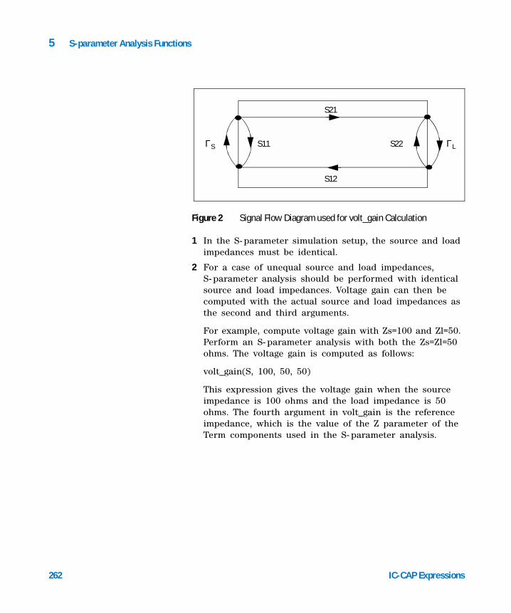
262 IC-CAP Expressions
5 S-parameter Analysis Functions
Figure 2 Signal Flow Diagram used for volt_gain Calculation
1 In the S- parameter simulation setup, the source and load impedances must be identical.
2 For a case of unequal source and load impedances, S- parameter analysis should be performed with identical source and load impedances. Voltage gain can then be computed with the actual source and load impedances as the second and third arguments.
For example, compute voltage gain with Zs=100 and Zl=50. Perform an S- parameter analysis with both the Zs=Zl=50 ohms. The voltage gain is computed as follows:
volt_gain(S, 100, 50, 50)
This expression gives the voltage gain when the source impedance is 100 ohms and the load impedance is 50 ohms. The fourth argument in volt_gain is the reference impedance, which is the value of the Z parameter of the Term components used in the S- parameter analysis.
S21
S12
S11 S22ΓS ΓL
S-parameter Analysis Functions 5
IC-CAP Expressions 263
volt_gain_max()
This measurement determines the ratio of the voltage across the load to the voltage available from the source at maximum power transfer. The network- parameter transformation function “stos()” on page 251 can be used to change the normalizing impedance of the scattering matrix.
Synopsis Y = volt_gain_max(S, Zs, Zl{, Zref})
where
S is the 2 × 2 scattering matrix.
Zs and Zl are the input and output impedances, respectively.
Zref is the reference impedance, set by default 50 ohms.
Examples vGain = volt_gain_max(S, 50, 75) - Zref defaults to 50 ohmsvGain1 = volt_gain(S, 50, 75, 75) - Zref = 75 ohms
Defined in $ICCAP_ROOT/expressions/ael/rf_system_fun.ael
See also “pwr_gain()” on page 236, “volt_gain()” on page 261

264 IC-CAP Expressions
5 S-parameter Analysis Functions
vswr()
Given a complex reflection coefficient, this measurement returns the voltage standing wave ratio.
Synopsis y = vswr(Sii)
where Sii is the complex reflection coefficient.
Examples a = vswr(S11)
Defined in $ICCAP_ROOT/expressions/ael/rf_system_fun.ael
See also “yin()” on page 267, “zin()” on page 273
S-parameter Analysis Functions 5
IC-CAP Expressions 265
write_snp()
Write S- Parameters in Touchstone SnP file format. Returns True or False.
Synopsis y = write_snp(FileName, Smatrix [, Comment, FreqUnit, DataFormat, Smatrix, Zref])
where
FileName is name or full- path of the S- Parameter file.
Smatrix is S- parameter matrix variable (1 to 99 ports)
Comment is text that is to be written at the top of file. Default is "".
FreqUnit is frequency unit – “Hz”, “KHz”, “MHz”, “GHz”, “THz”. Default is “GHz”.
DataFormat is format of S- Parameter that is to be output – “MA”, “DB”, “RI”. Default is “MA”.
Zref is reference impedance or value of R in the output file. Default is 50.0.
Examples This example assumes that an S- parameter Analysis has been performed, and the data is to be written to a file.writeTS = write_snp("spar_ts.s2p", S, "S-par simulation data", "GHz", "MA", 50)
writes the S- Parameters to the file spar_ts.s2p in mag- phase format
write_snp("spar_ts_1.s2p", S, "S-par simulation data")
writes the S- Parameters to the file spar_ts_1.s2p in default "GHz", mag- phase format and reference impedance of 50.0.
Used in S- Parameter Analysis.
Defined in $HPEESOF_DIR/expressions/ael/network_fun.ael
See also “stos()” on page 251
Notes/Equations
The function supports only 1- dimensional S- Parameter data. S- parameters can be from 1 to 99 ports. Z, Y, G and H parameters are not supported.

266 IC-CAP Expressions
5 S-parameter Analysis Functions
Function does not support writing noise data.
DataFormat can be set to one of the following:
• “MA”: magnitude- phase
• “DB”: dB- phase
• “RI”: real- imaginary

S-parameter Analysis Functions 5
IC-CAP Expressions 267
yin()
Given a reflection coefficient and the reference impedance, this measurement returns the input admittance looking into the measurement ports.
Synopsis y = yin(Sii, Z)
where
Sii is a complex reflection coefficient.
Z is a reference impedance.
Examples a = yin(S11, 50)
Defined in $ICCAP_ROOT/expressions/ael/network_fun.ael
See also “vswr()” on page 264, “zin()” on page 273
268 IC-CAP Expressions
5 S-parameter Analysis Functions
yopt()
Returns optimum admittance for noise match.
Synopsis y = yopt(gammaOpt, zRef)
where
gammaOpt is a optimum reflection coefficient.
zRef is a reference impedance.
Examples a = yopt(Sopt, 50)
Defined in Built in
See also “zopt()” on page 274
Notes/Equations
Used in Small- signal S- parameter simulations
This complex measurement produces the optimum source admittance for noise matching. gammaOpt is the optimum reflection coefficient that must be presented at the input of the network to realize the minimum noise figure (NFmin).

S-parameter Analysis Functions 5
IC-CAP Expressions 269
ytoabcd()
This measurement transforms an admittance matrix of a 2- port network into a hybrid matrix.
Synopsis z = ytoabcd(Y)
where Y is an admittance matrix.
Examples a = ytoabcd(Y)
Defined in $ICCAP_ROOT/expressions/ael/network_fun.ael
See also “abcdtoh()” on page 203, “htoabcd()” on page 219
270 IC-CAP Expressions
5 S-parameter Analysis Functions
ytoh()
This measurement transforms an admittance matrix of a 2- port network into a hybrid matrix.
Synopsis z = ytoh(Y)
where Y is an admittance matrix.
Examples h = ytoh(Y)
Defined in $ICCAP_ROOT/expressions/ael/network_fun.ael
See also “htoy()” on page 221, “ytoabcd()” on page 269
S-parameter Analysis Functions 5
IC-CAP Expressions 271
ytos()
This measurement transforms an admittance matrix into a scattering matrix.
Synopsis z = ytos(Y, zRef)
where
Y is an admittance matrix.
zRef is a reference impedance and can be an integer, real, or complex number.
Examples s = ytos(Y, 50.0)
Defined in $ICCAP_ROOT/expressions/ael/network_fun.ael
See also “stoy()” on page 253, “ytoz()” on page 272
272 IC-CAP Expressions
5 S-parameter Analysis Functions
ytoz()
This measurement transforms an admittance matrix to an impedance matrix.
Synopsis z = ytoz(Y)
where Y is an admittance matrix
Examples a = ytoz(Y)
Defined in $ICCAP_ROOT/expressions/ael/network_fun.ael
See also “ytos()” on page 271, “ztoy()” on page 278
S-parameter Analysis Functions 5
IC-CAP Expressions 273
zin()
Given a reflection coefficient and the reference impedance, this measurement returns the input impedance looking into the measurement ports.
Synopsis y = zin(Sii, Z)
where
Sii is a complex reflection coefficient.
Z is a reference impedance.
Examples a = zin(S11, 50.0)
Defined in $ICCAP_ROOT/expressions/ael/network_fun.ael
See also “vswr()” on page 264, “yin()” on page 267

274 IC-CAP Expressions
5 S-parameter Analysis Functions
zopt()
Returns the optimum impedance for noise matching.
Synopsis y = zopt(gammaOpt, zRef)
where
gammaOpt is an optimum reflection coefficient.
zRef is a reference impedance.
Examples a = zopt(Sopt, 50)
Defined in $ICCAP_ROOT/expressions/ael/circuit_fun.ael
See also “yopt()” on page 268
Notes/Equations
Used in Small- signal S- parameter simulations
This complex measurement produces the optimum source impedance for noise matching. gammaOpt is the optimum reflection coefficient that must be presented at the input of a network to realize the minimum noise figure (NFmin).

S-parameter Analysis Functions 5
IC-CAP Expressions 275
ztoabcd()
This measurement transforms an impedance matrix of a 2- port network into a chain (ABCD) matrix.
Synopsis y = ztoabcd(Z)
where Z is an impedance matrix.
Examples a = ztoabcd(Z)
Defined in $ICCAP_ROOT/expressions/ael/network_fun.ael
See also “abcdtoz()” on page 206, “ytoabcd()” on page 269, “ztoh()” on page 276

276 IC-CAP Expressions
5 S-parameter Analysis Functions
ztoh()
This measurement transforms an impedance matrix of a 2- port network into a hybrid matrix.
Synopsis y = ztoh(Z)
where Z is an impedance matrix.
Examples h = ztoh(Z)
Defined in $ICCAP_ROOT/expressions/ael/network_fun.ael
See also “htoz()” on page 222, “ytoh()” on page 270, “ztoabcd()” on page 275
S-parameter Analysis Functions 5
IC-CAP Expressions 277
ztos()
This measurement transforms an impedance matrix to a scattering matrix.
Synopsis y = ztos(Z, zRef)
where
Z is an impedance matrix.
zRef is a reference impedance and can be an integer, real, or complex number.
Examples s = ztos(Z, 50.0)
Defined in $ICCAP_ROOT/expressions/ael/network_fun.ael
See also “stoz()” on page 254, “ytoz()” on page 272, “ztoy()” on page 278

278 IC-CAP Expressions
5 S-parameter Analysis Functions
ztoy()
This measurement transforms an impedance matrix to an admittance matrix.
Synopsis y = ztoy(Z)
where Z is an impedance matrix.
Examples a = ztoy(Z)
Defined in $ICCAP_ROOT/expressions/ael/network_fun.ael
See also “stoz()” on page 254, “ytos()” on page 271, “ztoy()” on page 278

279
Agilent 85190A IC-CAP 2006Expressions
Agilent Technologies
6Statistical Analysis Functions
cdf() 280
cross_corr() 281
histogram() 282
histogram_multiDim() 284
histogram_sens() 285
histogram_stat() 286
lognorm_dist_inv1D() 287
lognorm_dist1D() 288
moving_average() 289
norm_dist_inv1D() 290
norm_dist1D() 291
norms_dist_inv1D() 292
norms_dist1D() 293
pdf() 294
stddev() 295
stddev_outer() 296
uniform_dist_inv1D() 297
uniform_dist1D() 298
yield_sens() 299
This chapter describes the statistical analysis functions in detail. The functions are listed in alphabetical order.
280 IC-CAP Expressions
6 Statistical Analysis Functions
cdf()
Returns the cumulative distribution function (CDF).
Synopsis y = cdf(data, numBins, minBin, maxBin)
where
data is the signal.
numBins is the number of subintervals or bins used to measure CDF. This is an optional value.
minBin and maxBin are the beginning and end, respectively, of the evaluation of the CDF. These are optional values.
Examples y = cdf(data)y = cdf(data, 20)
Defined in $ICCAP_ROOT/expressions/ael/statistical_fun.ael
See also “histogram()” on page 282, “pdf()” on page 294, “yield_sens()” on page 299
Notes/Equations
This function measures the cumulative distribution function of a signal. The default values for minBin and maxBin are the minimum and the maximum values of the data, and numBins is set to log(numOfPts)/log(2.0) by default.
This function can only be used by entering an equation (Eqn) in the Data Display window.

Statistical Analysis Functions 6
IC-CAP Expressions 281
cross_corr()
Returns the cross- correlation.
Synopsis cross_corr(v1, v2)
where v1 and v2 are 1- dimensional data
Examples v1 = qpsk..videal[1]v2 = qpsk..vout[1]x_corr_v1v2 = cross_corr(v1, v2)auto_corr_v1 = cross_corr(v1, v1)
Defined in $ICCAP_ROOT/expressions/ael/digital_wireless_fun.ael
282 IC-CAP Expressions
6 Statistical Analysis Functions
histogram()
Generates a histogram representation. This function creates a histogram that represents data.
Synopsis y = histogram(data, numBins, minBin, maxBin)
where
data is the signal and must be one- dimensional.
numBins is number of subintervals or bins used to measure the histogram. numBins is set to log(numOfPts)/log(2.0) by default.
minBin and maxBin are the beginning and end, respectively, of the evaluation of the histogram. The default values for minBin and maxBin are the minimum and the maximum values, respectively, of the data.
Examples y = histogram(data)y = histogram(data, 20)
If you have performed a parameter sweep such that the first argument (data) in the histogram function is a function of two independent variables, then you must reduce the dimensionality of data before using it in the histogram function. For example, if you run a Monte Carlo simulation on the S- parameters of a circuit, S21 would be a function of both the Monte Carlo index and the frequency (assuming you have swept frequency). So, you could plot the histogram of S21 at the 100th frequency in the sweep by using:
y = histogram(dB(S21[::,99]))
See also $ICCAP_ROOT/examples/Tutorial/yldex1_prj(see measurement_hist.dds and worstcase_measurement_hist.dds)
Defined in Built in
See also “cdf()” on page 280, “pdf()” on page 294, “yield_sens()” on page 299, “histogram_multiDim()” on page 284, “histogram_stat()” on page 286

Statistical Analysis Functions 6
IC-CAP Expressions 283
Notes/Equations
This function can only be used by entering an equation (Eqn) in the Data Display window.
284 IC-CAP Expressions
6 Statistical Analysis Functions
histogram_multiDim()
Collapses the multi- dimensional data down to one- dimensional data and applies the histogram to the one- dimensional data.
Synopsis y = histogram_multiDim(data{, normalized, numBins, minBin, maxBin})
where
data is the signal.
When normalized is set to "yes", the histogram is generated with percent on the Y- axis instead of the number of outcomes.
numBins is number of subintervals or bins used to measure the histogram.
minBin and maxBin are the beginning and end, respectively, of the evaluation of the histogram.
Examples Given monte carlo analysis results for the S12. It is two- dimensional data: the outer sweep is mcTrial; the inner sweep is the frequency from 100 MHz to 500 MHz.Histogram_multiDim_S12 = histogram_multiDim(S12)
See also $ICCAP_ROOT/examples/Tutorial/yldex1_prj(see measurement_hist.dds and worstcase_measurement_hist.dds)
Defined in $ICCAP_ROOT/expressions/ael/statistical_fun.ael
See also “collapse()” on page 43, “histogram()” on page 282
NOTE This function calls the collapse() function, therefore, it only works for data with dimension less than four.
Statistical Analysis Functions 6
IC-CAP Expressions 285
histogram_sens()
Produces the yield sensitivity histogram displaying the sensitivity of a measurement statistical response to a selected statistical variable. The function is mainly applied to the statistical analysis (Monte Carlo/Yield/YieldOpt) results.
Synopsis y = histogram_sens(data, sensitivityVar{, goalMin, goalMax, innermostIndepLow, innermostIndepHigh, numBins})
where
data is the statistical response.
sensitivityVar is the selected statistical variable.
goalMin and goalMax specifies the performance range - the yield is 1 inside the range, and the yield is zero outside the range. Note that while goalMin and goalMax are optional arguments, at least one of them must be specified.
innermostIndepLow and innermostIndepHigh specifies the subrange of data with the inner most sweep variable.
numBins is number of subintervals or bins used to measure the histogram.
Examples Given monte carlo analysis results for the S11. It is two- dimensional data: the outer sweep is mcTrial; the inner sweep is the frequency from 100 MHz to 500 MHz.
The design wants the maximum of db(S11) is - 18.0dB in the frequency range of 200 MHz to 400 MHz. The yield sensitivity of such performance to statistical variable "C1v" can be calculated as:Histogram_sens_S11 = histogram_sens(dB(S11),C1v,,-18.0,200MHz,400MHz)
Defined in $ICCAP_ROOT/expressions/ael/statistical_fun.ael
See also “histogram()” on page 282, “histogram_multiDim()” on page 284, “histogram_stat()” on page 286, “build_subrange()” on page 39, “yield_sens()” on page 299

286 IC-CAP Expressions
6 Statistical Analysis Functions
histogram_stat()
Produces the histogram of a subrange of the multi- dimension data. It first calls build_subrange() to build the subrange of a mulit- dimension data, then calls histogram_multiDim() to produce the histogram.
Synopsis y = histogram_stat(data{, normalized, innermostIndepLow, innermostIndepHigh, numBins, minBin, maxBin})
where
data is the statistical analysis.
When normalized is set to "yes", the histogram is generated with percent on the Y- axis instead of the number of outcomes.
innermostIndepLow and innermostIndepHigh specifies the subrange of data with the inner most sweep variable.
numBins is number of subintervals or bins used to measure the histogram.
minBin and maxBin are the beginning and end, respectively, of the evaluation of the histogram.
Examples Given monte carlo analysis results for the S12. It is two- dimensional data: the outer sweep is mcTrial; the inner sweep is the frequency from 100 MHz to 500 MHz.Histogram_stat_S12 = histogram_stat(S12,,200MHz,400MHz)
Defined in $ICCAP_ROOT/expressions/ael/statistical_fun.ael
See also “histogram()” on page 282, “histogram_multiDim()” on page 284, “build_subrange()” on page 39
NOTE Because this function calls the histogram_multi() function, which calls the collapse() function, it is only valid for data with dimension less than four.

Statistical Analysis Functions 6
IC-CAP Expressions 287
lognorm_dist_inv1D()
Returns the inverse of the cumulative distribution function (cdf) for a lognormal distribution.
Synopsis y = lognorm_dist_inv1D(data, m, s{, absS})
where
data is a real number in range [0,1] representing the cumulative probability.
m and s are the mean and standard deviation for the lognormal distribution. Can an integer or real number.
When absS is not equal to "0", s is the absolute standard deviation; otherwise, s is the relative standard deviation. Must be an integer and the default is "1".
Examples X_cpf = 0.5X= lognorm_dist_inv1D(X_cpf, 2.0, 0.2, 1)XX_cpf=[0.0::0.01::1.0]XX= lognorm_dist_inv1D(XX_cpf, 2.0, 0.2, 1)
Defined in $ICCAP_ROOT/expressions/ael/statistical_fun.ael
288 IC-CAP Expressions
6 Statistical Analysis Functions
lognorm_dist1D()
Returns a lognormal distribution: either its probability density function (pdf), or cumulative distribution function (cdf).
Synopsis y = lognorm_dist1D(data, m, s{, absS, is_cpf})
where
data is a number or a one- dimensional data.
m and s are the mean and standard deviation for the lognormal distribution. Can an integer or real number.
When absS is not equal to "0", the given "s" represents the absolute standard deviation value; otherwise, "s" is the relative standard deviation. Must be an integer and the default is "1".
is_cdf is required as an integer number. When is_cdf is not equal to "0", the function returns the cdf of the lognormal distribution. Otherwise, it returns the pdf of the lognormal distribution. Default is "0".
Examples X = 0.5X_pdf= lognorm_dist1D(X, 2.0,0.2, 1, 0)X_cdf = lognorm_dist1D(X,2.0,0.1, 0, 1)XX=[-3.9::0.1::3.9]XX_pdf = lognorm_dist1D(XX,2.0, 0.2,1,0)XX_cdf = lognorm_dist1D(XX,2.0,0.2,0,1)
Defined in $ICCAP_ROOT/expressions/ael/statistical_fun.ael

Statistical Analysis Functions 6
IC-CAP Expressions 289
moving_average()
Returns the moving_average of a sequence of data.
Synopsis y = moving_average(data, numPoints)
where
data is a one- dimensional sequence of numbers in brackets “[x, y, ...]”.
numPoints is the number of points to be averaged together. (see notes section)
Examples a = moving_average([1, 2, 3, 7, 5, 6, 10], 3)
returns [1, 2, 4, 5, 6, 7, 10]
Built in $ICCAP_ROOT/expressions/ael/statistcal_fun.ael
Notes/Equations
numPoints must be an odd number. If even, the value is increased to the next odd number. If greater or equal to the number of data points, the value is set to number of data points - 1 for even number of data points. For odd number of data points, numPoints is set to number of data points.
The first value of the smoothed sequence is the same as the original data. The second value is the average of the first three. The third value is the average of data elements 2, 3, and 4, etc. If numPoints were set to 7, for example, then the first value of the smoothed sequence would be the same as the original data. The second value would be the average of the first three original data points. The third value would be the average of the first five data points, and the fourth value would be the average of the first seven data points. Subsequent values in the smoothed array would be the average of the seven closest neighbors. The last points in the smoothed sequence are computed in a way similar to the first few points. The last point is just the last point in the original sequence. The second from last point is the average of the last three points in the original sequence. The third from the last point is the average of the last five points in the original sequence, etc.

290 IC-CAP Expressions
6 Statistical Analysis Functions
norm_dist_inv1D()
Returns the inverse of the cumulative distribution function (cdf) for a normal distribution.
Synopsis y = norm_dist_inv1D(data, m, s{, absS})
where
data is a real number in range [0,1] representing the cumulative probability.
m and s are the mean and standard deviation of the normal distribution. Can be an integer or real number.
When absS is not equal to "0", s is the absolute standard deviation; otherwise, s is the relative standard deviation. Default is "1".
Examples X_cpf = 0.5X= norm_dist_inv1D(X_cpf, 0, 1, 1)
will be equal to 0.0XX_cpf=[0.0::0.01::1.0]XX= norm_dist_inv1D(XX_cpf, 5.0, 0.5, 1)
Defined in $ICCAP_ROOT/expressions/ael/statistical_fun.ael
See also “norm_dist1D()” on page 291, “norms_dist_inv1D()” on page 292, “norms_dist1D()” on page 293, “lognorm_dist_inv1D()” on page 287, “lognorm_dist1D()” on page 288, “uniform_dist_inv1D()” on page 297, “uniform_dist1D()” on page 298

Statistical Analysis Functions 6
IC-CAP Expressions 291
norm_dist1D()
Returns a normal distribution: either its probability density function (pdf), or cumulative distribution function (cdf).
Synopsis y = norm_dist1D(data, m, s{, absS, is_cpf})
where
data is a number or a one- dimensional data.
m and s are the mean and standard deviation for the normal distribution. Can be an integer or real number.
When absS is not equal to "0", the given "s" represents the absolute standard deviation value; otherwise, "s" is the relative standard deviation. Must be an integer and default is "1".
is_cdf is required as an integer number. When is_cdf is not equal to "0", the function returns the cdf of the normal distribution. Otherwise, it returns the pdf of the normal distribution. Default is "0".
Examples X = 0.5X_pdf= norm_dist1D(X, 0, 1, 1, 0)X_cdf = norm_dist1D(X,0, 1, 1, 1)XX=[-3.9::0.1::3.9]XX_pdf = norm_dist1D(XX,5.0, 0.5,1,0)XX_cdf = norm_dist1D(XX,5.0,0.1,0,1)
Defined in $ICCAP_ROOT/expressions/ael/statistical_fun.ael
See also “norm_dist_inv1D()” on page 290, “norms_dist_inv1D()” on page 292, “norms_dist1D()” on page 293, “lognorm_dist_inv1D()” on page 287, “lognorm_dist1D()” on page 288, “uniform_dist_inv1D()” on page 297, “uniform_dist1D()” on page 298
292 IC-CAP Expressions
6 Statistical Analysis Functions
norms_dist_inv1D()
Returns the inverse of the cumulative distribution function (cdf) for a standard normal distribution.
Synopsis y = norms_dist_inv1D(data)
where
data is an integer or real number in range [0,1] representing the cumulative probability.
Examples X_cpf = 0.5X= norms_dist_inv1D(X_cpf)
will be equal to 0.0XX_cpf=[0.0::0.01::1.0]XX= norms_dist_inv1D(XX_cpf)
Defined in $ICCAP_ROOT/expressions/ael/statistical_fun.ael
See also “norm_dist1D()” on page 291, “norm_dist_inv1D()” on page 290, “norms_dist1D()” on page 293, “lognorm_dist_inv1D()” on page 287, “lognorm_dist1D()” on page 288, “uniform_dist_inv1D()” on page 297, “uniform_dist1D()” on page 298
Statistical Analysis Functions 6
IC-CAP Expressions 293
norms_dist1D()
Returns the standard normal distribution: either its probability density function (pdf), or cumulative distribution function (cdf).
Synopsis y = norms_dist1D(data{, is_cdf})
where
data is a number or a one- dimensional data.
is_cdf is required as an integer number. When is_cdf is not equal to "0", the function returns the cdf of the standard normal distribution. Otherwise, it returns the pdf of the standard normal distribution. Default is "0".
Examples X = 0.5X_pdf= norms_dist1D(X, 0)X_cdf = norms_dist1D(X,1)XX=[-3.9::0.1::3.9]XX_pdf = norms_dist1D(XX,0)XX_cdf = norms_dist1D(XX,1)
Defined in $ICCAP_ROOT/expressions/ael/statistical_fun.ael
See also “norm_dist1D()” on page 291, “norm_dist_inv1D()” on page 290, “norms_dist_inv1D()” on page 292, “lognorm_dist_inv1D()” on page 287, “lognorm_dist1D()” on page 288, “uniform_dist_inv1D()” on page 297, “uniform_dist1D()” on page 298

294 IC-CAP Expressions
6 Statistical Analysis Functions
pdf()
Returns a probability density function (PDF).
Synopsis y = pdf(x, numBins, minBin, maxBin)
where
x is the signal.
numBins is number of subintervals or bins used to measure PDF.
minBin and maxBin are the beginning and end, respectively, of the evaluation of the PDF.
Examples y = pdf(data)y = pdf(data, 20)
Defined in AEL statistical_fun.ael
See also “cdf()” on page 280, “histogram()” on page 282, “yield_sens()” on page 299
Notes/Equations
This function measures the probability density function of a signal. The default values for minBin and maxBin are the minimum and the maximum values of the data and numBins is set to log(numOfPts)/log(2.0) by default.
This function can only be used by entering an equation (Eqn) in the Data Display window.

Statistical Analysis Functions 6
IC-CAP Expressions 295
stddev()
The stddev() function calculates the standard deviation of the data.
Synopsis y = stddev(x{, flag})
where
x is the data.
flag is used to indicate how stddev normalizes. By default, flag is set to 0, which means that stddev normalizes by N- 1, where N is the length of the data sequence. Otherwise, stddev normalizes by N.
Examples a = stddev(data)a = stddev(data, 1)
Defined in $ICCAP_ROOT/expressions/ael/statistical_fun.ael
See also “mean()” on page 167
Notes/Equations
This function can only be used by entering an equation (Eqn) in the Data Display window.
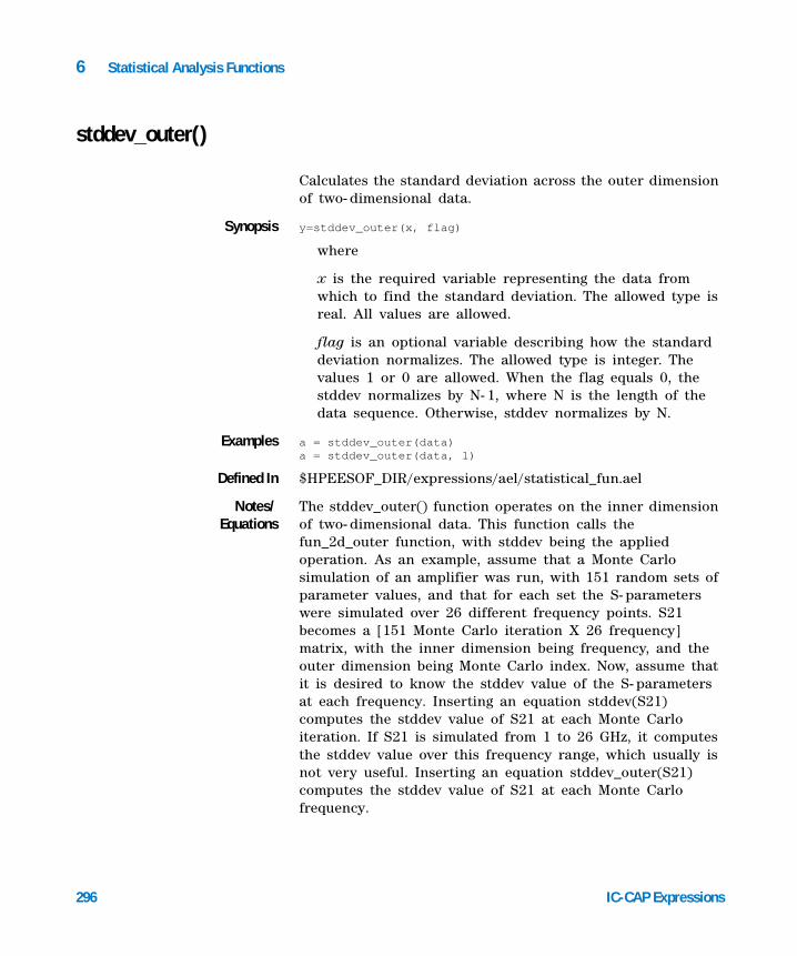
296 IC-CAP Expressions
6 Statistical Analysis Functions
stddev_outer()
Calculates the standard deviation across the outer dimension of two- dimensional data.
Synopsis y=stddev_outer(x, flag)
where
x is the required variable representing the data from which to find the standard deviation. The allowed type is real. All values are allowed.
flag is an optional variable describing how the standard deviation normalizes. The allowed type is integer. The values 1 or 0 are allowed. When the flag equals 0, the stddev normalizes by N- 1, where N is the length of the data sequence. Otherwise, stddev normalizes by N.
Examples a = stddev_outer(data)a = stddev_outer(data, 1)
Defined In $HPEESOF_DIR/expressions/ael/statistical_fun.ael
Notes/Equations
The stddev_outer() function operates on the inner dimension of two- dimensional data. This function calls the fun_2d_outer function, with stddev being the applied operation. As an example, assume that a Monte Carlo simulation of an amplifier was run, with 151 random sets of parameter values, and that for each set the S- parameters were simulated over 26 different frequency points. S21 becomes a [151 Monte Carlo iteration X 26 frequency] matrix, with the inner dimension being frequency, and the outer dimension being Monte Carlo index. Now, assume that it is desired to know the stddev value of the S- parameters at each frequency. Inserting an equation stddev(S21) computes the stddev value of S21 at each Monte Carlo iteration. If S21 is simulated from 1 to 26 GHz, it computes the stddev value over this frequency range, which usually is not very useful. Inserting an equation stddev_outer(S21) computes the stddev value of S21 at each Monte Carlo frequency.
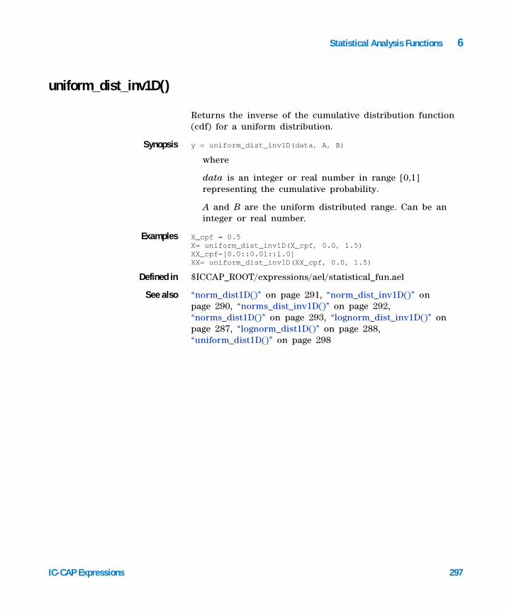
Statistical Analysis Functions 6
IC-CAP Expressions 297
uniform_dist_inv1D()
Returns the inverse of the cumulative distribution function (cdf) for a uniform distribution.
Synopsis y = uniform_dist_inv1D(data, A, B)
where
data is an integer or real number in range [0,1] representing the cumulative probability.
A and B are the uniform distributed range. Can be an integer or real number.
Examples X_cpf = 0.5X= uniform_dist_inv1D(X_cpf, 0.0, 1.5)XX_cpf=[0.0::0.01::1.0]XX= uniform_dist_inv1D(XX_cpf, 0.0, 1.5)
Defined in $ICCAP_ROOT/expressions/ael/statistical_fun.ael
See also “norm_dist1D()” on page 291, “norm_dist_inv1D()” on page 290, “norms_dist_inv1D()” on page 292, “norms_dist1D()” on page 293, “lognorm_dist_inv1D()” on page 287, “lognorm_dist1D()” on page 288, “uniform_dist1D()” on page 298

298 IC-CAP Expressions
6 Statistical Analysis Functions
uniform_dist1D()
Returns a uniform distribution: either its probability density function (pdf), or cumulative distribution function (cdf).
Synopsis y = uniform_dist1D(data, A, B{, is_cpf})
where
data is a number or a one- dimensional data. Can be an integer or real number.
A and B are the uniform distributed range. Can be an integer or real number.
is_cdf is required as an integer number. When is_cdf is not equal to "0", the function returns the cdf of the uniform distribution. Otherwise, it returns the pdf of the uniform distribution. Default is "0".
Examples X = 0.5X_pdf= uniform_dist1D(X, 0.0,1.0, 0)X_cdf = uniform_dist1D(X,0.0,1.0, 1)XX=[-3.9::0.1::3.9]XX_pdf = uniform_dist1D(XX,0.0,5.0,0)XX_cdf = uniform_dist1D(XX,0.0,5.0,1)
Defined in $ICCAP_ROOT/expressions/ael/statistical_fun.ael
See also “norm_dist1D()” on page 291, “norm_dist_inv1D()” on page 290, “norms_dist_inv1D()” on page 292, “norms_dist1D()” on page 293, “lognorm_dist_inv1D()” on page 287, “lognorm_dist1D()” on page 288, “uniform_dist_inv1D()” on page 297

Statistical Analysis Functions 6
IC-CAP Expressions 299
yield_sens()
Returns the yield as a function of a design variable.
Synopsis y = yield_sens(pf_data{, numBins})
where
pf_data is a binary- valued scalar data set indicating the pass/fail status of each value of a companion independent variable.
numBins is the number of subintervals or bins used to measure yield_sens.
Examples a = yield_sens(pf_data)a = yield_sens(pf_data, 20)
Defined in $ICCAP_ROOT/expressions/ael/statistical_fun.ael
See also “cdf()” on page 280, “histogram()” on page 282, “pdf()” on page 294
Notes/Equations
Used in Monte Carlo simulation.
This function measures the yield as a function of a design variable. The default value for numBins is set to log(numOfPts)/log(2.0) by default. For more information and an example refer to "Creating a Sensitivity Histogram" in the "Tuning, Optimization and Statistical Design" documentation.
This function can only be used by entering an equation (Eqn) in the Data Display window.

300 IC-CAP Expressions
6 Statistical Analysis Functions

301
Agilent 85190A IC-CAP 2006Expressions
Agilent Technologies
7Transient Analysis Functions
Working with Transient Data 302
constellation() 303
cross() 305
fspot() 306
ifc_tran() 309
ispec_tran() 310
pfc_tran() 311
pspec_tran() 312
pt_tran() 313
step() 314
vfc_tran() 315
vspec_tran() 316
vt_tran() 317
This chapter describes the transient analysis functions in detail. The functions are listed in alphabetical order.

302 IC-CAP Expressions
7 Transient Analysis Functions
Working with Transient Data
Transient analysis produces real voltages and currents as a function of time. A single analysis produces 1- dimensional data. Sections of time- domain waveforms can be indexed by using a sequence within “[ ]”.

Transient Analysis Functions 7
IC-CAP Expressions 303
constellation()
Generates the constellation diagram from Circuit Envelope, Transient, or Ptolemy simulation I and Q data.
Synopsis Const = constellation(i_data, q_data, symbol_rate, delay)
where
i_data is the in- phase component of data versus time of a single complex voltage spectral component (for example, the fundamental) (this could be a baseband signal instead, but in either case it must be real- valued versus time).
q_data is the quadrature- phase component of data versus time of a single complex voltage spectral component (for example, the fundamental) (this could be a baseband signal instead, but in either case it must be real valued versus time).
symbol_rate is the symbol rate of the modulation signal.
delay (if nonzero) throws away the first delay = N seconds of data from the constellation plot. It is also used to interpolate between simulation time points, which is necessary if the optimal symbol- sampling instant is not exactly at a simulation time point. Usually this parameter must be nonzero to generate a constellation diagram with the smallest grouping of sample points.
Examples Rotation = −0.21Vfund =vOut[1] ⋅ exp(j ⋅ Rotation)delay =1/sym_rate[0, 0] − 0.5 ⋅ tstep[0, 0]Vimag = imag(Vfund)Vreal = real(Vfund)Const = constellation(Vreal, Vimag, sym_rate[0, 0], delay)
where Rotation is a user- selectable parameter that rotates the constellation by that many radians, and vOut is the named connection at a node. The parameter delay can be a numeric value, or in this case an equation using sym_rate, the symbol rate of the modulated signal, and tstep, the time step of the simulation. If these equations are to be used in a Data Display window, sym_rate and tstep must be defined by means of a variable (VAR)
304 IC-CAP Expressions
7 Transient Analysis Functions
component, and they must be passed into the dataset as follows: Make the parameter Other visible on the Envelope simulation component, and edit it so that
Other = OutVar = sym_rate OutVar = tstep
In some cases, it may be necessary to experiment with the value of delay to get the constellation diagram with the tightest points.
Defined in $ICCAP_ROOT/expressions/ael/digital_wireless_fun.ael
Notes/Equations
Used in Constellation diagram generation.
The I and Q data do not need to be baseband waveforms. For example, they could be the in- phase (real or I) and quadrature- phase (imaginary or Q) part of a modulated carrier. The user must supply the I and Q waveforms versus time, as well as the symbol rate. A delay parameter is optional.
NOTE vOut is a named connection on the schematic. Assuming that a Circuit Envelope simulation was run, vOut is output to the dataset as a two-dimensional matrix. The first dimension is time, and there is a value for each time point in the simulation. The second dimension is frequency, and there is a value for each fundamental frequency, each harmonic, and each mixing term in the analysis, as well as the baseband term.
vOut[1] is the equivalent of vOut[::, 1], and specifies all time points at the lowest non-baseband frequency (the fundamental analysis frequency, unless a multitone analysis has been run and there are mixing products).
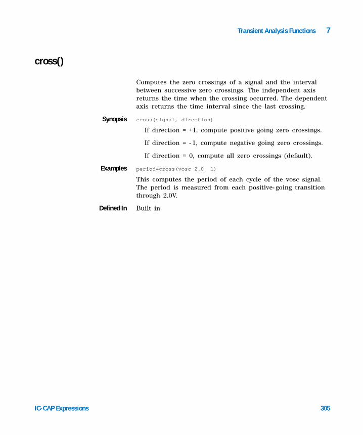
Transient Analysis Functions 7
IC-CAP Expressions 305
cross()
Computes the zero crossings of a signal and the interval between successive zero crossings. The independent axis returns the time when the crossing occurred. The dependent axis returns the time interval since the last crossing.
Synopsis cross(signal, direction)
If direction = +1, compute positive going zero crossings.
If direction = - 1, compute negative going zero crossings.
If direction = 0, compute all zero crossings (default).
Examples period=cross(vosc-2.0, 1)
This computes the period of each cycle of the vosc signal. The period is measured from each positive- going transition through 2.0V.
Defined In Built in

306 IC-CAP Expressions
7 Transient Analysis Functions
fspot()
Performs a single- frequency time- to- frequency transform.
Synopsis fspot(x{, fund, harm, windowType, windowConst, interpOrder, tstart})
See detailed Notes/ Equations below.
Examples The following example equations assume that a transient simulation was performed from 0 to 5 ns on a 1- GHz- plus- harmonics signal called vOut:fspot(vOut)
returns the 200- MHz component, integrated from 0 to 5 ns.
fspot(vOut, , 5)
returns the 1- GHz component, integrated from 0 to 5 ns.fspot(vOut, 1GHz, 1)
returns the 1- GHz component, integrated from 4 to 5 ns.fspot(vOut, 0.5GHz, 2, , , , 2.5ns)
returns the 1- GHz component, integrated from 2.5 to 4.5 ns.
fspot(vOut, 0.25GHz, 4, "Kaiser")
returns the 1- GHz component, integrated from 1 to 5 ns, after applying the default Kaiser window to this range of data.
fspot(vOut, 0.25GHz, 4, 3, 2.0)
returns the 1- GHz component, integrated from 1 to 5 ns, after applying a Gaussian window with a constant of 2.0 to this range of data.
Defined in Built in
See also “fft()” on page 145
Notes/Equations
fspot(x) returns the discrete Fourier transform of the vector x evaluated at one specific frequency. The value returned is the peak component, and it is complex. The harmth harmonic of the fundamental frequency fund is obtained
Transient Analysis Functions 7
IC-CAP Expressions 307
from the vector x. The Fourier transform is applied from time tstop–1/fund to tstop, where tstop is the last timepoint in x.
When x is a multidimensional vector, the transform is evaluated for each vector in the specified dimension. For example, if x is a matrix, then fspot(x) applies the transform to every row of the matrix. If x is three dimensional, then fspot(x) is applied in the lowest dimension over the remaining two dimensions. The dimension over which to apply the transform may be specified by dim; the default is the lowest dimension (dim=1). x must be numeric. It will typically be data from a transient, signal processing, or envelope analysis.
fund must be greater than zero. It is used to specify the period 1/fund for the Fourier transform. fund defaults to a period that matches the length of the independent axis of x.
harm may be any positive number. harm defaults to 1. Specifying harm=0 will compute the DC component of x.
The data to be transformed may be windowed. The window is specified by windowType, with an optional window constant windowConst. The window types and their default constants are:
0 = None
1 = Hamming 0.54
2 = Hanning 0.50
3 = Gaussian 0.75
4 = Kaiser 7.865
5 = 8510 6.0
6 = Blackman
7 = Blackman- Harris
windowType can be specified either by the number or by the name.
308 IC-CAP Expressions
7 Transient Analysis Functions
By default, the transform is performed at the end of the data from tstop- 1/fund to tstop. By using tstart, the transform can be started at some other point in the data. The transform will then be performed from tstart to tstart+1/fund.
Unlike with fft or fs, the data to be transformed are not zero padded or resampled. fspot works directly on the data as specified, including nonuniformly sampled data from a transient simulation.
Transient simulation uses a variable timestep and variable order algorithm. The user sets an upper limit on the allowed timestep, but the simulator will control the timestep so the local truncation error of the integration is controlled. If the Gear integration algorithm is used, the order can also be changed during simulation. fspot can use all of this information when performing the Fourier transform. The time data are not resampled; the Fourier integration is performed from timestep to timestep of the original data.
When the order varies, the Fourier integration will adjust the order of the polynomial it uses to compute the shape of the data between timepoints.
This variable order integration depends on the presence of a special dependent variable, tranorder, which is output by the transient simulator. If this variable is not present, or if the user wishes to override the interpolation scheme, then interpOrder may be set to a nonzero value:
1 = use only linear interpolation
2 = use quadratic interpolation
3 = use cubic polynomial interpolation
Only polynomials of degree one to three are supported. The polynomial is fit because time domain data are obtained by integrating forward from zero; previous data are used to determine future data, but future data can never be used to modify past data.
Transient Analysis Functions 7
IC-CAP Expressions 309
ifc_tran()
Returns frequency- selective current in Transient analysis.
Synopsis y = ifc_tran(iOut, fundFreq, harmNum)
where
iOut is the current through a branch.
fundFreq is the fundamental frequency.
harmNum is the harmonic number of the fundamental frequency (positive integer value only).
Examples y = ifc_tran(I_Probe1.i, 1GHz, 1)
Defined in $ICCAP_ROOT/expressions/ael/circuit_fun.ael
See also “pfc_tran()” on page 311, “vfc_tran()” on page 315
Notes/Equations
This measurement gives RMS current, in current units, for a specified branch at a particular frequency of interest. fundFreq determines the portion of the time- domain waveform to be converted to the frequency domain. This is typically one full period corresponding to the lowest frequency in the waveform. harmNum is the harmonic number of the fundamental frequency at which the current is requested.
310 IC-CAP Expressions
7 Transient Analysis Functions
ispec_tran()
Returns current spectrum.
Synopsis y = ispec_tran(iOut, fundFreq, numHarm)
where
iOut is the current through a branch.
fundFreq is the fundamental frequency value.
numHarm is the number of harmonics of fundamental frequency (positive integer value only).
Examples y = ispec_tran(I_Probe1.i, 1GHz, 8)
Defined in $ICCAP_ROOT/expressions/ael/circuit_fun.ael
See also “pspec_tran()” on page 312, “vspec_tran()” on page 316
Notes/Equations
This measurement gives a current spectrum for a specified branch. The measurement gives a set of RMS current values at each frequency. fundFreq determines the portion of the time- domain waveform to be converted to frequency domain. This is typically one full period corresponding to the lowest frequency in the waveform. numHarm is the number of harmonics of fundamental frequency to be included in the currents spectrum.

Transient Analysis Functions 7
IC-CAP Expressions 311
pfc_tran()
Returns frequency- selective power.
Synopsis y = pfc_tran(vPlus, vMinus, iOut, fundFreq, harmNum)
where
vPlus and vMinus are the voltages at the positive terminals.
iOut is the current through a branch measured for power calculation.
fundFreq is fundamental frequency.
harmNum is the harmonic number of the fundamental frequency (positive integer value only).
Examples a = pfc_tran(v1, v2, I_Probe1.i, 1GHz, 1)
Defined in $ICCAP_ROOT/expressions/ael/circuit_fun.ael
See also “ifc_tran()” on page 309, “vfc_tran()” on page 315
Notes/Equations
This measurement gives RMS power, delivered to any part of the circuit at a particular frequency of interest. fundFreq determines the portion of the time- domain waveform to be converted to frequency domain. This is typically one full period corresponding to the lowest frequency in the waveform. harmNum is the harmonic number of the fundamental frequency at which the power is requested.

312 IC-CAP Expressions
7 Transient Analysis Functions
pspec_tran()
Returns transient power spectrum.
Synopsis y = pspec_tran(vPlus, vMinus, iOut, fundFreq, numHarm)
where
vPlus and vMinus are the voltages at the positive and negative terminals.
iOut is the current through a branch measured for power calculation.
fundFreq is the fundamental frequency.
numHarm is the number of harmonics of the fundamental frequency (positive integer value only).
Examples a = pspec_tran(v1, v2, I_Probe1.i, 1GHz, 8)
Defined in $ICCAP_ROOT/expressions/ael/circuit_fun.ael
See also “ispec_tran()” on page 310, “vspec_tran()” on page 316
Notes/Equations
This measurement gives a power spectrum, delivered to any part of the circuit. The measurement gives a set of RMS power values at each frequency. fundFreq is the fundamental frequency determines the portion of the time- domain waveform to be converted to frequency domain (typically one full period corresponding to the lowest frequency in the waveform). numHarm is the number of harmonics of the fundamental frequency to be included in the power spectrum.

Transient Analysis Functions 7
IC-CAP Expressions 313
pt_tran()
Produces a transient time- domain power waveform for specified nodes.
Synopsis y=pt(vPlus, vMinus, current, fundFreq)
where
vPlus is a required variable representing the voltage at the positive terminal. The allowed types are real and complex. All values are allowed.
vMinus is a required variable representing the voltage at the negative terminal. The allowed types are real and complex. All values are allowed.
current is a required variable representing the current. The allowed types are real and complex. All values are allowed.
fundFreq is a required variable representing the fundamental frequency. Real is the only allowed value type. All positive values from 0 toward infinity are allowed.
Examples a = pt_tran(v1, v2, i1, 1GHz)
Defined In $HPEESOF_DIR/expressions/ael/circuit_fun.ael
See also “vt()” on page 104, “vt_tran()” on page 317
Notes/Equations
DC- to- RF efficiency is based on HB analysis.
314 IC-CAP Expressions
7 Transient Analysis Functions
step()
A step function that returns 0, 5, or 1. Returns: 0 if the argument < 0, .5 if argument == 0, or 1 if the argument > 0.
Synopsis y= step(x)
where x is any integer, real, or complex number.
Examples a = step(-1.5)
returns 0.000a = step(0)
returns 0.500a = step(1.5)
returns 1.000
Defined in built in

Transient Analysis Functions 7
IC-CAP Expressions 315
vfc_tran()
Returns the transient frequency- selective voltage.
Synopsis y = vfc_tran(vPlus, vMinus, fundFreq, harmNum)
where
vPlus and vMinus are the voltages at the positive and negative terminals.
fundFreq is the fundamental frequency.
harmNum is the harmonic number of the fundamental.
Examples a = vfc_tran(vOut, 0, 1GHz, 1)
Defined in $ICCAP_ROOT/expressions/ael/circuit_fun.ael
See also “ifc_tran()” on page 309, “pfc_tran()” on page 311
Notes/Equations
This measurement gives the RMS voltage across any two nodes at a particular frequency of interest. The fundamental frequency determines the portion of the time- domain waveform to be converted to frequency domain. This is typically one full period corresponding to the lowest frequency in the waveform. The harmonic number is the fundamental frequency at which the voltage is requested (positive integer value only).
316 IC-CAP Expressions
7 Transient Analysis Functions
vspec_tran()
Returns the transient voltage spectrum.
Synopsis y = vspec_tran(vPlus, vMinus, fundFreq, numHarm)
where
vPlus and vMinus are the voltages at the positive and negative terminals.
fundFreq is the fundamental frequency.
numHarm is the number of harmonics of the fundamental frequency (positive integer value only).
Examples a = vspec_tran(v1, v2, 1GHz, 8)
Defined in $ICCAP_ROOT/expressions/ael/circuit_fun.ael
See also “ispec_tran()” on page 310, “pspec_tran()” on page 312
Notes/Equations
This measurement gives a voltage spectrum across any two nodes. The measurement gives a set of RMS voltages at each frequency. The fundamental frequency determines the portion of the time- domain waveform to be converted to the frequency domain. This is typically one full period corresponding to the lowest frequency in the waveform. numHarm is the number of harmonics of the fundamental frequency to be included in the voltage spectrum.

Transient Analysis Functions 7
IC-CAP Expressions 317
vt_tran()
This measurement produces a transient time- domain voltage waveform for specified nodes. vPlus and vMinus are the nodes across which the voltage is measured.
Synopsis y = vt_tran(vPlus, vMinus)
where vPlus and vMinus are the terminals across which the voltage is measured.
Examples a = vt_tran(v1, v2)
Defined in $ICCAP_ROOT/expressions/ael/circuit_fun.ael
See also “vt()” on page 104

318 IC-CAP Expressions
7 Transient Analysis Functions
IC-CAP Expressions 319
Index
Aabcdtoh, 203abcdtos, 204abcdtoy, 205abcdtoz, 206abs, 108acos, 109acosh, 110acot, 111acoth, 112alphabetical list of functions, 31asin, 113asinh, 114atan, 115atan2, 116atanh, 117
Bbandwidth_func, 207build_subrange, 39built-in constants, 20
Ccarr_to_im, 77case sensitivity, 19cdf, 280cdrange, 78ceil, 118center_freq, 208chop, 40chr, 41cint, 119circle, 42cmplx, 120collapse, 43complex, 121conditional expressions, 22conj, 122constellation, 303
contour, 44contour_polar, 46convBin, 123convHex, 124convInt, 125convOct, 126copy, 47cos, 127cosh, 128cot, 129coth, 130create, 48cross, 305cross_corr, 281cum_prod, 131cum_sum, 132
Ddata
access functions, 37generating, 24harmonic balance, 76transient, 302
db, 133dbm, 134dbmtow, 136dc_to_rf, 79deg, 137delete, 51dev_lin_phase, 209diagonal, 138diff, 139
Eerf, 140erfc, 141erfcinv, 142erfinv, 143exp, 144expand, 52
expressions, alphabetic list, 31
Ffft, 145find, 53find_index, 54fix, 146float, 147floor, 148fmod, 149fspot, 306fun_2d_outer, 55functions
alphabetic list, 31data access, 37harmonic balance, 75math, 105S-parameter analysis, 201statistical analysis, 279transient analysis, 301
Gga_circle, 210gain_comp, 212generate, 56generating data, 24get, 57get_attr, 57get_indep_values, 58gl_circle, 213gp_circle, 215gs_circle, 217
Hharmonic balance data, 76harmonic balance functions, 75histogram, 282histogram_multiDim, 284histogram_sens, 285

320 IC-CAP Expressions
Index
histogram_stat, 286htoabcd, 219htos, 220htoy, 221htoz, 222
Iidentity, 151ifc, 80ifc_tran, 309if-then-else construct, 22im, 152imag, 153indep, 59Indexing, 27int, 154integrate, 155interp, 156interpolate, 157inverse, 158ip3_in, 81ip3_out, 82ipn, 83ispec_tran, 310it, 84
Jjn, 159
Ll_stab_circle, 224l_stab_circle_radius, 225l_stab_region, 226list of functions, 31ln, 160log, 161log10, 162lognorm_dist_inv1D, 287lognorm_dist1D, 288
Mmag, 163map1_circle, 227map2_circle, 228math functions, 105
Matrices, 26max, 164max_gain, 229max_index, 60max_outer, 165max2, 166mean, 167mean_outer, 168measurement expressions list, 31median, 169min, 170min_index, 61min_outer, 171min2, 172mix, 85moving_average, 289mu, 230mu_prime, 231multidimensional sweeps, 27
Nnorm_dist_inv1D, 290norm_dist1D, 291norms_dist_inv1D, 292norms_dist1D, 293ns_circle, 232ns_pwr_int, 234ns_pwr_ref_bw, 235num, 173
Oones, 174Operator Precedence, 21
Ppae, 86pdf, 294permute, 62pfc, 87pfc_tran, 311phase, 175phase_comp, 176phase_gain, 88phasedeg, 177phaserad, 178plot_vs, 63
polar, 179pow, 180prod, 181pspec, 89pspec_tran, 312pt, 90pt_tran, 313pwr_gain, 236
Rrad, 182re, 183real, 184remove_noise, 91ripple, 237rms, 185round, 186
Ss_stab_circle, 238s_stab_circle_center_radius, 239s_stab_region, 240set_attr, 64sfdr, 92sgn, 187sin, 188sinc, 189sinh, 190size, 65sm_gamma1, 241sm_gamma2, 242sm_y1, 243sm_y2, 244sm_z1, 245sm_z2, 246snr, 94sort, 66S-parameter analysis functions, 201S-parameters, 26spur_track, 95spur_track_with_if, 97sqr, 191sqrt, 192stab_fact, 247stab_meas, 248Stability, 230, 231, 247, 248statistical analysis functions, 279
IC-CAP Expressions 321
Index
stddev, 295step, 314stoabcd, 249stoh, 250stos, 251stot, 252stoy, 253stoz, 254sum, 193sweep_dim, 67sweep_size, 68
Ttan, 194tanh, 195tdr_sp_gamma, 255tdr_sp_imped, 256tdr_step_imped, 257thd_func, 99transient analysis functions, 301transient data, 302transpose, 196ts, 100ttos, 258type, 69
Uuniform_dist_inv1D, 297uniform_dist1D, 298unilateral_figure, 259unwrap, 197user-defined functions, 28
VVariable Names, 19vfc, 102vfc_tran, 315volt_gain, 261volt_gain_max, 263vs, 70vspec, 103, 316vswr, 264vt, 104vt_tran, 317
Wwhat, 71write_snp, 265write_var, 72wtodbm, 198
Xxor, 199
Yyield_sens, 299yin, 267yopt, 268ytoabcd, 269ytoh, 270ytos, 271ytoz, 272
Zzeros, 200zin, 273zopt, 274ztoabcd, 275ztoh, 276ztos, 277ztoy, 278

322 IC-CAP Expressions
Index