Agilent ENA RF Network Analyzers

Application Note 1463-6

Accurate Mixer Measurements Using the Frequency-Offset Mode

2

Introduction . . . . . . . . . . . . . . . . . . . . . . . . . . . . . . . . . . . . . . . . . . . . . . . . . . . . . . . . . . . . . . . . . . . . . . . . . . . . . . . . . . . . . . . . . . . . . . . . . . . . . . . .3Legend . . . . . . . . . . . . . . . . . . . . . . . . . . . . . . . . . . . . . . . . . . . . . . . . . . . . . . . . . . . . . . . . . . . . . . . . . . . . . . . . . . . . . . . . . . . . . . . . . . . . . . . . . . . .31 Measurement Parameters of the Mixer . . . . . . . . . . . . . . . . . . . . . . . . . . . . . . . . . . . . . . . . . . . . . . . . . . . . . . . . . . . . . . . . . . . . . . . . . .42 Vector-Mixer Calibration (VMC) . . . . . . . . . . . . . . . . . . . . . . . . . . . . . . . . . . . . . . . . . . . . . . . . . . . . . . . . . . . . . . . . . . . . . . . . . . . . . . . .42.1 Calibration mixer/IF-filter pair and MUT . . . . . . . . . . . . . . . . . . . . . . . . . . . . . . . . . . . . . . . . . . . . . . . . . . . . . . . . . . . . . . . . . . . . . . . . .52.2 Overview of vector-mixer calibration . . . . . . . . . . . . . . . . . . . . . . . . . . . . . . . . . . . . . . . . . . . . . . . . . . . . . . . . . . . . . . . . . . . . . . . . . . . .52.3 Procedure for vector-mixer calibration . . . . . . . . . . . . . . . . . . . . . . . . . . . . . . . . . . . . . . . . . . . . . . . . . . . . . . . . . . . . . . . . . . . . . . . . . .63 Scalar-Mixer Calibration (SMC) . . . . . . . . . . . . . . . . . . . . . . . . . . . . . . . . . . . . . . . . . . . . . . . . . . . . . . . . . . . . . . . . . . . . . . . . . . . . . . . .83.1 Overview of scalar-mixer calibration . . . . . . . . . . . . . . . . . . . . . . . . . . . . . . . . . . . . . . . . . . . . . . . . . . . . . . . . . . . . . . . . . . . . . . . . . . . .83.2 Procedure for scalar-mixer calibration . . . . . . . . . . . . . . . . . . . . . . . . . . . . . . . . . . . . . . . . . . . . . . . . . . . . . . . . . . . . . . . . . . . . . . . . . .84 Mixer Measurements . . . . . . . . . . . . . . . . . . . . . . . . . . . . . . . . . . . . . . . . . . . . . . . . . . . . . . . . . . . . . . . . . . . . . . . . . . . . . . . . . . . . . . . .104.1 Conversion loss . . . . . . . . . . . . . . . . . . . . . . . . . . . . . . . . . . . . . . . . . . . . . . . . . . . . . . . . . . . . . . . . . . . . . . . . . . . . . . . . . . . . . . . . . . . . .104.1.1 Measurement procedure of conversion loss . . . . . . . . . . . . . . . . . . . . . . . . . . . . . . . . . . . . . . . . . . . . . . . . . . . . . . . . . . . . . . . . . . . . .104.1.2 Example of conversion loss measurements (VMC/SMC) . . . . . . . . . . . . . . . . . . . . . . . . . . . . . . . . . . . . . . . . . . . . . . . . . . . . . . . . . .114.2 Return loss/SWR . . . . . . . . . . . . . . . . . . . . . . . . . . . . . . . . . . . . . . . . . . . . . . . . . . . . . . . . . . . . . . . . . . . . . . . . . . . . . . . . . . . . . . . . . . . .124.2.1 Measurement procedure for return loss/SWR . . . . . . . . . . . . . . . . . . . . . . . . . . . . . . . . . . . . . . . . . . . . . . . . . . . . . . . . . . . . . . . . . . .124.2.2 Example of SWR measurement . . . . . . . . . . . . . . . . . . . . . . . . . . . . . . . . . . . . . . . . . . . . . . . . . . . . . . . . . . . . . . . . . . . . . . . . . . . . . . . .124.3 Conversion compression . . . . . . . . . . . . . . . . . . . . . . . . . . . . . . . . . . . . . . . . . . . . . . . . . . . . . . . . . . . . . . . . . . . . . . . . . . . . . . . . . . . . . .134.3.1 Measurement procedure for conversion compression . . . . . . . . . . . . . . . . . . . . . . . . . . . . . . . . . . . . . . . . . . . . . . . . . . . . . . . . . . . . .134.3.2 Example of conversion compression measurement . . . . . . . . . . . . . . . . . . . . . . . . . . . . . . . . . . . . . . . . . . . . . . . . . . . . . . . . . . . . . . .144.4 Isolation . . . . . . . . . . . . . . . . . . . . . . . . . . . . . . . . . . . . . . . . . . . . . . . . . . . . . . . . . . . . . . . . . . . . . . . . . . . . . . . . . . . . . . . . . . . . . . . . . . . .144.4.1 Procedure for isolation measurement . . . . . . . . . . . . . . . . . . . . . . . . . . . . . . . . . . . . . . . . . . . . . . . . . . . . . . . . . . . . . . . . . . . . . . . . . . .154.4.2 LO to RF isolation and LO feed through measurements . . . . . . . . . . . . . . . . . . . . . . . . . . . . . . . . . . . . . . . . . . . . . . . . . . . . . . . . . . . .164.4.3 Isolation measurement example one . . . . . . . . . . . . . . . . . . . . . . . . . . . . . . . . . . . . . . . . . . . . . . . . . . . . . . . . . . . . . . . . . . . . . . . . . . .164.4.4 RF feed through . . . . . . . . . . . . . . . . . . . . . . . . . . . . . . . . . . . . . . . . . . . . . . . . . . . . . . . . . . . . . . . . . . . . . . . . . . . . . . . . . . . . . . . . . . . . .164.4.5 Isolation measurement example two . . . . . . . . . . . . . . . . . . . . . . . . . . . . . . . . . . . . . . . . . . . . . . . . . . . . . . . . . . . . . . . . . . . . . . . . . . .174.5 Two-tone third-order intermodulation distortion . . . . . . . . . . . . . . . . . . . . . . . . . . . . . . . . . . . . . . . . . . . . . . . . . . . . . . . . . . . . . . . . . .174.5.1 Procedure for intermodulation distortion measurement . . . . . . . . . . . . . . . . . . . . . . . . . . . . . . . . . . . . . . . . . . . . . . . . . . . . . . . . . . .174.5.2 Example of intermodulation distortion measurement . . . . . . . . . . . . . . . . . . . . . . . . . . . . . . . . . . . . . . . . . . . . . . . . . . . . . . . . . . . . . .19Summary . . . . . . . . . . . . . . . . . . . . . . . . . . . . . . . . . . . . . . . . . . . . . . . . . . . . . . . . . . . . . . . . . . . . . . . . . . . . . . . . . . . . . . . . . . . . . . . . . . . . . . . . .20Appendix 1 Calibration Mixer Attributes and Considerations . . . . . . . . . . . . . . . . . . . . . . . . . . . . . . . . . . . . . . . . . . . . . . . . . . . . . . . . . . . . .20Appendix 2 Calibration Mixer Characterization for Balanced Mixer Measurements . . . . . . . . . . . . . . . . . . . . . . . . . . . . . . . . . . . . . . . . . .22Appendix 3 Setup for the External Signal Source . . . . . . . . . . . . . . . . . . . . . . . . . . . . . . . . . . . . . . . . . . . . . . . . . . . . . . . . . . . . . . . . . . . . . . .23Appendix 4 Setup for the Power Meter . . . . . . . . . . . . . . . . . . . . . . . . . . . . . . . . . . . . . . . . . . . . . . . . . . . . . . . . . . . . . . . . . . . . . . . . . . . . . . .23Related Literature . . . . . . . . . . . . . . . . . . . . . . . . . . . . . . . . . . . . . . . . . . . . . . . . . . . . . . . . . . . . . . . . . . . . . . . . . . . . . . . . . . . . . . . . . . . . . . . . . .24Web Resources . . . . . . . . . . . . . . . . . . . . . . . . . . . . . . . . . . . . . . . . . . . . . . . . . . . . . . . . . . . . . . . . . . . . . . . . . . . . . . . . . . . . . . . . . . . . . . . . . . . .24

Table of Contents

3

Introduction

Frequency-translating devices such as mixers are criticalcomponents in most RF communication equipment. Newand advanced modulation techniques have resulted inmore complex mixer designs, with more stringent testrequirements. Evaluations need to be more accuratewith tighter specifications, and now more than ever,there is the necessity to reduce cost.

Traditional vector network analyzers working at a singlestimulus and response frequency have a limited abilityto evaluate the characteristics of mixers. The ENA RFnetwork analyzers feature the frequency-offset mode(FOM) 1, which enables you to independently set thesource and receiver frequencies for measuring mixers.Therefore you can stimulate a device over one frequencyrange and observe its response over another.

This application note discusses the recommended meas-urement procedure for evaluating mixers by employingfactors such as conversion loss, return loss, isolation,and intermodulation distortion with the ENA FOM, taking advantage of Agilent’s patented scalar- and vector-mixer calibration techniques.

To derive the full benefit from this application note, you should have an understanding of fundamental network analysis and the scalar- and vector-mixer calibrations. Agilent application notes 1408-1, 1408-2,and 1408-3 offer in-depth material regarding mixermeasurements and calibration techniques. See theRelated Literature section for more information.

Legend

For this document:• Hardkeys are formatted as [EXAMPLE]• Softkeys are formatted as [Example]

1. Option E5070B-008 or E5071B-008 is required.

4

1 Measurement Parameters of the Mixer

The ENA FOM offers two advanced mixer calibrationtechniques: scalar-mixer calibration (SMC) and vector-mixer calibration (VMC).

The measurement parameters for the mixer can be evaluated accurately by properly applying these two cali-bration techniques. In addition, ENA’s FOM supportsnot only swept-IF measurements

but also fixed-IF and fixed-RF measurements. Table 1shows measurement parameters of the mixer. As thetable shows, the ENA’s mixer measurement solution covers various types of measurement parameters.Moreover, conversion compression, isolation, and intermodulation distortion can be measured by usingthe ENA.

2 Vector-Mixer Calibration (VMC)

VMC offers measurements of conversion loss, phase, andabsolute group delay of mixers by using a combinationof calibration standards (such as open, short, load, orECal), a “calibration mixer/IF-filter pair”, and a networkde-embedding function. VMC is the only solution thatcan measure absolute group delay of mixers. In addition,Agilent’s patented VMC enables you to perform accuratebalanced mixer measurements 1.

As shown in Figure 1, ENA’s VMC adopts the up/downconversion technique, and therefore the calibration pro-cedure is different from that of the microwave PNA 2.

Table 1. Mixer measurement parameters (two-port configuration)

Scalar-Mixer Calibration (SMC) Vector-Mixer Calibration (VMC)Swept-IF Fixed-IF Fixed-RF Swept-IF Fixed-IF Fixed-RF

Conversion lossRF -> IF Ο Ο Ο Ο Ο –IF -> RF Ο Ο Ο Ο Ο –Return lossRF Ο Ο Ο Ο Ο –IF Ο Ο Ο Ο Ο –Group delayRF -> IF – – – Ο – –IF -> RF – – – Ο – –

Figure 1. Up/down conversion technique

1. For detailed information on balanced mixer measurements, see Appendix 2, “Calibration Mixer Characterization for Balanced Mixer Measurements”.

2. For detailed information on the mixer-calibration procedure for the MW PNA Series, see application note 1408-3, literature number 5988-9642EN.

5

2.1 Calibration mixer/IF-filter pair and MUT

VMC requires two mixers and a filter: a calibrationmixer/IF-filter pair, and a mixer-under-test (MUT). Inthis section, we explain the difference between these twomixers. For more detailed information on the calibrationmixer, see Appendix 1, “Calibration Mixer Attributes and Considerations”.

Calibration mixer/IF-filter pair: The purpose of the calibration mixer is to enable the up/down conversionconfiguration, which provides the same frequency sweeprange between test ports 1 and 2, even for mixer meas-urements. The IF filter is used to select the desired mixingproduct: RF+LO, RF-LO, or LO-RF. This filter should havelow loss in the passband region to minimize measure-ment uncertainty, and should be highly

reflective to all other mixing products. The calibrationmixer/IF-filter pair can be considered part of the testsystem setup, like the network analyzer or test cables.The calibration mixer does not need to be moved, connected, or disconnected during the calibration or measurement process; it remains in place all the time.As explained in Appendix 1, “Calibration Mixer Attributesand Considerations” section, there are very few require-ments for the calibration mixer and the filter.

MUT: The MUT is separate from the calibration mixer. It is the unknown device to be measured. However, ifyour MUT meets the requirements of a calibration mixer,you can actually use one of your MUTs as the calibrationmixer.

2.2 Overview of vector-mixer calibration

The ENA’s VMC concept is explained in Figure 2. VMC is implemented by eliminating the characteristicsof the calibration mixer/IF-filter pair using the networkde-embedding function after performing a full two-porterror correction. As shown in Figure 1, employing theup/down conversion technique allows you to specify thesame sweep frequency range for both output and inputports, enabling you to perform full two-port error correc-tion at the test ports. Consequently, only the MUT’scharacteristics remain, after eliminating the characteris-tics of calibration mixer/IF-filter pair from all of themeasurement results using the network de-embeddingfunction.

In addition, the up/down conversion technique meansthe frequency-offset sweep function does not need tobe used. Hence, VMC requires characterization data forthe calibration mixer/IF-filter pair.

Figure 2. Overview of vector-mixer calibration

6

2.3 Procedure for vector-mixer calibration

The vector-mixer calibration procedure is explained byusing the mixer measurement setup example in Table 2.This document does not include an explanation of thegeneral network analyzer’s operating procedure.

Table 2. Setup example of swept-IF measurements

Note: The external signal source power level should be set to +15 dBm tocompensate for the loss of the power splitter.

Step 1. Setup for the network analyzerBefore performing the VMC, the RF signal frequencyrange (700 MHz to 1 GHz), mixer input power level (–10 dBm), and IF bandwidth should be set in advance.It is recommended that you perform a calibration withnarrow IF bandwidths (1 kHz or less) to ensure lownoise levels.

Step 2. Setup for the external signal sourceThe ENA allows you to control the external signal sourceconnected to the USB/GPIB interface 1. For the externalsignal source setting, see Appendix 3 “Setup for theExternal Signal Source”.

Step 3. Perform full two-port calibrationPerform the full two-port calibration at the test portsbefore connecting the calibration mixer/IF-filter pairand MUT.

Step 4. Setup for the vector-mixer characterizationVBA macroIn VMC, the calibration mixer/IF-filter pair must be characterized. In this step, the calibration mixer/IF-filter pair is characterized by using the vector-mixercharacterization VBA macro, which is pre-installed in the ENA. This VBA macro (program) is saved as“MixerCharacterization.vba” in the “Agilent” directoryon the User [D:] drive.

From the front panel of the ENA, set this VBA macro by using [MACRO SETUP]. Press [Load Project] andselect this VBA macro from the file explorer. Finally, youcan run this VBA macro just by pressing [MACRO RUN].

To run this macro more easily, there is a method forregistering the VBA macro in the [Load & Run] menuunder [Select Macro]. Because it is easy to register thisVBA macro and move it to the “VBA” directory on the [D:]drive, you can run this VBA macro from the [Load &Run] menu directly.

Step 5. Setup for the vector-mixer characterizationFigure 3 shows an example of the setup for vector-mixercharacterization. We recommend characterizing the calibration mixer/IF-filter pair under the conditionswhere the power splitter for distributing the LO signalto the calibration mixer/IF-filter pair and the MUT are connected. During the evaluation of the calibrationmixer/IF-filter pair, the LO power level should be thesame as when the MUT is measured. This is because themixer’s conversion loss and reflection coefficient are significantly affected by the power level of the LO signal.In addition, the reflection signal between the externalsignal source, the power splitter, and the RF signal leakageare also critical issues for mixer measurements. For more information about these issues, see Appendix 1,“Calibration Mixer Attributes and Considerations”.

Frequency range Mixer input power levelRF signal 700 MHz to 1 GHz –10 dBmLO signal 1.1 GHz (fixed) +9 dBmIF signal 100 MHz to 400 MHz –

Figure 3. Setup for the vector mixer characterization

1. A USB/GPIB interface is necessary to control ENA peripherals, such as power meters or source generators for mixer measurements.Agilent’s 82357A USB/GPIB interface is recommended.

7

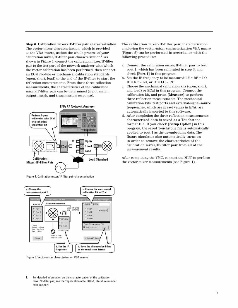
Figure 4. Calibration mixer/IF-filter pair characterization

Figure 5. Vector-mixer characterization VBA macro

1. For detailed information on the characterization of the calibration mixer/IF-filter pair, see the "application note 1408-1, literature number5988-8642EN.

Step 6. Calibration mixer/IF-filter pair characterizationThe vector-mixer characterization, which is provided as the VBA macro, assists the whole process of your calibration mixer/IF-filter pair characterization 1. Asshown in Figure 4, connect the calibration mixer/IF-filterpair to the test port of the network analyzer with whichthe vector calibration has been performed, then connectan ECal module or mechanical calibration standards(open, short, load) to the end of the IF-filter to start thereflection measurements. From these three reflectionmeasurements, the characteristics of the calibrationmixer/IF-filter pair can be determined (input match,output match, and transmission response).

The calibration mixer/IF-filter pair characterizationemploying the vector-mixer characterization VBA macro(Figure 5) can be performed in accordance with thefollowing procedure:

a. Connect the calibration mixer/IF-filter pair to test port 1, which has been calibrated in step 3, and check [Port 1] in this program.

b. Set the IF frequency to be measured: IF = RF + LO, IF = RF – LO, or IF = LO – RF.

c. Choose the mechanical calibration kits (open, short, and load) or ECal in this program. Connect the calibration kit, and press [Measure] to perform three reflection measurements. The mechanical calibration kits, test ports and external-signal-source frequencies, which are preset values in ENA, are automatically imported to this software.

d. After completing the three reflection measurements,characterized data is saved as a Touchstone-format file. If you check [Setup Option] in this program, the saved Touchstone file is automatically applied to port 1 as the de-embedding data. The fixture simulator also automatically turns on in order to remove the characteristics of the calibration mixer/IF-filter pair from all of themeasurement results.

After completing the VMC, connect the MUT to performthe vector-mixer measurements (see Figure 1).

8

3 Scalar-Mixer Calibration (SMC)

The SMC can be used to characterize the conversionloss and reflection parameters of mixers with very highaccuracy, by performing

error correction using a combination of calibrationstandards (ECal or open, short, load) and a power meter.

3.1 Overview of scalar-mixer calibration

For the measurement of the conversion loss in frequency-translating devices, normal full two-port calibration isnot available because of the frequency differencebetween the stimulus and response ports. SMC allowsyou to correct the error terms that reside in a full two-port error model, by using the error model and theexpression based on a new concept 1. The scalar-mixercalibration can correct the following error terms:

• The reflection between the output (stimulus) port of the network analyzer and the input port of the MUT (vector error correction).

• The reflection between the input (response) port of the network analyzer and the output port of the MUT (vector error correction).

• Transmission frequency characteristics in different frequencies (scalar error correction).

In a traditional power-meter calibration, the analyzersource power is calibrated for flatness and linearity over the input frequency range, while the receiver is calibrated for flatness and linearity over the output frequency range. The analyzer is calibrated in the presence of the impedance of the power sensor. In otherwords, the measurements will have optimal accuracy ifthe MUT has the same input match as the power sensor.In this method, the mismatch that exists between theMUT and the network analyzer cannot be corrected.

By using the network analyzer’s one-port calibrationability, the port and MUT input and output reflectioncoefficients can be measured. Using the known vectorreflection coefficients of the test port, the MUT, and the power sensor, SMC corrects for mismatch loss. Since SMC is referenced to a traceable standard (powersensor/ meter measurements), it provides the specifiedmeasurements for conversion loss magnitude.

3.2 Procedure for scalar-mixer calibration

The scalar-mixer calibration procedure is explained byusing the configuration shown in Figure 6. Unlike VMC,SMC does not use the calibration mixer, however the IF-filter is required to select the required IF frequencysuch as RF+LO, RF–LO, or LO–RF.

Figure 6. Configuration of the scalar-mixer calibration

1. For detailed information on the scalar-mixer calibration (SMC) theory, see the application note 1408-1, literature number 5988-8642EN.

9

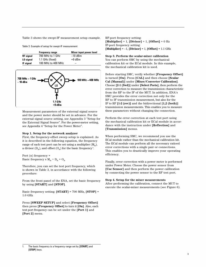
Table 3 shows the swept-IF measurement setup example.

Table 3. Example of setup for swept-IF measurement

Measurement parameters of the external signal sourceand the power meter should be set in advance. For theexternal signal source setting, see Appendix 3 ”Setup forthe External Signal Source”. For the power-meter setting,see Appendix 4 “Setup for the Power Meter”.

Step 1. Setup for the network analyzerFirst, the frequency-offset sweep setup is explained. Asit is described in the following equation, the frequencyrange of each test port can be set using a multiplier (Mn), a divisor (Dn), and offset (On) for the basic frequency 1.

Port (n) frequency = Basic frequency x Mn ÷ Dn + On

Therefore, you can set the test port frequency, which is shown in Table 3, in accordance with the followingprocedure:

From the front panel of the ENA, set the basic frequencyby using [START] and [STOP].

Basic frequency setting: [START] = 700 MHz, [STOP] =1.0 GHz

Press [SWEEP SETUP] and select [Frequency Offset]then press [Frequency Offset] to turn it [On]. Also, eachtest port frequency can be set under the [Port 1] and[Port 2] menu.

RF-port frequency setting: [Multiplier] = 1, [Divisor] = 1, [Offset] = 0 HzIF-port frequency setting: [Multiplier] = –1, [Divisor] = 1, [Offset] = 1.1 GHz

Step 3. Perform the scalar-mixer calibrationYou can perform SMC by using the mechanical calibration kit or the ECal module. In this example, the mechanical calibration kit is used.

Before starting SMC, verify whether [Frequency Offset]is turned [On]. Press [CAL] and then choose [ScalarCal (Manual)] under [Mixer/Converter Calibration].Choose [2-1 (fwd)] under [Select Ports], then perform theerror correction to measure the transmission characteristicfrom the RF to the IF of the MUT. In addition, ENA’sSMC provides the error correction not only for the RF to IF transmission measurement, but also for the IF to RF [1-2 (rev)] and the bidirectional [1,2 (both)]transmission measurements. This enables you to measurethese parameters without changing the connection.

Perform the error correction at each test port using the mechanical calibration kit or ECal module in accor-dance with the instruction under [Reflection] and[Transmission] menus.

When performing SMC, we recommend you use the ECal module rather than the mechanical calibration kit.The ECal module can perform all the necessary ratioederror corrections with a single pair or connections. This enables you to drastically improve your operatingefficiency.

Finally, error correction with a power meter is performedunder Power Meter. Choose the power sensor from [Use Sensor] and then perform the power calibration by connecting the power sensor to the RF test port.

Step 4. Setup for the mixer measurementsAfter performing the calibration, connect the MUT toexecute the scalar-mixer measurements (see Figure 6).

Frequency range Mixer input power level RF signal 700 MHz to 1 GHz –10 dBmLO signal 1.1 GHz (fixed) +9 dBmIF signal 100 MHz to 400 MHz –

1. The basic frequency is a frequency range set by [START] and [STOP] keys.

10

4 Mixer Measurements

There are several measurement parameters involvedwith mixer measurements, such as conversion loss,return loss, conversion compression, isolation, and intermodulation

distortion. This section describes several proceduresand hardware setups for measuring these parameters.

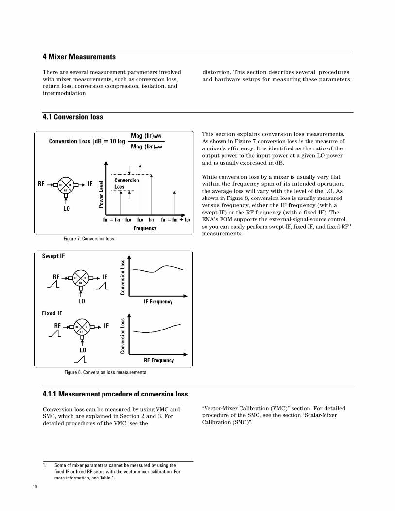
4.1 Conversion loss

This section explains conversion loss measurements. As shown in Figure 7, conversion loss is the measure of a mixer’s efficiency. It is identified as the ratio of theoutput power to the input power at a given LO powerand is usually expressed in dB.

While conversion loss by a mixer is usually very flatwithin the frequency span of its intended operation,the average loss will vary with the level of the LO. Asshown in Figure 8, conversion loss is usually measuredversus frequency, either the IF frequency (with aswept-IF) or the RF frequency (with a fixed-IF). TheENA’s FOM supports the external-signal-source control,so you can easily perform swept-IF, fixed-IF, and fixed-RF 1

measurements.

4.1.1 Measurement procedure of conversion loss

Conversion loss can be measured by using VMC andSMC, which are explained in Section 2 and 3. Fordetailed procedures of the VMC, see the

“Vector-Mixer Calibration (VMC)” section. For detailedprocedure of the SMC, see the section “Scalar-MixerCalibration (SMC)”.

Figure 8. Conversion loss measurements

Figure 7. Conversion loss

1. Some of mixer parameters cannot be measured by using the fixed-IF or fixed-RF setup with the vector-mixer calibration. For more information, see Table 1.

11

4.1.2 Example of conversion loss measurements(VMC/SMC)

Figure 9 shows an example of conversion loss measure-ments made with VMC and SMC. These measurementscan be performed with the operations that are explainedin sections 2 and 3. As shown in this figure, both datacorrelate well; hence you can perform highly accurateconversion loss measurements using either the VMC orthe SMC technique.

VMC allows you to measure phase and absolute groupdelay of conversion loss, which traditionally has been avery difficult and noisy measurement. Figure 10 showsthe measurement results of magnitude, phase, andgroup delay of conversion loss.

Figure 11 shows the conversion loss measurement data comparison made with SMC versus a traditionalpower-meter calibration. This figure clearly reveals thata simple power-meter calibration cannot remove errorterms such as source match, load match, and directivity;therefore, the measurement trace has ripple due to theeffects of these error terms.

Figure 9. Comparison of conversion loss measurement results (VMC vs. SMC)

Figure 10. Conversion loss measurement example with VMC

Figure 11. Conversion loss measurement comparison (SMC vs. Power Cal.)

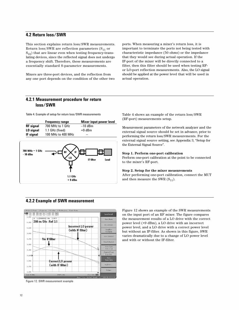
Figure 12. SWR measurement example

12

4.2.1 Measurement procedure for return loss/SWR

Table 4. Example of setup for return loss/SWR measurements Table 4 shows an example of the return loss/SWR (RF-port) measurements setup.

Measurement parameters of the network analyzer and theexternal signal source should be set in advance, prior toperforming the return loss/SWR measurements. For theexternal signal source setting, see Appendix 3, “Setup forthe External Signal Source”.

Step 1. Perform one-port calibrationPerform one-port calibration at the point to be connectedto the mixer’s RF-port.

Step 2. Setup for the mixer measurementsAfter performing one-port calibration, connect the MUTand then measure the SWR (S11).

4.2 Return loss/SWR

This section explains return loss/SWR measurements.Return loss/SWR are reflection parameters (S11 orS22) that are linear even when testing frequency-trans-lating devices, since the reflected signal does not undergoa frequency shift. Therefore, these measurements areessentially standard S-parameter measurements.

Mixers are three-port devices, and the reflection fromany one port depends on the condition of the other two

ports. When measuring a mixer’s return loss, it is important to terminate the ports not being tested withcharacteristic impedance (50 ohms) or the impedancethat they would see during actual operation. If the IF-port of the mixer will be directly connected to a filter, then this filter should be used when testing RF- or LO-port reflection measurements. Also, the LO signalshould be applied at the power level that will be used inactual operation.

Frequency range Mixer input power levelRF signal 700 MHz to 1 GHz –10 dBmLO signal 1.1 GHz (fixed) +9 dBmIF signal 100 MHz to 400 MHz –

4.2.2 Example of SWR measurement

Figure 12 shows an example of the SWR measurementson the input port of an RF mixer. The figure comparesthe measurement results of a LO drive with the correctpower level (+9 dBm), a LO drive with an incorrectpower level, and a LO drive with a correct power levelbut without an IF-filter. As shown in this figure, SWRvaries dramatically due to a change of LO power leveland with or without the IF-filter.

13

4.3 Conversion compression

This section explains the conversion compression measurements. Conversion compression is a measure ofthe maximum RF input signal level for which the mixerwill provide linear operation (Figure 13). Conversionloss is the ratio of the IF output level to the RF inputlevel, and this value remains constant over a specifiedinput power range. When the input power level exceedsa certain maximum, the constant ratio between IF andRF power levels will begin to change. The point at which the ratio has decreased by 1 dB is called the 1-dB compression point.

4.3.1 Measurement procedure for conversion compression

The conversion compression can be measured by usingthe power sweep function on the ENA.

Table 5 shows an example of conversion compressionmeasurements setup.

Table 5. Example of setup for conversion compression measurements

Measurement parameters of the network analyzer, theexternal signal source, and the power meter should be set in advance, prior to performing the conversioncompression measurement. For the external signal sourcesetting, see Appendix 3, “Setup for the External SignalSource”. For the power meter setting, see Appendix 4,“Setup for the Power Meter”.

Step 1. Setup for the network analyzerThe setup procedure of power sweep is explained as follows: From the front panel of the ENA, set the carrier-wave(CW) frequency by using [SWEEP SETUP] and set [CWFreq] (700 MHz) under [Power]. Then, press [SweepType] under [SWEEP SETUP] and choose [PowerSweep]. Set the power range (–20 dBm to +5 dBm) byusing [START] and [STOP].

As shown in Table 5, RF and IF frequencies are different soeach test port frequency needs to be set independentlywith the frequency-offset function. For the frequency-offset sweep setting, see the “Procedure for scalar-mixercalibration” section.

Figure 13. Conversion compression

Frequency range Mixer input power levelRF signal 700 MHz (fixed) –20 dBm to +5 dBmLO signal 1.1 GHz (fixed) +9 dBmIF signal 400 MHz (fixed) –

14

Step 2. Perform the SMCSMC should be performed before measurements. For the SMC procedure, see “Procedure for scalar-mixer calibration”.

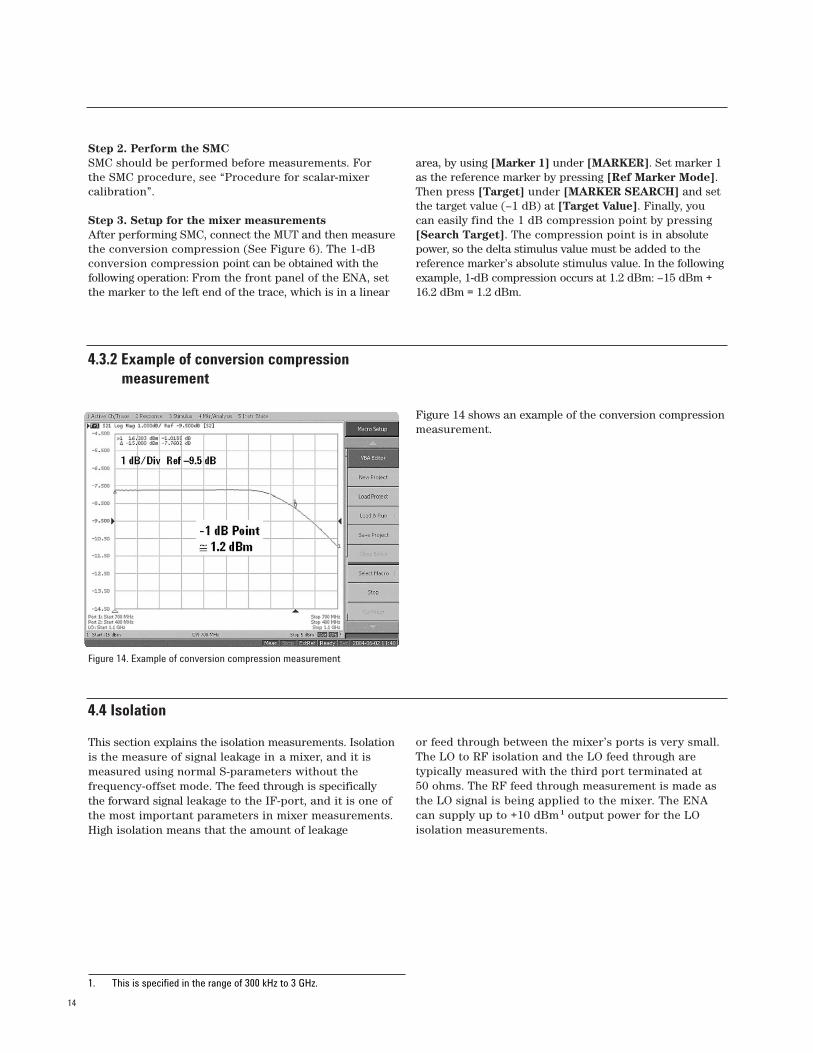
Step 3. Setup for the mixer measurementsAfter performing SMC, connect the MUT and then measurethe conversion compression (See Figure 6). The 1-dBconversion compression point can be obtained with the following operation: From the front panel of the ENA, setthe marker to the left end of the trace, which is in a linear

area, by using [Marker 1] under [MARKER]. Set marker 1as the reference marker by pressing [Ref Marker Mode].Then press [Target] under [MARKER SEARCH] and setthe target value (–1 dB) at [Target Value]. Finally, youcan easily find the 1 dB compression point by pressing[Search Target]. The compression point is in absolutepower, so the delta stimulus value must be added to the reference marker’s absolute stimulus value. In the followingexample, 1-dB compression occurs at 1.2 dBm: –15 dBm +16.2 dBm = 1.2 dBm.

4.3.2 Example of conversion compressionmeasurement

Figure 14 shows an example of the conversion compressionmeasurement.

4.4 Isolation

This section explains the isolation measurements. Isolationis the measure of signal leakage in a mixer, and it ismeasured using normal S-parameters without the frequency-offset mode. The feed through is specifically the forward signal leakage to the IF-port, and it is one ofthe most important parameters in mixer measurements.High isolation means that the amount of leakage

or feed through between the mixer’s ports is very small.The LO to RF isolation and the LO feed through are typically measured with the third port terminated at 50 ohms. The RF feed through measurement is made asthe LO signal is being applied to the mixer. The ENAcan supply up to +10 dBm 1 output power for the LO isolation measurements.

Figure 14. Example of conversion compression measurement

1. This is specified in the range of 300 kHz to 3 GHz.

15

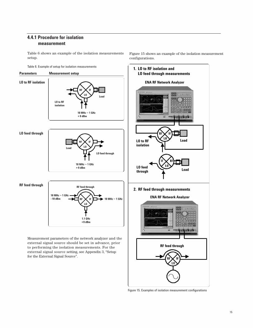
4.4.1 Procedure for isolation measurement

Table 6 shows an example of the isolation measurementssetup.

Table 6. Example of setup for isolation measurements

Measurement parameters of the network analyzer and theexternal signal source should be set in advance, priorto performing the isolation measurements. For theexternal signal source setting, see Appendix 3, “Setup for the External Signal Source”.

Figure 15 shows an example of the isolation measurementconfigurations.

Parameters Measurement setup

LO to RF isolation

LO feed through

RF feed through

Figure 15. Examples of isolation measurement configurations

10 MHz ~ 1 GHz+ 9 dBm

LO to RF isolation

Load

RF IF

LO

Load

10 MHz ~ 1 GHz+ 9 dBm

LO feed through

RF IF

LO

10 MHz ~ 1 GHz–10 dBm 10 MHz ~ 1 GHz

1.1 GHz+9 dBm

RF feed through

RF IF

LO

1. LO to RF isolation and LO feed through measurements

2. RF feed through measurements

ENA RF Network Analyzer

LO to RFisolation

Load

LoadLO feedthrough

ENA RF Network Analyzer

RF feed through

16

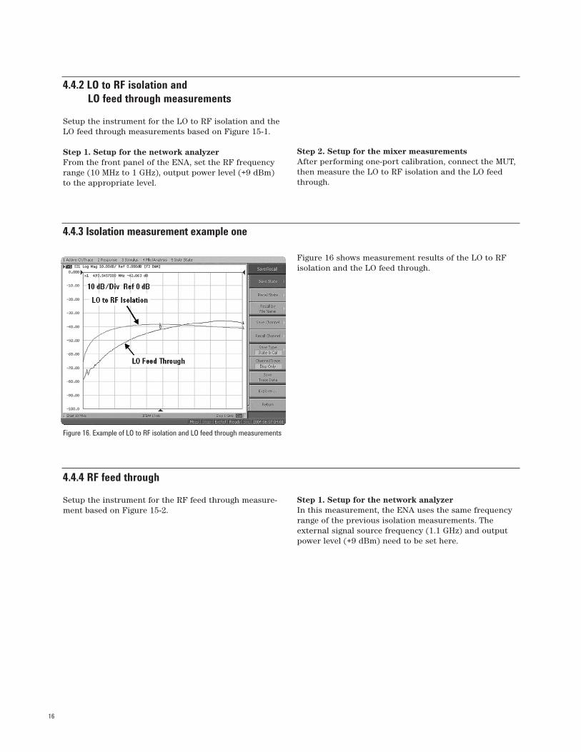
4.4.2 LO to RF isolation and LO feed through measurements

Setup the instrument for the LO to RF isolation and theLO feed through measurements based on Figure 15-1.

Step 1. Setup for the network analyzerFrom the front panel of the ENA, set the RF frequencyrange (10 MHz to 1 GHz), output power level (+9 dBm)to the appropriate level.

Step 2. Setup for the mixer measurementsAfter performing one-port calibration, connect the MUT,then measure the LO to RF isolation and the LO feedthrough.

4.4.3 Isolation measurement example one

Figure 16 shows measurement results of the LO to RFisolation and the LO feed through.

4.4.4 RF feed through

Setup the instrument for the RF feed through measure-ment based on Figure 15-2.

Step 1. Setup for the network analyzerIn this measurement, the ENA uses the same frequencyrange of the previous isolation measurements. The external signal source frequency (1.1 GHz) and outputpower level (+9 dBm) need to be set here.

Figure 16. Example of LO to RF isolation and LO feed through measurements

17

4.4.5 Isolation measurement example two

Figure 17 shows the measurement result of the RF feedthrough.

4.5 Two-tone third-order intermodulationdistortion

This section explains the two-tone third-order intermodula-tion distortion measurements. Intermodulation distortionis a common problem in narrowband systems. It is theunwanted frequency components resulting from theinteraction of two (f1 and f2) or more spectral compo-nents passing through a device with non-linear behaviorsuch as a mixer. The unwanted components are relatedto the fundamental components by sums and differences of the fundamentals and various harmonics: nf1 ± mf2.

|n| + |m| is called the order of intermodulation products,so 2f1 – f2 and 2f2 – f1 are called third-order intermodula-tion products.

In this measurement, two closely spaced fixed frequenciesof equal amplitude are input at the mixer’s RF-port,while a single frequency is used to drive the mixer’s LO port.

4.5.1 Procedure for intermodulation distortion measurement

Table 7. Example of setup for intermodulation distortion measurement Table 7 shows an example of intermodulation distortionmeasurement setup.

Figure 17. Example of RF feed through measurement

Frequency range Mixer input power levelRF1 signal 1 GHz (fixed) –10 dBmRF2 signal 1.00003 GHz (fixed) –10 dBmLO signal 900 MHz (fixed) +9 dBmIF1 signal 100 MHz –IF2 signal 100.03 MHz –

IF = 100 MHzIF = 100 MHz

3rd order intermodulation productsIM31 = 2RF1 – RF2 – LOIM32 = 2RF2 – RF1 – LO

900 MHz+ 9 dBm

RF1 1 GHz, –10 dBmRF2 1.00003 GHz, –10 dBm RF IF

LO

18

The third-order intermodulation products can be calculatedwith the following equations:

IM3 1 = 2RF1 – RF2 – LO = 99.97 MHzIM3 2 = 2RF2 – RF1 – LO = 100.06 MHz

Measurement parameters of the network analyzer andthe external signal source should be set in advance,prior to performing an intermodulation distortion measurement. For the external signal source setting, see Appendix 3 “Setup for the External Signal Source”.

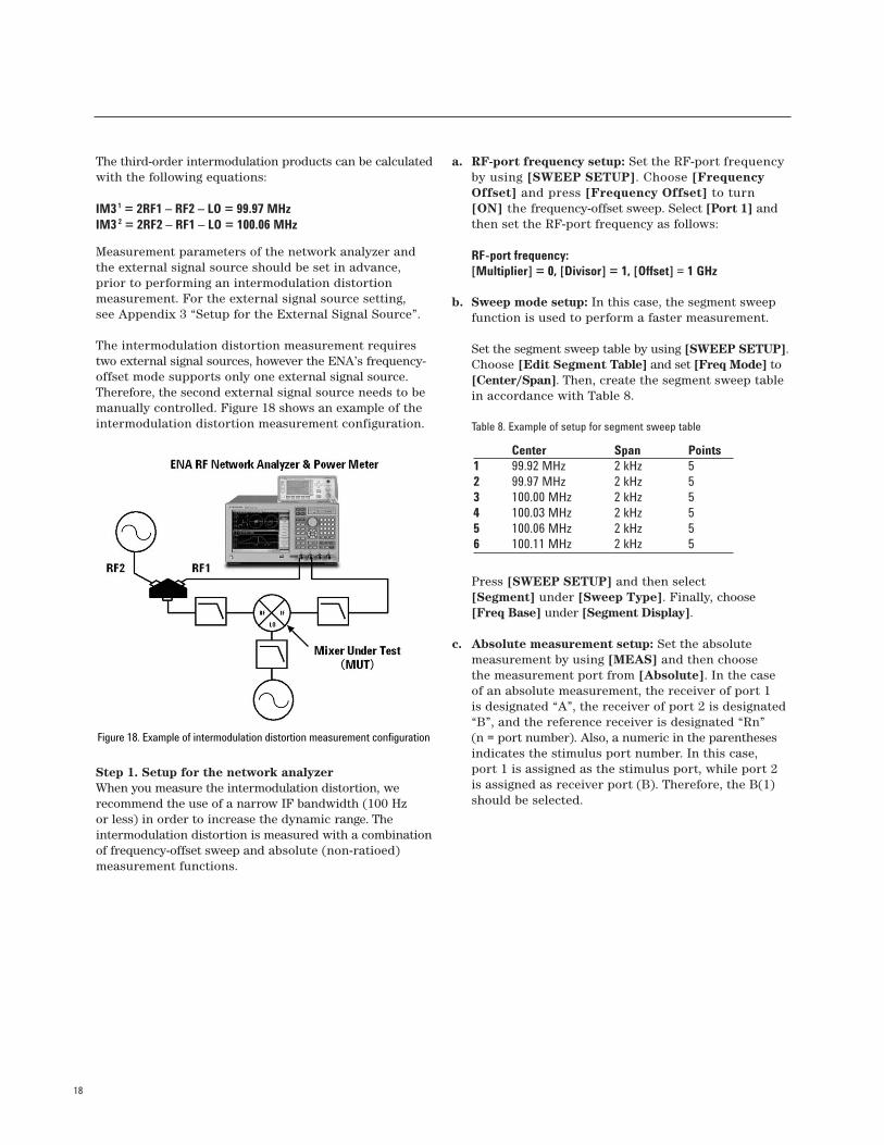
The intermodulation distortion measurement requirestwo external signal sources, however the ENA’s frequency-offset mode supports only one external signal source.Therefore, the second external signal source needs to bemanually controlled. Figure 18 shows an example of theintermodulation distortion measurement configuration.

Step 1. Setup for the network analyzerWhen you measure the intermodulation distortion, we recommend the use of a narrow IF bandwidth (100 Hz or less) in order to increase the dynamic range. The intermodulation distortion is measured with a combinationof frequency-offset sweep and absolute (non-ratioed)measurement functions.

a. RF-port frequency setup: Set the RF-port frequency by using [SWEEP SETUP]. Choose [Frequency Offset] and press [Frequency Offset] to turn [ON] the frequency-offset sweep. Select [Port 1] andthen set the RF-port frequency as follows:

RF-port frequency: [Multiplier] = 0, [Divisor] = 1, [Offset] = 1 GHz

b. Sweep mode setup: In this case, the segment sweep function is used to perform a faster measurement.

Set the segment sweep table by using [SWEEP SETUP].Choose [Edit Segment Table] and set [Freq Mode] to [Center/Span]. Then, create the segment sweep table in accordance with Table 8.

Table 8. Example of setup for segment sweep table

Press [SWEEP SETUP] and then select [Segment] under [Sweep Type]. Finally, choose [Freq Base] under [Segment Display].

c. Absolute measurement setup: Set the absolute measurement by using [MEAS] and then choose the measurement port from [Absolute]. In the case of an absolute measurement, the receiver of port 1 is designated “A”, the receiver of port 2 is designated“B”, and the reference receiver is designated “Rn” (n = port number). Also, a numeric in the parenthesesindicates the stimulus port number. In this case, port 1 is assigned as the stimulus port, while port 2 is assigned as receiver port (B). Therefore, the B(1) should be selected.

Center Span Points1 99.92 MHz 2 kHz 52 99.97 MHz 2 kHz 53 100.00 MHz 2 kHz 54 100.03 MHz 2 kHz 55 100.06 MHz 2 kHz 56 100.11 MHz 2 kHz 5

Figure 18. Example of intermodulation distortion measurement configuration

19

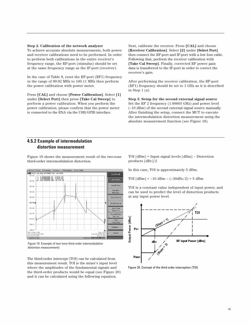
Figure 19. Example of two-tone third-order intermodulationdistortion measurement)

Step 2. Calibration of the network analyzerTo achieve accurate absolute measurements, both powerand receiver calibrations need to be performed. In orderto perform both calibrations in the entire receiver’s frequency range, the RF-port (stimulus) should be set at the same frequency range as the IF-port (receiver).

In the case of Table 8, reset the RF-port (RF1) frequencyin the range of 99.92 MHz to 100.11 MHz then performthe power calibration with power meter.

Press [CAL] and choose [Power Calibration]. Select [1]under [Select Port] then press [Take Cal Sweep] toperform a power calibration. When you perform thepower calibration, please confirm that the power meteris connected to the ENA via the USB/GPIB interface.

Next, calibrate the receiver. Press [CAL] and choose[Receiver Calibration]. Select [2] under [Select Port]then connect the RF-port and IF-port with a low loss cable.Following that, perform the receiver calibration with[Take Cal Sweep]. Finally, corrected RF power gain data is transferred to the IF-port in order to correct thereceiver’s gain.

After performing the receiver calibration, the RF-port(RF1) frequency should be set to 1 GHz as it is describedin Step 1 (a).

Step 3. Setup for the second external signal sourceSet the RF 2 frequency (1.00003 GHz) and power level(–10 dBm) of the second external signal source manually.After finishing the setup, connect the MUT to executethe intermodulation distortion measurement using theabsolute measurement function (see Figure 18).

4.5.2 Example of intermodulation distortion measurement

Figure 19 shows the measurement result of the two-tonethird-order intermodulation distortion.

The third-order intercept (TOI) can be calculated from this measurement result. TOI is the mixer’s input levelwhere the amplitudes of the fundamental signals andthe third-order products would be equal (see Figure 20)and it can be calculated using the following equation.

TOI [dBm] = Input signal levels [dBm] – Distortion products [dBc]/2

In this case, TOI is approximately 5 dBm.

TOI [dBm] = –10 dBm – (–30dBc/2) = 5 dBm

TOI is a constant value independent of input power, andcan be used to predict the level of distortion products at any input power level.

Figure 20. Concept of the third-order interception (TOI)

20

Summary

There are many challenges associated with makingmeasurements on non-linear frequency-translatingdevices such as mixers. It is difficult to accurately evaluatemixers due to complex measurement configurations and to account for unwanted error signals.

The FOM on the ENA RF network analyzers providesvarious kinds of functions that can solve these typicalissues. In particular,

advanced mixer-calibration functions such as VMC and SMC permit highly accurate mixer measurements.In addition, the absolute measurement function with the power and the receiver calibration enables you toperform accurate intermodulation distortion measure-ments. Hence, the ENA’s FOM makes all required mixer measurements fast and easy, while giving you more confidence in the measurement results.

Appendix 1: Calibration Mixer Attributes andConsiderations

Frequency range: The frequency range of a calibrationmixer should be the same or wider than the frequencyrange of the MUT. If you want to test multiple MUTswith a single calibration mixer, this calibration mixershould cover the frequency range of all the MUTs tobe tested.

Return loss: VMC corrects for the mismatch errors associated with the reflected signal of the fundamentalfrequency. However, the harmonic and spurious productscan reflect off the mixer and network analyzer test portsand create error terms. Therefore a device with betterreturn loss will yield lower uncertainty. If RF- and IF-filtering are used before and after the mixer respectively,the effects of poor return loss can be reduced, and if theconversion loss of the mixer is low enough, attenuatorscan be used to improve mismatch errors.

Conversion loss: To obtain accurate calibration results,the one-way conversion loss of the calibration mixer/IF-filter pair should be less than 10 dB. If the one-wayconversion loss of the calibration mixer exceeds 15 dB,the accuracy of the calibration is severely degraded.

Conversion loss reciprocity: The main requirement of a calibration mixer is that it should be reciprocal.Reciprocity means that the forward and reverse conver-sion loss magnitude and phase are equal. Forward conversion loss is defined as the loss that occurs whenan RF signal is incident upon port 1 and an IF signal is measured at port 2. On the other hand, reverse conversion loss is defined as the loss that happens when an IF signal is incident upon port 2 and an RF signal is measured at port 1. The reason for the reciprocity requirement is that the calibration processcalculates the net response of the forward and reversemixer conversion loss by measuring the portion of thesignal that travels through the filter and reflects off the calibration standards. In calculating the error terms,the assumption is made that the forward and reverseconversion losses are the same, and from here, the one-way characteristic of the calibration mixer is determined 1.

1. For detailed information on the vector-mixer calibration (VMC) theory and frequency-offset error models, see application note 1408-1, literature number 5988-8642EN.

21

High-order mixing products (spurious products): The spurious generation of a calibration mixer should be low,as spuriousness can result in measurement errors. TheFOM includes the avoid spurious function, which canreduce the effects of various spurs during the calibrationand measurement process (see Figure 21). Another practical technique is to slightly change the stimulus orresponse frequencies or number of points to avoid spurs.

Isolation: There are six mixer isolation terms; RF to IFand LO, LO to RF and IF, IF to RF and LO. The LO leakageterm can be a significant error causing a spuriousresponse, due to the high power levels of the LO. Thus, it is critical to reduce the amount of LO leakage in orderto achieve an accurate VMC. A good calibration mixerhas at least 20 dB of LO to RF and LO to IF isolation.The LO leakage problem is that the LO signal leakingthrough the RF or IF port can reflect off the network analyzer port and re-enter the mixer and mix with theother products to create a mismatch error signal. It alsocan leak to the reference channel path and createadditional errors.

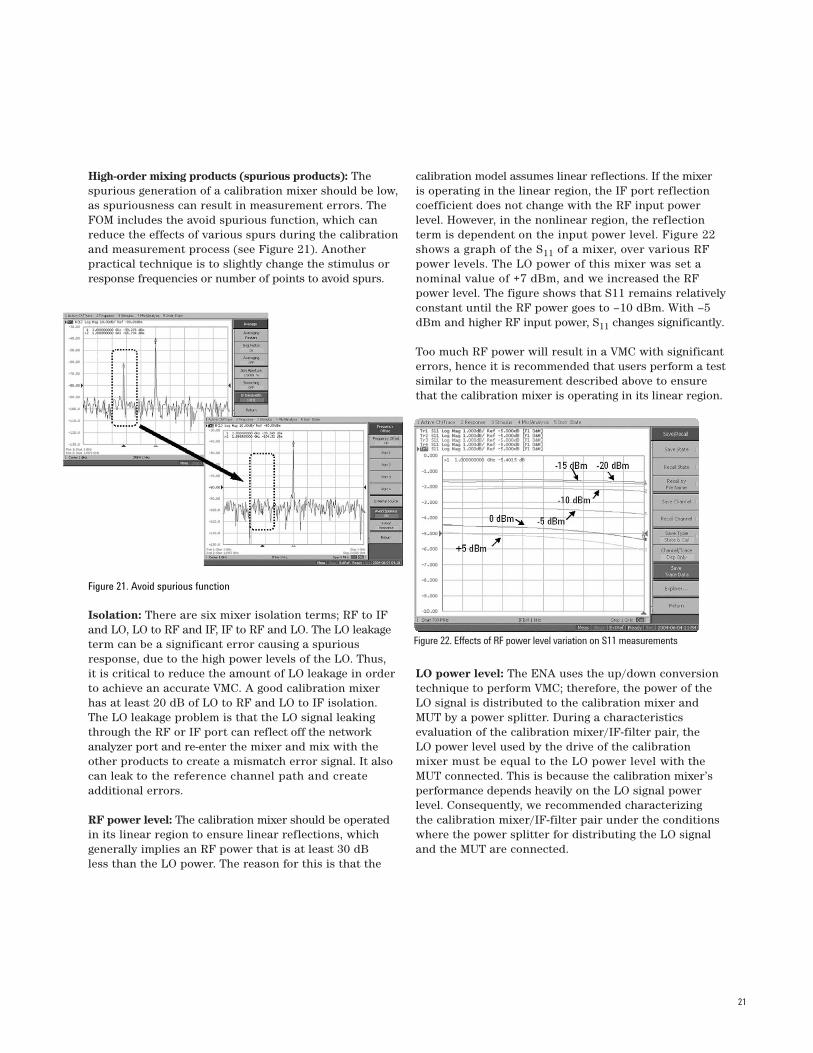
RF power level: The calibration mixer should be operatedin its linear region to ensure linear reflections, whichgenerally implies an RF power that is at least 30 dB less than the LO power. The reason for this is that the

calibration model assumes linear reflections. If the mixeris operating in the linear region, the IF port reflectioncoefficient does not change with the RF input powerlevel. However, in the nonlinear region, the reflectionterm is dependent on the input power level. Figure 22shows a graph of the S11 of a mixer, over various RFpower levels. The LO power of this mixer was set anominal value of +7 dBm, and we increased the RFpower level. The figure shows that S11 remains relativelyconstant until the RF power goes to –10 dBm. With –5dBm and higher RF input power, S11 changes significantly.

Too much RF power will result in a VMC with significanterrors, hence it is recommended that users perform a testsimilar to the measurement described above to ensurethat the calibration mixer is operating in its linear region.

LO power level: The ENA uses the up/down conversiontechnique to perform VMC; therefore, the power of theLO signal is distributed to the calibration mixer andMUT by a power splitter. During a characteristics evaluation of the calibration mixer/IF-filter pair, the LO power level used by the drive of the calibrationmixer must be equal to the LO power level with theMUT connected. This is because the calibration mixer’sperformance depends heavily on the LO signal powerlevel. Consequently, we recommended characterizing the calibration mixer/IF-filter pair under the conditionswhere the power splitter for distributing the LO signaland the MUT are connected.

Figure 22. Effects of RF power level variation on S11 measurements

Figure 21. Avoid spurious function

a. Launch the balancedmixer characterizationmenu

b. Characterizedmixer data filesare automaticallyloaded

c. Choose the measurement port

d. Execute themeasurement

22

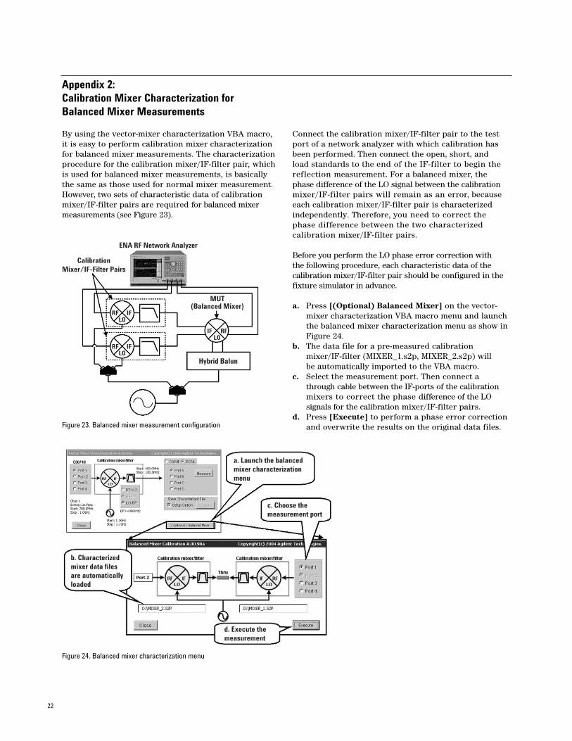
Appendix 2: Calibration Mixer Characterization for Balanced Mixer Measurements

By using the vector-mixer characterization VBA macro,it is easy to perform calibration mixer characterizationfor balanced mixer measurements. The characterizationprocedure for the calibration mixer/IF-filter pair, whichis used for balanced mixer measurements, is basicallythe same as those used for normal mixer measurement.However, two sets of characteristic data of calibrationmixer/IF-filter pairs are required for balanced mixermeasurements (see Figure 23).

Connect the calibration mixer/IF-filter pair to the testport of a network analyzer with which calibration hasbeen performed. Then connect the open, short, and load standards to the end of the IF-filter to begin thereflection measurement. For a balanced mixer, thephase difference of the LO signal between the calibrationmixer/IF-filter pairs will remain as an error, becauseeach calibration mixer/IF-filter pair is characterizedindependently. Therefore, you need to correct thephase difference between the two characterized calibration mixer/IF-filter pairs.

Before you perform the LO phase error correction with the following procedure, each characteristic data of the calibration mixer/IF-filter pair should be configured in thefixture simulator in advance.

a. Press [(Optional) Balanced Mixer] on the vector-mixer characterization VBA macro menu and launch the balanced mixer characterization menu as show in Figure 24.

b. The data file for a pre-measured calibration mixer/IF-filter (MIXER_1.s2p, MIXER_2.s2p) will be automatically imported to the VBA macro.

c. Select the measurement port. Then connect a through cable between the IF-ports of the calibration mixers to correct the phase difference of the LO signals for the calibration mixer/IF-filter pairs.

d. Press [Execute] to perform a phase error correction and overwrite the results on the original data files.

Figure 24. Balanced mixer characterization menu

ENA RF Network Analyzer

CalibrationMixer/IF-Filter Pairs

MUT(Balanced Mixer)

Hybrid Balun

RF IFLO

RFIFLO

RF IFLO

Figure 23. Balanced mixer measurement configuration

23

Appendix 3: Setup for the External Signal Source

The ENA allows you to control the external signal sourceconnected to the USB/GPIB interface 1. Typical Agilentsignal sources such as ESG, PSG, and the 86xx Series are supported by the ENA as the standard.

To use an external signal source, we recommend that theexternal signal source's internal-reference signal output connector (Ref. Out) and the ENA's external-referencesignal input connector (Ref. In) should be connected to each other with a BNC cable. This ensures a stablemeasurement because the ENA is phase-locked to theexternal signal source's frequency reference signal.

From the front panel of the ENA, set the GPIB addressof the external signal source by using the [SYSTEM].Press the [Misc Setup] and choose [GPIB Setup] andthen enter the external signal source address at [SignalGenerator Address]. Additionally, the desired signalsource can be selected under this menu.

Next, set the power level and frequency range of theexternal signal source. In the case of VMC, the outputpower of the external signal source is distributed to the calibration mixer and MUT by a power splitter.Consequently, the power level needs to be set in consideration of the power splitter’s loss (about 6 dB).

From the front panel of the ENA, set the power level byusing [SWEEP SETUP].

Press [Frequency Offset] and choose [Power] under[External Source] and then set the power level.

As described in the following equation, the externalsource frequency range can be set using a multiplier(MLO), a divisor (DLO), and offset (OLO) for the basic frequency 2.

External signal source frequency (LO) = Basic Frequency xMLO ÷ DLO + OLO

For example, 1.1 GHz fixed LO frequency can be setusing the following values.

External signal source (LO) setting: [Multiplier] = 0,[Divisor] = 1, [Offset] = 1.1 GHz

The external signal source frequency can also be setwith [Start] and [Stop], although the setting mentionedabove is recommended. This allows you to automaticallyretain the offset value even if you have changed the setting range of the basic frequency, since the externalsignal source frequency is defined as a formula.

Finally, the control of an external signal source isexplained. The LO frequency (LO) setting can be displayed under the screen of the ENA by using [LOFrequency] to turn it [On]. Then press [Control] toturn the external signal source control [On], whichallows you to send parameters such as frequency rangeand power level to the external signal source and start the control.

Appendix 4: Setup for the Power Meter

The ENA allows you to control the power meter connectedto the USB/GPIB interface. From the front panel of theENA, set the GPIB address of the power meter by using[SYSTEM]. Press [Misc Setup] and choose [GPIB Setup]and then enter the power meter address at [PowerMeter Address].

1. A USB/GPIB interface is necessary to control ENA peripherals, suchas power meters or source generators for mixer measurements. Agilent’s 82357A USB/GPIB interface is recommended.

2. The basic frequency is a frequency range set by [START] and [STOP] keys.

Related Literature

These documents are available from the library onAgilent’s website: www.agilent.com

1. Mixer Transmission Measurements Using The Frequency Converter Application, application note 1408-1, literature number 5988-8642EN

2. Mixer Conversion-Loss and Group Delay Measurement Techniques and Comparisons,application note 1408-2, literature number 5988-9619EN

3. Improving Measurement and Calibration Accuracy using the Frequency Converter Application,application note 1408-3, iterature number 5988-9642EN

4. Novel Method for Vector Mixer Characterization and Mixer Test System Vector Error Correction,white paper, literature number 5988-7826EN

5. Comparison of Mixer Characterization using New Vector Characterization Techniques,white paper, literature number 5988-7827EN

6. Improving Network Analyzer Measurements of Frequency-translating Devices,application note 1287-7, literature number 5966-3318E

Web ResourcesFor additional information on the ENA visit:www.agilent.com/find/ena

www.agilent.com/find/emailupdatesGet the latest information on the products and applications you select.

www.agilent.com/find/agilentdirectQuickly choose and use your test equipment solutions with confidence.

www.agilent.com/find/openAgilent Open simplifies the process of connecting and programming test systems to help engineers design, validate and manufacture electronic products. Agilent offers open connectivity for a broad range of system-ready instruments, open industry software, PC-standard I/O and global support,which are combined to more easily integrate test system development.

Agilent Email Updates

Agilent Direct

AgilentOpen

www.agilent.com

For more information on Agilent Technologies’ products, applicationsor services, please contact your local Agilent office. The complete listis available at:

www.agilent.com/find/contactus

Product specifications and descriptions in this document subjectto change without notice.

© Agilent Technologies, Inc. 2004, 2005, 2007Printed in USA, May 7, 20075989-1420EN

Remove all doubt

Our repair and calibration services will get your equipmentback to you, performing like new, when promised. You will get full value out of your Agilent equipment throughout its lifetime. Your equipment will be serviced by Agilent-trainedtechnicians using the latest factory calibration procedures,automated repair diagnostics and genuine parts. You willalways have the utmost confidence in your measurements.

Agilent offers a wide range of additional expert test and measurement services for your equipment, including initialstart-up assistance onsite education and training, as well asdesign, system integration, and project management.

For more information on repair and calibration services, go to:

www.agilent.com/find/removealldoubt