DEPARTMENT OF AGRICULTURAL AND RESOURCE ECONOMICSDIVISION OF AGRICULTURE AND NATURAL RESOURCES

UNIVERSITY OF CALIFORNIA AT BERKELEY

WORKING PAPER NO. 617

AGRICULTURAL POLICIES AND MIGRATIONIN A U.S.-MEXICO FREE TRADE AREA:

A COMPUTABLE GENERAL EQUILIBRIUM ANALYSIS

by

Sherman RobinsonUniversity of California, Berkeley

Mary E. BurfisherEconomic Resear61. Service

U.S. Department of Agriculture

Raul Hinojosa-Ojeda .University of California, Los Angeles

Karen E. ThierfelderEconomic Research Service

U.S. Department of Agriculture

WAITE MEMORIAL BOOK COLLECTIONDEPT. OF AG. AND APPLIED ECONOMICS

1994 BUFORD AVE. 232 COBUNIVERSITY OF MINNESOTAST. PAUL, MN 55108 U.S.A.

California Agricultural Experiment StationGiannini Foundation of Agricultural Economics

December 1991

7

•..

3 nv3v 55

7Table of Contents

1. Introduction

2. Core Three—Country CGE Model 3

3. Import Demand Equations 9

4. Migration

5. Agricultural Programs

12

135.1 Mexican Agricultural Programs 165.2 U.S. Agricultural Programs 20

6. Model Results 226.1 Scenarios 226.2 Aggregate results 246.3 Migration and Farm Program Expenditure 29

7. Conclusion 32

Appendix: The US-Mexico FTA—CGE Model •37

Abstract

CA U.S.—Mexico agreement to form a free trade area (FTA) is analyzed using an 11-sector,three-country, computable general equilibrium (CGE) model that explicitly models farmprograms and labor migration. The model also uses a flexible functional form for specifyingsectoral import demand functions, which is an empirical improvement over earlierspecifications using a constant elasticity of substitution (CES) function. The model identifiesthe trade-offs among bilateral trade growth, labor migration, and agricultural programexpenditures under alternative FTA scenarios. Trade liberalization in agriculture greatlyincreases rural-urban migration within Mexico and migration from Mexico to the U.S.Migration is reduced if Mexico grows relative to the U.S. and also if Mexico retains farmsupport programs. However, the more support that is provided to the Mexican agriculturalsector, the smaller is bilateral trade growth.

1. Introduction

In June 1990, Mexican President Salinas de Gortari and President Bush agreed to

negotiate the establishment of a free trade area (FTA) between their two countries. An

agreement between the U.S. and Mexico will complement the U.S.-Canada free trade

agreement, which went into effect in January 1988, creating a North American free trade

area (or NAFTA). The trade block will not, in fact, be a "free trade" area, in which all trade

barriers among member countries are removed. Assuming that U.S.-Mexico negotiations

follow the precedent set in the U.S.-Canada agreement, tariffs will fall to zero over intervals

negotiated sector by sector, but liberalization of nontariff barriers . will be selective.

U.S.-Canadian agricultural trade, although substantially liberalized by the gradual

elimination of tariffs, was liberalized less than other sectors. Domestic agricultural programs

in both countries, and the nontariff barriers used to support them, remained essentially intact

(Goodloe and Link (1991)1.

Drawing on experience with the U.S.-Canada FTA, realistic analysis of a U.S.-Mexico

FTA should consider alternative treatments of agricultural trade, including partial

liberalization scenarios and scenarios for retention or restructuring of domestic agricultural

programs. This article provides an analysis of the U.S.-Mexico free trade agreement using

a three-country, 11-sector, computable general equilibrium (CGE) model. Our "FTA-CGE"

model focuses on three modeling issues which are especially important in analyzing a

U.S.-Mexico FTA. First is the explicit modeling of agricultural policies in the two countries

in order to capture the linkages, particularly in Mexico, between bilateral agricultural trade

bathers and social policy objectives. Mexican agricultural policies that are modeled include

1

tariffs; import quotas for beans, corn,and other grains; input subsidies to producers and

processors; and low income tortilla subsidies to consumers. The tariff equivalents of quotas

are determined endogenously and are not treated as fixed ad valorem wedges. U.S. policies

included in the model are deficiency payments and the Export Enhancement Program (EEP).

Since government agricultural program expenditures on subsidies for farmers and processors

are included in the model, one can analyze the fiscal impacts of changes in agricultural

output and trade.

A second issue is labor migration, and the effect that liberalization of trade in

agriculture in particular is likely to have in stimulating rural-urban migration in Mexico and

migration from Mexico to the U.S. rural and urban labor markets. Migration issues are not

explicitly part of the FTA negotiations. However, labor migration is sensitive to relative

economic conditions in the two countries, and to the mix of trade and domestic policies in

Mexican agriculture. The FTA-CGE model includes migration equations and the results

indicate the importance of migration in different FTA scenarios.

The third modeling issue concerns the specification of import demand. The standard

approach in trade-focused CGE models has been to adopt the Armington assumption of

product differentiation coupled with use of a constant elasticity of substitution (CES) import

aggregation function. The CES specification has been criticized because it constrains import

demand equations to have an expenditure elasticity of one, and also implies that every

country has market power in its export markets.' Brown (1987) shows that these

assumptions have led earlier multi-country trade models to generate unrealistically large

terms-of-trade effects under trade-liberalization scenarios. The FTA-CGE model employs the

Almost Ideal Demand System (AIDS) to describe import demand, a flexible functional form

•'The CES formulation has also been criticized on econometric grounds [Alston et al. (1990)].

2

which allows non-unitary expenditure elasticities and yields more realistic empirical results,

while retaining the essential property of imperfect substitutability.

In sections 2 to 5, we present the core CGE model and describe how we model import

demand, migration, and agricultural programs. In section 6, we present model simulations.

Our analysis with the FTA-CGE model focuses on the trade-offs between bilateral export

growth, migration, and farm program expenditures. Trade liberalization, in which both

tariffs and quotas are removed, results in significant bilateral export growth but also large

Mexican migration flows. We estimate how much Mexican growth is required to absorb the

increased rural migration without increased migration to the U.S. We show that migration

can be reduced by simultaneously lowering trade barriers and increasing agricultural

program expenditures in Mexico to support rural employment. Our results indicate that it

is feasible to design transition policies so that Mexico can adjust gradually to the structural

changes induced by trade liberalization and so reap the benefits over time from the creation

of an FTA without a precipitous shock to the labor markets in both countries from a dramatic

increase in migration.

2. Core Three-Country CGE Model

The FTA-CGE model is an 11-sector, three-country, computable general equilibrium

model composed of two single-country CGE models linked through trade and migration flows,

plus a set of export-demand and import-supply equations to represent the rest of the world.

The model is an extension of earlier CGE modeling undertaken at the USDA, which began

with the single-country, USDA/ERS CGE model, designed to provide a framework for

analyzing the effects of changes in agricultural policies and exogenous shocks on U.S.

3

agriculture [Robinson, Kilkenny, and Hanson (1990)]. The USDA/CGE model was extended

by Kilkenny and Robinson (1988, 1990), and Kilkenny (1991) to model U.S. agricultural

programs explicitly. The specification of import demand with the AIDS function was

incorporated into the USDA/ERS CGE model by Hanson, Robinson, and Tokarick (1989). The

multi-country application of the USDA/CGE was initially developed by Hinojosa and

Robinson (1991), who also used the AIDS import-demand function. The FTA—CGE model

extends the Hinojosa and Robinson model with an explicit modeling of domestic farm

programs in both the U.S. and Mexico.

Table 1 and Figure 1 present aggregate data on the two economies and their trade,

which are used to generate the benchmark or base solution of the FTA—CGE model. Mexico

is a much smaller and poorer economy than the U.S. The gap between Mexico and the U.S.

is wider than that between Spain and Portugal and the European Community.' Mexico has

a higher trade share than the U.S. and is very dependent on the U.S. market, which accounts

for 75 percent of Mexican exports. Most U.S. trade, on the other hand, is with the rest of the

world. While Mexico is a significant market for the U.S., it takes only about 3 percent of

total U.S. exports. Mexico, typical of a developing country, has a much larger share of its

labor force in agriculture: 13.1 percent compared to 1.4 percent.

Table 2 shows the sectoral structure of GDP, employment, and trade for the two

countries, as well as existing trade barriers. The model's 11 sectors include four farm and

one food processing sector. The corn sector refers to corn used for human consumption. In

Mexico, this includes white corn, the small proportion of yellow corn used for food, and No.

2The gap remains large, even using purchasing power parity comparisons such as those providedby the United Nations/World Bank International Comparisons Project (ICP). See Kravis and Summers(1982) for the latest comparative figures that include Mexico and Summers and Heston (1991) for thelatest update on the ICP methodology.

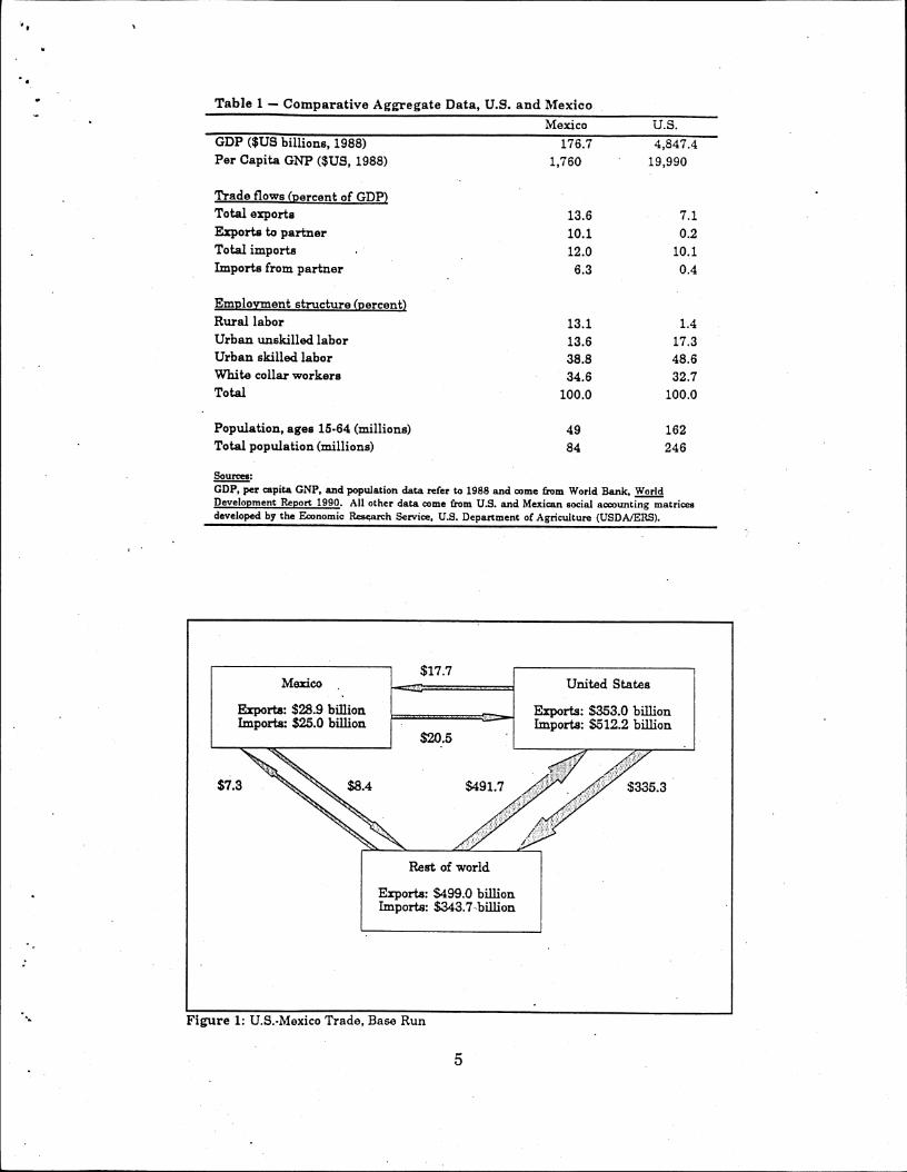
Table 1 - Comparative Aggregate Data, U.S. and Mexico

Mexico U.S.GDP ($US billions, 1988)Per Capita GNP ($US, 1988)

Trade flows (percent of GDP)Total exportsExports to partnerTotal importsImports from partner

Employment structure (percent)Rural laborUrban unskilled laborUrban skilled laborWhite collar workersTotal

Population, ages 15-64 (millions)Total population (millions)

176.7 4,847.4

1,760 19,990

13.6

10.1

12.0

6.3

13.1

13.6

38.834.6

100.0

7.1

0.2

10.1

0.4

1.417.3

48.6

32.7

100.0

49 162

84 246

Sources:GDP, per capita GNP, and population data refer to 1988 and come from World Bank, WorldDevelopment Report 1990. All other data come from U.S. and Mexican social accounting matricesdeveloped by the Economic Research Service, U.S. Department of Agriculture (USDA/ERS).

Mexico .

Exports: $28.9 billionImports: $25.0 billion

$17.7

$20.5

United States

Exports: $353.0 billionImports: $512.2 billion

$7.3 $8.4 $491.7 A $335.3

Rest of world

Exports: $499.0 billionImports: $343.7-billion

Figure 1: U.S.-Mexico Trade, Base Run

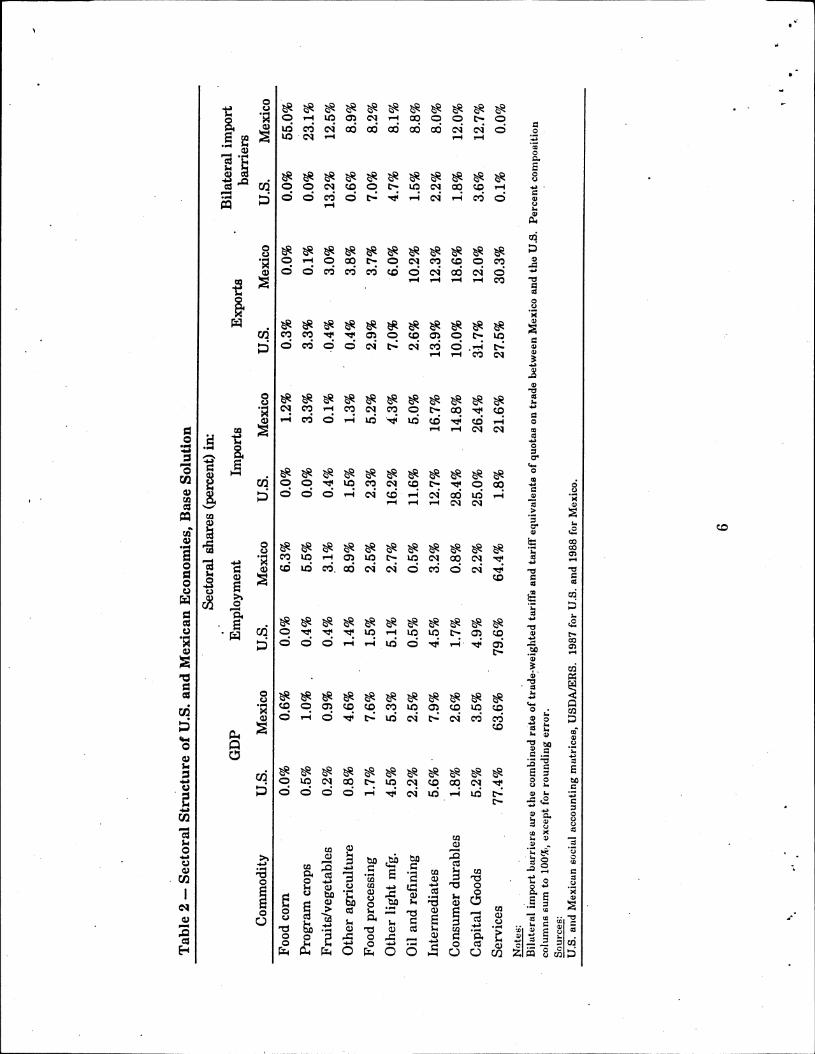
Table 2 - Sectoral St

ruct

ure of U.S. and Mexican Economies, Base Solution

Commodity

Sectoral sha

res (p

erce

nt) i

n:Bi

late

ral import

GDP

Employment

Imports

Exports

barriers

U.S.

Mexi

co

U.S.

Mexico

U.S.

Mexi

co

U.S.

Me

xico

U.S.

Me

xico

Food cor

n 0.0%

0.6%

0.0%

6.3%

0.0%

1.2%

0.3%

0.0%

0.0%

55.0%

Program cro

ps

0.5%

1.0%

0.4%

6.5%

0.0%

3.3%

3.3%

0.1%

0.0%

23.1%

Fruits/vegetables

0.2%

0.9%

0.4%

3.1%

0.4%

0.1%

.0.4%

3.0%

13.2%

12.5%

Other ag

ricu

ltur

e 0.8%

4.6%

1.4%

8.9%

1.5%

1.3%

0.4%

3.8%

0.6%

8.9%

Food processing

1.7%

7.6%

1.5%

2.5%

2.3%

5.2%

2.9%

• 3.7%

7.0%

8.2%

Other light mf

g.

4.5%

5.3%

5.1%

2.7%

16.2%

4.3%

7.0%

6.0%

4.7%

8.1%

Oil and ref

inin

g 2.2%

2.5%

0.5%

0.5%

11.6%

5.0%

2.6%

10.2%

1.5%

8.8%

Intermediates

5.6% •

7.9%

4.5%

3.2%

12.7%

16.7%

13.9%

12.3%

2.2%

8.0%

Consumer durables

1.8%

2.6%

1.7%

0.8%

28.4%

14.8%

10.0%

18.6%

1.8%

12.0%

Capi

tal Goods

5.2%

3.5%

4.9%

2.2%

25.0%

26.4%

31.7%

12.0%

3.6%

12.7%

Services

77.4%

63.6%

79.6%

64.4%

1.8%

21.6%

27.5%

30.3%

0.1%

0.0%

Notes:

,Bilateral import barriers ar

e the combined rat

e of

trade-w

eigh

ted ta

riff

s and tariff equivalents of quotas on trade between Mexico and the U.S

. Percent composition

columns stun to 100%, exc

ept for rounding err

or.

Sources:

U.S.

and Mexican soc

ial ac

coun

ting

matrices, USDAJERS. 1987 for U.S

. and 1988 for

Mexico.

6

„.

2 yellow corn imports from the U.S., which are assumed to enter food use. In the U.S., the

corn sector refers to No. 2 yellow corn, which exports to Mexico. The composition of the

program crops sector corresponds to the other crops eligible for U.S. deficiency payments --

feed corn, food grains, soybeans, and cotton. Other agriculture includes livestock, poultry,

forestry and fishery, and other miscellaneous agriculture. The fruits and vegetables sector

in Mexico includes beans, a major food crop.

There are six primary factors, including four labor types, capital, and agricultural

land. The four labor types are rural, urban unskilled, urban skilled, and professional. The

base year for Mexico is mostly 1988.3 The U.S. uses a 1987 base year because of the severe

contraction of agricultural output following the 1988 drought. Bilateral trade flows are from

1988. Because of the volatility in U.S. 1987-88 agricultural output, the model follows Adams

and Higgs (1986) and Hertel (1990) in the use of a "synthetic" base 'year for the U.S.,

imposing 1988 U.S.—Mexican bilateral trade flows on a 1987 base U.S. economy. This

approach has the advantage of achieving a more representative U.S. base year, with minimal

adjustment to the data.4 Tariffs and tariff equivalents of quotas are 1988 trade-weighted

rates.

The core model follows the standard theoretical specification of trade-focused CGE

models.5 Each sector Produces a composite commodity that can be transformed according

3The data base is documented in Burfisher, Hinojosa, Thierfelder, and Hanson (1991). Some of theMexican agricultural support data refer to 1989. The Mexican agricultural programs have changeddramatically over the past few years, and it is important to use the latest data available.

4A comparison of 1987 and 1988 U.S.-Mexico trade shows that Mexican farm imports increased in1988 as U.S. agricultural output fell. Use of a 1987/88 split year for the U.S. moderates theimportance of Mexico in U.S. agricultural trade relative to 1988.

6See the appendix for a complete equation listing. Robinson (1989) and de Melo (1988) surveysingle-country, trade-focused, CGE models. The FTA-CGE model is implemented using the GAMSsoftware, which is described in Brooke, Kendrick, and Meeraus (1988).

7

to a constant elasticity of transformation (CET) function into a commodity sold on the

domestic market or into an export. Output is produced according to a CES production

function in primary factors, and fixed input-output coefficients for intermediate inputs. The

model simulates a market economy, with prices and quantities assumed to adjust to clear

markets. All transactions in the circular flow of income are captured. Each country model

traces the flow of income (starting with factor payments) from producers to households,

government, and investors, and finally back to demand for goods in product markets.

Consumption, intermediate demand, government, and investment are the four

components .of domestic demand. Consumer demand is based on Cobb-Douglas utility

functions, generating fixed expenditure shares. Households pay income taxes to the

government and save a fixed proportion of their income. Intermediate demand is given by

fixed input-output coefficients. Real government demand and real investment are fixed

exogenously.

In factor markets, full employment for all labor categories is assumed. Aggregate

supplies are set exogenously. The model can incorporate different assumptions about factor

mobility. In the experiments reported here, we assume that agricultural land is immobile

among crops, but that all other factors are mobile, including capita1.6 The results should be

seen as reflecting adjustment in the long-run, with capital able to leave the agricultural

sectors.

There are three key macro balances in each country model: the government deficit,

aggregate investment and savings, and the balance of trade. Government savings is the

difference between revenue and spending, with real spending fixed exogenously but revenue

••••

Note, however, that labor markets are segmented. Rural labor does not work in the industrialsectors, and urban labor does not work in agriculture. These labor markets are linked throughseparate migration equations.

8

depending on a variety of tax instruments. The government deficit is therefore determined

endogenously. Real investment is set exogenously, and aggregate private savings is

determined residually to achieve the nominal savings-investment balance.7 The balance of

trade for each country (and hence foreign savings) is set exogenously, valued in world prices.

Each country model solves for relative domestic prices and factor returns which clear

the factor and product markets, and for an equilibrium real exchange rate given the

exogenous aggregate balance of trade in each country. The GDP deflator defines the

numeraire in each country model, and the currency of the rest of the world defines the

international numeraire. The model determines two equilibrium real exchange rates, one

each for the U.S. and Mexico, which are measured with respect to the rest of the world. The

cross rate (U.S. to Mexico) is implicitly determined by an arbitrage condition.

The model specifies sectoral export supply and import demand functions for each

country, and solves for a set of world prices that achieve equilibrium in world commodity

markets. At the sectoral level, in each country, demanders differentiate goods by country of

origin and exporters differentiate goods by country of destination.

3. Import Demand Equations

The standard approach in "Armington" trade models is to specify a constant elasticity

of substitution (CES) import aggregation function.8 In the case of a multi-country model, the

7Enterprise savings rates are assumed to adjust to achieve the necessary level of aggregate savingsin each country.

eThe properties of CGE models incorporating CES import aggregation functions have beenextensively studied. See, for example, de Melo and Robinson (1989) and Devarajan, Lewis, andRobinson (1990).

function aggregates imports from all countries of origin. In the simplest case, the CES

function is extended to include goods from many countries, with the substitution elasticity

assumed to be the same for all pairwise comparisons of goods by country of origin.9 The

first-order conditions define import demand as a function of relative prices and the elasticity

parameter. In our model, with three countries of origin, there are fifteen prices associated

with each sector in each country of destination, including the prices of the CES and CET

aggregates.

As noted earlier, the use of CES functions in multi-country Armington trade models

has led to empirical problems due to the restrictive nature of the CES functions. Instead of

the CES import aggregation function, we use import demand equations based on the Almost

Ideal Demand System (or AIDS).1° The AIDS function is a flexible functional form in that

it can generate arbitrary values of substitution elasticities at a given set of prices, and also

allows expenditure elasticities different from one.

In the AIDS approach, the expenditure shares are given by:

c1/4k,c1 E j,k,a,c2log(PM j,k,c2) + j,k,ci logS i,k,c1 e2

( 1 )

where subscript i refers to sectors; subscript k refers to the U.S. and Mexico; and subscript

cl refers to the U.S., Mexico, and the rest of the world. Si,k,ci is the expenditure share on

90ther generalizations of the CES function could allow different, but fixed, elasticities ofsubstitution between goods from different countries. See, for example, the CRESH function describedin Dixon et al. (1982). It is also common to use nested CES functions, with a two-good CES functionspecifying substitution between domestically produced goods and a composite of imports, which is itselfa CES function of goods from various countries of origin.

•

1°The AIDS specification in this model draws heavily on work by Robinson, Soule, and Weyerbrock(1991). The discussion below is based on their paper.

10

imports of good i into country k from country cl. oi,k is nominal expenditure on composite

good i in country k, P_ Mi,k,c2 is the domestic price of imports, and P is the aggregate price

of the composite good. The Greek letters are parameters.

We adopt the notation convention that when k = cl,

Mi,k,k= D1,k1 PMi,k,k = PDi,k and Si,k,k = PDio, • Di,k/ Ci,k

where Mi,k4 is the import of good i into country k from country cl, Di,k is the domestically

produced good sold on the domestic market, and PDi,k is the price of Di,k. Deaton and

Muellbauer (1980) define the aggregate price index, Pi,k, by a translog price index. In

econometric work, the translog price index is often approximated by a geometric price index

— a procedure we have followed in the results presented below.'

Various restrictions on the parameters are required to have the system satisfy

standard properties of expenditure functions such as symmetry, homogeneity, adding up, and

local concavity. We calibrated the parameters for the FTA—CGE model by starting from a

set of expenditure elasticities and substitution elasticities for each sector in each country.

We assumed that substitution elasticities are the same for goods from any .pair of countries,

so our AIDS functions are effectively simple extensions of the multi-country CES functions

to include expenditure elasticities different from one.12

"The geometric price index is usually called a Stone index. Robinson, Soule, and Weyerbrock(1991) analyze the empirical properties of different import aggregation functions in a three-countrymodel of the U.S., European Community, and rest of world, which is a close cousin of the FTA—CGEmodel. Green and Alston (1990) discuss the computation of various elasticities in the ADDS systemwhen using the Stone or translog price indices.

12We drew on work at the International Trade Commission for estimates of the various elasticities.See Reinert and Shiells (1991) who present estimates of substitution elasticities. They are currentlyworking on estimating AIDS functions.

11

4. Migration

The FTA—CGE model specifies three migration flows: rural Mexico to rural U.S. labor

markets, urban unskilled Mexico to urban unskilled U.S. labor markets, and internal

migration within Mexico from rural to unskilled urban labor markets. Migration is assumed

to be a function of wage differentials between the two countries. In equilibrium, migration

levels are determined which maintain a specified ratio of real wages, wgdfinig, for each labor

category in the two countries, measured in a common currency, and a specified ratio of.real

wages between the rural and unskilled urban markets in Mexico:

EXR.

""Nig̀mx = wgdfinig • FVFnuex • EXR.(2)

where the index mig refers to the three migration flows, WF is the wage, and EXR is the

exchange rate. The domestic labor supply in each skill category in each country is then

adjusted by the migrant labor flow.

An implication of this specification of migration flows is. that real wages measured in

a common currency are equated, but they can grow at different rates measured in the

domestic currency. It is therefore possible to observe migrants moving from a labor market

where real wages are rising to one in which they are falling in domestic currency terms. The

issue is in the specification of what motivates migrants. For example, if they are motivated

by the desire to accumulate savings which they intend to repatriate, then migration will be

sensitive to the exchange rate. On the other hand, if they are motivated by observations on

relative changes within the two economies then migration could be expected to be insensitive

to the exchange rate. The model probably overstates the sensitivity of migration to the

12

•••

exchange rate, generating a backward flow of migrants into Mexico when the Mexican peso

appreciates.

Migration flows generated by the FTA—CGE model refer to changes in migration from

a base of zero. They should be seen as additional migration flows due to the policy change,

adding to current flows. Current migration flows are substantial, both within Mexico and

between Mexico and the U.S.13 In addition, the net migration flows generated by the model

represent workers, or heads of households. In recent years, a substantial share of migrants

have been family members. The model thus probably understates total increased migration

due to a policy change, since family members will tend to migrate with workers.

5. Agricultural Programs

In both the U.S. and Mexico, the agricultural sector is characterized by a complex set

of trade policies and domestic agricultural programs. These policies distort production,

consumption and trade, and require significant fiscal expenditures in both countries. Tables

3 and 4 present data on their agricultural program expenditures in the base year. Mexican

agricultural program expenditure in 1988, totaling $1.6 billion, represented over one-half of

total national subsidy expenditure, and equaled almost one percent' of GDP.14 In the U.S.,

deficiency payments and expenditures on the export enhancement program (EEP) in 1987

totalled $11.5 billion, or one percent of government spending and 10 percent of the fiscal

deficit.

• 13Various researchers have placed the net increase of undocumented Mexican immigrants in theU.S. to be around 100,000 a year during the 1980s. See Bean, Edmonston, and Passel (1990).

14mi-ims total represents agricultural expenditures for 1989 and subsidies to food processing for 1988.

13

Table 3- Mexican Agricultural Program Expenditures

Subsidy

Other Fruits & Other Foodprogram vege- agri- proces-

Food corn crops tables culture sing Total •

- - - Billion Pesos • -.Credit (CSUB) 169.4 183.8 78.1 44.2 0.0 475.4Fertilizer (FSUB) 77.4 217.8 18.0 0:0 0.0 313.2Insurance (INSUB) 138.4 293.7 16.9 0.0 0.0 448.9Irrigation (IRSUB) 189.4 533.2 44.1 0.0 0.0 766.6Feed (FDSUB) 0.0 0.0 0.0 31.7 0.0 31.7Direct payment (DSUB) 0.0 0.0 0.0 0.0 325.1 325,1Price (PSUB) 0.0 0.0 0.0 0.0 . 1,085.1 1,085.1Tortilla (LOSUB) 0.0 0.0 0.0 0.0 223.8 223.8

Total (billion pesos) 574.6 1,228.4 157.0 75.9 1,633.9 3,669.9Total ($US millions) $253.1 $541.1 $69.2 $33.4 $719.8 $1,616.7Producer incentiveequivalent (PIE), % 16.4% . 20.8% 3.1% 0.2% . 0.4%Notes:"Food Corn" refers to corn used for human consumption (85% of total corn output). "Fruits & vegetables" includes beans(frijoles). CSUB, FSUB, INSUB, IBSUB, and FDSUB refer to 1989. DSUB, PSUB, and LOSUB refer to 1988. The PIErates are given ad valorem, although they are modelled as specific subsidies (per unit output).Source:Burfisher, et al. (1991).

Table 4 - U.S. Agricultural Program Expenditures

Otherprogram

Food corn crops Total

- - $ billion - - -Deficiency payments 0.76 9.85 10.62Export Enhancement Program (EEP) 0.00 0.88 0.88EEP for exports to Mexico 0.00 0.03 0.03

Total 0.76 10.74 11.50Producer incentive equivalent (PIE), % 18.7% 18.8%Notes:Programs include deficiency payments and the Export-Enhancement Program (EEP) for wheat in 1987.EEP payments for exports to Mexico refer to 1988."Food corn* refers to No. 2 yellow corn. Deficiency payments for food corn are computed as a share of totaldeficiency payments. The share of No. 2 corn exported to Mexico as a share of total corn output (11%).PIE rates are given ad valorem, although they are modelled as specific rates (per unit ouput).Sources:Agricultural Outlook, April 1991 and unpublished USDA data.

14

Table 5 — How Agr

icul

tura

l Programs are Modeled

Program ins

trum

ents

: Program:

Fixe

d Endogenous

United States

• Mexico

Price Wedges

PX, output pr

ice

PIE

Defi

cien

cy payment program

CSUB: cr

edit

FSUB: fe

rtilizer

INSUB: insurance

IRSUB: ir

rigation

FDSUB: fee

dDSUB: dir

ect

PD, domestic sales pr

ice

itax

it

ax: in

dire

ct tax

, psub

psub: pr

ice su

bsid

y •

PM, import pr

ice

tm

TM2

Tari

ffs and quotas on imp

orts

Ta

riff

s and quotas on

impo

rts

PE, export pr

ice

tee

. EEP: Export enhancement

program

PVA, val

ue added pri

ce

vatr

" Va

lue added tax

Income Tra

nsfe

rs

Hous

ehol

ds

losu

b losub: low

income tortilla

subsidy

Notes:

PIE refers to "producer incentive equ

ival

ent.

". In

the

mod

el, the PIE variable equals the sum of all pr

ice -we

dge in

stru

ment

s that affect th

eou

tput

pri

ce (PX

). T

ariff ra

tes,

tm, are fixed par

amet

ers.

The tar

iff equivalent of a quota, Tm

2, is

a variable determined endogenously, giv

enthe fi

xed import quota.

15

In the FTA—CGE model, agricultural policies are modeled either as price wedges,

which affect output decisions, or lump-sum income transfers. The wedges and transfers are

either specified exogenously or determined endogenously, based on the institutional

characteristics of the program being modelled. The various programs and how they are

treated in the model are summarized in Table 5.

Border policies (tariffs, quotas, and export subsidies) affect producers through their

effect on the output price, PX.i,k, which is effectively a weighted average of the prices of

output sold in the domestic market, PDi,k, and in each export market, PEi,k,ci. Similarly, they -

affect consumers through the price of the composite good, Pi,k, which is effectively a weighted

average of the domestic currency price of. the imported good, PMi,k, and the domestic good

price, PDLk." Given the CET and AIDS functions, the link between trade policy and

domestic prices is weaker than in a model where all goods are perfect substitutes.

5.1 Mexican Agricultural Programs

Six Mexican policies are modeled.' In the four agricultural sectors, these are input

subsidies, tariffs, and quotas. In the food processing sector, we model direct subsidies and

price subsidies, in addition to tariffs and quotas. The sixth Mexican policy is the low income,

or tortilla, subsidy.

Mexico provides its farmers with input subsidies on credit, fertilizer, insurance,

irrigation, and feed. Input subsidies are represented in the model as a per-unit mark-up on

15-PX is a CET aggregation of PD and PE, while P is a translog or Stone aggregation of PD andPM.

16Mexican agricultural policies are described in Krissoff and Neff (1992); Burfisher (1992); Mielke(.1989, 1990); O'Mara and Ingco (1990); and Roberts and Mielke (1986).

16

output price measured as a fixed number of pesos per unit of output.17 Reflecting their

effect on the producer's output decision, input subsidies are summed into a Producer

Incentive Equivalent (PIELk), in pesos per unit of output. For the U.S. and Mexico, the

producer incentive equivalents in ad vczlorem terms range from 16 to 21 percent (Tables 3 and

4). Given the assumption of fixed input-output coefficients, the profit maximization problem

uses the value added-price (PVALk) in computing the marginal revenue product as an

argument to determine demand for primary factors; PVA is the price received by producers

(PX, defined net of indirect taxes), minus the cost of intermediate inputs (given by input-

output coefficient, I0j,i,k), and plus all subsidies (PIE):

PVAi, = PX - E 1A P. ) + PIEiok (3)k i,k ,1

Increasing the producer's value-added price with a positive PIE increases factor returns and

induces a resource pull of factors toward the subsidized sector, causing output in the sector

to expand.

Import quotas in agriculture are used by the Mexican government as a supply

management tool to maintain targeted domestic farm prices. Import licenses are generally

issued after the domestic crop has been harvested and purchased. To acquire a license,

private importers or. Mexico's food parastatal, the Compania Nacional de Subsistencias

Populares (CONASUPO), must show that domestic supplies are being purchased for not less

than the government target price. Mexico is assumed to be a small country in the world

market for its agricultural imports, so that their quotas do not affect the world price. The

17Input subsidies can be tied directly to output because intermediate demand is modeled with fixedinput-output coefficients. With more complex production functions, input subsidies should be directlytied to input usage. A "u" as the final letter in the name of a subsidy signifies that it is provided perunit of output.

17

tariff equivalent of the quota, TM2i,k,ci, can be calculated as the "price-gap" between the

world price and the domestic price. Following Dervis, de Melo, and Robinson (1982) and

Kilkenny (1991), TM2i,k,c, is determined endogenously, so that the quota's ad valorem

equivalent (and hence the value to license holders of the import premia) changes with the

price gap.

Premium income from each sector is distributed to the holders of import licenses.

Since only Mexicans are awarded licenses, the rent is retained domestically. In the

FTA—CGE model, the rent is allocated between government revenue and enterprise income

according to the share of the government and private sector in imports.18 Tariffs are

modelled with fixed ad valorem rates, and tariff revenues are paid by consumers to

the government.

Since December 1987, Mexico has placed price controls on almost all basic foods,

including corn products, wheat products, dairy, eggs, poultry, and pork. To enable food

processors to sell their output at low consumer prices fixed by price controls, the government

offsets processors' high input prices with two types of subsidies. One is a direct subsidy,

DSUBLk. This is a modeled as a fixed budgetary transfer from the government to the

processing sector, with a unit value (DSUBUi,k) that varies with a change in output:

DSUBiDSUBU - ,k (4)

XD

DSUBULk is included in the PIELk price wedge on producer's value-added price, and the direct

subsidy expenditure is treated as a fixed component of Mexican farm program expenditures.

18Tariffs and quotas are modelled identically for the U.S. and Mexico, except that in the U.S.,quota premia accrue to capital income.

18

The Mexican government also provides processors with an input price subsidy,

PSUBi,k, to compensate them for the high purchase price of domestic agricultural inputs, and

to enable them to sell their output on the domestic market at the controlled retail price Pi,k.

PSUBULk is the input price subsidy in pesos per unit of output. Its initial value is calculated

from data on sectoral government expenditures on price subsidies, PSUBi,k, and domestic

sales, DI ,k as:

PSUB1,kPSUBUik D

(5)

Price subsidies increase a processor's domestic sales price tO PDAi,k, the actual"

domestic sales price received by each producer:

PDAI,k = PD, + PSUBU,k (6)

In a model with more sectoral disaggregation, the unit price subsidy should be

modeled endogenously as the price wedge on a processor's domestic sales price that is

required to maintain the fixed retail price of the composite good, Pi,k. Because the 11-sector

model aggregates all food processing into a single sector, PSUBUi,k is represented as a fixed

price wedge and consumer food prices are permitted to vary. Quota removal under an FTA

is simulated by simply removing the wedge, rather than allowing the model to determine the

change in PSUBUi,k. PSUBUi,k enters into PIEi,k where it affects each producer's value-

added price. The cost of the price subsidy to the government increases with an increase in

domestic sales, and is included in agricultural program expenditures.

Mexico provides low income consumers with subsidized corn tortillas. Under one

program, low prices are offered in CONASUPO-owned retail outlets located in low-income

neighborhoods. More recently, the government has provided low-income households with one

kg. per day of tortillas, approximately one-half the daily average household consumption

19

[Levy and van Wijnbergen, (1991)]. Since the FTA—CGE model has only a single aggregate

household, with no differentiation by income, the tortilla subsidy is represented as a lump-

sum income transfer to the single household. Similar to direct subsidies to processors,

expenditure by the government on low income corn subsidies, LOSUBLk, is fixed and enters

into Mexican agricultural program expenditures.

5.2 U.S. Agricultural Programs

Two U.S. farm programs could be affected by an FTA -- deficiency payments and the

EEP.19 The U.S. deficiency payments program provides payments to farmers who

participate in feed grain, wheat, rice, or cotton programs. The payment rate is calculated as

the difference between a fixed target price (TPi,k) and the market price (PX.i,k) or loan rate,

whichever difference is less. The total payment a farm receives (DEFPAYi,k) is the payment

rate multiplied by eligible base production (XPi,k):2o

DEFPA = TPi,k - PXj,k) (7)

The U.S. EEP program is intended to counter competitors' subsidies and other "unfair"

trade practices in targeted U.S. agricultural export markets,' and to develop, expand, or

maintain foreign markets. Under the EEP program, the USDA approves an initiative to

permit an importing country to tender for a specified quantity of a designated commodity.

190ur modeling of these programs in the FTA—CGE model follows Kilkenny and Robinson (1988,1990) and Kilkenny (1991).

20The initial value of the target price is calculated from base-year data on the aggregate cost ofdeficiency payment (DEFPAY) which is then used to estimate the mark-up on the market price. Themodel also implicitly fixes participation rates at the base year rate, implying that any increase in U.S.program crop output comes from outside the deficiency payments program. In recent years, themarket price has been above the loan rate, so we have not had to model the non-recourse loanprogram.

20

Exporting firms bid for the sale, which are contingent on receiving an EEP bonus from the

Commodity Credit Corporation (CCC). EEP bonuses are fungible, in-kind certificates backed

by commodities owned by the CCC. The firms estimate the per unit subsidy they will need

to complete the sale and then compete against each other for the EEP bonus. The CCC then

accepts one of the bids, based on the price and bonus ranges. In effect, the EEP program

works as an ad valorem export subsidy, which is how it is treated in the FTA-CGE model.

The subsidy rate, TEEi,k,ci, is applied as a mark-up on the world export price:

PE = PWEIAc1•EXRk•(1 + TEE11) (8)

which allows U.S. producers to lower the world price of their goods relative to other suppliers,

while maintaining their received price (PE). Total EEP expenditures are included in farm

program expenditures.

For each country, the policy-ridden, value-added producer price becomes:

[(1 - /TAX/A) •PDIA + PSUBUI 1-Da + E PEioka•EiAdPVAirt = cl

- E PlEisk

XDi,k (9)

where: ITAX is the indirect tax rate, PSUBU is the subsidy rate on domestic sales (by food

processors in Mexico), and PIE is a bundle of subsidies in domestic currency per unit of total

output (Table 5). The other variables are defined above.

Four types of elasticity parameters are used in the model. The production

specification requires sectoral elasticities of substitution among primary factors. The CET

export supply functions require elasticities of transformation between goods sold on the home

and export markets. The AIDS import demand functions require sectoral income elasticities

and substitution elasticities for home goods and for goods from each import source. We have

21

drawn on estimates. and "guesstimates" from various studies, including Hinojosa and

Robinson (1991.), Hanson, Robinson, and Tokarick (1989); and Reinert and Shiells (1991). In

lieu of econometric estimation, ensitivity analysis was carried out to check for the robustness

of the model results using alternative elasticity parameters.

6. Model Results

6.1 Scenarios

We analyze the effects of a U.S.—Mexico FTA under six scenarios, which are

summarized in Table 6. All the scenarios involve changes in policies between the U.S. and

Mexico, leaving unchanged their policies with respect to the rest of the world. The first

scenario is the removal of all non-agricultural protection between the U.S. and Mexico,

leaving all agricultural protection and programs intact. The second scenario is removal of

tariffs and quotas in all industrial and agricultural sectors, but again leaving all agricultural

programs, except for the removal of the U.S. EEP program with respect to Mexico.21 A

third scenario considers trade and agricultural liberalization, removing all Mexican subsidies

to farmers and food processors, in addition to full trade liberalization. .We also ran a variant

of Scenario 3, 3a, in which input subsidies to the food corn sector were eliminated, but all

21u.n.quotas on sugar imports (in the processed food sector) were also left intact. As a net sugarimporter, Mexico is unlikely to become a sugar exporter to the U.S. under an FTA, except insofar asit attempts to increase its quota rents from arbitrage sales to the U.S. market. In any event, tradein sugar and items of high sugar content was not liberalized under the U.S.—Canada FTA, and islikely to be excluded from the U.S.—Mexico FTA.

22

Table 6 — Description of Scenarios

No. Scenario Description

1. Industrial tradeliberalization

2. Trade liberalization

3. Trade and Mexicanagricultural liberalization

3a. Trade and Mexican cornliberalization

4. Trade liberalization pluscommon agriculturalpolicies

5. Partial trade liberalization

6. Partial liberalization pluscapital growth in Mexico

Remove all non-agricultural tariffs and quotas.

Remove all tariffs and quotas. Remove U.S. EEPprogram subsidizing exports to Mexico.

Scenario 2 plus eliminate all agricultural supportprograms in Mexico.

Scenario 2 plus eliminate input subsidies for cornsector in Mexico.

Scenario 2 plus add a deficiency payment programfor corn and other program crops in Mexico.

Tariffication of Mexican agricultural import quotasat 50% of tariff equivalent. Add deficiencypayment program to Mexico in corn. Leave allexisting agricultural programs intact.

Tariffication of Mexican agricultural import quotasat 50% of tariff equivalent. Mexican capital stock10% higher. Mexican agricultural subsidies (PIE)cut in half for corn and other program crops. Nodeficiency payment program in Mexico.

23

other Mexican agricultural programs remained intact.22 The fourth and fifth scenarios

explore the effects of restructuring Mexican domestic agricultural policies in conjunction with

an FTA. In the fourth scenario, in addition to full U.S.—Mexico trade liberalization, Mexico

adopts a deficiency payments program for corn and program crops similar to the U.S.

program and continues its farm and food processing subsidies. This mix of policies has the

effect of protecting Mexican producers through domestic programs rather than trade barriers.

In the fifth scenario, a deficiency payments program is combined with the tariffication of

Mexican quota protection in the corn and program crops sectors at one-half the level of the

tariff equivalents of base year quotas. This partial trade liberalization scenario reduces .the

fiscal burden of protecting Mexican producers because some tariff barriers are maintained.

In the sixth scenario, the Mexican aggregate capital stock is assumed to be augmented by

10 percent, simulating the effects of the anticipated increased capital inflows under an FTA,

which should lead to Mexican growth relative to the U.S.

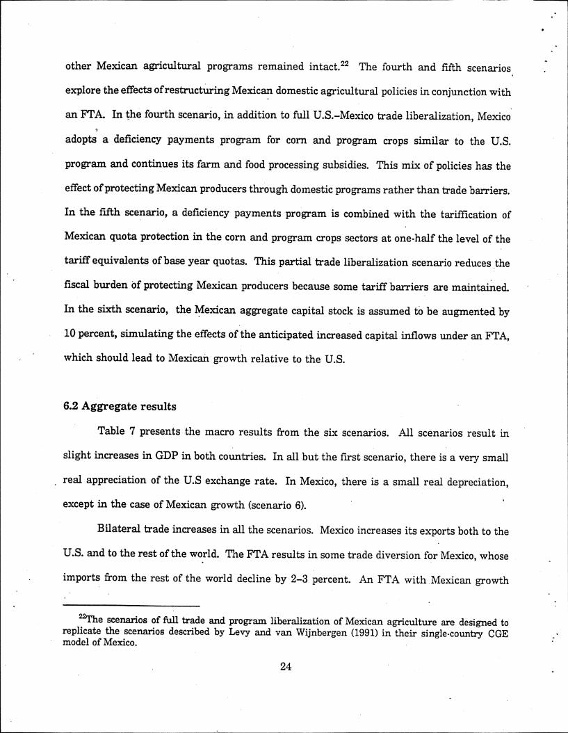
6.2 Aggregate results

Table 7 presents the macro results from the six scenarios. All scenarios result in

slight increases in GDP in both countries. In all but the first scenario, there is a very small

real appreciation of the U.S exchange rate. In Mexico, there is a small real depreciation,

except in the case of Mexican growth (scenario 6).

Bilateral trade increases in all the scenarios. Mexico increases its exports both to the

U.S. and to the rest of the world. The FTA results in some trade diversion for Mexico, whose

imports from the rest of the world decline by 2-3 percent. An FTA with Mexican growth

22The scenarios of full trade and program liberalization of Mexican agriculture are designed toreplicate the scenarios described by Levy and van Wijnbergen (1991) in their single-country CGEmodel of Mexico.

24

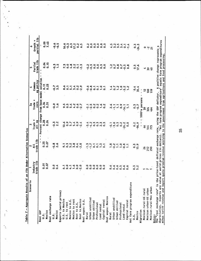
Table 7 - Aggregate Results of an ETA Under Alternative Scenarios

Scenario

1 2

3

3a

4

5

6Industry

All

Trade +

Common

Partial

Grow

th +

trad

e lib

part

ial

lib

trade l

ib

trad

e lib

all ag

TCC:111+

ag po

licy

Re

al GDP

- - -

Percent change from base model solution -

- -

11

.0

,U.S.

0.01

0.23

0.28

0.34

. 0.04

0.00

Mexico

0.07

0.27

. .

0.24

0.31

0.23

0.15

7.43

Real exchange rate

U.S.

0.0

-0.8

-0.3

-0.9

-0.7

-0.3

-0.6

Mexi

co

0.4

2.6

2.2

1.6

3.5

1.5

-0.5

Exports (world prices)

U.S. to Me

xico

6.1

9.1

10.6

9.5

8.6

7.3

16.6

U.S. to rest

0.0

0.3

0.9

0.5

0.1

0.0

-0.3

Mexi

co to U.S..

4.1

5.2

5.7

5.4

5.1

4.8

6.3

Mexico to rest

1.6

3.8

5.4

4.2

3.4

2.2

17.2

Rest to U.S.

0.0

0.4

0.9

0.6

0.2

0.1

0.2

Rest to.Mexico

-2.0

. -2.8

-2.4

-2.7

-2.9

-2.3

6.5

Real wages: U.S.

Rural

0.0

-1.3

-3.4

-2.1

-0.6

-0.2

0.2

Urban un

skil

led

0.0

-1.7

-4.2

. -2.5

-0.8

-0.3

0.0

Urban skilled

- 0.0

0.1

0.3

0.2

0.1

0.0

0.0

Professional

0.0

0.1

0.3

0.2

0.1

0.0 .

0.0

Land

re

ntal

0.0

1.3

2.3

1.6

1.0

0.3

0.8

.Ca

pita

l rental

0.0

0.1

0.3

0.2

0.1

0.0

0.0

Real wages: Mexico

Rura

l 0.6

. 1.8

-0.1

2.6

1.4

1.2

4.5

Urban uns

kill

ed

0.6

-0.2

-3.0

-1.1

0.7

0.7

3.2

.

Urban skilled

0.6

1.1

0.3

1.1

1.2

0.8

3.5

Professional

0.5

1.0

0.2

0.9

1.0

0.7

3.4

Land r

ental

0.6

-8.8

-24.

2 -1

4.1

-3.2

-0.5

0.1

Capital

rental

0.6

1.1

0.0

1.1

1.2

0.8

-1.4

Net farm program expenditure

U.S.

0.3

0.3

0.2

0.3

'0.4

0.5

0.3

Mexico

5.2

15.9

-96.9

- -0.7

35.4

17.6

-24.3

Migration

_ _ 7 10

00's

persons _

_ _

Mexi

can

rural-US r

ural

1 26

66

39

12

4

0Mexican urban-US urban

7

212

544

324

100

39

-2

Mexican

rural-Mex

urban

1 290

773

464

119

40

21Notes:

The 'real exchange rate" is the price-level de

flat

ed exc

hang

e rate, using

the GDP deflator. A positive change represents a

depreciation.

.Exports are value at wo

rld prices (in dol

lars

).

Net farm program exp

endi

ture

' equals farm program ex

pend

itur

esminus tariff revenue and import quo

ta premium revenue accruing to the government from agriculture and

food processing.

25

(scenario 6), however, does result in an increase of imports from the rest of the world. An,

FTA is trade creating for the U.S., with U.S. imports increasing from both Mexico and the

rest of the world in all scenarios. The Mexican growth scenario results in a slight diversion

of U.S. exports away from the rest of the world as part of a large increase in U.S. exports to

Mexico. This result emphasizes the importance of investment growth in Mexico in

determining the overall benefits of an FTA for the U.S.

Sectoral results are given in Tables 8a and 8b. U.S. export growth to Mexico is

highest in the agricultural sectors where Mexican protection has remained relatively high.

U.S. export growth corresponds to the decline in Mexican food corn and program crop output

under all five agricultural trade and liberalization scenarios. Full liberalization of the

Mexican food corn sector (scenarios 3 and 3a) result in a nearly 20 percent fall in output

while U.S. food corn output rises about 5 percent and exports to Mexico soar by almost 200

percent.

Mexico's fruit and vegetable sector undergoes less spectacular yet significant export

growth (ranging from 18 percent to 21 percent) under an FTA which includes agriculture,

reflecting the high initial U.S. tariff rates in this sector. Trade liberalization leads to a

significant increase in two-way trade in fruits and vegetables, with exports expanding in both

countries. Mexican fruit and vegetable output expands, while U.S. output hardly changes.

A policy mix in Mexico that maintains some trade barriers for agriculture (scenario 5) results

in much lower, although still significant, growth in U.S. exports of corn and program crops

to Mexico.

26

•

Table 8a - Sectoral Results, Scenarios 1 - 3a

Scenario

1

2

3

3a

Indu

stry

trade lib

All trade lib

Trade + all

ag

Trade + corn

Output

Expo

rts

Output

Expo

rts

Output

Exports

Output

Expo

rts

United Sta

tes

- - - Pe

rcen

t change from bas

e model solution - - -

Food corn

0.0

-1.0

4.1

156.

0 5.

1 18

5.4

5.3 .

196.3

Program cro

ps

0.0

-0.4

0.

8 40

.5

1.7

88.2

1.0

39.2

Frui

ts/v

eget

able

s 0.0

-0.7

0.1

14.2

0.7

13.6

0.2

14.0

Other agriculture

0.0

-0.4

0.

2 8.

3 0.6

6.8

0.4

8.2

Food processing

0.0

6.6

0.3

6.3

0.7

5.7

0.4

6.4

Other lig

ht mfg.

0.0

6.4

0.2

6.0

0.5

6.0

0.3

6.2

Oil & ref

inin

g 0.

0 13

.8

0.0

13.9

- 0.0

13

.9

0.0

14.0

Intermed

iate

s 0.

0 4.

8 0.

2 4.

7 0.5

4.7

0.3

4.9

Consumer durables

0.2

11.2

0.3

10.8

0.7

10.8

0.

4 10.9

Capi

tal go

ods

0.0

4.7

0.2

4.7

0.5

4.6

0.3

4.7

Services

0.0

-0.4

0.2

-0.8

0.6

-1.0

0.

4 -0.7

Mexico

Food cor

n -0.1

0.0

-10.

2 0.0

-19.

4 0.0

-19.1

0.0

Program cro

ps

0.2

0.0

-7.1

0.0

-21.

1 0.0

-6.7

0.0

Frui

ts/v

eget

able

s 0.

0 0.3

5.3

19.1

3.

1 17.6

6.1

20.8

Other agriculture

0.0

0.3

0.9

3.0

-1.3

1.8

1.0

3.4

Food processing

0.0

13.4

0.9

11.0

-2

.0

7.1

0.9

10.9

Other lig

ht mfg.

0.7

9.2

0.9

10.5

1.2

11.8

1.0

10.8

Oil & ref

inin

g 0.

0 3.

7 0.0

3.7

0.0

3.7

0.0

3.6

Intermediates

0.2

2.9

0.4

3.7

0.7

4.8

0.5

4.0

Consumer durables

1.0

3.9

2.4

5.4

4.5

7.5

2.7

5.7

Capi

tal go

ods

0.1

5.2

0.6

6.1

1.2

7.4

0.7

6.3

Serv

ices

-0.1

0.7

0.0

1.0

0.4

1.9

0.2

1.2

Notes:

Real

output and exp

orts

. Exports ar

e to the par

tner

cou

ntry

(U.

S. or Me

xico

).

27

•

Table 8h - Sec

tora

l Results, Scenarios 4 - 6

Scenario

4

5

6Common ag pol

icy

Partial trade lib

Growth + partial lib

Output

Expo

rts

Output

Expo

rts

Output

Expo

rts

United States

- - - Pe

rcen

t change from bas

e mo

del.

solution - - -

Food corn

3.3

128.0

1.2

49.0

2.6

100.

6Program crops

0.6

36.3

0.2

13.7

0.5

64.3

Frui

ts/v

eget

able

s -0.1

14.4

-0

.2

14.8

-0.3

26

.4Ot

her agriculture

0.1

8.3

0.1

8.6

0.0

17.8

Food processing

0.1

6.2

0.1

6.4

0.0

16.1

Othe

r light mfg.

0.1

5.9

0.0

6.2

-0.1

14.2

Oil & refining

0.0

13.8

0.0

13.8

0.0

23.0

Inte

rmed

iate

s 0.

1 4.

6 0.0

4.7

0.0

14.8

Consumer dur

able

s 0.

2 10

.8

0.2

11.0

0.1

14.0

Capital go

ods

0.1

4.6

0.1

4.6

0.0

10.5

Services

0.1

-0.8

0.0

-0.6

0.0

1.2

Mexi

co

Food cor

n -3

.1

0.0

-1.5

0.0

-4.5

0.0

Program crops

-6.0

0.0

-2.6

0.0

-3.6

0.0

Frui

ts/v

eget

able

s 4.

6 18

.0

4.2

17.4

8.1

17.4

Other agr

icul

ture

0.9

2.7

0.2

1.5

8.8

5.5

Food pro

cess

ing

0.9

11.0

0.3

8.7

9.5

17.4

Othe

r li

ght mfg.

0.8

10.2

0.

7 9.6

10.0

20.2

Oil & refining

0.0

3.7

0.0

3.7

0.0

-1.5

Inte

rmed

iate

s 0.3

3.5

0.2.

3.1

7.0

7.7

Consumer dur

able

s 2.1

5.1

1.4

4.3

12.2

12

.8Capital go

ods

0.5

5.9

0.2

5.4

6.0

11.5

Services

-0.1

0.8

-0.1

0.6

7.4

5.9

Notes:

Real output and exports. Exports are to the partner country (U.S. or Mexico). 28

6.3 Migration and. Farm Program Expenditure

Complete trade liberalization and the accompanying removal of subsidies to Mexican

agriculture and food industries (scenario 3) has a major effect on migration. About 12 percent

of Mexico's rural labor force (839,000 workers) migrate either to the U.S. or to Mexican urban

areas (Table 7). These workers come from the corn, program crop, and other agricultural

sectors, which contract sharply with quota and program removal. Expansion of fruit and

vegetable output, spurred by export growth to the U.S., is insufficient to absorb the displaced

agricultural workers. A total of 610,000 Mexican workers migrate to the U.S., 66,000

directly from the Mexican rural sector to the U.S. rural sector and another 544,000 urban

unskilled migrants moving to the U.S. from Mexican cities. There is a domino effect at work,

with rural-urban migration in Mexico leading, in turn, to migration from Mexico to U.S.

urban areas. Isolating the impact of Mexican food corn liberalization (scenario 3a) indicates

that about 60 percent of the total outmigration associated with complete agricultural trade

and program liberalization is due to liberalization of the corn sector.

In addition to large migration flows, scenarios 3 and 3a also generate the worst

distributional outcomes. Real wages of both rural and urban unskilled workers fall sharply

in the U.S., due to increased migration, and fall in Mexico for the same reason, although to

a lesser degree. Full trade liberalization and removal of agricultural programs in Mexico

yields a pattern of integration with lower wages for the poorest members of both societies.'

Scenarios 4 and 5 were designed to ameliorate the impact of trade liberalization on

Mexican migration. They are successful in reducing the migration flows, but they also

231n scenario 3a, the FrA—CGE model shows Mexican rural wages rising. This result is explainedby the large exodus of rural workers out of the food corn sector, while. the rest of the higher payingprogram crops continue to be supported. The Mexican government, however, has already begun to cutsupport for other program crops, leaving food corn relatively protected at this time.

29

increase Mexican agricultural program expenditures. Scenario 4, which adds a deficiency

payments program in Mexico similar to that in the U.S., supports the corn and program crop

output that had previously been supported by a quota. Mexican agricultural output falls only

slightly in these sectors, but Mexican agricultural imports from the U.S. still increase sharply

because removal of trade barriers lowers the relative price of imports. The deficiency

payments program leads to a much smaller increase in migration, but incurs a 35.4 percent

increase in Mexican net farm program expenditures (which take account of change in import

tariff and premium revenue, as well as budgetary outlays).

Scenario 5, which replaces agricultural quotas with tariffs set at half of the tariff

equivalents of base year quotas, supports the Mexican corn and program crop producer prices

and results in only a small contraction in output. Only 44,000 workers leave Mexican

apiculture. While scenarios 4 and 5 both reduce Mexican migration flows, the increase in

Mexican agricultural program expenditures is much lower when partial trade barriers are

maintained (scenario 5), increasing only 17.6 percent.

Scenario 6 results in very low Mexican migration flows and only a slight contraction

in output in the corn and program crops sectors (3-5 percent). Expansion of other sectors

absorbs Mexican rural labor and eliminates any new net increases in the migration flow to

the U.S. (indeed, reversing it by 2,000). Net agricultural program expenditures fall 24.3

percent, due both to decreased input subsidies and to increased tariff revenue. Scenario 6 is

the only agricultural liberalization FTA scenario where real wages rise for all labor groups

in both countries. This scenario indicates the importance to the success of the FTA for both

countries of Mexico achieving more rapid growth.

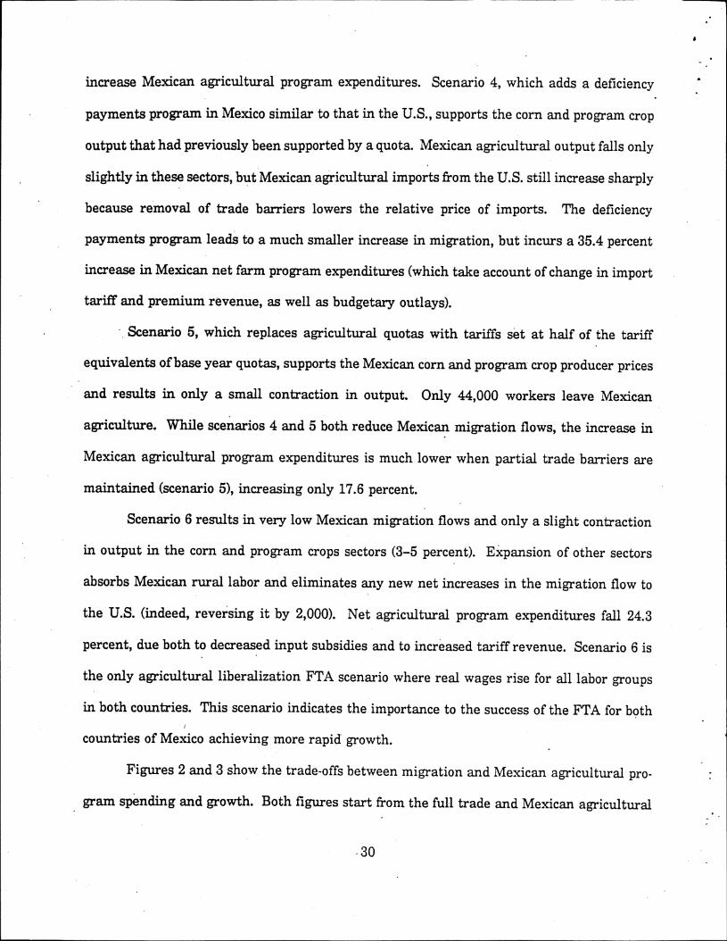
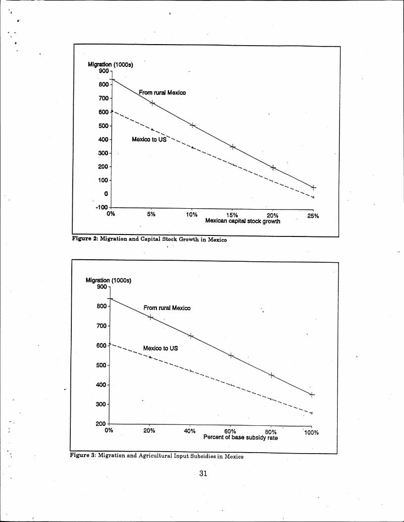
Figures 2 and 3 show the trade-offs between migration and Mexican agricultural pro-

gram spending and growth. Both figures start from the full trade and Mexican agricultural

30

• •

Migration (1000s)900 -

800

700

600

500

400

300

200

100-

0

-100

From rural Mexico

Mexico to US

0%

••••

51% 10% 15% 20% 2%Mexican capital stock growth

Figure 2: Migration and Capital Stock Growth in Mexico

Migration (1000s)900 -

800

700

600

500

400

300 -

200

From rural Mexico

Mexico to US

0%

S.

_

•••••••••,

26% 40% 60% 80% .1010%Percent of base subsidy rate

Figure 3: Migration and Agricultural Input Subsidies in Mexico

31

program liberalization (scenario 3) as their base. Figure 2 shows the sensitivity of different

types of migration to increased growth. In order to counteract completely the increases in

migration resulting from scenario 3, the Mexican capital stock would have to grow 25 percent

relative to the U.S. Figure 3 demonstrates the sensitivity of migration to spending on

agricultural input subsidies. With a 100 percent reinstatement of input subsidies, the level

of migration is close to that of scenario 2, which is still significant. It is interesting to note

that both for increased capital growth and agricultural support policies, the migration

relationship is almost linear. Each percentage point increase in the Mexican capital stock

reduces migration to the U.S. by roughly 25,000 workers and each percentage point increase

in agricultural input subsidies reduces migration by 3,500 workers.

7. Conclusion

This article analyzes the effects of a U.S.—Mexico free trade agreement using a multi-

country CGE model in which labor migration and domestic agricultural programs are

modeled explicitly, and a flexible functional form is used for import demand equations. The

model is used to analyze six scenarios. These represent complete bilateral trade liberalization

and Mexican agricultural program elimination; two combinations of Mexican agricultural pro-

grams that would reduce the labor migration caused by an FTA; and trade liberalization with

a capital inflow into Mexico.

Our results show that both countries achieve welfare gains Under an FTA, even in

scenarios in which some production and trade distorting policies are maintained. Bilateral

trade increases significantly with removal of trade barriers. An FTA is trade creating for

both countries in all scenarios, but some scenarios lead to trade diversion for Mexico, with

32

slightly reduced imports from the rest of the world. As Mexico grows, however, its trade with

both the U.S. and the rest of the world grows.

We show that alternative structures of FTA's generate trade-offs between the growth

in exports that is stimulated by lower trade barriers, versus the cost such liberalization

generates in agricultural program expenditures and new net increases in labor migration

flows. Free trade increases bilateral trade, but induces large rural outmigration from Mexico.

Mexico can reduce labor migration through the adoption of a deficiency payments program

that maintains agricultural income, but the fiscal effects are prohibitive. Retaining some

trade barriers in agriculture reduces bilateral trade growth, but also reduces migration and

growth in agricultural program expenditures. Increased capital inflows into Mexico result

in expanded bilateral trade, much lower migration flows, and a large reduction in Mexican

agricultural program expenditures. Dynamic effects are clearly very important in achieving

the full benefit of an FTA.

These findings suggest that Mexico will need a lengthy transition period and must

allocate resources to agriculture during the transition. Trade liberalization leads to an

immediate increase in rural outmigration, while the increased growth needed to absorb the

displaced labor takes longer. The rapid introduction of free trade in agriculture and the

elimination of agricultural support programs may not be desirable for either country when

the social and economic costs associated with increased migration are weighed against the

benefits of increased trade growth.

33

References

Adams, P.D. and P. J. Higgs (1986). "Calibration of Computable General EquilibriumModels from Synthetic Benchmark Equilibrium Data Sets." IMPACT PreliminaryWorking Paper No. OP-57, Melbourne, Australia.

Alston, Julian M., Colin A. Carter, Richard Green, and Daniel Pick (1990). "WhitherArmington Trade Models?" American. Journal of Agricultural Economics. Vol. 72,No. 2 (May), pp. 455-467.

Bean, Frank D., Barry Edmonston, and Jeffery S. Passel, eds. (1990). UndocumentedMigration to the United States: IRCA and the Experiences of the 1980s. Washington,D.C.:, The Urban Institute Press.

Brooke, Anthony, David Kendrick, and Alexander Meeraus (1988). GAMS: A User's Guide.Redwood City, CA: The Scientific Press.

Brown, Drusilla (1987). "Tariffs, Terms of Trade and National Product Differentiation."Journal of Policy Modeling (9): 503-526.

Burfisher, Mary. E. (1992). "The Impact of a U.S.—Mexico Free Trade Agreement on• Agriculture: A Computable General Equilibrium Model with Agricultural Trade

Policies and Farm Programs." University of Maryland, Ph.D. dissertation, CollegePark, Maryland, forthcoming.

Burfisher, Mary E., Raul Hinojosa-Ojeda, Karen E. Thierfelder, and Kenneth Hanson (1991)."Data Base for a Computable General Equilibrium Analysis of a U.S.—Mexico Freeih-acle Agreement." U.S. Department of Agriculture, Washington, D.C.

Deaton, Angus and John Muelbauer (1980). Economics and Consumer Behavior. Cambridge:Cambridge University Press.

Dervis, K., Jaime de Melo, and Sherman Robinson (1982). General Equilibrium Models forDevelopment Policy. Cambridge: Cambridge University Press.

Devarajan, Shantayanan, Jeffrey D. Lewis and Shserman Robinson (1990). "Policy Lessonsfrom Trade Focused, Two-Sector Models." Journal of Policy Modeling (12): 625-657.

Dixon, P.B., B. Parmenter, J. Sutton and D. Vincent (1982). ORANI: A Multi-sector Model of the Australian Economy. Amsterdam: North Holland.

Goodloe, Carol and John Link (1991). "The Relationship of a Canadian-U.S. TradeAgreement to a Mexican-U.S. Trade Agreement." Paper presented at the XXIImeeting of the International Association of Agricultural Economist's, Tokyo, Japan.

Green, Richard and Julian M. Alston (1990). "Elasticities in AIDS Models." American- Journal of Agricultural Economics. Vol. 72, No. 2 (May), pp. 442-445.

34

Hanson, Kenneth, Sherman Robinson, and Steven Tokarick (1989). "United StatesAdjustment in the 1990's: A CGE Analysis of Alternative Trade Strategies." WorkingPaper No. 510, Department of Agricultural and Resource Economics, University ofCalifornia, Berkeley.

Hertel, Thomas (1990). "Applied General Equilibrium Analysis of Agricultural Policies."Staff Paper #90-9, Department of Agricultural Economics, Purdue University.

Hinojosa-Ojeda, Raul and Sherman Robinson (1991). "Alternative Scenarios of U.S.—MexicoIntegration: A Computable General Equilibrium Analysis." Working Paper No. 609,Department of Agricultural and Resource Economics, University of California,Berkeley.

Kilkenny, Maureen (1991). "Computable General Equilibrium Modeling of AgriculturalPolicies: Documentation of the 30-Sector FPGE GAMS Model of the United States."U.S. Department of Agriculture, Economic Research Service, Staff Report No. AGES9125.

Kilkenny, Maureen and Sherman Robinson (1988). "Modeling the Removal of ProductionIncentive Distortions in the U.S. Agricultural Sector." In Allen Maunder and AlbertoValdes, eds., Agriculture and Governments in an Interdependent World. Aldershot,England: Dartmouth Publishing Co.

Kilkenny, Maureen and Sherman Robinson (1990). "Computable General EquilibriumAnalysis of Agricultural Liberalization: Factor Mobility and Macro Closure." Journal of Policy Modeling 12: 527-556.

Kravis, Irving B., Alan Heston, and Robert Summers (1982). World Product and Income: International Comparisons of Real Gross Product. Baltimore: The Johns HopkinsUniversity Press for the World Bank.

Krissoff, Barry and Liana Neff (1992). "Preferential Trading Arrangements: A Study ofU.S.—Mexico Free Trade." U.S. Department of Agriculture, Economic ResearchService Staff Report, forthcoming.

Levy, Santiago and Sweder van Wijnbergen (1991). "Agriculture in the Mexico-U.S. FreeTrade Agreement." Paper prepared for the CEPR-OECD conference on InternationalDimensions to Structural Adjustment, Paris, France.

Melo, Jaime de (1988). "Computable General Equilibrium Models for Trade Policy Analysisin Developing Countries: A Survey." Journal of Policy Modeling 10: 469-503.

Mielke, Myles (1989). "Government Intervention in the Mexican Crop Sector." U.S.Department of Agriculture, Economic Research Service, Staff Report No. AGES89-40.

Mielke, Myles (1990). "The Mexican Wheat Market and Trade Prospects." U.S. Departmentof Agriculture, Economic Research Service, Staff Report No. 9052.

35

O'Mara, Gerald T. and Merlinda Ingco (1990). "MEXAGMKTS: A Model of Crop andLivestock Markets in Mexico." World Bank, Policy Research and External AffairsWorking Paper No. WPS 446, Washington, D.C.

Reinert, Kenneth and Clint Shiells (1991). "Trade Substitution Elasticities for Analysis ofa North American Free Trade Area." U.S. International Trade Commission,Washington, D.C.

Roberts, Donna and Myles Mielke (1986). "Mexico: An Export Market Profile." U.S.Department of Agriculture, Economic Research Service, FAER No. 220.

Robinson, Sherman (1989). "Multisectoral Models." In Hollis Chenery and T. N. Srinivasan,Eds. Handbook of Development Economics. Amsterdam: North-Holland.

Robinson, Sherman, Kenneth Hanson, and Maureen. Kilkenny (1990). "The USDA/ERSComputable General Equilibrium Model of the United States." U.S. Department ofAgriculture, Economic Research Service Staff Paper No. AGES9049.

Robinson, Sherman, Mary Soule, and Silvia Weyerbrock (1991). "Import Demand Functions,Trade Volume, and Terms-of-Trade Effects in Multi-Country Trade Models."Unpublished manuscript, Department of Agricultural and Resource Economics,University of California at Berkeley.

Summers, Robert and Alan Heston (1991). "The Penn World Table (Mark 5): An ExpandedSet of International Comparisons, 1950-1988." Quarterly Journal of Economics, Vol.106, pp. 327-368.

U.S. Department of Agriculture, Economic Research Service (1988). "Estimates of Producerand Consumer Subsidy Equivalents: Government Intervention in Agriculture, 1982-87." Statistical Bulletin No. 803.

U.S. Department of Agriculture, Economic Research Service (1991). "Estimates of MexicanProducer and Consumer Subsidy Equivalents." . U.S. Department of Agriculture,internal document.

36

•.

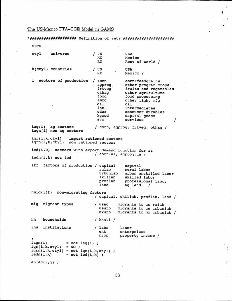
Appendix: The US-Mexico FTA-CGE Model

Introduction

This appendix presents the equations of the US-Mexico, FTA-CGE model in theformat of the software in which the program was written, GAMS. GAMS stands for"General Algebraic Modeling System" and the software is described in Brooke, Kendrick,and Meeraus (1988). For ease of exposition, the model equations are somewhat simplified.The agricultural support programs are represented by ad valorem equivalents, while thefull model specifies the programs explicitly. All sectors are shown with CET transforma-tion functions between goods supplied to the domestic and export markets. The full modelassumes that two agricultural sectors (corn and other program crops) have an infiniteelasticity of transformation between domestic and export goods. In the full model, theoutput of the oil sector in both countries is fixed exogenously.

GAMS statements are case insensitive. However, we use a number of notationconventions to improve readability:

Variables are all in upper case.Variable names with a suffix 0 represent base-year values and are specified as

parameters (or constants) in the model.Parameters are all in lower case.Sets are all in lower case.

In the GAMS language:

Parameters are treated as constants in the model and are defined in separate"PARAMETER" statements.

"SUM" represents the summation operator, sigma."PROD" represents the product operator, pi."LOG" is the natural logarithm operator."$" introduces a conditional "if' statement.The suffix .FX indicates a fixed variable.The suffix .L indicates the level or solution value of a variable.The suffix .L0 indicates the lower bound of a variable.The suffix .UP indicates the upper bound of a variables.An asterisk (*) in column one indicates a comment. Some alternative treatments

are shown commented out.A Subsets is denoted by the subset name followed by the name of the larger set in

parentheses. In statements, the subset name is then used by itself.A semicolon (;) terminates a GAMS statement.Items betweeen slashes ("/") are data.

•

37

The US-Mexico FrA—CGE Model in GAMS

*###########O######## Definition of sets ######################

SETS

ctyl universe / US USAMX MexicoRT Rest of world /

,k(ctyl) countries

i sectors of production

iag(i) ag sectorsiagn(i) non ag sectors

/ USMX

cornagprog,frtvegothagfoodlmfgoilintcdurkgoodsvc

USAMexico /

corn+feedgrainsother program cropsfruits and vegetablesother agriculturefood processingother light mfgoilintermediatesconsumer durablescapital goodsservices

/ corn, agprog, frtveg, othag /

iqr(i,k,ctyl) import rationed sectorsiqrn(i,k,ctyl) non rationed sectors

ied(i,k) sectors with export demand function for rt/ corn.us, agprog.us /

iedn(i,k) not ied

iff factors of production / capitalrulaburbunlabskillabprof labland

nmig(iff) non-migrating factors/ capital,

mig migrant types

hh households

ins institutions

iagn(i)iqr(i,k,ctyl)iqrn(i,k,ctyl)iedn(i,k)

ALIAS(i,j) ;

usagusurbmxurb

hhall

/ labrentprop

= not iaq(i) ;= NO ;= not iqr(i,k,ctyl) ;= not ied(i,k) ;

capitalrural laborurban unskilled laborskilled laborprofessional laborag land /

skillab, prof lab, land

migrants tomigrants tomigrants to

38

us rulabus urbunlabmx urbunlab

laborenterprisesproperty income /

ALIAS(k,1) ;ALIAS(ctyl,cty/) ;ALIAS(1a,lb) ;ALIAS(iff,f) ;

SET pt(k,ctyl) three trading partners / us. (mx,rt)mx. (us,rt)

/ ;

SET pt3(ctyl,cty2) two trading partners / us. (mx)mx. (us)

I;*################## Definition of variables ##################

VARIABLES

*## PRICE BLOCK

EXR(k)P(i,k)PD(i,k)PE(i,k,ctyl)PINDEX(k).PM(i,k,ctyl)PWE(i,ctyl,cty2)PWM(i,ctyl,cty2)PX(i,k)PVA(i,k)T142(i,k,ctyl)

exchange rateprice of composite gooddomestic pricedomestic price of exportsnumeraire price indexdomestic price of importsworld price of exports from ctyl-to cty2world price of imports into ctyl from cty2average output pricevalue added priceimport premium rate

*## PRODUCTION AND TRADE BLOCK

E(i,ctyl,cty2)M(i,ctyl,cty2)X(i,k)XD(i,k)XXD(i,k)SMQ(i,k,ctyl) ,INT(i,k)

*44 FACTOR BLOCK

WFDIST(i,iff,k)YFCTR(iff,k)FS(iff,k)FDSC(i,iff,k)WF(iff,k)

exports from ctyl to cty2imports into ctyl from cty2composite goods supplydomestic outputdomestic salesimport value share (AIDS function)intermediate demand

factor price distortion constantsfactor incomefactor supplyfactor demand by sectoraverage factor price

*## INCOME AND EXPENDITURE BLOCK

CDD(i,k)FSAV(k,ctyl)FBAL(k)INDTAX(k)SSTAX(k)TARIFF(k,ctyl)PREM(i,k)YH(hh,k)YINST(ins,40WALRASWALRAS2(k)

final demand for private consumptionnet foreign savingscurrent account balanceindirect tax revenuefactor taxestariff revenuepremium income from import rationinghousehold incomeinstitutional incomeWalras law for systemWalras law for each country

39

•

GDTOT(k)GD(i,k)GOVSAV(k)GOVREV(k)HHT(k)ENTT(k)ID(i,k)DST(i,k)ZTOT(k)ZFIX(k)HSAV(k)REMIT(k)FKAP(k)FBOR(k)FSAVE(k)ENTSAV(k)ESR(k)VATAX(k)ENTAX(k)HTAX(k)

EEP(i,k,ctyl)PIE(i,k)PDS(i,k)

•*## MIGRATION BLOCK

USMIGAGUSMIGURBMXMIG

government real consumptiongovernmend demand by sectorgovernment savinggovernment revenuegovt transfers to householdsgovt transfers to enterprisesinvestment demand by sector of origininventory investment demandaggregate nominal investmentaggregate real fixed investmentaggregate household savingsremittance income to householdsforeign capital flow to enterprisesforeign borrowing by governmentforeign savingsenterprise savingsenterprise savings ratevalue added taxesenterprise taxeshousehold taxes

US bilateral export subsidy expendituresproducer incentive equivalent per unit of output.domestic price subsidies per unit domestic supply

Mexican rural migrants to US rural sector• Mexican urban migrants to US urban sector

Mexican internal rural to urban migrants

*#####################

PARAMETERS

mrat(i,k,ctyl)tm(i,k,ctyl)tee(i,k,ctyl)pwts(i,k)sprem(i,k)

io(i,j,k)

rhoc(i,k)rhot(i,k)etae(i,k)ac(i,k)ad(i,k)alpha(i,iff,k)alpha2(i,iff,k)at(i,k)delta(i,k,ctyl)gamma(i,k,ctyl)

aq(i,k)aqs(i,k)smq0(i,k,cty2)

amq(i,k,ctyl)betaq(i,k,ctyl)gammaq(i,k,cty2)

Definition of Parameters ##################

rationed import leveltariff rates on importsexport subsidy (EEP) ratesprice index weightsallocation share of premium income

input output coefficients by country

CES import aggregation parameterCET export transformation parameterexport demand elasticity for rest of worldCES import function shift parameterproduction function shift parameterCobb-Douglas factor share parameterCES factor share parameterCET export function shift parameterCES import function share parameterCET export function share parameter

constant in translog price indexconstant in Stone price indexshare parameter in Stone price index

constant in aids functionincome coefficients in aids functionprice coefficients in aids function

40

•

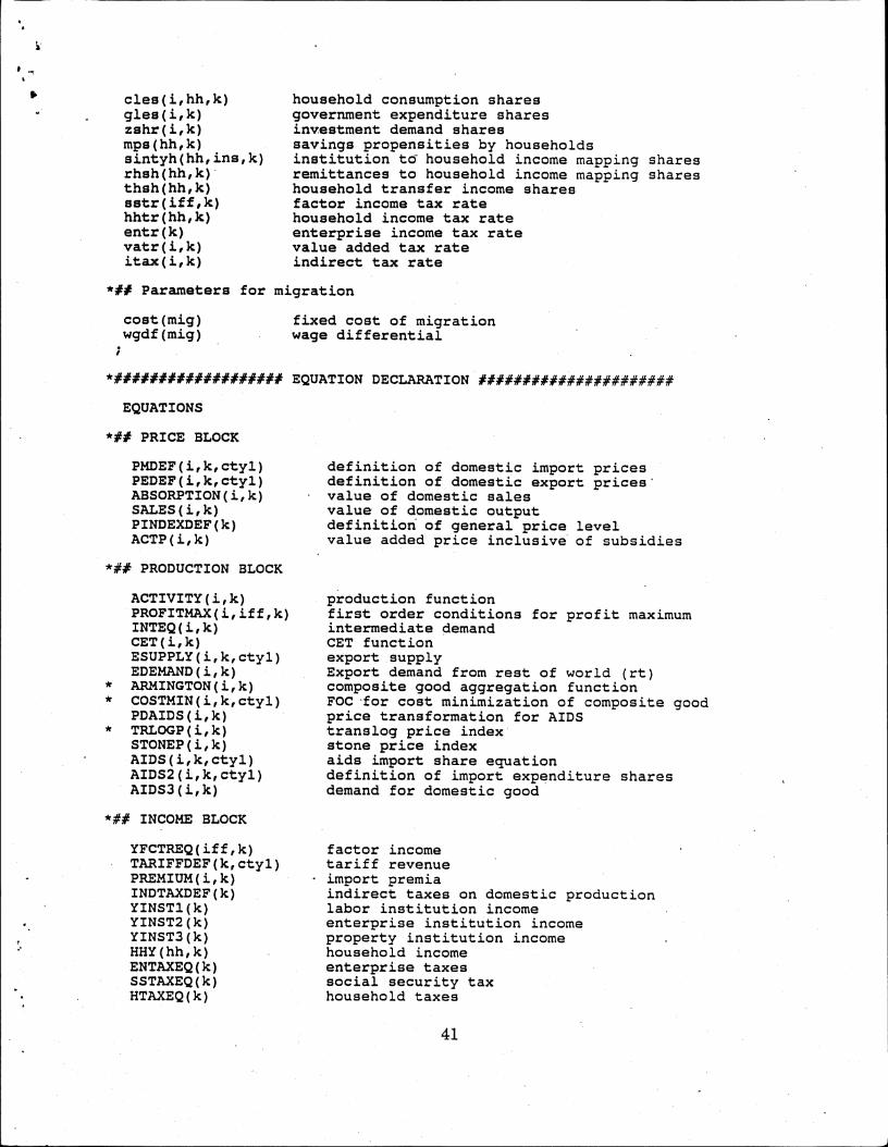
cles(i,hh,k)gles(i,k)zshr(i,k)mps(hh,k)sintyh(hh,ins,k)rhsh(hh,k)thsh(hh,k)sstr(iff,k)hhtr(hh,k)entr(k)vatr(i,k)itax(i,k)

household consumption sharesgovernment expenditure sharesinvestment demand sharessavings propensities by householdsinstitution to household income mapping sharesremittances to household income mapping shareshousehold transfer income sharesfactor income tax ratehousehold income tax rateenterprise income tax ratevalue added tax rateindirect tax rate

*## Parameters for migration

cost(mig)wgdf(mig)

fixed cost of migrationwage differential

*################### EQUATION

EQUATIONS

*## PRICE BLOCK

PMDEF(i,k,ctyl)PEDEF(i,k,ctyl)ABSORPTION(i,k)SALES(i,k)PINDEXDEF(k)ACTP(i,k)

*## PRODUCTION BLOCK

ACTIVITY(i,k)PROFITMAX(i,iff,k)INTEQ(i,k)CET(i,k)ESUPPLY(i,k,ctyl)EDEMAND(i,k)ARMINGTON(i,k)COSTMIN(i,k,ctyl)PDAIDS(i,k)TRLOGP(i,k)STONEP(i,k)AIDS(i,k,ctyl)AIDS2(i,k,ctyl)AIDS3(i,k)

*## INCOME BLOCK

YFCTREQ(iff,k)TARIFFDEF(k,ctyl)PREMIUM(i,k)INDTAXDEF(k)YINST1(k)YINST2(k)YINST3(k)HHY(hh,k)ENTAXEQ(k)SSTAXEQ(k)HTAXEQ(k)

DECLARATION ######################

definition of domestic import pricesdefinition of domestic export prices'value of domestic salesvalue of domestic outputdefinition. of general price levelvalue added price inclusive of subsidies

production functionfirst order conditions for profit maximumintermediate demandCET functionexport supplyExport demand from rest of world (rt)composite good aggregation functionFOC .for cost minimization of composite goodprice transformation for AIDStranslog price indexstone price indexaids import share equationdefinition of import expenditure sharesdemand for domestic good

factor incometariff revenueimport premiaindirect taxes on domestic productionlabor institution incomeenterprise institution incomeproperty institution incomehousehold incomeenterprise taxessocial security taxhousehold taxes

41

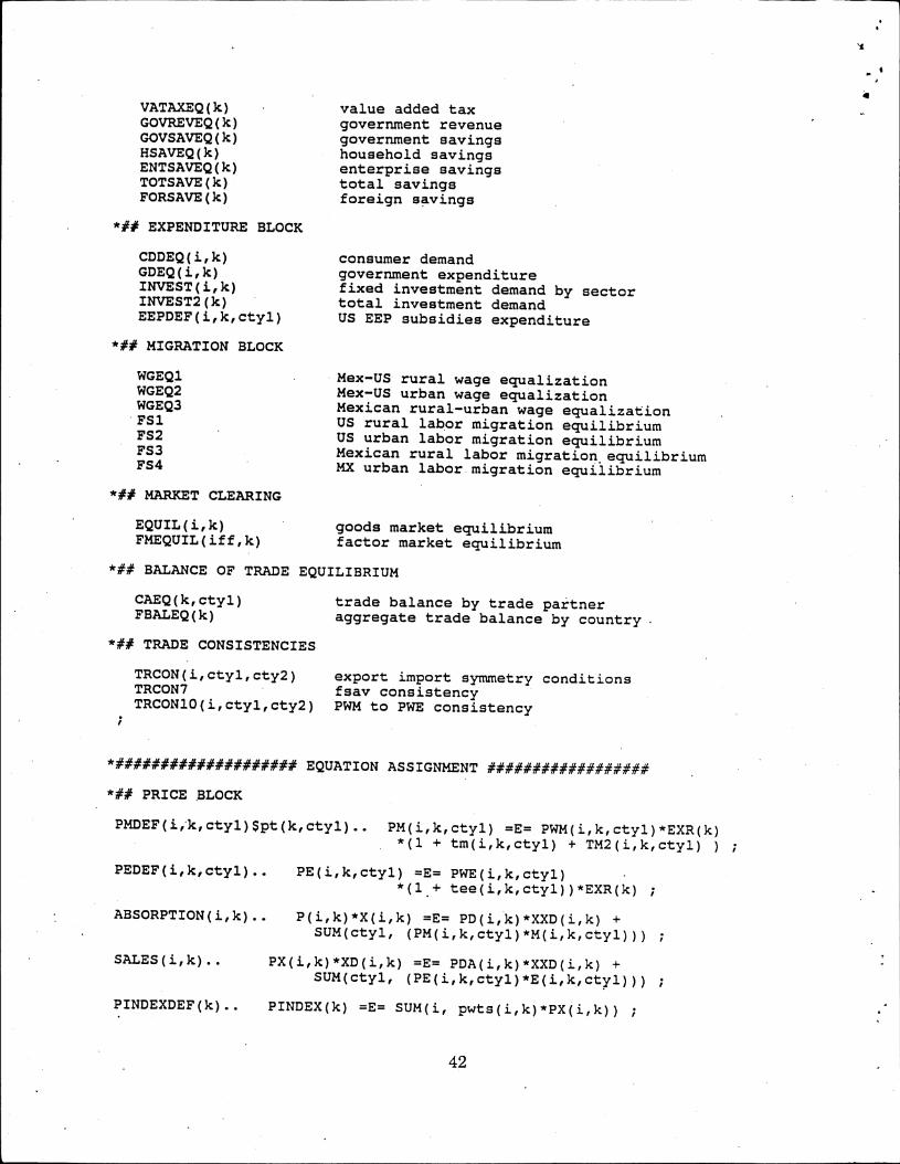
VATAXEQ(k)GOVREVEQ(k)GOVSAVEQ(k)HSAVEQ(k)ENTSAVEQ(k)TOTSAVE(k)FORSAVE(k)

*## EXPENDITURE BLOCK

CDDEQ(i,k)GDEQ(i,k)INVEST(i,k)INVEST2(k)EEPDEF(i,k,ctyl)

*## MIGRATION BLOCK

WGEQ1WGEQ2WGEQ3FS1FS2FS3FS4

*## MARKET CLEARING

EQUIL(i,k)FMEQUIL(iff,k)

value added taxgovernment revenuegovernment savingshousehold savingsenterprise savingstotal savingsforeign savings

consumer demandgovernment expenditurefixed investment demand by sectortotal investment demandUS EEP subsidies expenditure

Mex-US rural wage equalizationMex-US urban wage equalizationMexican rural-urban wage equalizationUS rural labor migration equilibriumUS urban labor migration equilibriumMexican rural labor migration equilibriumMX urban labor migration equilibrium

goods market equilibriumfactor market equilibrium

*## BALANCE OF TRADE EQUILIBRIUM

CAEQ(k,ctyl)FBALEQ(k)

*## TRADE CONSISTENCIES

TRCON(i,ctyl,cty2)TRCON7TRCON10(i,ctyl,cty2)

trade balance by trade partneraggregate trade balance by country.

export import symmetry conditionsfsav consistencyPWM to PWE consistency

*#################### EQUATION ASSIGNMENT ##################

*## PRICE BLOCK

PMDEF(i0c,cty1)$pt(k,cty1).. PM(i,k,ctyl) =E= PWM(i,k,cty1)*EXR(k)*(1 + tm(i,k,ctyl) + TM2(i,k,ctyl) )

PEDEF(i,k,cty1).. PE(i,k,ctyl) =E= PWE(i,k,ctyl)*(1.+ tee(i,k,cty1))*EXR(k) ;

ABSORPTION(i,k).. P(i,k)*X(i,k) =E= PD(i,k)*XXD(i,k) +SUM(ctyl, (PM(i,k,cty1)*M(i,k,cty1))) ;

SALES(i,k).. PX(i,k)*XD(i,k) =E= PDA(i,k)*XXD(i,k) +SUM(ctyl, (PE(i,k,cty1)*E(i,k,cty1))) ;

PINDEXDEF(k).. PINDEX(k) =E= SUM(i, pwts(i,k)*PX(i,k)) ;

42

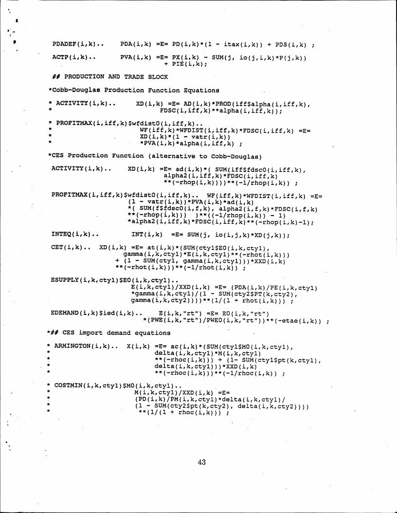
PDADEF(i,k).. PDA(i,k) =E= PD(i,k)*(1 - itax(i,k)) + PDS(i,k) ;

ACTP(i,k).. PVA(i,k) =E= PX(i,k) - SUMO, io(j,i,k)*P(j,k))+ PIE(1,k);

i# PRODUCTION AND TRADE BLOCK

*Cobb-Douglas Production Function Equations

* ACTIVITY(i,k).. XD(i,k) =E= AD(i,k)*PROD(iff$alpha(i,iff,k),FDSC(i,iff,k)**alpha(i,iff,k));

* PROFITMAX(i,iff,k)$wfdist0(i,iff,k)..WF(iff,k)*WFDIST(i,iff,k)*FDSC(i,iff,k) =E=XD(i,k)*(]. - vatr(i,k))*PVA(i,k)*alpha(i,iff,k) ;

*CES Production Function (alternative to Cobb-Douglas)

ACTIVITY(i,k).. XD(i,k) =E= ad(i,k)*( SUMUff$fdscO(i,iff,k),alpha2(i,iff,k)*FDSC(i,iff,k)li*(-rhop(i,k))))**(-1/rhop(i,k)) ;

PROFITMAX(i,iff,k)$wfdist0(i,iff,k).. WF(iff,k)*WFDIST(i,iff,k) =E=(1 - vatr(i,k))*PVA(i,k)*ad(i,k)*( SUM(f$fdsc0(i,f,k), alpha2(i,f,k)*FDSC(i,f,k)**(-rhop(i,k))) )**((-1/rhop(i,k)) - 1)*alpha2(i,iff,k)*FDSC(i,iff,k)**(-rhop(i,k)-1);

INTEQ(i,k).. INT(i,k) =E= SUM(j, io(i,j,k)*XD(j,k));

CET(i,k).• XD(i,k) =E= at(i,k)*(SUM(ctyl$E0(i,k,ctyl),gamma(i,k,cty1)*E(i,k,cty1)**(-rhot(i,k)))

+ (1 - SUM(ctyl, gamma(i,k,cty1)))*XXD(i,k)**(-rhot(i,k)))**(-1/rhot(i,k)) ;

ESUPPLY(i,k,cty1)$E0(i,k,cty1)..E(i,k,cty1)/XXD(i,k) =E= (PDA(i,k)/PE(i,k,ctyl)*gamma(i,k,cty1)/(1 - SUM(cty2$PT(k,cty2),gamma(i,k,cty2))))**(1/(1 + rhot(i,k))) ;

EDEMAND(i,k)$ied(i,k).. E(i,k,"rt") =E= E0(i,k,"rt")*(PWE(i,k,"rt")/PWE0(i,k,"rt"))**(-etae(i,k))

*## CES import demand equations

* ARMINGTON(i,k).. X(i,k) =E= ac(i,k)*(SUM(ctyl$M0(i,k,ctyl),delta(i,k,cty1)*M(i,k,ctyl)**(-rhoc(i,k))) + (1- SUM(ctyl$pt(k,ctyl),delta(i,k,ctyl.)))*XXD(i,k)**(-rhoc(i,k)))**(-1/rhoc(i,k)) ;

* COSTMIN(i,k,cty1)$M0(i,k,cty1)..M(i,k,cty1)/XXD(i,k) =E=(PD(i,k)/PM(i,k,cty1)*delta(i,k,cty1)/(1 - SUM(cty2$pt(k,cty2), delta(i,k,cty2))))**(1/(1 + rhoc(i,k))) ;

43

*## AIDS import demand equations. Alternative to CES version. In AIDS*## version, can use Stone or translog price index. Notation*## is that domestically produced goods sold on the domestic*## market are indicated as imports from a country to itself.

PDAIDS(i,k).. PM(1,k,k) =E= PD(i,k) ;

*##.Translog price index* TRLOGP(i,k).. LOG(P(i,k)) =E= aq(i,k) + SUM(cty2, amq(i,k,cty2)

*LOG(PM(i,k,cty2))) + (1/2)*SUM((ctyl,cty2),gammaq(i,k,ctyl,cty2)*LOG(PM(i,k,cty1))*LOG(PM(i,k,cty2))) ;

*## Stone price indexSTONEP(i,k).. LOG(P(i,k)) =E= LOG(aqs(i,k)) + SUM(cty2,

SMQ0(i,k,cty2)*LOG(PM(i,k,cty2))) ;

AIDS(i,k,cty1).. SMQ(i,k,ctyl) =E= amq(i,k,ctyl) + betaq(i,k,ctyl)*LOG(X(i,k)) + SUM(cty2, gammaq(i,k,ctyl,cty2)*LOG(PM(i,k,cty2))) ;

AIDS2(i,k,cty1)$pt(k,cty1)..PM(i,k,cty1)*M(i,k,ctyl) =E=

SMQ(i,k,cty1)*P(i,k)*X(i,k) ;

AIDS3(i,k)..

*## INCOME BLOCK

YFCTREQ(iff,k)..

TARIFFDEF(k,ctyl)

PREMIUM(i,k)..

INDTAXDEF(k)..

YINST1(k)..

YINST2(k)..

YINST3(k)..

HHY(hh,k)..

ENTAXEQ(k)..

SSTAXEQ(k)..

HTAXEQ(k)..

. PD(i,k)*XXD(i,k) =E= SMQ(i,k,k)*X(i,k)*Pli,k) ;

YFCTR(iff,k) =E= SUM(i, WF(iff,k)*WFDIST(i,iff,k)*FDSC(i,iff,k));

• • TARIFF(k,ctyl) =E= SUM(i, tm(i,k,ctyl)*M(i,k,cty1)*PWM(1,k,ctyl))*EXR(k) ;

PREM(i,k) =E= SUM(ctyl, TM2(i,k,cty1)*M(i,k,ctyl)*PW4(i,k,cty1))*EXR(k) ;

INDTAX(k) =E= SUM(i, itax(i,k)*PD(i,k)*XXD(i,k)) ;

YINST("labr",k) =E= SUM(la, (1.0 - sstr(la,k))*YFCTR(la,k));

YINST("ent",k) =E= YFCTR("capital",k)*(1.0-sstr("capital",k))+ EXR(k)*FKAP(k) - ENTSAV(k)- ENTAX(k) + ENTT(k) -+ SUM(i, (1-sprem(i,k))*PREM(i,k))

YINST("prop",k) =E= YFCTR("land",k)*(1.O_ sstr("land",k)) ;

YH(hh,k). =E= SUM(ins, sintyh(hh,ins,k)*YINST(ins,k))+ rhsh(hh,k)*EXR(k)*REMIT(k)+ HHT(k)*thsh(hh,k) ;

ENTAX(k)

SSTAX(k)

HTAX(k)

=E= ENTR(k)*(YFCTR("capital",k) + ENTT(k)) ;

=E= SUM(iff, sstr(iff,k)*YFCTR(iff,k));

=E= SUM(hh, hhtr(hh,k)*YH(hh,k)) ;

44

VATAXEQ(k).. VATAX(k)

GOVREVEQ(k).. GOVREV(k)

GOVSAVEQ(k).. GOVSAV(k)

HSAVEQ(k).. HSAV(k)

ENTSAVEQ(k).. ENTSAV(k)

TOTSAVE(k).. ZTOT(k)

FORSAVE(k).. FSAVE(k)

*I# EXPENDITURE BLOCK

CDDEQ(i,k)..

=E= SUM(i, vatr(i,k)*PVA(i,k)*XD(i,k)) ;

=E=

=E=

SUM(ctyl, TARIFF(k,cty1)) + INDTAX(k)SUM(i, sprem(i,k)*PREM(i,k))SSTAX(k) + HTAX(k)ENTAX(k) + VATAX(k) + FBOR(k)*EXR(k);

GOVREV(k)SUM(i, GD(i,k)*P(i,k)) - HHT(k)ENTT(k) - FPE(k)SUM((j,ctyl) EEP(j,k,cty1)) ;

=E= SUM(hh,.mps(hh,k)*((1.0-hhtr(hh,k))*YH(hh,k)));

=E= ESR(k)*YFCTR("capital",k) ;

=E= GOVSAV(k) + HSAV(k)+ ENTSAV(k) + EXR(k)*FSAVE(k);

=E= FBAL(k)-FKAP(k)-FBOR(k)-REMIT(k);

P(i,k)*CDD(i,k) =E= SUM(hh, cles(i,hh,k)*YH(hh,k)*(1 - hhtr(hh,k))*(1 mps(hh,k)));

GDEQ(i,k).. GD(i,k) =E= g.les(i,k)*GDTOT(k) ;

INVEST(i,k).. ID(i,k) =E= zshr(i,k)*ZFIX(k) ;

INVEST2(k).. ZTOT(k) =E= SUM(i, P(i,k)*(ID(i,k) + DST(i,k)).)+ WALRAS2(k) ;

EEPDEF(i,k,cty1).. EEP(i,k,ctyl) =E= tee(i,k,cty1)*PWE(i,k,ctyl)*t(i,k,cty1)*EXR(k) ;

*## MARKET CLEARING*## PRODUCT MARKETS

EQUIL(i,k).. X(i,k) =E= INT(i,k)+CDD(i,k)+GD(i,k)+ID(i,k)+DST(i,k);

*44 FACTOR MARKETS

FMEQUIL(iff,k)..

WGEQ1..

WGEQ2..

WGEQ3..

FS1..

SUM(i, FDSC(i,iff,k)) =E= F§(iff,k) ;

WF("rulab","mx")=E=(wgdf( "usag")*WF("rulab","us")- COST("usag"))*(EXR("mx")/EXR("us")) ;

WF("urbunlab","mx")=E=(wgdf("usurb")*WF("urbunlab","us")- COST("usurb"))*(EXR("mx")/EXR("us")) ;

WF("rulab","mx")=E=(wgdf("mxurb")*WF("urbunlab","mx"- COST("mxurb")) ;

FS("rulab","us")

FS2.. FS("urbunlab","us")

FS3.. FS("rulab","mx")

FS4.. FS("urbunlab","mx"

FSO("rulab","us") + USMIGAG ;

=E= FSO( "urbunlab","us") + USMIGURB

=E= FSO("rulab","mx") - MXMIG - USMIGAG ;

=E= FS0("urbunlab","mx") + MXMIG

45

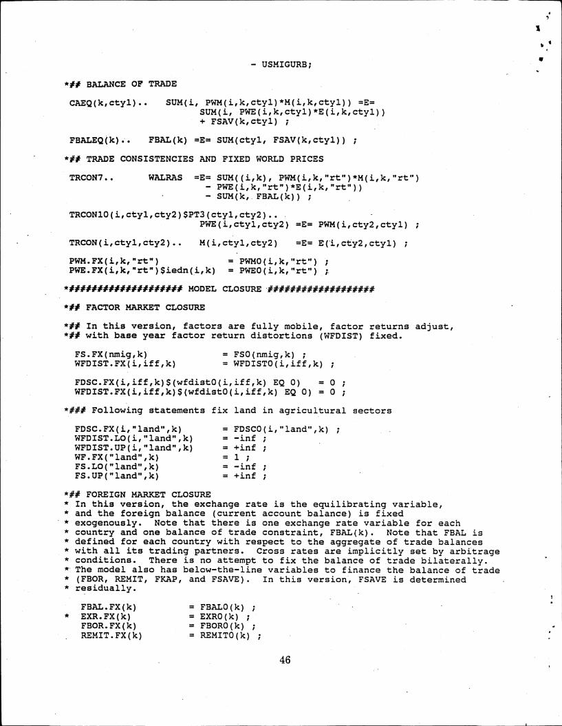
- USMIGURB;

44# BALANCE OF TRADE

CAEQ(k,cty1).. SUM(i, PWM(i,k,cty1)*M(i,k,cty1)) =E=SUM(i, PWE(i,k,cty1)*E(i,k,cty1))+ FSAV(k,ctyl) ;

FBALEQ(k):. FBAL(k) =E= SUM(ctyl, FSAV(k,cty1)) ;

*## TRADE CONSISTENCIES AND FIXED WORLD PRICES

TRCON7.. WALRAS =E= SUM((i,k), PWM(i,k,"rt")*M(i,k,"rt")- PWE(i,k,"rt")*E(i,k,"rt"))- SUM(k,.FBAL(k)) ;

TRCON10(i,ctyl,cty2)$PT3(ctyl,cty2)..PWE(i,ctyl,cty2) =E= PWM(i,cty2,ctyl)

TRCON(i,ctyl,cty2).. M(i,ctyl,cty2) =E= E(i,cty2,cty1) ;

PWM.FX(i,k,"rt") = PWM0(i,k,"rt")PWE.FX(i,k,"rt")$iedn(i,k) = PWE0(i,k,"rt")

*#################### MODEL CLOSURE ###################

*## FACTOR MARKET CLOSURE

*## In this version, factors are fully mobile, factor returns adjust,*## with base year factor return distortions (WFDIST) fixed.

FS.FX(nmig,k) = FS0(nmig,k) ;WFDIST.FX(i,iff,k) = WFDISTO(i,iff,k) ;

FDSC.FX(i,iff,k)$(wfdist0(i,iff,k) EQ 0) = 0 ;WFDIST.FX(i,iff,k)$(wfdist0(i,iff,k) EQ 0) = 0 ;

*### Following statements fix land in agricultural sectors

FDSC.FX(i,"land",k)WFDIST.L0(i,"land",k)WFDIST.UP(i,"land",k)WF.FX("land",k)FS.LO("land",k)FS.UP("land",k)

= FDSCO(i,"land",k) ;= -inf ;= +inf ;= 1 ;= -inf ;= +inf ;

*## FOREIGN MARKET CLOSURE* In this version, the exchange rate is the equilibrating variable,* and the foreign balance (current account balance) is fixed* exogenously. Note that there is one exchange rate variable for each* country and one balance of trade constraint, FBAL(k). Note that FBAL is* defined for each country with respect to the aggregate of trade balances* with all its trading partners. Cross rates are implicitly set by arbitrage* conditions. There is no attempt to fix the balance of trade bilaterally.* The model also has below-the-line variables to finance the balance of trade* (FBOR, REMIT, FKAP, and FSAVE). In this version, FSAVE is determined* residually.

FBAL.FX(k)* EXR.FX(k)

FBOR.FX(k). REMIT.FX(k)

= FBALO(k) ;= EXR0(k) ;= FBORO(k) ;= REMITO(k) ;

46

4,

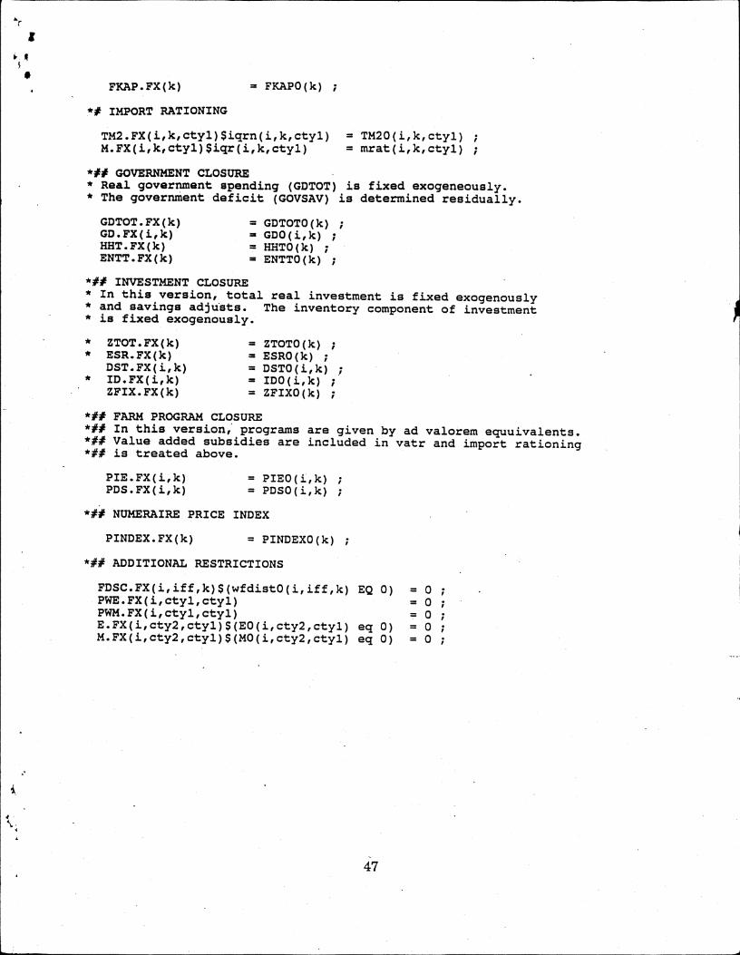
• FKAP.FX(k)

*# IMPORT RATIONING

= FKAPO(k) ;

TM2.FX(i,k,ctyl)Siqrn(i,k,ctyl) = TM20(i,k,ctyl) ;M.FX(i,k,cty1)$iqr(i,k,ctyl) = mrat(i,k,ctyl) ;

*## GOVERNMENT CLOSURE* Real government spending (GDTOT) is fixed exogeneously.* The government deficit (GOVSAV) is determined residually.

GDTOT.FX(k)GD.FX(i,k)HHT.FX(k)ENTT.FX(k)

= GDTOTO(k) ;= GDO(i,k) ;= HHT0(k) ;= ENTTO(k) ;

*## INVESTMENT CLOSURE* In this version, total real investment is fixed exogenously* and savings adjusts. The inventory component of investment* is fixed exogenously.

• ZTOT.FX(k) = ZTOTO(k) ;• ESR.FX(k) = ESRO(k) ;

DST.FX(i,k) = DSTO(i,k) ;• ID.FX(i,k) = IDO(i,k) ;

ZFIX.FX(k) = ZFIXO(k) ;

*## FARM PROGRAM CLOSURE*## In this version, programs are given by ad valorem equuivalents.*## Value added subsidies are included in vatr and import rationing*## is treated above.

PIE.FX(i,k) = PIE0(i,k) ;PDS.FX(i,k) = PDS0(i,k) ;

• NUMERAIRE PRICE INDEX

PINDEX.FX(k) = PINDEX0(k) ;

*## ADDITIONAL RESTRICTIONS

FDSC.FX(i,iff,k)$(wfdist0(i,iff,k) EQ 0) = 0 ;PWE.FX(i,ctyl,ctyl) = 0 ;PWM.FX(i,ctyl,ctyl) = 0 ;E.FX(i,cty2,ctyl)$(E0(i,cty2,ctyl) eq 0) = 0 ;M.FX(i,cty2,cty1)$(M0(i,cty2,ctyl) eq 0) = 0 ;

47