Agricultural Risk and Remittances:

The Case of Uganda

Stefanija Veljanoska∗

Abstract

The economic literature showed that remittances could replace missing credit and insurance

markets. As a result, it is natural to expect that higher amounts of remittances will motivate

agricultural farmers to engage in riskier activities. The present study aims to verify the latter

hypothesis by answering two distinct questions: do households that receive higher remittances

choose to cultivate a riskier crop portfolio; do households that receive higher remittances choose

to engage either in crop specialization or in crop diversification? I use the Living Standards

Measurement Study-Integrated Surveys on Agriculture (LSMS-ISA) dataset on Uganda established

by the World Bank to test these hypotheses. The results show that remittances have no significant

impact on farmers’ risk decisions in terms of crop portfolio and crop diversification. There is some

evidence that credit constrained households that receive remittances engage in crop specialisation,

which can be interpreted as a wealth effect.

JEL Classification: O13, O15, Q12

Keywords: agricultural risk, crop diversity, insurance, remittances, Uganda

∗Paris School of Economics, C.E.S. - Université de Paris 1 Panthéon-Sorbonne; 106-112, Boulevard de l’Hôpital, 75647Paris Cedex 13, France. Email: veljanoska.stefanija@gmail.com

1

1 Introduction

The stock of migrants in the world is 215.8 million people which represents about 3.2 percent

of the total world population [World Bank, 2010]. The major part of these migrants comes from

the developing world: 171.6 million international and local migrants [World Bank, 2013]. This trend

is followed by an important increase in the amount of remittances sent to the developing countries

which achieved a level of $401 billion in 2012 and provide a financial flow that is higher than the

official development aid [World Bank, 2010]. It is expected that remittances in developing countries

will grow even faster. Today the growth rate of remittances in developing countries is 5.3 percent and

is expected to reach 8.8 percent during 2013-15. This phenomenon confirms the "New economics of

labour migration" (NELM) assumption that the decision of a household member to migrate is taken

collectively by the household and migrants keep interacting economically with their remaining family

[Stark, 1991]. Given the size of these financial transfers, it is essential to study their effect on remaining

households’ decision making. Taking into account that the agricultural sector represents 17 percent

of the African GDP and that 75 percent of the African population live in rural areas, investigating

the impact of remittances on different agricultural outcomes and agricultural behaviour is crucial for

understanding farm organization.

The NELM assumes that migration and remittances have the role to replace missing credit and

insurance markets by generating informal risk-sharing strategies. The mechanism behind this hypoth-

esis is the following: consider a household which sends a migrant away from his home such that the

covariance of facing a negative shock of the remaining household and the migrant simultaneously is

zero and thus diversifies the sources of income for both parts [Stark and Levhari, 1982]. In this sense,

migration is considered to be an insurance strategy, as remittances will serve to absorb any negative

shock of the remaining household and to smooth consumption. Yang and Choi [2007] and Gubert

[2002] showed that households facing a negative crop income shock received higher amounts of remit-

tances, but the received amount did not allow them to fully buffer the shock. Notwithstanding, it is

intuitive to expect that better insured households (households with higher remittances) are those that

will undertake riskier agricultural activities and will have less need to diversify their production. By

riskier agricultural activity, I include the crop choice of the farmer in terms of risk and secialisation or

diversification choices.

The first question that the present study seeks to answer is whether households that receive re-

mittances increase the riskiness of their crop production by cultivating more crops with higher but

uncertain revenue. Damon [2010] studies this question by estimating how basic grains acreage, coffee

acreage and other cash crop acreage respond to remittances. She finds that this hypothesis is not

2

supported by data from agricultural households in El Salvador as the land area dedicated to basic

grains increases and the area dedicated to commercial cash crops decreases with remittances and mi-

gration. In an analysis on community-level data Gonzalez-Velosa [2011] finds that remittances reduce

the proportion of farmers cultivating low income crops (corn, coconut) and increase the proportion

of farmers cultivating high income crops (mango). Thus these two studies do not show a consensus.

Instead of focusing only on a selected types of crops, the novelty of the present study is to construct a

measure of riskiness of each crop cultivated by a given household and to evaluate how different crops

contribute to the riskiness of the total crop portfolio by taking into account the interdependence that

might exist at a farm level and afterwards to study its relation to remittances. In that way the research

question can be reformulated as: does the riskiness of the crop portfolio of a household increase with

remittances? To this end, I will use the Single Index Model (SIM) developed by Turvey [1991] and

applied by Bezabih and Di Falco [2012] in order to construct the measure of the individual crop and

portfolio riskiness.

Following the intuition that migration and remittances represent an alternative for missing credit

and insurance markets, a second question arises: do households with higher amounts of remittances

engage in crop specialisation or crop diversification? There are two possible answers. On the one hand,

farmers that receive higher remittances might choose more specialized crop production as specialization

is seen as a risk increasing strategy. In addition, as their income is spatially diversified, then there is less

need to use crop diversification as an ex ante insurance. Gonzalez-Velosa [2011] shows that remittances

increase the probability of specialization (by reducing the number of cultivated crops) in either high-

risk crops or low-risk crops. Another possible mechanism is that as remittances increase household’s

wealth and households with higher wealth can deal more easily with risk, remittances induce crop

specialisation as a consequence of this wealth effect. On the other hand, several studies showed that

farmers in developing countries under-diversify their portfolio due to knowledge and financial barriers

[Di Falco et al., 2007, Di Falco and Chavas, 2009] . In particular, remittances are seen as substitutes or

complements to rural loans [Richter, 2008]. In other words, they can relax credit constraints directly by

substituting them and indirectly by initiating a risk adverse household to take a loan that previously

was not taken because of fear of losing the collateral. Therefore, it is possible that farmers can diversify

more their crop production with the help of remittances. This paper seeks to answer this question

by complementing the existing literature with other measures of diversification such as the Shannon

index, the Simpson index and the Berger-Parker index which take into account the distribution of

shares to each variety and not only the number of different crops [Baumgärtner, 2004].

In order to test for the impact of remittances on the agricultural outcomes discussed before (pro-

duction riskiness and degree of crop diversification), I will use an Instrumental Variable approach

(IV). Estimating this impact by Ordinary Least Squares (OLS) will yield biased results. The diversity

3

indices (Inverse Simpson, Shannon and Berger-Parker index) are left-censored which requires a Tobit

estimation model. Also, remittances are not random and depend on household characteristics. Thus,

households that have migrants and receive remittances may differ from those households that have

neither migrants nor remittances, which might be based on some unobservable characteristics of the

household. At the same time, there might be some household unobservable characteristics that have

a simultaneous impact on migration, remittances and agricultural decisions such as entrepreneurial

spirit. I solve this issue by using an instrumental variable (IV) approach and using district level of

migrants as instruments. The results show that remittances have no significant impact on farmers’

risk decisions in terms of crop portfolio and crop diversification. However, there is some evidence

that credit constrained households that receive remittances engage in crop specialisation, which can

be interpreted as a wealth effect.

The answers to these questions have important policy implications. On the one hand, the economic

literature state that African farmers choose low yield/low risk portfolios because of their negative past

experience (weather shocks). This is mostly due to missing insurance and credit markets, but also

absence of irrigation systems. It was shown that low yield portfolios are suboptimal, and taking more

risk in the decision making can increase the efficiency of the household agricultural portfolio as farmers

forgo more profitable opportunities for the sake of certainty [Mendola, 2008]. Farmers in developing

countries choose low-risk portfolios and low-risk production technologies that result in low yields in

order to avoid the damages of weather shocks that occur often. Therefore, the existence of insured

risk makes households stuck in poverty traps, especially when households are obliged to avoid risk as

this risk is linked to their subsistence needs. The consequences are amplified in the case of African

farms when considering climate change. The African continent is the most vulnerable to climate

change. Adaptation to climate change by cropping drought/flood resistant crops will make a pressure

on farmers to engage in risk avoidance thus pushing them into poverty.

2 The Context

Uganda is a landlocked country situated in East Africa with about 34 million inhabitants. The

Ugandan agricultural sector represents about 23 percent of its GDP a share that has declined in the

last years [World Bank, 2011]. Still, the agricultural sector employs about 71 percent of the active

population and covers about 70 percent (around 17 million ha) of the total area that is available for

cultivation [FAOSTAT, 2011]. This confirms the importance of Ugandan agriculture for the country’s

economy. Ugandan agriculture is mostly rain-fed and it benefits from the number of lakes and rivers

present in the country. Uganda’s climate is tropical, generally rainy (particularly during the months of

March to May and September to November), while the remaining months, from December to February

4

and from June to August represent Uganda’s two dry seasons.

2.1 The sample

I use data from the Living Standards Measurement Study-Integrated Surveys on Agriculture

(LSMS-ISA) established by the Bill and Melinda Gates Foundation and implemented by the Living

Standards Measurement Study (LSMS) within the Development Research Group at the World Bank.

The Uganda National Panel Survey (UNPS) sample includes economic and social information on about

3.200 households (with about 2000 households that are engaged in agriculture). These households were

previously interviewed in the 2005/2006 Uganda National Household Survey (UNHS). The sample also

includes households that were randomly selected after 2005/2006. This sample is representative at the

national, urban/rural and main regional levels (North, East, West and Central regions). Afterwards,

the initial sample was visited for two consecutive years (2009/10 and 2010/11).

2.2 The descriptive statistics

The surveys on the agricultural activities in the LSMS-ISA include information on the two separate

cropping seasons: from January to June and from July to December. Interviewing households twice a

year allows to reduce the recall bias that is due to poor household accountability. In order to better

understand the crop choice patterns of the sample, I calculated the share of households cultivating a

given crop (Table 1) and the average contribution of each crop to the total value of each household’s

production (Table 2). According to Table 1, the major cereal crops are maize, cassava, finger millet

and sorghum; important vegetables and fruits are beans, groundnuts, sweet potatoes and food banana;

the traditional cash crops are coffee and to some extent cotton and sugarcane. What we observe is

that, on average, other crops than cash crops are (mostly) included in the household’s portfolio even if

their average contribution to the average production value is lower than that of cash crops. On the one

hand, the average revenue coming from each of these (other than cash) crops constitutes less than one

fourth of the total average agricultural revenue. On the other hand, households that cultivate a cash

crop have a return from this cultivation that is more than a third of the total revenue. For example,

about 75.2 percent of the households cultivated maize in the first wave of the survey (2005/2006) and

the revenue coming from maize on average represents only 22.6 percent of the total. There is also

about 1.8 percent of the households that cultivate tobacco, the revenue of which accounts for 39.3

percent of the average total household production income.

Given these average statistics on the crop choices in the sample, I proceed with construction of the

different types of dependent variables based on what households crop, how they allocate inputs (land)

and the kind of production technologies they use. Three different sets of dependent variables will be

5

Table 1: Share of Households cultivating:Crop: 2005-2006 2009-2010 2010-2011

wheat 0.26 0.23 0.05barley 0.04 / /millet 25.6 24.4 21.3rice 4.8 4.5 5maize 75.2 73.4 71.3sorghum 28.2 28.7 22beans 67 71.9 70field peas 2.8 6.4 6pigeon peas 4.6 5.8 4chick peas 0.57 0.05 /cow peas 4.3 1.7 1.5ground nuts 30.5 33 32soya beans 3.6 5.3 6.8sunflower 2.9 3.4 5simsim 9.5 11.7 10cabbage 1.4 1.7 2tomatoes 3.3 3.9 3.8carrots 0.04 / 0.1onions 1.1 1.2 1.3pumpkins 1.5 2.2 3dodo 0.5 0.9 1eggplants 0.8 1.5 1sugarcane 3.7 4.5 3.8tobacco 1.8 2.3 1.6Irish potatoes 6.9 6.2 6sweet potatoes 54.1 58.4 58cassava 62.4 68.8 71yam 6 4.9 6.4oranges 0.8 1.2 1.5paw paw 2 0.8 1.5pineapples 3.1 1.4 1.4banana food 47.5 46.7 50banana beer 16.2 8.7 11.2banana sweet 10.4 6.2 7.8mango 1.7 1.2 2Jack fruit 3.2 1.5 3avocado 3 1.9 3passion fruit 1.2 0.5 0.6coffee 27.6 25.3 27.5cotton 9.4 2.5 4.2cocoa 0.8 0.8 0.6tea 0.3 0.19 0.2vanilla 2.8 0.7 0.4N 2282 2130 1979

6

Table 2: Average Crop Revenue ShareCrop: 2005-2006 2009-2010 2010-2011

wheat 6.8 2.5 0barley / / /millet 13.8 12.75 16.35rice 27 26.6 32.2maize 22.6 25 19.7sorghum 19.7 13.4 18beans 17.5 19.7 22field peas 11.5 18 14.35cow peas 7.4 6.7pigeon peas 7.8 8.3 6.5chick peas 8.9 9.3 5.6ground nuts 18.15 13.5 17.5soya beans 9.3 11 7.9sunflower 15 16 22.7simsim 17.3 18 22.9cabbage 11.5 8.45 15.8tomatoes 15.9 18.5 14,77carrots 2.25 / 1.2onions 18.4 9.45 7pumpkins 6.3 10.2 3.4dodo 3.7 11.4 12.8eggplants 5.1 3.7 4.6sugarcane 14.5 19 15.4tobacco 39.3 39.4 40.2Irish potatoes 13.8 13.5 11sweet potatoes 20.2 16.4 15cassava 19.5 15.8 17,6yam 6.6 9 6.6oranges 4.5 8 6.25paw paw 3.2 9 6pineapples 6.7 11.8 9.2banana food 30.7 32.9 34banana beer 7.4 11 7banana sweet 4.1 5 5mango 2.8 3.8 9Jack fruit 5.6 5.3 4avocado 2.9 11.7 3.3passion fruit 13.8 14.8 21coffee 17 16.8 17cotton 19.8 22.7 26.5cocoa 32.1 41 48tea 21.8 21.7 40ginger 0 26.9 0vanilla 3.2 3 14.2N 2282 2130 1979

7

used in the analysis. The first dependent variable is the weighted portfolio beta which is an average

of each beta from a Single Index Model estimation for the crops cultivated by a given household. The

construction of this variable is explained in detail in Section 3. The second set of dependent variables is

constituted of different diversity indices that are borrowed from the ecological literature [Baumgärtner,

2004]. I limit my study to the interspecific aspect of diversity, including the diversity measures the

different crops, but not the different varieties of a given crop. The diversity indices can be classified

into three groups. The first category refers to the simplest measure of biodiversity named as richness

index and it represents the total number of different species in the ecosystem. In the present study, this

richness index represent the total number of crops cultivated by a household on its land. The richness

index assumes an equal contribution of each crop to the household’s crop diversity. However, one might

argue that different crops should account differently for the degree of diversity. As a reaction, indices

of absolute or relative abundance were developed in the literature. The second category of diversity

index takes into account the dominance of certain species/crops over other. In particular, the Berger-

Parger index (BP) takes into account the inverse weight of most abundant species/crop. According

to this definition, the lower the share of the land dedicated to the most abundant crop, the higher of

the value of the BP. The third group of diversity, Simpson index and Shanon index indices, include

in their definition the richness and the evenness of crops. The evenness refers to level of equality of

the abundance of different species/crops. Following to this, a higher value of these indices is due to a

higher number of species but also a higher equality of the abundance of the different species. In the

present study, the latter can be interpreted as equal land shares among different crops.

Tables 3, 4 and 5 describe the summary statistics of the dependent variables. I will comment on

the statistics of the weighted portfolio beta once the construction of this variable is explained. The

statistics on the richness measure shows that on average, households planted 4.92 crops in the period

from 2009 to 2011. The average number of cultivated crops increased between the two periods from

4.77 to 5.1 (Table 4 and 5). Eighty percent of the households cultivated two to six crops and only

three percent of the households cultivated only one crop with the median being five crops during the

whole period. What can be noted is that other diversity variables are lower than the count index which

indicates that land is not equally distributed to different crops. All the three indices are left-censored

for households that cultivate one crop and their mean value increases from one year to the other. This

increase can be due to the increase of the number of cultivated crops, but also from a more equal

allocation among different crops.

Table 6 presents definitions and the summary statistics of the explanatory variables and the other

control variables that will be used in the estimations. The main variable of interest is the level of re-

mittances that a household receives from migrants. As discussed above, it is expected that remittances

have a positive impact on the riskiness of crop portfolio but the impact on crop diversification is less

8

Table 3: Summary statistics: Dependent variableStandard

Variable name Mean Deviation Min. Max.

Risk variableweighted portfoliobeta .285 .491 0 7.604

Interspecific diversity variablescount index n 4.916 2.068 1 16inverse Simpson 3.302 1.358 1 9.404Shannon 1.258 0.446 0 2.304Berger-Parker 2.372 0.875 1 6.792

Table 4: Summary statistics: Dependent variable wave 2009-2010Standard

Variable name Mean Deviation Min. Max.

Risk variableweighted portfolio beta 0.291 0.539 0 7.605

Interspecific diversity variablescount index n 4.775 2.069 1 13inverse Simpson 3.196 1.328 1 8.082Shannon 1.22 0.454 0 2.269Berger-Parker 2.313 0.849 1 6

Table 5: Summary statistics: Dependent variable wave 2010-2011Standard

Variable name Mean Deviation Min. Max.

Risk variableweighted portfolio beta 0.278 0.447 0 6.085

Interspecific diversity variablescount index n 5.067 2.056 1 16inverse Simpson 3.415 1.381 1 9.404Shannon 1.299 0.435 0 2.304Berger-Parker 2.435 0.899 1 6.792

9

evident. About thirty five percent of the households in the dataset reported to receive remittances

locally or from abroad. The mean value of remittances is 107 363 Shs per household. About twenty two

percent of the households have a migrant, a person that left the household for more then six months or

left it permanently. The mean level of migrants is 0.38 per household. Among the households having

migrants, on average there are 1.46 migrants per household.

Table 6: Summary statistics: Explanatory variablesVariable Mean

Migration and Remittances

migrants migrants of the hh, locally or abroad t-1 .38

remittances received by the hh from migrants 107 3631

locally or abroad in t-1 (Shs)ditlevelmig mean district level of migrants t-1 .58

ditlevelremit mean district level of remittances t-1 (Shs) 114 6652

Household characteristics

sex the gender of the hh head 0.711equals 1 if the hh head is male

age the age of the hh head 46.95

education the highest school level achieved by the hh head 1.1111-primary, 2-secondary, 3-post secondary training, 4-higher studies

adults hh member between 16 and 65 years 2.85

dep. ratio the dependancy ratio of the hh 1.73

Wealth characteristics

non agricultural income income coming from non agricultural activities (Shs) 703 2233

assets total assets in monetary value (Shs) 5 855 4514

constraint credit/liquidity constraint dummy 0.496equals 1 if the household is constrained, 0 otherwise

Land characteristics

land agricultural land ownings in hectars 3.18

topography Number of plots with different slope 1.241

soiltexture Number of plots with different texture 1.1

soilquality Number of plots with different quality 1.092

qualityindex weighted index of soil quality 1.439with: level 1 being good quality and level 3 being poor quality

Controlling for socio-economic factors such as sex, age and education of the household’s head is1corresponds to 31.88 euros2corresponds to 34.05 euros3corresponds to 208.80 euros4corresponds to 1738.60 euros

10

important as several studies showed that household heads with different gender, age and education

level have different risk choices. It has been shown that older and female household heads choose lower

risk activities [Bezabih and Di Falco, 2012]. Household heads with higher education may choose low

risk activities as they might have more information on the negative consequences of taking risk. Also,

the number of adults of the household and the land owning are included as they are the principle

production factors and thus can impact the crop production decision making. The dependency ratio

can also be a factor that influences the risk behaviour of households as the number of non working

members can be a barrier to risk. Higher land owning might increase the possibility of diversification.

Also, riskier crops can be labour intensive, thus labour will have a positive impact on the riskiness of

the crop portfolio and eventually crop divesification.

Another important factor that concerns the risk taking of the household is its wealth. It is well

known in the economic literature that richer households can smooth more easily their consumption

when facing a negative shock than poorer households. Land owning and other assets (jewellery, houses,

radio etc) are used to control for the effect that different levels of wealth can have on the risk behaviour

of households. A variable that defines a dummy whether a household is credit/ liquidity constrained is

included too. Such a constraint can be overcome by remittances, but also by another form of income

diversification such as off-farm activities that is represented by a non-agricultural income. However, the

covariance between the agricultural and non-agricultural income in the same location should be higher

than the covariance of agricultural income and remittances from different places, thus remittances

should offer higher insurance than non-agricultural income earned in the same location.

The previously described control variables are included when examining the impact of remittances

on risk and diversification decisions and fertilizer use. In addition, the number of plots with different

slope, quality and texture are included as a higher number of different plots might facilitate the

diversification [Cavatassi et al., 2012]. A weighted index of land quality is included too in order to

capture the fact that cultivating riskier crops might demand a higher quality of land. The land quality

is measured by three different categories: 1 if good quality, 2 if medium quality and 3 if poor quality.

These categories are multiplied by the weight of each parcel in the total cultivated land and then the

weighted sum represents the quality index.

Household heads have on average 46.95 years, are mostly male (about seventy percent) and have

on average attended only primary school. Only two percent of the households did not receive any

education. The average number of adult members of the households is 2.85 and the average dependency

ratio is 1.73, which means that for every adult worker there is 1.73 households memers of non working

age. The average assets and nonagricultural income are higher than the average level of remittances

which questions the strength of the role of remittances as insurance. About half of the households are

11

credit constrained. As mentioned before, different types of parcels should initiate farmers to diversify as

different land characteristics are compatible with different crop characteristics. On average, households

possess 1.24 plots with different slopes, 1.1 plots with different qualities and 1.1 plots with different

texture. The majority of the households (78.5 percent) has a one type of plot situated at a given

altitude, one type of plot with a given quality (91 percent) and one type of plot with a given texture

(90 percent). In conclusion, the studied sample has a poor diversity in terms of land type (quality,

texture and slope).

3 The construction of the riskiness of a crop portfolio

The first estimation aims to study the effect of remittances on the riskiness of a crop portfolio

and I will first concentrate on the construction of the crop production riskiness measure, the weighted

portfolio beta. To do so, I will use the Single Index Model (SIM) applied by Turvey [1991] and also

recently used by Bezabih and Di Falco [2012]. Unlike the Capital Asset Pricing Model (CAPM), SIM is

not an equilibrium model and can be applied to any portfolio. This is an argument for the application

of the SIM on African agriculture where markets are incomplete. The second step in the present paper

is to examine whether or not there is an influence of the level of remittances on the portfolio beta, as

well as the magnitude and the direction of this influence.

3.1 Construction of the Portfolio beta: Estimation of SIM

The Single Index Model assumes that the revenues associated with various farm enterprises are related

through their covariance with some basic underlying factor or index. The risk correlated with this

index is called non diversifiable or systematic index and the second risk component is the part of farm

returns that is not correlated with the index, called specific risk that can be completely diversified.

The systematic risk can be determined by a reference portfolio defined as:

Rpht =∑ni=1 wihtRiht (1)

where wiht refers to the land weights of crop i for household h in the time t and Riht are the

stochastic crop revenues. The choice of the reference portfolio depends on what is the most important

single influence on returns. In the present case, there are two major groups of shocks that can influence

agricultural returns: quantity shocks and price shocks. Thus, we can consider a household’s weighted

income as a reference portfolio as it is subject to all these shocks. More precisely, as a household’s

income depends on the household’s growing conditions (weather, crop diseases, land characteristics)

and prices for input factors and products.

12

The variance of the portfolio is given by the following expression:

σ2pht =

∑ni=1

∑nj=1 wihtwjhtσijht (2)

where σijht represents the crop variance and covariance relationships for the household h. According

to this model, riskiness is based on the relationship between portfolio risk, the relative proportions of

the crops held in the portfolio and the contribution of each crop to the portfolio variance. A change

in the portfolio variance due to a change in the weight of the crop depends on the covariance between

the crop and the portfolio returns:

∂σ2pht

∂wiht= 2

∑nj=1 wjhtσijht = 2σipht (3)

A parameter that measures the anticipated response of a particular crop to the changes in portfolio

returns needs to be estimated. This coefficient, βi, is given by a panel regression of Riht on the reference

portfolio Rpt:

Riht = αit + βiRpht + eiht (4)

and by definition corresponds to βi =σipht

σ2pht

which means that β is a sufficient measure of marginal

risk. The variance of the portfolio can be rewritten in terms of single index parameters as follows:

σ2pht = [

∑ni=1 wihtβi]

2σ2pht +

∑ni=1 w

2itσ

2eiht (5)

where the first term in the equation (5) is the systematic risk and the second term is the specific risk.

The terms∑ni=1 wihtβi is called portfolio beta, and if we assume that the specific risk is completely

diversified (is equal to 0) then∑ni=1 wihtβi = 1, which means that the portfolio beta for the reference

portfolio equals 1. Once an appropriate reference portfolio has been identified, the systematic risk of

any other portfolio can be measured relative to 1. For example, if∑ni=1 wihtβi is greater than 1, it has

more systematic risk than the reference portfolio.

Beta coefficients are estimated with the equation (4) by using Panel fixed effect model in order to

account for the unobservable household factors that can influence each crop revenue. Once the beta

coefficients are estimated we can calculate the portfolio beta as the average of all betas of the crops

that are cultivated by the household.

Table 7 gives the estimates of different crop beta coefficients. We can interpret these coefficients

in the following way: if we take, for example, cotton and maize, we observe that an increase in the

13

Table 7: Estimation results : Beta CoefficientsCrop Coefficient Crop Coefficientsweet potatoes 0 tobaco 5.25rice .03 irish potatoes 1.05maize 0 cassava 0millet 0 yam .13sorghum .22 dodo .001beans .25 oranges .63field peas 2.00 paw paw .025banana .70 pineapples .52banana sweet .14 sunflower 2.00banana beer .10 pigeon peas .08ground nuts .12 cotton 1.22soya beans .11 mango .43vanilla 0 jackfruit .2simsim .50 avocado .36cabbage 2.31 passion fruit 3.69tomatos .50 coffee .15eggplants .04 cocoa 3.23onions -.13 tea .78pumpkins 0 sugarcane 7.96

reference portfolio of 1 Shs will induce a more than proportional increase of the cotton revenue of 1.21

Shs and no increase in the maize revenue. These estimates indicate that cotton is riskier than maize

as it is more sensible to the variation of the reference portfolio revenue than maize. In general, most

of the coefficients are consistent with the agricultural and economic literature on riskiness of crops.

The portfolio beta represents the weighted average of the betas of each crop cultivated by a given

household. According to Table 3 the mean risk of crop portfolio in this dataset is relatively low 0.287,

with a minimum of 0 which means that the given portfolio does not react to the movements of the

reference portfolio and a maximum of 2.73 which means that an increase of 1 ShS in the reference

portfolio provokes an increase of 2.73 Shs in the given portfolio.

4 The identification strategy

In this section, the econometric specification and the different estimation methods that are used

to study the impact of remittances on the different outcome variables are discussed. First, I proceed

by defining the general equation to estimate, which is the same for the three dependent variables.

Second, according to the character of each dependent variable, different estimation methods are con-

sidered. I also propose possible solutions to the endogeneity problems generated from the econometric

specification.

14

4.1 Econometric specification

In order to study the impact of remittances on the riskiness of the farmer’s crop portfolio, crop

diversity and fertilizer adoption, I use the following equation:

Aht = γXht + δRht−1 + µh + ηt + κr + εht (6)

where Aht stands for the agricultural outcome variables : the portfolio beta, the diversity indices

and a dummy whether a household uses fertilizer or not. Xht represents household characteristics such

as the gender, the age and the level of education of the household head, the number of members net

of migration, the size of the land of the household h in the time t. When using the different diversity

indices as dependent variable, I add the number of parcels with different texture, slope and quality as

this might increase the feasibility of diversification. Xht also includes different indicators describing

the wealth of a given household as wealth can be used as another tool of consumption smoothing.

Concerning the variable of interest, I use a lagged value of the level of remittances Rht−1 received

by the household h following the assumption that households would make a decision on agricultural

risk taking and crop diversification in the period t once it received the remittances in the previous

period t − 1. Households, time and regional fixed effects are also taken into account in the equation

(6). Controling for regional effects is important in this study as regions might differ considerably in

the weather conditions, soil characteristics, the access to infrastructure etc. In the case of Uganda,

the majority of the country is exposed to two cropping and rainy seasons except the North of the

country where there is only one rainy seasson and the quality of the land is moderate to poor. In this

mostly flat region, farmers engage more in pastoral activities and to some lower extent in production

of drought resistant crops. The central-southern region is the most productive one in terms of crop

production. It benefits from the access to the Lake Victoria and better infrastructure. I take this

region as a reference region and test how individual agricultural decisions vary across the regions.

4.2 The estimation method(s)

Estimating equation (6) by Ordinary Least Squares (OLS) will yield biased results. There are prob-

lems of endogeneity which occur from the OLS estimation when studying the effect of remittances on

different agricultural decisions. First, remittances are not random and depend on household character-

istics. Thus, households that have migrants and receive remittances may differ from those households

that neither have migrants nor remittances which might be linked to some unobservablecharacteris-

tics of the household. Second, there might be some household unobservable characteristics that have

15

a simultaneous impact on migration, remittances and agricultural decisions such as entrepreneurial

spirit. Other studies have solved the second endogeneity problem by using an instrumental variable

(IV) approach. A good instrument is a variable that is correlated with the explanatory variable and

uncorrelated with the outcome variable. An instrumental variable influences the outcome variable

only through the explanatory variable. The choice of the instrumental variable is constrained by the

availability of the data and the outcome of interest. Several authors used the distance to the borders

or the consulate to instrument the outcomes of migrants in the receiving country [McKenzie et al.,

2010]. Some authors used also natural shocks such as rainfall intensity [Munshi, 2003, Yang and Choi,

2007] to instrument migration when studying outcomes abroad and others used economic shocks such

as depreciations of different currencies to instrument migration [Yang et al., 2007, Yang, 2008], or un-

employment rates and GDP shocks in the receiving countries [Damon, 2010, Gonzalez-Velosa, 2011].

Also cultural, historical, community and political factors can be used as instrumental variables such

as the historical migration rate in a given village, or migration networks in the receiving countries

[McKenzie, 2005, Acosta, 2006].

What we can conclude from the previous discussion is that when the outcome of interest is connected

with the remaining household, the instrument used for remittances and migration is a variable "coming

from" the migrant receiving economy. In contrast, when the outcome of interest is for example the

earnings of the migrant, then the instrumental variable is connected with the origin economy. Both

cases satisfy the criteria that the instrumental variable should be exogenous to the outcome variable.

Historical migration rates and migration networks satisfy this criteria too.

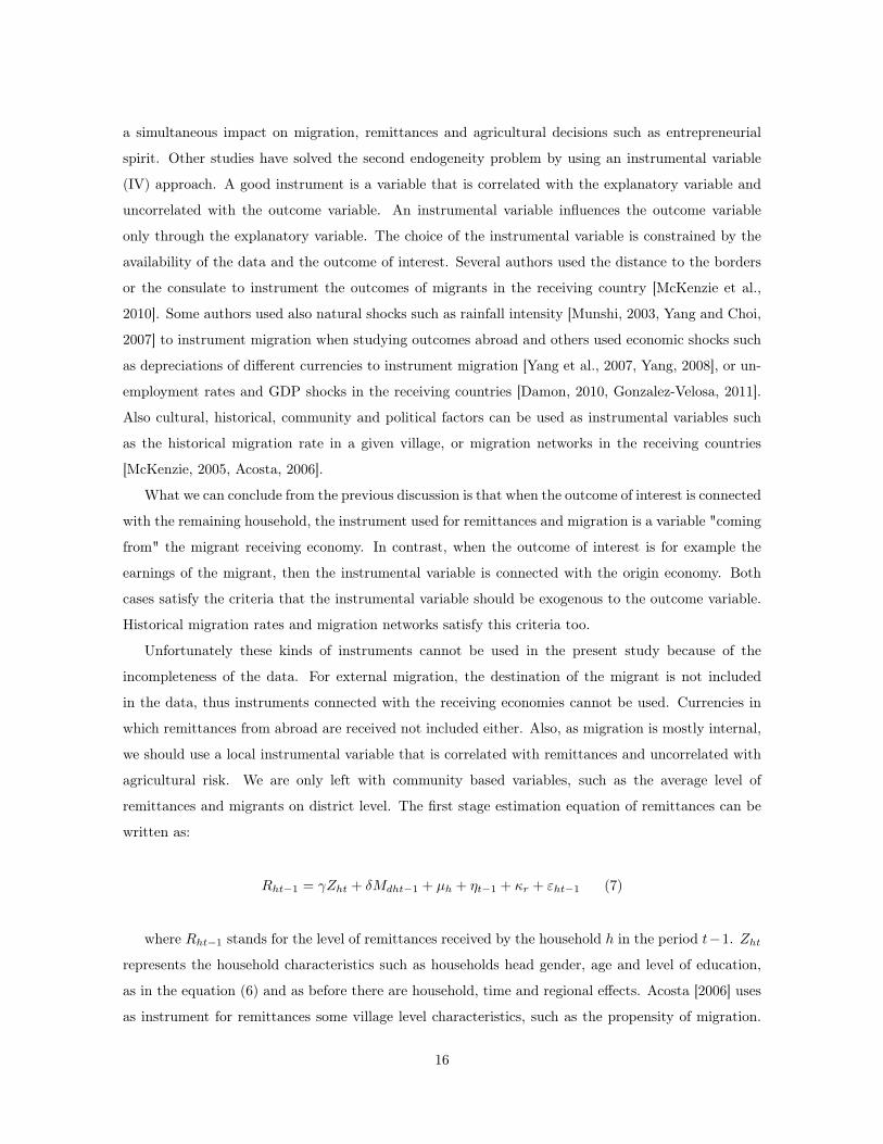
Unfortunately these kinds of instruments cannot be used in the present study because of the

incompleteness of the data. For external migration, the destination of the migrant is not included

in the data, thus instruments connected with the receiving economies cannot be used. Currencies in

which remittances from abroad are received not included either. Also, as migration is mostly internal,

we should use a local instrumental variable that is correlated with remittances and uncorrelated with

agricultural risk. We are only left with community based variables, such as the average level of

remittances and migrants on district level. The first stage estimation equation of remittances can be

written as:

Rht−1 = γZht + δMdht−1 + µh + ηt−1 + κr + εht−1 (7)

where Rht−1 stands for the level of remittances received by the household h in the period t−1. Zht

represents the household characteristics such as households head gender, age and level of education,

as in the equation (6) and as before there are household, time and regional effects. Acosta [2006] uses

as instrument for remittances some village level characteristics, such as the propensity of migration.

16

It is expected that individual remittances increase with district level of migration. As migration is a

prior condition for receving remittances, districts with higher level of remittances are those that have

higher level of migrants. The district level of migrants is represented by the variable Mdht−1 where d

referes to the district where the households h lived in time t− 1. Equation (7) will be estimated using

a Tobit model, as remittances are observed only for a third of the sample. A linear prediction of Rht−1

is introduced in the second stage of the estimation, equation 6.

The third endogeneity problem is reverse causality which may also exist if households that are prone

to risk taking send a migrant once they have made their agricultural decision and expect remittances

in return. The latter case of endogeneity is avoided as the lagged value of remittances is used in the

equation (6).

Another technical problem arises in this case as the diversity indices (Inverse Simpson, Shannon

and Berger-Parker index), and to some extent the portfolio beta, are left-censored. This requires a

Tobit which is a censoring model applied to the linear model with normal residuals. Once again, using

OLS estimation for a censored outcome variable will lead to biased results. Also the count index n

is categorical variable that takes limited number of values. The Poisson estimation model deals with

this kind of dependent variables. The nonlinearity of the different models does not allow the use of

fixed effects. The number of censored observations in the sample is around three percent. Using a

panel model can also be appropriate as it allows to purge the unobservable time invariable household

characteristics.

5 The Results

The First Stage regression (Table 8) confirms that the district average level of migrants has a positive

and significant impact on the level of remittances received by households. The magnitude of the result

is similar for both: the first stage estimation of remittances used as explanatory variable in the risk

portfolio beta estimation and the first stage estimation of remittances used as explanatory variable

in the diversity indices estimation. Table 9 shows the marginal effects for remittances for an average

household. On average, an increase of the district (to which an average household h belongs) mean level

of migrants by one additional migrant of the district mean of migrants increases the level of remittances

by 178 300 Shs. 5 This result is significant at one percent level which gives insights about the validity

of the instrument. A Durbin–Wu–Hausman test is done in order to test endogeneity of remittances,

which verifies whether it is necessay to use an IV strategy or simple Panel estimation is consistent.

The results show that using Panel estimation is not consistent in the case of diversity indices, but5the level of remittances is scaled in order to have a better interpretation of the results; each variable is divided by

10 000 Shs.

17

however we can use the panel estimation results when considering the portfolio beta estimation.

5.1 The impact of remittances on interspecific crop diversification

The regression results for equation (6) are in Table 10. The Tobit-IV and Panel-IV results show

that the level of remittances influences negatively the level of richness and evenness of different crops

cultivated by the farmers, but this result is insignificant. However, we observe for the three categories

od diversity indices that an interaction variable composed of the binary variable credit constraint and

the level of predicted remittances has a negative impact on these diversity indices. Receiving 10000

Shs remittances for households that are credit constraint lowers the level of richness by 0.004 crops at

significant level of 10 percent (Tabel 13), the level of relative abundance by 0.004 points (Table 12,

Inverse Simpson index) and absolute abundance of different crops by 0.003 (Tabel 13, Berger-Parker

index). In other words, remittances push credit-constrained farmers into crop specialisation, thus can

be considered as risk-increasing strategy. This can be interpreted as a wealth effect of remittances that

encourages constrained farmers to engage in crop specialisation.

There are few socio-economic factors that influence the household’s decision in terms of crop di-

versification. First, I observe that an increase of the land size of 1 ha decreases the relative abundance

of crops by 0.01 points at significance level of 1 percent. The interpretation of this result might be

linked to an existence of economies of scale on farm crop cultivation of the sample. This result is

also confirmed by the Berger-Parker index estimation, an increase of land of 1 ha increases the weight

of the most cultivated crop at significance level of 1 percent. As expected, land size as production

factor seems to have an important influence on crop management decisions regardless of the estimation

strategy. Second, if we consider the Panel FE estimation, higher number of plots with different soil

texture, that a farmer owns, reduces the relative and absolute abundance of by 0.18 and 0.09 points,

which is opposite of what was expected initially. If we compare the different indices that include

weights in their computation to the count index, we observe that both categories are influenced by

different factors in the panel/poisson analysis. The number of adults of the household that is a proxy

for labour endowment of the household influences positively the number of crops, but not the diversity

measurements that include weights.

If we consider the tobit estimation on the different indices, we observe that higher labour endowment

and higher dependency ratio are influencing positively the predicted value of richness, evenness and

absolute abundance of crops, which goes in line with the intuition. There is no diversity decision

difference between male and female household’s head. More educated household’s heads engage in

higher crop diversity as they might have more knowledge about the benefits of diversification and

consequences of crop specialisation. Finally, farmers with higher number of plots with different slopes

18

have higher predicted value of relative and absolute abundance. It is important to note that all

these factors are no longer significant in the panel FE analysis, as they might be correlated with the

individual effect.

The cropping season categorical variable(s) indicates that households for which we have observations

only for the 1st or 2nd cropping period have a lower level of crop diversity (from every aspect) than

households for which we have observations for both cropping seasons, although the dependent variable

is based on an average of the two seasons. An intuitive result concerning regions is that, households

coming from the Northern, Eastern and Western regions of Uganda have lower predicted degree of

diversity compared to the Central (Southern) region where the capital city belongs, as the rainfall

and land pattern are such that lower number of crops are cultivated in these regions especially in the

North where pastoral activities are the most common and where the lands are of poor quality; also

the rainfall level is lower and there is a lack of infrastructure compared to the Central region.

5.2 The impact of remittances on the riskiness of the crop portfolio

The results of the model studying the relationship between the riskiness of a crop portfolio and

remittances are less significant than the previous results. Remittances have a positive but statistically

insignificant effect on the level of the portfolio beta (we will focuse on Table 13 as the DWH test states

that there remittances are exogenous enough). According to the panel fixed effect estimation, having a

household’s head that is male inceases the risk index by 0.142 points than having a female household’s

head. Also, a household head that has primary education has a risk portfolio index that is 0.0721 lower

than household with a head that does not have any education. This result seems coherent with the

initial intuition, as we expect that more educated members of the households should be more aware of

the consequences of undertaking more risky activities.

Considering the tobit estimation that allow for regional effects, we observe similar significant re-

gional results as in the case of the diversity indices. In the Northern and Eastern region, households

cultivate less crops and lower-risk drought resistant crops then in the Central region. More precisely,

a household that lives in the Northern region has a predicted value of the portfolio beta that is 0.1

points lower than a household in the Central region. Another intuitive result coming from the tobit

estimation model is that the level of land ownings increases the predicted level of the portfolio beta

which goes in line with the assumption that wealthier households are able to better smooth consump-

tion or income shocks and thus they are better placed when undertaking higher risk/higher income

activities. If we compare the results to the previous section, we observe that increase of land ownings

increase riskiness in terms of crop choice and crop specialisation. Once again, we can more be confident

about the panel estimation as the tobit estimation do not deal with unobserved heterogeneity and the

19

number of censored observations is under three percent. In the Panel estimation, suprisingly we do

not find other significant factors that influence the risk prortfolio. In the next section, we disscuss the

possible explanation of this case.

6 Conclusion

In order to sum up the different results, I relay on the Panel (IV) estimation regarding the

diversity indices as it purges the "unobservable" household characteristic and there very few censored

observations, eventough by definition a Tobit estimation should be used. The main significant findings

in the present study are that remittances alone do no have a significant impact neither on risk choices

nor on crop diversification. This result is probably a matter of the low amount of remittances that

households receive. However, when remittances are interacted with credit status of the household,

crop specialisation is more observed for credit constrained households. This can be interpreted as a

wealth effect for the constrained households, which was not found in the literature. The major question

that arises is to discover whether households engages in low-risk crop specialisation or high-risk crop

specialisation. By running a simple correlation between the riskiness of crop portfolio and the diversity

indices, I find a positive but week correlation (0.05), thus no conclusions can be made and the questions

stays open for further analysis. Also, migration and remittances can be seen as a risky strategy as the

outcomes from these kinds of income diversification are not certain. Including the degree of certainty

of remittances can give some new insights.

An additional result is that different production factors (labour and land) do affect separately the

number and the weight of crops. Labour seems to be significant for the household’s choice if the

number of crops and land size seems to be a key factor for the distribution of weights among different

crops. I find significant difference crop choices in terms of risk between male and female heads of

households. There is also some evidence that head of households that have primary education have

lower-risk decisions compared to non-educated household heads. However this is no longer true for

higher levels of education.

Concerning the insignificance of different factors for the risk crop choices, limited variability of the

portfolio beta variable may be an explanation for two reasons. The first reason is that the individual

crop riskiness is not time varying so if a household that cultivates the same crops in the two periods

and if the weights of these crops do not change significantly, then the portfolio beta will not differ

between the periods. The second reason is that the two waves in this analysis are consecutive, thus we

cannot expect that farmers easily make different decisions on what to crop. Since making different crop

decisions may take time, the invariability of the dependent variable may be due to the consecutiveness

of the waves and the invariability of the crop risk measure. A dataset that includes higher number

20

of periods in the surveys or a longer gap between the periods will be more suitable to analyse the

portfolio beta.

As the results of the impact of remittances on the riskiness of the crop choice are not significant,

we cannot conclude that remittances help farmers to undertake riskier activities that yield higher

incomes and help them to avoid or escape poverty traps. The only result(s) that we can discus is that

remittances lead to crop specialization for credit constrained households. On the one hand, Ugandan

agriculture is mostly rain-fed and relying only on one low-risk crop can lead farmers into a poverty

trap. Instead, higher diversity in crops that have different resistance to weather shocks should be a

better solution when adapting to irregular weather conditions. This strategy seems more appropriate

when dealing with the consequences of climate change. On the other hand, crop specialization can

yield economics of scale. A cost/benefit study on whether crop diversification or crop specialization in

riskier crops is the most beneficial can be done by agro ecological zone in future research in order to

evaluate if remittances contribute to undertake the right strategy. Also the analysis can be extended to

interspecific diversity, by using different crop varieties that can have different impact on risk behaviour.

21

Table 8: Tobit First Stage Estimation

VARIABLES Porfolio Beta Diversity indices

Mean district level of migrants 21.88*** 21.83***(8.049) (8.049)

land 0.00441 -0.00392(0.149) (0.150)

adults 3.517*** 3.466***(0.900) (0.901)

dep ratio 1.181 1.159(1.116) (1.116)

male hh head -55.99*** -56.19***(3.446) (3.451)

age 0.961*** 0.969***(0.104) (0.104)

primary education 18.36*** 18.40***(4.069) (4.069)

secondary education 30.96*** 30.92***(5.741) (5.741)

post secondary training 34.71*** 34.74***(6.061) (6.062)

higher education 110.5*** 110.7***(14.08) (14.09)

1st cropping season -2.962 -2.924(3.769) (3.771)

2nd cropping season 1.926 1.925(4.316) (4.316)

Eastern region -7.471* -7.424*(4.248) (4.248)

Northen region -8.853** -9.077**(4.349) (4.356)

Westren region -32.88*** -33.43***(4.773) (4.799)

non agricultural income 1.23e-07 1.15e-07(2.09e-07) (2.09e-07)

assets 1.83e-07*** 1.83e-07***(2.98e-08) (2.98e-08)

credit constraint -0.132 0.0217(3.019) (3.020)

soil quality index 3.304 3.254(2.634) (2.634)

number of plots with different texture 0.970(4.685)

number of plots with different slope 3.809(3.165)

Constant -74.23*** -79.98***(9.677) (11.09)

Number of hhid 1,849 1,849

22

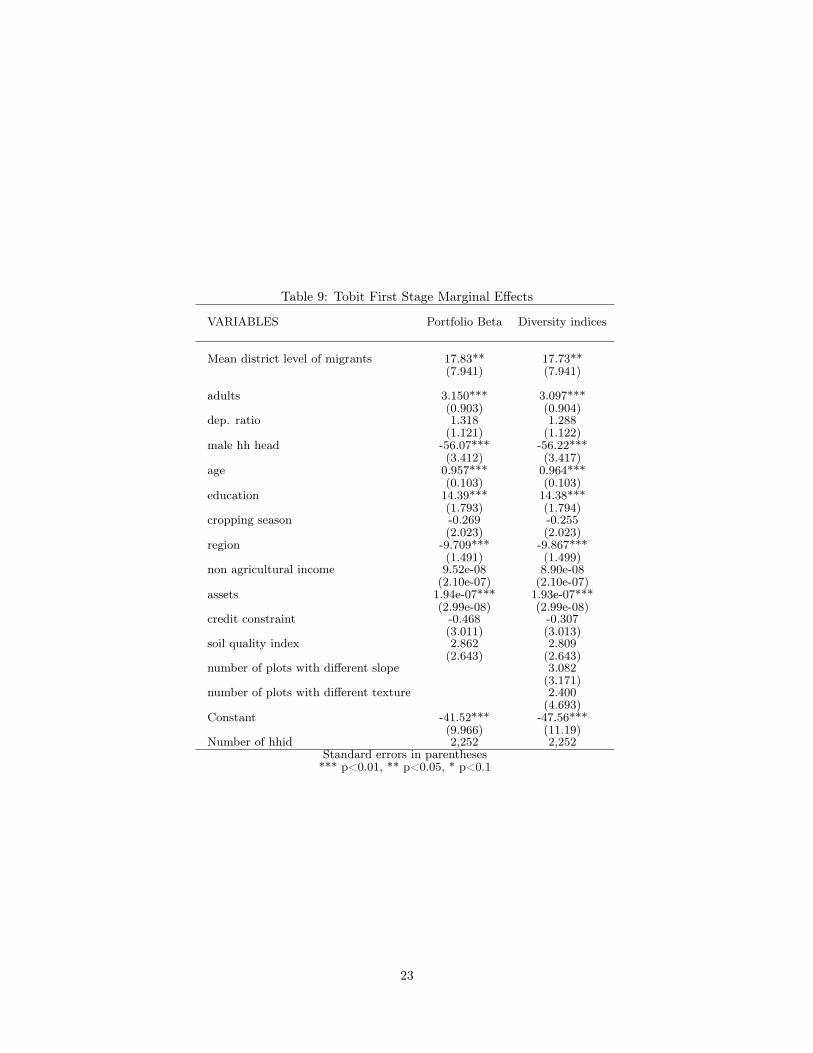
Table 9: Tobit First Stage Marginal Effects

VARIABLES Portfolio Beta Diversity indices

Mean district level of migrants 17.83** 17.73**(7.941) (7.941)

adults 3.150*** 3.097***(0.903) (0.904)

dep. ratio 1.318 1.288(1.121) (1.122)

male hh head -56.07*** -56.22***(3.412) (3.417)

age 0.957*** 0.964***(0.103) (0.103)

education 14.39*** 14.38***(1.793) (1.794)

cropping season -0.269 -0.255(2.023) (2.023)

region -9.709*** -9.867***(1.491) (1.499)

non agricultural income 9.52e-08 8.90e-08(2.10e-07) (2.10e-07)

assets 1.94e-07*** 1.93e-07***(2.99e-08) (2.99e-08)

credit constraint -0.468 -0.307(3.011) (3.013)

soil quality index 2.862 2.809(2.643) (2.643)

number of plots with different slope 3.082(3.171)

number of plots with different texture 2.400(4.693)

Constant -41.52*** -47.56***(9.966) (11.19)

Number of hhid 2,252 2,252Standard errors in parentheses*** p<0.01, ** p<0.05, * p<0.1

23

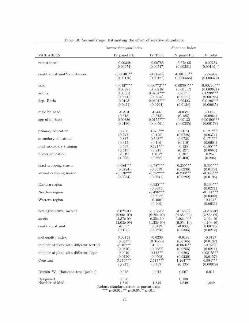
Table 10: Second stage: Estimating the effect of relative abundance

Inverse Simpson Index Shannon Index

VARIABLES IV panel FE IV Tobit IV panel FE IV Tobit

remittances -0.00348 -0.00785 -5.57e-05 -0.00234(0.00974) (0.00547) (0.00281) (0.00169) )

credit constraint*remittances -0.00401** -3.11e-05 -0.00113** 5.27e-05(0.00176) (0.00121) (0.000565) (0.000372)

land -0.0127*** -0.00772*** -0.00394*** -0.00226***(0.00381) (0.00218) (0.00117) (0.000671)

adults 0.00653 0.0754*** 0.0171 0.0298***(0.0560) (0.0255) (0.0171) (0.00788)

dep. Ratio 0.0193 0.0591*** 0.00423 0.0196***(0.0421) (0.0204) (0.0124) (0.00635)

male hh head -0.310 -0.447 -0.0383 -0.132(0.615) (0.313) (0.185) (0.0964)

age of hh head 0.00336 0.0155*** 0.00132 0.00490***(0.0130) (0.00561) (0.00335) (0.00173)

primary education 0.288 0.373*** 0.0673 0.121***(0.247) (0.120) (0.0728) (0.0371)

secondary education 0.337 0.503** 0.0738 0.171***(0.375) (0.196) (0.110) (0.0604)

post secondary training 0.597 0.621*** 0.125 0.185***(0.417) (0.215) (0.127) (0.0663)

higher education 2.019 1.107* 0.387 0.257(1.328) (0.668) (0.400) (0.206)

fisrst cropping season -0.684*** -0.787*** -0.255*** -0.305***(0.0724) (0.0579) (0.0236) (0.0178)

second cropping season -0.530*** -0.752*** -0.238*** -0.305***(0.0954) (0.0641) (0.0292) (0.0196)

Eastern region -0.325*** -0.109***(0.0871) (0.0271)

Northen region -0.496*** -0.141***(0.0972) (0.0302)

Western region -0.400* -0.124*(0.206) (0.0636)

non agricultural income 8.62e-09 -1.13e-08 3.76e-09 -4.31e-09(9.96e-09) (9.28e-09) (4.65e-09) (2.85e-09)

assets 3.37e-09 6.35e-10 1.02e-09* 2.92e-10(2.03e-09) (1.33e-09) (6.05e-10) (4.10e-10)

credit constraint -0.117 0.0139 -0.0383 0.00776(0.105) (0.0690) (0.0335) (0.0212)

soil quality index 0.00755 -0.0238 -0.0188 -0.0127(0.0577) (0.0429)) (0.0165) (0.0132)

number of plots with different texture -0.187** -0.111 -0.0604** -0.0263(0.0870) (0.0687) (0.0255) (0.0211)

number of plots with different slope 0.0949 0.113** 0.0203 0.0515***(0.0750) (0.0508) (0.0220) (0.0157)

Constant 3.174*** 2.517*** 1.264*** 0.994***(0.943) (0.439) (0.135) (0.00929)

Durbin–Wu–Hausman test (pvalue) 0.045 0.012 0.067 0.011

R-squared 0.096 0.138Number of hhid 1,849 1,849 1,849 1,849

Robust standard errors in parentheses*** p<0.01, ** p<0.05, * p<0.1

24

Table 11: Second stage: Estimating the effect of richness and absolute abundance

Count Index Berger Parker Index

VARIABLES IV Panel FE IV Poisson FE IV panel FE IV Tobit

remittances -0.00357 -0.000232 -0.00285 -0.00593(0.00998) (0.00327) (0.00538) (0.00363)

credit constraint*remittances -0.00399* -0.000820 -0.00332*** -0.000204(0.00207) (0.000669) (0.00111) (0.000807)

land -0.00349 -0.000497 -0.00862*** -0.00582***(0.00406) (0.00123) (0.00219) (0.00146)

adults 0.258*** 0.0474* -0.0287 0.0374**(0.0810) (0.0260) (0.0437) (0.0167)

dep. ratio 0.0644 0.00975 -0.00222 0.0299**(0.0570) (0.0186) (0.0308) (0.0133)

male hh head -0.414 -0.0657 -0.228 -0.359*(0.616) (0.203) (0.333) (0.207)

age hh head 0.0196 0.00347 0.00153 0.00951**(0.0140) (0.00456) (0.00757) (0.00371)

primary education 0.450* 0.0783 0.202 0.225***(0.258) (0.0845) (0.139) (0.0793)

secondary education 0.541 0.0991 0.205 0.303**(0.432) (0.142) (0.233) (0.129)

post secondary training 0.526 0.0857 0.359 0.378***(0.467) (0.155) (0.252) (0.142)

higher education 0.845 0.128 1.569** 0.856*(1.410) (0.490) (0.761) (0.441) )

first cropping season -1.067*** -0.225*** -0.382*** -0.404***(0.0990) (0.0333) (0.0534) (0.0386)

second cropping season -1.141*** -0.239*** -0.256*** -0.390***(0.103) (0.0343) (0.0554) (0.0430)

Eastern Region -0.168***(0.0562) )

Northen region -0.325***(0.0631)

Western region -0.277**(0.136)

non agricultural income 3.39e-08** 7.81e-09 1.21e-10 -6.28e-09(1.67e-08) (5.67e-09) (8.99e-09) (6.16e-09)

assets 4.61e-09* 8.38e-10 2.75e-09* 8.04e-10(2.68e-09) (8.69e-10) (1.45e-09) (8.76e-10)

credit constraint -0.0971 -0.0182 -0.116* 0.00811(0.117) (0.0375) (0.0633) (0.0461)

soil quality index -0.0671 -0.0166 0.0159 -0.0143(0.0733) (0.0236) (0.0396) (0.0287)

number of plots with different texture -0.0969 -0.0211 -0.120** -0.0896*(0.109) (0.0341) (0.0588) (0.0462)

number of plots with different slope 0.0782 0.0119 0.0759 0.0600*(0.0909) (0.0292) (0.0490) (0.0338)

Constant 3.438*** 2.367*** 1.952***(1.081) (0.584) (0.290)

Durbin–Wu–Hausman test (pvalue) 0.121 0.111 0.051 0.008

R-squared 0.135 0.070Number of hhid 1,849 1,688 1,849 1,849

Standard errors in parentheses*** p<0.01, ** p<0.05, * p<0.1

25

Table 12: Second stage: Portfolio Beta

VARIABLES IV Panel FE IV Tobit

remittances -0.000560 -0.000801(0.00243) (0.00179)

credit constraint*remittances -1.25e-06 -2.63e-05(0.000319) (0.000386)

land 0.000824 0.00133*(0.00160) (0.000707)

adults 0.0189 0.00389(0.0185) (0.00906)

dep. ratio 0.00648 -0.000389(0.0110) (0.00743)

male hh head 0.111 0.0236(0.172) (0.103)

age 0.00185 -0.000253(0.00283) (0.00187)

primary education -0.0634 -0.0554(0.0818) (0.0407)

secondary education 0.0184 -0.0211(0.110) (0.0663)

post secondary training 0.00412 0.0226(0.136) (0.0724)

higher education 0.0862 -0.0195(0.319) (0.224)

1st cropping season -0.0302 -0.0152(0.0243) (0.0185)

second cropping season -0.0322 -0.0431**(0.0259) (0.0200)

Eastern region -0.131***(0.0339)

Northen region -0.100***(0.0363)

Wester region 0.0477(0.0691)

non agricultural income -4.33e-10 -2.05e-09(1.71e-09) (3.01e-09)

assets 5.04e-10 4.33e-10(6.04e-10) (4.48e-10)

credit constraint 0.000377 0.00611(0.0125) (0.0220)

quality index 0.00478 0.0118Constant 0.0705 0.311**

(0.240) (0.135) )

Durbin–Wu–Hausman test (pvalue) 0.900 0.121

R-squared 0.013Number of hhid 1,849 1,849

Standard errors in parentheses*** p<0.01, ** p<0.05, * p<0.1

26

Table 13: Estimation Portfolio Beta

VARIABLES Panel FE Tobit

Remittances 0.000106 1.29e-05(0.000306) (0.000238)

credit constraint*remittances -0.000358 -0.000138(0.000407) (0.000323)

land 0.000820 0.00120*(0.000883) (0.000695)

adults 0.0182 0.00706(0.0156) (0.00581)

dep. ratio 0.00615 0.000368(0.0120) (0.00661)

male hh head 0.142*** 0.0594***(0.0549) (0.0217)

age 0.00127 -0.000932(0.00216) (0.000655)

primary education -0.0721* -0.0690***(0.0399) (0.0231)

secondary education 0.00367 -0.0372(0.0643) (0.0331)

post secondary training education -0.0134 -0.0209(0.0678) (0.0347)

higher education 0.0273 -0.118(0.182) (0.0932)

1st cropping season -0.0289 -0.0201(0.0209) (0.0173)

2nd cropping subwave -0.0328 -0.0553***(0.0220) (0.0192)

Eastern region 0 -0.103***(0) (0.0282)

Northen region 0 -0.0805***(0) (0.0293)

Western region 0 0.0875***(0) (0.0293)

nonagricultural income -6.11e-10 -1.38e-09(3.61e-09) (1.32e-09)

assets 4.06e-10 1.66e-10(4.13e-10) (1.98e-10)

credit constraint 0.00409 0.0142(0.0168) (0.0142)

Constant 0.112 0.346***(0.129) (0.0515)

R-squared 0.013Number of hhid 1,849 1,849

Standard errors in parentheses*** p<0.01, ** p<0.05, * p<0.1

27

References

Pablo Acosta. Labor supply, school attendance, and remittances from international migration: the

case of el salvador. World Bank Policy Research Working Paper, (3903), 2006.

Stefan Baumgärtner. Measuring the diversity of what? and for what purpose? a conceptual comparison

of ecological and economic measures of biodiversity. Interdisciplinary Institute for Environmental

Economics, Heidelberg, 2004.

Mintewab Bezabih and Salvatore Di Falco. Rainfall variability and food crop portfolio choice: evidence

from ethiopia. Food Security, 4(4):557–567, 2012.

Romina Cavatassi, Leslie Lipper, and Paul Winters. Sowing the seeds of social relations: social capital

and agricultural diversity in hararghe ethiopia. Environment and Development Economics, 17(05):

547–578, 2012.

Amy Lynne Damon. Agricultural land use and asset accumulation in migrant households: the case of

el salvador. The Journal of Development Studies, 46(1):162–189, 2010.

FAOSTAT. Food and agriculture organization of the united nations, faostat database, 2011.

Carolina Gonzalez-Velosa. The effects of emigration and remittances on agriculture: evidence

from the philippines. Job market paper (available at http://econweb. umd. edu/˜ gonzalez-

velosa/JMP_Gonzalezvelosa_JAN. pdf), 2011.

Flore Gubert. Do migrants insure those who stay behind? evidence from the kayes area (western mali).

Oxford Development Studies, 30(3):267–287, 2002.

David McKenzie. Beyond remittances: the effects of migration on mexican households. International

migration, remittances and the brain drain, McMillan and Palgrave, pages 123–47, 2005.

David McKenzie, Steven Stillman, and John Gibson. How important is selection? experimental vs.

non-experimental measures of the income gains from migration. Journal of the European Economic

Association, 8(4):913–945, 2010.

Mariapia Mendola. Migration and technological change in rural households: Complements or substi-

tutes? Journal of Development Economics, 85(1):150–175, 2008.

Kaivan Munshi. Networks in the modern economy: Mexican migrants in the us labor market. The

Quarterly Journal of Economics, 118(2):549–599, 2003.

Susan M Richter. The insurance role of remittances on household credit demand. In American

Agricultural Economics Association Annual Meeting, July, pages 27–29, 2008.

28

Oded Stark. The migration of labor. Blackwell Oxford, 1991.

Oded Stark and David Levhari. On migration and risk in ldcs. Economic Development and Cultural

Change, 31(1):191–196, 1982.

Calum G Turvey. Regional and farm-level risk analyses with the single-index model. Northeastern

Journal of Agricultural and Resource Economics, 20(2), 1991.

World Bank. Migration and remittances factbook 2011. Development Prospects Group, 2010.

World Bank. Development indicators, agricultureagriculture : avaliable at

http://data.worldbank.org/indicator/nv.agr.totl.zs/countries, 2011.

World Bank. Migration and development brief 20. Development Prospects Group, 2013.

Dean Yang. International migration, remittances and household investment: Evidence from philippine

migrants’ exchange rate shocks. The Economic Journal, 118(528):591–630, 2008.

Dean Yang and HwaJung Choi. Are remittances insurance? evidence from rainfall shocks in the

philippines. The World Bank Economic Review, 21(2):219–248, 2007.

Dean Yang, A Martínez, et al. Remittances and poverty in migrants’ home areas: Evidence from the

philippines. Working Paper, University of Chile, 2007.

29