agricultural technology adoption and rural poverty
TRANSCRIPT

1
Agricultural Technology Adoption and Rural Poverty: Application of an
Endogenous Switching Regression for Selected East African Countries
Solomon Asfaw1* and Bekele Shiferaw2
1* Corresponding author, International Crops Research Institute for the Semi-Arid Tropics (ICRISAT), UN
Avenue, Gigiri, PO Box 39063-00623, Nairobi, Kenya. Tel: +254207224551; Fax: +254207224001; E-mail:
[email protected] 2 International Maize and Wheat Improvement Centre (CIMMYT), UN Avenue, Gigiri PO. Box, 30677-00100
Nairobi, Kenya.
May 27, 2010 (First Version)
Abstract
Achieving agricultural growth and development and thereby improving rural household welfare will require increased efforts to provide yield enhancing and natural resources conserving technologies. Agricultural research and technological improvements are therefore crucial to increase agricultural productivity and thereby reduce poverty. However evaluation of the impact of these technologies on rural household welfare have been very limited by lack of appropriate methods and most of previous research has therefore failed to move beyond estimating economic surplus and return to research investment. This paper evaluates the potential impact of adoption of modern agricultural technologies on rural household welfare measured by crop income and consumption expenditure in rural Ethiopia and Tanzania. The study utilizes cross-sectional farm household level data collected in 2007 from a randomly selected sample of 1313 households (700 in Ethiopia and 613 in Tanzania). We estimate the casual impact of technology adoption by utilizing endogenous switching regression and propensity score matching methods to assess results robustness. This helps us estimate the true welfare effect of technology adoption by controlling for the role of selection problem on production and adoption decisions. Our analysis reveals that adoption of improved agricultural technologies has a significant positive impact on crop income although the impact on consumption expenditure is mixed. This confirms the potential direct role of technology adoption on improving rural household welfare, as higher incomes from improved technology translate into lower income poverty. JEL classification: C13, C15, O32, O38 Key words: rural household welfare, technology adoption, propensity score matching, endogenous switching, Ethiopia, Tanzania

2
1. Introduction
In much of Sub-Saharan Africa, agriculture is a strong option for spurring growth, overcoming
poverty, and enhancing food security. Of the total population of Sub-Saharan Africa in 2003,
66% lived in rural areas and more than 90% of rural people in these regions depend on
agriculture for their livelihoods. Improving the productivity, profitability, and sustainability of
smallholder farming is therefore the main pathway out of poverty in using agriculture for
development (WDR, 2008). Achieving agricultural productivity growth will not be possible
without developing and disseminating yield-increasing technologies because it is no longer
possible to meet the needs of increasing numbers of people by expanding areas under
cultivation. Agricultural research and technological improvements are therefore crucial to
increase agricultural productivity and thereby reduce poverty and meet demands for food
without irreversible degradation of the natural resource base.
Agricultural research can contribute to poverty reduction in three major ways. First,
agricultural research helps in developing yield-increasing technologies contributing to an
increase in the supply of food on which the poor spend a considerable share of their income.
The development of high-yielding varieties, which boost food production both by increasing
yields per unit of land per cropping season and by facilitating multiple cropping, must remain a
critical component of the research strategy to achieve first Millennium Development Goal
(MDG 1) of halving poverty by 2015. Second, agricultural research help to conserve natural
resources since the poor lack alternative means to intensify agriculture except forced to overuse
or misuse the natural resource bases to meet basic needs. Third, because the poor tend to reside
in unfavoured or marginal agricultural areas, research should aim at developing technologies
suitable for these. However, it is widely argued that research often neglected the unfavoured
areas, thereby worsening poverty in them by reducing market prices of grains without
improving technology (Lipton and Longhurst, 1989). The question remains, however, as to
what types of technology are suitable for marginal areas. What kinds of research have high
expected payoffs in terms of income generation and, hence, poverty reduction in such areas?
In the face of increasing variability of economic and agro-climatic conditions in the
semi-arid tropical countries in Africa, dryland legumes like chickpea, pigeonpea and peanuts
presents an opportunity in reversing the trends in productivity, poverty and food insecurity. In
part, this is because legumes have the capacity to fix atmospheric nitrogen in soils and thus

3
improves soil fertility and save fertilizer costs in subsequent crops. Second, it improves more
intensive and productive use of land, particularly in areas where land is scarce and the crop can
be grown as a second crop using residual moisture. Third, it reduces malnutrition and improves
human health especially for the poor who cannot afford livestock products. Fourth, the growing
demand in both the domestic and export markets provides a source of cash for smallholder
producers.
Despite the crucial role of dryland legumes for poverty reduction and food security in
semi-arid tropics, lack of technological change and market imperfections have often locked
small producers into subsistence production and contributed to stagnation of the sector
(Shiferaw and Teklewold, 2007). Often the traditional variety dominates the local and export
markets, however; low productivity of the variety limits the farmers’ competitiveness in these
markets. To harness the untapped potential of legumes for the poor, the national agricultural
research organization of Ethiopia in collaboration with International Crops Research Institute
for the Semi-Arid Tropics (ICRISAT) have developed and released several high-yielding and
stress tolerant varieties of chickpea with desirable agronomic and market traits. A total of 11
improved chickpea varieties had been released as a result of this research program. In
Tanzania, a screening program for fusarium resistance was initiated as a concerted effort
between ICRISAT and Tanzania researchers in the early 1990s. The main trust was to identify
disease resistant types that combine market and farmer-preferred traits. This effort resulted in
development of two fusarium-resistant improved pigeonpea among 21 varieties that were
successfully tested on station, which are becoming popular in Tanzania (Shiferaw et al., 2008).
The underlying objectives of such undertakings are to reduce hunger, malnutrition,
poverty and increase the incomes of poor people living in drought-prone areas of Sub-Saharan
Africa. However, evaluating of the impact of these improved technologies on household
welfare outcomes have been very limited by lack of appropriate methods and most of previous
research has therefore failed to move beyond estimating economic surplus and return to
research investment. Thus using farm-level data collected from a random cross-section sample
of 1313 small-scale producers (700 in Ethiopia and 613 in Tanzania), the objective of this
paper is to provide rigorous empirical evidence on the role of improved chickpea and
pigeonpea technology adoption on household welfare outcomes measured by crop income and
consumption expenditure in rural Ethiopia and Tanzania.

4
From an econometric standpoint analyzing the welfare implications of agricultural
technology poses at least two challenges: unobserved heterogeneity and possible endogeneity.
There seems to be a two-way link between technology adoption and household well-being.
Technology adoption may result in productivity enhancement for small producers and greater
income, but it may also be that greater income leads to more technology adoption. In this
paper, we take into account that the differences in welfare outcome variables between those
farm households that did and those that did not adopt improved technology could be due to
unobserved heterogeneity. Not distinguishing between the casual effect of technology adoption
and the effect of unobserved heterogeneity could, indeed, lead to misleading policy
implications. We account for the endogeneity of the adoption decision (that is, for the
heterogeneity in the decision to adopt or not to adopt new technology and for unobservable
characteristics of farmers and their farm) by estimating a simultaneous equations model with
endogenous switching by full information maximum likelihood estimation. We also employed
non-parametric regression method (propensity score matching) to assess the robustness of the
results.
This paper aims to contribute to the literature by providing a micro perspective on the
impact of agricultural technology. Assessing the impact of farm technology adoption can assist
with setting priorities, providing feedback to the research programs, guide policy makers and
those involved in technology transfer to have a better understanding of the way new
technologies are assimilated and diffused into farming communities, and show evidence that
clients benefit from the research products (Manyong et al., 2001). Now days there is clear
demand for greater institutionalization of impact assessment and impact culture with a better
understanding of the complexities of the links between agricultural technology and poverty.
The remainder of the paper is organized as follows. Section two provides overview
about chickpea and pigeonpea production system in Ethiopia and Tanzania. Section three
present the survey design and data. Section four shows the econometric model used for
estimation. Section five presents the estimation results and in section six conclusions are drawn
and some further implications are noted.

5
2. Overview of chickpea and pigeonpea production system in East Africa
Ethiopia is the largest producer of chickpea in Africa accounting for about 46% of the
continent’s production during 1994-2006 (FAOSTAT). It is also the seventh largest producer
worldwide and contributes about 2% to the total world chickpea production. Chickpea, locally
known as shimbra, is one of the major pulse crops (including faba bean, field pea, haricot bean,
lentil and grass pea) in Ethiopia and in terms of production it is the second most important
legume crop after faba beans. It contributed about 16% of the total pulse production during
1999-2008 (CSA). The total annual average (1999-2008) chickpea production is estimated at
about 173 thousand tonnes. During the same period, chickpea was third after faba beans and
field peas in terms of area coverage.
At present the use of improved chickpea production technology packages is negligible.
Over the last three decades (1974-2005), 11 improved chickpea varieties (six kabuli and five
desi) were released in Ethiopia. However, the adoption rate of these varieties is very low.
Official estimates from the Central Statistics Authority (CSA) show that, of the total chickpeas
cultivated area (194,981 ha) only 0.69% was covered by improved chickpea seeds in 2001/02.
The main reasons indicated for low adoption rates are insufficient seed production and
marketing systems that limit the availability of quality improved seeds, lack of credit, late
delivery, and theft during the green stage (Byerlee et al., 2000; Shiferaw et al., 2008).
Although chickpea is widely grown in Ethiopia, the major producing areas are concentrated in
the two regional states - Amhara and Oromia. These two regions cover more than 90% of the
entire chickpea area and constitute about 92% of the total chickpea production (CSA). The top
9 chickpea producing zones (North Gonder, South Gonder, North Shewa, East Gojam, South
Wello, North Wello, West Gojam, Gonder Zuria) belong to the Amhara region and account for
about 80% of the country’s chickpea production. In the Oromia region, the major producing
zones are in West Shewa, East Shewa and North Shewa, which account for about 85% of the
total area and production in this regional state.
Pigeonpea (Cajanus cajan) is another important grain legume widely grown and
adapted to the semi-arid regions of South Asia and Eastern and Southern Africa. The largely
drought tolerant crop allows poor families protect their livelihoods and meet their food and
cash income when most other crops fail in areas with erratic rainfall. Farmers in land-scarce
areas can intensify land use and harvest two crops through inter-cropping with cereals (like

6
maize and sorghum) allowing farmers to diversify risks and maximize their incomes.
Pigeonpea is a tradable crop both in local and international markets, and export demand
(mainly to south Asia) often outstrips supply (Joshi et al., 2001; Lo Monaco, 2003).
Smallholder farmers market a substantial portion of the annual produce to meet their cash
requirements. Tanzania is one of the major growers and exporters of the crop in the region.
Tanzania exports significant amounts (30–40 thousand tons/year) to India, and there is a
growing processing and value-adding industry that would allow the country to export de-hulled
split pea (dhal) to the Far East, Europe, and America. However, the pigeonpea industry in
Tanzania has been affected by poor productivity and limited marketed surplus produce of
smallholder farmers. The poor yields are mainly due to low yielding and disease susceptible
local varieties. Farmers even abandoned production of this important crop mainly due to
fusarium wilt, a fungal soil-borne disease that devastates the crop. Once the field is infested
with the disease, the fungus can stay in the soil for a long period of time, making it very
difficult for poor farmers to control it without the use of extended rotations or expensive
chemicals. The disease is pervasive in all pigeonpea growing areas in east and southern Africa
and spreads among fields through agricultural equipment and field operations (Gwata et al.,
2006).
A screening program for fusarium resistance was initiated as a concerted effort between
ICRISAT and Tanzanian researchers in the early 1990s. The main thrust was to identify
disease resistant types that combine market and farmer-preferred traits. By 1997, this effort
resulted in the development of 21 varieties that were successfully tested on-station, which was
followed by participatory on-farm testing and evaluation of a few promising lines. Two of
these fusarium-resistant improved pigeonpea (FRIP) varieties (ICEAP 00040 and 00053),
which embody farmer and market-preferred traits are becoming popular in northern Tanzania.
3. Survey Design and Data
The data used for this paper originates from a survey conducted by the International Crop
Research Institute for Semi-Arid Tropics (ICRISAT), Ethiopian Institute of Agricultural
Research (EIAR) and Selian Agricultural Research Institute (SARI). The primary survey was
done in two stages. First, a reconnaissance survey was conducted by a team of scientists to
have a broader understanding of the production and marketing conditions in the survey areas.
During this exploratory survey, discussions were held with different stakeholders including

7
farmers, traders and extension staff working directly with farmers. The findings from this stage
were used to refine the study objectives, sampling methods and the survey instrument. The
household survey was then carried out in March 2008 in Ethiopia and from October to
December 2008 in Tanzania. A formal survey instrument was prepared and trained
enumerators collected the information from the households via personal interviews.
A multi-stage sampling procedure was used to select districts, kebeles1 and farm
households. In the first stage, three districts namely Minjar-Shenkora, Gimbichu and Lume-
Ejere were purposively selected from the major legume producing area based on the intensity
of chickpea production, agro-ecology and accessibility. These districts represent one of the
major chickpea growing areas in the country where improved varieties are beginning to be
adopted by farmers. The districts are in the Shewa region in the central highlands of the
country and are located north east of Debre Zeit which is 50 kms south east of the capital,
Addis Ababa. Debre Zeit Agricultural Research Centre (DZARC) is also located in the area
and is a big asset to the districts in terms of information on quality seed, agronomic practices,
marketing, storage, introducing new crop varieties and other relevant information. Chickpea
production in Gimbichu and Lume-Ejere districts ranges from 12,500 to 15,000 ha whereas
chickpea production in Minjar-Shenkora ranges from 15,000 to 17,500 ha per year. The crop is
grown during the post-rainy season on black soils using residual moisture.
A random sample of 8-10 kebeles growing chickpea were selected from each district for
the survey. This was followed by random sampling of 150-300 farm households from each
district. A slightly higher sample was taken from Lume-Ejere district mainly because of large
number of households growing chickpea in this district.
In Tanzania, the sampling framework is based on a multi-stage random sample of
villages in four districts in the Northern zone of Tanzania. In the first stage, four districts
namely Babati, Kondoa, Arumeru and Karatu were selected from the major legumes producing
area based on the intensity of pigeonpea production, agro-ecology and accessibility. These
districts represent one of the major pigeonpea growing areas in the country where improved
varieties are beginning to be adopted by farmers. In each of the four districts three major
divisions were selected giving rise to a total of 12 divisions. Subsequently, two wards were
sampled in each of the selected divisions resulting into a total of 24 wards. Twenty five farmers
1 This refers to peasant associations (rural communities) which represent the lowest administrative unit in the country.

8
were then randomly sampled from a list of farm families in each village and ward. A total of
613 farm households in four districts were surveyed using the standardized survey instrument.
The survey collected valuable information on several factors including household
composition and characteristics, land and non-land farm assets, livestock ownership, household
membership in different rural institutions, varieties and area planted, costs of production, yield
data for different crop types, indicators of access to infrastructure, household market
participation, household income sources and major consumption expenses.
4. Empirical impact evaluation challenges and estimation strategies
4.1 Impact evaluation problem
Estimation of the welfare gain of adoption of agricultural technologies based on non-
experimental observations is not trivial because of the need of finding on counterfactual of
intervention. What we cannot observe is the welfare outcome for those farmers who adopted
improved technology had they not had adopted it (or the converse). In experimental studies,
this problem is addressed by randomly assigning improved seeds to treatment and control
status, which assures that the welfare outcome observed on the control households that adopt
improved technology are statistically representative of what would have occurred without
adoption. However, improved technology is not randomly distributed to the two groups of the
households (adopters and non-adopters), but rather the households themselves deciding to
adopt or not to adopt based on the information they have. Therefore, adopters and non-adopters
may be systematically different.
The simplest approach to examine the impact of adoption of improved technologies on
welfare outcomes would be to include on welfare equation a dummy variable equal to one if
the farm-household adopted new technology, and then, to apply ordinary least squares. This
approach, however, might yield to biased estimates because it assumes that adoption of
improved technology is exogenously determined while it is potentially endogenous. The
decision to adopt or not is voluntary and may be based on individual self-selection. Farmers
that adopted may have systematically different characteristics from the farmers that did not
adopt, and they may have decided to adopt based on expected benefits. Unobservable
characteristics of farmer and their farm may affect both the adoption decision and the welfare
outcome, resulting in inconsistent estimates of the effect of adoption of agricultural technology
on household welfare. For instance, if only the most skilled or motivated farmers choose to

9
adopt and we fail to control for skills, then we will incur in an upward bias. The solution is to
explicitly account for such endogeneity using simultaneous equation models (Hausman, 1978).
The other econometric issue is that even if we account for the endogeneity, it may be
inappropriate to use a pooled sample of adopters and non-adopters (i.e. a dummy regression
model wherein a binary indicator is used to assess the effect of chickpea/pigeonpea technology
adoption on some welfare outcome variables). The question is whether technology adoption
should be assumed to have an average impact over the entire sample of farmers, by way of an
intercept shift, or it should be assumed to raise the productivity of factors of production, by
way of slope shifts in the income function (Alene and Manyong, 2007). Pooled model
estimation assumes that the set of covariates has the same impact on adopters and non-adopters
(i.e. common slope coefficients for both regimes). This implies that technology adoption has
only an intercept shift effect, which is always the same irrespective of the values taken by other
covariates that determine welfare outcome. If it is assumed that factors of production have
differential effects on household welfare outcome, separate welfare outcome functions for
adopters and non-adopters have to be specified, while at the same time accounting for
endogeneity. The econometric problem will thus involve both endogeneity (Hausman 1978)
and sample selection (Heckman 1979). This motivates an endogenous switching regression
model that accounts for both endogeneity and sample selection and allows interactions between
adoption and other covariates in the welfare outcome function (Freeman et al., 2001 and Alene
and Manyong, 2007). Two proxies are used to measure household welfare outcome in this
paper, namely crop income and household consumption expenditure per adult equivalent2.
Thus we estimate two welfare outcome functions for adopters and another for non-adopters. In
addition to switching regression, we also employed non-parametric techniques, namely
propensity score matching (PSM), to overcome the econometric problems and assess the
robustness of our results.
2 Income from crop production is calculated as annual production value of farm products minus paid-out costs, which include costs on seeds, fertilizer, chemicals, hired labor and oxen rental including own oxen. Consumption expenditures captures six major categories including food grains, livestock product (such as meat), vegetables and other food items (such as sugar, salt), beverages (such as coffee, tea leaves), clothing and energy (such as shoes, kerosene) and social activities (contribution to churches or local organization, education and medical expenditure) over the twelve months (2006/07).

10
4.2 Propensity score matching (PSM) methods
The propensity score matching method is one of the non-parametric estimation techniques that
do not depend on functional form and distributional assumptions. The method is intuitively
attractive as it helps in comparing the observed outcomes of technology adopters with the
outcomes of counterfactual non-adopters (Heckman et al., 1998). Despite its heavy data
requirements, the matching method can produce experimental treatment effect results when
such data are not feasible and/or available. It also helps to evaluate programs that require
longitudinal datasets using single cross-sectional dataset where the former does not exist. The
basic idea of the PSM method is to match observations of adopters and non-adopters according
to the predicted propensity of adopting a superior technology (Rosebaum and Rubin 1983:
Heckman et al., 1998; Smith and Todd, 2005; Wooldridge, 2005). The main feature of the
matching procedure is the creation of the conditions of randomized experiment in order to
evaluate a causal effect as in a controlled experiment.
Let iG denotes a dummy variable such that 1iG if the ith individual adopt improved
technology and 0iG otherwise. Similarly let ii YandY 21 denote potential observed welfare
outcomes for adopter and non-adopter units respectively. Then ii YY 21 is the impact of
the technology on the ith individual, usually called treatment effect. As we observe
iiiii YGYGY 21 )1( rather than ii YandY 21 for the same individual, we are unable to
compute the treatment effect for every unit. The primary treatment effect of interest that can be
estimated is therefore the Average impact of Treatment on the Treated (ATT) given by
)1/( 21 iii GYYE (1)
Following Rosenbaum & Rubin (1983), the propensity score can be estimated as
)/1()( XGPXP i (2)
Given the assumptions that (a) XGYY ii /, 21 i.e., the potential outcomes are independent
of technology adoption given X , this imply
))(,0/())(,1/( 22 XPGYEXPGYE ii and (b) 1)(0 XP ,i.e., for all X there
is a positive probability of either adopting )1( G or not adopting )0( G , this guarantees
every adopter a counterpart in the non-adopter population,

11
The ATT can then be estimated as
))(,0/())(,1/(
))(,1/(
)1/(
21
21
21
XPGYEXPGYEE
XPGYYEE
GYYE
iiii
iii
iii
(3)
The propensity score is a continuous variable and there is no way to get adopter with
the same score as its counterfactual(s). Thus, estimation of the propensity score is not sufficient
to compute the average treatment effect given by equation (3). We need to search for
counterfactual(s) that matches with each adopter depending on its propensity score. Different
matching methods are used in the literature (for detail explanations refer Smith and Todd,
2005). We use the nearest-neighbor matching method to pick comparison groups. This method
could use a single nearest-neighbor or multiple nearest-neighbors with the closest propensity
score to the corresponding adopter unit. The method could also be applied with or without
replacement where the former allows a given non-adopter to match with more than one adopter
(Becker and Ichino, 2002; Dehejia and Wahba, 2002). To check the robustness of our result,
the impact estimate calculated using the nearest neighbor matching method is compared to the
estimates of Kernel matching method. As discussed earlier, the observed outcome variable
used as a proxy for the welfare of smallholder farmers, in this paper, are crop income and
household consumption expenditure per adult equivalent.
4.3 Endogenous switching regression models
To complement the PSM techniques and to assess consistency of the results to different
assumptions, endogenous switching regression techniques were applied3. We specify the
selection equation for technology adoption as
iii uXG *
with otherwise
GifG ii 0
1*1
(4)
where *iG is the unobservable or latent variable for technology adoption, iG is its observable
counterpart (the dependent variable adoption of improved chickpea/pigeonpea varieties equals
3 Propensity score methods are not consistent estimators in the presence of hidden bias, however instrumental variables estimation can provide consistent estimation of causal effects even in the presence of hidden bias. We are not taking a stand on what is the correct assumption regarding unobservables and we will present all sets of estimates.

12
one, if the farmer has adopted at least one improved chickpea/pigeonpea varieties during
2006/07 cropping season, and zero otherwise), iX are non-stochastic vectors of observed farm
and non-farm characteristics determining adoption and iu is random disturbances associated
with the adoption of improved technology.
Adoption decisions of the farmer are assumed to be derived from the maximization of a
discounted expected utility of farm profit subjected to imperfect or missing factor market for
land, labor, credit and perception of farm households. In situations where input and output
markets are missing or imperfect, the level of wealth affects production activities of the
households. Human capital variables and/or household specific characteristics like family labor
force, education level of household head, age and gender of the household head were also
included. Contact with government and non-government extension agents and access to off-
farm actives were also included as explanatory variables in the model. We expect these
variables to explain the farmer’s awareness about the advantages of the new varieties and
hence positively affect the level of adoption. We also include variables capturing access and
information such as credit, seed, media, group membership, off-farm etc. Specific context and
location variables like distance from main market and district dummies were also included in
the model. Distance from main market can proxy transaction costs associated with marketing
of the farmers’ agricultural inputs and is expected to negatively influence the level of adoption.
Dummy variables for the districts were also used to capture infrastructure, remoteness, rainfall
variation and other geographical variations across regions.
To account for selection biases we adopt an endogenous switching regression model of
welfare outcomes, (i.e. crop income and consumption expenditure per capita) where farmers
face two regimes (1) to adopt, and (2) not to adopt defined as follows:
Regime 1: 1111 iiii GifeJY (5a)
Regime 2: 02222 iiii GifeJY (5b)
Where Yi is crop income and household consumption expenditure per adult equivalent in
regimes 1 and 2, Ji represent a vector of exogenous variables thought to influence crop income
and consumption expenditure.
Finally, the error terms are assumed to have a trivariate normal distribution, with zero
mean and non-singular covariance matrix expressed as

13
21
21
222
21
..
.
.
),,cov(
u
uee
uee
iii uee
(6)
where2u is the variance of the error term in the selection equation (4), (which can be
assumed to be equal to 1 since the coefficients are estimable only up to a scale factor),
21e and
22e are the variances of the error terms in the welfare outcome functions (5a) and
(5b), and ue 1 and ue 2 represent the covariance of iu ie1 and ie 2 . Since iY1 and
iY 2 are not observed simultaneously the covariance between ie1 and ie 2 is not defined
(Maddala, 1983). An important implication of the error structure is that because the error term
of the selection equation (4) iu is correlated with the error terms of the welfare outcome
functions (5a) and (5b) ( ie1 and ie 2 ), the expected values of ie1 and ie 2 conditional on the
sample selection are nonzero:
iuei
iueiiiue
i
iueii X
XGeEand
X
XGeE 2222,1111 )(1
)(0/
)(
)(1/
where (.) is the standard normal probability density function, (.) the standard
normal cumulative density function, and ,)(
)(1
i
ii X
X
and)(1
)(2
i
ii X
X
. If the
estimated covariances ue 1 and ue 2 are statistically significant, then the decision to adapt
and the welfare outcome variables are correlated, that is we find evidence of endogenous
switching and reject the null hypothesis of absence of sample selectivity bias. This model is
defined as a “switching regression model with endogenous switching” (Maddala and Nelson,
1975).
An efficient method to estimate endogenous switching regression models is by full
information maximum likelihood (FIML) estimation (Lee and Trost, 1978; Lokshin and Sajaia,
2004).4 The FIML method simultaneously estimates the probit criterion or selection equation
4 An alternative estimation method is the two-step procedure (see Maddala, 1983, for details). However, this method is less efficient than FIML, it requires some adjustments to derive consistent standard errors (Maddala, 1983), and it shows poor performance in case of high multicollinearity between the covariates of the selection

14
and the regression equations to yield consistent standard errors. Given the assumption of
trivariate normal distribution for the error terms, the logarithmic likelihood function for the
system of equations (4) and (5a &5b) can be given as
))(1ln(lnln)1(
)(lnlnln
222
2
111
1
1
iee
ii
N
iie
e
iii
eG
eGLnL
(7)
Where ji
j
jjijiji withj
eX
,2,1,
1
)/(2
denoting the correlation coefficient between
the error term iu of the selection equation (4) and the error term ije of equation (5a) and
(5b), respectively. The FIML estimates of the parameters of the endogenous switching
regression model can be obtained using the movestay command in STATA (Lokshin and Sajaia
2004).
In addition, for identification purposes, we followed the usual order condition that iX
contains at least one element not in iJ imposing an exclusion restriction on Equation (7).
These variables do not have any direct effect on the crop income and consumption expenditure,
although they are hypothesised to affect the probability that the household adopts improved
technology.
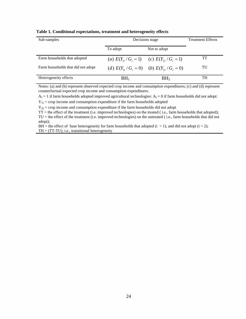
4.4 Conditional expectations, treatment and heterogeneity effects
The aforementioned endogenous switching regression model can be used to compare the
expected crop income and consumption expenditure of the farm households that adopted (a)
with respect to the farm households that did not adopt (b), and to investigate the expected
income and consumption expenditure in the counterfactual hypothetical cases (c) that the
adopted farm households did not adopt, and (d) that the non-adopters farm households adopted.
The conditional expectations for our outcome variables in the four cases are presented in table
1 and defined as follows
iueiii JGYE 11111 )1/( (8a)
iueiii JGYE 22222 )0/( (8b)
equation (4) and the covariates of the welfare outcome equations (5a) and (5b) (Hartman, 1991; Nelson, 1984; and Nawata, 1994).

15
iueiii JGYE 12112 )1/( (8c)
iueiii JGYE 21121 )0/( (8d)
< TABLE 1 ABOUT HERE>
Cases (a) and (b) along the diagonal of table 1 represent the actual expectations
observed in the sample. Cases (c) and (d) represent the counterfactual expected outcomes. In
addition, following Heckman et al. (2001), we calculate the effect of the treatment ‘to adopt’
on the treated (TT) as the difference between (a) and (c)
TTJGYEGYE ueueiiiiii )()()1/()1/( 21121121 (9)
which represents the effect of improved agricultural technology on the crop income and
consumption expenditure of the farm households that actually adopted the technology.
Similarly, we calculate the effect of the treatment of the untreated (TU) for the farm
households that actually did not adopt improved agricultural technologies as the deference
between (d) and (b),
TUJGYEGYE ueueiiiiii )()()0/()0/( 21221221 (10)
We can use the expected outcomes described in (4a)-(4d) to calculate the heterogeneity
effects. For example, farm households that adopted improved technologies may have earned
more income and spend on consumption than farm households that did not adopt regardless of
the fact that they decided to adopt but because of unobservable characteristics such as their
skills. Adapting Carter and Milon (2005) to our case, we define as “the effect of base
heterogeneity” for the group of farm households that decided to adopt as the difference
between (a) and (d),
121121111 )()()0/()1/( BHJJGYEGYE iiueiiiiiii (11)
Similarly for the group of farm households that decided not to adopt, “the effect of base
heterogeneity” is the difference between (c) and (b)
221221222 )()()0/()1/( BHJJGYEGYE iiueiiiiiii (12)
Finally, we investigate the “transitional heterogeneity” (TH), that is if the effect of adopting
improved agricultural technology is larger or smaller for the farm households that actually
adopted the technologies or for the farm household that actually did not adopt in the

16
counterfactual case that they did adopt, that is the difference between equations (9) and (10)
(i.e., (TT) and (TU)).
5. Results and discussion
The data analysis is performed in two steps. In the first section, a description of the
socioeconomic characteristics of the sample households comparing adopters and non-adopters
for both Tanzania and Ethiopia is presented. In the second section, we present the econometric
results on the role of improved chickpea and pigeonpea technology adoption on household
welfare outcomes in rural Ethiopia and Tanzania.
5.1 Descriptive statistics
Table 2 presents the t-test and chi-square comparison of means of selected variables by
adoption status for the surveyed 700 households in Ethiopia and 613 households in Tanzania.
Some of these characteristics are the explanatory variables of the estimated models we present
further on.
The Ethiopian dataset contains 700 farm households and of these, about 32% are
adopters i.e. planted at least one of the improved chickpea varieties during 2006/07 cropping
season. The area planted of improved chickpea varieties is about 0.6 ha for adopters. Average
age of sample household head is about 47 years and about 9% are female-headed. No
significant difference is observable in the age and gender of the household head although the
groups vary in terms of their marital status. Adopter categories do not seem to significantly
vary in terms of primary and junior level of education (1 to 8 years) however adopters have
higher proportion of household heads with secondary education. This suggests that education
might be uncorrelated with decision to adopt. The average active family labor force is 3.7
persons for adopters and 3.4 for non-adopters and the difference is statistically significant
supporting the importance of family labor for adoption of new technologies. The adopter
groups are distinguishable in terms of asset holding whereby adopters own more livestock per
capita, land per capita and farm asset per capita. No significant difference is observable in
access to off-farm activities and practicing water conservation and soil fertility.
Average walking distance to the main market is significantly lower for adopters and
they seem to have also more access to extension service, media service and official positions.
However, there is no significant difference in terms of household membership in different rural
17
institutions. The result also depicts that the adopter categories are distinguishable in terms of
their knowledge of the existing improved chickpea varieties and perception about those
varieties. Adopters have more experience in chickpea farming as well as farmer to farmer seed
exchange. This simple comparison of the two groups of smallholders suggests that adopters
and non-adopters differ significantly in some proxies of physical, human and social capital.
< TABLE 2 ABOUT HERE>
The Tanzanian dataset contains 613 farm households and of these, about 33% are
adopters i.e. planted at least one of the improved pigeonpea varieties during 2006/07 cropping
season. Results show that improved pigeonpea adopter categories are distinguishable in terms
of household characteristics such as household head year of schooling. The level of education
of the household head is significantly higher for improved pigeonpea adopters. No significant
difference is observable in the age of the household head. Similarly, adopter categories are
distinguishable in terms of proxies of asset holding such as non-oxen asset and rented-in land
size perhaps due to farmers who rented in land to reap the benefit by adopting farm technology.
Improved pigeonpea adopters are also distinct in terms of access indicators to extension service
as indicated by number of farmer’s contact with government and non-government extension
agents. Adopters are also more likely to have access to information related with farm
technology, and experience in technology evaluation or transfer. Moreover the adopter
categories tend to vary significantly in terms of their membership in a community or farmer
groups; the share of households with farmer group membership is significantly higher for
pigeonpea adopters.
The adopter groups are also significantly distinguishable in terms of welfare, measured
by livestock income, off-farm income, crop income and consumption per adult equivalent. Off-
farm and crop income per adult equivalent is significantly higher for improved pigeonpea
adopters compared to the non-adopters counterparts. There is also a significant difference in
terms of livestock income per adult equivalent between pigeonpea adopter categories. As far as
crop income and consumption expenditure per adult equivalent is concerned, pigeonpea
adopter categories are distinguishable in crop income while it is not the case for consumption.
In the subsequent part of the chapter, a rigorous analytical model is estimated to verify
whether these differences in mean crop income and consumption per adult equivalent remain
unchanged after controlling for all confounding factors. To measure the impact of adoption, it

18
is necessary to take into account the fact that individuals who adopt improved varieties might
have achieved a higher level of crop income and consumption even if they had not adopted.
5.2 Econometric results
The correlation between adoption of improved farm technology and household welfare
outcomes such as consumption and income is theoretically complex and there are further
empirical pitfalls regarding the impact evaluation problem. We estimated the consumption and
income effect of a superior farming technology based on cross-sectional data available. First
we used propensity score matching fowling by endogenous switching regression model to
address the research questions.
Table 3 report the estimation results for the average treatment effect on the treated
(ATT) of the outcome variable using PSM techniques. In our application of PSM, we first
estimate a probit regression in which the dependent variable equals one if the household
adopted at least one improved technology, zero otherwise. We then check the balancing
properties of the propensity scores. The balancing procedure tests whether or not adopters and
non-adopters observations have the same distribution of propensity scores5. When balancing
test failed, we tried alternative specifications of the probit model; the specification used in this
paper is the most complete and robust specifications that satisfied the balancing tests6. The
quality of the match can be improved by ensuring that matches are formed only when the
distribution of the density of the propensity scores overlaps adopters and non-adopters
observations—that is, when the propensity score densities have “common support.” For this
reason, we used the common support approach for all PSM estimates. For the common support
sample, the probit model was estimated again to obtain a new set of propensity scores to be
used in creating the match. We also retested the balancing properties of the data. All results
presented in the following pages are based on specifications that passed the balancing tests. We
matched adopters and non-adopters observations by two PSM techniques as discussed earlier.
The standard errors of the impact estimates are calculated by bootstrap using 100 replications
for each estimate.
The estimated results based on the two matching algorithms, the Kernel method (KM)
and nearest neighborhood (NNM), are reported in table 3. Our analysis reveals that adoption of 5 A balancing test fails when a t-test rejects the equality of the means of these variables across ranked groupings of the propensity score. 6 Results of balancing test are not reported here but are available on request.

19
improved agricultural technologies has a significant positive impact on crop income although
the impact on consumption expenditure is mixed. For Ethiopia, the overall average gain of
adopting improved chickpea technologies in crop income per adult equivalent ranges from 0.29
to 0.11. The estimated gain was statistically significant at 90% confidence level for NN
matching while it is not significant for KM method. For Tanzania, both KM and NNM
estimates show a positive and statistically significant impact of adoption of improved
pigeonpea technologies on crop income per adult equivalent. Adoption of improved pigeonpea
had raised the crop income by about 98% for NNM and 71% for KM on average compared to
the non-adopters. It is the average difference between crop incomes of similar pairs of the
households belonging to the non-adopters. This indicates that (assuming there is no selection
bias due to unobservable factors) crop income per adult equivalent for farmers who adopted
improved chickpea and pigeonpea varieties is significantly higher than the non adopters.
< TABLE 3 ABOUT HERE>
Results for the casual impact of adoption of improved agricultural technologies on
consumption expenditure are mixed. For Ethiopia, the overall average gain of adopting
improved chickpea technologies in consumption expenditure per adult equivalent ranges from
0.04 for NNM to 0.07 for KM but the result is only significant for the later one. For Tanzania,
adoption of improved pigeonpea technologies had no significance impact on consumption
expenditure per adult equivalent. The PSM results do not show strong evidence concerning the
positive causality between adoption of improved technologies and consumption expenditure.
This perhaps may be because of the consumption behavior of the household that in the short
run farmers may not adjust immediately with income. But also it may be because PSM cannot
provide consistent estimation of causal effects in the presence of hidden bias.
To check the robustness of our PSM findings, we estimated endogenous switching
regression that can control for unobservable selection bias. The full information maximum
likelihood estimates of the endogenous switching regression model are reported in table 4a and
4b for pigeonpea adoption in Tanzania7. The first column presents the estimated coefficients of
selection equation (4) on adopting improved pigeonpea or not whereas the second and third
column presents the consumption expenditure and crop income functions (5a) and (5b) for 7 The full information maximum likelihood estimates of the endogenous switching regression model are not reported for chickpea adoption in Ethiopia and can be available on request. Determinates of consumption expenditure and crop income are also not discussed since it is not the primary objective of the paper.

20
farm households that did and did not adopt improved pigeonpea technology. To analyze the
correlates of crop income and consumption expenditure per adult equivalent, we include a
broad set of explanatory variables including household demographic factors, specific
individual/household head characteristics, asset holdings, district level factors, and policy
related variables. Results from the endogenous switching regression model estimated by full
information maximum likelihood shows that the estimated coefficient of correlation between
the pigeonpea adoption equation and the consumption expenditure function (j ) is negative
and significantly different from zero. The results suggest that both observed and unobserved
factors influence the decision to adopt modern agricultural technology and welfare outcomes
given the adoption decision. The significance of the coefficient of correlation between the
adoption equation and the welfare of adopters indicates that self-selection occurred in the
adoption of improved agricultural technologies. The differences in the consumption
expenditure equation coefficient between the farm households that adopted improved
pigeonpea and that did not illustrate the presence of heterogeneity in the sample (Table 4,
column 2 and 3). The consumption expenditure function of farm households that adopted
improved pigeonpea is significantly different (at the 1 percent level) from the consumption
function of the farm household that did not adopt.
< TABLE 4 ABOUT HERE>
Table 5 presents the expected household welfare outcome (i.e. crop income and
consumption expenditure) under actual and counterfactual conditions for Tanzania. The
predicted crop-incomes and consumption per adult equivalent from endogenous switching
regression model are used to examine the mean crop-incomes and consumption expenditure
gap between adopters and had they not been adopt. Cell (a) and (b) represent the expected crop
income and consumption expenditure per adult equivalent observed in the sample. The
expected crop income per adult equivalent by farm households that adopted is higher than the
group of households that did not adopt. This simple comparison, however, can be misleading
and drive the researcher to conclude that on average the farm households that adopted
improved technology earned more than the farm households that did not adopt.
< TABLE 5 ABOUT HERE>

21
The last column of table 5 presents the treatment effects of adoption of pigeonpea. The
result from the regression indicates that the mean value of crop income per adult equivalent of
pigeonpea adoption is statistically higher than had they not been adopt. This is consistent with
the result from propensity score matching. Improved pigeonpea adoption increases crop-
incomes per adult equivalent by about 109%. For non-adopters the mean crop income per adult
equivalent would have been increased by 44% had they adopted improved pigeonpea.
Unlike to PSM results which compares the treated and control based on observable
variables, the result from switching regression confirms that adoption of pigeonpea have also a
positive impact on consumption expenditure per adult equivalent. It clearly shown that
pigeonpea adopters mean consumption expenditure per adult equivalent is 72% higher. When
non-adopters had adopted improved pigeonpea their consumption per adult-equivalent, would
have been increased by 70%. These results imply that adoption of improved agricultural
technologies increased household welfare measured in terms of crop income and consumption
expenditure, however, the transitional heterogeneity effect for both crop income and
consumption expenditure is positive, that is the effect is bigger for the farm household that did
adopt with respect to those that did not adopt.
6. Conclusions
This paper evaluates the potential impact of adoption of improved chickpea and pigeonpea
technologies on rural household welfare measured by crop income and consumption expenditure in
rural Ethiopia and Tanzania. The study utilizes cross-sectional farm household level data collected in
2007 from a randomly selected sample of 1313 households (700 in Ethiopia and 613 in Tanzania). We
estimate the casual impact of technology adoption by utilizing endogenous switching regression and
propensity score matching methods to assess results robustness. This helps us estimate the true welfare
effect of technology adoption by controlling for the role of selection problem on production and
adoption decisions.
The causal impact estimation from both the propensity score matching and switching
regression suggests the improve pigeonpea adopters have significantly higher crop income than
non-adopters even after controlling for all confounding factors. The results from switching
regression also confirms that adoption pigeonpea has significant impact on consumption
expenditure per adult equivalent although the result from propensity score matching is not
significant suggesting that controlling unobserved heterogeneities are important. for Ethiopia,

22
propensity score matching estimates show that adoption of improved chickpea has a positive
and significant effect on crop income per adult equivalent although the impact on consumption
expenditure is mixed. The results from this paper generally confirms the potential direct role of
agricultural technology adoption on improving rural household welfare, as higher incomes from
improved technology translate into lower income poverty.
References
Alene, A. and Manyong, V.M. (2007). The effect of education on agricultural productivity
under traditional and improved technology in northern Nigeria: an endogenous
switching regression analysis. Empirical Economics 32: 141-159.
Becker, S. O. and Ichino, A. (2002). Estimation of average treatment effect based on
propensity score. Stata Journal 4: 358-77.
Byerlee, D. (2000). Targeting poverty alleviation in priority setting for agricultural research.
Food Policy 25:429–45.
Carter, D.W. and Milon, J.W. (2005). Price knowledge in household demand for utility
services. Land Economics 81(2): 265-283.
Dehejia, H.R., and Wahba, S. (2002). Propensity score matching methods for non-experimental
causal studies. The Review of Economics Statistics 84(1): 151-161.
Freeman, H.A., van der Merwe, P.J.A, Subrahmanyam, P, Chiyembekeza, A.J, and Kaguongo,
W. (2001). Assessing the adoption potential of new groundnut varieties in Malawi.
Working Paper 11, ICRISAT, Patancheru, India.
Hartman, R.S. (1991): A Monte Carlo analysis of alternative estimators in models involving
selectivity. Journal of Business and Economic Statistics 9: 41-49.
Hausman, J.A. (1978). Specification tests in econometrics. Econometrica 46: 1251-1272.
Heckman, J. (1979). Sample selection as a specification error. Econometrica 47: 153–161
Heckman, J., Ichimura, H., Smith, J. and Todd, P. (1998). Characterizing selection bias using
experimental data. Econometrica 66 (5): 1017-1098.
Heckman, J.J., Tobias, J.L. and Vytlacil, E.J. (2001). Four parameters of interest in the
evaluation of social programs. Southern Economic Journal 68(2): 210-233.
Lee, L.F. and Trost, R.P. (1978). Estimation of some limited dependent variable models with
application to housing demand. Journal of Econometrics 8: 357-382.
Lipton M. and Longhurst R. (1989). New seeds and poor people. London: Routledge.

23
Lokshin, M. and Sajaia, Z. (2004). Maximum Likelihood Estimation of Endogenous
Switching Regression Models. Stata Journal 4(3): 282-289.
Maddala, G.S. and Nelson, F.D. (1975). Switching regression models with exogenous and
endogenous switching. Proceeding of the American Statistical Association (Business
and Economics Section), pp. 423-426.
Maddala, G.S. (1983). Limited dependent and qualitative variables in econometrics.
Cambridge, U.K.: Cambridge University Press.
Manyong, V.M., Douthwaite, B., Coulibaly, O., and Keatinge, J.D.H. (2001). Participatory
impact assessment at the International Institute of Tropical Agriculture: functions and
mechanisms. Proceedings of a workshop organized by the Standing Panel on Impact
Assessment, CGIAR, 2001
Nawata, K. (1994). Estimation of sample selection bias models by the maximum likelihood
estimator and Heckman’s two-step estimator. Economics Letters 45: 33-40.
Nelson, F.D. (1984). Efficiency of the two-step estimator for models with endogenous
sample selection. Journal of Econometrics 24: 181-196.
Rosenbaum, P.R., and Rubin, D.B. (1983). The central role of the propensity score in
observational studies for causal effects. Biometrika 70(1): 41-55.
Shiferaw, B. and Teklewold, H. (2007). Structure functioning of chickpea markets: evidence
based on analysis of value chains linking smallholders and markets, Working Paper 6,
International Livestock Research Institute (ILRI), Nairobi, Kenya.
Shiferaw, B., Kebede, T.A. and You, L. (2008). Technology adoption under seed access
constraints and the economic impacts of improved pigeonpea varieties in Tanzania’,
Agricultural Economics 39 (3): 309-323.
Smith, J. and Todd, P. (2005). Does matching overcome LaLonde’s critique of non-
experimental Estimators? Journal of Econometrics 125(1-2): 305-353.
WDR (2008). World development report 2008: agriculture for development, The World
Bank, Washington, DC.
Wooldridge, J.M. (2005). Instrumental estimation of the average treatment effect in the
correlated random coefficient model. Department of Economics, Michigan State
University, Michigan.
24
Table 1. Conditional expectations, treatment and heterogeneity effects
Sub-samples Decisions stage Treatment Effects
To adopt Not to adopt
Farm households that adopted )1/()( 1 ii GYEa )1/()( 2 ii GYEc TT
Farm households that did not adopt )0/()( 1 ii GYEd )0/()( 2 ii GYEb TU
Heterogeneity effects BH1 BH2 TH
Notes: (a) and (b) represent observed expected crop income and consumption expenditures; (c) and (d) represent counterfactual expected crop income and consumption expenditures. Ai = 1 if farm households adopted improved agricultural technologies: Ai = 0 if farm households did not adopt: Y1i = crop income and consumption expenditure if the farm households adopted Y2i = crop income and consumption expenditure if the farm households did not adopt TT = the effect of the treatment (i.e. improved technologies) on the treated ( i.e., farm households that adopted); TU = the effect of the treatment (i.e. improved technologies) on the untreated ( i.e., farm households that did not adopt); BH = the effect of base heterogeneity for farm households that adopted (i = 1), and did not adopt (i = 2); TH = (TT-TU), i.e., transitional heterogeneity

25
Table 2. Descriptive summary of variables used in estimations
Variables
Ethiopia Tanzania
Adopters (N =222 )
Non-adopters
(N = 478 )
t-stat (chi-
square)
Adopters (N =202 )
Non-adopters
(N = 411 )
t-stat (chi-
square)
Dependent variables
Crop income per adult equivalent (‘000 Birr/TSh) 3.29 2.87 1.65* 0.26 0.22 0.91
Consumption expenditure per adult equivalent (‘000 Birr/TSh)
3.18 2.74 3.41*** 0.21 0.19 0.81
Household characteristics variables
Age of the household head (years) 47.6 46.7 0.9 46.2 47.0 -0.73
Gender of household head (male = 1) 0.95 0.92 1.1 0.90 0.88 0.55
Household head education (years) 2.4 1.6 2.61*** 6.40 5.60 2.72**
Active family labour force (adult equivalent -AE) 3.7 3.4 2.6*** 3.60 3.40 1.58
Dependency ratio 1.16 1.09 1.22 0.41 0.42 -0.80
Household wealth variables and farm characteristics
Oxen per AE (number/’000Tsh) 0.55 0.45 3.87*** 12.3 10.0 1.68*
Value of farm asset owned per AE (’000 Birr/Tsh) 0.26 0.16 2.52** 72.6 88.3 0.60
Farm size per AE (ha) 0.42 0.34 3.39*** 0.32 0.34 0.55
Access to off-farm activities (yes = 1) 0.35 0.40 1.49 0.85 0.77 5.39**
Farming main occupation (yes = 1) 0.94 0.94 0.10 0.93 0.94 0.61
Practice soil and water conservation (yes = 1) 0.40 0.40 0.00 0.36 0.46 6.48**
Institutional and access related variables
Contact with government extension agents (number) 28.5 18.4 4.2*** 24.75 13.99 2.91**
Own radio or TV or mobile phone (yes = 1) 0.84 0.75 7.36*** 0.89 0.80 7.53***
Access to credit (1=yes) 0.87 0.81 3.93** 0.08 0.04 4.73**
Member of farmer association (yes = 1) 0.27 0.22 1.6 0.24 0.16 5.97**
Household head hold official position (yes = 1) 0.34 0.25 6.89*** 0.17 0.11 3.44**
Walking distance to main market (km) 12.8 9.3 2.8*** 7.20 7.40 0.49
Distance to extension service (km) 2.5 2.5 -0.08 11.6 12.00 -0.55
Experience of growing chickpea/pigeonpea (years) 22.6 19.3 3.3*** 14.7 14.15 0.57
Farmers perception of improved varieties (ranked above average = 1)
0.83 0.29 179.5*** 2.94 2.69 2.75***
Own donkey for transport (yes = 1) 0.89 0.82 5.31** - - -
Own a cart for transport (yes=1) - - - 0.24 0.13 11.37***
Own bicycle (yes =1) 0.01 0.02 1.27 0.66 0.58 3.15*
Note: Statistical significance at the 99% (***), 95% (**) and 90% (*) confidence levels. T-test and chi-square are used for continuous and categorical variables, respectively.

26
Table 3. Impact of agricultural technology adoption on income and consumption expenditure
using PSM methods
Countries Adopters Non-
adopters
Difference = average treatment effect on the treated (ATT)
t-stat
(a) Dependent variable: Log crop income per adult equivalent unit
Method 1: Nearest neighbour matching
Tanzania 11.59 10.61 0.98 1.68*
Ethiopia 3.35 3.07 0.29 1.74*
Method 2: Kernel matching
Tanzania 11.59 10.88 0.71 1.61*
Ethiopia 3.28 3.17 0.11 0.79
(b) Dependent variable: Log consumption expenditure per adult equivalent unit
Method 1: Nearest neighbour matching
Tanzania 5.16 5.134 0.03 0.24
Ethiopia 3.41 3.38 0.04 0.87
Method 2: Kernel matching
Tanzania 5.18 5.16 0.01 0.12
Ethiopia 3.42 3.35 0.07 1.61*
Note: Statistical significance at the 99% (***), 95% (**) and 90% (*) confidence levels. The number in brackets shows bootstrapped standard errors with 100 replication samples.

27
Table 4a. Full information maximum likelihood estimates of the switching regression model
Dependent variable: pigeonpea adoption and log consumption expenditure per adult equivalent for Tanzania
Variables FIML Endogenous Switching Regression
Adoption (1/0 )
Adoption =1 (adopters)
Adoption=0 (non-adopters)
Age of household head 0.001(0.00) 0.001(0.00) 0.001 (0.00)*** Head education 1-4 years 0.126 (0.25) -0.651 (0.20)*** -0.043 (0.13) Head education 5-8 years 0.375 (0.24) -0.578 (0.19)*** -0.187 (0.13) Head education 9-12 years 0.284(0.35) -0.634 (0.25)** -0.144 (0.21) Head education >12 years -0.234 (0.59) 0.000 (0.48) 0.492 (0.34) Family size in AE 0.018 (0.03) -0.077 (0.02)*** -0.089 (0.01)*** Gender of household head -0.158 (0.20) -0.240 (0.15)* -0.055 (0.11) Land per AE 0.088 (0.16) -0.020 (0.05) 0.109 (0.04)*** Log non-oxen asset per AE -0.088 (0.07) 0.108 (0.04)*** 0.093 (0.03)*** Log oxen per AE -0.008 (0.01) -0.002 (0.01) -0.004 (0.01) Log crop income per AE 0.047 (0.03)* -0.011 (0.02) 0.015 (0.01) Log off-farm income per AE 0.099 (0.04)** 0.042 (0.02)* 0.046 (0.02)** Log livestock income per AE 0.05 (0.03) -0.003 (0.02) 0.027 (0.02) Karatu district (reference) Kondoa district -1.408 (0.43)*** 0.061 (0.27) -0.179 (0.09)* Babati district 0.571 (0.18)*** -0.073 (0.14) -0.397 (0.10)*** Arumeru district 0.844 (0.18)*** -0.118 (0.14) -0.032 (0.11) Total rented in land 0.079 (0.05) Land per AE square -0.019 (0.03) Log of distance to nearest agricultural office -0.182 (0.06)*** Log of distance to the main market -0.096 (0.07) Log of contact with government extension agent 0.163 (0.06)*** Log of contact with non-government extension agent 0.077 (0.05) Practice soil and water conservation -0.106 (0.16) Member of cooperative or community group 0.199 (0.25) Had information related with farm technology 0.332 (0.21) Access to credit 0.464 (0.23)** Access to seed 0.807 (0.19)*** Access to media 0.302 (0.19) Owned ox-cart 0.141 (0.18) Owned bicycle 0.233 (0.15) Access to off-farm -0.416 (0.21)** Predicted value of maize -1.024 (1.12) Constant -0.253 (0.74) 5.394 (0.56)*** 4.412 (0.33)***
ei 0.615 (0.04) 0.717 (0.03)
j -0.372 (0.19)* -0.859 (0.04)***
Notes: absolute value of robust standard error in parenthesis, *Significant at the 10% level, ** significant at 5%, and *** significant at 1% level.

28
Table 4b. Full information maximum likelihood estimates of the switching regression model
Dependent variable: pigeonpea adoption and log crop income per adult equivalent for Tanzania
Variables FIML Endogenous Switching Regression
Adoption (1/0 )
Adoption =1 (adopters)
Adoption=0 (non-adopters)
Age of household head 0.017 (0.17) -0.006 (0.68) 0.0 12 (0.40) Family size in AE -0.072 (0.07) -0.011 (0.04) -0.03 (0.04) Education of household head 0.074 (0.02)*** -0.052 (0.06) 0.002 (0.04) Log oxen per AE 0.004 (0.02) -0.001 (0.03) -0.018 (0.02) Log non-oxen asset per AE 0.055 (0.11) 0.179 (0.10)* 0.114 (0.09) Land per AE 0.025 (0.20) 0.376 (0.13)*** 0.485 (0.14)*** Total area under pigeonpea -0.046 (0.09) 0.114 (0.11) 0.147 (0.10) Total area under maize 0.039 (0.10) -0.173 (0.14) -0.116 (0.11) Log of maize marketed 0.047 (0.03) 0.120 (0.03)*** 0.039 (0.04) Average price of maize 0.001 (0.00)*** 0.004 (0.00)*** 0.007 (0.00)*** Average price of pigeonpea -0.04 (0.04) 0.258 (0.08)*** 0.316 (0.06)*** Farming as primary occupation 0.003 (0.38) -0.021 (0.34) -0.357 (0.74) Access to market information -0.091 (0.15) 0.768 (0.39)* 0.253 (0.26) Access to credit -0.112 (0.28) -0.164 (0.34) 0.234 (0.50) Had information related with farm technology 0.256 (0.25) -0.248 (0.30) -0.191 (0.34) Access to off-farm 0.088 (0.18) -0.10 (0.25) -0.398 (0.27) Access to seed 1.128 (0.22)*** 0.048 (0.33) 0.607 (0.54) Karatu district (reference) Kondoa district -2.737 (1.21)** 0.053 (0.37) -0.26 (0.23) Babati district 0.846 (0.27)*** 0.164 (0.31) -0.726 (0.34)** Arumeru district 1.086 (0.23)*** -0.122 (0.10) -0.021 (0.09) Total rented in land 0.225 (0.13)* Land per AE square -0.043 (0.03) Log of distance to nearest agricultural office -0.348 (0.13)*** Log of distance to the main market 0.004 (0.09) Log of contact with government extension agent 0.208 (0.08)*** Log of contact with non-government extension agent 0.133 (0.06)** Practice soil and water conservation 0.356 (0.40) Member of cooperative or community group 1.032 (0.60)* Age of household head square 0.00 (0.00) Access to media 0.52 (0.40) Owned ox-cart 0.546 (0.33)* Owned bicycle 0.494 (0.32) Predicted value of maize -5.148 (3.77) Constant -6.454 (9.22) 7.975 (3.30)** 7.975 (3.30)**
ei 1.622(0.12) 2.123 (0.08)
j -0.158 (0.22) -0.342 (0.26)*
Notes: absolute value of robust standard error in parenthesis, *Significant at the 10% level, ** significant at 5%, and *** significant at 1% level.

29
Table 5. Average expected crop income and consumption expenditure per adult equivalent for
pigeonpea adopters and non adopters in Tanzania
Sub-samples Decisions stage Treatment Effect
To adopt Not to adopt
a) Log crop income per adult equivalent
Farm households who adopted (a) 11.61 (c) 10.52 1.09(6.7)***
Farm households who did not adopt (d) 11.37 (b) 10.93 -0.44 (3.28)***
Heterogeneity effects BH1= 0.24 BH2= -0.41 TH= 1.53
b) Log consumption expenditure per adult equivalent
Farm households who adopted (a) 5.16 (c) 4.42 0.74(14.9)***
Farm households who did not adopt (d) 4.94 (b) 5.64 -0.70 (19.9)***
Heterogeneity effects BH1= 0.22 BH2= -1.22 TH= 1.44
Note: absolute value of t-statistic in parenthesis, *Significant at the 10% level, ** significant at 5%, and *** significant at 1% level.