1

ISET GOLDEN JUBILEE SYMPOSIUM Indian Society of Earthquake Technology

Department of Earthquake Engineering Building IIT Roorkee, Roorkee

October 20-21, 2012

Paper No. C007

EFFECT OF FOUNDATION SOIL ON STRUCTURAL ECONOMICS OF EARTHQUAKE RESISTANT DESIGN OF RC

BUILDINGS

Nitesh Ahir1 and G.I. Prajapati2 1 Ph.D. Student, Department of Earthquake Engineering,

Indian Institute of Technology Roorkee, Roorkee - 247667, India. E-mail: nitesh.ahir@gmail.com. 2 Professor, Department of Earthquake Engineering,

Indian Institute of Technology Roorkee, Roorkee - 247667, India. E-mail: giprafeq@iitr.ernet.in.

ABSTRACT

For a particular building, the magnitude of lateral loads due to earthquakes will depend on the zone in which the building is located and the type of soil upon which the building is supported. The variation in the design lateral loads due to seismic zone and the type of soil will affect the size of the structural members like beams, columns and foundations, which in turn, will influence the structural cost of the building. Here, the structural cost refers to the cost of the materials that are structural steel and concrete. This excludes other costs such as labour, electrical and water fittings and cost of non - structural members, etc. An attempt has been made to study the structural economics of the building, i.e., the change in the structural cost when a four storied RC Building in the same Zone and with the same geometry is analyzed, designed and detailed for the varying soil types. The analysis of buildings incorporates Soil - Structure Interaction (SSI) effects as per the guidelines given in FEMA - 440. The analysis, design and detailing of structural members and foundations for three RC buildings are carried out. Finally, the quantity of steel and concrete for each building has been computed and structural cost of materials is obtained. The comparison of the structural cost has been done. Keywords: Earthquake Resistant RC Buildings, Soil - Structure Interaction, Structural Economics.

INTRODUCTION The purpose of this study is to draw the attention towards the effects of foundation soil on the structural cost of the buildings. For this purpose, three cases have been considered. These cases consist of a four-storied RC (Reinforced Concrete) building considered in the same zone (zone IV IS 1893 (Part 1) (2002) [9]) and with the same geometry but varying soil types as per [9] viz., Case I: hard soil, Case II: medium

2

soil, and Case III: soft soil. Case I does not include SSI effects as per [9] while other two cases incorporate SSI effects as per FEMA 440 (2005) [4]. IDEALIZATION OF MODELS All four-storied symmetrical RC buildings have four bays of 4.5 m each and equal storey height of 3.2 m each. The foundation is assumed to be located at 1.5 m depth in all cases. All structural members are considered to be made of concrete of grade M 20 and reinforced steel of grade Fe 415. The floor diaphragms are assumed as rigid. Sizes of all columns and all beams are kept same. Slabs have not been modeled. The dead loads, live loads and load combinations for the model are taken as per IS 875 (Part 1) (1987) [6], IS 875 (Part 2) (1987) [7], IS 875 (Part 5) (1987) [8]. More details of load application and model development are given in Ahir, N. (2009) [1]. SOIL-STRUCTURE INTERACTION SSI effects are generally neglected in earthquake resistant design of buildings and this leads to the overestimation of forces resulting into increase in the size of members and hence, the structural cost. There are two effects of SSI: (i) kinematic interaction effects and (ii) inertial interaction. The kinematic interaction effects is due to the difference of Free-Field Motion (FFM) and the ground motion imposed at the foundation of a structure because of averaging of variable ground motions across the foundation slab, wave scattering and embedment effects. The inertial interaction effects cause deformation and stresses in supporting soil and therefore, inertial interaction effects are mainly associated with the modification of dynamic response of structural system. Procedure to Incorporate SSI The procedure to incorporate SSI effects as given in [4] is given below: 1. Kinematic Interaction (KI) Effects

1. Evaluate the effective foundation size be = ,ab where a and b are the full footprint dimensions (in feet) of the building foundation in plan view.

2. Evaluate the Ratio of Response Spectra (RRS) due to base-slab averaging (RRSbsa) as a function of period from Eq. (1).

2.1

1410011

TbRRS e

bsa the value for T = 0.2 s (1)

3. If the structure has a basement embedded depth e from the ground surface, evaluate an additional

RRS due to embedment (RRSe) as a function of period from Eq. (2).

se nT

eRRS2cos the larger of 0.453

or the RRSe value for T = 0.2 s. (2)

where, e = basement embedment (in feet); vs = shear wave velocity for site soil conditions, taken as average value of velocity to a depth of be below foundation (ft/s); n = shear wave velocity

3

reduction factor for the expected Peak Ground Acceleration (PGA) as given in Table 1, where g is the acceleration due to gravity.

4. Evaluate the product of RRSbsa times RRSe to obtain the total RRS for each period of interest. The spectral ordinate of the Foundation Input Motion (FIM) at each period is the product of the FFM spectrum and the total RRS.

5. Repeat steps 2 through 4 for other periods if desired to generate a complete spectrum for the FIM. 2. Inertial Interaction Effects

i. Effective-Dynamic Shear Modulus: The most important parameter required to incorporate SSI effects is stiffness parameter, i.e., effective or dynamic shear modulus of soil. The computation procedure of effective or dynamic shear modulus, G, is given in subsequent steps. 1. The type of site for SSI analysis as per [4] has been identified by comparing the types of soil

constituting the foundation as per [9], IS 2131 (1981) [10] and Table 2 taken from ATC 40 [2]. For present study, site class D and site class E of [4] are taken for Case II and Case III, respectively.

2. The value of short-period response acceleration parameter for site class B [4], SS, are determined from UFC 3-310-01 (2007) [13] obtained for 2500 years event.

3. The maximum considered short-period spectral response acceleration parameter, SXS = Fa SS, where, Fa is site coefficient determined from Table 3, based on the site class and the value of the response acceleration parameter, SS.

4. Five - percent damped design spectral response acceleration at short periods, SDS = 2 SXS / 3. 5. The initial shear modulus, Go = γ (vs)2/g , where vs is the shear wave velocity at low strains, γ

is the weight density of the soil, and g is the acceleration due to gravity. 6. The effective-dynamic shear modulus, G, shall be calculated in accordance with values of

ratio of effective shear modulus given in tabulated form in FEMA 356 [3].

ii. Soil-Stiffness Factors: Using the soil-stiffness factors given in [3], the stiffness terms can be calculated for embedded foundations.

iii. System Damping

1. Evaluate the linear periods for the structural model assuming a fixed base, T, and a flexible base, T , using appropriate foundation modeling assumptions.

2. Calculate the effective structural stiffness of the single degree of freedom (SDOF) oscillator for fixed base conditions from Eq. (3). In Eq. (3), M* is the effective mass for the first mode calculated as the total mass times the effective mass coefficient, m , which is calculated from Eq. (4). In Eq. (4), wi is weight assigned to level i, im is amplitude of mode m at level i, N is level N, the level which is uppermost in the main portion of the structure, g is acceleration due to gravity.

2

** 2

TMK fixed

(3)

4

gwgw

gw

N

imi

N

ii

N

imi

m

1

2

1

2

1

(Unit-less) (4)

3. Determine the equivalent foundation radius for translation, rx, from Eq. (5). In Eq. (5), Af is the area of the foundation footprint if the foundation components are inter-connected laterally.

fx

Ar (5)

4. Calculate the translational stiffness of the foundation, Kx = 8 G rx / (2 – υ), where, G is effective strain - degraded soil shear modulus and υ is soil Poisson’s ratio.

5. Calculate the equivalent foundation radius for rotation, rθ, by first evaluating the effective rotational stiffness of the foundation, Kθ, from Eq. (6). In Eq. (6), h* is the effective structure height taken as the full height of the building for one-story structures and as the vertical distance from the foundation to the centroid of the first mode shape for multi-story structures. In the latter case, h* can often be well approximated as 70 % of the total structure height. The quantity Kx is often much larger than K*

fixed, in which case an accurate evaluation of Kx is unnecessary and the ratio, K*

fixed/Kx, can be approximated as zero. The equivalent foundation radius for rotation is then calculated from Eq. (7). In Eq. (7), soil shear modulus, G, and soil Poisson’s ratio, υ, should be consistent with those used in the evaluation of foundation spring stiffness.

x

fixed

fixed

KK

TT

hKK

*2~

2**

1

)(

(6)

31

3)1(3

G

Kr

(7)

6. Determine the basement embedment, e, if applicable. 7. Estimate the effective period-lengthening ratio, ,effeff TT using the site-specific structural

model developed for nonlinear pushover analysis. This period-lengthening ratio is calculated for the structure in its degraded state (i.e., accounting for structural ductility and soil ductility). An expression for the ratio is given by Eq. (8). In Eq. (8), the term μ is the expected ductility demand for the system (i.e., including structure and soil effects).

5

5.02

111

TT

TT

eff

eff

(8)

8. Evaluate the initial fixed-base damping ratio for the structure, βi, which is often taken as 5

%. 9. Determine foundation damping due to radiation damping, βf, from Eq. (9). Eq. (9) is

applicable for effeff TT < 1.5, and generally provide conservative (low) damping estimates

for higher effeff TT .

2

21 11

eff

eff

eff

efff T

TaTTa % (9)

where, a1 = ce exp (4.7 −1.6h / rθ ), a2 = ce [25 ln (h/rθ) – 16] and ce = 1.5 (e / rx ) + 1 10. Evaluate the flexible-base damping ratio,β0, from Eq. (10).

3effeff

ifo

TT

(10)

11. Evaluate the effect on spectral ordinates for the change in damping ratio from βi to β0, then modify the spectrum of the foundation input motion.

MODELING, ANALYSIS AND DESIGN The modeling, analysis and design of buildings for considered three cases have been described in detail in [1]. The kinematic interaction effects have been neglected for Case III as per [4]. The sample calculations for illustration of incorporation of kinematic interaction effects for Case II are shown in Table 4. The calculation of values of effective-dynamic shear modulus for Case II and Case III are shown in Table 5. With the help of soil stiffness factors given in tabulated form in [3], the soil-stiffness factors determined for Case II and Case III are given in Table 6 and Table 7, respectively. The dimension of isolated-square footing is assumed as 2.4 m x 2.4 m x 0.6 m for the determination of soil-stiffness factors for both Case II and Case III. The assumed dimension and type of footing for Case II are found to be compatible with the designed foundation type. For Case III, the bearing capacity of the soil is low, and therefore, the raft foundation has to be provided in place of isolated footings. Therefore, the raft foundation of size 20 m x 20 m x 0.5 m was made to evaluate soil stiffness factors for whole mat area. Table 7 gives two values of stiffness factors; they are for Case III for whole mat-foundation area and for 4.5m x 4.5m area. In SAP [12], the mat foundation can be modeled by using an area element. The stiffness factors for a mat foundation can be applied as area springs by dividing the mat area into some number of elements (see in [12], help>mat>area springs). Therefore, the whole mat area is divided into sixteen numbers of elements, which are equal to the number of slabs at any level. Then, the stiffness factors are divided by sixteen and the stiffness factors are entered in [12] for the area equal to that of a slab, i.e., 4.5m x 4.5m = 20.25 m2 and this value of area has also been entered in [12]. The values of flexible base damping for Case II and Case III calculated according to the procedure discussed in the preceding section are shown in Table 8. The summary of the analysis performed in [12] is given in Table 9.

In Table 9, the base shear ratio BB VV_

represents ratio of design base shear obtained using fundamental time period of the structure to the base shear obtained from response spectrum analysis in [12]. Sa/g and

6

Tn are the average response acceleration coefficient and the natural or fundamental time period of the structure obtained as per [9], respectively. Scale factor (SF = ZIg/2R), which is analogous to design horizontal seismic coefficient defined in [9], when SF and response spectrum are together considered in analysis in [12]. According to [9], when base shear obtained from response spectrum method is less than the base shear obtained using fundamental time period of the structure, all the response quantities like member forces, displacements, storey forces, storey shears and base reactions are multiplied by base shear ratio. This multiplication of base shear ratio is apparently done in [12] by modification of SF. The design and detailing of buildings are performed as per IS 456 (2000) [5], IS 13920 (1993) [11].

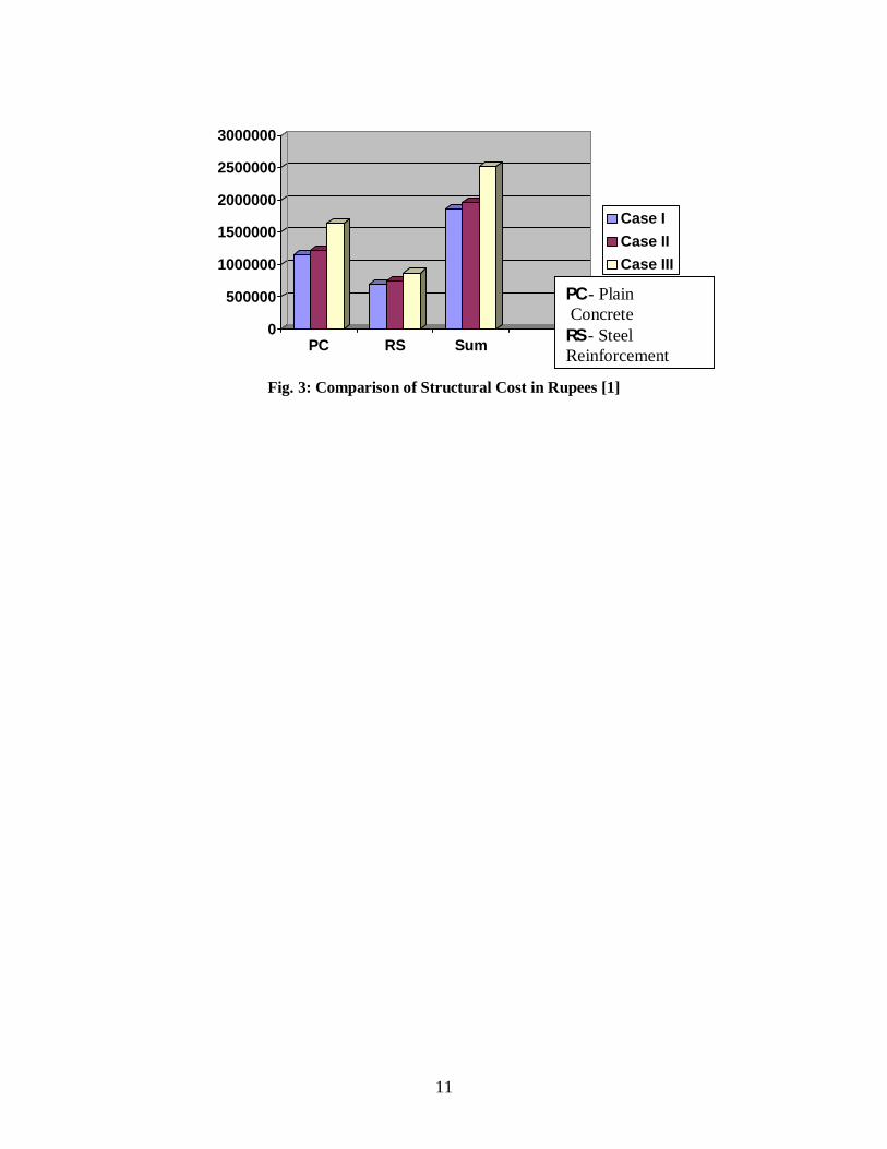
RESULTS AND CONCLUSION The comparison of structural cost, in terms of cost of required quantity of plain concrete in beams, columns and footings for all the considered cases, is shown in Figure 1. The comparison of structural cost, in terms of cost of required quantity of reinforced steel in beams, columns and footings for all the considered cases, is shown in Figure 2. The comparison of structural cost for all considered cases is shown in Figure 3. The following conclusions are drawn from the comparison of structural cost among the considered three cases:

1. The cost of concrete required for Case II and Case III increased by 5 % and 42 %, respectively, in comparison to Case I.

2. The cost of reinforced steel required for Case II and Case III increased by 6 % and 25 %, respectively, in comparison to Case I.

3. The structural cost for Case II and Case III increased by 6 % and 36 %, respectively, in comparison to Case I.

The following SSI effects have been observed during the analysis for Case II and Case III as deciphered from Table 9.

1. The design base shear for Case II considering the fixed base is, 1118.79 kN while the design base shear obtained considering SSI effects comes out to be 1114.07 kN. The fundamental time-period for case II for the fixed base and the flexible base model are, respectively, 1.0605 sec and 1.081 sec. The system damping ratio for Case II has been found as 5.14 %.

2. The design base shear for case III considering the fixed base is, 1118.79 kN while the design base shear obtained considering SSI effects comes out to be 1091.114 kN. The fundamental time-period for case II for the fixed base and the flexible base model are, respectively, 1.0605 sec and 1.1568 sec. The system damping ratio for Case III has been found as 5.81 %.

3. The less variation in the time period obtained from analysis before and after considering SSI in buildings in present study is found to be dependent to some extent upon constant region of response spectrum, as there is no variation in value of average response acceleration coefficient and thus the value of design base shear remained constant for all cases. This approximately equalizes the final base shear of the buildings for all cases. Thus, there is also no variation in time period when the KI was considered and the base was fixed. The little variation in the time period is found to be contributed by the only consideration of inertial interaction in considered cases.

REFERENCES

1. Ahir, N. (2009). ‘Effect of Foundation Soil on Structural Economics of Earthquake Resistance Design

of RC Building’, M. Tech. Dissertation, Department of Earthquake Engineering, Indian Institute of Technology Roorkee - 247667, Roorkee, India.

2. ATC-40 (1996). ‘Seismic Evaluation and Retrofit of Concrete Buildings’, Applied Technology Council, Redwood City, California.

7

3. FEMA 356 (2000). ‘Prestandard and Commentary for the Seismic Rehabilitation of Buildings’, Federal Emergency Management Agency, Washington, D.C.

4. FEMA 440 (2005). ‘Improvement of Nonlinear Static Seismic Analysis Procedures’, Federal Emergency Management Agency, Washington, D.C.

5. IS 456 : 2000 (fourth revision). ‘Indian Standard Plane and Reinforced Concrete Code of Practice’, Bureau of Indian Standards, New Delhi.

6. IS 875 (Part 1) : 1987 (Second revision). ‘Indian Standard Code of Practice for Design Loads (Other than Earthquake) for Buildings and Structures (Dead Loads)’, Bureau of Indian Standards, New Delhi.

7. IS 875 (Part 2) : 1987 (Second revision). ‘Indian Standard Code of Practice for Design Loads (Other than Earthquake) for Buildings and Structures (Imposed Loads)’, Bureau of Indian Standards, New Delhi.

8. IS 875 (Part 5) : 1987 (Second revision). ‘Indian Standard Code of Practice for Special Loads and Load Combination for Buildings and Structures’, Bureau of Indian Standards, New Delhi.

9. IS 1893 (Part 1) : 2002 (fifth revision). ‘Indian Standard Criteria for Earthquake Resistant Design of Structure’, Bureau of Indian Standards, New Delhi.

10. IS 2131 : 1981 (First revision). ‘Indian Standard Method for Standard Penetration Test for Soils’, Bureau of Indian Standards, New Delhi.

11. IS 13920 : 1993 (Reaffirmed 2003). ‘Indian Standard Code of Practice for Ductile Detailing of Reinforced Concrete Structures Subjected to Seismic Forces’, Bureau of Indian standards, New Delhi.

12. SAP 2000 Advanced 10.0.1 ‘Software’ Computers and Structures Inc. University Avenue Berkeley, California, USA.

13. UFC 3-310-01 (2005, Including Change, 2007). ‘Structural Load Data’, United Facilities Criteria, Department of Defense, USA.

Table 1: Approximated Values of Shear Wave Velocity Reduction Factor, n [4] PGA 0.1g 0.15g 0.20g 0.30g n 0.90 0.80 0.70 0.65

Table 2: Typical Shallow Bearing Soil Material Properties [2] Average Properties in Zone of Influence

Soil Profile Type

Description Shear wave Velocity, s

(ft/sec)

SPT N (blows/ft)

Weight Density,

(pcf)

Range of Initial Shear Modulus, Go (psf x 106)

Low High SA Hard Soil > 5000 120 SB Rock 2500 - 5000 140 + 25 120 Sc Dense Soil Soft

Rock 1200 - 2500 > 50 120 - 140 5 25

SD Stiff Soil 600 - 1200 15 – 50 100 – 130 1 5 SE Soft Soil < 600 < 15 90 - 120 < 1

Table 3: Values of Site Coefficient Fa [3]

Site Class

Mapped Spectral Response Acceleration at Short Periods, SS

Ss < 0.25 Ss = 0.50 Ss = 0.75 Ss = 1.00 Ss > 1.25 A 0.8 0.8 0.8 0.8 0.8 B 1.0 1.0 1.0 1.0 1.0 C 1.2 1.2 1.1 1.0 1.0

8

D 1.6 1.4 1.2 1.1 1.0 E 2.5 1.7 1.2 0.9 0.9 F Note b Note b Note b Note b Note b

Table 4: Sample Calculations to Illustrate Incorporation of Kinematic Interaction for Case II [1]

Quantity T (Sa/g)FFM a b be RRSbsa e RRSe (Sa/g)FIM Units sec ft ft ft ft 0 1 59.06 59.06 59.06 0.93 0 1 0.93 0.01 1.15 59.06 59.06 59.06 0.93 0 1 1.07

Table 5: Calculation of Effective Dynamic Shear Modulus [1] Parameters Case II Case III

SS 1.289 1.289 Fa 1 0.9 SDS 0.8593 0.7734 (g/cm3) 1.65 1.6 s (m/s) 150 110 Go (x 106 N/m2) 37.125 19.36 G/Go 0.575 0.215 G (x 106 N/m2) 21.35 4.16

Table 6: Soil Stiffness Factors for Case II [1] Degree of Freedom Units Ksur

(x 108) Kemb

(x 108) Translation along x-axis N/m 1.46 2.24 3.27 Translation along y-axis N/m 1.46 2.24 3.27 Translation along z-axis N/m 1.99 1.37 2.72 Rocking about x-axis N-m/rad 2.44 2.00 4.88 Rocking about y-axis N-m/rad 2.46 2.19 5.39 Rocking about z-axis N-m/rad 3.04 2..49 7.58

Table 7: Soil Stiffness Factors for Case III [1] Degree of Freedom Units Ksu(x108) Kemb (x 108)

For Whole Mat Area For 4.5 m x 4.5 m Area

Translation along x-axis N/m 2.47 1.23 3.03 0.19 Translation along y-axis N/m 2.47 1.23 3.03 0.19 Translation along z-axis N/m 3.56 1.06 3.77 0.24 Rocking about x-axis N-m/rad 30.27 1.07 32.28 2.02 Rocking about y-axis N-m/rad 30.51 1.74 53.00 3.31 Rocking about z-axis N-m/rad 34.63 1.19 41.14 2.57

9

Table 8: Computation of Flexible Base Damping Ratio, β0 [1]

Quantity Units Values Case II Case III T , T sec 1.06, 1.081 1.06, 1.157

m 0.91 0.91

M* kg 1508237.1 1508237.1 K*

fixed N/m 53035560 53035560 Af m2 324 400 rx m 10.15 11.28 G MPa 21.35 4.16 0.4 0.45 Kx N/m 1.084E+09 242364929 h, h* m 12.8, 9.55 12.8, 9.55

K N-m/rad 5.66E+11 1.762E+11

r m 18.14 20.59

, effeff TT 3, 1.01 3, 1.03

e m 0 0 ce, a1, a2 1, 35.55, -24.71 1, 40.67, -27.89

f , i , o % 0.24, 5, 5.14 1.25, 5, 5.81

Table 9: Summary of Analysis Performed in SAP [12]

Case Model No.

Base Type

KI

Tn (sec)

Sa/g BV

_

(kN)

T (sec)

T (sec) BB VV

_

SF

o , %

I 1 Fixed No 0.303 2.5 1118.79 1.061 - 4.037 0.2354 5 2 Fixed No 0.303 2.5 1118.79 1.061 - 0.999 0.9505 5

II 1 Fixed Yes 0.303 2.5 1118.79 1.061 - 3.890 0.2354 5 2 Fixed Yes 0.303 2.5 1118.79 1.061 - 0.780 0.9160 5

10

3 Flexible Yes 0.303 2.5 1118.79 - 1.081 3.030 0.2354 5 4 Flexible Yes 0.303 2.5 1118.79 - 1.081 1.004 0.7135 5.14

III 1 Fixed No 0.303 2.5 1118.79 1.061 - 3.030 0.2354 5 2 Fixed No 0.303 2.5 1118.79 1.061 - 1.000 0.7139 5 3 Flexible No 0.303 2.5 1118.79 - 1.157 2.900 0.2354 5 4 Flexible No 0.303 2.5 1118.79 - 1.157 1.025 0.6828 5.81

0200000400000600000800000

10000001200000140000016000001800000

B C F Sum

Case ICase IICase III

Fig. 1: Comparison of Cost in Rupees of Required Quantity of Plain Concrete [1]

0100000200000300000400000500000600000700000800000900000

B C F Sum

Case ICase IICase III

Fig. 2: Comparison of Cost in Rupees of Required Quantity of Reinforced Steel [1]

B - Beams C - Columns F - Footings

B - Beams C - Columns F - Footings

11

0

500000

1000000

1500000

2000000

2500000

3000000

PC RS Sum

Case ICase IICase III

Fig. 3: Comparison of Structural Cost in Rupees [1]

PC - Plain Concrete RS - Steel Reinforcement