ahs report georgia tech 2006 - vertical flight society

23rd Annual Student Design Competition

Graduate Category

DDaanniieell GGuuggggeennhheeiimm SScchhooooll ooff AAeerroossppaaccee EEnnggiinneeeerriinngg GGeeoorrggiiaa IInnssttiittuuttee ooff TTeecchhnnoollooggyy AAttllaannttaa,, GGeeoorrggiiaa 3300333322

RRaammbblleerr

i

RRaammbblleerr

Acknowledgements We would like to recognize and thank the following individuals for their special assistance in the

completion of this design project:

Dr. Daniel Schrage Dr. Robert Loewy Dr. JVR Prasad

Dr. Dimitri Mavris Dr. Jimmy Tai Dr. Sandeep Agarwal

Dr. Lakshmi Sankar Dr. Amar Atre Dr. Byung-Ho Ahn

Dr. Jou-Young Choi Dr. Vitali Volovoi Dr. David Eames

Dr. Eric N. Johnson Dr. Mark Costello Dr. Ilkay Yavrucuk

Dr. Suresh Kannan Mr. Chang Chen Mr. Russell Denney

Mr. Ian Stults Mr. Blake Moore Mr. Peter Hart

Mr. Patrick Biltgen Mr. Han Gil Chae Mr. Adeel Khalid

Mr. M. Emre Gündüz Ms. Jieun Ku Mr. William Briley

Mr. Roy Smolky Mr. Todd Grossaint CPT Andrew Bellocchio

Mr. Tom Hanson Mr. Alex Moodie Mr. Ludvic Baquie

2006 Georgia Tech Graduate Design Team _____________________________ ____________________________ Matthias Hoepfer (PhD Student) Bernard Laurendeau (Masters Student) _____________________________ ____________________________ Sumit Mishra (PhD Student) Kshitij Shrotri (PhD Student) _____________________________ ____________________________ Apinut Sirirojvisuth (Masters Student) CPT Stephen Suhr (Masters Student) _____________________________ ____________________________ Tobias Theel (Masters Student) Lan Wu (PhD Student) _____________________________ Jaesuk Yang (PhD Student)

ii

RRaammbblleerr

Executive Summary

For a two-place turbine training helicopter to successfully enter today’s challenging market, it

must offer superior performance, handling qualities, and safety capability at a price competitive with that

of the Robinson R-22, the current world sales leader in two-place piston training helicopters. In order to

meet this formidable design challenge, the priority of this design effort was focused on the simplification

of systems and subsystems for both the vehicle and the process by which it would be built. Therefore, an

Integrated Product and Process Development (IPPD) methodology was used to drive the design solution.

For product development, the approach was centered on the heart or “core” of the helicopter – the

main rotor system and the subsystems that make it function properly. As Tom Hanson describes in his

Hub Design Handbook1, these subsystems can be classified as force transmittal, torque generation, and

rotor control. Force transmittal allows the helicopter to effectively harness the lift and moments

generated by the main rotor. Torque generation drives the main rotor by converting the work of the

engine into the torque required for flight. Rotor control enables pilot inputs to be transmitted to the

rotating rotor blades. Only through the simplification and efficient integration of these “core” elements

could a successful design solution be achieved.

This training helicopter was developed out of a commitment to these fundamental design

considerations. The Rambler incorporates an “Ideal Rotor,” based on the Hanson elastic articulated (EA)

rotor system, a new turboshaft engine and compact split-torque transmission, and a simplified flight

control system – the integration of which achieves a synergistic effect in optimizing the vehicle’s “core.”

The “Ideal Rotor” and split-torque transmission provide cost and safety enhancements through parts

reduction and structural redundancy. Exceptional handling qualities can also be attributed to this rotor

system design. The new turboshaft engine utilizes a simplified design approach to significantly improve

its overall reliability, performance, and cost in comparison to existing turbine and piston alternatives. The

simplified flight control system eliminates the need for hydraulic actuators, force-feel systems, or

augmentation, except for the yaw axis – thus reducing the weight and complexity of this subsystem.

For process development, a Product Lifecycle Management (PLM) approach was used –

capitalizing on the capabilities of state-of-the-art manufacturing analysis tools. By creating an integrated

computer aided design and manufacturing (CAD-CAM) environment, the processes and resources

required to produce the vehicle are optimized using virtual scenarios – thus improving the overall

efficiency, quality, and cost of production.

Ultimately, the implementation of this IPPD methodology resulted in the development of a

vehicle system solution that is far superior in performance, handling qualities, and safety to any training

helicopter currently on the market.

iii

RRaammbblleerr

Table of Contents

ACKNOWLEDGEMENTS ....................................................................................................................... I EXECUTIVE SUMMARY ....................................................................................................................... II TABLE OF CONTENTS ........................................................................................................................ III LIST OF FIGURES ..................................................................................................................................VI LIST OF TABLES ................................................................................................................................ VIII LIST OF SYMBOLS AND ABBREVIATIONS ....................................................................................IX PROPOSAL REQUIREMENTS MATRIX ......................................................................................... XII TABLE OF PHYSICAL DATA................................................................................................................. 1 DIAGRAM SHEET 1 - THREE-VIEW DIAGRAM............................................................................... 2 DIAGRAM SHEET 2 - AIRCRAFT PROFILE ...................................................................................... 3 DIAGRAM SHEET 3 – ENGINE CENTERLINE SCHEMATIC......................................................... 4 DIAGRAM SHEET 4 – DRIVE TRAIN SCHEMATIC ......................................................................... 5 1 INTRODUCTION.................................................................................................................................... 6 2 REQUIREMENTS ANALYSIS.............................................................................................................. 7

2.1 TRAINING HELICOPTER MISSION ANALYSIS ....................................................................................... 7 2.2 TRAINING HELICOPTER MARKET RESEARCH...................................................................................... 9 2.3 OVERALL DESIGN APPROACH TRADE STUDY ................................................................................... 10

3 PRELIMINARY VEHICLE SIZING AND PERFORMANCE ........................................................ 10 3.1 VEHICLE CONFIGURATION SELECTION ............................................................................................. 10

3.1.1 Vehicle Sizing Methodology ...................................................................................................... 10 3.2 VEHICLE PERFORMANCE ................................................................................................................... 13

3.2.1 Aircraft Drag Estimation ............................................................................................................ 13 3.2.2 Height-Velocity Diagram ........................................................................................................... 14 3.2.3 Vehicle Performance Charts ....................................................................................................... 14

3.3 VEHICLE WEIGHT AND BALANCE...................................................................................................... 16 3.3.1 Component Weight Analysis ...................................................................................................... 16 3.3.2 Center of Gravity Envelope Estimation...................................................................................... 17

4 MAIN ROTOR AND HUB DESIGN ................................................................................................... 18 4.1 HUB SELECTION TRADE STUDY ........................................................................................................ 18 4.2 MAIN ROTOR BLADE DESIGN............................................................................................................ 20

4.2.1 Airfoil Selection.......................................................................................................................... 20 4.2.2 Blade Twist................................................................................................................................. 21 4.2.3 Material Selection....................................................................................................................... 21 4.2.4 Blade Section Properties............................................................................................................. 22 4.2.5 Fatigue Life Estimation .............................................................................................................. 22 4.2.6 Manufacturing............................................................................................................................. 23

4.4 HANSON “IDEAL ROTOR” HUB ANALYSIS ........................................................................................ 23 4.4.1 Modeling Methodology .............................................................................................................. 23 4.4.2 Flexure Design............................................................................................................................ 24

iv

RRaammbblleerr

4.4.3 Static Droop Analysis ................................................................................................................. 26 4.4.4 Quasi-Static Analysis.................................................................................................................. 26 4.4.5 Auto-Trim Validation ................................................................................................................. 27 4.4.6 Ground Resonance...................................................................................................................... 28 4.4.7 Air Resonance............................................................................................................................. 29 4.4.8 Rotor Noise Considerations ........................................................................................................ 30

5 TAIL ROTOR AND EMPENNAGE DESIGN ................................................................................... 30 5.1 CONFIGURATION TRADE STUDY ....................................................................................................... 30 5.2 TAIL ROTOR SIZING........................................................................................................................... 31 5.3 VERTICAL FIN.................................................................................................................................... 31 5.4 HORIZONTAL STABILIZER.................................................................................................................. 31 5.5 EMPENNAGE ...................................................................................................................................... 32

6 PROPULSION SYSTEM DESIGN...................................................................................................... 32 6.1 DESIGN SCOPE ................................................................................................................................... 32 6.2 PARAMETRIC CYCLE ANALYSIS ........................................................................................................ 33

6.2.1 Turbine Cooling Trade Study ..................................................................................................... 35 6.2.2 Parametric Cycle Analysis Conclusions ..................................................................................... 36

6.3 PERFORMANCE CYCLE ANALYSIS ..................................................................................................... 36 6.3.1 Component Performance Maps .................................................................................................. 37

6.4 COMPONENT DESIGN CONSIDERATIONS ........................................................................................... 37 6.4.1 Compressor Configuration Selection.......................................................................................... 37 6.4.2 Centrifugal Compressor Design.................................................................................................. 38 6.4.3 Turbine Section Design .............................................................................................................. 39 6.4.4 Combustion Section Design........................................................................................................ 41 6.4.5 Modular Gearbox Design ........................................................................................................... 41

6.5 SPECIFICATIONS AND PERFORMANCE ANALYSIS .............................................................................. 42 6.6 WEIGHT ANALYSIS ............................................................................................................................ 43 6.7 MANUFACTURING.............................................................................................................................. 43 6.8 FEDERAL AVIATION REGULATIONS (FAR) REQUIREMENTS............................................................. 44 6.9 ADDITIONAL ENGINE DESIGN CONSIDERATIONS .............................................................................. 45

6.9.1 Control System ........................................................................................................................... 45 6.9.2 Air Filtration System .................................................................................................................. 45

6.10 TRANSMISSION DESIGN ................................................................................................................... 46 6.10.1 Configuration Selection ............................................................................................................ 46 6.10.2 Sizing and Analysis .................................................................................................................. 47 6.10.3 Auxiliary Gearbox .................................................................................................................... 49

7 STRUCTURAL DESIGN...................................................................................................................... 50 7.1 STRUCTURAL DESIGN CRITERIA........................................................................................................ 50 7.2 FUSELAGE DESIGN............................................................................................................................. 50

7.2.1 Configuration Selection .............................................................................................................. 50 7.2.2 Composite Structure ................................................................................................................... 51 7.2.3 Manufacturing............................................................................................................................. 52

7.3 LANDING GEAR ................................................................................................................................. 53 7.3.1 Configuration Selection .............................................................................................................. 53 7.3.2 Dimensions and Materials .......................................................................................................... 53 7.3.3 Crashworthiness Analysis........................................................................................................... 53 7.3.4 Landing Gear Dampers............................................................................................................... 55

v

RRaammbblleerr

8 STABILITY AND CONTROL ANALYSIS........................................................................................ 56 8.1 FLIGHT CONTROLS LAYOUT.............................................................................................................. 56 8.2 FLIGHT CHARACTERISTICS ................................................................................................................ 56

8.2.1 Helicopter Trim Solutions .......................................................................................................... 56 8.2.2 Linear Control Root Locus Plots ................................................................................................ 59 8.2.3 FlightLab Modeling .................................................................................................................... 61

8.3 HANDLING QUALITIES....................................................................................................................... 63 8.4 FEDERAL AVIATION REGULATIONS (FAR) REQUIREMENTS............................................................. 65 8.5 GEORGIA TECH UNIFIED SIMULATION TOOL (GUST) ...................................................................... 65

9 COCKPIT LAYOUT DESIGN............................................................................................................. 66 9.1 HUMAN SIZE AND VISIBILITY CONSIDERATIONS .............................................................................. 66 9.2 AIR CREW SEAT DESIGN ................................................................................................................... 67 9.3 CONSOLE CONFIGURATION ............................................................................................................... 67

10 MANUFACTURING AND COST ANALYSIS ................................................................................ 68 10.1 PRODUCT LIFECYCLE MANAGEMENT (PLM).................................................................................. 68

10.1.1 Virtual Engine Gearbox Assembly ........................................................................................... 69 10.2 COST ANALYSIS............................................................................................................................... 69

10.2.1 Engine Cost Model ................................................................................................................... 69 10.2.2 Recurring Cost .......................................................................................................................... 70 10.2.3 Direct Operating Cost (DOC) ................................................................................................... 71 10.2.4 Indirect Operating Cost............................................................................................................. 72

11 SAFETY ANALYSIS AND AIRCRAFT CERTIFICATION ......................................................... 72 11.1 SAFETY ANALYSIS........................................................................................................................... 72

11.1.1 Functional Analysis .................................................................................................................. 72 11.1.2 Functional Hazard Assessment................................................................................................. 73 11.1.3 Preliminary System Safety Assessment (PSSA)....................................................................... 73

11.2 CERTIFICATION PLAN ...................................................................................................................... 74 12 CONCLUSION .................................................................................................................................... 75 APPENDIX A..........................................................................................................................................A-1 APPENDIX B .......................................................................................................................................... B-1

APPENDIX C..........................................................................................................................................C-1

REFERENCES...................................................................................................................................REF-1

vi

RRaammbblleerr

List of Figures

Figure 1: Georgia Tech Preliminary Design Product and Process Development 6 Figure 2: Typical Mission Profile for Initial Rotary Wing Training (VFR Flight) 8 Figure 3: Typical Mission Profile for Advanced Rotary Wing Training (IFR Flight) 8 Figure 4: Rf Methodology 11 Figure 5: Rf Iteration Loop 11 Figure 6: Historical Weight Comparison 13 Figure 7: Height-Velocity Diagram Comarison 14 Figure 8: Rambler Performance Summary (SLS) 14 Figure 9: HOGE Altitude vs. Gross Weight 15 Figure 10: Payload vs. Range 15 Figure 11: Altitude vs. Maximum Continuous Speed 15 Figure 12: Weight and Balance Reference Lines 16 Figure 13: Estimated Center-of-Gravity Envelope 18 Figure 14: Hanson Hub Design 18 Figure 15: Steep Scale Pareto Chart 19 Figure 16: Conservative Scale Pareto Chart 19 Figure 17: Airfoil Power Requirements 20 Figure 18: Airfoil Rate of Climb Capability 20 Figure 19: Main Rotor Blade Cross-Section 21 Figure 20: Main Rotor Airfoil Mesh in ANSYS 22 Figure 21: Goodman Diagram for Kevlar 49/Epoxy 22 Figure 22: Goodman Diagram for S Glass/Epoxy 22 Figure 23: Simplified DYMORE Hub Model 24 Figure 24: Detailed DYMORE Hub Model 24 Figure 25: Standard Flexure Cross Section 24 Figure 26: Flexure Dimensions 25 Figure 27: Main Rotor Static Droop 26 Figure 28: Hanson Hub Fan Plot 27 Figure 29: Hanson Hub Feathering Auto-Trim 28 Figure 30: Ground Resonance Model 28 Figure 31: Ground Resonance Plot 29 Figure 32: Air Resonance Equations 29 Figure 33: Current Industry Trends for Key Turbine-Engine Design Parameters 33 Figure 34: "On-Design" Point Parametric Analysis 35 Figure 35: Turbine Cooling Technology Assessment 36 Figure 36: Turbine Cooling Trade Study 36 Figure 37: NEPP Engine Model 36 Figure 38: Centrifugal Compressor Performance Map 38 Figure 39: Blade Stress vs. Specific Strength 40 Figure 40: Turbine Material Selection Plot 40 Figure 41: High Pressure Turbine Performance Map 40 Figure 42: Power Turbine Performance Map 40 Figure 43: HP Available vs. Altitude (ISA) 42 Figure 44: HP Available vs. Altitude (ISA+20oC) 42 Figure 45: Fuel Flow vs. Altitude (TOP) 42 Figure 46: Fuel Flow vs. Altitude (MCP) 42 Figure 47: SFC vs. Altitude (TOP) 43 Figure 48: SFC vs. Altitude (MCP) 43

vii

RRaammbblleerr

Figure 49: Inlet Barrier Filter (IBF) System on the MD 500 46 Figure 50: Hanson Transmission Gears 47 Figure 51: Actual Hanson Transmission 47 Figure 52: V-n Diagram 50 Figure 53: Static Analysis of Fuselage 50 Figure 54: Composite Fuselage Design 51 Figure 55: Keel Beam Detail 52 Figure 56: Primary Structural Load Paths 52 Figure 57: Solid Model of Skid Landing Gear 54 Figure 58: Beam Element Model of Skid Landing Gear 54 Figure 59: Level Landing 55 Figure 60: Landing on One Skid 55 Figure 61: Hanson Swashplate Controls 56 Figure 62: Rambler Flight Controls Connectivity 56 Figure 63: Longitudinal Forces and Moments 57 Figure 64: Lateral Forces and Moments 57 Figure 65: Collective Pitch (θ0) Control Position Plots 57 Figure 66: Longitudinal Pitch (θ1s) Control Position Plots 57 Figure 67: Lateral Pitch (θ1c) Control Position Plots 58 Figure 68: Tail Rotor Collective (θtr0) Control Position Plots 58 Figure 69: Body Pitch Attitude (θ) Plots 59 Figure 70: Lateral Modes (Decoupled) 60 Figure 71: Longitudinal Modes (Decoupled) 60 Figure 72: Dynamic Modes (Coupled) 61 Figure 73: Rambler Parameter Sweep Results 61 Figure 74: Robinson R-22 Parameter Sweep Results 61 Figure 75: Linearized Eigenvalues for Reduced Aircraft Models 62 Figure 76: Pitch and Roll Damping versus Pitch and Roll Control Sensitivity at Hover 63 Figure 77: Yaw Damping versus Yaw Control Sensitivity at Hover 63 Figure 78: Longitudinal Long Term Oscillation 64 Figure 79: Lateral Long Term Oscillation 64 Figure 80: Pitch Control Analysis Corresponding to MIL-8501 and MIL 83300 64 Figure 81: GUST Model Simulator Panel 66 Figure 82: Left Seat Reach 66 Figure 83: Right Seat Reach 66 Figure 84: Visibility Plot 66 Figure 85: Cockpit Seat Configuration 67 Figure 86: Single Screen EFIS (VFR Only) 67 Figure 87: Dual Screen EFIS (IFR) 67 Figure 88: DELMIA Software Portfolio 68 Figure 89: Engine Gearbox Assembly Process 69 Figure 90: Cost Structure of Cost Driving Systems 70 Figure 91: Functional flow Block Diagrams 73 Figure 92: Rambler FHA (Catastrophic) 73 Figure 93: Powerplant Certification Schedule C-1 Figure 94: Aircraft Certification Schedule C-1

viii

RRaammbblleerr

List of Tables

Table 1: Rf Parameter Sweep Variables 12 Table 2: Equivalent Flat Plate Drag Estimation 13 Table 3: Light Helicopter Performance Comparison (SLS Conditions) 16 Table 4: Center-of-Gravity Calculations (Empty Configuration) 17 Table 5: Center-of-Gravity Envelope Loading Conditions 17 Table 6: Hub Selection TOPSIS Results (Conservative Scale) 19 Table 7: Span-wise Flexure Data 25 Table 8: Component Technology Level Assumptions 34 Table 9: Turbine Design Parameters 39 Table 10: Engine Component Weight Breakdown 43 Table 11: FAR Part 27 Engine Requirements 44 Table 12: FAR Part 33 Engine Requirements 45 Table 13: Transmission Gear Sizing 48 Table 14: Transmission Gear Stress (TO Power Rating) 49 Table 15: Auxiliary Gearbox Stress (TO Power) 49 Table 16: Limit Drop Test Results 55 Table 17: Stability and Control FAR Requirements 65 Table 18: Rambler Direct Operating Cost Breakdown ($2006) 71 Table 19: DOC Comparison ($2006) 72 Table 20: MIL-STD-1374 Group Weight Statement A-1 Table 21: Recurring Cost Breakdown B-1

ix

RRaammbblleerr

List of Symbols and Abbreviations

Symbols: b Number of Blades c Chord Cd Drag Coefficient Cl Lift Coefficient f Flat Plate Drag Area Lv Dihedral Effect Lp Damping in Roll Lδa Roll Control Power Mu Speed Stability Mw Angle of Attack Stability Mq Pitch Damping Mδc,δe Cyclic Pitch control Effectiveness Nv Directional Stability Nr Yaw Damping Nδp Yaw Control Power R Radius T4 Turbine Inlet Temperature VDL Design Limit Flight Speed VH Design Maximum Level Flight Speed VNE Never Exceed Flight Speed VT Blade Tip Speed Xu Drag Damping Xw Drag due to Angle of Attack Xq Drag due to Pitch Rate Xδc,δe Drag due to Collective and Cyclic Control Displacements Yv Sideward Damping Yδa Side Force due to Cyclic Control Zu Lift due to Velocity Zw Heave Damping α Angle of Attack δa Lateral Cyclic Control δc Collective Cyclic Control δe Longitudinal Cyclic Control δp Pedal Control θ Body Pitch Attitude θo Collective Pitch

x

RRaammbblleerr

θtro Tail Rotor Collective Pitch θ1s Longitudinal Pitch θ1c Lateral Pitch σ Solidity ω Disk Loading

Abbreviations:

ADI Attitude and Direction Indicator AHP Analytical Hierarchical Process AHIP Army Helicopter Improvement Program AHS American Helicopter Association AI Autorotation Index BL Butt Line CAD Computer Aided Design CAM Computer Aided Manufacturing CFD Computational Fluid Dynamics CG Center of Gravity CNC Computer Numerically Controlled DFA Design for Assembly DFM Design for Manufacture DOC Direct Operating Cost EA Elastic Articulated ECU Electronic Control Unit EFIS Electronic Flight Information System EHSI Electronic Horizontal Situation Indicator FAA Federal Aviation Administration FADEC Full-Authority Digital Engine Control FAR Federal Aviation Regulation FBD Free Body Diagrams FFBD Functional Flow Block Diagram FHA Functional Hazard Assessment FOD Foreign Object Damage/Debris FS Factor of Safety FTA Fault Tree Analysis Gr/Ep Graphite / Epoxy GTPDP Georgia Tech Preliminary Design Program GUST Georgia Tech Unified Simulation Tool HIGE Hover In-Ground Effect HMA Hydromechanical Metering Assembly HOGE Hover Out-of-Ground Effect

xi

RRaammbblleerr

HPT High Pressure Turbine IBF Inlet Barrier Filter IFR Instrument Flight Rules IPPD Integrated Product and Process Development ISA International Standard Atmosphere ITU-LCH Istanbul Technical University - Light Commercial Helicopter Ke/Ep Kevlar / Epoxy MA Markov Analysis MADM Multi-Attribute Decision Making MCP Maximum Continuous Power NEPP NASA Engine Performance Program NOE Nap-of-the-Earth NTSB National Transportation Safety Board P4 Programmable Powder Preform Process PART Parametric Representation of Turbines PDM Product Data Management PLM Product Lifecycle Management PSCP Project Specific Certification Plan PSP Partnership for Safety Plan PSSA Preliminary System Safety Assessment PT Power Turbine RBD Reliability Block Diagrams RFI Request For Information RFP Request For Proposal ROC Rate of Climb SCAS Stability and Control Augmentation System SFAR Special Federal Aviation Regulation SFC Specific Fuel Consumption SLS Sea-Level Standard SPN Stochastic Petri Nets STA Station Line TOP Take-off Power TOPSIS Technique for Ordered Preference by Similarity to Ideal Solution TRL Technology Readiness Level TURBN Turbine Preliminary Design Program UTS Ultimate Tensile Strength VABS Variational Asymptotic Blade Section VARTM Vacuum Assisted Resin Transfer Molding VFR Visual Flight Rules VTOL Vertical Take-off and Landing WL Water Line

xii

RRaammbblleerr

Proposal Requirements Matrix

Status Section

General Vehicle Requirements

Two-seat training helicopter 3.1

Conceptually design a new turbine engine, as follows: - Low acquisition cost - Efficient to operate

11.4 6.5

Initial Operational Capability in year 2012 12.2

Aircraft must meet the safety and reliability standards of the Federal Aviation Administration’s certification process as described in FAR Part 27 12.2

Students should experience a positive habit transfer for future aircraft applications 3.1

Mission Profile Requirements

Aircraft must be capable of lifting the following payload: - Crew of two 90 kg people - 20 kg of miscellaneous equipment

3.1.1

Aircraft must have enough fuel to sustain hover out of ground effect (HOGE) for 2 hours at 6,000 feet altitude on a ISA +20o C day 3.1.1

Aircraft should be capable of operating in a wide range of environments: - Extreme temperature conditions - High altitude conditions - High winds and turbulence

6.5 8.3

Aircraft design should accommodate beginner through advanced flight training 2.1

Performance Capability Requirements

Continuous HOGE at 6,000 feet and 74o F 3.1.1

Maximum airspeed superior to current piston engine training helicopters 3.2.1

Good autorotational capability 3.2.2

Excellent handling qualities to ensure safe instructor pilot control margin 8.2

Aircraft crashworthiness should exceed federal standards due to its mission as a training helicopter 7.3.3

Cost Requirements

Reduced acquisition cost is the highest priority consideration: - Innovative manufacturing cost reduction techniques - Cost must be competitive with current training helicopters

10.1 11.3

1

RRaammbblleerr

Table of Physical Data

TRANSMISSION DATA:

Rating SHP

Takeoff Power (5 min) 203 Maximum Continuous Power 168

ENGINE DATA:

Rating SHP SFC (lb/HP/hr)

Takeoff Power (5 min) 184 0.49 Maximum Continuous Power 152 0.51 Cruise: Cruise A (90%) 137 0.52

Cruise B (75%) 114 0.54

MAIN ROTOR DATA:

Property UnitsRadius 12.2 ftChord 0.64 ftNumber of Blades 3Solidity 0.05Disc Loading 2.9 lb/ft2

Twist [deg.] -10 degTip Speed [ft/s] 650 ft/secShaft RPM 509 RPMMast Tilt: - Forward 3 deg - Left 1 degAirfoil VR-7 OT

PERFORMANCE SUMMARY

Category SLS 6,000ft/ISA+20 UnitsMaximum Forward Airspeed 118 116 ktsMaximum Range 187 210 NMMaximum Range Airspeed 85 90 ktsMaximum Endurance 2.75 2.9 HRMaximum Endurance Airspeed 45 50 ktsMaximum Vertical Rate of Climb 2240 1520 ft/minMaximum VROC Airspeed 45 50 ktsMaximum Hover VROC 2150 1050 ft/min

TAIL ROTOR DATA:

Property UnitsRadius 2.25 ftChord 0.23 ftNumber of Blades 2Solidity 0.064Tip Speed 700 ft/secShaft RPM 3032 RPMAirfoil VR-7 OT

VEHICLE DATA:

Property UnitsDesign Gross Weight 1353 lbMaximum Gross Weight 1454 lbEmpty Weight 800 lbFuel: - Tank Capacity 18.8 gal - Weight 114 lbUseful Load 554 lb

2

RRaammbblleerr

Diagram Sheet 1 - Three-View Diagram

21.5

3o Forward Mast Tilt

2o Forward Blade Sweep

0.23

4.5

4.5

0.64

12.2

1o Left Mast Tilt

5

8.5

All dimensions are in feet

3

RRaammbblleerr

Diagram Sheet 2 - Aircraft Profile

Hanson Hub and Transmission

Skid Landing Gear

Hollow Rectangular Cross Beams

Composite Stringer

Engine Mounts and Structure

Hollow Circular Skid Tubes

Structural Layout Diagram

Inboard Profile

Engine

Baggage Compartment

Skid Landing Gear

Fuel Tank Flight Controls

Rotor Mast

Hanson Transmission

Tail Stinger

Composite Fuselage: E-glass/Epoxy + Shock Absorbing Foam

Energy absorbing sub-floor Hybrid Laminate Floor

Flexure Blade Design 2

4

RRaammbblleerr

Diagram Sheet 3 – Engine Centerline Schematic

Weight ………………………………. 120 lb Power-to-Weight Ratio (TO) … 1.53 HP/lb Airflow (TO) …………………… 1.10 lbm/s Pressure Ratio (TO) …………. .…….... 7.2

Design Speeds @ 100% RPM: Compressor Shaft ……………. 60,000 RPM Power Turbine Shaft ……..…… 30,000 RPM Main Engine Drive Shaft ……... 6,000 RPM Tail Rotor Drive Shaft ……….... 5,143 RPM

All dimensions are in inches

5

RRaammbblleerr

Diagram Sheet 4 – Drive Train Schematic

Main Drive Shaft 6,000 RPM

View from Front

PT Shaft 30,000 RPM

Compressor Shaft 60,000 RPM

Starter Shaft 15,000 RPM

TR Drive Shaft 5,143 RPM

18

14.5

View from Rear

Bull Gear Diameter: 12 in 509 RPM

Main Rotor Shaft Diameter: 3.5 in 509 RPM

Lead Gear Diameter: 3.5 in 1,743 RPM

Drive Gear Diameter: 2 in 3,046 RPM

Hanson Transmission

Drive Gear Diameter: 2 in 3,046 RPM

Bevel Gear Diameter: 4.925 in 3,046 RPM

Diameter: 2.5 in

Eng Input Shaft Diameter: 2 in 6,000 RPM Follow Gear

Diameter: 4 in 1,523 RPM

Auxiliary Gear Box

Engine Gearbox

Tail Rotor Gearbox

TR Drive Shaft Diameter: 1 in 5,143 RPM

Diameter: 2 in

Diameter: 3.4 in

Tail Rotor 3,032 RPM

6

1 Introduction

In response to the 23rd Annual Student Design Competition sponsored by the American

Helicopter Society (AHS) International and Bell Helicopter, this graduate student report describes the

preliminary design of a two-place turbine training helicopter, with emphasis on cost efficiency and

innovative manufacturing techniques. An integrated product and process development (IPPD)

methodology was used in order to conduct parallel analysis and achieve effective synthesis of numerous

product and process design disciplines. Figure 1 depicts graphically the IPPD process consisting of three

design loops: Conceptual Design, Preliminary Design, and Process Design. An initial Product Data

Management (PDM) loop is identified, as well. While aerospace and automotive companies are

aggressively pursuing the full integration of computer aided design (CAD), computer aided

manufacturing (CAM), and Product Data Management through Product Lifecycle Management (PLM),

this team has taken a less aggressive approach, while still identifying the need for such integration.

PRODUCT DEVELOPMENTPRODUCT DEVELOPMENT PROCESS DEVELOPMENTPROCESS DEVELOPMENTRequirements

Analysis(RFP)

Baseline Vehicle Model Selection

(GT-IPPD)

Baseline Upgrade Targets

Vehicle Sizing & Performance(RF Method)(GTPDP)

FAA Certification(PERT/CPM)

Manufacturing Processes (DELMIA)

Dynamic Analysis(DYMORE)

Structural AnalysisNASTRAN/DYTRAN

S&C Analysis(MATLAB)

Cost Analysis(Life Cycle Cost Analysis Models,

(LCCA))

RAMS Modeling

Rotorcraft Vehicle System

Detail Design

Revised Preliminary

Design

Overall Evaluation Criterion Function

(OEC)

Support Processes (LCC Models)

Vehicle Operation Safety Processes

(PSSA)

Aero Perform Blade Element

Analysis

Propul PerformNEPP

Analysis

Noise Characteristics

Analysis

Pre VehicleConfig Geom

(CATIA)

Vehicl Engineering Geometry/Analysis

(CATIA)

Vehicle Assembly Processes (DELMIA)

Airloads & Trim(FLIGHTLAB)

Conceptual DesignIteration Loop

Preliminary DesignIteration Loop

Process Design Iteration Loop

Initial Product DataManagement Loop

Disciplinary Analysis

Requirements Analysis and Criteria EvaluationSizing and SynthesisDisciplinary Modeling & AnalysisDatabase Selection & Modeling


Analysis(RFP)


(GT-IPPD)


Vehicle Sizing & Performance(RF Method)

GTPDP/RF EXCEL

FAA CertificationTimeline

Manufacturing Processes

Dynamic AnalysisDYMORE

Structural AnalysisABAQUS/ANSYS/VABS

S&C AnalysisMATLAB/FLIGHTLABC/C++/GUST MODEL

Cost Analysis


Detail Design

Revised Preliminary

Design


(OEC)

MaintenanceSupport Processes


(PSSA)

Aero Perform Analysis

Engine PerformNEPP

Drag Analysis


CATIAVehicl Engineering Geometry/Analysis

CATIA

Vehicle Assembly Processes

Airloads & Trim

FLIGHTLAB






Requirements Analysis and Criteria EvaluationSizing and SynthesisDisciplinary Modeling & AnalysisDatabase Selection & Modeling PLM tools, CATIA &

DELMIA

BELL PC MODELPRICE MODEL

Update

ProductData Model


Analysis(RFP)


(GT-IPPD)


Vehicle Sizing & Performance(RF Method)(GTPDP)

FAA Certification(PERT/CPM)

Manufacturing Processes (DELMIA)

Dynamic Analysis(DYMORE)

Structural AnalysisNASTRAN/DYTRAN

S&C Analysis(MATLAB)

Cost Analysis(Life Cycle Cost Analysis Models,

(LCCA))

RAMS Modeling


Detail Design

Revised Preliminary

Design


(OEC)

Support Processes (LCC Models)


(PSSA)

Aero Perform Blade Element

Analysis

Propul PerformNEPP

Analysis

Noise Characteristics

Analysis


(CATIA)

Vehicl Engineering Geometry/Analysis

(CATIA)

Vehicle Assembly Processes (DELMIA)

Airloads & Trim(FLIGHTLAB)






Requirements Analysis and Criteria EvaluationSizing and SynthesisDisciplinary Modeling & AnalysisDatabase Selection & Modeling


Analysis(RFP)


(GT-IPPD)


Vehicle Sizing & Performance(RF Method)

GTPDP/RF EXCEL

FAA CertificationTimeline

Manufacturing Processes

Dynamic AnalysisDYMORE

Structural AnalysisABAQUS/ANSYS/VABS

S&C AnalysisMATLAB/FLIGHTLABC/C++/GUST MODEL

Cost Analysis


Detail Design

Revised Preliminary

Design


(OEC)

MaintenanceSupport Processes


(PSSA)

Aero Perform Analysis

Engine PerformNEPP

Drag Analysis


CATIAVehicl Engineering Geometry/Analysis

CATIA

Vehicle Assembly Processes

Airloads & Trim

FLIGHTLAB






Requirements Analysis and Criteria EvaluationSizing and SynthesisDisciplinary Modeling & AnalysisDatabase Selection & Modeling PLM tools, CATIA &

DELMIA

BELL PC MODELPRICE MODEL

Update

ProductData Model

Figure 1: Georgia Tech Preliminary Design Product and Process Development3

Initially, the team developed a conceptual design baseline vehicle using the performance

requirements stipulated in the request for proposal (RFP). This was followed by preliminary design

which provided more detailed analysis in multiple disciplines to identify the necessary baseline vehicle

modifications. These included aerodynamic performance optimization, structural design, analysis, and

material selection, CAD modeling, helicopter stability and control analysis, dynamic analysis, propulsion

7

RRaammbblleerr

system design, helicopter training industry research, and cost analysis. The team has also addressed the

influence of the manufacturing processes required for the design. Based on concepts of Design for

Manufacture and Design for Assembly (DFM/DFA), the goals of this proposal can be summarized as

reducing the cost and manufacturing cycle times while improving product quality and value.4 To achieve

these results, DELMIA, a state-of-the-art CAM tool, was used in conjunction with CATIA V5, a state-of-

the-art CAD tool, for integrated design and manufacturing, especially for the new turboshaft engine. It

was through the delicate balance of such product and process demands that the team could efficiently

achieve a design solution that ultimately satisfied the customer’s needs.

2 Requirements Analysis

In today’s helicopter market, “it is apparent that there is a gulf between the operating

characteristics of current light piston training helicopters and the fleet of turbine helicopters currently

operating in commercial service.”5 Specifically, this gulf exists in terms of performance, handling

qualities, and cost. Piston engine helicopters lack the operational performance capabilities of turbine

engine helicopters, but they dominate over the latter in procurement cost and operating efficiency.

Therefore, the objective of this design is to close this gap in the light helicopter market by focusing on

minimizing the acquisition cost primarily through incorporating a new conceptually designed, low-cost

turbine engine.

The performance requirements are specified for the training helicopter with emphasis on hovering

capability. The rotorcraft must be capable of lifting two 90 kg people, 20 kg of miscellaneous equipment,

and enough fuel to hover out of ground effect (HOGE) for two hours at 6,000 feet altitude on an ISA

+20oC day. After submitting a formal Request For Information (RFI), it was determined that this HOGE

requirement only represents a sizing condition and does not imply a typical 2 hour mission profile.

Additionally, a variety of training mission applications from initial rotary-wing certification to advanced

training and maneuvers is desired. The autorotational capability and environmental durability of the

aircraft must also be emphasized. While there is no specific maximum airspeed requirement, the aircraft

should achieve performance better than piston engine trainer helicopters currently in service.

2.1 Training Helicopter Mission Analysis

There are multiple variables to consider in designing this training helicopter as per the RFP.

However, other than the subtle flight characteristics specific to a particular helicopter, the developmental

training of new helicopter pilots follows a relatively standard procedure. The process is based on the

progression of flight skills through constant increase of the level of difficulty of each flight maneuver as a

8

RRaammbblleerr

direct function of the safety comfort level of both the instructor pilot and the trainee. Typically, this

process begins as a combination of academic ground training on the aerodynamics and systems of the

helicopter and hands-on initial flight training involving start-up, hover in-ground-effect (HIGE), and

straight-and-level flight procedures. The flight maneuvers then progress to include autorotation

procedures, both in hover and at altitude conditions, and hover out-of-ground-effect (HOGE) procedures.

Hovering flight dominates the initial helicopter training sessions because of the inherent difficulty in

mastering this basic maneuver. Figure 2 shows a typical mission profile for an initial rotary wing training

flight. Based on a trainee’s level of skill progression, advanced flight maneuvers such as maximum

performance takeoff procedures, flight under simulated instrument flight rules (IFR) conditions, and

advanced autorotation techniques such as autorotation with turn and autorotation with zero ground run

will be performed. Figure 3 shows a typical mission profile for advanced training based on an instrument

flight session. Longer range requirements were included to represent flights to multiple regional airfields

often used by instructor pilots to practice operations within various airspace regulatory conditions.

Consideration was also given to the potential military application of this training helicopter design.

However, during the initial training stages, there is no significant difference between the requirements of

civilian and military applications. It is only during advanced training where the military shifts its focus to

combat skills such as low-level, nap-of-the-earth (NOE) flight and weapons employment.

T0

T3

T1

T4

T8

T7

Base Airfield2,000 ft MSL

Training Area6,000 ft MSL

T2

T9

T5

T6

T10

T0 – Run-up [Eng Idle, 10 min]T1 – Hover-taxi [Hover IGE, 5 min] T2 – Take-off [Ascend 5,000 ft, 80 kts, 500 fpm]T3 – Cruise Flight [7,000 ft MSL, 110 kts, 20 NM]T4 – Land at Training Area [Descend 1,000 ft, 80 kts, 500 fpm]T5 – Conduct Training Operations [Hover OGE, 1-2 hr]T6 – Depart Training Area [Ascend 2,000 ft, 80 kts, 500 fpm]T7 – Cruise Flight [8,000 ft, 110 kts, 20 NM]T8 – Land at Base Airfield [Descend 6,000 ft, 80 kts, 500 fpm]T9 – Hover-taxi [Hover IGE, 5 min]T10 – Shutdown [Eng Idle, 5 min]

Figure 2: Typical Mission Profile for Initial Rotary Wing Training (VFR Flight)

T0 – Run-up [Eng Idle, 10 min]T1 – Hover-taxi [Hover IGE, 5 min] T2 – Take-off [Ascend 6,000 ft, 80 kts, 500 fpm]T3 – Cruise Flight [8,000 ft MSL, 110 kts, 60 NM]T4 – Approach into Training Airfield 1 [Descend 5,000 ft, 110 kts, 500 fpm]T5 – Conduct Simulated Missed Approach [Ascend 3,000 ft, 80 kts, 500 fpm]T6 – Cruise Flight for 2d Approach [6,000 ft, 110 kts, 20 NM]T7 – Approach into Training Airfield 1 [Descend 3,000 ft, 110 kts, 500 fpm]T8 – Conduct Simulated Missed Approach [Ascend 5,000 ft, 60 kts, 500 fpm]T9 – Cruise Flight [8,000 ft, 110 kts, 50NM]T10 – Conduct Holding Pattern [8,000 ft, 110 kts, 10 min]T11 – Approach into Training Airfield 2 [Descend 4,000 ft, 110 kts, 500 fpm]T12 – Conduct Simulated Missed Approach [Ascend 3,000 ft, 80 kts, 500 fpm]T13 – Cruise Flight [7,000 ft, 110 kts, 90 NM]T14 – Land at Base Airfield [Descend 5,000 ft, 110 kts, 500 fpm]T15 – Hover-taxi [Hover IGE, 5 min]T16 – Shutdown [Eng Idle, 5 min]

T0

T3

T1

T4 / T7

T8

Base Airfield2,000 ft MSL

Training Airfield 13,000 ft MSL

T2

T9

T5

T6

T10

T13

T12 T11

T14

T16 T15

Training Airfield 24,000 ft MSL

Figure 3: Typical Mission Profile for Advanced Rotary Wing Training (IFR Flight)

9

RRaammbblleerr

2.2 Training Helicopter Market Research

Market research was conducted by working with a local helicopter training company, Air Atlanta,

Inc., which operates throughout the metro Atlanta area. This company uses a combination of two

Robinson R-22 helicopters and two Robinson R-44 helicopters to conduct training flights, aerial tours,

and charter services. An interview was conducted with the owner, Mr. Blake Moore, in order to gain

insight into key aspects of the training helicopter industry. During the interview, Mr. Moore stated, “[the

Robinson R-22] is not a bad helicopter until something goes wrong.” He highlighted the following

design limitations that could be improved:6

limited autorotational capability due to a low inertia rotor system

challenging power management at high altitudes, gross weights, and temperatures

poor flight control design (“T-bar” configuration and non-adjustable pedals)

potential mast bumping constraints during “low-G” pushover maneuvers

narrow cabin width

In 1995, the Federal Aviation Administration (FAA) regulated special training requirements for the

Robinson R-22 and R-44. These additional pilot training requirements came about because of a number

of R-22 mast separation accidents in the early 1990s and remain in effect today under SFAR 73 –

Robinson R-22/R-44 Special Training and Experience Requirements. Georgia Tech conducted an

independent modeling and simulation assessment of the R-22 for the FAA in its Flight Simulation

Laboratory in 1994-1995 to examine these concerns. The National Transportation Safety Board (NTSB)

also participated in reviewing this assessment and made several recommendations in NTSB Special

Investigation Report – 96/03, which led to the issuing of SFAR 73. One of the recommendations was to

develop simulators, like that created by Georgia Tech, for use by small helicopter companies and

operators that do not have the resources to develop them on their own. Therefore, included with this

proposal is a description of the Rambler training helicopter simulator, modeled with the Georgia Tech

Unified Simulation Tool (GUST), for use in the development and fielding of the Rambler.

Mr. Moore also pointed out that the Robinson R-22 makes up for its performance shortcomings

due to its low acquisition cost and direct operating cost (DOC). Specifically, he deemed direct operating

cost as the most important benchmark within the training helicopter business model and placed

acquisition cost as a secondary priority. In his company, each aircraft is sold well before its overhaul

requirements are due, thereby offsetting some of the financial burden of a high initial purchase price. In

response to the need for a new turbine engine training helicopter – he emphatically responded “yes”, but

also emphasized a purchase price under $300,000 to make it a competitive alternative to the piston engine

training helicopters currently on the market.6

10

RRaammbblleerr

2.3 Overall Design Approach Trade Study

During the conceptual design loop of the IPPD methodology, the team conducted a trade study

related to the benefits of creating an entirely new vehicle design versus using a derivative of an existing

design. Using the Technique for Ordered Preference by Similarity to the Ideal Solution (TOPSIS), a

multi-attribute decision making (MADM) tool, the team quantitatively and qualitatively evaluated the

benefits of creating a completely new design versus creating a major or minor derivative of an existing

design. The evaluation was based on manufacturing cost, direct operating cost, autorotational capability,

hover efficiency, maximum airspeed, static stability, flight handling qualities, cockpit design,

crashworthiness, and certification timeline. Based on the RFP, which stated that non-recurring

development cost need not be considered, the benefits of the new design option were superior. Thus, the

primary direction of this preliminary design process was firmly established.

3 Preliminary Vehicle Sizing and Performance

3.1 Vehicle Configuration Selection

The initial aircraft configuration was based on the design of a conventional single main rotor

helicopter with a traditional tail rotor anti-torque system and a skid landing gear. This configuration was

selected for two main reasons: simplicity of design and training effectiveness. Because the emphasis for

this design was on acquisition cost, a conventional design approach was considered appropriate.

Additionally, due to the mission of this helicopter as a trainer, there was a distinct advantage in remaining

conventional and limiting the design space. This would establish a training environment that promoted a

positive student pilot habit transfer to larger, more sophisticated rotary-wing aircraft.

3.1.1 Vehicle Sizing Methodology

The Rf Method, a preliminary sizing and performance technique used to design and evaluate

vertical take-off and landing (VTOL) and conventional fixed wing aircraft, was used for this proposal. It

uses a fuel balance, or Rf, approach to determine an optimized gross weight solution for a given vehicle

sizing condition. Figure 4 shows the Rf Method, consisting of two design loops to determine vehicle

power loading and vehicle gross weight. The power loading loop produces a ratio of power available and

power required while the gross weight loop produces a ratio of fuel available and fuel required (Figure 5).

By iterating on both loops, an optimized solution for minimum gross weight and required installed power

can be achieved when the fuel available equals the fuel required and the power available equals the power

required.

11

RRaammbblleerr

Engine Power

Available

Vehicle Power

Required

Vehicle

Power

Loading

Vehicle

Gross

Weight

Installed

Power

HP i

Requirements Modelsls SynthesisConfiguration

Solution

Mission Input

Payload

Block Range

Hover Time

Agility

Performance

Hover Alt.

Hover Temp.

Block Speed

Block Alt.itudes

ROC/Maneuver

Empty Fraction

Fuel Weight

Ratio Available

Mission Analysis

Fuel Weight

Ratio Required

Engine Power

Available

Engine Power

Available

Vehicle Power

Required

Vehicle Power

Required

Vehicle

Power

Loading

Vehicle

Power

Loading

Vehicle

Gross

Weight

Vehicle

Gross

Weight

Installed

Power

HP i

Installed

Power

HP i

RequirementsRequirements ModelslsModelsls SynthesisSynthesisConfiguration

SolutionConfiguration

Solution

Mission Input

Payload

Block Range

Hover Time

Agility

Mission Input

Payload

Block Range

Hover Time

Agility

Performance

Hover Alt.

Hover Temp.

Block Speed

Block Alt.itudes

ROC/Maneuver

Performance

Hover Alt.

Hover Temp.

Block Speed

Block Alt.itudes

ROC/Maneuver

Empty Fraction

Fuel Weight

Ratio Available

Empty Fraction

Fuel Weight

Ratio Available

Mission Analysis

Fuel Weight

Ratio Required

Mission Analysis

Fuel Weight

Ratio Required

Figure 4: Rf Methodology 7

Figure 5: Rf Iteration Loop

Two separate sizing and performance applications – the Georgia Tech Preliminary Design

Program (GTPDP) and an Rf Excel code written exclusively by a member of this team, were used for

initial vehicle sizing synthesis. Although GTPDP has well-established accuracy and is sufficient for

preliminary design, it represents a “black box” program in which the user only has access to the input and

output executable files. As a result, the self-created Rf Excel Program was used as its coding was

completely transparent and could be tailored to meet the project requirements. GTPDP was used as a

calibration tool to provide the correlation required to certify the accuracy of the results of the Rf Excel

Program. The sizing conditions explicitly stated in the RFP can be summarized as listed below:

hover out of ground effect (HOGE) for 2 hrs at 6000 ft and ISA+20oC atmospheric conditions

support a payload capability of 2 persons weighing 90 kg each and 20 kg of miscellaneous

equipment for this hover out of ground effect requirement

achieve forward airspeeds greater than piston-engine training helicopters

Based on these requirements, parametric studies were conducted to investigate the effects of changing

several key design parameters – main rotor tip speed (VT), main rotor solidity (σ), and disk loading (ω),

as shown in Table 1.

12

RRaammbblleerr

Table 1: Rf Parameter Sweep Variables

Variable Sweep Range Step Interval Units

Disk Loading 2 - 10 1 lb/ft2

MR Tip Speed 600 - 800 50 ft/s

MR Solidity 0.025 - 0.050 0.005

For each possible combination of these values, the Rf loop was evaluated and the resultant gross

weight was calculated. The optimum combination of these variables was selected based on the overall

minimum gross weight solution. This result indicated the vehicle’s overall size and general performance

capabilities, in addition to the geometric characteristics of many other key parameters such as the main

rotor radius (R), chord (c), number of blades (b), etc. The results of this sizing estimate were generally

dependant on two main factors: the engine performance model and the weight breakdown equations. The

engine model influenced the overall vehicle performance and its specific fuel consumption rate (SFC)

determined the amount of fuel required by the vehicle for its mission. Therefore, a dependent engine-

vehicle design relationship was developed that required several iterations for optimization. This iterative

loop began with a theoretical engine model and resulted in a vehicle power requirement that drove the

engine design. The new engine model was then integrated with the vehicle sizing for the next design

loop. This process continued until a convergence was reached and a competitive vehicle design was

achieved.

The second major factor in determining the minimum gross weight solution was the usage of

empirical weight breakdown equations. Several different weight calculation methods are listed below:

HESCOMP weight equations

HESCOMP weight equations, calibrated to fit to Robinson R-22

Weight fractions as presented in the Hiller 1100 sizing report

Empty weight / gross weight ratio 7

Historical empty weight / gross weight data comparison

Modified historical empty weight / gross weight data comparison

Modified historical empty weight / gross weight data comparison, turbine-engine

helicopters only

Prouty’s weight breakdown 8

Most of these weight equations were insufficient in properly estimating the component weights of such a

light helicopter. For instance, the HESCOMP equations, even when calibrated to the R-22, failed to

provide reasonable results and seemed better suited for larger scale aircraft applications. Hence, the

formulas presented in Prouty’s textbook were used as a more realistic component weight estimation tool

13

RRaammbblleerr

for this small scale vehicle. Figure 6 below shows a graphical representation of the final empty weight /

gross weight ratio, φ, for this design in a comparison to historical data.

Figure 6: Historical Weight Comparison

3.2 Vehicle Performance

3.2.1 Aircraft Drag Estimation

A study of the influence of parasite drag on the vehicle, in particular, the airframe drag, was

conducted in order to address the forward speed requirement. A drag build-up methodology was used to

generate an accurate estimation of the equivalent flat plate drag area (f) of the vehicle. In order to sum the

drag contributions of the different sections of the vehicle, a code was programmed to perform these

calculations and the resulting drag breakdown can be seen in Table 2.9 The results are comparable with

other small helicopters such as the Hiller 1100, now known as the FH1100, which has a value of 6.84 ft2.

Table 2: Equivalent Flat Plate Drag Estimation

Vehicle Section Drag Area [ft2] Fuselage 1.97 Tailboom 0.39 Engine Nacelles 0.44 Rotor Pylon and Transmission Fairing 0.33 Horizontal Tail 0.23 Vertical Tail 0.22 Landing Gear 1.31 Main Rotor Hub and Mast 2.04 Tail Rotor Hub and Mast 0.36 Total: 7.29

14

RRaammbblleerr

3.2.2 Height-Velocity Diagram

The height-velocity (H-V) diagram

provides a measure of the vehicle’s

autorotational capability by indicating the

“avoid” area for flight operations in which a safe

autorotational landing is unlikely. The larger

this area, the more limited the aircraft is in

operating safely at lower airspeeds and altitudes.

In an emergency situation, there will be

insufficient rotor inertia to safely arrest the

aircraft’s rate of descent. Figure 7 shows an H-

V Diagram for both the Rambler and the R-22.8

The diagram indicates that the Rambler, in both a heavy and lightweight configuration, has a significantly

smaller “avoid” area than that of the Robison R-22 – demonstrating an important safety advantage.

3.2.3 Vehicle Performance Charts

Figures 8-11 were generated using the results of the Rf Excel preliminary sizing and performance

tool and are representative of the Rambler’s final design configuration.

Figure 8: Rambler Performance Summary (SLS)

Figure 7: Height-Velocity Diagram Comparison

15

RRaammbblleerr

Figure 9: HOGE Altitude vs. Gross Weight

Figure 10: Payload vs. Range

Figure 11: Altitude vs. Maximum Continuous Speed

16

RRaammbblleerr

Table 3 provides a performance comparison between the Rambler and other 2-place piston

training helicopters. Across the competition, the Rambler clearly demonstrates superior flight speed,

hover, and rate of climb capability. With respect to useful load and range, the Rambler outperforms the

Robinson R-22 while remaining competitive with the significantly larger Schweizer 300C and Bell 47.

Table 3: Light Helicopter Performance Comparison (SLS Conditions)

Aircraft

GrossWeight

[lb]

UsefulLoad[lb]

MaximumCruise Speed

[kts]Range[nm]

HOGECeiling

[ft]

Rate ofClimb

[ft/min]Rambler 1353 554 108 187 18000 2240

Robinson R-22 1370 515 96 173 5200 1200Schweizer 300C 2050 950 86 233 8600 990

Bell 47 2950 1050 80 214 12700 860

3.3 Vehicle Weight and Balance

3.3.1 Component Weight Analysis

Component weight estimation and their influence on the lateral and longitudinal centers of

gravity (CG) were performed using Prouty’s weight equations supplemented by a CATIA model and the

Rf Excel preliminary sizing tool. For the engine, the component weight was estimated using material

density and volume in conjunction with CATIA (See Section 6.6) because a detailed model of the

engine’s internal structure had been developed. Results matched well with those provided by GTPDP, as

well as, with the historical trends. The CATIA model was used in determining the CG for each

component based on the reference lines – Station line (STA), Water line (WL), and Butt line (BL) –

shown in Figure 12.

Figure 12: Weight and Balance Reference Lines

17

RRaammbblleerr

For maximum aircraft maneuverability, the overall vehicle center-of-gravity is located along the

hub center of the rotor system. Taking the propulsion system, drive train, and fuel tank into account, the

solution depicted on Diagram Sheet 2 was chosen. The fuel cell was located near the longitudinal CG in

order to minimize the effects of fuel consumption throughout a given flight. Using the estimated

component weights and component locations from the CATIA model, the moments along the nose station

line, butt line, and water line along with an empty vehicle CG were calculated as shown in Table 3. A

weight Statement in accordance with MIL-STD-1374 (now SAWE RP 7) for a standard loading condition

is shown in APPENDIX A.

Table 4: Center-of-Gravity Calculations (Empty Configuration) COMPONENTS WEIGHT WEIGHT

(lb)NOSE STATION

(in.)MOMENTS

(lb-in.)BUTTLINE

STATION (in.)MOMENTS

(lb-in.)WATERLINE STATION (in.)

MOMENT (lb-in.)

BLADE MASS 68.0 66.17 4,499.36 0.00 0.00 78.32 5,325.62HUB AND HINGE 33.4 66.17 2,209.98 0.00 0.00 78.32 2,615.82HORIZONTAL STABILIZER 1.7 236.98 399.77 -14.00 -23.62 50.27 84.81VERTICAL STABILIZER 3.6 236.98 852.72 -4.00 -14.39 53.27 191.69TAIL ROTOR 4.5 236.98 1,074.76 11.04 50.05 50.27 228.00FUSELAGE 198.5 68.35 13,566.77 0.00 0.00 34.80 6,908.34LANDING GEAR 103.5 54.05 5,595.69 0.00 0.00 -8.38 -867.98ENGINE INSTALLATION 120.0 94.83 11,379.36 0.00 0.00 60.22 7,226.04PROPULSION SUBSYSTEM 33.7 94.83 3,196.56 0.00 0.00 60.22 2,029.86FUEL SYSTEM 4.3 85.09 367.41 0.00 0.00 14.73 63.58DRIVE SYSTEM 85.0 70.89 6,025.57 -0.52 -43.78 69.79 5,932.32COCKPIT CONTROL 13.0 65.54 850.43 0.00 0.00 17.20 223.20SYSTEM CONTROL 10.2 33.57 340.73 0.00 0.00 17.20 174.60INSTRUMENT 5.2 17.63 91.39 0.00 0.00 19.19 99.44ELECTRICAL 60.0 17.63 1,057.98 0.00 0.00 19.19 1,151.10AVIONICS 30.0 17.63 528.99 0.00 0.00 19.19 575.55FURNISHINGS AND EQUIPMENT 8.9 46.72 415.09 0.00 0.00 24.77 220.09AIR COND. & ANTI-ICE 10.8 69.05 747.18 0.00 0.00 27.20 294.33MANUFACTURING VARIATION 5.4 66.17 357.99 0.00 0.00 78.32 423.73

EMPTY WEIGHT 799.7 66.97 53,557.74 -0.04 -31.74 41.14 32,900.15

3.3.2 Center of Gravity Envelope Estimation

The center of gravity envelope is determined using test flights to analyze the vehicle’s flight

handling characteristics at various loading conditions. An estimate of this envelope was developed using

the extreme loading configurations shown in Table 4. Each case was evaluated at maximum and

minimum fuel loading condition. Figure 13 shows the longitudinal and lateral limits of the CG envelope

and the associated CG travel for each fuel loading condition.

Table 5: Center-of-Gravity Envelope Loading Conditions

Case Study Loading Condition CG Limitation

1 1 pilot (110 lb) Aft

2 1 pilot (250 lb) Lateral

3 2 pilots (250 lb ea.) and payload (45 lb) Forward

18

RRaammbblleerr

Figure 13: Estimated Center of Gravity Envelope

4 Main Rotor and Hub Design Two baseline vehicles – each identical except for its hub design – were considered for analysis

during the beginning stages of this design. A two-bladed teetering hub and a three-bladed Hanson

bearingless hub were evaluated. Final selection was done based on qualitative and quantitative TOPSIS

analysis.

4.1 Hub Selection Trade Study

While the two-bladed teetering hub system offered a

simple and well-proven design solution, the Hanson hub

represented an essential element of the “ideal rotor” (Section

4.4) and presented a unique opportunity in that its benefits

were highly appealing, but difficult to prove. The historical

precedence for the Hanson hub design was a successful

flight on an auto-giro by Tom Hanson in 1970.1 Over the

past few years, Georgia Tech has participated in a joint

research effort with the Istanbul Technical University (ITU-

LCH) to investigate the qualities of this hub design for a

light commercial helicopter. The team has used some of this

historical data and research to evaluate the use of the Hanson

hub design on a small training helicopter.

The Hanson hub is based on a flexure design which uses a series of straps integrated into the

blade structure to achieve “elastic articulation” – eliminating the need for the usual flapping, feathering,

and lead-lag bearings.1 Control inputs are provided to each blade through a combination of two torque-

Figure 14: Hanson Hub Design 1

19

RRaammbblleerr

tubes which provide structural redundancy. The flight controls are located within a non-rotating mast and

operate through a swashplate above the rotor system (See Figure 61); this arrangement helps to protect the

flight controls which are typically fragile. Figure 14 shows the design taken from Hanson’s Handbook.

The following list of decision factors was considered and evaluated using a comparison of the

two baseline vehicle configurations: production cost, direct operating cost (DOC), drag, aircraft handling

qualities, vehicle empty weight, autorotation index (AI), technology readiness level (TRL), safety

characteristics, certification timeline, and vibrations. These factors were prioritized through an analytical

hierarchical process (AHP) of pairwise comparisons using two different scoring scales. Figures 15 and 16

show the Pareto charts and results of this prioritization exercise.

Hub Decision Factors Pareto Chart (Steep Scale)

0

5

10

15

20

25

30

AI

Safety

Vibrati

ons

Handlin

g Qua

lities

DOC

WeightPric

eTRL

Drag

Certifica

tion Tim

e

% Im

port

ance

0

10

20

30

40

50

60

70

80

90

100

Cum

ulat

ive

% Im

port

ance

Figure 15: Steep Scale Pareto Chart

Hub Decision Factors Pareto Chart (Conservative Scale)

0

2

4

6

8

10

12

14

16

18

20

AI

Safety

Vibrati

ons

Handlin

g Qua

lities

DOC

WeightPric

eTRL

Drag

Certifica

tion Tim

e

% Im

porta

nce

0

10

20

30

40

50

60

70

80

90

100

Cum

ulat

ive

% Im

port

ance

Figure 16: Conservative Scale Pareto Chart

Figure 15 shows that the first four categories of AI, safety, vibrations, and handling qualities account for

75% of the total factor importance; whereas, on the conservative scale, it is not until the sixth category

that the 75% total is reached. These prioritization percentages were used as the weighting factors for a

normalized matrix of raw data. From this result, the alternative that exhibited the closest similarity to the

ideal solution was identified. Table 5 shows the final results for using the conservative scale – indicating

that the 3-bladed Hanson hub design is better by 24%. For the steep scale, it was better by over 46%.

Table 6: Hub Selection TOPSIS Results (Conservative Scale)

UnitsCost $ 0.0785 l 207,364 0.6776 0.0532 225,064 0.7354 0.0577DOC $ 0.1003 l 164.22 0.6970 0.0699 168.97 0.7171 0.0719

Weight lb 0.0838 l 800 0.6901 0.0578 839 0.7237 0.0607Handling Qualities C-H Level 0.1148 l 2 0.8944 0.1027 1 0.4472 0.0514

Drag ft2 0.0490 l 1.95 0.6243 0.0306 2.44 0.7812 0.0382AI 0.1785 h 36.4 0.7679 0.1370 30.4 0.6405 0.1143

TRL Level 0.0680 h 9 0.8321 0.0566 6 0.5547 0.0377Safety Failure Rate 0.1597 l 1.61E-06 0.8752 0.1398 8.90E-07 0.4838 0.0773

Certification Time yr 0.0419 l 0 0.0000 0.0000 2 1.0000 0.0419Vibrations per rev 0.1255 h 1 0.5981 0.0751 1.34 0.8014 0.1006

0.0848 0.05210.0521 0.08480.3806 0.6194

2-Bladed Teetering Hub 3-Bladed Hanson Hub

20

RRaammbblleerr

The total vehicle cost and DOC for each configuration were compared using preliminary results

from the Bell Cost Model.10 Vehicle empty weight comparisons were made using the Rf Excel

preliminary sizing tool. For the handling qualities, a qualitative assessment of the appropriate Cooper-

Harper rating was used with the Hanson hub performing better than the less-responsive teetering system.

Drag estimates for each hub design were based on historical percentages presented in Leishman’s

textbook and the autorotation index (AI) was calculated using the Sikorsky method in Equation 1:

ωWIAI R

2

2Ω= Equation 111

TRL was used to account for the design risk associated with the Hanson hub design; therefore, a lower

value of 6 was assigned to indicate that only a design prototype or model has been successfully

demonstrated in a relevant environment. Although the safety category represents a broad scope of

considerations, the hub system failure rate was used as the best quantifiable indicator. Historical failure

rates were used to assess the teetering system and fault tree analysis (FTA) was used to estimate the

failure rate of the Hanson hub system. For the certification timeline, an additional two years were

estimated for the Hanson design to account for the necessary ground and flight testing requirements.

Finally, the vibrations factor was designed to capture the vibratory advantage of using a three-bladed

Hanson design. The metric for this category used a comparison of the flap-wise frequency placement and

number of blades for each rotor system.

4.2 Main Rotor Blade Design

4.2.1 Airfoil Selection

A trade study of the performance capabilities of numerous potential airfoil sections was

conducted for selecting the main rotor airfoil. Using GTPDP to compare power requirements and rate of

climb (ROC) performance for each airfoil, the graphs shown in Figures 17 and 18 were generated.

Figure 17: Airfoil Power Requirements Figure 18: Airfoil Rate of Climb Capability

21

RRaammbblleerr

Of the airfoils available in the public domain, the VR-7 airfoil demonstrates the best overall

performance across the entire spectrum of potential forward airspeeds for the Rambler. While a more

advanced airfoil design may achieve better performance, this design effort was limited to the non-

proprietary airfoil data available at Georgia Tech.

4.2.2 Blade Twist

In hover, high negative blade twist causes more uniform inflow across the blade – helping to

reduce induced power and improve the figure of merit. Forward flight performance and vibratory loads

limit this negative blade twist to a maximum of approximately 15o before performance losses result from

the reduced angle of attack at the tip of the advancing blade.11 Therefore, a main rotor blade negative

linear twist of 10o was selected as the best compromise between maximizing the Rambler’s hover

performance without significantly impacting its forward flight capability.

4.2.3 Material Selection

A composite main rotor blade structure was developed to integrate with the Hanson hub design.

Initially, the use of self-healing composites to increase the safety and damage tolerance capability of the

main rotor was explored; however, it was deemed unfeasible due to cost limitations. The final selection

of main rotor materials was based largely on the previous research conducted at Georgia Tech as part of

the ITU-LCH Program. Figure 19 depicts the Rambler’s main rotor blade section structural design.

Figure 19: Main Rotor Blade Cross-Section 2

Graphite/Epoxy (Gr/Ep) and Kevlar/Epoxy (Ke/Ep) were considered for the blade skin, and the

latter was selected for its lighter weight characteristics. Ke/Ep also has good impact resistance which is

important considering that blade damage due to impact is common. S-Glass/Epoxy was selected over

Gr/Ep for the blade spar as it provides the required strength and stiffness while being less expensive.

Nomex Honeycomb structures were used in the aft section of the blade for countering shear forces. A

brass balance weight was used at the leading edge tip for mass balance. The material lay-up plies for the

skin were calculated based on maximum stress failure criterion as shown in Equation 2:

N = E*ε*n*tp Equation 2

22

RRaammbblleerr

where N is the Critical Stress Resultant, E is the fiber Young’s Modulus, ε is the allowable strain, tp is the

thickness per ply, and n is the number of plies. For the Ke/Ep skin, four 4S plies were required, hence the

laminate lay-up was selected as [45/-45]s.

4.2.4 Blade Section Properties

The Variational Asymptotic Blade Section (VABS) program, a code developed by Dr. Dewey

Hodges at Georgia Tech, was used to compute the sectional geometric and material properties of the main

rotor blade. A CATIA model of the airfoil was imported into ANSYS, a commercial finite element

analysis tool, and meshed using three node linear triangle elements as depicted in Figure 20.

Figure 20: Main Rotor Airfoil Mesh in ANSYS

The composite laminate layer orientations and associated material properties were input into VABS and

the mass and stiffness matrices were computed according to DYMORE convention. These properties

were used for the DYMORE model for rotor blade and hub static and dynamic analyses (See Section 4.4).

4.2.5 Fatigue Life Estimation

The main rotor blade was designed for infinite life – using 10,000 hours as the cycle criteria.

Since there are multiple components and materials in the main rotor blade design, the fatigue life

estimation was focused on the two key materials, Kevlar 49/Epoxy and Glass/Epoxy. Using material

properties, reliability, surface finish and shape factors, and a factor of safety (FS) of 1.5, the alternating

and mean cyclic stresses were calculated as shown in the Goodman Diagrams (Figures 21 and 22).

Kevlar 49/Epoxy

0

500

1000

1500

2000

2500

3000

3500

4000

0 1000 2000 3000 4000

Mean Stress [MPa]

Alte

rnat

ing

Stre

ss [M

Pa] 1st Failure Line

Goodman Line

Safe Stress Line

Figure 21: Goodman Diagram for Kevlar 49/Epoxy

S Glass/Epoxy

0

500

1000

1500

2000

2500

3000

3500

4000

4500

5000

0 1000 2000 3000 4000 5000

Mean Stress [MPa]

Alte

rnat

ing

Str

ess

[MP

a]

1st Failure Line

Goodman Line

Safe Stress Line

Figure 22: Goodman Diagram for S Glass/Epoxy

23

RRaammbblleerr

The Goodman Diagrams indicate the combinations of mean stress and alternating stress that satisfy the

requirements of infinite fatigue life design. Each stress combination must remain inside of the safe stress

line, which was calculated based on the maximum stress failure criterion. In the next iteration of the

design, a usage spectrum, predicted loads from FlightLab12, and vibratory stresses from DYMORE will be

used to verify the blade’s infinite life.

4.2.6 Manufacturing

The blade will be manufactured in two halves. The upper and lower halves will be made out of

Kevlar/Epoxy composite using vacuum assisted resin transfer molding (VARTM) – a composite

manufacturing process in which dry fibers are laid on a tool and vacuum sealed, then resin is drawn into

the component with a vacuum pump. The two sections will then be bonded together with the honeycomb

structure placed at the aft section of the airfoil. The S-glass/epoxy spars will be manufactured by means

of a specialized tool that would allow the composite material to be wrapped around it. The composites

would then cure in an autoclave, or pressurized oven.

4.4 Hanson “Ideal Rotor” Hub Analysis

In his Hub Design Handbook, Tom Hanson articulates the opportunity to design and build an

“ideal rotor” exhibiting the following qualities:1

Simplification of design Multiple load paths High ratio of ultimate tensile strength to blade centrifugal force Minimum number of structural joints Ability to maintain controlled flight after serious damage Principal blade natural frequencies below their respective forcing frequencies Stability about the feathering axis Minimum rotor noise by reducing VT Improved handling qualities

Tom Hanson demonstrated some these qualities during the 1960s through wind tunnel testing at NASA

Langley, as well as, with his own whirl stand and three-bladed flying auto-giro. The dynamic analysis

presented throughout the rest of this section is aimed at providing the necessary justification for such

qualities, with the exception of the improved handling qualities addressed in Section 8.

4.4.1 Modeling Methodology

The DYMORE program, developed by Dr. Oliver Bauchau at Georgia Tech, was used for

dynamic analysis to investigate the natural frequencies and perturbation response behavior of the rotor

system. The model depicted in the Figure 23 was based on research conducted at Georgia Tech for the

24

RRaammbblleerr

ITU-LCH Program. Although this model depicts a traditional swashplate configuration, the actual

swashplate is a “spider-type” design located above the rotor system. However, this modeling discrepancy

is irrelevant because the mass properties and other physical constraints for the pitch links and swashplate

were not input into the DYMORE program. As shown in Figure 24, the rotor blades are rigidly attached

to the flexure beams with a 2o forward sweep angle to provide the aerodynamic auto-trim capability.

Figure 23: Simplified DYMORE Hub Model 2 Figure 24: Detailed DYMORE Hub Model

A universal joint is used to connect each torque tube assembly to the root of the blade to allow for

blade feathering. Each blade is modeled using four cubic beam elements in order to generate the inertial

and elastic couplings that result from the use of composite materials and a forward sweep angle. A blade

twist of -10o and the aerodynamic properties of the VR-7 airfoil are also included in the model. At each

time step in the DYMORE simulation, the aerodynamic loads acting on the blade beam elements are

computed based on the simple lifting line theory.

4.4.2 Flexure Design

The key element in Hanson’s hub design is the flexure design – a

combination of elastic straps that allow the blade to experience lead-lag

and flapping motions without hinges. The flexure consists of a core and

four flex straps. The straps are configured to decouple the lead-lag and

flapping motions, while the torque tubes are designed to provide blade

feathering input. The material selected for the straps is Kevlar 49/Epoxy

because it has a higher stiffness while still maintaining superior structural

damping characteristics when compared with other composites. Figure 25

provides a cross sectional view of the flexure.

Figure 25: Standard Flexure Cross Section

25

RRaammbblleerr

A virtual flapping hinge offset of 10% of the rotor radius was used to enable a more responsive

system with better handling qualities and provide sufficient damping to potentially eliminate the need for

lead-lag dampers. With a hub radius of 4% of the rotor radius, the other 6% consisted of flexure strap

structure. The inner 20% of the rotor disk will not produce beneficial lift, but since the rotational velocity

in this region is relatively low, the loss in lift is minimal. Using the flexure design calculations described

in Hanson’s report, the initial cross-sectional size, or cap size, was determined so that the geometric and

mass properties could be used to calculate the radius of gyration and mass moment of inertia. Table 7

lists the material properties as a function of radial location.

Table 7: Span-wise Flexure Data Radial

Location Flapwise Chordwise Torsion Axial Shear 4% 3,801,129 3,801,129 230,542 5,500,000 166,790 5% 3,194,004 3,194,004 193,719 5,500,000 166,790 6% 2,639,673 2,639,673 160,099 5,500,000 166,790 7% 2,138,135 2,138,135 129,680 5,500,000 166,790 8% 1,689,391 1,689,391 102,463 5,500,000 166,790 9% 1,293,440 1,293,440 78,448 5,500,000 166,790

10% 950,282 950,282 57,635 5,500,000 166,790 20% 1,580,661 1,580,661 68,910 5,500,000 166,790

EI EI GJ EA GA

Although a single dimension, either chord-wise or flap-wise, can overlap within the flexure design, it is

not an ideal configuration. Therefore, a standard cross section was selected with no overlap condition as

demonstrated in the graph of the flexure dimensions shown as a function of radial location (Figure 26).

The red line indicates where an overlap condition would occur.

This design accounts for several of qualities, namely, design simplification, structural

redundancy, high blade strength ratio, and a reduction in the number of structural joints. By eliminating

the need for flapping and lead-lag hinges, the design saves weight, reduces maintenance, and decreases

Dimensions of Flexure vs Radial Location

0

0.5

1

1.5

2

2.5

3

5.86 7.32 8.78 10.25 11.71 13.18 14.64 17.57 20.50 23.42 26.35 29.28

4% 5% 6% 7% 8% 9% 10% 12% 14% 16% 18% 20%Radial location, Inches and % Radius

Size

, Inc

hes

Height

Width

OverlapCondition

Figure 26: Flexure Dimensions

26

RRaammbblleerr

the overall complexity of the rotor hub. The only structural joint required is where the blade connects to

the hub, which uses a series of four attachment bolts to allow for easy blade removal and the potential for

blade folding capability. In terms of safety and damage tolerance, the Hanson hub achieves structural

redundancy in that the simultaneous failure of up to two flexure straps will not result in the loss of a

blade. The use of composite materials also offers inherent structural redundancy because the multiple

fiber orientations help prevent propagation of damage.13 The dual torque tube provides a redundant

means to transmit feathering inputs to the blade. The high strength ratio of flexure design is exhibited by

the high ultimate tensile strength of composites in comparison with the relatively low centrifugal force of

the rotor system.

4.4.3 Static Droop Analysis

As a result of the inherent stiffness in

the flexure design, the need for a static droop

stop can also be eliminated – further simplifying

the hub configuration. In order to verify this, a

static droop analysis was conducted using the

slow application of gravity in DYMORE.

Figure 27 demonstrates a blade static droop of

approximately 8 inches at its tip, an acceptable

value for this design. Figure 27: Main Rotor Static Droop

4.4.4 Quasi-Static Analysis

The vibratory characteristics can be evaluated using DYMORE. The natural frequencies of the

rotor system can be determined using a quasi-static case in which the velocity schedule in DYMORE is

set to have each individual fraction of rotor speed occurring at a specific time. The in-plane motion of the

blade takes place at multiples of the rotor’s rotational velocity. The vibratory excitation frequencies occur

as a direct function of the number of blades on the rotor. The vibrations at rotational speeds of one minus

and one plus the number of blades must be considered. Because the Rambler has a 3-bladed rotor system,

the important frequencies considered are the forcing functions that occur at 1P, 2P, 4P, and multiples of

3P, where P is the per revolution frequency. The fan plot without air properties included (Figure 28)

shows that Rambler has no adverse modes near 95% and 105% of the operating RPM as stipulated by

FAR 27.1509. The fan plot also demonstrates several key qualities of Rambler’s hub design. The soft-in-

plane characteristics of the first lead-lag mode have a frequency well below 0.5P; therefore, the potential

27

RRaammbblleerr

for air resonance has been eliminated. The principle blade natural frequencies are below their forcing

frequencies, so that in the case of structural damage, further complications resulting from a destructive

resonance situation will be avoided. Finally, the proximity of the first feathering mode to 1P eliminates

the need for hydraulic powered flight control augmentation because the swashplate inputs require a 1P

oscillation.1 The convergence of first feathering mode to the one per rev with forward blade sweep is

demonstrated in the proof of auto-trim functionality where air properties associated with VR-7 airfoil

were included. Throughout most of the operating RPM, the blade forcing frequencies are not close to the

aforementioned frequencies of 1P, 2P, 4P and multiples of 3P, which shows that Hanson hub design

should help to eliminate the need for vibration absorbers.

4.4.5 Auto-Trim Validation

As described in his award-winning paper and presentation at the 1997 AHS Forum, another

advantage of the Hanson hub is its inherent stability about the feathering axis – allowing the system to

better handle aerodynamic disturbances such as gusts.14 This stability increases the damage tolerance of

the rotor system because in the event of a broken pitch link, the blade will maintain a flat pitch setting

throughout the emergency landing scenario. This “auto-trim” capability occurs as a result of the unique

coupling of the flapping and feathering frequency due to the 2o of forward sweep in the blade. This

configuration creates a matched flapping and feathering mode where the inter-modal coupling produces a

nose down blade reaction to an upward aerodynamic disturbance. By incorporating the Hanson design to

the main rotor, Rambler provides improved pilot handling capability because feathering axis (cyclic

0

1

2

3

4

5

6

7

8

0.1 0.2 0.3 0.4 0.5 0.6 0.7 0.8 0.9 1 1.1 1.2

Rotor Speed [P]

Nat

ural

Fre

quen

cies

[P]

1P2P3P4P5P6P7P8PFLAP1FLAP2FLAP3L-L1L-L2Feathering

8P 7P

6P

5P

2P

3P

4P

1P

0

1

2

3

4

5

6

7

8

0.1 0.2 0.3 0.4 0.5 0.6 0.7 0.8 0.9 1 1.1 1.2

Rotor Speed [P]

Nat

ural

Fre

quen

cies

[P]

1P2P3P4P5P6P7P8PFLAP1FLAP2FLAP3L-L1L-L2Feathering

8P 7P

6P

5P

2P

3P

4P

1P

Figure 28: Hanson Hub Fan Plot

28

RRaammbblleerr

control) is in phase with the rotor speed, and meets FAR 27.161 on trim control, where Rambler will

“trim any steady longitudinal, lateral, and collective forces to zero in level flight at any appropriate

speed.”

An analysis of auto-trim capability was first conducted by placing 50 lb-ft moment at the tip of

the blade along the feathering axis during the static analysis of DYMORE to be used as the initial

conditions for dynamic analysis. The auto-trim capability about the feathering axis has been demonstrated

by running the analysis of a single-bladed model. Figure 29 shows that disturbance about the feathering

axis returns to the trim condition of zero radians. The auto-trim capability of the Hanson rotor design is

further explained in the analysis of the ITU-LCH program, which demonstrated the blade’s natural

tendency to dampen an aerodynamic disturbance in both the flapping and feathering modes, respectively.2

0 0.2 0.4 0.6 0.8 1 1.2

-0.05

0

0.05

0.1

0.15

0.2

0.25

TIME [sec]

Rot

atio

n A

ngle

at B

lade

Tip

[rad]

Feathering Axis Rotation vs. Time

Figure 29: Hanson Hub Feathering Auto-trim

4.4.6 Ground Resonance

Because the Hanson hub uses a soft-in-plane rotor system, the potential for ground and air

resonance must be examined. Ground resonance is a destructive coupling of the natural frequencies of

the vehicle body with the rotor in-plane frequencies. A ground resonance model was created in

DYMORE to verify that Rambler is free from this condition. As depicted in Figure 30, the Rambler’s

combined fuselage and landing gear properties were modeled using a torsional spring with an equivalent

torsional stiffness of the roll and pitch axis of the vehicle.

Using a finite element model of the skid landing gear modeled in ABAQUS (See Section 7.3.3),

the rotational stiffness of the landing gear was extracted using linearized moment versus rotation output.

A linear static analysis was conducted and a pitching and rolling moment of 2 lb-in was applied. The

right skid landing gear was prescribed a pinned boundary condition and the left skid was prescribed a Z-

Inertial Reference (Ground Contact)

Revolute Joint (Fuselage)

Rotor System

Torsional Spring

Figure 30: Ground Resonance Model

29

RRaammbblleerr

symmetric boundary condition with one displacement and two rotations along the appropriate directions

prescribed as zero. An equivalent torsional spring constant was determined and the model was then

connected to the inertial frame so that its relative motion could be observed. DYMORE model results in

Figure 31 show that the regressive lead-lag mode intersects the body roll mode at 1.18P when the

frequencies coalesce, which indicates that Rambler is free of a ground resonance condition within its

normal operating limits from 0 to 1.18P. This meets the FAR 27.1509 by covering all operating rotor

speeds up to and including 1.05 times the operating RPM. Also, the high equivalent hinge offset of the

Rambler, similar to that of the BO-105, provides substantial damping and demonstrates that additional

lead-lag dampers are not required.

0

0.1

0.2

0.3

0.4

0.5

0.6

0.7

0.8

0.9

0.1 0.2 0.3 0.4 0.5 0.6 0.7 0.8 0.9 1 1.1 1.2

Rotating Speed (P)

(P) Regressive L-L mode

Body Roll mode

Ground Resonance Region

Figure 31: Ground Resonance Plot

4.4.7 Air Resonance

As previously mentioned, the potential for

air resonance is virtually eliminated when the lead-

lag frequency is well below 0.5P. In order to

provide further justification, an air resonance model

was developed to calculate the angular momentum

of the vehicle that results from in-plane rotor

excitations during flight. At the instant that the disturbance is applied, it is assumed that the centrifugal

force of each rotor blade momentarily acts parallel to surface reference frame. Making a small angle

assumption and using the mass properties and dimensions of the Rambler’s rotor, the angular momentum

equation was solved for the angular velocity. The results indicate that air resonance condition was likely

2

222

2

2

2

)(2

0)2(

0sin2sin

sin2sin

mlRMmglw

RRMmglI

RRMmglI

RRMmglI

P

P

P

Ω+=

=Ω++

=Ω++

Ω−−=

θθ

θθθ

θθθ

&&

&&

&&

RRI

kmgl

kM

P

6.0

)(

=

+

Ω=

θθ

Figure 32: Air Resonance Equations

30

RRaammbblleerr

to occur at 1.24P – a value outside of the normal operating envelope of the Rambler. If the need for lead-

lag dampers can be removed, then a significant recurring cost for current helicopters would be eliminated.

4.4.8 Rotor Noise Considerations

As a training helicopter that is expected to operate in close proximity to the local populace, the

minimization of rotor noise was considered as an important design goal. Because the main rotor tip speed

is a critical factor in determining the operational noise level of a given helicopter, a conservative value of

650 fps was selected. Although a higher tip speed of 750 fps was the optimum value for aircraft

performance as indicated by the preliminary sizing tool, a speed of 650 fps was evaluated as an acceptable

compromise for the sake of overall rotor noise. At tip speeds lower than this value, the vehicle’s

performance suffered too greatly to justify the noise advantages. Specifically, the reduced blade lift

coefficient needed for hover flight and the reduced blade inertia necessary for safe autorotation became

limiting factors. In addition to the noise advantages, reducing the tip speed to 650 fps also has the

advantage of keeping the advancing blade outside of the range of the critical Mach number for the airfoil,

reducing the potential for shocks waves on the airfoil surface and the associated power increase required

to compensate for the drastic increase in sectional drag.

5 Tail Rotor and Empennage Design

5.1 Configuration Trade Study

A conventional tail rotor anti-torque system was selected for this design for its overall simplicity

and to maintain “typical” flight characteristics in the yaw mode to support its role as an effective training

tool. During initial sizing, an optimization code was included to examine the benefits of using an un-

symmetric airfoil design and a canted tail rotor configuration. While neither of these considerations

caused a significant impact on the overall vehicle weight, they did demonstrate an influence on vehicle

performance. For airfoil selection, the main consideration was production of maximum thrust due to

stringent hover requirements. During hover operations, the tail rotor must operate at a high power setting

in order to counteract the main rotor torque and also provide complete heading control. Therefore, a

symmetric airfoil design would have to operate at a higher angle of attack (α) in order to produce the

necessary thrust. A cambered airfoil, however, needs less angle of attack, and modern designs have lower

drag coefficients (Cd) and higher maximum lift coefficients (Cl) than symmetric airfoils. This results in

the potential for higher tail rotor thrust and less power required as compared to a symmetric airfoil.

Therefore, the VR-7 airfoil section was used for the tail rotor.

31

RRaammbblleerr

A canted design was also considered for the tail rotor in order to take advantage of the additional

lift offered by the thrust angles of such a configuration. Because of the sine-cosine relationship, there is

potential for a significant gain in vertical lift without losing heading control thrust. One major

disadvantage of this is a coupled pitching moment that results when the pilot applies yaw control input.

Specifically, for left pedal applications, the nose would pitch down; whereas for right pedal applications,

the nose would pitch up. This is unacceptable for any training helicopter, and although the flight controls

could be rigged to compensate for this effect, it would only be trimmed for a single airspeed condition

unless an electronic augmentation system was incorporated thus adding to cost and complexity.

Therefore, a canted tail rotor configuration was not selected.

5.2 Tail Rotor Sizing

The dimensions of the Rambler’s tail rotor were initially calculated using the Rf Excel

preliminary sizing tool and GTPDP to include sideward flight up to 35 knots. The length of the tailboom

was based on the assumption it was 20% longer than the main rotor radius. These initial estimates were

then examined using stability and control analysis in Section 8 of this report.

5.3 Vertical Fin

The vertical fin offloads the tail rotor in forward flight, providing better directional stability. For

the Rambler design, the dimensions of the vertical fin were based on representative aircraft from this

weight class. It is attached directly to the tailboom on the right side of the aircraft, opposite the tail rotor,

and it provides the mounting structure to support the loads of the horizontal stabilizer. The Rambler’s

vertical fin also includes a “tail stinger” attachment to prevent the tail rotor from striking the ground

during in-ground-effect hover operations and low-level deceleration maneuvers. Stability and control

characteristics were also included in sizing the vertical tail.

5.4 Horizontal Stabilizer

The location of the horizontal stabilizer and its effect on Rambler’s overall pitch stability was the

source of much consideration. Three potential mounting options were investigated: along the tailboom

within the rotor radius, along the tailboom outside the rotor radius and on the vertical fin. The first option

can cause significant reduction in hover performance due to download effects associated with its location

under the rotor wake. This location also has a shorter moment arm requiring the aerodynamic surface to

be larger, thus, heavier. An advantage, however, is that the vehicle does not experience sudden changes in

download caused by wake impingement because the stabilizer is within the rotor wake from hover into

forward flight.11 The second option, offers performance advantages in hover because the download effect

32

RRaammbblleerr

is avoided and the longer moment arm allows reduction in size. The drawback of this is that sudden

changes in downloading due to the main rotor downwash can occur when the vehicle transitions from

hover to forward flight and vice versa. In a training helicopter, this potentially dangerous flight

characteristic is unacceptable. The last option offered advantages of the longest moment arm and thus, a

lightweight configuration. Its location at the extreme end of the tailboom eliminates the potential for

sudden download effects at all transitional flight speeds. Although attaching the stabilizer to the vertical

fin requires its structure to be stronger, this was considered acceptable. Therefore, this option was

selected as the best alternative for the Rambler, closely resembling the configuration used on the

Robinson R-22.

5.5 Empennage

The design of the Rambler’s tailboom was centered on providing a structure capable of

supporting the loads of the tail rotor, horizontal stabilizer, and vertical fin. A composite structure was

selected for the tailboom for weight savings and better integration with the composite fuselage structure.

The tail rotor drive shaft was located on top of the main tailboom structure and protected from debris by a

simple sheet metal cover – offering unlimited access to the tail rotor drive shaft and hanger bearings for

maintenance operations and preflight inspections.

6 Propulsion System Design See the Table of Physical Data for performance ratings and Diagram Sheet 3 for a detailed

centerline schematic of the engine.

6.1 Design Scope

In order “to penetrate the piston engine market, it was necessary to convince airframers that the

turbine engine’s higher cost and lower fuel economy would be offset by its ability to provide greater

airspeed, altitude and payload capability, higher reliability and longer TBO.”15 The challenge of this

propulsion system design lies in developing a turbine engine that maintains its performance advantages

over piston engines while reducing manufacturing cost, thus making it a viable alternative. However, this

goal of achieving a significant reduction in manufacturing cost is further complicated by the challenges of

producing the turbomachinery required to efficiently operate the thermodynamic cycle. The

manufacturing tolerances of compressor and turbine blades are critical in influencing the component’s

overall efficiency due to tip loss factors and secondary flows. As the size of the engine is reduced

photographically, the tip clearances on rotating components do not scale with the same relative reduction

ratio.16 Additionally, material thickness requirements become a limiting condition because as component

33

RRaammbblleerr

sizes get smaller, the associated materials must maintain a minimum thickness level. To gain insight into

the current level of technology for small turboshaft engines, an examination of the current trends in

industry was conducted for four key turbine engine design parameters depicted in Figure 33.

Engine Weight vs Power Available

0

200

400

600

800

0 500 1000 1500 2000 2500 3000

Power [HP]

Engine Weight [lb]

Specific Fuel Consumption vs Power Available

0.0

0.1

0.2

0.3

0.4

0.5

0.6

0.7

0.8

0.9

1.0

0 500 1000 1500 2000 2500 3000

Power [HP]

SFC[lb/hr/HP]

Compressor Pressure Ratio vs Power Available

0

5

10

15

20

0 500 1000 1500 2000 2500 3000

Power [HP]

Compressor Pressure

Ratio

Airflow vs Power Available

0

5

10

15

20

0 500 1000 1500 2000 2500 3000

Power [HP]

Airflow [lbm/s]

Figure 33: Current Industry Trends for Key Turbine-Engine Design Parameters

These graphs are based on the data available from the 2005 Outlook and Specification Report for

Gas Turbine Engines in Aviation Week and Space Technology.17 Based on these trends, realistic starting

point estimates for the values of engine weight, specific fuel consumption, compressor pressure ratio, and

airflow, could be generated as a function of the power available.

6.2 Parametric Cycle Analysis

In beginning this engine design process, “the object of parametric cycle analysis is to obtain

estimates of the performance parameters in terms of design limitations, the flight conditions, and design

choices.”18 At this stage the engine is considered to be a “rubber” engine whose size and performance

characteristics are scaleable to meet the mission requirements.18 The “on-design” point for a given engine

typically represents the point in its operational envelope that either is most demanding, most prevalent, or

both – and, therefore, is the most important point to be optimized. The “on-design” point was selected as

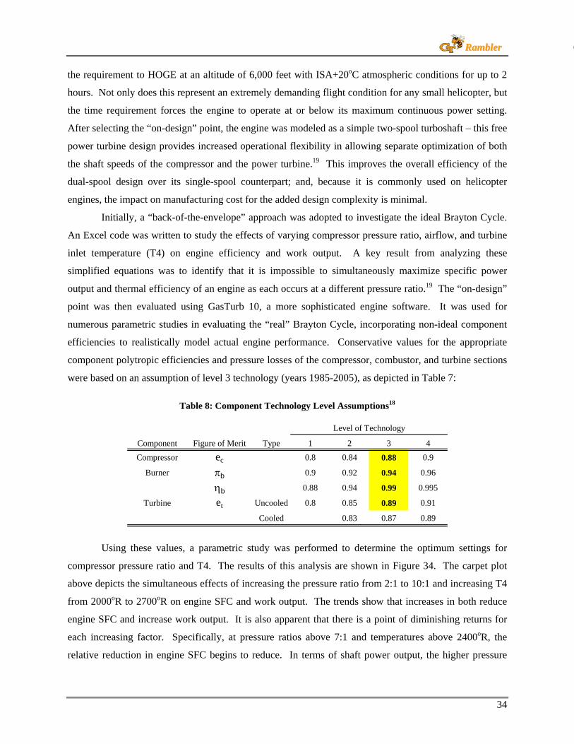
34

RRaammbblleerr

the requirement to HOGE at an altitude of 6,000 feet with ISA+20oC atmospheric conditions for up to 2

hours. Not only does this represent an extremely demanding flight condition for any small helicopter, but

the time requirement forces the engine to operate at or below its maximum continuous power setting.

After selecting the “on-design” point, the engine was modeled as a simple two-spool turboshaft – this free

power turbine design provides increased operational flexibility in allowing separate optimization of both

the shaft speeds of the compressor and the power turbine.19 This improves the overall efficiency of the

dual-spool design over its single-spool counterpart; and, because it is commonly used on helicopter

engines, the impact on manufacturing cost for the added design complexity is minimal.

Initially, a “back-of-the-envelope” approach was adopted to investigate the ideal Brayton Cycle.

An Excel code was written to study the effects of varying compressor pressure ratio, airflow, and turbine

inlet temperature (T4) on engine efficiency and work output. A key result from analyzing these

simplified equations was to identify that it is impossible to simultaneously maximize specific power

output and thermal efficiency of an engine as each occurs at a different pressure ratio.19 The “on-design”

point was then evaluated using GasTurb 10, a more sophisticated engine software. It was used for

numerous parametric studies in evaluating the “real” Brayton Cycle, incorporating non-ideal component

efficiencies to realistically model actual engine performance. Conservative values for the appropriate

component polytropic efficiencies and pressure losses of the compressor, combustor, and turbine sections

were based on an assumption of level 3 technology (years 1985-2005), as depicted in Table 7:

Table 8: Component Technology Level Assumptions18

Component Figure of Merit Type 1 2 3 4

Compressor ec 0.8 0.84 0.88 0.9

Burner πb 0.9 0.92 0.94 0.96

ηb 0.88 0.94 0.99 0.995

Turbine et Uncooled 0.8 0.85 0.89 0.91

Cooled 0.83 0.87 0.89

Level of Technology

Using these values, a parametric study was performed to determine the optimum settings for

compressor pressure ratio and T4. The results of this analysis are shown in Figure 34. The carpet plot

above depicts the simultaneous effects of increasing the pressure ratio from 2:1 to 10:1 and increasing T4

from 2000oR to 2700oR on engine SFC and work output. The trends show that increases in both reduce

engine SFC and increase work output. It is also apparent that there is a point of diminishing returns for

each increasing factor. Specifically, at pressure ratios above 7:1 and temperatures above 2400oR, the

relative reduction in engine SFC begins to reduce. In terms of shaft power output, the higher pressure

35

RRaammbblleerr

ratios considered provide minimal benefit, whereas, higher T4 clearly have an advantage in terms of

extracting more work from a given flow.

6.2.1 Turbine Cooling Trade Study

The benefits of increasing T4 do not come without penalty as at temperatures above 2300oR,

(1278oK) the turbine blades require cooling airflow to maintain material integrity. Figure 35

demonstrates the relationship between T4 and required turbine cooling as a function of the current level of

technology. A trade study was conducted to determine if the benefits of increasing T4 above 2300oR are

worth the increased design complexity required to cool the turbine blades. Since the power output

requirements for a small training helicopter are relatively less important than its overall operating

efficiency, SFC was used for evaluation. In order to calculate the percentage of bleed air required to

effectively cool the turbine blades at a given temperature, an Excel code was written to evaluate the

turbine cooling algorithm described in the NASA Technical Memorandum 81453.20 Figure 36 shows the

effect of increasing T4 from 2300oR to 2900oR on engine SFC. It was concluded that reduction in SFC,

less than 0.01 lb/HP/hr, did not outweigh the added manufacturing cost for providing cooling air to the

turbine blades. The added cost would be compounded by the small size of the turbine blades required for

this specific engine design.

2

8

3

765

4

1092000 2100 2200 24002300 270026002500

2

8

3

765

4

1092000 2100 2200 24002300 270026002500

Figure 34: “On-Design” Point Parametric Analysis

36

RRaammbblleerr

Turbine Cooling Trade Study

0.49

0.495

0.5

0.505

0.51

2200 2300 2400 2500 2600 2700 2800 2900 3000

Turbine Inlet Temperature (oR)

Specific Fuel

Consumption [lb/HP/hr]

Figure 35: Turbine Cooling Technology Assessment 21 Figure 36: Turbine Cooling Trade Study

6.2.2 Parametric Cycle Analysis Conclusions

Optimizing the engine “on-design” performance was an iterative process based on the

helicopter’s varying aerodynamic performance. The baseline vehicle design was continually being

updated and refined to reflect the analysis completed by each individual design discipline. Ultimately, a

power required value of 120 HP was determined as the necessary engine output. Given the maximum T4

as 2300oR and the component efficiencies described in Table 1, the optimization feature of GasTurb 10

was used to determine the optimum settings for airflow (1.04 lbm/s) and pressure ratio (6.5:1) that would

minimize the engine’s SFC with an output of 120 HP.

6.3 Performance Cycle Analysis

In order to achieve greater accuracy and detail than offered by the GasTurb 10 program for the

“off-design” performance, a model using the NASA Engine Performance Program (NEPP) was developed

NEPP, originally developed and used as the primary aircraft engine analysis tool at NASA-Lewis

Research Center, utilizes a FORTRAN code to calculate 1-dimensional, steady-state thermodynamic

performance for gas turbine engines.22 Figure 37 depicts the initial model used in NEPP.

A B D GC E HF I J

LOAD

Compressor Shaft

Power Turbine Shaft

1 765432 111098

A – InletB – DuctC – CompressorD – DuctE – CombustorF – High Pressure TurbineG – DuctH – Low Pressure TurbineI – DuctJ - Exhaust

Figure 37: NEPP Engine Model

37

RRaammbblleerr

As the figure demonstrates, the NEPP model consists of a series of components linked by station

properties that describe the flow properties at the entrance and exit of every component. The individual

properties of each physical component are included in the input code – this code also ensures that the

engine is properly arranged to model the desired flowpath. The NEPP input file includes non-physical

components which are used to “control, optimize, limit, and schedule engine variables.”22 The user can

define the appropriate engine flight conditions for the specific “off-design” points being evaluated.

Typically, these inputs consist of a series of changing altitude, airspeed, and throttle settings in order to

capture the engine’s performance characteristics throughout its entire operational, or flight, envelope.

The flight envelope for this training helicopter was an airspeed ranging from hover to Mach 0.2

(132 knots at SLS) and an altitude ranging from sea-level to 12,000 feet. 12,000 feet was selected as a

reasonable maximum altitude for a small training helicopter because the effects of reduced oxygen at

altitudes any higher can begin to impair a pilot’s responsiveness. FAA Regulations stipulate that all

aircraft crewmembers operating above 14,000 feet altitude, or above 12,500 feet altitude for a period of

more than 30 minutes, must have supplemental oxygen available. The NEPP model did not support the

evaluation of negative airspeeds to simulate rearward flight and therefore these flight conditions were not

considered part of the operational flight envelope. Although a rearward flight profile up to 20-30 knots is

possible in a small training helicopter, its influence on engine performance was assumed to be negligible.

6.3.1 Component Performance Maps

In addition to establishing the flight envelope, the “off-design” analysis in NEPP also required the

use of “maps” to better describe the thermodynamic performance of each individual component over its

actual range of operation.18 For the conceptual level of detail required on this project, a collection of

various tools and methods was used to produce a set of approximated component maps for the compressor

and turbine sections only. The details of these maps will be covered later in this report. For this analysis,

a constant level of combustion efficiency and pressure loss were considered adequate.

6.4 Component Design Considerations

6.4.1 Compressor Configuration Selection

An examination of preliminary compressor and turbine component design was undertaken with

the intent of providing a “feasibility” check for the parameters used throughout the engine cycle analysis.

Since the engine cycle analysis revealed that the optimum compressor pressure ratio for this application

was 6.5:1 at the “on-design” point, consideration had to be given to determining the optimum compressor

configuration that would achieve such results and maintain design simplicity. Although axial compressors

38

RRaammbblleerr

show better efficiency when compared to centrifugal compressors, at mass flow rates below 3 lbm/s, the

latter is more efficient due to its lower sensitivity to effects of blade tip clearance.16 In engines with

extremely low mass flow rates, axial compressors also exhibit another problem with manufacturability of

the last compressor stages as the blade tips can become too short.19 Therefore, a single-stage centrifugal

compressor configuration was selected in order to take advantage of the relative increased efficiency and

overall design simplicity. As per a discussion with Dr. David Eames of Rolls-Royce North America on

compressor design, the assumption that a single-stage radial compressor can achieve a 6.5:1 pressure ratio

was considered reasonable.

6.4.2 Centrifugal Compressor Design

In order to determine the geometric and performance characteristics of a centrifugal compressor,

an Excel code was written to mirror the sample problem calculations and techniques described in

Introduction to Turbomachinery.23 An iterative process of solving the entrance velocity triangle by

guessing the inlet Mach number at the tip, M1t, and then continuously calculating a new value for M1t until

the two converge, was used. The exit velocity triangle was calculated using the same iterative process for

the exit Mach number, M3t. The Wiesner correlation was also used to estimate the exit slip factor, σ,

defined as the ratio of exit swirl velocity to the rotor speed, as shown in Equation 3:

7.02b

Z)cos(

1β

−=σ Equation 3

where β2b= 0 for high speed impellers and Z is defined as the number of blades.23 By using the exit

dimensions and flow conditions of the axial compressor as the entrance conditions for the centrifugal

compressor, a preliminary design that would meet the necessary stage pressure ratio requirements was

determined. A conservative polytropic efficiency of 85% was assumed to account for the increased losses

associated with turbomachinery of this size. Figure 38 shows the component map used for the centrifugal

compressor, depicting efficiency and pressure ratio as a function of corrected flow and corrected speed.

Figure 38: Centrifugal Compressor Performance Map

Centrifugal Compressor Map (1 of 2)

0.74

0.75

0.76

0.77

0.78

0.79

0.8

0.81

0.82

0.4 0.6 0.8 1 1.2

Corrected Flow (lbm/s)

Efficiency

Speed = 0.6 Speed = 0.7 Speed = 0.8


Centrifugal Compressor Map (2 of 2)

012345678

0.4 0.6 0.8 1 1.2

Corrected Flow (lbm/s)

PressureRatio



39

RRaammbblleerr

6.4.3 Turbine Section Design

Using Turbine Preliminary Design Program (TURBN), a program within Mattingly’s Aircraft

Engine Design textbook software suite, initial sizing and performance characteristics for both the high

pressure and power turbines were completed. The engine output data from NEPP provided the required

input. The following assumptions were made: two-dimensional flow, constant axial velocity, constant

mean radius, adiabatic flow in the rotor and stator and calorically perfect gas.18 The assumption of 89%

polytropic efficiency was made for both turbines based on the reference in Table 1 of this report. Table 8

summarizes the results for this single stage high pressure and single stage low pressure turbine design.

The material selection for the both turbine disks was based on an analysis of the blade stress factor, AN2,

and their shaft speeds. For the high pressure turbine, a shaft speed of 60,000 RPM was selected in order

to achieve a design balance between the competing demands of compressor performance and maximum

turbine blade stress. At speeds higher than 60,000 RPM the high pressure turbine blade stress increases to

a level that exceeds its uncooled material limitations.

Table 9: Turbine Design Parameters

HPT LPT UnitsStage Efficiency ηs 0.900 0.882

Stage Pressure Ratio πs 2.40 1.29Inlet Temperature T4 2300 1922 oR

Hub Radius rh 1.86 3.60 inTip Radius rt 2.14 3.90 in

Hub-to-Tip Ratio rh/rt 0.87 0.92

Reaction oRc 0.54 0.55Loading Coefficient ψ 2.57 2.79

Flow Coefficient φ 1.01 1.07

Blade Stress Factor AN2 8.00E+09 4.34E+09 in2 RPM2

Material DS Superalloy Nickel Alloy

For the low pressure turbine, a shaft speed of 30,000 RPM was selected as the optimum value for

balancing the demands of material selection and turbine performance. This slower speed allows the use

of less expensive materials while maintaining a high level of stage efficiency. Figure 39 demonstrates the

relationship between the blade stress factor, AN2, and material specific strength for the high pressure and

low pressure turbines at an assumed taper ratio of 1.0. The graph indicates that the required specific

strength is approximately 700 psi/(slugs/ft3) for the high pressure turbine and 400 psi/(slugs/ft3) for the

low pressure turbine. These values were used on the graph in Figure 40 to determine the turbine materials

required to meet the high temperature demands. This plot shows that the high pressure turbine should be

constructed from “Material 5” which refers to a single-crystal or directionally solidified (DS) superalloy

40

RRaammbblleerr

and the low pressure, or power, turbine should be constructed from “Material 3” which refers to a

wrought nickel alloy.

HPTLPT HPTLPT

HPT

LPT

HPT

LPT

Figure 39: Blade Stress vs. Specific Strength18 Figure 40: Turbine Material Selection Plot 18

For the turbine performance map, the parameters typically used are total pressure ratio, corrected

mass flow rate, corrected engine speed, and adiabatic efficiency. A combination of tools was used to

generate both the high pressure turbine (HPT) and power turbine (PT) maps for this project. GasTurb 10

was used to produce the scaled turbine maps; however, instead of manually converting this graphical

output into the format needed for NEPP, a NASA program known as the Extended Parametric

Representation of Turbines (PART) was used to produce the maps in the proper NEPP format using the

input data from GasTurb 10.24 Figures 41 and 42 show turbine performance maps for the HPT and PT.

Figure 41: High Pressure Turbine Performance Map Figure 42: Power Turbine Performance Map

41

RRaammbblleerr

Using these inputs into NEPP, the performance cycle analysis was conducted iteratively with the

vehicle sizing and performance code. Both the Rf Excel program and GTPDP incorporated an engine

model to more accurately predict the fuel and power requirements at changing altitudes. This model was

refined and updated to reflect the changing engine performance characteristics until a final solution was

achieved that most effectively satisfied the performance requirements with the lowest SFC.

6.4.4 Combustion Section Design

A reverse-flow cannular combustor design was selected for this engine configuration. This

design provided the most efficient optimization of space within the engine’s core. The increased frontal

area required for the centrifugal compressor stage allowed the reverse-flow cannular combustor to be

located outside of the high pressure turbine’s radius. For a preliminary sizing estimate, the dimensions of

an existing combustor design were linearly reduced in order to determine the appropriate scale for this

engine application.25 The technology level assumptions of a combustor efficiency of 99% and a

combustion pressure drop of 6%, described in Table 1 of this report, were used within the NEPP model.

6.4.5 Modular Gearbox Design

A modular approach was used in the design of the engine gearbox in order to capitalize on

increased marketability. Two separate gearbox configurations, turboshaft and turboprop, are designed to

provide greater flexibility in using the engine for both rotary-wing and fixed-wing applications. The

turboshaft engine gearbox provides a 5:1 reduction ratio for the main drive shaft and a 5.8:1 reduction

ratio for the tail rotor drive shaft. This gearbox configuration extends below the engine core to provide

clearance for the tail rotor drive shaft (See Diagram Sheets 2 and 4). The turboprop gearbox does not

include the gear reduction for tail rotor driveshaft and, therefore, maintains a smaller cross-sectional size

better suited for fixed-wing applications.

The material selected for the gears is case hardened steel or VASCO X2M. It exhibits high

strength, high hardness, high temperature capability, while maintaining light weight properties relative to

other steels.26 An additional gear reduction ratio of 4:1 was included in the engine gearbox for the starter

configuration and was connected to the compressor shaft. Through the use of a starter-generator and

battery power, the compressor can be operated during the engine starting sequence to initially provide the

necessary air compression for successful combustion.

In order to meet autorotational requirements inherent to any helicopter gear train design, a

freewheeling unit with a sprag clutch was also incorporated into the connection between the power

turbine shaft and the engine gearbox. This component “provides the means to disconnect the power train

from a failed or secured engine.”27 The engine drives an outer gear ring which engages an inner gear ring

42

RRaammbblleerr

connected to the rest of the engine gearbox during normal powered operation. In the event of an engine

failure, the outer gear ring will stop, allowing the inner gear ring to continue rotating. This mechanical

design allows both the main rotor and tail rotor to continue in autorotation following an engine failure.

6.5 Specifications and Performance Analysis

Using the maximum continuous power (MCP) setting for sea-level standard conditions of 152 HP

calculated using NEPP, it was necessary to establish an estimated value for the 5-minute maximum

takeoff power requirement as stipulated in Federal Aviation Regulation (FAR) Part 27. Equation 4 was

used to estimate this short duration power:

)e252.01(HPHP t0173.0NRSD

−+= Equation 4 where HPNR refers to normal rated power (replaced by MCP) and t is the time in minutes.7 Based on

these results, the NEPP model was updated to reflect the increased throttle settings required to generate

the increased power demand by allowing the turbine inlet temperature to increase from 2300oR at the

MCP setting to 2450oR for the 5- minute takeoff power setting. Figures 43-48 depict the overall engine

performance throughout its full operational envelope and at varying atmospheric conditions:

Engine Performance (ISA Conditions)

0

50

100

150

200

0 2000 4000 6000 8000 10000 12000

Altitude (ft)

HPAv ail

TO Pow er (5 min)

Max Continuous Pow er

Engine Performance (ISA+20oC Conditions)

0

50

100

150

200

0 2000 4000 6000 8000 10000 12000

Altitude (ft)

HPAv ail

TO Power (5 min)

M ax Continuous Power

Figure 43: HP Available vs. Altitude (ISA) Figure 44: HP Available vs. Altitude (ISA+20oC)

Engine Performance (TO Power)

0

20

40

60

80

100

120

0 2000 4000 6000 8000 10000 12000

Altitude (ft)

FF[lb/hr]l

ISA+20CISAISA-20C

Engine Performance (Max Continuous Power)

0

20

40

60

80

100

120

0 2000 4000 6000 8000 10000 12000

Altitude (ft)

FF[lb/hr]l

ISA+20CISAISA-20C

Figure 45: Fuel Flow vs. Altitude (TOP) Figure 46: Fuel Flow vs. Altitude (MCP)

43

RRaammbblleerr

Engine Performance (TO Power)

0.45

0.46

0.47

0.48

0.49

0.50

0.51

0.52

0 2000 4000 6000 8000 10000 12000

Altitude (ft)

SFC[lb/HP/hr]l

ISA+20CISAISA-20C

Engine Performance (Max Continuous Power)

0.45

0.46

0.47

0.48

0.49

0.50

0.51

0.52

0 2000 4000 6000 8000 10000 12000

Altitude (ft)

SFC[lb/HP/hr]l

ISA+20CISAISA-20C

Figure 47: SFC vs. Altitude (TOP) Figure 48: SFC vs. Altitude (MCP)

6.6 Weight Analysis

CATIA was used to determine the specific volume of each major engine component. These

values were then evaluated as a function of their material density to determine an estimated weight

breakdown. Table 9 summarizes the results of this analysis.

Table 10: Engine Component Weight Breakdown

Component Volume (in3) Density (lb/in3) Weight (lb)Compressor 35.20 0.170 6.0Combustor 18.60 0.283 5.3

High Pressure Turbine 12.97 0.298 3.9Low Pressure Turbine 24.06 0.298 7.2

Compressor Shaft 11.88 0.298 3.5Power Turbine Shaft 7.58 0.276 2.1

Gearbox 220.96 0.283 / 0.098 51.9Housing 141.99 0.283 40.2

Total Weight 120.0

6.7 Manufacturing

The small sizes of the engine’s rotating components require the use of state-of-the-art

manufacturing technologies in order to achieve the close material tolerances needed for high efficiency.

For the centrifugal compressor, a Computer Numerically Controlled (CNC) five-axis milling machine

will be used to precisely machine its complex geometry. The tool path programs which define the

intricacies of the cutting motions are easily generated using a suite of CAD/CAM software. As future

improvements are made in the aerodynamic design of the radial compressor using computational fluid

dynamics (CFD) analysis, the five-axis milling machine can immediately update its tool paths to capture

44

RRaammbblleerr

the design upgrades without an engineering compromise for manufacturability. This integration between

the design and manufacturing steps increases both process efficiency and component efficiency.

The turbine section of the engine will utilize directional solidification to produce the high

pressure turbine blades with a vacuum chamber casting process. By closely controlling the temperature

of the casting process, directional solidification results in a turbine airfoil composed of columnar grains

along its spanwise axis. This grain alignment strengthens the blade and effectively eliminates the

potential for destructive intergranular crack initiation.28 Although more expensive to manufacture, the

structural benefits offset this cost by reducing the long term maintenance requirements of the engine’s

turbine section. Directionally solidified superalloys exhibit increased ductility and fatigue life which will

lengthen the time between overhaul (TBO) for the entire engine. For the low pressure turbine, which

experiences lower relative temperatures, an integrally cast turbine wheel and blades will be used in order

to reduce part count, manufacturing time, and overall complexity.

6.8 Federal Aviation Regulations (FAR) Requirements

A new engine design is subject to the Code of Federal Regulations, Title 14 – Aeronautics and

Space, Chapter 1 – Federal Aviation Administration, Subchapter C – Aircraft, Part 27 – Airworthiness

Standards: Normal Category Rotorcraft and Part 33 – Airworthiness Standards: Aircraft Engines.

Beginning with Part 27, this regulation lists numerous requirements in Subpart E – Powerplant, Table 10

highlights those that are applicable at this conceptual level of engine design:

Table 11: FAR Part 27 Engine Requirements Para. Title Summary 27.907 Engine Vibration Engine and rotor drive system must be free from excessive vibrations

-- Transmission mounted with dampers to eliminate excessive vibrations due to the rotor 27.917 Rotor Drive System Design Engine must automatically disengage from rotor drive system for autorotational capability

-- Freewheeling unit installed in engine gearbox

27.1091 Air InductionInlets must supply the engine with the required air during all operating conditions and minimize the ingestion of debris-- Screened engine cowling and inlet barrier filters surround the engine inlet

27.1093 Induction System Icing PreventionEngine must be capable of operating at all power settings without accumulating ice on the inlet detrimental to engine operation-- Engine anti-ice system uses bleed air from the compressor to heat the walls of the engine

27.1141 Powerplant Controls: GeneralNo single point failure in any powerplant control system can cause the loss of a powerplant function necessary for safety-- FADEC engine control has an analog backup mode

27.1191 FirewallsEngine must be isolated from personnel compartments, structures, controls, and rotor mechanisms by a firewall or shroud-- Engine compartment is isolated

For Part 33, this regulation is more focused on the specific testing and evaluation requirements

used during the certification process of a new aircraft engine. Table 11 summarizes the applicable

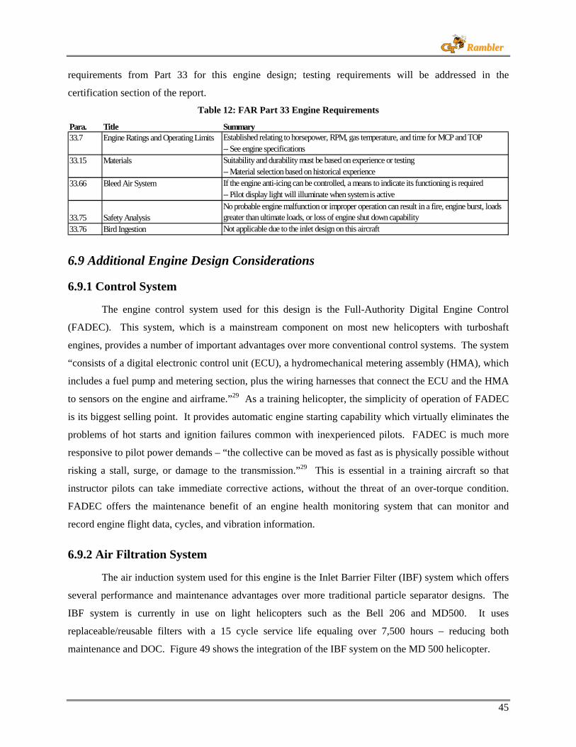
45

RRaammbblleerr

requirements from Part 33 for this engine design; testing requirements will be addressed in the

certification section of the report.

Table 12: FAR Part 33 Engine Requirements

Para. Title Summary 33.7 Engine Ratings and Operating Limits Established relating to horsepower, RPM, gas temperature, and time for MCP and TOP

-- See engine specifications33.15 Materials Suitability and durability must be based on experience or testing

-- Material selection based on historical experience33.66 Bleed Air System If the engine anti-icing can be controlled, a means to indicate its functioning is required

-- Pilot display light will illuminate when system is active

33.75 Safety AnalysisNo probable engine malfunction or improper operation can result in a fire, engine burst, loads greater than ultimate loads, or loss of engine shut down capability

33.76 Bird Ingestion Not applicable due to the inlet design on this aircraft

6.9 Additional Engine Design Considerations

6.9.1 Control System

The engine control system used for this design is the Full-Authority Digital Engine Control

(FADEC). This system, which is a mainstream component on most new helicopters with turboshaft

engines, provides a number of important advantages over more conventional control systems. The system

“consists of a digital electronic control unit (ECU), a hydromechanical metering assembly (HMA), which

includes a fuel pump and metering section, plus the wiring harnesses that connect the ECU and the HMA

to sensors on the engine and airframe.”29 As a training helicopter, the simplicity of operation of FADEC

is its biggest selling point. It provides automatic engine starting capability which virtually eliminates the

problems of hot starts and ignition failures common with inexperienced pilots. FADEC is much more

responsive to pilot power demands – “the collective can be moved as fast as is physically possible without

risking a stall, surge, or damage to the transmission.”29 This is essential in a training aircraft so that

instructor pilots can take immediate corrective actions, without the threat of an over-torque condition.

FADEC offers the maintenance benefit of an engine health monitoring system that can monitor and

record engine flight data, cycles, and vibration information.

6.9.2 Air Filtration System

The air induction system used for this engine is the Inlet Barrier Filter (IBF) system which offers

several performance and maintenance advantages over more traditional particle separator designs. The

IBF system is currently in use on light helicopters such as the Bell 206 and MD500. It uses

replaceable/reusable filters with a 15 cycle service life equaling over 7,500 hours – reducing both

maintenance and DOC. Figure 49 shows the integration of the IBF system on the MD 500 helicopter.

46

RRaammbblleerr

Figure 49: Inlet Barrier Filter (IBF) System on the MD 500 30

The IBF system filters over 99% of the particles in the airflow in order to create a cleaner plenum

chamber for the engine inlet – improving engine component protection from foreign object damage

(FOD) and overall engine performance by increasing the temperature margin.30 The only drawback of

this system is that it requires the installation of a bypass door to allow unfiltered air to enter the engine in

the event that a filter becomes completely blocked. However, the system is designed to provide the pilot

with a cockpit indication of an impending bypass condition – allowing several flight hours to take

corrective action before a full bypass would be required.

6.10 Transmission Design

See Diagram Sheet 4 for a complete drive train schematic.

6.10.1 Configuration Selection

Based on the relatively low horsepower output of the Rambler’s new engine, it was determined

that a new transmission design would also be required in order to maintain design simplicity and to

incorporate potential weight saving measures. For this transmission, a simplified split torque

transmission design was selected which demonstrates several key advantages over a more conventional

planetary gearbox design. The general configuration of this transmission followed the design presented

by Mr. Thomas Hanson in his report, A Designer Friendly Handbook of Helicopter Rotor Hubs. The

Hanson transmission provided an optimized integration of the hub configuration selected for this vehicle

and its propulsion source by minimizing the design complexity and increasing the structural integrity of

the overall drive system. The Hanson transmission design utilized a combination of only four main gears

to achieve the required gear reduction between the engine and the rotor system and this reduction in parts

directly translated to savings in both overall weight and cost. This design also offered a much lower

dimensional profile than that of a conventional planetary system which minimized its drag profile and

allowed much greater design flexibility in integrating the transmission with the airframe structure. Figure

47

RRaammbblleerr

50 depicts this simplified gearbox configuration and Figure 51 shows a Hanson transmission built as part

of his light helicopter and auto-giro prototype projects.

BullGear

Follow Gear Drive Gear

LeadGear

Figure 50: Hanson Transmission Gears Figure 51: Actual Hanson Transmission

The Hanson transmission clearly offered the most robust solution in terms of structural

redundancy by using the combination of a rotating and non-rotating mast to transmit loads between the

rotor and the fuselage. The short length and large diameter of the rotating mast, which is attached directly

to the bull gear, provides “the lightest way to carry the rotor drive torque to the hub.”1 The non-rotating

mast is located inside of the rotating mast with a connection at the base of the transmission housing. This

second mast provides structural redundancy in the case of a main rotor shaft failure and protection for the

aircraft’s flight controls which are located inside, thus increasing the overall safety of this design.

6.10.2 Sizing and Analysis

The Hanson transmission’s individual gears were assumed to be a standard spur gear

configuration instead of a helical gear design. Although the helical gear design offers advantages in noise

reduction and improved load sharing capacity, the spur gear configuration simplifies the overall design by

eliminating the need for thrust bearings because spur gears do not generate axial loads or thrust.26

Ultimately, this translates to a lighter gearbox with lower manufacturing cost. The reduced capability of

spur gears is not a limiting factor because this transmission’s load requirements are relatively small. The

following list of initial design conditions and assumptions was used to analyze the individual gear sizing

and performance characteristics:

Maximum transmission power rating > 200 HP

Main rotor rotational speed = 509 RPM

Engine gearbox output speed = 6,000 RPM

Transmission gearbox TBO = 3,500 hours

Using these initial conditions, each gear mesh was evaluated to determine the optimum pitch diameter and

number of teeth. Table 12 shows the results of this study.

48

RRaammbblleerr

Table 13: Transmission Gear Sizing

Drive Gear Lead Gear Follow Gear Bull Gear UnitsPitch Diameter 2 3.5 4 12 in

Teeth 16 28 32 96Face Width 2.5 2.5 2.5 1 in

Material -------------- VASCO X2M Steel --------------

VASCO X2M Steel was selected as the material for these gears for the same reasons listed in the engine

gearbox section – its high strength, hardness, and temperature capability relative to other steels. Based on

these gear geometries, the contact stress and bending stress calculations were performed using the

techniques and procedures presented in CPT Andrew Bellocchio Masters Thesis report.26 Equations 5

and 6 were used to calculate the contact stress and bending stress for each gear.

IC

dFK

KKKWCs fmsvotpc =

Equation 5: Actual Contact Stress

Where: sc = contact stress (lb/in2) Cp = elastic coefficient (lb/in2)0.5 Wt = transmitted tangential load (lb) Ko = overload factor Kv = dynamic factor Ks = size factor Km = load distribution factor Cf = surface condition factor (pitting resistance) F = net face width (in) I = geometry factor for pitting resistance d = operating pitch diameter of pinion (in)

JKK

FP

KKKWs Bmdsvott =

Equation 6: Actual Bending Stress

Where: st = bending stress (lb/in2) KB = rim thickness factor J = geometry factor for bending strength Pd = transverse diametral pitch (in-1)

Results were compared to the maximum working stress values using Equations 7 and 8, where “working”

stress refers to the allowable stress corrected for stress cycles, reliability, and temperature effects.

R

H

T

N

H

acc K

CKZ

Ss

s ≤

Equation 7: Working Contact Stress Where: sac = allowable contact stress (lb/in2) ZN = stress cycle factor CH = hardness ratio factor SH = safety factor KT = temperature factor KR = reliability factor

RTF

Natt KKS

Yss ≤

Equation 8: Working Bending Stress

Where: sat = allowable bending stress (lb/in2) YN = stress cycle factor SF = safety factor KT = temperature factor KR = reliability factor

49

RRaammbblleerr

Based on the assumption of a 3,500 hour gear life, the stress cycles experienced by each gear

mesh were on the order of magnitude of 108 total cycles. Therefore, the stress cycle factors, ZN and YN,

were used to more accurately estimate the effects of fatigue in the life of each gear. The TO power

transmission limit was then established by iterating these equations until a limiting power relationship

developed in which the actual stress equaled the maximum allowable working stress. As illustrated in

Table 13, the lead-bull gear mesh was the limiting configuration with a maximum TO power rating of 203

HP. The maximum continuous transmission power was calculated to be 168 HP based on the assumption

of a 10% buffer between the actual stress and the maximum allowable working stress.

Table 14: Transmission Gear Stress (TO Power Rating)

Units

Diametrical Pitch teeth / inGear Ratio

RPM RPM

Drive Lead Drive Follow Lead Bull Follow BullContact Stress 176,726 173,171 174,100 170,007 181,499 174,414 169,857 163,794 psi

Allowable Contact Stress 177,645 181,509 177,645 182,445 181,499 190,360 182,422 190,346 psi

Bending Stress 21,910 18,552 21,761 17,692 17,957 36,238 16,937 36,022 psiAllowable Bending Stress 39,490 40,041 39,490 40,174 40,040 41,284 40,171 41,282 psi

Drive-Lead8

1.75

Drive-Follow82

Follow-Bull83

1523 / 509

8Lead-Bull

3.431743 / 5093046 / 1743 3046 / 1523

6.10.3 Auxiliary Gearbox

There is a 90o direction change required between the engine’s main output shaft and the

transmission’s drive gear; therefore, an auxiliary gearbox was installed which houses a single bevel gear

connection. This gearbox has the following characteristics described in the Table 14.

Table 15: Auxiliary Gearbox Stress (TO Power)

Engine Output Transmission Input Units

Diametrical Pitch teeth / inBevel Gear Ratio

RPM 6000 3046 RPMPitch Diameter 3.22 6.33 in

Contact Stress 152,410 152,410 psiAllowable Contact Stress 225,445 234,805 psi

Bending Stress 21,679 25,109 psiAllowable Bending Stress 38,832 27,641 psi

91.97

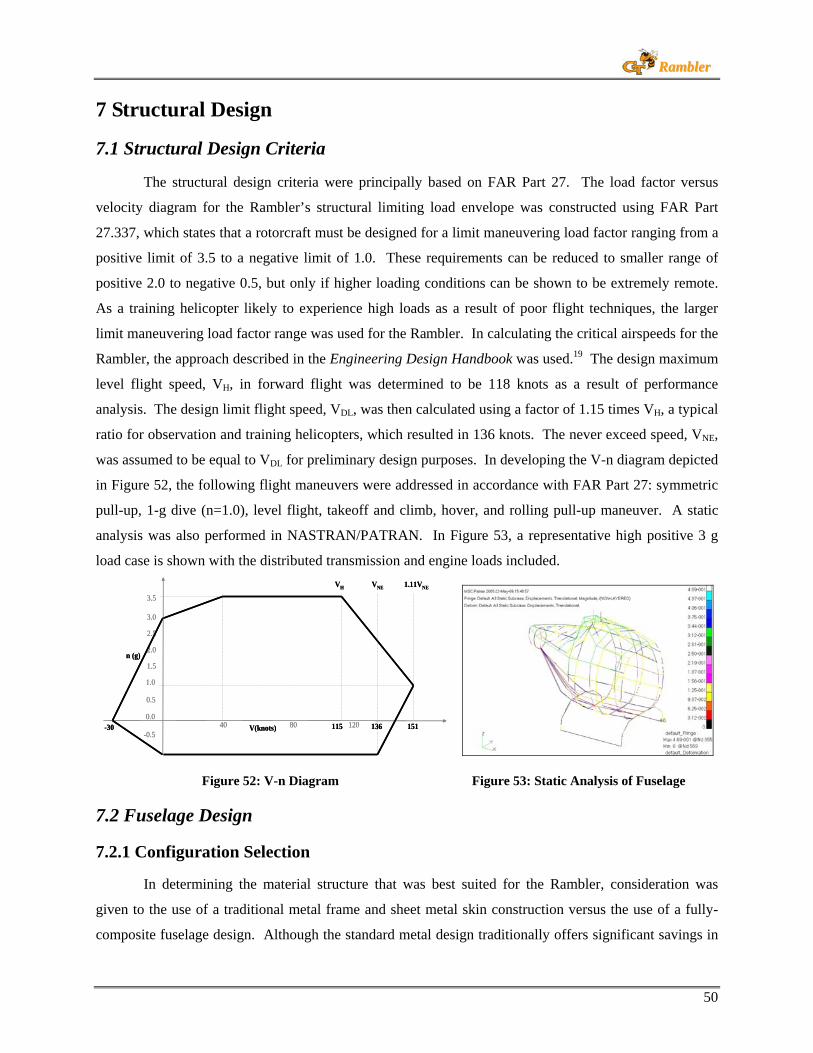
50

RRaammbblleerr

7 Structural Design

7.1 Structural Design Criteria

The structural design criteria were principally based on FAR Part 27. The load factor versus

velocity diagram for the Rambler’s structural limiting load envelope was constructed using FAR Part

27.337, which states that a rotorcraft must be designed for a limit maneuvering load factor ranging from a

positive limit of 3.5 to a negative limit of 1.0. These requirements can be reduced to smaller range of

positive 2.0 to negative 0.5, but only if higher loading conditions can be shown to be extremely remote.

As a training helicopter likely to experience high loads as a result of poor flight techniques, the larger

limit maneuvering load factor range was used for the Rambler. In calculating the critical airspeeds for the

Rambler, the approach described in the Engineering Design Handbook was used.19 The design maximum

level flight speed, VH, in forward flight was determined to be 118 knots as a result of performance

analysis. The design limit flight speed, VDL, was then calculated using a factor of 1.15 times VH, a typical

ratio for observation and training helicopters, which resulted in 136 knots. The never exceed speed, VNE,

was assumed to be equal to VDL for preliminary design purposes. In developing the V-n diagram depicted

in Figure 52, the following flight maneuvers were addressed in accordance with FAR Part 27: symmetric

pull-up, 1-g dive (n=1.0), level flight, takeoff and climb, hover, and rolling pull-up maneuver. A static

analysis was also performed in NASTRAN/PATRAN. In Figure 53, a representative high positive 3 g

load case is shown with the distributed transmission and engine loads included.

n (g)

V(knots)

3.5

2.5

-0.5

0.0

1.5

2.0

VNEVH

40 136

1.11VNE

15180 120115

1.0

3.0

0.5

-30

n (g)

V(knots)

3.5

2.5

-0.5

0.0

1.5

2.0

VNEVH

40 136

1.11VNE

15180 120115

1.0

3.0

0.5

-30

Figure 52: V-n Diagram Figure 53: Static Analysis of Fuselage

7.2 Fuselage Design


In determining the material structure that was best suited for the Rambler, consideration was

given to the use of a traditional metal frame and sheet metal skin construction versus the use of a fully-

composite fuselage design. Although the standard metal design traditionally offers significant savings in

51

RRaammbblleerr

production cost over composite construction, emerging technologies are quickly bridging this financial

gap. Using the Bell Cost Model31, a material selection trade study indicated that a composite fuselage

would only cost 7.8% more than metal – accounting for an overall increase of less than 1% of the

vehicle’s total production cost. Despite this minor disadvantage, composite materials offer critical weight

savings over metal construction and they are superior to metals in resistance to corrosion, reducing the

overall maintenance requirements and direct operating cost. In a research effort conducted by NASA and

the US Army Research Laboratory in 1999, a 1/5 scale composite fuselage – designed for light aircraft

and rotorcraft applications – was shown both experimentally and analytically to achieve improved

crashworthiness results.32 The goal of this research program was “to demonstrate a new fuselage concept

for improved crashworthiness, which can be fabricated using low-cost materials and manufacturing

techniques.”32 A similar composite design was selected for the Rambler to capitalize on cost and weight

savings, improved reliability, and increased safety.

7.2.2 Composite Structure

The details of the Rambler’s composite fuselage design were largely based on the findings

presented in the previously mentioned NASA Report. The characteristics and materials selected for this

design are depicted in Figure 54. The exterior contour and dimensions were driven by human size factors

and consideration of the ergonomics required to safely adjust the flight controls. From the crashworthy

design perspective, the fuselage’s upper section was designed to be stiff, yet frangible enough to deform

during a crash sequence, thus protecting the occupants by dissipating the energy in doing deformation

work. Hence, a relatively low stiffness E glass/epoxy skin was chosen for the fuselage with a foam core

sandwiched between the inner and outer walls to further absorb the energy. The floor section materials

were selected in order to maintain high structural rigidity and minimize deformation upon impact;

therefore, a hybrid laminate of graphite/epoxy and E glass/epoxy that exhibits high stiffness and excellent

strength properties was used.

Graphite/Epoxy[0/90]ns

E-glass/Epoxy[0/90/45/-45]ns

Shock Absorbing

Foam

E-glass/Epoxy[0/90/]ns

Graphite/Epoxy[45/-45]ns

Energy Absorbing Sub-Floor

Hybrid Laminate[0G/90G/0/90/45/-45]ns

Graphite/Epoxy[0/90]ns

E-glass/Epoxy[0/90/45/-45]ns

Shock Absorbing

Foam

E-glass/Epoxy[0/90/]ns

Graphite/Epoxy[45/-45]ns

Energy Absorbing Sub-Floor

Hybrid Laminate[0G/90G/0/90/45/-45]ns

Figure 54: Composite Fuselage Design

52

RRaammbblleerr

The lower half of the fuselage was also designed to deform during a crash sequence and thus an E

glass/epoxy was used for this area. Finally, a foam-filled, energy absorbing sub-floor was implemented to

provide an additional source of energy dissipation. A structural redundancy in the form of a shear pin

between the L section floor beams was provided. During a crash, the shear pin will fail and cause the

disconnection of the lower L beam from the upper L beam, thus the energy would not be transferred to the

floor where the pilot seats are mounted. Figure 55 shows a detailed view of this safety feature.

In order to effectively compensate for the vertical load paths required for any vertical takeoff and

landing (VTOL) application, the Rambler’s structural design also incorporates a series of composite

stringers and ribs needed to take bending and shear loads. Specifically, this skeletal framework, directly

attached and co-cured with the inner walls of the fuselage, incorporates load paths within the fuselage

structure. In order to integrate their connection to the skid landing gear, a combination of two keel beams

running through the sub-floor along the longitudinal axis of the aircraft was used. Figure 56 shows the

primary structural load paths.

Shear Pin

L ShapedBracket

Aircraft Floor

Shear Pin

L ShapedBracket

Aircraft Floor

Figure 55: Keel Beam Detail Figure 56: Primary Structural Load Paths

7.2.3 Manufacturing

The Rambler’s fuselage manufacturing is based on the composite bonding of two halves similar

to that used by the Adam Aircraft Corporation.33 While the Adam Aircraft manufacturing methodology

of eliminating all stringers, longerons, spars, and ribs by laying the fiber at the orientation at which the

load path occurs is highly desired, such a composite fuselage without metal fittings has not been yet

demonstrated for rotorcraft technology. Hence, the Rambler design incorporates a more conservative

combination of metal fittings and composite cured and co-cured parts. An example is the Rambler’s use

of metal L shaped brackets along the inner wall of its composite fuselage over which the composite floor

beam will be bolted (Figure 55). Programmable Powder Preform Process (P4), a new and cost-effective

mold manufacturing technique, uses robotic choppers to spray short fibers onto glass to create the preform

for the structure. This process is followed by the injection of resin and curing in a mold, thus creating the

two fuselage outer and inner walls between which the foam will be glued. The upper and lower portions

of the fuselage will be manufactured using this technique and then connected to the floor.

53

RRaammbblleerr

7.3 Landing Gear


As a training helicopter that will likely experience numerous hard landings, the design of the

Rambler’s landing gear was considered in detail to ensure the crashworthiness of its configuration. A

standard skid landing gear configuration was selected for its overall design simplicity and robustness over

more expensive and complicated wheeled systems that employ shock absorbing oleo struts, etc. Although

these wheeled landing gears offer improved pilot and passenger comfort, in a training environment, the

“unforgiving” characteristics of skid landing gears are beneficial in developing a pilot’s control touch.

Ultimately, the skid landing gear design is lightweight, less expensive, easy to maintain, and capable of

withstanding high static and dynamic loads.

7.3.2 Dimensions and Materials

Based on a paper written by Tho, C. et al,34 the skid landing gear was designed using hollow

circular skid tubes and hollow box-section cross beams. The cross sectional dimensions of the circular

section had an outer diameter of 3 inches and an inner diameter of 2 inches; the rectangular cross section

had a width of 2 inches and a height of 1.5 inches. A representative thickness of 0.5 inches was selected

for both the circular skid tubes and the box-section cross beams. As depicted in Diagram Sheet 1, the

length of the skid tubes, width of the cross beams, and height of the landing gear above the ground were

finalized based on engineering judgment and fuselage design considerations.

Tungsten carbide was initially considered as the material for the landing gear in accordance with

the paper previously mentioned; however, despite its high strength characteristics, it is a very expensive

and dense material. Therefore, structural steel was selected as an alternative. With an ultimate tensile

strength (UTS) of 94 ksi and yield strength of 45 ksi, structural steel demonstrated the necessary

characteristics essential for a crashworthy design as shown in the next section of this report.

7.3.3 Crashworthiness Analysis

In accordance with the FAR Part 27.725 Limit Drop Test for rotorcraft landing gears, a

comprehensive analysis was performed in order to verify the crashworthiness of this landing gear design.

Additionally, FAR 27.501 stipulates certain testing requirements that are specific to skid landing gear

configurations, such as, the standard drop height of 13 inches must be increased by a factor of 1.5 with an

initial velocity of 109.77 in/sec. For this proposal, however, even more stringent US Navy standards

were used – a drop height of 25 inches and velocity of 122 in/sec – to ensure that federal crashworthiness

standards were exceeded. A finite element model was developed using ABAQUS. Initially, the landing

54

RRaammbblleerr

gear configuration was modeled using solid tetrahedral elements and the ground as an analytical rigid

surface (Figure 57). With a partitioned mesh, the model consisted of over 90,000 tetrahedral elements

requiring 5-6 days of computational run-time. Using the paper by Tho et al,34 a beam element model was

created to expedite the computational process.

The beam element model utilized a three-dimensional wireframe for the skid tubes and the cross

beams in which beam section circular pipe and rectangular box section profiles were assigned. The

following material properties of isotropic steel were then applied to the model: stiffness of 30 x 106 psi,

density of 0.283 lb/in3, and a plasticity stress-strain curve with yielding at 45 ksi and 1% plastic strain at

75 ksi. Beam section orientations were assigned, instances of the individual parts were created, and a

mesh independent assembly instance was created using B32 beam elements in ABAQUS. The fuselage

was represented as a rigid node with assigned mass and inertia properties and rigid beam connectors were

used to connect the fuselage node to the cross beams. The ground was meshed using four node shell

elements (S4R). Figure 58 shows the entire beam element model for the landing gear.

Using the beam element landing gear model, the total analysis time was reduced to 2-3 hours.

The total time step varied from 155-200 milliseconds depending upon the landing condition being

evaluated. In specifying the interaction properties between the landing gear and the ground, the following

assumptions were used: a static coefficient of friction of 0.5, a dynamic coefficient of friction of 0.35, a

decay coefficient of 0.05, and no ground separation after contact. A surface-to-surface master-slave

contact interaction was specified in which the ground was specified as the master surface and the bottom

of the skid tubes as the slave node region. In establishing the loads and boundary conditions, the ground

was rigidly fixed by activating the Encastre boundary condition, thus constraining all six degrees of

freedom, 1-g gravity load was activated over the entire landing gear model, and velocities along the

appropriate directions were prescribed according to the landing scenario being simulated. In accordance

Figure 58: Beam Element Model of Skid Landing Gear

Figure 57: Solid Model of Skid Landing Gear

55

RRaammbblleerr

with FAR requirements, four landing scenarios were modeled as follows: level landing on two skids,

pitch-down nose first landing, pitch-up aft first landing, and single skid rolling landing. Figures 59 and

60 show an example of the program output for the level landing and single skid landing conditions. Table

15 summarizes the results from all four landing modes analyzed using the bean element model.

Figure 59: Level Landing Figure 60: Landing on One Skid

Table 16: Limit Drop Test Results

Landing Condition

Max ObservedStress [ksi]

Max Allowable Stress for Rupture [ksi]

Level 75 94

Nose First 76 94

Aft First 78 94

Single Skid Rolling 81 94

The landing gear design of the Rambler exceeds the Federal requirements with the single skid rolling

landing condition exhibiting the highest observed stress of 81 ksi – 13 ksi below the material rupture limit

of isotropic steel. In each scenario, the landing gear experienced yielding without rupture, a key

characteristic of crashworthy landing gear design. This margin of error is important for training

helicopters where the probability of the aircraft sustaining a hard landing is dramatically increased.

7.3.4 Landing Gear Dampers

Based on the ground resonance phenomenon and the available lead-lag damping inherent in the

Hanson rotor system, lead-lag dampers may not be required. However, dampers can be provided on the

cross beam of the skid, if necessary. The Deutsch criterion would be used to determine the damping

required by considering the product of the blade lag damping and the fixed system damping effective at

the hub.35

56

RRaammbblleerr

8 Stability and Control Analysis

8.1 Flight Controls Layout

The Rambler’s flight control system is centered on simplicity. Low cost, traditional flight

controls are used throughout the design, with the exception of the rotating and non-rotating swashplates

which are mounted above the rotor system. The excellent handling qualities and safety features of the

“ideal rotor” make this a practical design solution. Figure 61 shows a schematic diagram of the Hanson

“spider” swashplate – the control linkages are made possible through the use of an inner non-rotating

mast. Figure 62 depicts the Rambler’s flight control connectivity between the pilot controls and the

rotating systems of both the main rotor and tail rotor, as modeled in CATIA. By eliminating the need for

hydraulic boost and force feel systems, significant weight reduction and flight control simplicity is

achieved, as well as, more realistic training benefit.

TAIL ROTOR COLLECTIVE CONTROL

SWASHPLATE AND PITCH LINKS

MIXING UNIT

MAIN ROTORCOLLECTIVE CONTROL

CYCLIC CONTROL

NOTE: TORQUE TUBES NOT DEPICTED

TAIL ROTOR COLLECTIVE CONTROL


MIXING UNIT


CYCLIC CONTROL TAIL ROTOR

COLLECTIVE CONTROL


MIXING UNIT


CYCLIC CONTROL

NOTE: TORQUE TUBES NOT DEPICTED

Figure 61: Hanson Swashplate Controls Figure 62: Rambler Flight Controls Connectivity

8.2 Flight Characteristics

8.2.1 Helicopter Trim Solutions

A team developed computer program in MATLAB was used for trim analysis. Initial aircraft

geometric variables from GTPDP were input to trim for flight speeds ranging from hover to 140 knots.

Simplified propulsive trim equations from Helicopter Stability and Control Course at Georgia Tech were

used for the algorithm.36 Figures 63 and 64 show force and moment static free body diagrams (FBD’s).

Figures 65-69 compare the results of this trim analysis for each control setting and pitch attitude for the

Rambler and R-22.

57

RRaammbblleerr

Figure 63: Longitudinal Forces and Moments Figure 64: Lateral Forces and Moments

Main rotor collective decreases as velocity increases due to a decrease in induced drag. In high

speed forward flight, collective will need to increase to compensate for parasite drag (the dominant drag

force at high velocity). CG position requires an increase in collective as it moves aft. From the collective

pitch plot, the Rambler demonstrates better control power than the R-22.37

(a) Rambler (b) Robinson R-22

Figure 65: Collective Pitch (θ0) Control Position Plots

Longitudinal cyclic needs to increase in order to produce the required thrust in forward flight and

it will also increase as CG moves aft to compensate for increasing pitch up movement. The Rambler

clearly indicates a more sensitive control justifying that less input would yield better pitching motion.


Figure 66: Longitudinal Pitch (θ1s) Control Position Plots

58

RRaammbblleerr

A decrease in lateral cyclic or roll left to compensate for tail rotor and vertical tail side force is

evident as velocity increases. As CG position moves aft, the angle will increase due to coupling effect of

the hinge offset. The Rambler has 10% hinge offset and therefore shows better balancing of roll stability.


Figure 67: Lateral Pitch (θ1c) Control Position Plots

The tail rotor collective will decrease as velocity increases due to an increase in the vertical

stabilizer side force with velocity. The Rambler shows more efficient control sensitivity than R-22.


Figure 68: Tail Rotor Collective (θtr0) Control Position Plots

The pitch angle decreases or pitches down as the vehicle’s speed increases. A forward CG will

result in a smaller pitch angle relative to the pitch angle of the CG aligned with the hub. As the CG

moves aft, the pitch angle will increase. The Rambler shows faster pitch attitude control in terms of

control inputs at varying speeds which is indicative of better flying qualities and control maneuverability.

59

RRaammbblleerr


Figure 69: Body Pitch Attitude (θ) Plots

It is evident that the Rambler demonstrates better flight characteristics than the R-22 from initial

assumptions by requiring smaller control inputs to achieve a trimmed solution across the entire flight

speed and CG ranges.

8.2.2 Linear Control Root Locus Plots

The vehicle’s dynamic responses to external perturbations were examined. External gust and

control deflection responses were used to evaluate the comparative handling qualities of Rambler. Due to

the complex nature of helicopters involving coupling effects between longitudinal and lateral responses, a

linear model was used with stability derivatives at each trim point as shown in Equation 9:

BuAXX +=& Equation 9

where X is the state vector, u is the control input, A is the stability matrix, and B is the control matrix. A

MATLAB code was developed to calculate the eigenvalues and eigenvectors of the response modes based

on stability derivatives estimated from similar helicopters and the Rambler model in FlightLab. Various

stability derivatives (forces and moments) were used for the purpose of this analysis – some important

ones are listed below:

Xu,, Xw, Xq, Xδc,δe, Yv, Yδa, Zu, Zw, Mu, Mw, Mq, Mδc,δe, Lv, Lp, Lδa, Nv, Nr, Nδp, etc. The MATLAB/C/C++

code uses the following individual matrices for decoupled and coupled cases with certain assumptions for

ease in obtaining trim solutions and root locus plots:

Longitudinal (decoupled matrices):

60

RRaammbblleerr

Lateral (decoupled matrices):

Coupled Dynamic Matrices:--

All the different modes based on eigenvalues, half/double time, and period are outlined in Figures 70-72.

Figure 70: Lateral Modes (Decoupled) Figure 71: Longitudinal Modes (Decoupled)

Heave

Pitch

Phugoid

Dutch Roll

Lat. Osc.

Roll

Yaw

Spiral

61

RRaammbblleerr

Figure 72: Dynamic Modes (Coupled)

8.2.3 FlightLab13 Modeling

Using FlightLab, an industry-standard program, further trim analysis was done and linear models

around trimmed flight conditions for the Rambler and Robinson R-22 were established. Both models

were customized using the model editor feature. The Rambler was configured with a representative

Hanson hub by utilizing a 3-bladed, fully-articulated rotor with 10% hinge offset, and later with a

conventional hingeless rotor hub, rigid fuselage, Bailey tail rotor model, horizontal and vertical

stabilizers, and an ideal engine. The R-22 model captured the dynamics of a teetering rotor hub with the

difference of a 2-bladed NACA airfoil in contrast to VR-7 used in our design. Using the speed sweep

function, the aircraft models were trimmed at speeds from hover to 140 knots. Figure 73 and 74 show the

results of the parameter sweeps. Some spikes in the R-22 plots resulted from the trim solution not

converging while Rambler trimmed for even higher speeds and supported Hanson’s “ideal rotor” claims.

Figure 73: Rambler Parameter Sweep Results Figure 74: Robinson R-22 Parameter Sweep Results

62

RRaammbblleerr

A linear version of the nonlinear model was generated around each trim point after the parameter

sweep was accomplished to study root locus plots and validate the MATLAB code results shown

previously. Dynamic characteristics of the trim point could be analyzed with classical stability and

control theory. Using a reduced-order linear model, the local behavior of the vehicle at a given flight

condition was also observed. Figure 75 depicts the root locus plots generated using this reduced-order

linearization model for the Rambler (hover to 140 knots) and R-22 (hover to 80 knots), respectively.

From the theory of hingeless rotors (offset-hinge articulated rotor) and Hanson’s hub design handbook,

the major factor introduced by an increase in flap frequency greater than 1/rev is the hub moment

produced by tip-path-plane tilt, which greatly increases the capability of the rotor to produce moments

about the helicopter CG. This was validated by studying the sensitivity of the controls for CG travel with

varying forward speeds. The individual plots and coupled dynamics also show increased coupling of the

lateral and longitudinal motions. Figure 75 demonstrates that as the R-22 approaches higher speeds of 80

knots, it starts to exhibit instability and at greater speeds it was observed to move into Level 2 handling

qualities. The Rambler, however, with 10% hinge-offset exhibited damped longitudinal oscillations at

higher speeds and good short-period approximations at low-speeds staying well within Level 1 handling

qualities.35

(a) Rambler (Hover to 140 knots) (b) Robinson R-22 (Hover to 80 knots)

Figure 75: Linearized Eigenvalues for Reduced Aircraft Models

Flap hinge offset of an articulated rotor does not radically alter the character of the helicopter

flight dynamics, although there is an important quantitative improvement of the handling qualities due to

hub moment capability. For a hingeless rotor, the flap frequency is large enough to have a major impact

on the dynamics. The force derivatives vary little with flap frequency, but it is the pitch moments that

Long. Osc.

Short Period Approx.

Level 1

Short Period Approx.

Long. Osc.

Level 2

63

RRaammbblleerr

dominate the longitudinal dynamics. The moment derivatives are roughly doubled by using flap hinge

offset. For a typical hingeless rotor, the control derivative Mθ and speed stability Mu are increased by a

factor of 3-4 compared to articulated rotor case (no flap hinge-offset). The pitch damping Mq is increased

even more, because of the force component that reduces the damping produced by thrust vector tilt. Thus,

Hanson’s “ideal rotor” will certainly have larger pitch damping and a less unstable oscillatory mode than

the articulated or teetering rotor. With larger control power, as well, the task of controlling the helicopter

becomes easier as shown by the sensitivity of our control input plots. Although some might interpret the

Rambler’s increased control sensitivity as a training detriment, a responsive vehicle with standard control

rigging can help a pilot develop better flight control techniques by minimizing unnecessary inputs.

8.3 Handling Qualities

One of the key characteristics of the “ideal rotor” design is the improved handling qualities in

hover and low speed flight that it exhibits as a result of high control power and damping about the pitch

and roll axes. In Figure 76 and 77, a control power versus damping comparison is shown between the

Rambler and the R-22 in the pitch, roll, and yaw axes during hovering flight. The desired areas were used

in the Army AHIP Program specification to provide industry with a standard for measuring the low speed

agility capability for scout helicopters. In pitch and roll, the Rambler outperforms the R-22 by

demonstrating a greater tendency to stay within the desired control bounds. In the yaw axis at reduced

airspeeds, the Rambler shows desirable control sensitivity, but slightly less than desirable directional

damping. Therefore, a simple Stability and Control Augmentation System (SCAS) will be incorporated

into the Rambler’s flight control design to provide the necessary rate damping required for improved

flight stability in the yaw axis.

Symbol Convention: - Rambler - Robinson R-22

Figure 76: Pitch and Roll Damping versus Pitch Figure 77: Yaw Damping versus Yaw and Roll Control Sensitivity at Hover Control Sensitivity at Hover

64

RRaammbblleerr

Tactical military flight and day-visual civil flight tend toward a desire for angular rate response, rather

than the acceleration response common to teetering rotors without hub springs or hinge offset. As the

visual cue environment degrades and flight path precision requirements increase as with civil instrument

flight rules (IFR), the need for tighter attitude control emerges. Figure 78 and 79 show the handling

qualities from hover to 140 knots, demonstrating that the Rambler has desirable pitch damping, but needs

improvement in the coupled roll and yaw axes – justifying the use of an affordable off-the-shelf SCAS.38

Figure 78: Longitudinal Long Term Oscillation Figure 79: Lateral Long Term Oscillation

Codified for the military in ADS-33, and recommended by the bulk of vertical flight aircraft handling

qualities studies, this leads to a need for attitude stabilization as well as attitude control for precise

hovering and low speed flight in poor visibility conditions. Attitude command in pitch, roll, and yaw

(heading) are recommended for poor visibility hover control. As speed increases, the need for more roll

maneuverability emerges, leading to a relaxation of roll control to a rate response type. Similarly the

desired control in yaw axis changes from heading command to yaw rate control with turn coordination.

Figure 80 shows that the Rambler has good stability in the pitch axis, better than the R-22 in the same

weight class.

Figure 80: Pitch Control Analysis Corresponding to MIL-8501 and MIL 83300

Gross Weight

Level 1Level 2Level 3

MIL 83300

Pitc

h di

spla

cem

ent

afte

r 1

seco

nd

HOVER

140 KNOTS

HOVER

140 KNOTS

65

RRaammbblleerr

8.4 Federal Aviation Regulations (FAR) Requirements

Table 17: Stability and Control FAR Requirements 27.151 Flight Controls

a Longitudinal, lateral, directional, and collective controls may not exhibit excessive breakout force, friction or preload.

b Control system forces and free play may not inhibit a smooth, direct rotorcraft response to control system input.

27.161 Trim Control

a,b Must trim any steady longitudinal, lateral, and collective control forces to zero in level flight at any appropriate speed; and may not introduce any undesired discontinuities in control force gradient.

27.171 Stability

a The rotorcraft must be able to be flown, without undue pilot fatigue or strain, in any normal maneuver for a period of time as long as that expected in normal operation.

27.175 Static Longitudinal Stability

Climb, critical weight, critical center of gravity, maximum power, trimmed at Vy, autorotation and other important constraints in synch with takeoff and landings.

8.5 Georgia Tech Unified Simulation Tool (GUST)

GUST, used at Georgia Tech for UAV research and development, under the supervision of Dr.

Eric N. Johnson, has been designed to take input parameters from rotor dynamics, aerodynamics, gear

dynamics, and flight controls with sensors – enabling it to monitor flight characteristics and perform

missions using trajectories in real-life scenarios. The code was largely written in C/C++ using OpenGL

as a graphics interface. The wide range of flight dynamics coupled with a variety of desired control

response characteristics can be studied with adaptive flight control laws. Two common types of control

augmentation for aircraft are Rate Command Attitude Hold (RCAH) and Attitude Command Attitude Hold

(ACAH). The Robinson R-22 was modeled and tested using this simulator under a DARPA funded

initiative and was used as a baseline for comparison with the Rambler. By replicating the Rambler’s

CATIA model in an OpenGL model, a comparison between the two could be performed in a non-linear,

sensor-integrated environment. Using pilot rotary-wing flight experience, each aircraft model could be

flown through a series of training flight scenarios providing real-time analytical feedback.39, 40

The NTSB Special Investigation Report – 96/03, previously discussed in Section 2.2,

recommended the use of simulation to aid in aircraft certification and training. The GUST model

provides such a capability and could be an instrumental tool in the pilot developmental process –

especially for small helicopter training companies that cannot develop a simulator on their own. New

66

RRaammbblleerr

pilots could be trained on the aircraft’s handling qualities for each maneuver in a simulated environment –

increasing their familiarity and proficiency during “real world” flight applications. The use of flight

simulation provides an efficient means of maximizing the safety and effectiveness of every training flight.

Figure 81: GUST Model Simulator Panel

9 Cockpit Layout

9.1 Human Size and Visibility Considerations

5th percentile Asian female and 95th percentile American male were used for ergonomic design

limits. The cockpit was designed to ensure safe pilot operation of controls and console equipment from

each seat as per FAR Part 27. Visibility from both stations must be unobstructed and undistorted. The

CATIA model was used to verify these requirements (Figures 82-84).

Figure 82: Left Seat Reach Figure 83: Right Seat Reach Figure 84: Visibility Plot

67

RRaammbblleerr

9.2 Air Crew Seat Design

Each seat was positioned on a fore-aft

adjustable track. Height can be adjusted using a lever

at the front right of the seat bucket. For safety

restraint, each seat was equipped with a combination

lap belt and double-shoulder harness with a common

buckle assembly. For seat sizing and its cockpit

position, 50th percentile of the female population was

selected as the neutral position. Seat adjustments

range from the 5th female to 95th male percentile.

Seats consist of a 14”x18” rectangle with an 18”x31”

backrest inclined at 10o to the vertical. Seats adjust 5”

vertically and 4.5” fore and aft in increments of ½”.

9.3 Console Configuration

An off-the-shelf Electronic Flight Information System (EFIS) was selected for the Rambler as a

low-cost, lightweight, and self-contained cockpit display system. It was recently selected for the FH1100

helicopter, an updated version of the Hiller 1100 model. Its capabilities include an attitude and direction

indicator (ADI), electronic horizontal situation indicator (EHSI), moving map navigation, and engine

monitor capabilities.41 Figures 86 and 87 show the Rambler’s two console configurations – a single

screen EFIS for VFR-only training and a dual-screen for advanced IFR training.

Figure 86: Single Screen EFIS (VFR Only) Figure 87: Dual Screen EFIS (IFR)

20oHorizontal vision lineDown

vision

31’’

14’’

5”

60o

45o

Center of gravity

6”

Instrument panel

4.5’’

Figure 85: Cockpit Seat Configuration

68

RRaammbblleerr

10 Manufacturing and Cost Analysis

10.1 Product Lifecycle Management (PLM)

As mentioned in the introduction, the success of this design effort relies on the effective synthesis

of product and process development. A Product Lifecycle Management (PLM) approach was used to

achieve this goal. PLM utilizes software technology to create a virtual setting in which the time,

resources, and capital typically needed to develop a new product can be greatly reduced. The DELMIA

solution portfolio, a suite of state-of-the-art computer aided manufacturing (CAM) software, provided the

digital environment necessary to balance the product, process, and resource requirements of this design.

Figure 88 shows a diagram depicting the capabilities of this software package in which a combination of

three tools – Process Engineer (in green), V5 Process Simulation (in blue), and Quest (in red) – integrate

with CATIA to allow simultaneous product and process development.

Process planning solutions

3D Process detailing and validation

Resource modeling and simulation

Collaborativework

Figure 88: DELMIA Software Portfolio42

Process Engineer is used by a manufacturing engineer to plan the processes and resources needed

to build the design in accordance with the overall production rate and cost requirements. This plan, based

only on theory and static analysis, is exported to the V5 Process Simulation tool for validation in a

dynamic environment. The design engineer can optimize the product assembly process by conducting

trade studies using a virtual workbench to identify component integration problems in terms of contact,

collision, or clearance between parts. The resource requirements, identified in the Process Engineer plan,

are exported to Quest for 3D factory analysis. This provides the capability of factory layout optimization

aimed at maintaining production line balance. Critical product assembly steps that cause bottle-necks in

the manufacturing flow can be identified and avoided. This factory analysis is used to update the original

Process Engineer plan – thus creating an integrated product and process design loop.

The benefits of incorporating this optimized design approach are many. An independent study in

2003 indicated that, on average, it reduces the time to market for a given product by 30% and the number

69

RRaammbblleerr

of design changes by 65%.43 This can be attributed to the early detection of assembly problems through

simulation and the reduced need for physical prototypes. Additionally, time and financial savings are

realized in the reduction of tool design cost, optimized factory layout, and better utilization of labor.

Communication and collaboration, both internally and externally, are improved as product and process

engineers can immediately visualize the effects of their design decisions across multiple disciplines and

suppliers can better understand product requirements. Digital manufacturing also allows “proven”

processes to be categorized and re-used in future applications, reducing process planning time.

10.1.1 Virtual Engine Gearbox Assembly

For a limited trade study, the integrated

DELMIA software capabilities were applied to the

Rambler’s engine gearbox design to examine its

assembly process. Figure 89 depicts the virtual

assembly function which allowed the team to

identify potential manufacturing problem areas

before any “real” prototype would ever be created.

Specifically for the engine gearbox, the CAM

software helped to identify the need for bearing

configuration changes and a new two-piece casting

format for the gearbox housing.

10.2 Cost Analysis

10.2.1 Engine Cost Model

The Price H Cost Estimation software package was used to develop an engine cost model that

provided component level manufacturing flexibility. The Price H engine model was generated using

engine component weights, volumes, machining tolerances, and material properties to calculate their

relative manufacturing complexities. An estimated timeline was created using the assumptions of 3

prototypes, traditional manufacturing methods, and a production rate of 300 units per year for 10 years, as

follows:

Project Start Date JAN 2006

Production Start Date JUN 2010

Production First Available Delivery JAN 2011

Production End Date JAN 2021

Based on this information, the total average cost per engine in $60,200 ($2006).

Figure 89: Engine Gearbox Assembly Process

70

RRaammbblleerr

A trade study was conducted to determine the benefits of increasing the engine’s marketability

and decreasing its production timeline. Using the modular engine gearbox design previously mentioned

in Section 6.4.5, the engine will be capable of fixed-wing, turboprop applications in addition to its

turboshaft configuration. This increased demand for production was conservatively estimated at 300% --

generating a new production rate of 900 units per year. By incorporating the PLM approach through the

use of an integrated CAD-CAM environment, the number of required prototypes is reduced to 2 and the

time to market is reduced by 30% -- resulting in a first available delivery date of JUN 2009. Based on

these assumptions, the total average cost per engine is $42,530 – a 29% reduction over tradition

manufacturing methods.

10.2.2 Recurring Cost

The Bell Cost Model was used to examine the Rambler’s estimated recurring cost. This model

predicts the cost of each aircraft subsystem by dividing it into three separate cost categories: sub-contract,

labor, and materials. It uses the vehicle empty weight to predict the total cost breakdown. A change in

empty weight resulted in a change in the cost of each system – with each system cost varying at a

different rate. To identify the real cost drivers, a weight-cost factor was calculated using Equation 10:

Weight-Cost Factor = Δ Weight System • Δ Cost System Equation 10

By varying the empty weight by 10% and deriving the Weight-Cost Factors for each subsystem, the

following five areas were identified as the most influential: powerplant, fuselage, flight controls, drive

system, and rotor. Figure 90 shows these subsystems with their sub-contract, labor, and material

categories allocated by percentage. This diagram demonstrates the strong influence of material selection

for the fuselage, flight controls, drive system, and rotor – accounting for over 50% of the total vehicle

production cost – it underscores the importance of the material design decisions discussed previously in

this proposal.

9%0%

91%

54%

36%

10%

59%

3%

38%

42%

26%

32%

46%

17%

37%

0%

10%

20%

30%

40%

50%

60%

70%

80%

90%

100%

Cost Fraction

Powerplant Fuselage Flight Controls Drive System Rotor

System

SubcontractLaborMaterial

Figure 90: Cost Structure of Cost Driving Systems

71

RRaammbblleerr

Using the Bell Cost Model, a recurring cost breakdown was generated for the Rambler in its final

design configuration using US Department of Labor inflation calculator to adjust the values to 2006

dollars.44 The Price H engine model was also incorporated into the recurring cost breakdown to reflect

the modular gearbox design. Appendix B shows the complete recurring cost breakdown, resulting in an

average total cost for the Rambler of $200,576. The current suggested price of a Robinson R-22 Beta II

with similar options of the Rambler is $215,450. It must be noted that this price reflects both recurring

and non-recurring cost, as well as, a profit margin. Although the Rambler’s acquisition price will be

greater than that of the R-22 once a profit margin is established, it still reflects an extremely competitive

result given the high demand for turbine engine flight experience. The owner of Air Atlanta Helicopters

stated that a price of $300,000 would be the competitive threshold for a two-place turbine training

helicopter in today’s market.

10.2.3 Direct Operating Cost (DOC)

Using the Bell Operating and

Support Cost Model, the Rambler’s

direct operating cost was estimated.

The price of fuel was estimated at $3 per

gallon and the hourly maintenance labor

rate at $55. In order to determine the

airframe and powerplant maintenance

requirements, four different aircraft

DOC tables were used – Robinson R-22,

Schweizer 300, Schweizer 333, and Bell

206. The selection of two low cost

piston training helicopters and two

turbine helicopters helped balance the

estimations required for the Rambler.

Table 17 shows the DOC breakdown for

the Rambler where MH is maintenance

hour and FH is flight hour.

This estimate shows that Rambler is competitive with piston training helicopters while offering

the performance advantages inherent with turbine engines. Based on the previous assumptions for fuel

and maintenance prices, Table 18 shows the relative DOC for each helicopter used in this analysis.

Although the Rambler is 22% higher than the R-22, it is a direct result of the increased cost associated

Table 18: Rambler Direct Operating Cost Breakdown ($2006)

COST / FH

FUEL AND LUBRICANTSFuel (8.6 gal/FH @ $3 per gallon) 25.89Lubricants (3% of fuel cost) 0.78

26.67

AIRFRAME MAINTENANCELabor (@ $55 per hour):

- Scheduled (0.29 MH/FH) 15.95- Unscheduled (0.12 MH/FH) 6.60- Overhaul (0.02 MH/FH) 1.10

Parts:- Life-limited 1.78- Unscheduled 3.00- Overhaul 9.00

37.43

POWERPLANT MAINTENANCEOverhaul 26.63Labor 2.75

29.38

TOTAL DIRECT OPERATING COST 93.48

72

RRaammbblleerr

with turbine engine maintenance. However, the Rambler

does offer exceptional DOC reduction when compared to the

other turbine aircraft, largely due to the higher fuel

consumption and maintenance cost associated with the

Rolls-Royce Model 250 turbine engine.

10.2.4 Indirect Operating Cost

Insurance is another key cost consideration that falls into the indirect operating expense category.

The Rambler’s superior safety features and improved handling qualities will result in fewer accidents over

time, thus reducing the insurance premiums associated with ownership. At Air Atlanta Helicopters, the

owner spends approximately $21,000 per year to insure a new R-22 and $16,000 per year for an older

model. These high prices are a direct result of the R-22’s poor safety record as a training helicopter.

11 Safety Analysis and Aircraft Certification In order to validate the Rambler’s preliminary design characteristics, consideration must be given

to the vehicle’s overall safety rating and the certification requirements that it must satisfy. A safety

analysis of the Rambler was conducted and a certification timeline was developed to demonstrate how

this design proposal will show compliance with the Federal Aviation Regulations (FAR).

11.1 Safety Analysis

The first step in conducting a safety analysis is to develop an understanding of the system being

analyzed and the mission it performs. This proposal represents the Rambler’s system description and

Section 2, in particular, describes the mission requirements of a training helicopter. With this information

established, a functional decomposition can be conducted.

11.1.1 Functional Analysis

The purpose of functional analysis is to “transform the functional, performance, interface, and

other requirements that were identified through requirements analysis into a coherent description of

system functions.”45 In Section 2.1, two training mission profiles are depicted which identify several

functions the Rambler must perform. These functions were then decomposed through the use of a

functional flow block diagram (FFBD). This analysis tool defines task sequences and relationships –

identifying functional interactions within the system. The following figure shows a three-level functional

decomposition for the Rambler.

Table 19: DOC Comparison ($2006) DOC / FH

Robinson R-22 (Beta II) 76.48Rambler 93.48

Schweizer 300 100.88Schweizer 333 172.62Bell 206-B3 281.74

73

RRaammbblleerr

TrainingFlight

1.0Pre-Mission

2.0Mission

3.0Post-Mission

3.1Inspection

4.0Maintenance

1.1Planning

1.2Pre-Flight

1.1.1Verify Flight

Conditions

1.1.2Determine

Flight Route

1.2.1Check Aircraft

Exterior

1.2.2Check FlightEquipment

3.1.1Check Aircraft

Exterior


3.2Refuel

4.1Scheduled

4.2Unscheduled

4.1.1Life

Limited Parts

4.1.2Routine

Inspections

4.2.1Detect Faulty

Part

4.2.2Diagnose

Fault

4.2.3Repair or

Replace Part

TrainingFlight

1.0Pre-Mission

2.0Mission

3.0Post-Mission

3.1Inspection

4.0Maintenance

1.1Planning

1.2Pre-Flight

1.1.1Verify Flight

Conditions

1.1.2Determine

Flight Route

1.2.1Check Aircraft

Exterior


3.1.1Check Aircraft

Exterior


3.2Refuel

4.1Scheduled

4.2Unscheduled

4.1.1Life

Limited Parts

4.1.2Routine

Inspections

4.2.1Detect Faulty

Part

4.2.2Diagnose

Fault

4.2.3Repair or

Replace Part

TrainingFlight

1.0Pre-Mission

2.0Mission

3.0Post-Mission

4.0Maintenance

2.1Deploy

2.2Conduct Training

2.3Situational Awareness

2.4Redeploy

2.1.1Run-up

2.1.2Hover-Taxi

2.1.3Takeoff

2.1.4Communicate

2.2.1Hover

2.2.2Climb

2.2.3Descend

2.2.4Turn

2.3.1Navigate

2.3.2Communicate

2.3.3Monitor Instruments

2.3.4Avoid Obstacles

2.4.1Communicate

2.4.2Cruise

2.4.3Land

2.1.5Cruise

2.4.4Hover-Taxi

2.4.5Shutdown

TrainingFlight

1.0Pre-Mission

2.0Mission

3.0Post-Mission

4.0Maintenance

2.1Deploy

2.2Conduct Training

2.3Situational Awareness

2.4Redeploy

2.1.1Run-up

2.1.2Hover-Taxi

2.1.3Takeoff

2.1.4Communicate

2.2.1Hover

2.2.2Climb

2.2.3Descend

2.2.4Turn

2.3.1Navigate

2.3.2Communicate

2.3.3Monitor Instruments

2.3.4Avoid Obstacles

2.4.1Communicate

2.4.2Cruise

2.4.3Land

2.1.5Cruise

2.4.4Hover-Taxi

2.4.5Shutdown

Figure 91: Functional Flow Block Diagrams

11.1.2 Functional Hazard Assessment

The Functional Hazard Assessment (FHA) is a systematic, comprehensive examination of

functions to identify failure conditions and organize them according to their importance. It is a qualitative

process which demonstrates each possible failure mode of the system and its corresponding effect on the

aircraft, crew, and passengers. The objective of the Rambler’s FHA was to consider the potential failure

modes associated with the airframe, powerplant, and human interaction functions and to classify the

severity of their malfunctioning conditions as catastrophic, severe major, major, minor, or no safety

effect. Figure 92 shows the catastrophic category for the Rambler’s FHA.

Failure Failure

Category EventTake Off

CruiseLandingCruise

LandingTake OffLandingTake OffLanding

Landing

Powerplant Catastrophic Failure

Transmission Failure

Human Interaction Catastrophic Failure

Failure to React to Engine Failure

FAILURE RATELESS THAN

1.0E-10

Engine Failure

Take Off

FlightPhase

FAA SafetyRequirement

Airframe Catastrophic Failure

Loss of Flight Control

Loss of Tail Rotor

Figure 92: Rambler FHA (Catastrophic)

11.1.3 Preliminary System Safety Assessment (PSSA)

A Preliminary System Safety Assessment (PSSA) is conducted in order to achieve compliance

with FAA safety requirements. The inputs for this process are the failure modes identified in the FHA

during the previous step. The objective of this step is to quantitatively determine the probabilities of

74

RRaammbblleerr

failure for primary aircraft systems according to the failure rates of each subsystem and component. The

PSSA is generated through the use of various quantitative analytic tools, such as Fault Tree Analysis

(FTA), Reliability Block Diagrams (RBD), Markov Analysis (MA), and Stochastic Petri Nets (SPN).

Although FTA was conducted as part of the Rambler’s hub selection trade study, a detailed failure rate

analysis for the entire vehicle design was beyond the scope of this proposal.

11.2 Certification Plan

The certification plan provides the necessary documentation to the Federal Aviation

Administration (FAA) that a given design demonstrates compliance with all applicable regulations. The

typical certification process involves five phases: conceptual design, requirements definition, compliance

planning, implementation, and post certification. Common throughout this entire process is the

Partnership for Safety Plan (PSP) - representing an “umbrella” agreement between the applicant and the

FAA aimed at establishing the standard operating procedures and expectations of the certification process.

In the first three stages of the process, the applicant then formulates a Project Specific Certification Plan

(PSCP) that follows the guidelines of the PSP in order to address the unique certification characteristics

of a particular new design. In the implementation and post certification phases, the required tests and

evaluations are completed – providing the basis for continued airworthiness activities.46

The development of a complete Project Specific Certification Plan (PSCP) was beyond the scope

of this project; however, a proposed certification timeline was created to identify the critical certification

issues in the Rambler’s design. Two specific areas of this design proposal, the powerplant and the

Hanson rotor system, were highlighted because they will require additional testing and evaluation in the

certification process. Both design areas are required to meet the provisions of FAR Part 27, while the

powerplant must also meet the standards presented in FAR Part 33. The following two lists provide an

example of some of the major rotorcraft and powerplant tests conducted during certification:

Rotorcraft Requirements Engine Requirements FAR 27.681 Limit load static tests FAR 33.83 Vibration test FAR 27.683 Operation tests FAR 33.85 Calibration tests FAR 27.723 Shock absorption tests FAR 33.87 Endurance test FAR 27.725 Limit drop tests FAR 33.88 Engine over-temperature test FAR 27.923 Rotor drive system and control tests FAR 33.89 Operation test FAR 27.965 Fuel tank tests FAR 33.93 Teardown inspection FAR 27.1015 Oil tank tests FAR 33.94 Blade containment tests FAR 27.1045 Cooling tests FAR 33.99 General conduct of block tests Based on the additional powerplant certification requirements, the new turbine engine design for

the Rambler will precede the aircraft certification by approximately one year. The ground testing of

Hanson rotor system can be conducted concurrently with the engine. Therefore, the two critical

certification systems will be ready for installation tests on the Rambler after one year and a typical

75

RRaammbblleerr

rotorcraft certification timeline of three years will ensue. See Appendix B for the proposed certification

timelines for the powerplant and rotorcraft, respectively.

12 Conclusion Without question, there is a demand in today’s aviation training market for an affordable two-

place turbine helicopter and the Rambler satisfies this growing need. Through a commitment to

simplicity in every aspect of the design, the Rambler demonstrates superior flight performance and

improved safety characteristics at a very competitive price.

At its “core” is the Hanson “Ideal Rotor” System which capitalizes on the use of composite

materials to achieve unprecedented simplification in both form and function. The structural

redundancy of its flexure design improves safety and reliability while eliminating the need for

blade dampers and hydraulic augmentation. With 10% effective hinge offset, the Rambler also

performs with much better handling qualities than those of a typical teetering hub system – giving

both student and instructor pilots greater controllability in all modes of flight.

A new, low-cost turbine engine provides the benefits of improved reliability and performance

throughout a greater range of altitude and temperature conditions for a price aimed at bridging the

financial gap between piston and turbine engines in today’s market. The turboshaft/turboprop

modular gearbox design drastically increases the unit’s marketability by satisfying both fixed-

wing and rotary-wing applications, and ultimately reduces production cost to a competitive level.

The Rambler’s composite fuselage offers the advantages of weight savings and reduced

maintenance cost while achieving improved crashworthiness over traditional aluminum airframes.

In addition to these product capabilities, the Rambler’s design also integrated the use of state-of-

the-art CAD/CAM software to better optimize the processes involved in vehicle development.

By using simulation techniques to “prove out” manufacturing processes in a virtual environment

without requiring the use of “real” equipment and personnel, tremendous savings can be realized

in terms of time, capital, and resource efficiency.

Ultimately, this integrated approach of concurrent product and process development translates to greater

customer satisfaction by simultaneously increasing product quality and reducing product cost. Every

aspect of the Rambler’s design is intended to achieve this goal – turbine engine performance at a piston

engine price.

A – 1

RRaammbblleerr

APPENDIX A – Group Weight Statement The MIL-STD-1374 Group Weight Statement is presented below. This is the complete estimated weight

breakdown of the final configuration of the preliminary design.

Table 20: MIL-STD-1374 Group Weight Statement MIL-STD-1374 PART 1-TAB GROUP WEIGHT STATEMENT PAGE 1NAME: GA TECH WEIGHT EMPTY MODEL RAMBLERDATE: MAY 2006 REPORT

1 ROTOR GROUP 101.42 BLADE MASS 68.03 HUB AND HINGE 33.445 TAIL ROTOR GROUP 9.86 TAIL ROTOR 4.57 HORIZONTAL STABILIZER 1.78 VERTICAL STABILIZER 3.69

10 FUSELAGE 198.51112 LANDING GEAR 103.51314 PROPULSION GROUP 158.015 ENGINE INSTALLATION 120.016 PROPULSION SUBSYSTEM 33.717 FUEL SYSTEM 4.31819 DRIVE SYSTEM 85.02021 FLIGHT CONTROL GROUP 53.122 COCKPIT CONTROL 13.023 SYSTEM CONTROL 10.224 AVIONICS 30.02526 INSTRUMENT GROUP 5.22728 ELECTRICAL 60.0293031 FURNISHINGS & EQUIPMENT GROUP 19.732 FURNISHINGS AND EQUIPMENT 8.933 AIR COND. & ANTI-ICE 10.83435 MANUFACTURING VARIATION 5.43637 TOTAL WEIGHT EMPTY 799.738 CREW (NO. 1) 170.039 PASSENGER (NO. 1) 170.040 FUEL 114.041 UNUSABLE FUEL 1.542 AVAILABLE MISSION FUEL 112.543 BAGGAGE 100.04445 TOTAL USEFUL LOAD 554.04647 GROSS WEIGHT 1353.7

B – 1

RRaammbblleerr

APPENDIX B – Recurring Cost Breakdown

Table 21: Rambler Recurring Cost Breakdown ($2006)

Labor Material Subcontract TotalMain Rotor $4,100 $11,359 $9,288 $24,747

Hub $1,436 $1,584 $6,376 $9,395Blades $2,665 $9,775 $2,912 $15,352

Tail Rotor $778 $1,414 $1,113 $3,305Vertical Stabilizer $321 $304 $98 $723Horizontal Stabilizer $149 $291 $0 $440Blades $308 $819 $1,015 $2,142

Fuselage $7,442 $11,080 $1,922 $20,444Basic Structure $6,426 $10,196 $1,922 $18,544Tailboom $1,017 $884 $0 $1,900

Landing Gear $1,168 $960 $792 $2,920Nacelles $1,620 $1,989 $102 $3,711

Firewall $355 $490 $67 $912Cowling $1,134 $1,173 $20 $2,327Engine Mounts $131 $326 $15 $471

Air Induction $92 $232 $617 $941Air Inlet $44 $28 $8 $80Air Filtration $48 $204 $610 $862

Powerplant $171 $7,475 $77,478 $56,735Engine $0 $0 $70,920 $42,530Engine Installation $77 $1,648 $5,212 $6,937Lubrication System $46 $1,612 $357 $2,015Fuel System $48 $4,215 $990 $5,252

Drive System $4,712 $8,502 $10,004 $23,218Main Transmission $1,712 $4,594 $3,484 $9,790Tailrotor Gearbox $645 $322 $1,245 $2,212Freewheeling Unit $497 $1,140 $527 $2,165Engine Input Shaft $944 $105 $219 $1,268Tailrotor Driveshaft $421 $1,534 $294 $2,249Accessory Gearbox $492 $807 $4,235 $5,534

Flight Controls $439 $9,011 $5,626 $15,076Cockpit controls $132 $3,693 $4,401 $8,226Non-rotating $92 $3,836 $419 $4,346Rotating - main rotor $80 $1,383 $605 $2,068Rotating - tail rotor $135 $99 $202 $435

Instruments $189 $31 $8,606 $8,826Electrical $723 $1,909 $3,278 $5,910Avionics $598 $195 $7,788 $8,581Furnishings and Equipment $827 $3,313 $826 $4,965

Crew Seats $336 $476 $300 $1,112Fire Extinguishing $34 $564 $176 $774Soundproofing $0 $0 $294 $294Misc Furnishings $457 $2,273 $56 $2,786

Anti-icing $11 $0 $17,971 $17,982Load and Handling $10 $996 $0 $1,006Final Assembly $2,208 $0 $0 $2,208

Totals $25,088 $58,466 $145,412 $200,576

Total Average Cost by System

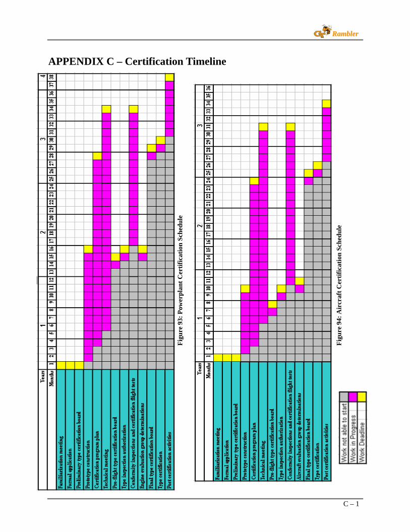
C – 1

RRaammbblleerr

Figu

re 9

3: P

ower

plan

t Cer

tific

atio

n Sc

hedu

le

Figu

re 9

4: A

ircr

aft C

ertif

icat

ion

Sche

dule

APPENDIX C – Certification Timeline

Ref – 1

RRaammbblleerr

References 1 Hanson, Thomas F. A Designer Friendly Handbook of Helicopter Rotor Hubs, 1998. 2 Schrage, Daniel P. Istanbul Technical University-Light Commercial Helicopter Dynamic Analysis of

Rotor System Using Dymore. Georgia Institute of Technology, 2006. 3 Schrage, Daniel P., AE6333 Rotorcraft Design I: Individual and Team Projects, 2005. 4 Kundu, A. K. et al., “Aircraft Component Manufacture Case Studies and Operating Cost Reduction

Benefit,” AIAA 2003-6829, 2003. 5 23rd Annual Student Design Competition, Request for Proposals, “2-Place Turbine Training Helicopter”,

sponsored by AHS International, Inc. and Bell Helicopter, Inc., 2006. 6 Interview conducted with Mr. Blake Moore, Air Atlanta Helicopters, Inc. March 2006. 7 Schrage, Daniel P., “Extension of RF Method to VTOL Aircraft Conceptual and Preliminary Design”,

AE6333 Rotorcraft Design I Course Notes, Georgia Institute of Technology, Fall Semester, 2005. 8 Prouty, Raymond W. Helicopter Performance, Stability and Control. FL: Kreiger, 1995. 9 JVX Technology Assessment, Appendix D – General Parasite Drag Methodology, 1984. 10 PC Based Development, Recurring Production and Operating and Support Cost Model User's Guide,

2001. 11 Leishman, J. Gordon., Principles of Helicopter Aerodynamics, Cambridge University Press, New York,

2000. 12 http://www.flightlab.com. 13 Tapavicza, M. and Och, F., “Application of Damage Tolerance Concepts for MBB Helicopters”,

AGARD Conference Proceedings No. 297. 14 Hanson, Thomas F., “The Auto-Trim Rotor Stability System,” AHS Annual Forum, 1997. 15 Leyes, Richard A., and Fleming, William A., The History of North American Small Gas Turbine

Aircraft Engines. Virginia: AIAA, 1999. 16 Benstein, Eli H., “Small Flying Engines Are Different,” American Institute of Aeronautics and

Astronautics Paper 74-1185, 1974. 17 Aviation Week and Space Technology, (January 17, 2005). 18 Mattingly, Jack D., Heiser, William H., and Pratt, Daniel T., Aircraft Engine Design. 2nd ed. Virginia:

AIAA, 2002. 19 AMCP 706-201 Engineering Design Handbook, “Helicopter Engineering: Part One – Preliminary

Design,” US Army Materiel Command, 1974. 20 Gauntner, James W., “Algorithm for Calculating Turbine Cooling Flow and the Resulting Decrease in

Turbine Efficiency,” NASA Technical Memorandum 81453, (Cleveland, OH: Lewis Research Center, 1980).

21 Clifford, R.J. “Rotating Heat Transfer Investigations on a Multipass Cooling Geometry,” AGARD CP 390, 1985.

22 NEPP User’s Manual, 1997. 23 Japikse, David, and Baines, N.C., Introduction to Turbomachinery. Norwich, VT: Concepts ETI, 1994. 24 “NASA Extended Parametric Representation of Compressor Fans and Turbines,” NASA CR-174646,

Vol. II, General Electric: Cincinnati, OH, 1984. 25Agrawal, M. D. and Bharani, S.. “Performance Evaluation of a Reverse-Flow Gas Turbine Combustor

Using Modified Hydraulic Analogy,” IE Journal. Vol. 85. 2004. 26 Bellocchio, Andrew T. “Drive System Design for a Single Main Rotor Heavy Lift Helicopter,”

Masters Thesis Submitted at Georgia Institute of Technology, 2005. 27 http://www.navygouge.com 28 Langston, Lee S., “Crown Jewels,” Mechanical Engineering Magazine, 2006. 29 Donaldson, Peter. “Power is Control,” Helicopter World (February 1998). 30 http://www.afsfilters.com.

Ref – 2

RRaammbblleerr

31 PC Based Development, Recurring Production and Operating and Support Cost Model User's Guide, 2001.

32 Jackson, K. and Fasnaella, E., “Crashworthy Evaluation of a 1/5 Scale Model Composite Fuselage Section”, NASA/TM-1999-209132 ARL-MR-441, Vehicle Technology Center, Langley Research Center (LARC), Hampton, VA, 1999.

33 Olcott, Dennis D., “Adam Aircraft A500 and A700 Development,” AIAA Presentation, Atlanta, GA, 2006.

34 Tho, C., Sparks C, Smith, Sareen A., and Johnson, C., “Efficient Helicopter Skid Landing Gear Dynamic Drop Simulation Using LS-DYNA,” Bell Helicopter Textron and NAVAIR, American Helicopter Society (AHS) 59th Annual Forum, Phoenix, AZ, May 6-8, 2003.

35 Johnson, Wayne. Helicopter Theory. New York: Dover, 1980. 36 AE 6503 Helicopter Stability and Control Course Notes, Georgia Institute of Technology, Spring Semester, 2006. 37 AE 6070 Rotary Wing Aerodynamics Course Notes, Georgia Institute of Technology, Fall Semester, 2005. 38 Rysdyk, Rolf T. and Calise, Anthony J., “Nonlinear Adaptive Flight Control Using Neural Networks,”

IEEE Controls Systems Magazine, 18 (6):14-25, December 1998. 39 Johnson, E.N. and Mishra, S.S., Flight Simulation for the Development of an Experimental UAV,

Proceedings of the AIAA Modeling and Simulation Technologies Conference, 2002. 40 Schrage, Daniel P. et al., “Application of Software Enabled Control Technologies to a Full-Scale

Unmanned Helicopter,” AIAA Atmospheric Flight Mechanics Conference and Exhibit, San Francisco, CA, 15-18 August 2005.

41 http://www.bluemountainavionics.com/ 42 “Power to Plan is Power to Build” Presentation, Dassault Systemes, 2006. 43 CIMdata, “The Benefits of Digital Engineering,” 2003. 44 US Department of Labor, Bureau of Labor Statistics, Inflation Calculator, http://data.bls.gov/cgi-

bin/cpicalc.pl 45 Systems Engineering Fundamentals, Defense Acquisition University, Fort Belvoir, VA, January 2001. 46 The FAA and Industry Guide to Product Certification, 2nd Ed, 2004.

ahs report georgia tech 2006 - vertical flight society

Documents