ai-based autonomous forest stand generation
TRANSCRIPT
AI-based autonomous forest stand
generation
Using forest stands as key predictor
Diana Saveh
Master thesis
Main field of study: Computer engineer science
Credits: 30hp
Year: 2021
Supervisor: Magnus Eriksson
Examiner: Tingting Zhang
Course code: DT005A
Degree programme: MSE

2
Abstract In recent years, the tech is moving towards a more automized and
smarter software. To achieve smarter software the implementation of AI
is a step towards that goal. The forest industry needs to become more
automized and decrease the manual labor. Decreasing manual labor will
both have a positive impact on both the cost and the environment. After
doing a literature study the conclusion was to use Mask R-CNN to be
able to make the AI learn about the pattern of the different stands. The
different stands were extracted and masked for the Mask R-CNN. First
there was a comparison between the usage of a computer versus Google
Colab, and the results show that Google Colab did deliver the results a
little faster than on the computer. Using a smaller area with fewer stands
gave a better result and decreased the risk of the algorithm crashing.
Using 42 areas with about 10 stands in each gave better results than using
one big area with 3248 stands. Using 42 areas gave the result of an
average IoU of 42%. Comparing this to 6 areas with about 10 stands each
gave the result of 28% IoU. The result of increasing the data split to 70/30
did gave the best IoU with the value of 47%.
Keywords: Forest stands, TensorFlow, AI, QGIS, Mask R-CNN
3
Acknowledgements I would like to thank CGI for the guidance, specifically Magnus Olovsson
for giving me this opportunity, and a huge thanks to Magnus Ericsson at
Mid Sweden University for being a great supervisor. Then I would also
like to thank Elijs Dima at mid Sweden university for great support and
information. Lastly, I would also like to thank TingTing Zhang for being
a great examinator and giving me advice.

4
Table of Contents Abstract ............................................................................................................. 2
Acknowledgements ........................................................................................ 3
Terminology ..................................................................................................... 7
1 Introduction ............................................................................................ 8
1.1 Background and problem motivation ................................................. 8
1.2 Overall aim.............................................................................................. 8
1.3 Problem statement ................................................................................. 9
1.4 Research question .................................................................................. 9
1.5 Scientific goals (Concrete and verifiable) ........................................... 9
1.6 Scope ........................................................................................................ 9
1.7 Outline ..................................................................................................... 9
1.7.1 Contributions ........................................................................................ 10
2 Theory .................................................................................................... 11
2.1 Forest stands ......................................................................................... 11
2.2 QGIS ....................................................................................................... 11
2.3 Machine learning ................................................................................. 12
2.4 Supervised learning ............................................................................. 13
2.5 Computer vision .................................................................................. 14
2.6 Convolutional Neural Networks ....................................................... 14
2.6.1 Object detection .................................................................................... 14
2.6.2 Semantic segmentation ........................................................................ 15
2.6.3 R-CNN.................................................................................................... 15
2.6.4 Fast R-CNN ........................................................................................... 16
2.7 Mask R-CNN ........................................................................................ 16
2.7.1 Loss function ......................................................................................... 17
2.7.2 Intersection over union ........................................................................ 18
2.7.3 Non-Maximum Suppression .............................................................. 18
2.8 Related work ......................................................................................... 18
2.8.1 Mapping roads through deep learning and weakly supervised
training ............................................................................................................ 19
2.8.2 Generating retinal flow maps from structural optical coherence
tomography with artificial intelligence ...................................................... 19
2.8.3 Utilizing Mask R-CNN for Detection and Segmentation of Oral
Diseases ........................................................................................................... 19
2.8.4 Segmentation of Forest to Tree Objects ............................................. 19
2.8.5 Automating Forest stands with Image Segmentation ..................... 20
3 Methodology ........................................................................................ 21
5
3.1 Scientific method description ............................................................. 21
3.1.1 CRISP-DM ............................................................................................. 21
3.2 Business understanding ...................................................................... 22
3.3 Structure the work ............................................................................... 22
3.4 Datamining task ................................................................................... 23
3.5 Evaluate tool ......................................................................................... 23
3.5.1 Comparing R-CNN , Fast R-CNN and Mask R-CNN ..................... 23
3.5.2 Functionality ......................................................................................... 24
3.5.3 Usability and Support .......................................................................... 25
3.5.4 Identify resources ................................................................................. 25
3.6 Data understanding ............................................................................. 25
3.6.1 RGB band ............................................................................................... 26
3.7 Data preparation of TiFF and Shape file .......................................... 27
3.8 Evaluation ............................................................................................. 27
4 Implementation ................................................................................... 28
4.1 Handling the data ................................................................................ 28
4.2 Python .................................................................................................... 29
4.3 How Mask RCNN is used .................................................................. 29
4.3.1 Environment .......................................................................................... 30
4.3.14 Running the Mask R-CNN ........................................................... 30
4.4 Measurement setup ............................................................................. 31
5 Results ................................................................................................... 32
5.1 Manually masking a forest stand ...................................................... 32
5.2 Results of all the areas ......................................................................... 33
5.3 One area ................................................................................................. 35
5.3.1 6 areas ..................................................................................................... 38
5.3.2 42 areas ................................................................................................... 40
6 Discussion ............................................................................................. 43
6.1 Scientific discussion ............................................................................. 43
6.1.1 Manually masking a forest stand ....................................................... 43
6.2 One, six and 42 areas. .......................................................................... 43
6.3 Rpn value loss ....................................................................................... 44
6.4 Project method discussion .................................................................. 45
6.5 Ethical and societal discussion ........................................................... 46
7 Conclusions .......................................................................................... 47
7.1 Project continuation ............................................................................. 47
7.1.1 Computer set against Google Colab .................................................. 47
7.1.2 One big area with many stands versus 6 areas with smaller stands
48
6
7.1.3 Comparing 6 stands versus 42. ........................................................... 48
7.2 Scientific conclusions ........................................................................... 48
7.2.1 Is it possible to create forest stand with the help of ai? .................. 48
7.2.2 Find a good strategy. ............................................................................ 48
7.2.3 How long will it take for the AI to generate results, and will it be
more efficient than traditional methods? ................................................... 49
7.2.4 Compare generated forest stands with manually selected forest
stands. .............................................................................................................. 49
7.2.5 Compare the time and accuracy of forest stand generated in Google
Colab versus forest stands generated on the computer locally. .............. 49
7.2.6 Measure the accuracy. .......................................................................... 50
7.3 Future Work .......................................................................................... 50
Bibliography .................................................................................................. 51
Appendix A: ................................................................................................... 55
7.4 Different stands .................................................................................... 57
7.4.1 6 stands versus one stand on the computer ...................................... 57
7.4.2 6 stands running on computer versus running it on the cloud ..... 60
7.4.3 6 stands on the cloud versus 42 stands on the cloud ...................... 62
7.5 Areas ...................................................................................................... 65
7.5.1 One area ................................................................................................. 65
7.5.2 6 areas ..................................................................................................... 71
7.5.3 42 areas ................................................................................................... 75
7.5.4 42 areas with 70%30% .......................................................................... 76
7
Terminology Acronyms
CNN Convolutional Neural Network
R-CNN Region Convolutional Neural Networks
FCN Fully Convolutional Network
FPN Feature Pyramid Network
CRISP-DM Cross-Industry Standard Practice for Data Mining
RGB Red, Green and Blue
TIFF Tagged Image File Format
ROI Region of Interest
IoU Intersection over Union
8
1 Introduction There is a need for better technology when dividing the forest areas into
different stands. The usage of dividing the forest to different sections is
crucial because cutting down the trees to stimulate new growth makes
the forest healthy. CGI has motivated that if it is possible to generate
forest stands it will be extremely beneficial in the economical aspect.
1.1 Background and problem motivation
Today, traditional methods are used to determine what a forest stands
looks like. A forest stand is an area of the forest that is divided into
different sections.
Traditional methods use airplanes to take pictures of the forest and then
a person has to manually look at these photos to determine
approximately where the forest stand should be. Then the companies in
some instances need to send out people to go to the forest and analyze it,
mainly the height and variety of the trees. They then determine where
the forest stand should be. This is very costly, time-consuming, and
inefficient. Also, the flight photos have a negative impact on the
environment.
1.2 Overall aim
This thesis work will investigate how forest stands can be modernized
with the help of AI/ML. By using modern solutions, the vision is to
generate automated forest stands and to create a more time and cost-
efficient process.
It could be different nature stands and not just forest stands that could
use this modern technology. The parameters could be adjusted to the
specific stand.
The overall aim will be achieved by using Mask R-CNN to generate
forest stands. If this becomes accurate enough then it can replace the old
method i.e. aerial photos and to manually sending out people to look in
the different areas for where these stands should be. This will reduce the
cost by millions according to CGI. This will also be beneficial for the
environment.
9
1.3 Problem statement
The problem with regular that regular forest strand selection is slow and
wasteful, and there does not yet exist an automatic solution. It also cost
a lot for the forest related companies to do this forest stands.
1.4 Research question
The investigated research question of this thesis is to research whether it
is possible to generate forest stands from the coordinates and generate
forest stands based on the training data. What classification accuracy can
be achieved by using location and images in a mask-rcnn predictive
model?
1.5 Scientific goals (Concrete and verifiable)
1. Is it possible to create forest stand with the help of ai?
2. Is it possible to use the location of the forest stand as a parameter
to create and predict new forest stands?
3. How long will it take for the AI to generate this result, and will it
be more efficient than traditional methods?
4. Compare generated forest stands with manually selected forest
stands.
5. Compare the time and accuracy of forest stand generated in
Google Colab versus forest stands generated on the computer
locally.
6. Find a good strategy.
7. Measure the accuracy.
1.6 Scope
The training data will only be focused on the Swedish coordinates for the
forest stand. The rest of the worlds forest stand may differ from the ones
used in this project.
1.7 Outline
Chapter 2 describes the theory of the forest stands and an overview of
machine learning. Then it reveals about convolutional networks and a
literature review.
10
Chapter 3 describes the methodology used in this essay and the tools
used to evaluate it. This is the CRISP-DM and a method from Jose Solarte.
Chapter 4 describes the implementation of the work and how the Mask
R-CNN is used. And more details about the environment and
measurement.
Chapter 5 describes the results of the test conducted on 1,6 and 42 areas.
Graphs over the epoch loss and images of the ground truth and detection
is showcased.
Chapter 6 and 7 discusses results and provides a conclusion.
1.7.1 Contributions
This is a continuation of the Miun project work, the group consisted of
me, Herman Jansson, Lucas Thunberg Wessel and Jawad Ramezanja.
The code that I will be continue using to extract the stands is written by
me and Herman Jansson.

11
2 Theory This chapter is going to explain how the forest industry is operating with
the different forest stands. A deep explanation of the machine learning
required for this project is also given. Then it will describe an overview
of machine learning in general and its components. After that, an
explanation about Convolutional networks is given.
2.1 Forest stands
Forests do contribute to the well being of humans because of its great
properties, which is cleaning the air and giving us useful material that
we can harvest [1]. To preserve and keep the forest as long as possible it
is important to use the knowledge we have about the trees, which is
trimming and diving up the area into different sections.
A forest stand can be defined as “a contiguous group of trees sufficiently
uniform in age-class distribution, composition, and structure, and
growing on a site of sufficiently uniform quality, to be a distinguishable
unit”. [2]
There is no method to model a forest stand but there have been various
methods used. One option is to use a model which include the stand, size
class and tree. They are usually divided into three categories which is to
have specific species, varied-species, same-aged or uneven-aged. [3]
2.2 QGIS
QGIS was created 2002 and is a program where the purpose is for the
user to interact with the data and see it on the maps. QGIS is an open-
source program and is classified as a geographic information system. [4]

12
2.3 Machine learning
To learn something requires different methods such as
exploring/practicing new information and storing the information [5]. To
teach computers is something that has been in the interest for a decade.
The word artificial intelligence was formulated in the 1956 by a man
called John McCarthy which had a presentation about it [6]. After a
couple of years, the first paper about AI that could be acumen and for
example play chess, this article was written by Alan Turning [6] [7].
The thought process behind machine learning was to emulate the human
brain. And in the 1950’s Frank Rosenblatt did create the perceptron
which is used when the dataset is linearly separable. The perceptron is
designed after the neuron of the human brain. The neurons are receiving
and handling the incoming messages. The same thing is happening in the
perceptron. The perceptron handles one or more input and sends out an
output. The perceptron is visualized in the Figure 1. [8]
The numbered x:es is the information receiver, and the circle represents
the place where the input gets processed, which in the computer means
where the calculating takes place. When the input is processed then it
will go to the output where it is written as hθ. [8]
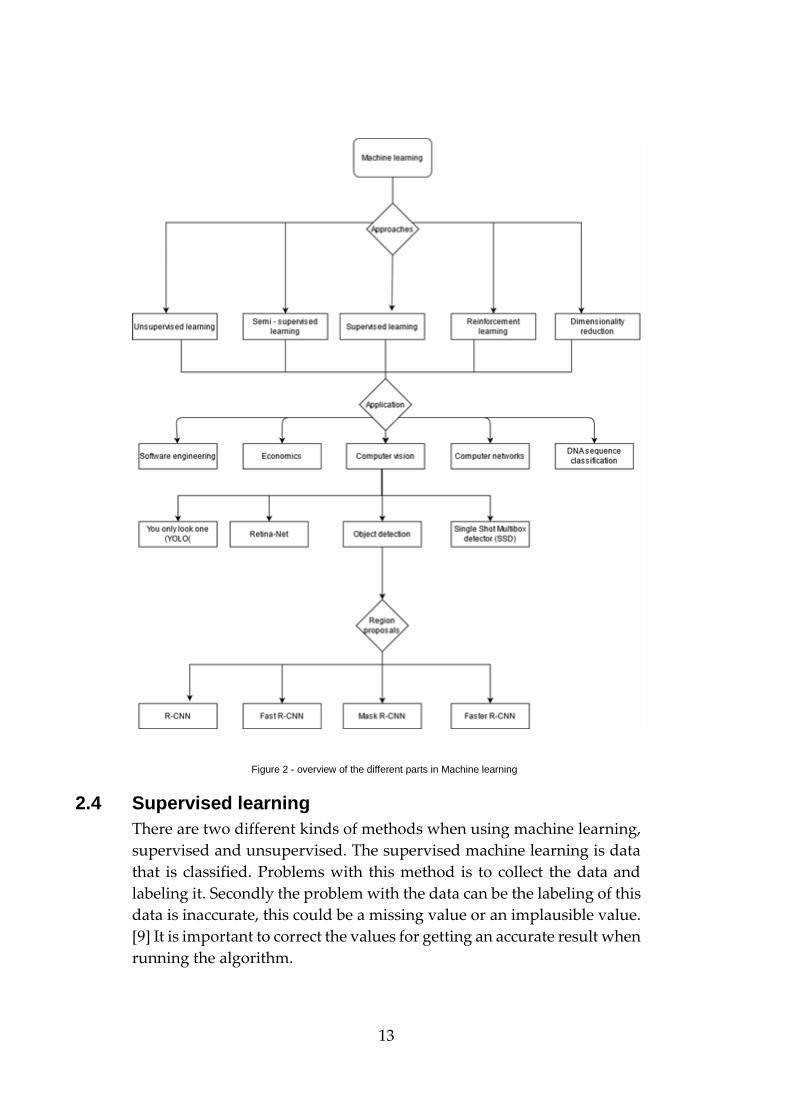
The Figure 2 demonstrates an overview of the different parts of the
different parts of machine learning.
Figure 1 - Perceptron visualized (source: G. Hackeling,
Apply effective learning algorithms to real-world)
13
2.4 Supervised learning
There are two different kinds of methods when using machine learning,
supervised and unsupervised. The supervised machine learning is data
that is classified. Problems with this method is to collect the data and
labeling it. Secondly the problem with the data can be the labeling of this
data is inaccurate, this could be a missing value or an implausible value.
[9] It is important to correct the values for getting an accurate result when
running the algorithm.
Figure 2 - overview of the different parts in Machine learning
14
2.5 Computer vision
Computer vision was developed after the AI was created. Computer
vision was documented to be experimented with in the early 1970s.
Computer vision is as the name suggest the visual aspect. Computer
vision was created to assist in the development of the AI visual aspect, to
try to make a computer recognize what is shown in a picture. This was
developed in MIT. Early computer algorithms were developed to firstly
look at the boundaries of a shape in 2D. [10]
CNN is an algorithm that is used for computer vision, this algorithm is
analyzing the image and extracting data and using it to group the
different patterns and objects together to establish what it is. [11]
2.6 Convolutional Neural Networks
Convolutional networks are mostly used for the visual aspect i.e. image
data. The data is processed, and the AI is finding patterns and
constructing them. [11] [12] CNN has two different approaches which is
the two-stage [13] and one- stage system [14]. Two-stage system is
generating bounding boxes, these groups contain the created candidate
object proposals. The candidates are created in two different steps [15]
[12], while the one-stage technique does the grouping and classification
of the object proposals, all at one time [15].
2.6.1 Object detection
Object detection and image classification had a difference where the
image classification can tell what object is present but not how many,
where object detection could determine how many there are. [12] Object
detection is not limited, it can be used in computer vision, but it is
burdensome when it comes to the background structure and size
difference. [15]Object detection does simply two things, i.e. pinpoints the
units in an image and their position in it. [12]
First step is to do region proposals, which means that you read in the
image and at random and produce bounding boxes. Then an algorithm
is needed to find the optimal place for the box, for example that is the
size of the box, and where on the picture the coordinates for the box
should start and be centered. [12]
15
2.6.2 Semantic segmentation
Segmentation has an input and output, where the input consists of
pictures and the output entail regions and structures. When a picture has
been used it is crucial to treat the image, you treat the image by working
on the filters, gradient, and colour data. [16] Semantic segmentation is
the concept of evaluating every pixel in picture and comprehend it. [16]
[17]
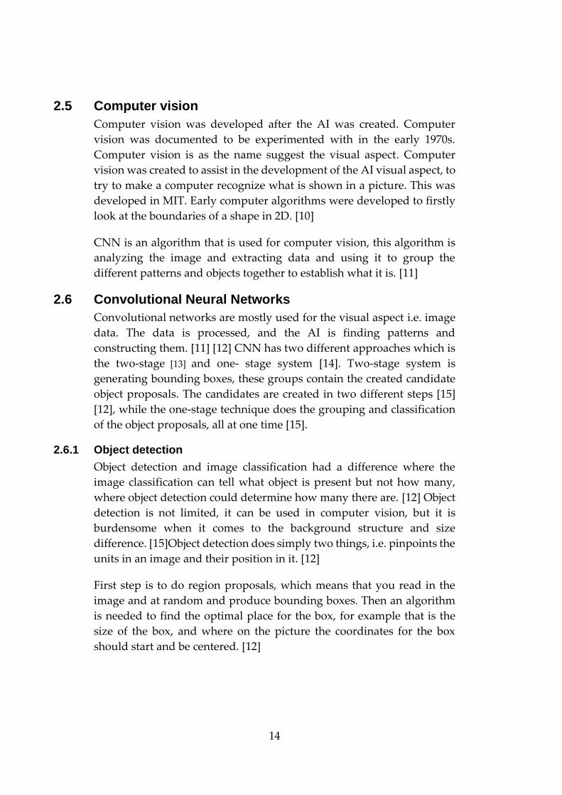
2.6.3 R-CNN
R-CNN stands for “Region based Convolutional Network. R-CNN
begins with analyzing the picture and chooses some areas from it. Within
these areas it tries to identify and label each of these areas. These areas
could be bounding boxes. With the CNN algorithm it does a calculation
to use some of the characteristics of interest and to forecast the
classification. [18]
Figure 3 - R-CNN overview. Source [18]
With R-CNN there are multiple steps of clustering where the clusters gets
bigger. This type of clustering shows that the object does not share the
same size [19]. There are different parts to selective search. The first is
that the selective search is applied on the picture. The selective search
gives the best guess of the areas that would be of interest, and it will
choose them. [20]
After the selective search the data goes through a CNN prior to it
reaching the output layer. [18] The CNN can only handle a small image
that is why the different regions are removed and resized for it. [19]
Thirdly, to instruct the multiple support vector machines for the object
classification, the information that the algorithm has received is united
16
to create a sample for that purpose. Then the bounding box and the
attributes chosen are also united to instruct a linear model for ground-
truth bounding box forecast. [18] That can for example be AlexNet or
VGGNet. A linear model like a support vector machine is used in the
classifier. [19]
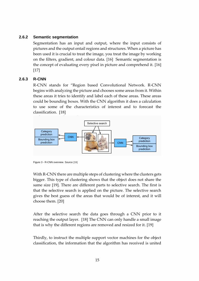
2.6.4 Fast R-CNN
Fast R-CNN is built for the purpose of enhancing the R-CNN. Ross
Girshick made enhancements to the R-CNN because of its slow speed
and memory usage. [21] One of the changes made was removing the
selective search algorithm. Looking at the architecture the input picture
has region proposals, and it is not generated by the Fast R-CNN, the
region proposals is generated beforehand. [22]
In the next step the CNN manages the images and gives the feature map,
the feature map contains the parts of interest and then selected where
they are detected on the image. [22]
Figure 4 - Fast R-CNN architecture. Source [21]
2.7 Mask R-CNN
R-CNN is an abbreviation for Region Convolutional Neural Networks
[15] and the Mask R-CNN is a development of the Fully convolutional
Network (FCN) [17]and fast R-CNN is developed because the difficulty
in instance segmentation.
[17] In instance segmentation there needs to be a more precise
classification, to be even more precise every single pixel is defined with
the object-instance [12],which is called semantic segmentation [17].
17
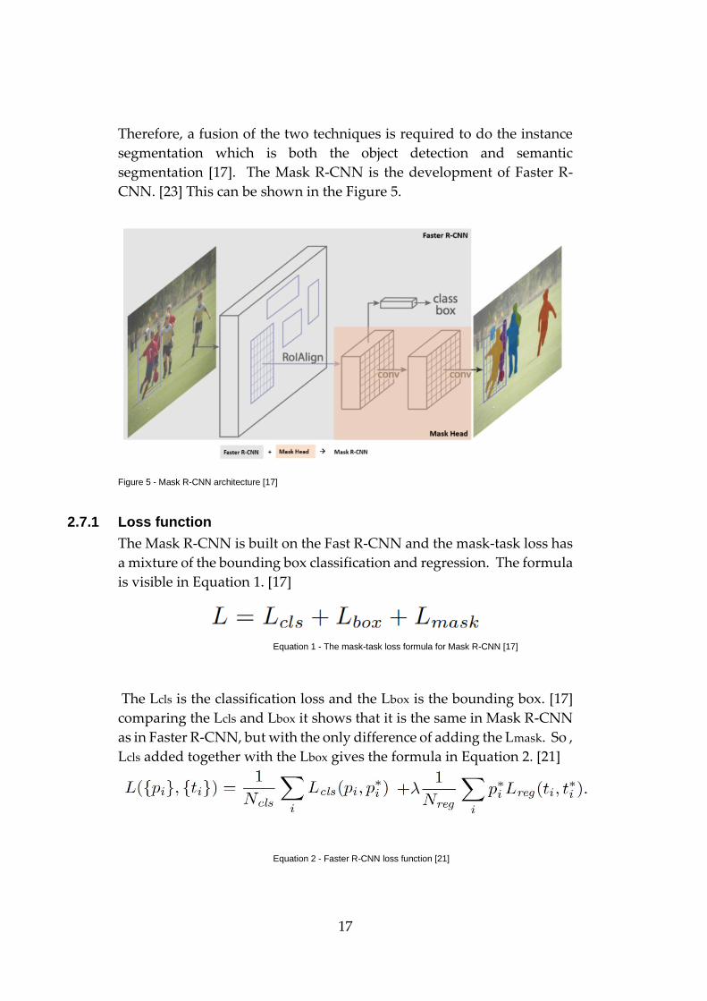
Therefore, a fusion of the two techniques is required to do the instance
segmentation which is both the object detection and semantic
segmentation [17]. The Mask R-CNN is the development of Faster R-
CNN. [23] This can be shown in the Figure 5.
Figure 5 - Mask R-CNN architecture [17]
2.7.1 Loss function
The Mask R-CNN is built on the Fast R-CNN and the mask-task loss has
a mixture of the bounding box classification and regression. The formula
is visible in Equation 1. [17]
Equation 1 - The mask-task loss formula for Mask R-CNN [17]
The Lcls is the classification loss and the Lbox is the bounding box. [17]
comparing the Lcls and Lbox it shows that it is the same in Mask R-CNN
as in Faster R-CNN, but with the only difference of adding the Lmask. So ,
Lcls added together with the Lbox gives the formula in Equation 2. [21]
Equation 2 - Faster R-CNN loss function [21]
18
The output of the Lmask is Km², and in the essay written by [17] says
that the K stands for the binary masks with the resolution of m x m,
which means that is the number of K classes.
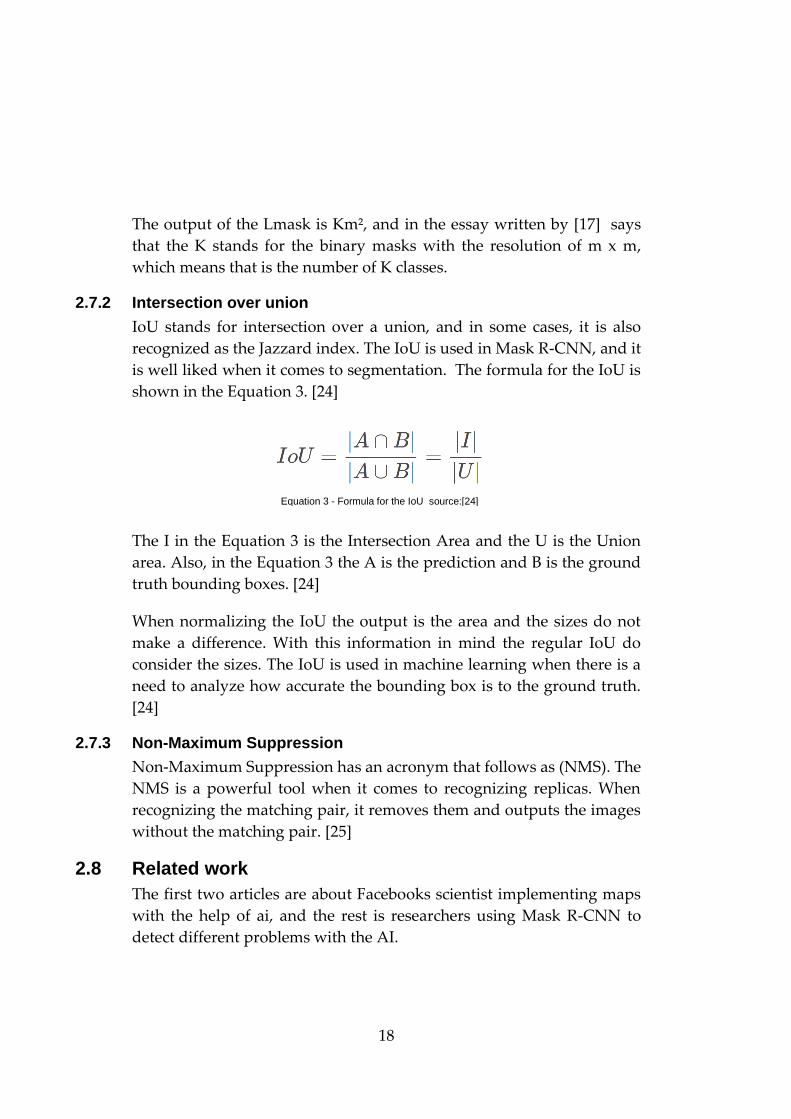
2.7.2 Intersection over union
IoU stands for intersection over a union, and in some cases, it is also
recognized as the Jazzard index. The IoU is used in Mask R-CNN, and it
is well liked when it comes to segmentation. The formula for the IoU is
shown in the Equation 3. [24]
The I in the Equation 3 is the Intersection Area and the U is the Union
area. Also, in the Equation 3 the A is the prediction and B is the ground
truth bounding boxes. [24]
When normalizing the IoU the output is the area and the sizes do not
make a difference. With this information in mind the regular IoU do
consider the sizes. The IoU is used in machine learning when there is a
need to analyze how accurate the bounding box is to the ground truth.
[24]
2.7.3 Non-Maximum Suppression
Non-Maximum Suppression has an acronym that follows as (NMS). The
NMS is a powerful tool when it comes to recognizing replicas. When
recognizing the matching pair, it removes them and outputs the images
without the matching pair. [25]
2.8 Related work
The first two articles are about Facebooks scientist implementing maps
with the help of ai, and the rest is researchers using Mask R-CNN to
detect different problems with the AI.
Equation 3 - Formula for the IoU source:[24]

19
2.8.1 Mapping roads through deep learning and weakly supervised training
Researchers at the Facebook AI department uses AI to draw maps where
the maps are not accurate or nonexistent, according to the researchers
they used a weak supervised training to guess different parts of the map.
For completing the maps satellite images were used, in a test they did
use training data from the entire country which predicted accurate
results in Thailand but using the same training data in other countries
did not produce the same result. [26]
2.8.2 Generating retinal flow maps from structural optical coherence tomography with artificial intelligence
This article is related because the scientist uses retinal flow maps to train
an AI and then uses this flow maps to deviate from using professional
help to classify the retina flow maps. The approach that was used by the
scientist is that their dataset was separated into training and validation
and a held-out test, the percentage of this training was split between
70%15%15%. They also explain that the most suitable parameter was
used. The scientist also tested 12 different deep learning models and the
function used for training the data was the adam learning function. [27]
2.8.3 Utilizing Mask R-CNN for Detection and Segmentation of Oral Diseases
In this paper the researchers use Mask R-CNN which was based on
Matterport Inc code (https://github.com/matterport/Mask
RCNN), they limit the research to only use it for identifying the highly
widespread disease in oral pathology which is herpes labialis and
aphthous ulcer. They compared the result to another pixelwise classifier
in the same area and found out that their model had a higher
accuracy .744 vs .621 even though the latter had 258 images and their
only had 30 images. They hypothesize that it would have been a better
result if they had been able to have more images to use as data, and
they did prove that with this algorithm the accuracy will be higher even
with less data provided. [28]
2.8.4 Segmentation of Forest to Tree Objects
In this essay they research if it is possible to do a segmentation using only
the height of trees as the data. They use the raster data. The data needed
to be separated because some of the LiDAR data containing some
variations and the irrelevant branches get removed.

20
LiDAR data is used to analyze the maximum and smallest reflection in a
pixel. And they do loose some of the information of the data, but this is
done so that the program would be running faster to decrease the
computational power required. [29]
2.8.5 Automating Forest stands with Image Segmentation
This work is a continuation of the work I did in a group. In the group we
used GAN to try to identify the different stands. When using GAN the
problem was that the algorithm went into a mode collapse. The solution
was using object segmentation algorithms, but the problem was that it
was not an ai, so there was not a learning process. [30]
21
3 Methodology This chapter discussed the methodology used in this essay. One
important aspect of this report was handling a lot of data because every
stand took space, all of the data of Sweden was 13GB (before dividing it
up). When handling a lot of data, it was important to carefully do so, or
else there could be an error when running it through the Mask R-CNN.
The methodology used to help in this process was a mixture of CRISP-
DM and a methodology proposed by Jose Solarte, which had a more
detailed approach on how to tackle a datamining task. Some parts of the
methodology steps are focused on the evaluation of the project with the
goal of delivering a product. Since this project had no intention of that,
those parts of the methodology were discarded.
3.1 Scientific method description
I used a quantitative method to measure the accuracy of the project. The
comparisons are numerical. I did experiments and measured the
accuracy and time. Gantt was used to keep the work on track. Gantt is a
schedule technique which gives the user the ability to keep the work
trackable and to do every single task that is needed to be able to complete
before the deadline.
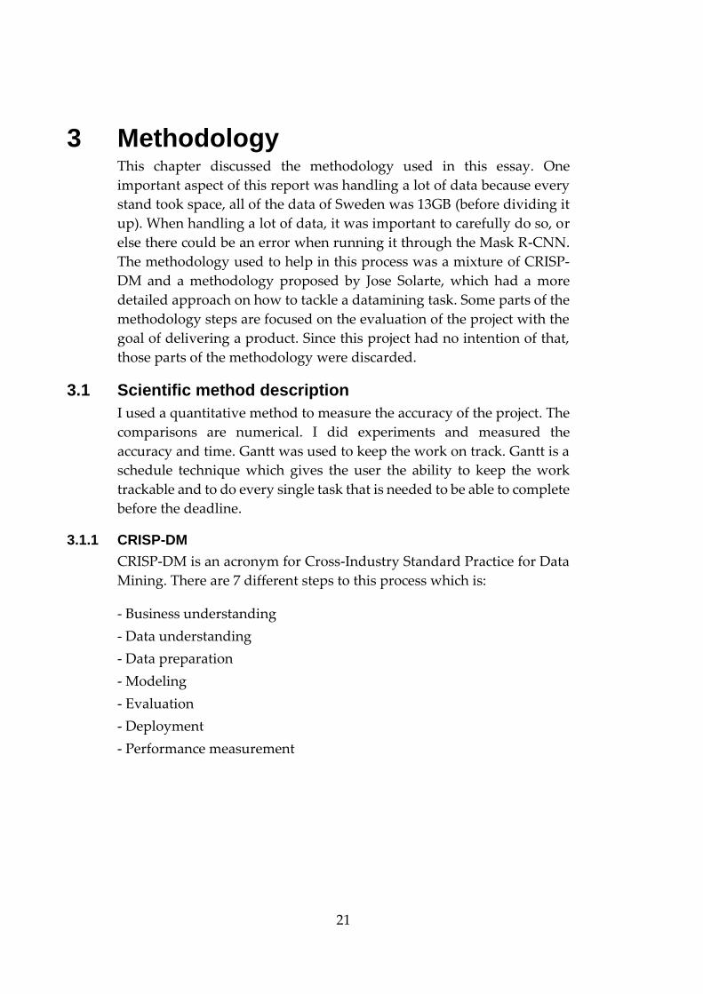
3.1.1 CRISP-DM
CRISP-DM is an acronym for Cross-Industry Standard Practice for Data
Mining. There are 7 different steps to this process which is:
- Business understanding
- Data understanding
- Data preparation
- Modeling
- Evaluation
- Deployment
- Performance measurement
22
Figure 6 - Crisp DM process source: [31]
The method used was CRISP-DM and a proposed method from Jose
Solarte where the methodology was very detailed, it was based on
CRISP-DM and SEMMA. However, Solartes method was proposed for
students in industrial engineering which is why the economic
perspective was not used and the focus was on the data mining and
analyzing the data. [32]
3.2 Business understanding
First the business understanding (the first step) was analyzed for the
organization which was CGI in this particular case. CGI needed a
solution for their forest stand problem. The solution which CGI wanted
solved was to make the forest stand automatically. Details of this was
written in chapter 1 and 2.
3.3 Structure the work
After the business understanding the work needed to become more
structured and some information about the forest stand was needed,
hence a literature study was conducted. The literature study was
conducted to understand what algorithm, and how to structure the data
is the most appropriate for the task. The essay did follow the proposed
methodology of Solarte [32] which was choosing between the following:
-Description and summarization
- Segmentation
23
-Concept description
-Classification
-Prediction
-Department analysis
An example of this process is found in Figure 6 [31]
The segmentation step was picked after doing the literature study for the
essay. There was an experiment [33] that used Mask-RCNN on nucleus
data, and after reading about that and how the Mask-RCNN the
segmentation looked promising.
3.4 Datamining task
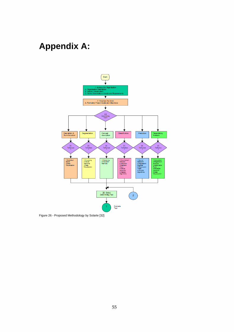
According to the figure in Appendix A: Figure 26 there was a need for an
analyzation of the datamining task. When doing the analyzing the forest
stands showed a need to use segmentation. The segmentation was
necessary because the stands needed to be separated and analyzed by the
algorithm in order to find a pattern for the different stands.
The next step in Appendix A: Figure 26 was to find the technique that
was needed, the technique used was neural network because the
algorithm required it to be trained with the aim of finding patterns.
3.5 Evaluate tool
To evaluate the algorithm chosen the use of Appendix A: Figure 26
guided through the different areas that needed to be inspected.
Doing the literature study, it pointed to an algorithm called Mask R-CNN.
This algorithm did solve the segmentation of the forest stands. The Mask
R-CNN algorithm was able to run locally on the computer, the
specification of the computer is shown in Table 1.
3.5.1 Comparing R-CNN , Fast R-CNN and Mask R-CNN
Comparing the Mask R-CNN to R-CNN, Fast R-CNN and Faster R-CNN
the Mask R-CNN is superior.
The limitation of the R-CNN was the speed [18], when training the data
there was multiple steps in the process. Because of these multiple steps,
the training took time, and needed a decent computer to be able to do the

24
calculations. Also, a lot of space was required because every object
proposal in the data was written to the computer’s storage unit. [21] R-
CNN had a slow speed hence why it is not used a lot. [18]
Lastly the negative part of R-CNN was that the object detection was not
as fast as it could be when trained with the VGG16 network. The
conclusion was that it takes 47 seconds for every picture. [21]
Comparing the Fast-RCNN and R-CNN the difference was that Fast R-
CNN is 9 times faster when it came to training. When comparing the time
spent running the models, it was 213 times faster than R-CNN. Also, it
had a considerable better score on the mAP on the Pascal VOC 2012
dataset. [12]
Figure 7 - comparison of R-CNN and Fast R-CNN Source: [21]
Mask R-CNN was a more precise object detector than faster R-CNN.
[23]The overhead generated by Mask R-CNN was very minuscule
because the algorithm uses the already present network. Because of this
small overhead the processing is practically the same as Faster R-CNN.
[12]
3.5.2 Functionality
The Mask R-CNN had a good set of functionalities. One of the many
good features was that it was possible to train different layers, for
example if there was an error when running all layers, there was a
possibility to divide the layers and begin with only training the head
layer. Dividing the layers was necessary in the beginning of the work, on
25
the first run of the algorithm because when running all the layers in the
beginning it crashed. This helped for analyzing how to input correct
parameters for the Mask R-CNN.
When training the Mask R-CNN , another neat functionality was that
there was a possibility to continue to train an already trained model,
which I did use. One example is when there was more data available. So
instead of creating a new model from scratch, it was possible to take a
previously trained model and continue to train it with the new data. This
functionality was very useful and saved a lot of time and computing
power.
3.5.3 Usability and Support
Since the purpose of this work was not to create, nor evaluate a tool in
terms of usability, the usability, and the support of Mask-RCNN was not
considered. The focus had been towards the functionality, to make sure
the proper tests/training and analyzation of the result could be
performed in a good manner.
3.5.4 Identify resources
The next part of the process was about making sure that the project was
feasible, in short, to determine if the project could be executed or not. The
steps were to identify the resources required by the tool, determine
additional required resources and from that, decide if the project was
feasible. The resources required by Mask-RCNN was the training and
test-data, along with an environment that had sufficient memory to load
the data necessary to perform the training.
3.6 Data understanding
The next step was to gather all the data, prepare the data and then run
that through the machine learning algorithm. In this report the data
collected was the different stands of the different areas of forests. The
preparation consisted of randomly selecting smaller areas and dividing
them into test and training. Then all the different stands in those areas
was first extracted and then masked, so the Mask R-CNN had a ground
truth. All the training data was then fed into the Mask R-CNN during the
training phase.
The parameters available was:
- Height

26
- Tree species
- Vegetation
- Volume (m3sk / ha)
- Manually selected forest stands.
3.6.1 RGB band
The data consisted of three bands, RGB which stands for red, green and
blue. These different colors represent different data. The data in the
report these colors were representing different aspects of the trees, in this
case the red stood for the height of the trees. The height was especially
important to know because a huge part of dividing the forest stands did
depend on the height of the trees.
The green band was the basal area, and it told how much trees there were
in the area. The basal area was measured by taking the height of 1.3m of
the ground, and with a diameter of the tree’s circumference was
measured. [34] The formula for measuring the basal area was written as:
𝐵𝐴 =𝜋 𝑥 𝑑𝑏ℎ2
40000
Equation 4 – Basal area equation
The basal area was measured in sq m. The dbh was a shortening for
“diameter at breast height” in cm which was around 1.3 m [34] from the
ground. The areas of all trees could be used as a measurement to see how
crowded the stand was. This measurement was called the basal area of
a stand. [35]
The blue band stood for the volume. The volume was calculated in m3 by
using the mid-point diameter and size of every tree. There were two
different conditions that needed to be fulfilled when measuring trees.
The one that was fulfilled first was the one that was used. The first
condition was if the overbark was 7 cm then that was used (trees at breast
height with a lesser diameter than 7 cm were routinely disregarded). The
second condition was when the main stem was distinct. [35]
To estimate the volume there was different methods, but one method
was using the following equation:
27
𝑉 = (𝐵𝐴
2+ 0.0019) 𝑥 𝐻
Equation 5 – Volume of trees formula in m3
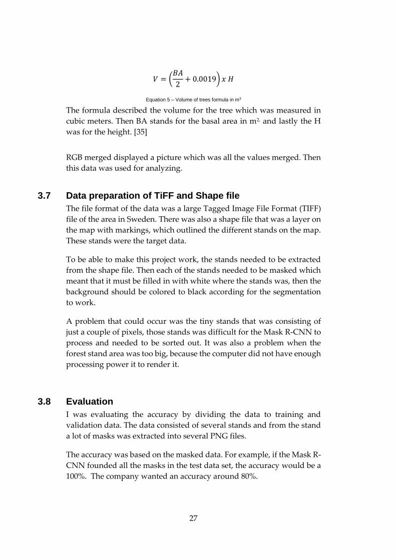
The formula described the volume for the tree which was measured in
cubic meters. Then BA stands for the basal area in m2, and lastly the H
was for the height. [35]
RGB merged displayed a picture which was all the values merged. Then
this data was used for analyzing.
3.7 Data preparation of TiFF and Shape file
The file format of the data was a large Tagged Image File Format (TIFF)
file of the area in Sweden. There was also a shape file that was a layer on
the map with markings, which outlined the different stands on the map.
These stands were the target data.
To be able to make this project work, the stands needed to be extracted
from the shape file. Then each of the stands needed to be masked which
meant that it must be filled in with white where the stands was, then the
background should be colored to black according for the segmentation
to work.
A problem that could occur was the tiny stands that was consisting of
just a couple of pixels, those stands was difficult for the Mask R-CNN to
process and needed to be sorted out. It was also a problem when the
forest stand area was too big, because the computer did not have enough
processing power it to render it.
3.8 Evaluation
I was evaluating the accuracy by dividing the data to training and
validation data. The data consisted of several stands and from the stand
a lot of masks was extracted into several PNG files.
The accuracy was based on the masked data. For example, if the Mask R-
CNN founded all the masks in the test data set, the accuracy would be a
100%. The company wanted an accuracy around 80%.

28
4 Implementation This chapter showcased a flowchart of how the areas got extracted and
used in the Mask R-CNN. The programming language python was
chosen, and a description of how Mask R-CNN was used with the setup
was described.
4.1 Handling the data
There were different steps to train the
Mask RCNN. These steps were
demonstrated in Figure 8.
Firstly, the extraction was executed by
different steps. First step was to extract an
area. Dividing the data was important
because of the computers processing time.
If an area was not extracted, then the
processing would be too big for the
computer to handle.
Secondly, an area of choice was selected,
and in this report, it was an area in the
south of Sweden. There was a TIFF file and
a shape file for the area. The shape layer
was used to extract the different stands
from the selected area. These stands were
selected, and an extraction was made from
the area.
Thirdly the images were converted to a
different format. This format was crucial
because the input of the Mask-RCNN only
accepted PNG files.
Furthermore, the images were masked. The masking was a process
where the stands that were on the area was extracted in order to teach
the algorithm where the different stands were. With this in mind there
was not a possibility to input more than one stand at a time into the
algorithm, the different stands on the picture needed to separately be
inputted to teach the algorithm the different stands. In the masked image
Figure 8 - flowchart of the data
29
the stand was filled in with a white color then the rest of the picture was
filled in with black. Then a new picture was created and the stand next
to the previous one was chosen.
The first approach for masking the pictures were made in adobe
photoshop. The next step was doing it automatically.
With atomization the data was filled in using code. The code did analyze
each pixel, if the pixel contained a color, then it was colored white. If
there was not any color, then it was set to black. The black was created
by using the RGB colors in the picture and setting them to the values
0(0,0,0) and the stand was colored in by setting the RGB to white which
is the number 255 (255,255,255).
Lastly the data was then used as an input in the Mask R-CNN. All of the
data was split into two parts, one was the training data, and was the
validation data. The data sent into the algorithm was the TiFF file
converted to png and masked images for each stand.
4.2 Python
The code was written in python. Python is a programming language
which was widely used for machine learning. A benefit of using python
was that it was focused on readability which made it easy to read, and
they also did reinforce modules and packages. [36]
4.3 How Mask RCNN is used
The Mask R-CNN implementation was based on the foundation made
from matterports code from github. The code used was tested on
microscopic images. [37]
When running the Mask R-CNN it requires a set of weights. The weights
used in this paper was by MS-COCO. The MS-COCO weights were a
pretrained model which made it easier when training a new dataset for
the first time.
When training a Mask-RCNN model, it was possible to specify which
layers to train. The user could either train all layers, a choice of layers or
select a predefined setting, called heads. The layer that was going to be
trained was specified. The purpose of using heads was basically to keep
the training time down when the data was trained on. Similar to the data
30
that the model had trained on previously. When using the heads setting
only the RPN (Region Proposal Network), the FPN (Feature Pyramid
Network) and mask heads of the network was trained. [17]
RPN is a neural network that proposed what regions in an image might
contain the objects that were being looked after, also called ROI (Region
Of Interest). That way, the rest of the layers would not have to scan the
whole areas but can instead focus on the areas that had been proposed
by the RPN. [17]
FPN is, very simplified, a CNN with the purpose of trying to identify the
objects searched for in different scales that may occur in the image. When
searching for a forest stand it did find a small stand as well as a stand
that might cover a quarter of the image. [38]
Also, the Mask head would be trained which was responsible to mask all
the ROIs that had been identified in the previous steps.
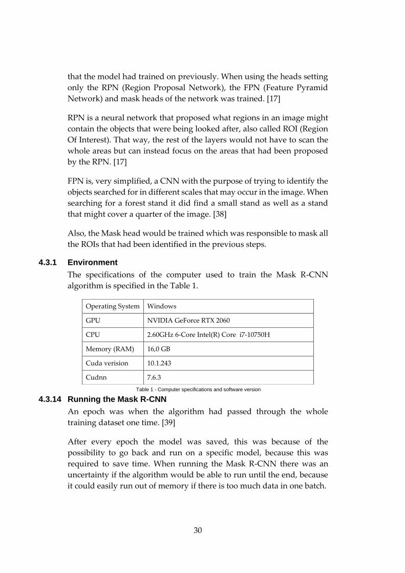
4.3.1 Environment
The specifications of the computer used to train the Mask R-CNN
algorithm is specified in the Table 1.
Table 1 - Computer specifications and software version
4.3.14 Running the Mask R-CNN
An epoch was when the algorithm had passed through the whole
training dataset one time. [39]
After every epoch the model was saved, this was because of the
possibility to go back and run on a specific model, because this was
required to save time. When running the Mask R-CNN there was an
uncertainty if the algorithm would be able to run until the end, because
it could easily run out of memory if there is too much data in one batch.
4.3.2 Operating System 4.3.3 Windows
4.3.4 GPU 4.3.5 NVIDIA GeForce RTX 2060
4.3.6 CPU 4.3.7 2.60GHz 6-Core Intel(R) Core i7-10750H
4.3.8 Memory (RAM) 4.3.9 16,0 GB
4.3.10 Cuda verision 4.3.11 10.1.243
4.3.12 Cudnn 4.3.13 7.6.3
31
4.4 Measurement setup
Along with the model there was logs in the file which gave the possibility
to use Tensorboard for analysing the data. The model file was saved as
a .h5 file which contained the trained model along with a timestamp. The
timestamp was from when the epoch was finished running.
In Tensorboard the information given was epoch loss i.e adding the
following losses: RPN classifier loss, RPN bounding box loss graph, loss
for the classifier head of the Mask R-CNN, loss for the Mask R-CNN
bounding box and lastly mask binary cross-entropy loss for the mask
head.
32
5 Results The manually extracted stands data was not sufficient for it to be able to
run, because it did not have enough stands. When using code to run the
masking, the masking was made in an instant which is necessary when
working with a lot of training data.
Firstly, the big area with 3248 stands did take 2 days to run and was on
the verge of running out of memory. Secondly the areas were extracted
with a smaller number of stands. That made a big difference when it
came to the memory on both the computer and Google Colab, both
platforms managed to run the algorithm smoothly.
When the algorithm was done running, the log file was saved. Then the
log file was used to run the analyzing section, which was provided by
Matterport Inc [37]. The code contained a Jupiter notebook. The Jupiter
notebook helped to investigate the dataset, running statistics on it and
analyze the detection from the beginning to the end.
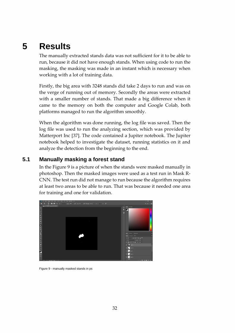
5.1 Manually masking a forest stand
In the Figure 9 is a picture of when the stands were masked manually in
photoshop. Then the masked images were used as a test run in Mask R-
CNN. The test run did not manage to run because the algorithm requires
at least two areas to be able to run. That was because it needed one area
for training and one for validation.
Figure 9 - manually masked stands in ps

33
5.2 Results of all the areas
The epoch loss of the areas 1, 6 and 42 is visible in Figure 10. The epoch
loss was all of the different losses added together. The different losses
were the RPN classifier loss, RPN bounding box loss graph, loss for the
classifier head of the Mask R-CNN, loss for the Mask R-CNN bounding
box and lastly mask binary cross-entropy loss for the mask head.
Figure 10 - Comparison of all the different areas
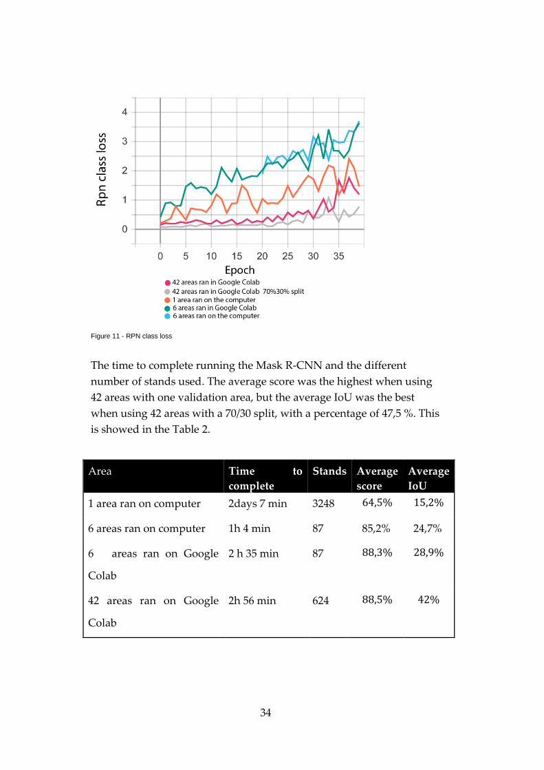
The RPN class loss, which was the RPN anchor classifier loss, is visible
in the Figure 11. The RPN was the region of proposal network, and it
displayed the classification loss, which signifies the belief in forecasting
the class labels.
34
Figure 11 - RPN class loss
The time to complete running the Mask R-CNN and the different
number of stands used. The average score was the highest when using
42 areas with one validation area, but the average IoU was the best
when using 42 areas with a 70/30 split, with a percentage of 47,5 %. This
is showed in the Table 2.
Area Time to
complete
Stands Average
score
Average
IoU
1 area ran on computer 2days 7 min 3248 64,5% 15,2%
6 areas ran on computer 1h 4 min 87 85,2% 24,7%
6 areas ran on Google
Colab
2 h 35 min 87 88,3% 28,9%
42 areas ran on Google
Colab
2h 56 min 624 88,5% 42%
35
42 areas ran on Google
Colab with 70%30% split
2h 51 min 624 86,9% 47,5%
Table 2 - Time to complete running the stands with different number of areas and Average score and IoU from all the
different areas
5.3 One area
The one big area was the most difficult to run because of the size of the
area and the amount of stands in it. The total amount of stands in this
area was 3248.
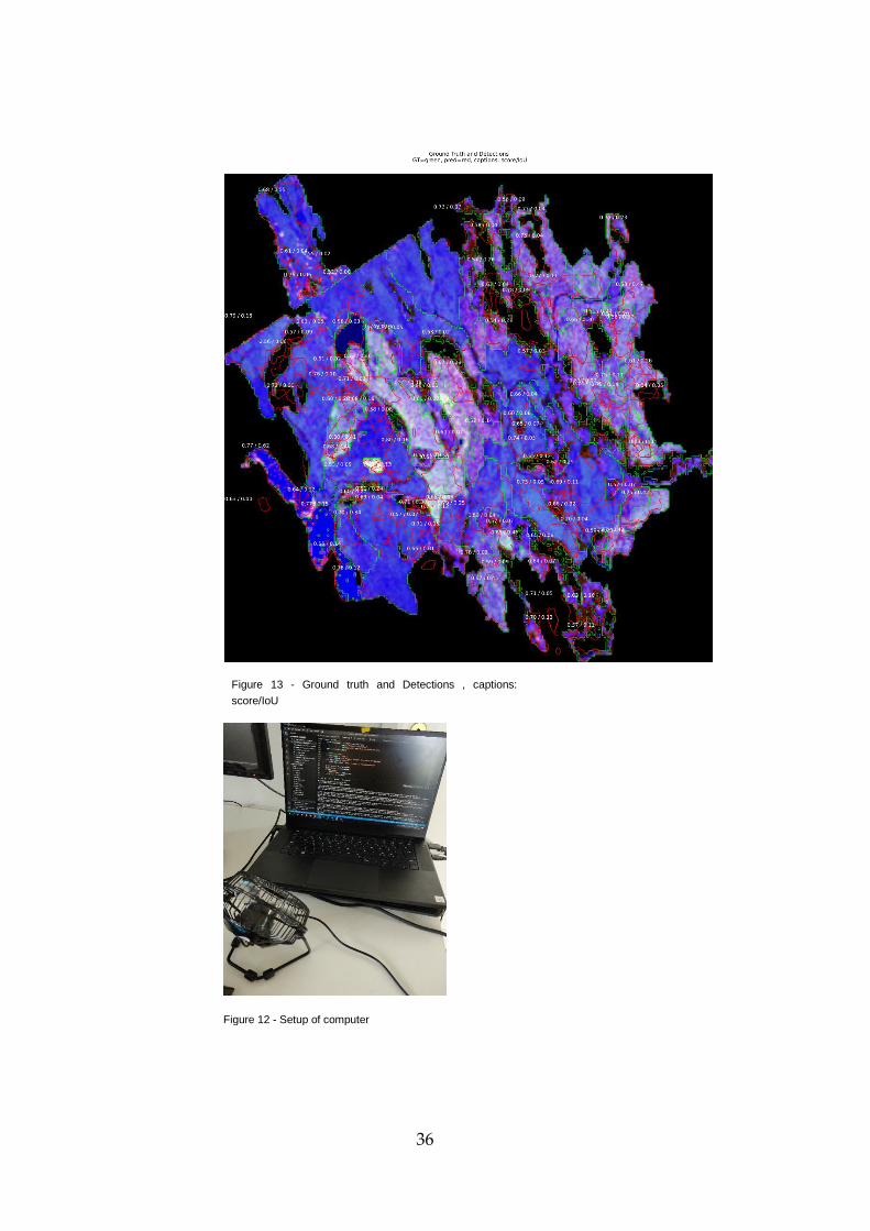
The setup of my environment was a laptop and a fan beneath it, and also
a mini-fan on the front to prevent the computer of overheating when it
ran for two days, this can be seen in Figure 12.
The computer did manage to run out of memory many times, with a
strike of luck, it worked. But it did not manage to run again which
indicates that it was on the edge of working and not working. This was
tested both on Google Colab and locally on the computer. The only time
it did not run out of memory was on the computer. Because of its massive
size of 3248 stands it did take a long time to run, a total of two days to be
exact. This can be seen in Table 2.
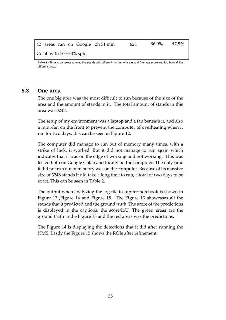
The output when analyzing the log file in Jupiter notebook is shown in
Figure 13 ,Figure 14 and Figure 15. The Figure 13 showcases all the
stands that it predicted and the ground truth. The score of the predictions
is displayed in the captions: the score/IoU. The green areas are the
ground truth in the Figure 13 and the red areas was the predictions.
The Figure 14 is displaying the detections that it did after running the
NMS. Lastly the Figure 15 shows the ROIs after refinement.
36
Figure 12 - Setup of computer
Figure 13 - Ground truth and Detections , captions:
score/IoU

37
Figure 15 - Detections after NMS
Figure 14 - ROIs after refinement
38
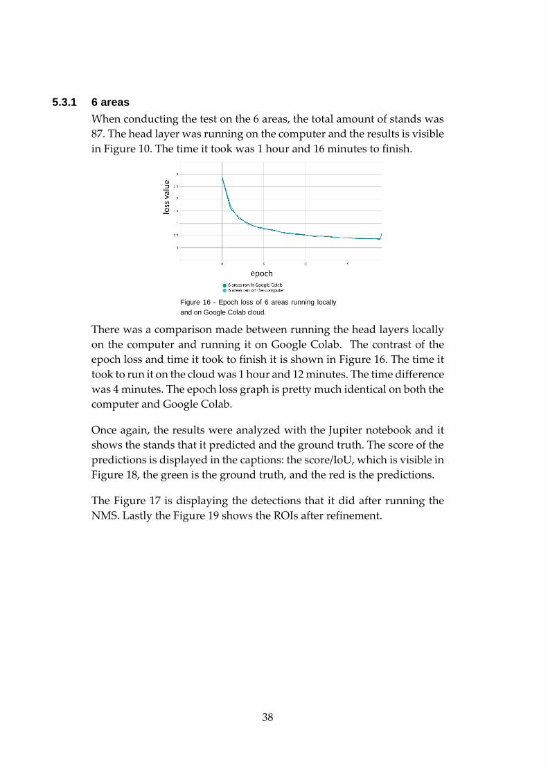
5.3.1 6 areas
When conducting the test on the 6 areas, the total amount of stands was
87. The head layer was running on the computer and the results is visible
in Figure 10. The time it took was 1 hour and 16 minutes to finish.
There was a comparison made between running the head layers locally
on the computer and running it on Google Colab. The contrast of the
epoch loss and time it took to finish it is shown in Figure 16. The time it
took to run it on the cloud was 1 hour and 12 minutes. The time difference
was 4 minutes. The epoch loss graph is pretty much identical on both the
computer and Google Colab.
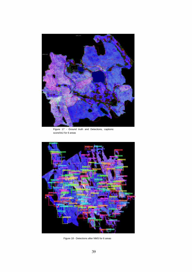
Once again, the results were analyzed with the Jupiter notebook and it
shows the stands that it predicted and the ground truth. The score of the
predictions is displayed in the captions: the score/IoU, which is visible in
Figure 18, the green is the ground truth, and the red is the predictions.
The Figure 17 is displaying the detections that it did after running the
NMS. Lastly the Figure 19 shows the ROIs after refinement.
Figure 16 - Epoch loss of 6 areas running locally
and on Google Colab cloud.
39
Figure 17 - Ground truth and Detections, captions:
score/IoU for 6 areas
Figure 18 - Detections after NMS for 6 areas

40
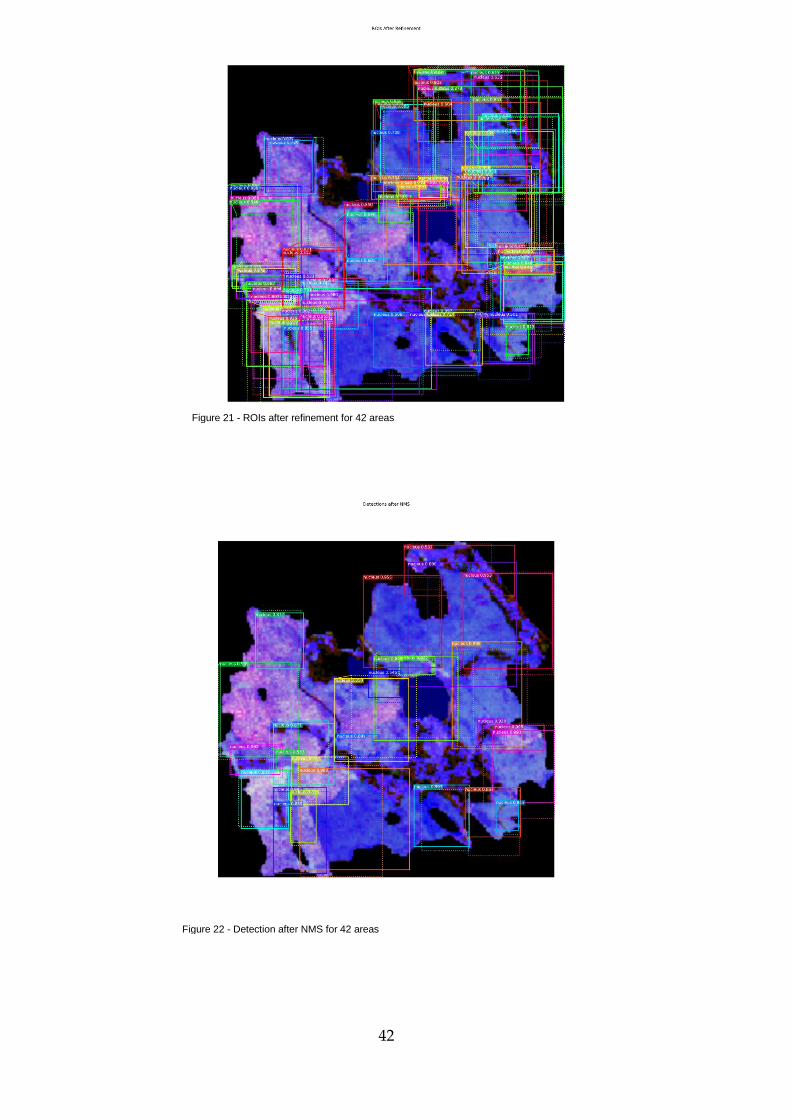
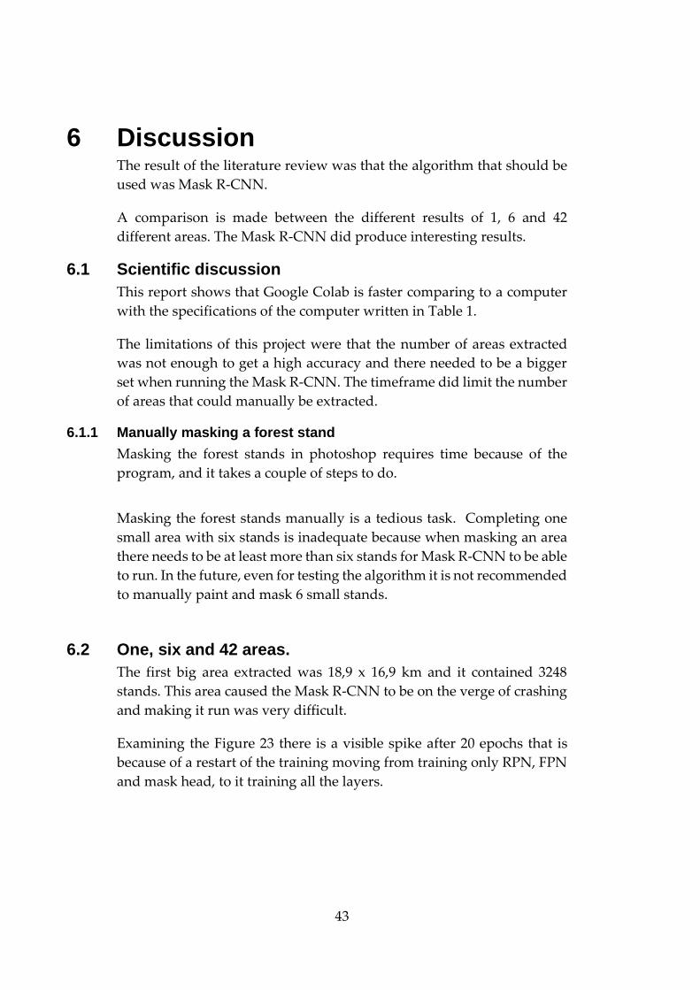
5.3.2 42 areas
The 42 areas result of epoch loss and time is visible in the Figure 10, and
the time it took to finish it was 2 hours and 56 minutes. The amount of
stands in the 42 areas were 624.
Once again, the ground truth and the algorithm predictions are visible
on the Figure 20 and the score of the predictions is displayed in the
captions: the score/IoU, where the green is the ground truth and the red
is the predictions.
The Figure 22 is displaying the detections that it did after running the
NMS. Lastly the Figure 21 shows the ROI after refinement.
Figure 19 - ROIs after refinement for 6 areas

41
Figure 20 - Ground truth and Detections, captions:
score/IoU for 42 areas
42
Figure 21 - ROIs after refinement for 42 areas
Figure 22 - Detection after NMS for 42 areas
43
6 Discussion The result of the literature review was that the algorithm that should be
used was Mask R-CNN.
A comparison is made between the different results of 1, 6 and 42
different areas. The Mask R-CNN did produce interesting results.
6.1 Scientific discussion
This report shows that Google Colab is faster comparing to a computer
with the specifications of the computer written in Table 1.
The limitations of this project were that the number of areas extracted
was not enough to get a high accuracy and there needed to be a bigger
set when running the Mask R-CNN. The timeframe did limit the number
of areas that could manually be extracted.
6.1.1 Manually masking a forest stand
Masking the forest stands in photoshop requires time because of the
program, and it takes a couple of steps to do.
Masking the forest stands manually is a tedious task. Completing one
small area with six stands is inadequate because when masking an area
there needs to be at least more than six stands for Mask R-CNN to be able
to run. In the future, even for testing the algorithm it is not recommended
to manually paint and mask 6 small stands.
6.2 One, six and 42 areas.
The first big area extracted was 18,9 x 16,9 km and it contained 3248
stands. This area caused the Mask R-CNN to be on the verge of crashing
and making it run was very difficult.
Examining the Figure 23 there is a visible spike after 20 epochs that is
because of a restart of the training moving from training only RPN, FPN
and mask head, to it training all the layers.

44
The graph in Figure 23 (the highlighted areas) indicates that it has not
really flattened out, so this model is still a little underfitted. It seems to
be moving towards a good fit which indicates a better predicting model.
If it would continue training it probably would have resulted in a good
fit.
Every graph that has to do with the validation data looks different than
the average validation data. The reason for it to look different may be
due to the validation set being set too small.
In Table 2 the score is a confidence score for the prediction. I.e. a high
confidence score means that the model is confident that the marked area
is a stand. Looking at the average of the IoU, the best average IoU is the
42 areas with a data split of 70/30. The 70/30 split means that 70% is
training data and the 30 % is the validation data, and in this case the
validation was 12 stands. The result it gave was an IoU of 47,5%. The
IoU is pretty decent and with only 624 stands it was better than expected.
To be able to get a high IoU there needs to be more automatization when
it comes to extracting the areas with the stands in it, that is to make it
possible to get a bigger training set without having to spend a lot of time
on just the extraction of the stands.
6.3 Rpn value loss
Analyzing the graphs given from the results in Figure 10, there is a more
stable line in the training and validation split where it has a 70/30 split
Figure 23 - highlighted area shows stabilization.

45
instead of using only one area as a validation. The Figure 24 is a zoomed
figure from the results in the Figure 11.
The reason for the values changing more rapidly is, when a small change
is made to make the model better, a bigger impact is visible in the graphs.
With a bigger impact means that it does not show a stable line. This is
partly due to the set it validates against is too small. With a bigger
validation set the outcome becomes smoother and better.
Figure 24 - Zoomed in figure of the Rpn class loss graph
6.4 Project method discussion
The chosen method was clear, concise, and easy to follow. The method
was not optimal for my particular case because it was more fitted
towards creating a product and not analyzing data.
The different stands were extracted and converted for the Mask R-CNN
to be able to process the data given and to teach the AI about the pattern
of the different stands.
To extract the different stands QGIS was used to open up the TIFF file
and then they were extracted, so they later could be converted into PNG.
The conversion made it possible for the Mask R-CNN to process the data.
When a conversion was made, the algorithm required masked images,
hence masking was done to the images by converting the RGB values.
Running the masked images through the Mask R-CNN teaches the
algorithm the position of where the stands are.
46
Tensorboard was a great tool to evaluate the log files. The log contains
the model performance throughout the training process.
The Jupiter notebook had a lot of great evaluation tools, such as the
ground truth and detections with the captions: score/IoU, Detection
before/after NMS and ROIs before/after refinement.
6.5 Ethical and societal discussion
The ethical prospect of this work is that if this application is successful
then the workers that manually does the work will probably have to do
something else because their services will not be needed when a
computer generates and sees a pattern of the work. So, there needs to be
a responsibility of using the software and make sure to use the workers
for other purposes.
The environment will benefit from this work if it is implemented. That is
because there will not be a reason to fly the airplanes and take the flight
photos for the stands, the data that is available is enough to make it work
without the flight photos. When the trees are cut down there needs to be
an evaluation of the forest stands. The workers would not have to use
cars to travel to the different areas which would be needed to be re-
evaluated. The companies can use the Mask R-CNN to re-evaluate the
stands.
47
7 Conclusions After the literature review the conclusion was to use Mask R-CNN. When
using Mask R-CNN the results show that Google Colab is faster than
running the forest stands locally on the computer. However, the IoU and
the epoch loss did not matter whether running the Mask R-CNN on the
cloud or locally. This result is limited to the stands in Sweden which are
taken from the south of Sweden. If changing the position to the north of
Sweden the results may change because the vegetation does differ when
comparing the south to the north.
To my knowledge no one has used Mask R-CNN to segment different
forest stands. Hopefully, this essay will give the forest industry what it
needs to be able to make a change when dividing different stands. This
method shows promising results and with more training it could be to
good use.
7.1 Project continuation
This project is a continuation of the project made in Mid Sweden
University, where I was a part of the group. On the last project we did
not manage to get an AI to analyze the different forest stands. The only
thing we did manage to do was to use object segmentation algorithms.
But in this project, I did manage to run it in an AI and make it learn that
the different stands pattern to a degree. The best predicted stands had a
IoU of 80%.
7.1.1 Computer set against Google Colab
Comparing the different results, the difference between Google Colab
and the test computer with the RTX 2060 graphics card, shows a
difference in time when running the same data. Google Colab was faster
and managed to finish faster compared to the computer. Even though
the difference was not that huge, it could be when using a big amount of
data.
Because there is a lot of stands to be extracted and worked on, the time
required to run the algorithm is of huge importance. Hence, why it is
better to use Google Colab and its services, if having a computer with
similar specification as in Table 1.
48
7.1.2 One big area with many stands versus 6 areas with smaller stands
Comparing how the algorithm can handle data, the algorithm was
running out of memory both locally and on the cloud, when running the
area with 3248 stands.
To improve both the time and accuracy I would not run such a massive
area with so many stands in it. When looking at the results, it shows it is
much more efficient and beneficial to dividing an area and concur it.
7.1.3 Comparing 6 stands versus 42.
Processing 6 different areas took 2,5 hours and processing 42 different
areas took 3 hours. Comparing these results shows that having a lot of
areas with stands is much more effective than for example having one
big area with many stands in it.
The algorithm did quickly process the data even though the amount of
data was multiplied by 7. This shows that the key to get a working model
is to extract many small areas rather than a big one.
7.2 Scientific conclusions
This work will probably help the forest industry and the company to
figure out a good solution to their problem. There is still a little work left
to be done, using this method could be a solution. Using a training and
validation split of 70/30% was better than using one area as validation.
The value loss did differ, it became more stabilized.
7.2.1 Is it possible to create forest stand with the help of ai?
It is possible to create a forest stand with the help of AI, but the difficult
part of the algorithm is to get a high IoU. Some of the stands did get a
high IoU. The company (CGI) had a requirement for the AI to have a
precision about 80%, only one stand had a precision that reached that
high.
7.2.2 Find a good strategy.
It was difficult to find a good strategy because forest segmentation is not
anything common. So, the approach was to use the nucleus code which
is tested on microscopic data. The similarities are that a stand is an area
on an image which is similar to the microscopic data, hence why it was

49
chosen. When doing a literature review about the different approaches,
the Mask R-CNN seemed to be the most fitting because it was both faster
and better than the other CNN algorithms.
7.2.3 How long will it take for the AI to generate results, and will it be more efficient than traditional methods?
It is more or less instant for the Mask R-CNN to generate prediction
results. However, to train a model does take time, and evaluating the
different stands takes time. Comparing the results running on Google
Colab, the time it takes for 42 areas with a total of 624 stands, gives the
result of 2,455 hours. A forecast visible on Figure 25 shows that 504
stands would take 5,255 hours.
Figure 25 - Forecast of 504 areas
7.2.4 Compare generated forest stands with manually selected forest stands.
The manually selected forest stand is currently doing a better job than
the automized forest stand because the accuracy of the generated are still
too low to be able to compete with the manually selected stands.
7.2.5 Compare the time and accuracy of forest stand generated in Google Colab versus forest stands generated on the computer locally.
There is not a noticeable difference on the IoU when running the stands
locally on the computer versus when running them on Google Colab.
Both devices did give the same output, the difference was the time it took

50
to process the data. Google Colab was faster and easier to use than using
the code locally.
7.2.6 Measure the accuracy.
The accuracy was measured with the Jupiter notebook code, and it made
it possible to see what a big difference adding some areas can do to the
accuracy of the stand predicted by the Mask R-CNN. The average IoU
was at 42% with 42 stands, which makes the algorithm unusable by the
company because of their requirement of the percentage to be at around
80%.
7.3 Future Work
In the future the forest areas should be extracted and sorted
automatically from the start to the finish. Also, it is important to have
more validation data than used in this paper. For the future work it
would be interesting to try at least 1000 areas to see the results and to
compare those results with the results from this paper.
Also, the nature in north would be interesting to add to the stands ran
in the Mask R-CNN. For the most optimal result it would be best to run
all the stands from the Sweden map in the Mask R-CNN.
It could also be interesting to try to artificially enhance the resolution on
the test data to see if the output would differ. With this said, with the
data available, I believe that it is fully possible to achieve an average IoU
of 80% with more training.
51
Bibliography
[1] Swedish goverment, "Den globala skogsutvärderingen 2015," in
FN:s Livsmedels- och jordbruksorganisation, 2015.
[2] J. Helms, The dictionary of forestry. Society of American Foresters,
Bethesda, 1998.
[3] H. E. Burkhart and M. Tom´e, Modeling Forest Trees and Stands,
Netherlands: Springer, 2012.
[4] QGIS, "QGIS dokumentation," [Online]. Available:
https://docs.qgis.org/3.16/en/docs/user_manual/preamble/feature
s.html. [Accessed 1 March 2021].
[5] J. G. Carbonell, R. S. Michalski and T. M. Mitchell, Machine
Learning: An Artificial Intelligence Approach, Springer-Verlag
Berlin Heidelberg, 1983.
[6] C. Smith, "The History of Artificial Intelligence," University of
Washington, 2006.
[7] Tate,Carl, "History of A.I.: Artificial Intelligence," livescience, 25
August 2014. [Online]. Available:
https://www.livescience.com/47544-history-of-a-i-artificial-
intelligence-infographic.html. [Accessed 07 March 2021].
[8] G. Hackeling, Apply effective learning algorithms to real-world,
Birmingham: Packt Publishing Ltd., 2014.
[9] . I. Maglogiannis , . K. Karpouzis, M. Wallace and J. Soldatos ,
"Supervised machine learning: A review of classification
techniques," Emerging artificial intelligence applications in computer
engineering, vol. 160, no. 1, pp. 3--24, 2007.
[10] R. Szeliski, Computer Vision: Algorithms and Applications,
NY,USA: Springer Science & Business Media, 2010.
[11] C. C. Aggarwal, Neural Networks, NY, USA: Springer, 2018.
[12] M. Sewak, P. Pujari and M. R. Karim, ractical Convolutional
Neural Networks: Implement Advanced Deep Learning Models
Using Python, Birmingham: Packt Publishing, 2018.
52
[13] J. Dai, Y. Li, K. He and J. Sun, "R-FCN: Object Detection via Region-
based Fully Convolutional Networks," 2016.
[14] T.-Y. Lin, P. Goyal, R. Girshick, K. He and P. Dollár, " Focal loss for
dense object detection.," in Proc. Int. Conf. Comput. Vis., 2017.
[15] X. Jiang, A. Hadid, Y. Pang, E. Granger and X. Feng, Deep learning
in Object Detection and recognition, Singapore: Springer, 2019.
[16] t. wang, "Semantic Segmentation," university of toronto, toronto.
[17] K. He, G. Gkioxari, P. Dollar and R. Girshick, "Mask R-CNN," in
Proceedings of the IEEE International Conference on Computer Vision .
[18] A. Zhang, Z. C. Lipton, M. Li and A. . J. Smola, Dive into Deep
Learning, 2021.
[19] M. . M. Khapra, "CS7015 (Deep Learning) : Lecture 12 - Object
Detection: R-CNN, Fast R-CNN, Faster R-CNN, You Only Look
Once(YOLO)," [Online]. [Accessed 2021].
[20] J. Uijlings, v. d. Sande, G. K.E.A. and T. e. al., "Selective Search for
Object Recognition," International Journal of Computer Vision, vol.
104, p. 154–171, 2013.
[21] Girshick, Ross, "Fast R-CNN," Microsoft Research.
[22] "Advanced Computer Vision with TensorFlow," Coursera, 2020.
[Online]. Available: https://www.coursera.org/lecture/advanced-
computer-vision-with-tensorflow/fast-r-cnn-FjbUm. [Accessed 10
05 2021].
[23] L. Jiao, F. Zhang, Liu and Fang, "A Survey of Deep Learning-based
Object Detection," IEEE Access, vol. 7, no. 2169-3536, p. 128837–
128868, 2019.
[24] H. Rezatofighi, N. Tsoi, J. Gwak, A. Sadeghian, I. Reid and S.
Savarese, "Generalized Intersection over Union," The IEEE
Conference on Computer Vision and Pattern Recognition (CVPR),
2019.
[25] "ArcGIS Pro," esri, [Online]. Available:
https://pro.arcgis.com/en/pro-app/latest/tool-reference/image-
analyst/non-maximum-suppression.htm. [Accessed 01 05 2021].
[26] S. Basu, D. Bonafilia, J. Gill, D. Kirsanov and D. Yang, "Mapping
roads through deep learning and weakly supervised training,"

53
Facebbok AI, 23 7 2019. [Online]. Available:
https://ai.facebook.com/blog/mapping-roads-through-deep-
learning-and-weakly-supervised-training/. [Accessed 09 March
2021].
[27] C. S. Lee, A. J. Tyring, Y. Wu, S. Xiao and A. S. Rokem, "Generating
retinal flow maps from structural optical coherence tomography
with artificial intelligence," Scientific Reports, vol. 9, no. 1, pp. 2045-
2322, 2019.
[28] R. Anantharaman, M. Velazquez and Y. Lee, "Utilizing Mask R-
CNN for Detection and Segmentation of Oral Diseases," in IEEE
International Conference on Bioinformatics and Biomedicine, 2018.
[29] M. Maltamo, E. Næsset and J. Vauhkonen, "Segmentation of Forest
to Tree Objects," Springer, Netherlands, 2014.
[30] D. Saveh, H. Jansson, L. Thunberg and J. Ramezanja, "Automating
Forest stands with Image Segmentation," Mid Sweden University,
2020.
[31] B. D. Ville, Microsoft Data Mining, Digital press, 2001.
[32] Solarte and Jose, "A Proposed Data Mining Methodology and its
Application to Industrial Engineering Industrial Engineer," The
University of Tennessee, Knoxville, 2002.
[33] G. Lv, K. Wen, Z. Wu, X. Jin, H. An and J. He, "Nuclei R-CNN:
Improve Mask R-CNN for Nuclei Segmentation," IEEE 2nd
International Conference on Information Communication and
Signal Processing (ICICSP), Weihai, China , 2019 .
[34] C. Gilman, S. G. Letcher, R. M. Fincher, A. I. Perez, T. W. Madell
and A. L. F. Alex, "Recovery of floristic diversity and basal area in
natural forest regeneration and planted," BIOTROPICA, vol. 48, no.
6, pp. 798-808, 2016.
[35] P. Edwards, TimberMeasurementA Field Guide by, Edinburgh:
Crown , 1998 .
[36] Python, "What is python? executive summary," python, [Online].
Available: https://www.python.org/doc/essays/blurb/. [Accessed 1
March 2021].
[37] "Github," Matterport, Inc , [Online]. Available:
https://github.com/matterport. [Accessed 01 03 2021].

54
[38] T.-Y. Lin, P. Doll ́ar, R. Girshick, K. He, B. Hariharan and S.
Belongie, "Feature Pyramid Networks for Object Detection,"
Facebook AI Research (FAIR), 2017.
[39] "DeepAI," [Online]. Available: https://deepai.org/machine-
learning-glossary-and-terms/epoch. [Accessed 01 05 2021].
55
Appendix A:
Figure 26 - Proposed Methodology by Solarte [32]

56
Figure 27 - continue of the purposed method of Solarte [32]
57
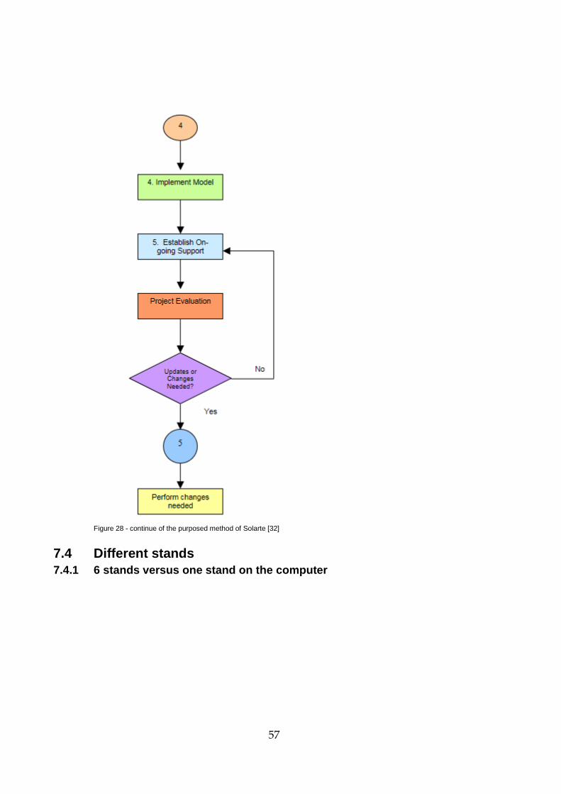
Figure 28 - continue of the purposed method of Solarte [32]
7.4 Different stands
7.4.1 6 stands versus one stand on the computer

58

59

60
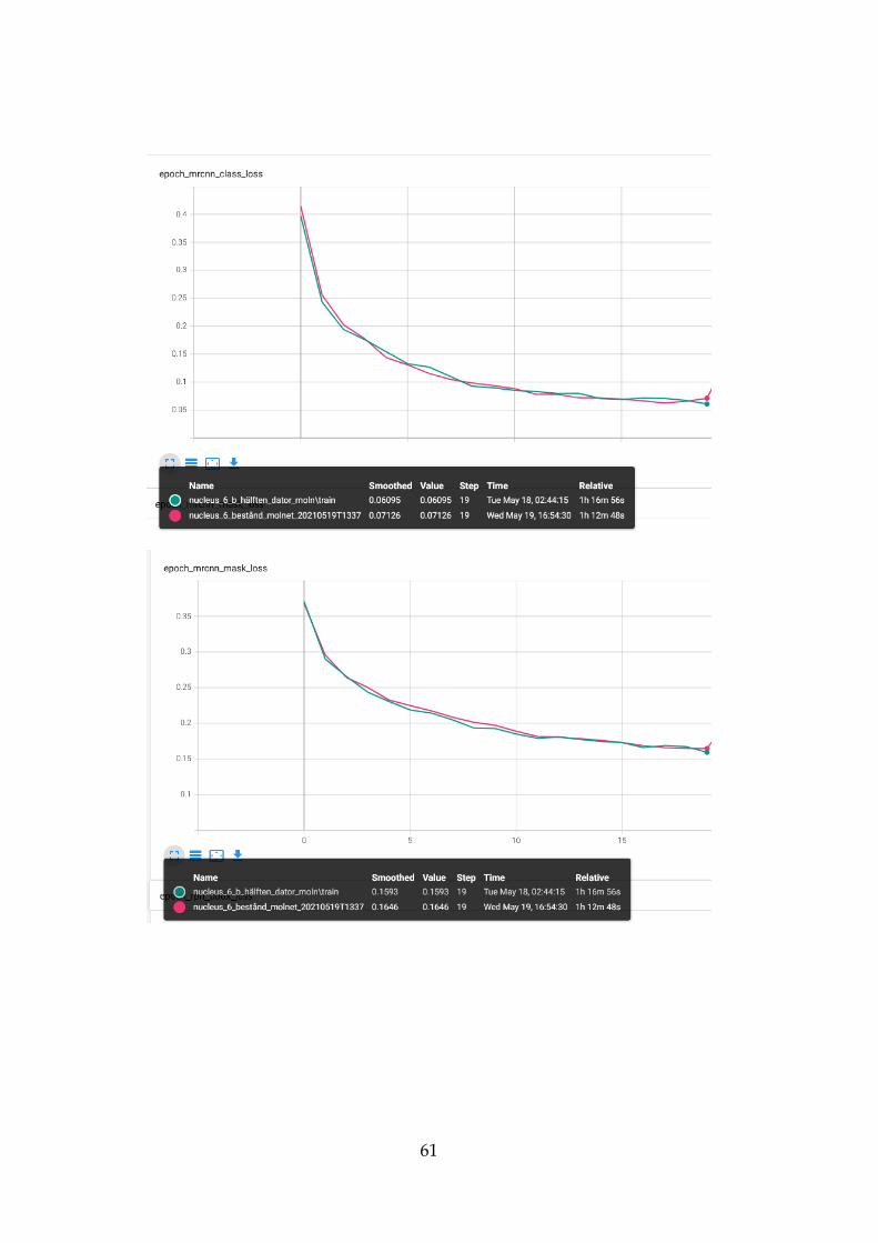
7.4.2 6 stands running on computer versus running it on the cloud
61

62
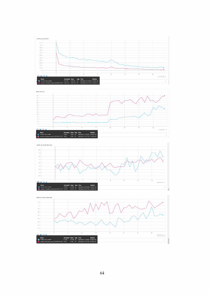
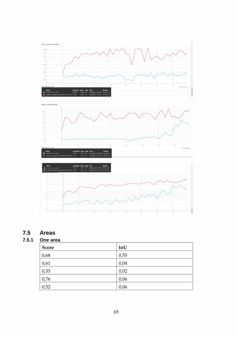
7.4.3 6 stands on the cloud versus 42 stands on the cloud

63
64
65
7.5 Areas
7.5.1 One area
Score IoU
0,68 0,55
0,61 0,04
0,55 0,02
0,76 0,06
0,52 0,06

66
0,73 0,18
0,56 0,06
0,57 0,09
0,63 0,05
0,72 0,00
0,58 0,03
0,61 0,02
0,73 0,46
0,76 0,10
0,72 0,00
0,71 0,03
0,6 0,20
0,8 0,41
0,68 0,44
0,53 0,05
0,77 0,62
0,63 0,00
0,64 0,12
0,77 0,15
0,55 0,14
0,76 0,12
0,52 0,18
0,8 0,01
0,61 0,02
0,6 0,07
0,52 0,14
0,79 0,25
0,57 0,07
0,71 0,05
0,65 0,01
0,72 0,02
0,59 0,09

67
0,6 0,06
0,75 0,23
0,58 0,47
0,51 0,27
0,65 0,3
0,61 0,26
0,54 0,05
0,57 0,07
0,75 0,42
0,57 0,11

68

69
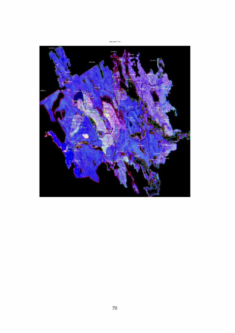
70
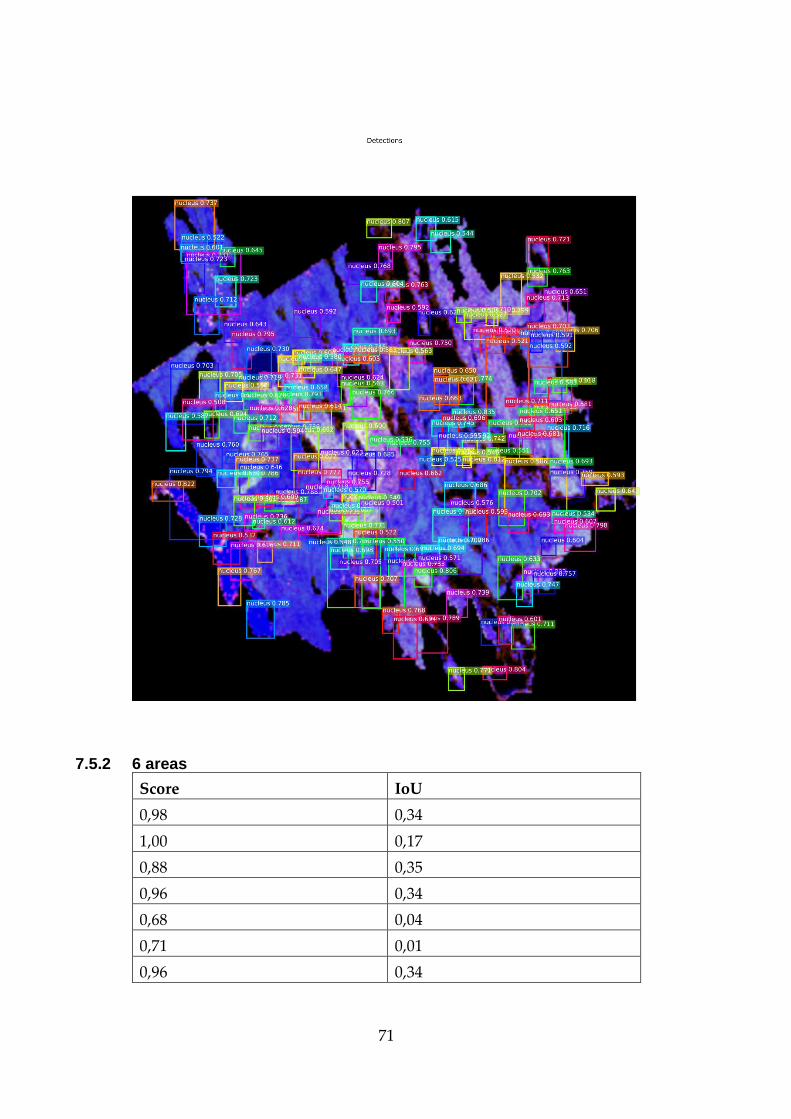
71
7.5.2 6 areas
Score IoU
0,98 0,34
1,00 0,17
0,88 0,35
0,96 0,34
0,68 0,04
0,71 0,01
0,96 0,34

72
0,71 0,32
0,95 0,73
0,91 0,13
0,97 0,41

73
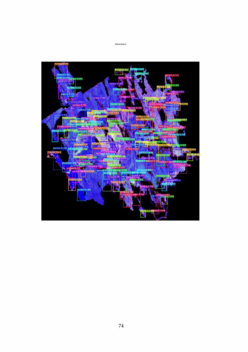
74
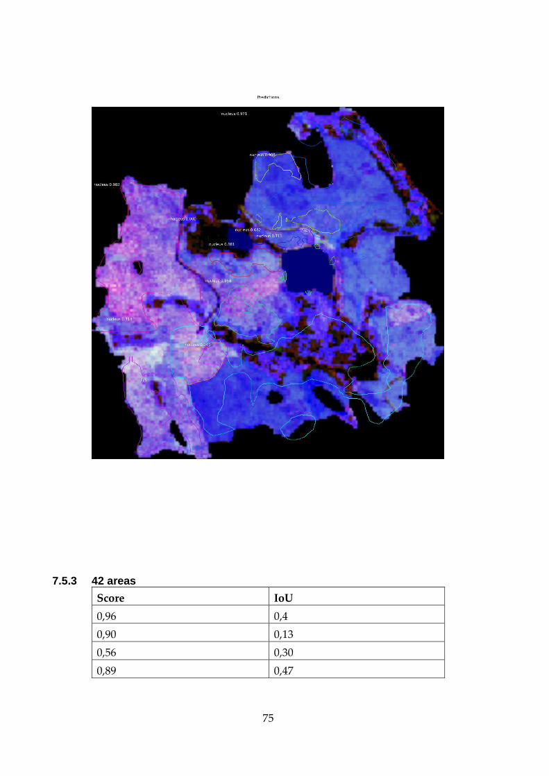
75
7.5.3 42 areas
Score IoU
0,96 0,4
0,90 0,13
0,56 0,30
0,89 0,47
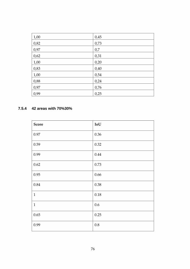
76
1,00 0,45
0,82 0,73
0,97 0,7
0,62 0,31
1,00 0,20
0,83 0,40
1,00 0,54
0,88 0,24
0,97 0,76
0,99 0,25
7.5.4 42 areas with 70%30%
Score IoU
0.97 0.36
0.59 0.32
0.99 0.44
0.62 0.73
0.95 0.66
0.84 0.38
1 0.18
1 0.6
0.65 0.25
0.99 0.8

77
0.96 0.51

78

79

80

81