aiaa 2002-0266 flow control device evaluation for an ...mln/ltrs-pdfs/nasa-aiaa-2002-0266.pdf ·...

AIAA 2002-0266 Flow Control Device Evaluation for an Internal Flow with an Adverse Pressure Gradient L. Jenkins, S. Althoff Gorton, and S. Anders NASA Langley Research Center Hampton, VA

40th AIAA Aerospace Sciences Meeting & Exhibit

14-17 January 2002/Reno, NV

AIAA-2002-0266

American Institute of Aeronautics and Astronautics

1

FLOW CONTROL DEVICE EVALUATION FOR AN INTERNAL FLOW WITH AN ADVERSE PRESSURE GRADIENT

Luther N. Jenkins*, Susan Althoff Gorton†, and Scott G. Anders‡

NASA Langley Research Center Hampton, Virginia

Abstract

The effectiveness of several active and passive devices to control flow in an adverse pressure gradient with secondary flows present was evaluated in the 15 Inch Low Speed Tunnel at NASA Langley Research Center. In this study, passive micro vortex generators, micro bumps, and piezoelectric synthetic jets were evaluated for their flow control characteristics using surface static pressures, flow visualization, and 3D Stereo Digital Particle Image Velocimetry. Data also were acquired for synthetic jet actuators in a zero flow environment. It was found that the micro vortex generator is very effective in controlling the flow environment for an adverse pressure gradient, even in the presence of secondary vortical flow. The mechanism by which the control is effected is a re-energization of the boundary layer through flow mixing. The piezoelectric synthetic jet actuators must have sufficient velocity output to produce strong longitudinal vortices if they are to be effective for flow control. The output of these devices in a laboratory or zero flow environment will be different than the output in a flow environment. In this investigation, the output was higher in the flow environment, but the stroke cycle in the flow did not indicate a positive inflow into the synthetic jet.

Introduction The effect of aviation on the environment and in particular global warming has recently become a focus of study1. In response to environmental concerns and to foster revolutionary propulsion technologies, NASA launched the Ultra Efficient Engine Technology (UEET) program in late 19992. This program has several elements, one of which is to explore the feasibility of the Blended-Wing-Body (BWB) concept as an efficient alternative to conventional transport configurations. The BWB concept has been considered in various forms for several years3-5. Studies have shown that in order to make the largest impact on the vehicle performance, the engines and inlets should be placed near the surface on the _______________________ *Research Engineer, Flow Physics and Control Branch †Research Engineer, Flow Physics and Control Branch, Member AIAA ‡Research Engineer, Flow Physics and Control Branch Copyright 2002 by the American Institute of Aeronautics and Astronautics, Inc. No copyright is asserted in the United States under Title 17, U.S. Code. The U.S. Government has a royalty-free license to exercise all rights under the copyright claimed herein for government purposes. All other rights reserved by the copyright owner.

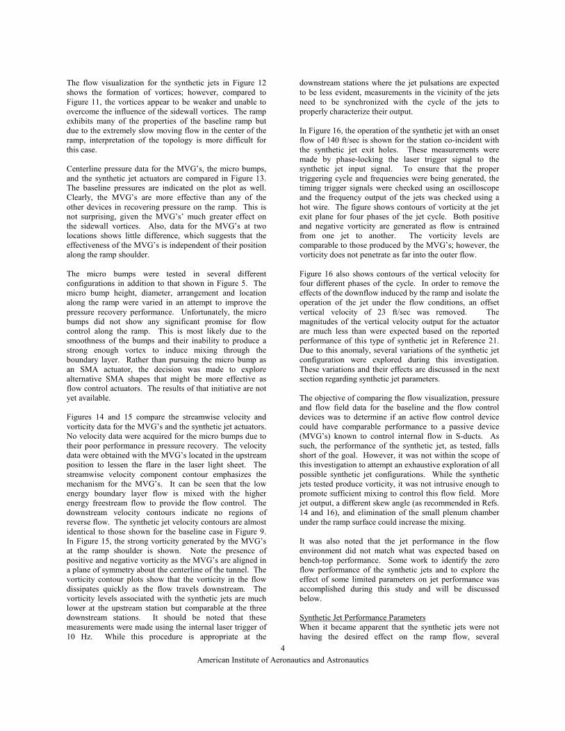
aft section of the vehicle. This configuration of the BWB is shown in Ref. 6 and pictured in Figure 1. When the engines are positioned near the surface, the BWB engine inlet must be an S-duct inlet with the capability to ingest the large boundary layer that will build up over the aircraft body. The inlet must perform this task without producing a significant engine performance penalty in terms of distortion or pressure recovery. Since the boundary layer on the BWB is expected to be on the order of 30% of the inlet height, this presents a challenging task for inlet design. The requirements for inlet performance under the severe conditions of an adverse pressure gradient from the S-duct and a very large onset boundary layer flow have led to the consideration of active flow control devices in the inlet to control the flow. As reported in References 7-25, much research is already underway to identify and develop active flow control devices and technologies and this represents only a sampling of the available material on the subject. There have also been investigations showing the successful use of passive and active flow control technologies applied to inlets. Reference 6 discusses work using passive devices for an S-duct with boundary layer ingestion (BLI), and References 18-20 discuss both passive (microvanes) and active (microjet) concepts applied to aggressive serpentine inlets. The purpose of the present investigation was to lay the groundwork for a future study of active flow control applied to a duct representative of a BWB with BLI. In the present study, the effectiveness of several active and passive devices to control flow in an adverse pressure gradient with secondary flows present was evaluated by examining pressure recovery, flow topology, and flow-field velocity and vorticity characteristics. These data were obtained for passive micro vortex generators, micro bumps, and synthetic jets using surface static pressures, flow visualization, and 3D Stereo Digital Particle Image Velocimetry.

Experimental Apparatus and Methods Facility and Model The experiment was conducted in the NASA Langley 15-Inch Low Speed Tunnel. This tunnel is a closed return, atmospheric facility used primarily for fundamental flow


2

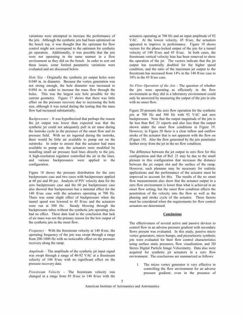
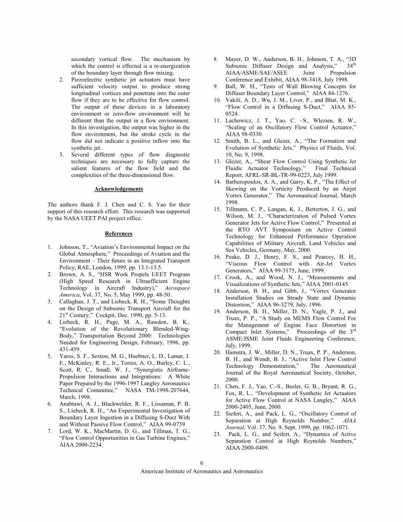
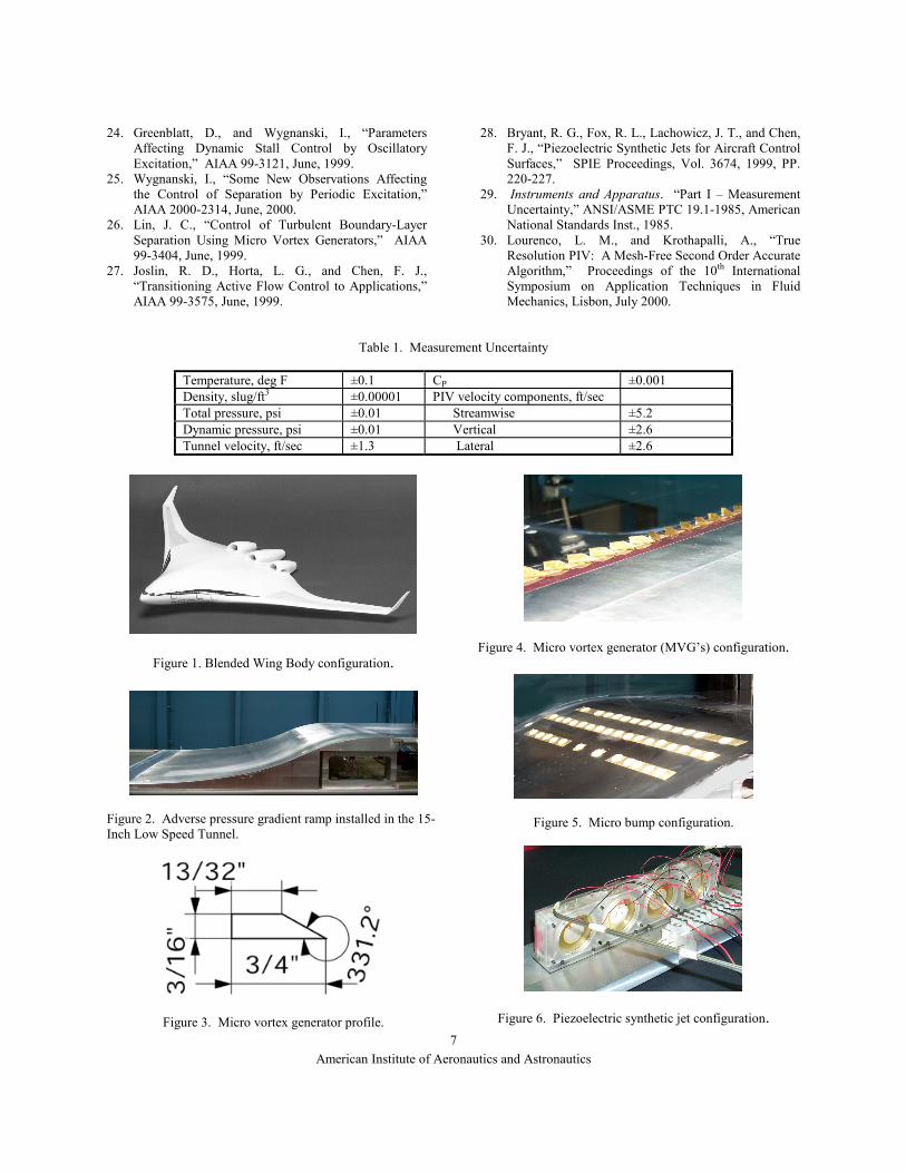
physics research. The maximum flow speed entering the test section is approximately 115 ft/sec. Although the model used for this investigation was not intended to represent any particular inlet shape, it was designed to provide a mildly adverse pressure gradient with separated flow. The model consisted of a long splitter plate installed in the tunnel with an adverse pressure gradient ramp at the aft end. The splitter plate allowed higher flow speeds to be achieved over the test article and provided a flat surface for the upstream boundary layer to develop before being subjected to the adverse pressure gradient. The boundary layer was transitioned by applying grit near the leading edge of the splitter plate and at the corresponding streamwise location on the tunnel walls. The pressure distribution over the splitter plate was adjusted to be uniform between 20 to 50 inches from the leading edge by using supports in the ceiling to slightly modify the ceiling geometry. Flow visualization on the upstream sections of the splitter plate indicated that the flow was two-dimensional except within an inch of the wall boundaries. The adverse pressure gradient ramp section of the model is shown in Figure 2. The ramp geometry was designed to be a Stratford ramp with incipient flow separation at every point along the ramp; however, the adverse pressure gradient created by the ramp caused the sidewall boundary layer to separate and form juncture vortices in the corners of the tunnel. These vorticies, in turn, interacted with the flow over the ramp causing it to separate. The ramp was instrumented with 45 surface static pressure ports located along the centerline and laterally across the ramp at selected model stations. The lateral distribution at each station consisted of five pressure ports equally spaced at 0.5-inch intervals around the centerline of the ramp. Flow Control Devices Numerous flow control devices were considered for their effectiveness in controlling the flow characteristics of the ramp. Several researchers have demonstrated the effectiveness of passive devices such as vortex generators or microvanes for flow improvements in S-ducts and other applications6,10,18-20,26. Microvanes have been shown by experiment and computational effort to be effective in controlling secondary flow and improving pressure recovery and distortion18-20. However, there are indications that active flow control could provide better flow control characteristics and eliminate concerns such as foreign object damage and maintenance issues that hamper the application of micro vortex generators7, 20. In order to provide a baseline passive device for flow control comparisons, micro vortex generators (MVG’s) were used on the shoulder of the ramp. The MVG’s were approximately 20% of the boundary layer height, with a profile as shown in Figure 3. The MVG’s were arranged in a co-rotating pattern at an angle of 23 degrees to the onset flow, and the tunnel centerline provide a plane of symmetry for the configuration as shown in Figure 4. The MVG’s

were installed with the trailing edge at longitudinal (x) station 61.75 for most of the test program. A second passive flow control device tested was a series of micro “bumps.” These bumps were designed to simulate the effect of a shape memory alloy (SMA) actuator on the internal flow of a duct. The bumps were removable plastic pieces in various diameters and heights and were configured in several patterns to evaluate their flow control potential. Figure 5 shows a representative sample of the micro bump configurations installed on the ramp. The only samples available were symmetric in nature and represented a maximum height of approximately 10% of the boundary layer thickness. Four piezo-electric synthetic jets, designed as described in References 21 and 27-28, were incorporated into the model to provide an active flow control mechanism. The synthetic jets were arranged in a lateral series as shown in Figure 6 and installed beneath the ramp shoulder. Each synthetic jet was powered individually through a power amplifier using the same input signal. The synthetic jet output slot was sealed against a small plenum chamber under the ramp surface and the air was able to exit the plenum through a series of eighteen small diameter holes spaced 0.4 inches apart. The holes were located at station 61.75 on the model and angled at 30 degrees up from the surface of the ramp and skewed at 90 degrees to the freestream. The diameter of each hole was originally 0.040 in. but was modified during the test program to be 0.094 in. The original hole spacing and skew angle were designed in early 2000 based on information available at that time. The operating frequency and amplitude of the input signal were established for maximum jet velocity output on the bench before installation using a total pressure probe in a quick-look, optimization procedure. The optimum frequency was found to be 710Hz at an input amplitude of 92 VAC, which was very similar to the optimum reported in Reference 21 for similar actuators. The velocity output was fairly uniform across the eighteen holes. Data Acquisition The flow visualization was obtained using a mixture of kerosene and titanium dioxide to produce a white, paint-like mixture. The mixture was applied to black contact paper mounted on the ramp model. As the tunnel speed was adjusted to the specified test conditions, the local flow transported the paint to various parts of the model. As the kerosene evaporated, the titanium dioxide within the mixture dried on the surface and revealed the surface topology along the ramp. After the paint was dry, the contact paper was marked with fiduciary markings and removed from the surface. The flow-field velocity measurements were made using a 3D Stereo Digital Particle Image Velocimetry (PIV) system. This system consisted of two high resolution video cameras angled at incidence to a laser light sheet that was positioned in a cross-plane to the flow. Due to the


3

incidence of the cameras to the light sheet, all three components of velocity were measured in each PIV measurement plane through stereoscopic vector reconstruction. The light sheet was produced by a pulsed, frequency-doubled, 300mJ Nd:YAG laser operating at 10 Hz. The laser could also be triggered phase-locked to the synthetic jet input signal. In this mode, the laser would fire on multiples of the synthetic jet cycle, as the laser physically could not fire at a faster rate than 10 Hz. At each measurement location, the PIV field of view was approximately 4 inches wide by 3 inches tall, centered along the centerline of the tunnel. The measurement location was carefully aligned with the model system, and the cameras were calibrated with an in-situ target for each location. The tunnel was seeded with atomized mineral oil injected into the flow in the tunnel settling chamber, and the particle size was approximately 5-10 microns. For all conditions, at least thirty samples of PIV data were obtained over a 3 to 6 second period and averaged. The low rms of the mean data indicated that this was enough data to capture the relevant flow features for this investigation. The algorithm used to process the images acquired in this investigation is described in Reference 30. Estimating the accuracy of the stereo PIV measurements is itself a matter of instrumentation research at this time; the best estimate the authors can provide for the accuracy of the PIV velocity measurements is included in Table 1. Test Conditions The main test condition was established by setting the tunnel velocity to 100 ft/sec. This corresponded to a local velocity of 140 ft/sec at station 57 due to the acceleration of the flow above the splitter plate. Station 57 was the farthest aft static surface pressure port location on the flat part of the splitter plate. For this reason, Station 57 conditions are used to define the onset flow to the adverse pressure gradient ramp. The boundary layer was measured at station 57 and found to have a thickness, δ , of approximately 0.87 inches. The boundary profile was converted to wall coordinates and compared with Spalding’s Law. Based on the agreement between the two profiles, the boundary layer was determined to be turbulent.

Discussion of Results Data were obtained for many different configurations and test conditions during this investigation. In this paper, the basic flow over the ramp will be presented to define the baseline flow environment with pressures, flow visualization, and flow field velocity measurements. Comparisons among the different flow control devices will then be presented with respect to the baseline to emphasize the effect of the devices on the flow environment. In the final section, details of several attempts to optimize the synthetic jet output will be given, and the jet performance in a no-flow environment will be presented.

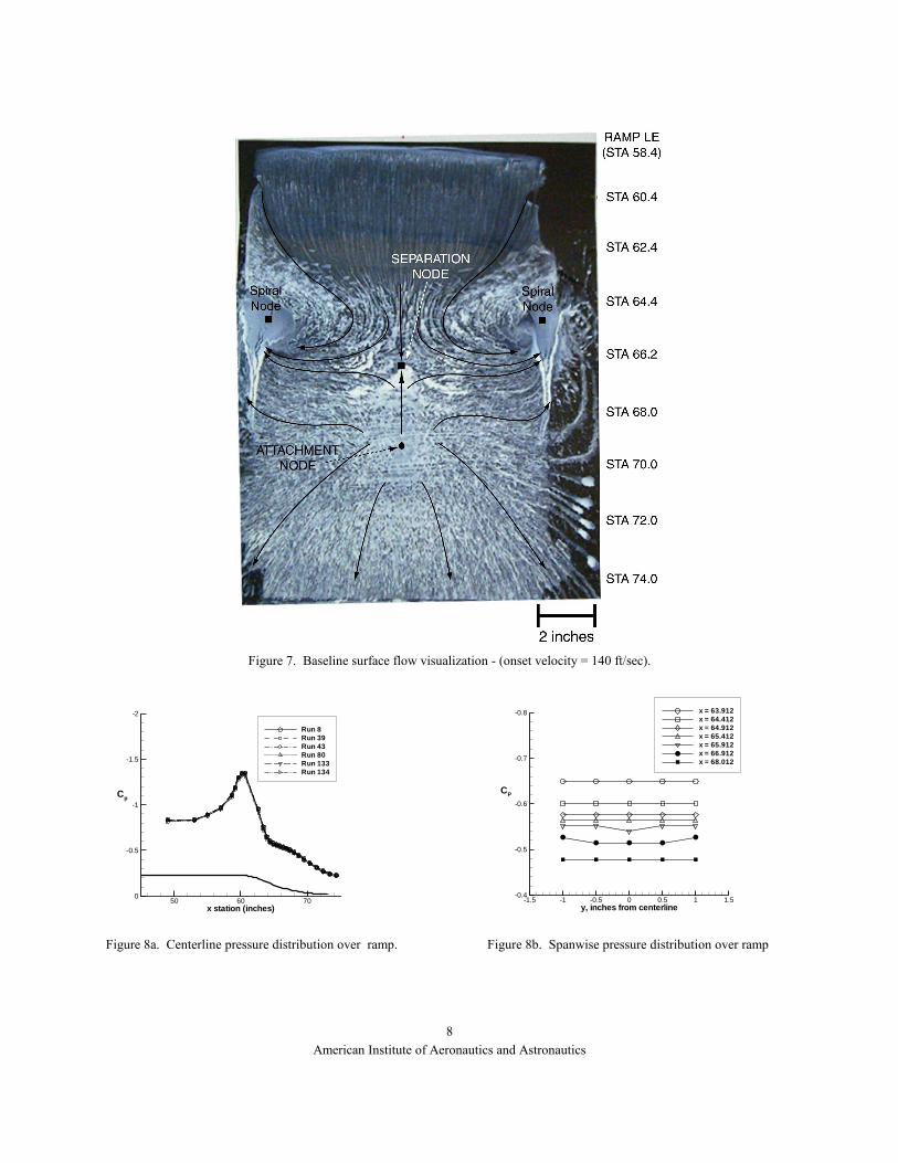
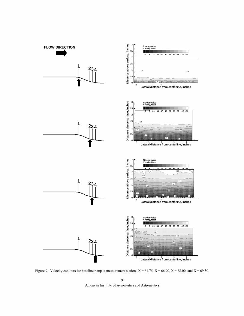
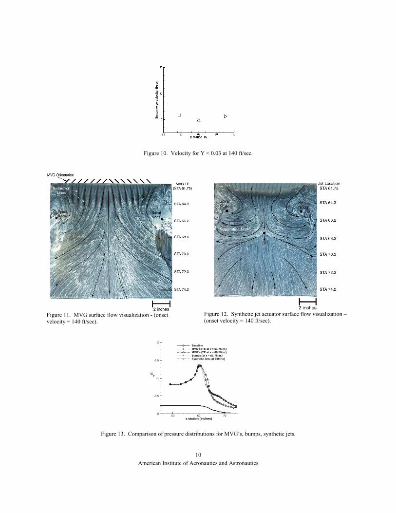
Baseline flow field The baseline configuration flow visualization topology is shown in Figure 7 for the freestream velocity of 140 ft/sec. Although flow along the splitter plate in the tunnel is two-dimensional for the most part, two large spiral nodes reveal the formation of vortical structures. This occurs when the sidewall boundary layer reacts to the adverse pressure gradient near station 61.75 on the ramp. The vortical structures are similar to what might be expected from secondary flow and vortex liftoff in a duct, so no attempt was made to control the vortices for this investigation. Rather, it was thought that the challenges of the strong vortical flow field would provide a better indication of how the flow control devices would work in a realistic inlet configuration. It should be noted that the vortices are highly unsteady and appear to have a trajectory that departs from the surface of the ramp and extends downstream in the tunnel. In addition to the vortical structures, Figure 7 also highlights other significant flow features such as a separation node, an attachment node, and evidence of reverse flow in the center of the ramp. Figure 8 presents the centerline and spanwise surface static pressure distributions for the ramp. In Figure 8a, the repeatability of the baseline pressure profile over a time period of two months and after two major model removals is also shown. The centerline pressure distribution indicates separation occurring near station 64 but does not show the dramatic flow features that the flow visualization revealed. In fact, the spanwise pressure distribution in Fig 8b indicates a fairly uniform and symmetric pressure pattern. In the absence of the other information from the flow visualization and PIV, this type of pressure distribution could easily be interpreted to be representative of uniform, two-dimensional flow. Figure 9 shows velocities measured using PIV along the centerline of the ramp geometry at four longitudinal stations. Each frame consists of at least thirty samples of data acquired at the laser internal trigger frequency of 10 Hz. The contours clearly indicate a thin region of reverse flow in the center of the ramp at station 68.00. The velocity measured very close to the surface on the centerline is plotted in Figure 10 and shows very slow moving and even reversed flow at these locations. Flow Control Devices As described earlier, several flow control devices were applied to the ramp in order to assess their relative ability to control the flow. Figure 11 shows the flow visualization obtained along the ramp for the MVG’s and the synthetic jets. There was no flow visualization obtained for the micro bumps. Note how the MVG’s create a series of strong vortices, as indicated by the dark separation lines, which reduce the influence of the sidewall vortices and allow the flow in the center of the ramp to remain attached.


4

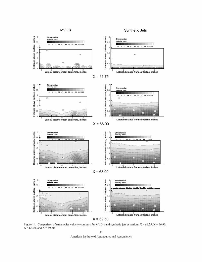
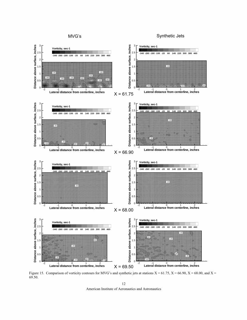
The flow visualization for the synthetic jets in Figure 12 shows the formation of vortices; however, compared to Figure 11, the vortices appear to be weaker and unable to overcome the influence of the sidewall vortices. The ramp exhibits many of the properties of the baseline ramp but due to the extremely slow moving flow in the center of the ramp, interpretation of the topology is more difficult for this case. Centerline pressure data for the MVG’s, the micro bumps, and the synthetic jet actuators are compared in Figure 13. The baseline pressures are indicated on the plot as well. Clearly, the MVG’s are more effective than any of the other devices in recovering pressure on the ramp. This is not surprising, given the MVG’s’ much greater effect on the sidewall vortices. Also, data for the MVG’s at two locations shows little difference, which suggests that the effectiveness of the MVG’s is independent of their position along the ramp shoulder. The micro bumps were tested in several different configurations in addition to that shown in Figure 5. The micro bump height, diameter, arrangement and location along the ramp were varied in an attempt to improve the pressure recovery performance. Unfortunately, the micro bumps did not show any significant promise for flow control along the ramp. This is most likely due to the smoothness of the bumps and their inability to produce a strong enough vortex to induce mixing through the boundary layer. Rather than pursuing the micro bump as an SMA actuator, the decision was made to explore alternative SMA shapes that might be more effective as flow control actuators. The results of that initiative are not yet available. Figures 14 and 15 compare the streamwise velocity and vorticity data for the MVG’s and the synthetic jet actuators. No velocity data were acquired for the micro bumps due to their poor performance in pressure recovery. The velocity data were obtained with the MVG’s located in the upstream position to lessen the flare in the laser light sheet. The streamwise velocity component contour emphasizes the mechanism for the MVG’s. It can be seen that the low energy boundary layer flow is mixed with the higher energy freestream flow to provide the flow control. The downstream velocity contours indicate no regions of reverse flow. The synthetic jet velocity contours are almost identical to those shown for the baseline case in Figure 9. In Figure 15, the strong vorticity generated by the MVG’s at the ramp shoulder is shown. Note the presence of positive and negative vorticity as the MVG’s are aligned in a plane of symmetry about the centerline of the tunnel. The vorticity contour plots show that the vorticity in the flow dissipates quickly as the flow travels downstream. The vorticity levels associated with the synthetic jets are much lower at the upstream station but comparable at the three downstream stations. It should be noted that these measurements were made using the internal laser trigger of 10 Hz. While this procedure is appropriate at the

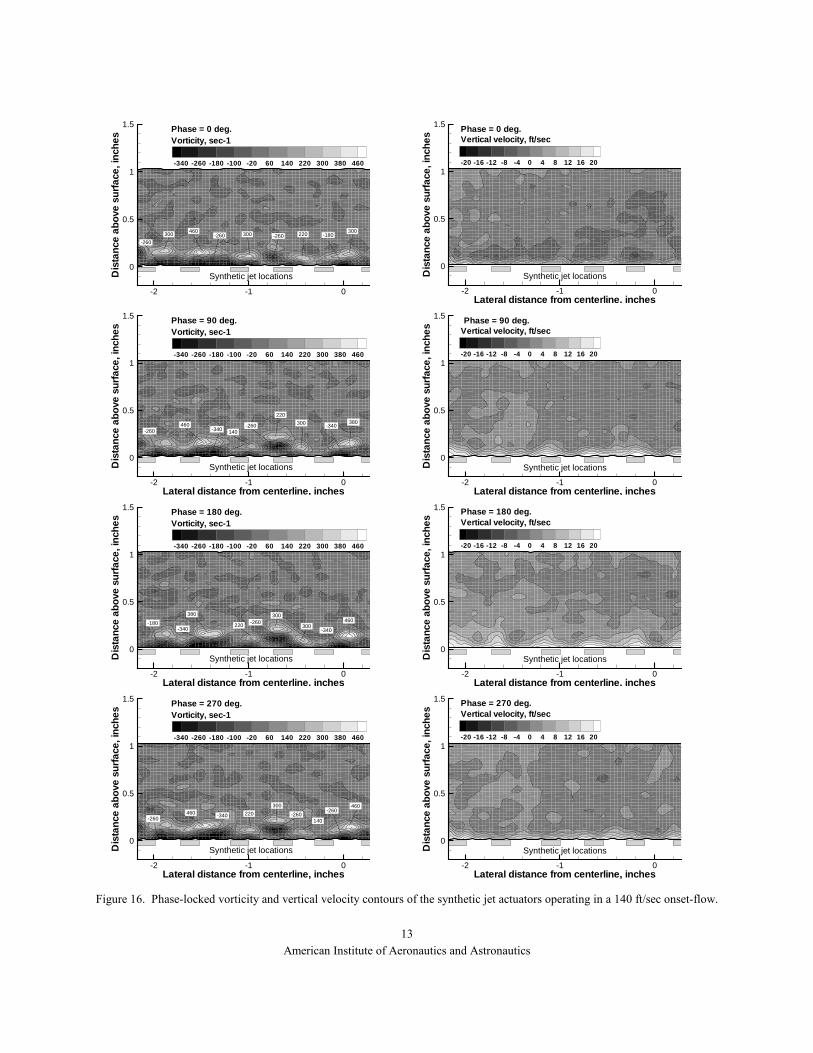
downstream stations where the jet pulsations are expected to be less evident, measurements in the vicinity of the jets need to be synchronized with the cycle of the jets to properly characterize their output. In Figure 16, the operation of the synthetic jet with an onset flow of 140 ft/sec is shown for the station co-incident with the synthetic jet exit holes. These measurements were made by phase-locking the laser trigger signal to the synthetic jet input signal. To ensure that the proper triggering cycle and frequencies were being generated, the timing trigger signals were checked using an oscilloscope and the frequency output of the jets was checked using a hot wire. The figure shows contours of vorticity at the jet exit plane for four phases of the jet cycle. Both positive and negative vorticity are generated as flow is entrained from one jet to another. The vorticity levels are comparable to those produced by the MVG’s; however, the vorticity does not penetrate as far into the outer flow. Figure 16 also shows contours of the vertical velocity for four different phases of the cycle. In order to remove the effects of the downflow induced by the ramp and isolate the operation of the jet under the flow conditions, an offset vertical velocity of 23 ft/sec was removed. The magnitudes of the vertical velocity output for the actuator are much less than were expected based on the reported performance of this type of synthetic jet in Reference 21. Due to this anomaly, several variations of the synthetic jet configuration were explored during this investigation. These variations and their effects are discussed in the next section regarding synthetic jet parameters. The objective of comparing the flow visualization, pressure and flow field data for the baseline and the flow control devices was to determine if an active flow control device could have comparable performance to a passive device (MVG’s) known to control internal flow in S-ducts. As such, the performance of the synthetic jet, as tested, falls short of the goal. However, it was not within the scope of this investigation to attempt an exhaustive exploration of all possible synthetic jet configurations. While the synthetic jets tested produce vorticity, it was not intrusive enough to promote sufficient mixing to control this flow field. More jet output, a different skew angle (as recommended in Refs. 14 and 16), and elimination of the small plenum chamber under the ramp surface could increase the mixing. It was also noted that the jet performance in the flow environment did not match what was expected based on bench-top performance. Some work to identify the zero flow performance of the synthetic jets and to explore the effect of some limited parameters on jet performance was accomplished during this study and will be discussed below. Synthetic Jet Performance Parameters When it became apparent that the synthetic jets were not having the desired effect on the ramp flow, several


5

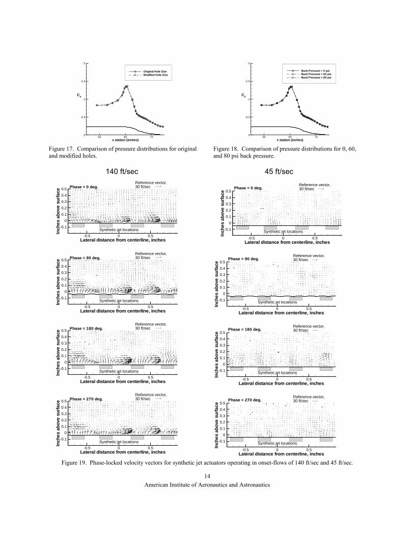
variations were attempted to increase the performance of the jets. Although the synthetic jets had been optimized on the bench top, it was thought that the optimum for flow control might not correspond to the optimum for synthetic jet operation. Additionally, it was possible that the jets were not operating in the same manner in a flow environment as they did on the bench. In order to sort out these issues, some limited parametric variations were evaluated and are discussed below. Hole Size - Originally the synthetic jet output holes were 0.040 in. in diameter. Because the vortex generation was not strong enough, the hole diameter was increased to 0.094 in. in order to increase the mass flow through the holes. This was the largest size hole possible for the current geometry. Figure 17 shows that there was little effect on the pressure recovery due to increasing the hole size, although it was noted during the testing that the mass flow had increased substantially. Backpressure – It was hypothesized that perhaps the reason the jet output was lower than expected was that the synthetic jet could not adequately pull in air mass during the instroke cycle in the presence of the onset flow and its pressure field. With no air ingested during the instroke, there would be little air available to pump out on the outstroke. In order to ensure that the actuator had mass available to pump out, the actuators were modified by installing small air pressure feed lines directly to the jets. A high-resolution regulator controlled the air in the lines, and various backpressures were applied to the configuration. Figure 18 shows the pressure distribution for the zero backpressure case and two cases with backpressure applied at 60 psi and 80 psi. Analysis of PIV velocity data for the zero backpressure case and the 60 psi backpressure case also showed that backpressure has a minimal effect for the 140 ft/sec case with the actuators operating at 700 Hz. There was some slight effect of backpressure when the tunnel speed was lowered to 45 ft/sec and the actuators were run at 300 Hz. Steady blowing through the backpressure tubes without the synthetic jets operating also had no effect. These data lead to the conclusion that lack of air mass was not the primary reason for the low output of the synthetic jets in the onset flow. Frequency – With the freestream velocity at 140 ft/sec, the operating frequency of the jets was swept through a range from 200-1000 Hz with no noticeable effect on the pressure recovery along the ramp. Amplitude – The amplitude of the synthetic jet input signal was swept through a range of 40-92 VAC at a freestream velocity of 140 ft/sec with no significant effect on the pressure recovery data. Freestream Velocity – The freestream velocity was changed in a range from 45 ft/sec to 140 ft/sec with the

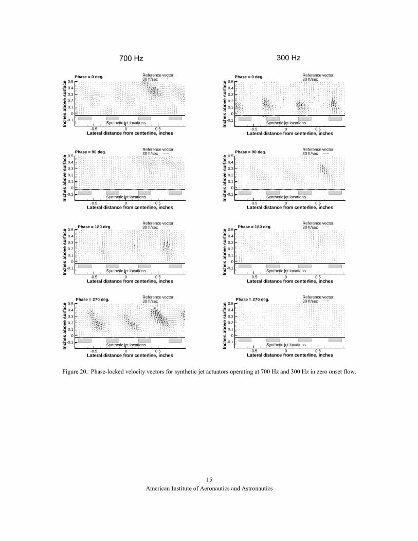
actuators operating at 700 Hz and an input amplitude of 92 VAC. At the lowest velocity, 45 ft/sec, the actuators appeared to improve in performance. Figure 19 shows vectors for the phase-locked output of the jets for a tunnel velocity of 140 ft/sec and 45 ft/sec. In both cases, the freestream vertical velocity bias has been removed to show the operation of the jet. The vectors indicate that the jet output has essentially doubled for the higher speed condition, and the ratio of the maximum jet output to the freestream has increased from 14% in the 140 ft/sec case to 18% in the 45 ft/sec case. No Flow Operation of the Jets - The question of whether the jets were operating as efficiently in the flow environment as they did in a laboratory environment could only be answered by measuring the output of the jets in situ with no onset flow. Figure 20 presents the zero flow operation for the synthetic jets at 700 Hz and 300 Hz with 92 VAC and zero backpressure. Note that the output magnitude of the jets is far less than Ref. 21 reports and also less than the output shown under the onset flow conditions in Figure 19. However, in Figure 20 there is a clear inflow and outflow stroke of the actuator that is not apparent with the flow on (Figure 19). Also the flow generated by the jets penetrates further away from the jet in the no flow condition. The difference between the jet output in zero flow for this configuration and that of Ref. 21 may be due to the small plenum in this configuration that increases the distance between the jet output slot and the surface of the ramp. However, such plenums may be necessary for realistic applications and the performance of the actuator must be improved to account for this. The results of the no onset flow measurements also show that the actuator output in a zero flow environment is lower than what is achieved in an onset flow setting, but the onset flow condition affects the penetration of the velocity into the flow as well as the phasing and stroke cycle of the actuator. These factors must be considered when the requirements for flow control actuators are determined.

Conclusions The effectiveness of several active and passive devices to control flow in an adverse pressure gradient with secondary flows present was evaluated. In this study, passive micro vortex generators, micro bumps, and piezoelectric synthetic jets were evaluated for their flow control characteristics using surface static pressures, flow visualization, and 3D Stereo Digital Particle Image Velocimetry. Data also were acquired for synthetic jet actuators in a zero flow environment. The conclusions are summarized as follows:

1. The micro vortex generator is very effective in controlling the flow environment for an adverse pressure gradient, even in the presence of


6

secondary vortical flow. The mechanism by which the control is effected is a re-energization of the boundary layer through flow mixing.

2. Piezoelectric synthetic jet actuators must have sufficient velocity output to produce strong longitudinal vortices and penetrate into the outer flow if they are to be effective for flow control. The output of these devices in a laboratory environment or zero-flow environment will be different than the output in a flow environment. In this investigation, the output was higher in the flow environment, but the stroke cycle in the flow did not indicate a positive inflow into the synthetic jet.

3. Several different types of flow diagnostic techniques are necessary to fully capture the salient features of the flow field and the complexities of the three-dimensional flow.

Acknowledgements

The authors thank F. J. Chen and C. S. Yao for their support of this research effort. This research was supported by the NASA UEET PAI project office.

References 1. Johnson, T., “Aviation’s Environmental Impact on the

Global Atmosphere,” Proceedings of Aviation and the Environment – Their future in an Integrated Transport Policy, RAE, London, 1999, pp. 13.1-13.5.

2. Brown, A. S., “HSR Work Propels UEET Program (High Speed Research in Ultraefficient Engine Technology in Aircraft Industry),” Aerospace America, Vol. 37, No. 5, May 1999, pp. 48-50.

3. Callaghan, J. T., and Liebeck, R. H., “Some Thoughts on the Design of Subsonic Transport Aircraft for the 21st Century,” Cockpit, Dec. 1990, pp. 5-13.

4. Liebeck, R. H., Page, M. A., Rawdon, B. K., “Evolution of the Revolutionary Blended-Wing-Body,” Transportation Beyond 2000: Technologies Needed for Engineering Design, February, 1996, pp. 431-459.

5. Yaros, S. F., Sexton, M. G., Huebner, L. D., Lamar, J. E., McKinley, R. E., Jr., Torres, A. O., Burley, C. L., Scott, R. C., Small, W. J., “Synergistic Airframe-Propulsion Interactions and Integrations: A White Paper Prepared by the 1996-1997 Langley Aeronautics Technical Committee,” NASA TM-1998-207644, March, 1998.

6. Anabtawi, A. J., Blackwelder, R. F., Lissaman, P. B. S., Liebeck, R. H., “An Experimental Investigation of Boundary Layer Ingestion in a Diffusing S-Duct With and Without Passive Flow Control,” AIAA 99-0739

7. Lord, W. K., MacMartin, D. G., and Tillman, T. G., “Flow Control Opportunities in Gas Turbine Engines,” AIAA 2000-2234.

8. Mayer, D. W., Anderson, B. H., Johnson, T. A., “3D Subsonic Diffuser Design and Analysis,” 34th AIAA/ASME/SAE/ASEE Joint Propulsion Conference and Exhibit, AIAA 98-3418, July 1998.

9. Ball, W. H., “Tests of Wall Blowing Concepts for Diffuser Boundary Layer Control,” AIAA 84-1276.

10. Vakili, A. D., Wu, J. M., Liver, P., and Bhat, M. K., “Flow Control in a Diffusing S-Duct,” AIAA 85-0524.

11. Lachowicz, J. T., Yao, C. –S., Wlezien, R. W., “Scaling of an Oscillatory Flow Control Actuator,” AIAA 98-0330.

12. Smith, B. L., and Glezer, A., “The Formation and Evolution of Synthetic Jets,” Physics of Fluids, Vol. 10, No. 9, 1998.

13. Glezer, A., “Shear Flow Control Using Synthetic Jet Fluidic Actuator Technology,” Final Technical Report, AFRL-SR-BL-TR-99-0223, July 1999.

14. Barberopoulos, A. A., and Garry, K. P., “The Effect of Skewing on the Vorticity Produced by an Airjet Vortex Generator,” The Aeronautical Journal, March 1998.

15. Tillmann, C. P., Langan, K. J., Betterton, J. G., and Wilson, M. J., “Characterization of Pulsed Vortex Generator Jets for Active Flow Control,” Presented at the RTO AVT Symposium on Active Control Technology for Enhanced Performance Operation Capabilities of Military Aircraft, Land Vehicles and Sea Vehicles, Germany, May, 2000.

16. Peake, D. J., Henry, F. S., and Pearcey, H. H., “Viscous Flow Control with Air-Jet Vortex Generators,” AIAA 99-3175, June, 1999.

17. Crook, A., and Wood, N. J., “Measurements and Visualizations of Synthetic Jets,” AIAA 2001-0145.

18. Anderson, B. H., and Gibb, J., “Vortex Generator Installation Studies on Steady State and Dynamic Distortion,” AIAA 96-3279, July, 1996.

19. Anderson, B. H., Miller, D. N., Yagle, P. J., and Truax, P. P., “A Study on MEMS Flow Control For the Management of Engine Face Distortion in Compact Inlet Systems,” Proceedings of the 3rd ASME/JSME Joint Fluids Engineering Conference, July, 1999.

20. Hamstra, J. W., Miller, D. N., Truax, P. P., Anderson, B. H., and Wendt, B. J., “Active Inlet Flow Control Technology Demonstration,” The Aeronautical Journal of the Royal Aeronautical Society, October, 2000.

21. Chen, F. J., Yao, C.-S., Beeler, G. B., Bryant, R. G., Fox, R. L., “Development of Synthetic Jet Actuators for Active Flow Control at NASA Langley,” AIAA 2000-2405, June, 2000.

22. Siefert, A., and Pack, L. G., “Oscillatory Control of Separation at High Reynolds Number,” AIAA Journal, Vol. 37, No. 9, Sept. 1999, pp. 1062-1071.

23. Pack, L. G., and Seifert, A., “Dynamics of Active Separation Control at High Reynolds Numbers,” AIAA 2000-0409.


7

24. Greenblatt, D., and Wygnanski, I., “Parameters Affecting Dynamic Stall Control by Oscillatory Excitation,” AIAA 99-3121, June, 1999.

25. Wygnanski, I., “Some New Observations Affecting the Control of Separation by Periodic Excitation,” AIAA 2000-2314, June, 2000.

26. Lin, J. C., “Control of Turbulent Boundary-Layer Separation Using Micro Vortex Generators,” AIAA 99-3404, June, 1999.

27. Joslin, R. D., Horta, L. G., and Chen, F. J., “Transitioning Active Flow Control to Applications,” AIAA 99-3575, June, 1999.

28. Bryant, R. G., Fox, R. L., Lachowicz, J. T., and Chen, F. J., “Piezoelectric Synthetic Jets for Aircraft Control Surfaces,” SPIE Proceedings, Vol. 3674, 1999, PP. 220-227.

29. Instruments and Apparatus. “Part I – Measurement Uncertainty,” ANSI/ASME PTC 19.1-1985, American National Standards Inst., 1985.

30. Lourenco, L. M., and Krothapalli, A., “True Resolution PIV: A Mesh-Free Second Order Accurate Algorithm,” Proceedings of the 10th International Symposium on Application Techniques in Fluid Mechanics, Lisbon, July 2000.

Table 1. Measurement Uncertainty

Temperature, deg F ±0.1 CP ±0.001 Density, slug/ft3 ±0.00001 PIV velocity components, ft/sec Total pressure, psi ±0.01 Streamwise ±5.2 Dynamic pressure, psi ±0.01 Vertical ±2.6 Tunnel velocity, ft/sec ±1.3 Lateral ±2.6

Figure 1. Blended Wing Body configuration.

Figure 2. Adverse pressure gradient ramp installed in the 15-Inch Low Speed Tunnel.

Figure 3. Micro vortex generator profile.

Figure 4. Micro vortex generator (MVG’s) configuration.

Figure 5. Micro bump configuration.

Figure 6. Piezoelectric synthetic jet configuration.


8

Figure 7. Baseline surface flow visualization - (onset velocity = 140 ft/sec).

x station (inches)50 60 70

-2

-1.5

-1

-0.5

0

Run 8Run 39Run 43Run 80Run 133Run 134

Cp

Figure 8a. Centerline pressure distribution over ramp.

y, inches from centerline-1.5 -1 -0.5 0 0.5 1 1.5

-0.8

-0.7

-0.6

-0.5

-0.4

x = 63.912x = 64.412x = 64.912x = 65.412x = 65.912x = 66.912x = 68.012

CP

Figure 8b. Spanwise pressure distribution over ramp


9

2134

125

1259986

125

Lateral distance from centerline, inches

Dis

tan

ceab

ove

surf

ace,

inch

es

-2 -1 0 1 20

0.5

1

1.5

2

2.5

3

-5 8 21 34 47 60 73 86 99 112 125

Velocity, ft/secStreamwise

2134

125

99

47

218 8

86


Dis

tan

ceab

ove

surf

ace,

inch

es

-2 -1 0 1 20

0.5

1

1.5

2

2.5

3

-5 8 21 34 47 60 73 86 99 112 125


2134

112

125

73

47

-5

112

86

218

8-5-5-58


Dis

tan

ceab

ove

surf

ace,

inch

es

-2 -1 0 1 20

0.5

1

1.5

2

2.5

3

-5 8 21 34 47 60 73 86 99 112 125


2134

112

86

60

47

21

112

8

99


Dis

tan

ceab

ove

surf

ace,

inch

es

-2 -1 0 1 20

0.5

1

1.5

2

2.5

3

-5 8 21 34 47 60 73 86 99 112 125

Velocity, ft/secStreamwiseVelocity, ft/sec

Figure 9. Velocity contours for baseline ramp at measurement stations X = 61.75, X = 66.90, X = 68.00, and X = 69.50.

FLOW DIRECTION


10

Figure 10. Velocity for Y < 0.03 at 140 ft/sec.

Figure 11. MVG surface flow visualization - (onset velocity = 140 ft/sec).

Figure 12. Synthetic jet actuator surface flow visualization – (onset velocity = 140 ft/sec).


-2

-1.5

-1

-0.5

0

BaselineMVG’s (TE at x = 61.75 in.)MVG’s (TE at x = 60.50 in.)Bumps (at x = 61.75 in.)Synthetic Jets (at 700 Hz)

Cp

Figure 13. Comparison of pressure distributions for MVG’s, bumps, synthetic jets.


11

125

125

125

99 86

8699


Dis

tanc

eab

ove

surf

ace,

inch

es

-2 -1 0 1 20

0.5

1

1.5

2

2.5

3

-5 8 21 34 47 60 73 86 99 112 125


125

86

125112


Dis

tan

ceab

ove

surf

ace,

inch

es

-2 -1 0 1 20

0.5

1

1.5

2

2.5

3

-5 8 21 34 47 60 73 86 99 112 125

StreamwiseVelocity, ft/sec

125

125

125

8686

8699


Dis

tan

ceab

ove

surf

ace,

inch

es

-2 -1 0 1 20

0.5

1

1.5

2

2.5

3

-5 8 21 34 47 60 73 86 99 112 125


125

125

73

21

47

34

73

8


Dis

tan

ceab

ove

surf

ace,

inch

es

-2 -1 0 1 20

0.5

1

1.5

2

2.5

3

-5 8 21 34 47 60 73 86 99 112 125


125

125

112

99

47 47

60

73

73

34


Dis

tan

ceab

ove

surf

ace,

inch

es

-2 -1 0 1 20

0.5

1

1.5

2

2.5

3

-5 8 21 34 47 60 73 86 99 112 125


125

125

112

60

8

47

21

60

8


Dis

tan

ceab

ove

surf

ace,

inch

es

-2 -1 0 1 20

0.5

1

1.5

2

2.5

3

-5 8 21 34 47 60 73 86 99 112 125


112

112

112

73 6086

86

73

99

60


Dis

tan

ceab

ove

surf

ace,

inch

es

-2 -1 0 1 20

0.5

1

1.5

2

2.5

3

-5 8 21 34 47 60 73 86 99 112 125

Velocity, ft/secStreamwiseVelocity, ft/secVelocity, ft/secVelocity, ft/sec

112

125

99

47

8

34

21

47

8


Dis

tan

ceab

ove

surf

ace,

inch

es

-2 -1 0 1 20

0.5

1

1.5

2

2.5

3

-5 8 21 34 47 60 73 86 99 112 125


Figure 14. Comparison of streamwise velocity contours for MVG’s and synthetic jets at stations X = 61.75, X = 66.90, X = 68.00, and X = 69.50.

X = 66.90

X = 61.75

X = 68.00

X = 69.50

MVG’s Synthetic Jets


12


Dis

tan

ceab

ove

surf

ace,

inch

es

-2 -1 0 1 20

0.5

1

1.5

2

2.5

3

-340 -260 -180 -100 -20 60 140 220 300 380 460

Vorticity, sec-1

-340 -100

-100

140

220

460300

-180

-340

-20

140 220 60


Dis

tan

ceab

ove

surf

ace,

inch

es

-2 -1 0 1 20

0.5

1

1.5

2

2.5

3

-340 -260 -180 -100 -20 60 140 220 300 380 460

Vorticity, sec-1

-20

-2060

6060-100


Dis

tan

ceab

ove

surf

ace,

inch

es

-2 -1 0 1 20

0.5

1

1.5

2

2.5

3

-340 -260 -180 -100 -20 60 140 220 300 380 460

Vorticity, sec-1

-20

-20


Dis

tan

ceab

ove

surf

ace,

inch

es

-2 -1 0 1 20

0.5

1

1.5

2

2.5

3

-340 -260 -180 -100 -20 60 140 220 300 380 460

Vorticity, sec-1

-20


Dis

tan

ceab

ove

surf

ace,

inch

es

-2 -1 0 1 20

0.5

1

1.5

2

2.5

3

-340 -260 -180 -100 -20 60 140 220 300 380 460

Vorticity, sec-1

-20


Dis

tan

ceab

ove

surf

ace,

inch

es

-2 -1 0 1 20

0.5

1

1.5

2

2.5

3

-340 -260 -180 -100 -20 60 140 220 300 380 460

Vorticity, sec-1

-20

-2060

0-20

60


Dis

tan

ceab

ove

surf

ace,

inch

es

-2 -1 0 1 20

0.5

1

1.5

2

2.5

3

-340 -260 -180 -100 -20 60 140 220 300 380 460

Vorticity, sec-1

140

60

-20

-20

60-20


Dis

tan

ceab

ove

surf

ace,

inch

es

-2 -1 0 1 20

0.5

1

1.5

2

2.5

3

-340 -260 -180 -100 -20 60 140 220 300 380 460

Vorticity, sec-1

Figure 15. Comparison of vorticity contours for MVG’s and synthetic jets at stations X = 61.75, X = 66.90, X = 68.00, and X = 69.50.

X = 69.50

X = 61.75

X = 68.00

X = 66.90

MVG’s Synthetic Jets


13

Dis

tan

ceab

ove

surf

ace,

inch

es

-2 -1 0

0

0.5

1

1.5

-340 -260 -180 -100 -20 60 140 220 300 380 460

Vorticity, sec-1Phase = 0 deg.

Synthetic jet locations

-260

300-180220-260300-260

460300


Dis

tanc

eab

ove

surf

ace,

inch

es

-2 -1 0

0

0.5

1

1.5

-20 -16 -12 -8 -4 0 4 8 12 16 20

Vertical velocity, ft/sec


Phase = 0 deg.


Dis

tanc

eab

ove

surf

ace,

inch

es

-2 -1 0

0

0.5

1

1.5

-340 -260 -180 -100 -20 60 140 220 300 380 460



-340380380

-260

300

220

380-260140-340

460


Dis

tanc

eab

ove

surf

ace,

inch

es

-2 -1 0

0

0.5

1

1.5

-20 -16 -12 -8 -4 0 4 8 12 16 20



Phase = 90 deg.


Dis

tanc

eab

ove

surf

ace,

inch

es

-2 -1 0

0

0.5

1

1.5

-340 -260 -180 -100 -20 60 140 220 300 380 460



460-180

380

-340220

-260300

300-340


Dis

tanc

eab

ove

surf

ace,

inch

es

-2 -1 0

0

0.5

1

1.5

-20 -16 -12 -8 -4 0 4 8 12 16 20

Vertical velocity, ft/secPhase = 180 deg.



Dis

tanc

eab

ove

surf

ace,

inch

es

-2 -1 0

0

0.5

1

1.5

-340 -260 -180 -100 -20 60 140 220 300 380 460



460

-260-260-340460 220

300

-260140

-260


Dis

tanc

eab

ove

surf

ace,

inch

es

-2 -1 0

0

0.5

1

1.5

-20 -16 -12 -8 -4 0 4 8 12 16 20



Phase = 270 deg.

Figure 16. Phase-locked vorticity and vertical velocity contours of the synthetic jet actuators operating in a 140 ft/sec onset-flow.


14


-2

-1.5

-1

-0.5

0

Original Hole SizeModified Hole Size

Cp

Figure 17. Comparison of pressure distributions for original and modified holes.


-2

-1.5

-1

-0.5

0

Back Pressure = 0 psiBack Pressure = 60 psiBack Pressure = 80 psi

Cp

Figure 18. Comparison of pressure distributions for 0, 60, and 80 psi back pressure.


Inch

esab

ove

surf

ace

-0.5 0 0.5

-0.1

0

0.1

0.2

0.3

0.4

0.5


Phase = 0 deg.Reference vector,30 ft/sec


Inch

esab

ove

surf

ace

-0.5 0 0.5

-0.1

0

0.1

0.2

0.3

0.4

0.5




Inch

esab

ove

surf

ace

-0.5 0 0.5

-0.1

0

0.1

0.2

0.3

0.4

0.5




Inch

esab

ove

surf

ace

-0.5 0 0.5

-0.1

0

0.1

0.2

0.3

0.4

0.5




Inch

esab

ove

surf

ace

-0.5 0 0.5

-0.1

0

0.1

0.2

0.3

0.4

0.5 Phase = 180 deg.


Reference vector,30 ft/sec


Inch

esab

ove

surf

ace

-0.5 0 0.5

-0.1

0

0.1

0.2

0.3

0.4

0.5Phase = 180 deg.




Inch

esab

ove

surf

ace

-0.5 0 0.5

-0.1

0

0.1

0.2

0.3

0.4

0.5




Inch

esab

ove

surf

ace

-0.5 0 0.5

-0.1

0

0.1

0.2

0.3

0.4

0.5



Figure 19. Phase-locked velocity vectors for synthetic jet actuators operating in onset-flows of 140 ft/sec and 45 ft/sec.

140 ft/sec 45 ft/sec


15


Inch

esab

ove

surf

ace

-0.5 0 0.5

-0.1

0

0.1

0.2

0.3

0.4

0.5


Phase = 0 deg. Reference vector,30 ft/sec


Inch

esab

ove

surf

ace

-0.5 0 0.5

-0.1

0

0.1

0.2

0.3

0.4

0.5




Inch

esab

ove

surf

ace

-0.5 0 0.5

-0.1

0

0.1

0.2

0.3

0.4

0.5




Inch

esab

ove

surf

ace

-0.5 0 0.5

-0.1

0

0.1

0.2

0.3

0.4

0.5




Inch

esab

ove

surf

ace

-0.5 0 0.5

-0.1

0

0.1

0.2

0.3

0.4

0.5Phase = 180 deg.




Inch

esab

ove

surf

ace

-0.5 0 0.5

-0.1

0

0.1

0.2

0.3

0.4

0.5Phase = 180 deg.




Inch

esab

ove

surf

ace

-0.5 0 0.5

-0.1

0

0.1

0.2

0.3

0.4

0.5




Inch

esab

ove

surf

ace

-0.5 0 0.5

-0.1

0

0.1

0.2

0.3

0.4

0.5



Figure 20. Phase-locked velocity vectors for synthetic jet actuators operating at 700 Hz and 300 Hz in zero onset flow.

700 Hz 300 Hz

aiaa 2002-0266 flow control device evaluation for an ...mln/ltrs-pdfs/nasa-aiaa-2002-0266.pdf ·...

Documents