aiaa-2013-2567-charest

A High-Order Central ENO Finite-Volume Scheme forThree-Dimensional Turbulent Reactive Flows on Unstructured

Mesh

M. R.J. Charest∗ and C. P.T. Groth†

University of Toronto Institute for Aerospace Studies

4925 Dufferin Street, Toronto, Ontario, Canada, M3H 5T6

High-order discretization techniques offer the potential to significantly reduce the computational costs nec-essary to obtain accurate predictions when compared to lower-order methods. However, efficient, universally-applicable, high-order discretizations remain somewhat illusive, especially for more arbitrary unstructuredmeshes and for large-eddy simulation (LES) of turbulent reacting flows. A novel, high-order, central essentiallynon-oscillatory (CENO), cell-centered, finite-volume scheme is proposed for the solution of the conservationequations of turbulent, reactive, low speed flows on three-dimensional unstructured meshes. The proposedscheme is applied to the pseudo-compressibility formulation of the Favre-filtered governing equations andthe resulting discretized equations are solved with a parallel implicit Newton-Krylov algorithm. Temporalderivatives are discretized using the family of high-order backward difference formulas (BDF) and the re-sulting equations are solved via a dual-time stepping approach. Large-eddy simulations of a laboratory-scaleturbulent flame is carried out and the proposed finite-volume scheme is validated against experimental mea-surements. The high-order scheme is demonstrated to provide both reliable and accurate solutions for complexturbulent reactive flows.

I. Introduction

Many practical flows that are relevant to science and engineering present significant challenges to model numeri-cally, primarily due to the wide range of scales and physical/chemical phenomena involved. Such flows include, butare not limited to, multiphase, turbulent, and combusting flows encountered in propulsion systems (e.g., gas turbineengines and solid propellant rocket motors). Nonetheless, computational fluid dynamics (CFD) has proven to be animportant enabling technology in these areas. But for most of these practical flows, there is currently a limit on whatcan be simulated because of the complexities in the physics and the range of scales that must be resolved. For exam-ple, direct numerical simulation (DNS) of full-scale practical turbulent flows is not possible. Therefore, mathematicalmodels of these complex flows must rely heavily on engineering approximations and sophisticated numerical methodsto represent the underlying physics and ensure that computations remain tractable.

The primary approaches for modelling turbulent flows are Reynolds-Averaged Navier-Stokes (RANS) and Large-Eddy Simulation (LES)1,2. RANS-based methods are more commonly used in engineering applications due to theircomputational efficiency. However, they cannot resolve any part of the turbulent fluctuations since information re-garding fluctuations is lost through the averaging process. LES separates the turbulent scales via a low-pass filteringprocess applied to the governing equations and, as a result, provides information about the large-scale turbulent fluc-tuations. As such, LES is considered an intermediate between DNS and RANS since LES resolves the large-scalemotions of the flow and models the small scales.

Despite the physical simplifications employed by LES, LES of full-scale practical turbulent reactive flows stillrequires significant computational resources. One promising numerical technique to reduce the computational costassociated with LES calculations is the use of high-order methods (i.e., methods higher than second order). High-order methods are more accurate than standard low-order methods (i.e, methods up to second order) and also offerimproved numerical efficiency since fewer computational cells are required to achieve a desired level of accuracy3.∗Post-Doctoral Fellow, UTIAS, [email protected], Member AIAA.†Professor, UTIAS, [email protected], Senior Member AIAA.

1 of 21

American Institute of Aeronautics and Astronautics

Dow

nloa

ded

by C

linto

n G

roth

on

July

11,

201

3 | h

ttp://

arc.

aiaa

.org

| D

OI:

10.

2514

/6.2

013-

2567

21st AIAA Computational Fluid Dynamics Conference

June 24-27, 2013, San Diego, CA

AIAA 2013-2567

Copyright © 2013 by the American Institute of Aeronautics and Astronautics, Inc. All rights reserved.

However, these advantages of high-order methods are difficult to fully realize because of the conflicting relation-ship between accuracy and robustness. For hyperbolic conservation laws and/or compressible flow simulations, themain challenge involves obtaining accurate discretizations while ensuring that discontinuities and shocks are handledreliably and robustly4. High-order schemes for elliptic partial differential equations (PDEs) should satisfy a maxi-mum principle while remaining accurate5. Additionally, modelling reacting flows requires integrating numericallystiff and mathematically complex source terms over the computational domain. There are many studies of high-orderschemes developed for finite-volume4,6–15, discontinuous Galerkin16–20, and spectral finite-difference/finite-volumemethods21–25 on both structured and unstructured mesh. In spite of many advances, there is still no consensus for a ro-bust, efficient, and accurate scheme that fully deals with all of the aforementioned issues and is universally applicableto arbitrary meshes.

Ivan and Groth 26,27 proposed a high-order Central Essentially Non Oscillatory (CENO), cell-centered, finite-volume scheme that was demonstrated to remain both accurate and robust in a variety of physically-complex flows.The CENO scheme uses a fixed central stencil which avoids the difficulties encountered by standard and weightedENO schemes4,10,12,13 that result from the use of variable stencils. With ENO and WENO schemes, selecting theappropriate stencils on general multi-dimensional unstructured meshes is not straightforward7,8,11,28 and using thesestencils can produce poor conditioning of the linear systems involved in performing the solution reconstruction11,28.

The CENO scheme is based on a hybrid solution reconstruction procedure that combines an unlimited high-orderk-exact, least-squares reconstruction technique with a monotonicity preserving limited piecewise linear least-squaresreconstruction algorithm. Fixed central stencils are used for both the unlimited high-order k-exact reconstruction andthe limited piecewise linear reconstruction. Switching between the two reconstruction algorithms is determined bya solution smoothness indicator that indicates whether or not the solution is resolved on the computational mesh.Originally developed for structured two-dimensional mesh, this scheme has been successfully extended to two- andthree-dimensional unstructured mesh and applied to a variety of inviscid and viscous flows by McDonald et al. 29 ,Charest et al. 30 .

In the present research, the high-order CENO finite-volume scheme is extended to solve the equations governinglow-Mach-number, turbulent, reactive flows on unstructured mesh. The ability of the scheme to accurately modelturbulent flames is demonstrated using a LES approach coupled with an eddy-dissipation-based model for turbulence-chemistry interactions. The resulting governing equations are solved using the pseudo-compressibility approach cou-pled with an implicit Newton-Krylov algorithm. The algorithm is applied to a laboratory scale turbulent premixedflame and analyzed in terms of accuracy and robustness. In particular, low- and high-order numerical predictions arecompared with experimental measurements for quantities such as flame surface density, flame curvature, and flameheight.

II. Pseudo-Compressibility Approach for Reactive Low Speed Flows

II.A. Governing Equations and Turbulent Closure Models

In the present research, the equations governing turbulent, reactive flows at low Mach numbers are considered. Large-scale turbulence is captured using LES with the constant-coefficient Smagorinsky model31 for the subgrid-scalestresses. For the premixed turbulent flame investigated in the present study, chemical reactions are assumed to oc-cur very fast. As a result of this assumption, the rate of combustion is controlled by the rate mixing between freshreactants and hot combustion products only. The rate of mixing, and consequently the rate of combustion, is describedby the eddy-dissipation or eddy-break-up model32,33.

In three space dimensions, the resulting Favre-filtered partial-differential equations which govern the reactive tur-

2 of 21


Dow

nloa

ded

by C

linto

n G

roth

on

July

11,

201

3 | h

ttp://

arc.

aiaa

.org

| D

OI:

10.

2514

/6.2

013-

2567


bulent flow are

∂ρ

∂t+

∂

∂xi(ρui) = 0 (1a)

∂

∂t(ρui) +

∂

∂x j

(ρu jui

)+∂p∂xi

=∂λ ji

∂x j(1b)

∂

∂t

(ρh

)+

∂

∂x j

(ρu jh

)= −

∂q j

∂x j(1c)

∂

∂t

(ρ f

)+

∂

∂x j

(ρu j f

)=

∂

∂x j

[DT

∂ f∂x j

](1d)

∂

∂t(ρyf) +

∂

∂x j

(ρu jyf

)=

∂

∂x j

[DT

∂yf

∂x j

]+ ρωT (1e)

where t is the time, p is the total pressure, ρ is the fluid density, u j is the bulk fluid velocity, f is the mixture fraction,yf is the fuel mass fraction, h =

∫ TT0

cp dT is the fluid enthalpy, T is the fluid temperature, cp is the fluid specific heat,DT is the turbulent eddy-diffusivity, and ωT is the turbulent source term. The fluid stress tensor, λi j, is given by

λi j = (µ + µT)[(∂ui

∂x j+∂u j

∂xi

)−

23δi j∂uk

∂xk

](2)

where µ is the dynamic viscosity and µT is the turbulent eddy-viscosity. The heat flux vector due to molecular and tur-bulent motion is computed using Fick’s law of diffusion and a gradient-based assumption for the turbulent component

q j = −

[µcp

PrL+µTcp

PrT

]∂T∂x j

(3)

where constant Prandtl numbers for the laminar, PrL, and turbulent, PrT, components were assumed. Here, PrL = 0.7and PrT = 0.9.

The turbulent eddy-diffusivity is determined from the eddy-viscosity using a constant subfilter scale Schmidt num-ber, ScT, by the following relation:

DT =µT

ρScT(4)

The turbulent eddy viscosity, µT, defined by the constant-coefficient Smagorinsky model31 is

µT = ρL2s

√2S i jS i j (5)

where Ls is the mixing length for the subgrid scales and S i j is the local strain rate tensor. The local strain rate tensoris defined as

S i j =12

(∂ui

∂x j+∂u j

∂xi

)(6)

The length scale is computed using a two-layer approach to account for the presence of walls34,35,

Ls = min(κywall, fµcs∆

)(7)

where κ = 0.41 is the von Kármán constant, ywall is the local distance from the wall, fµ is the Van Driest36 dampingfunction, cs = 0.17 is the Smagorinsky coefficient, and ∆ is the filter width. The Van Driest36 damping function is

fµ = 1 − exp(−y+/A

)(8)

where y+ is the dimensionless wall distance and A = 25.An implicit filtering approach is employed here whereby the grid is assumed to be the low-pass filter. A filter width

equal to twice the average local mesh size was employed,

∆ = 23√∆V (9)

where ∆V is the local cell volume.

3 of 21


Dow

nloa

ded

by C

linto

n G

roth

on

July

11,

201

3 | h

ttp://

arc.

aiaa

.org

| D

OI:

10.

2514

/6.2

013-

2567


The rate of turbulent combustion, as defined by Magnussen and Hjertager 32 , is given by

ωT = τ−1m a min

(yf, yo/s, byp/(1 + s)

)(10)

where s is the reaction stoichiometric coefficient, yo and yp are the mass fractions of oxygen and products, respectively,and τm is a turbulent mixing time scale. The reaction coefficients, a and b, were set to 2.0 and 0.5, respectively. Theturbulent mixing time scale is determined from the local eddy-viscosity and length scale as

τm =µT

ρ(cs∆)2 (11)

II.B. Pseudo-Compressibility Approach

Incompressible and low-Mach-number flows are challenging to solve numerically because the partial derivative ofdensity with respect to time vanishes. As a result, the governing equations (Eq. (1)) are ill-conditioned. The pseudo-compressibility method is employed here to overcome this ill-conditioning by modifying partial derivatives of densitywith respect to time37–40. In the original formulation of Chorin 37 for incompressible flows, a pressure time derivativewas added to the steady form of the continuity equation and the primitive form of the governing equations were solvedusing a time-marching procedure. Turkel 40 derived the conservative form of Chorin’s modified governing equationsand showed that time derivatives of pressure should also be added to the other equations.

Since the the pseudo-compressibility method modifies the original partial derivatives with respect to time in Eq. (1),a dual-time-stepping approach is employed to regain time-accuracy41–45. Applying the pseudo-compressibility anddual-time-stepping approach to Eq. (1), the resulting governing equations are

∂U∂t

+ Γ∂W∂τ

+∂

∂x(E − Ev) +

∂

∂y(F − Fv) +

∂

∂z(G −Gv) = S (12)

where U and W are the vectors of conserved and primitive variables, ~F = [E,F,G] and ~Fv = [Ev,Fv,Gv] are theinviscid and viscous solution flux dyads, S is the source vector, and Γ is the transformation matrix. They are definedas

U =

ρ

ρuρvρwρhρ fρyf

, W =

puvwTfyf

, E =

ρuρu2 + pρuvρuwρuhρu fρuyf

, F =

ρvρvu

ρv2 + pρvwρvhρv fρvyf

, G =

ρwρwuρwv

ρw2 + pρwhρw fρwyf

,

Ev =

0λxx

λxy

λxz

−qx

DT∂ f∂x

DT∂yf∂x

, Fv =

0λyx

λyy

λyz

−qy

DT∂ f∂y

DT∂yf∂y

, Gv =

0λzx

λyz

λzz

−qz

DT∂ f∂z

DT∂yf∂z

, Γ =

1β

0 0 0 ρT ρ f ρyf

α

βu ρ 0 0 ρT u ρ f u ρyf u

α

βv 0 ρ 0 ρT v ρ f v ρyf v

α

βw 0 0 ρ ρT w ρ f w ρyf w

α

βh 0 0 0 ρcp + ρT h ρh f + ρ f h ρhyf + ρyf h

α

βf 0 0 0 ρT f ρ + ρ f f ρyf f

α

βyf 0 0 0 ρT y f ρ f y f ρ + ρyf yf

.

4 of 21


Dow

nloa

ded

by C

linto

n G

roth

on

July

11,

201

3 | h

ttp://

arc.

aiaa

.org

| D

OI:

10.

2514

/6.2

013-

2567


where the subscripts T , f , and yf denote partial derivatives with respect to temperature, mixture fraction, and fuelmass fraction, respectively. β is the pseudo-compressibility factor, α is a preconditioning parameter, and τ denotes thepseudo-time since the modified equations are no longer time-accurate. The preconditioning parameter, α, controls howthe original governing equations are modified. The original pseudo-compressibility method of Chorin 37 correspondsto α = 0. When α = 1 or 2, the pressure time derivatives are added directly to the conserved or primitive formulationof the governing equations, respectively.

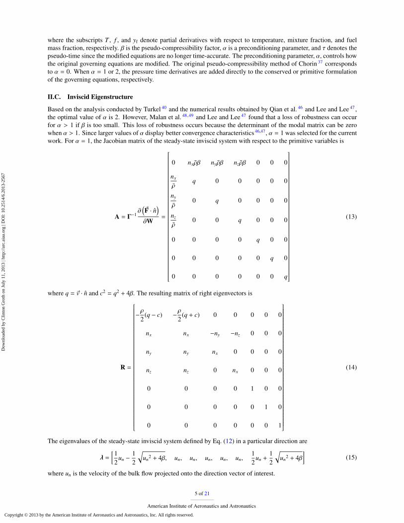
II.C. Inviscid Eigenstructure

Based on the analysis conducted by Turkel 40 and the numerical results obtained by Qian et al. 46 and Lee and Lee 47 ,the optimal value of α is 2. However, Malan et al. 48,49 and Lee and Lee 47 found that a loss of robustness can occurfor α > 1 if β is too small. This loss of robustness occurs because the determinant of the modal matrix can be zerowhen α > 1. Since larger values of α display better convergence characteristics46,47, α = 1 was selected for the currentwork. For α = 1, the Jacobian matrix of the steady-state inviscid system with respect to the primitive variables is

A = Γ−1∂(~F · n

)∂W

=

0 nxρβ nyρβ nzρβ 0 0 0

nx

ρq 0 0 0 0 0

ny

ρ0 q 0 0 0 0

nz

ρ0 0 q 0 0 0

0 0 0 0 q 0 0

0 0 0 0 0 q 0

0 0 0 0 0 0 q

(13)

where q = ~v · n and c2 = q2 + 4β. The resulting matrix of right eigenvectors is

R =

−ρ

2(q − c) −

ρ

2(q + c) 0 0 0 0 0

nx nx −ny −nz 0 0 0

ny ny nx 0 0 0 0

nz nz 0 nx 0 0 0

0 0 0 0 1 0 0

0 0 0 0 0 1 0

0 0 0 0 0 0 1

(14)

The eigenvalues of the steady-state inviscid system defined by Eq. (12) in a particular direction are

λ =

[12

un −12

√un

2 + 4β, un, un, un, un, un,12

un +12

√un

2 + 4β]

(15)

where un is the velocity of the bulk flow projected onto the direction vector of interest.

5 of 21


Dow

nloa

ded

by C

linto

n G

roth

on

July

11,

201

3 | h

ttp://

arc.

aiaa

.org

| D

OI:

10.

2514

/6.2

013-

2567


The minimum value of β was chosen based on the following formulation proposed by Turkel 40 :

β = max[2(u2 + v2 + w2

), ε

](16)

where ε is a smallness parameter.

III. CENO Finite-Volume Scheme

In the proposed cell-centered finite-volume approach, the physical domain is discretized into finite-sized compu-tational cells and the integral forms of conservation laws are applied to each individual cell. For a cell i, the approachresults in the following coupled system of partial differential equations (PDEs) for cell-averaged solution quantities:

dUi

dt+ Γi

dWi

dτ= −

1Vi

(~F − ~Fv

)· n dA +

1Vi

$S dV = −Ri (17)

where the overbar denotes cell-averaged quantities, V is the cell volume, A is the area of the face and n is the unitvector normal to a given face. Applying Gauss quadrature to evaluate the surface and volume integrals in Eq. (17)produces a set of nonlinear ordinary differential equations (ODEs) given by

dUi

dt+ Γi

dWi

dτ= −

1Vi

Nf∑l=1

NGf∑m=1

[ωf

(~F − ~Fv

)· nA

]i,l,m

+1Vi

NGv∑n=1

[ωvSV]i,n (18)

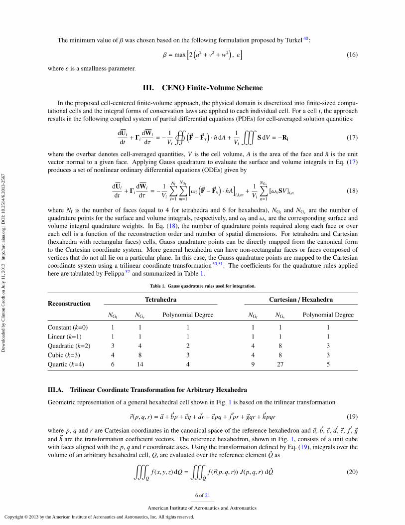
where Nf is the number of faces (equal to 4 for tetrahedra and 6 for hexahedra), NGf and NGv are the number ofquadrature points for the surface and volume integrals, respectively, and ωf and ωv are the corresponding surface andvolume integral quadrature weights. In Eq. (18), the number of quadrature points required along each face or overeach cell is a function of the reconstruction order and number of spatial dimensions. For tetrahedra and Cartesian(hexahedra with rectangular faces) cells, Gauss quadrature points can be directly mapped from the canonical formto the Cartesian coordinate system. More general hexahedra can have non-rectangular faces or faces composed ofvertices that do not all lie on a particular plane. In this case, the Gauss quadrature points are mapped to the Cartesiancoordinate system using a trilinear coordinate transformation50,51. The coefficients for the quadrature rules appliedhere are tabulated by Felippa 52 and summarized in Table 1.

Table 1. Gauss quadrature rules used for integration.

Reconstruction Tetrahedra Cartesian / Hexahedra

NGf NGv Polynomial Degree NGf NGv Polynomial Degree

Constant (k=0) 1 1 1 1 1 1Linear (k=1) 1 1 1 1 1 1Quadratic (k=2) 3 4 2 4 8 3Cubic (k=3) 4 8 3 4 8 3Quartic (k=4) 6 14 4 9 27 5

III.A. Trilinear Coordinate Transformation for Arbitrary Hexahedra

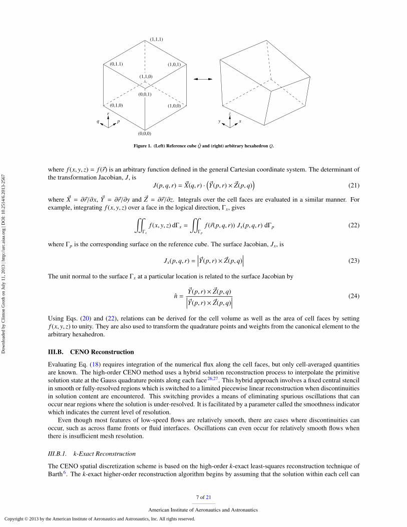
Geometric representation of a general hexahedral cell shown in Fig. 1 is based on the trilinear transformation

~r(p, q, r) = ~a + ~bp + ~cq + ~dr + ~epq + ~f pr + ~gqr + ~hpqr (19)

where p, q and r are Cartesian coordinates in the canonical space of the reference hexahedron and ~a, ~b, ~c, ~d, ~e, ~f , ~gand ~h are the transformation coefficient vectors. The reference hexahedron, shown in Fig. 1, consists of a unit cubewith faces aligned with the p, q and r coordinate axes. Using the transformation defined by Eq. (19), integrals over thevolume of an arbitrary hexahedral cell, Q, are evaluated over the reference element Q as$

Qf (x, y, z) dQ =

$Q

f (~r(p, q, r)) J(p, q, r) dQ (20)

6 of 21


Dow

nloa

ded

by C

linto

n G

roth

on

July

11,

201

3 | h

ttp://

arc.

aiaa

.org

| D

OI:

10.

2514

/6.2

013-

2567


r

pq y x

z

(0,0,0)

(0,1.1) (1,0,1)

(1,0,0)(0,1,0)

(1,1,1)

(0,0,1)

(1,1,0)

Figure 1. (Left) Reference cube Q and (right) arbitrary hexahedron Q.

where f (x, y, z) = f (~r) is an arbitrary function defined in the general Cartesian coordinate system. The determinant ofthe transformation Jacobian, J, is

J(p, q, r) = ~X(q, r) ·(~Y(p, r) × ~Z(p, q)

)(21)

where ~X = ∂~r/∂x, ~Y = ∂~r/∂y and ~Z = ∂~r/∂z. Integrals over the cell faces are evaluated in a similar manner. Forexample, integrating f (x, y, z) over a face in the logical direction, Γx, gives"

Γx

f (x, y, z) dΓx =

"Γp

f (~r(p, q, r)) Jx(p, q, r) dΓp (22)

where Γp is the corresponding surface on the reference cube. The surface Jacobian, Jx, is

Jx(p, q, r) =∣∣∣∣~Y(p, r) × ~Z(p, q)

∣∣∣∣ (23)

The unit normal to the surface Γx at a particular location is related to the surface Jacobian by

n =~Y(p, r) × ~Z(p, q)∣∣∣∣~Y(p, r) × ~Z(p, q)

∣∣∣∣ (24)

Using Eqs. (20) and (22), relations can be derived for the cell volume as well as the area of cell faces by settingf (x, y, z) to unity. They are also used to transform the quadrature points and weights from the canonical element to thearbitrary hexahedron.

III.B. CENO Reconstruction

Evaluating Eq. (18) requires integration of the numerical flux along the cell faces, but only cell-averaged quantitiesare known. The high-order CENO method uses a hybrid solution reconstruction process to interpolate the primitivesolution state at the Gauss quadrature points along each face26,27. This hybrid approach involves a fixed central stencilin smooth or fully-resolved regions which is switched to a limited piecewise linear reconstruction when discontinuitiesin solution content are encountered. This switching provides a means of eliminating spurious oscillations that canoccur near regions where the solution is under-resolved. It is facilitated by a parameter called the smoothness indicatorwhich indicates the current level of resolution.

Even though most features of low-speed flows are relatively smooth, there are cases where discontinuities canoccur, such as across flame fronts or fluid interfaces. Oscillations can even occur for relatively smooth flows whenthere is insufficient mesh resolution.

III.B.1. k-Exact Reconstruction

The CENO spatial discretization scheme is based on the high-order k-exact least-squares reconstruction technique ofBarth6. The k-exact higher-order reconstruction algorithm begins by assuming that the solution within each cell can

7 of 21


Dow

nloa

ded

by C

linto

n G

roth

on

July

11,

201

3 | h

ttp://

arc.

aiaa

.org

| D

OI:

10.

2514

/6.2

013-

2567


be represented by the following Taylor series expansion in three dimensions:

uki (x, y, z) =

(p1+p2+p3)≤k∑p1=0

∑p2=0

∑p3=0

(x − xi)p1 (y − yi)p2 (z − zi)p3 Dp1 p2 p3 (25)

where uki is the reconstructed solution quantity, (xi,yi,zi) are the coordinates of the cell centroid, k is the degree of

the piecewise polynomial interpolant and Dp1 p2 p3 are the unknown coefficients of the Taylor series expansion. Thesummation indices, p1, p2 and p3, must always satisfy the condition that (p1 + p2 + p3) ≤ k.

The following conditions are applied to determine the unknown coefficients: i) the solution reconstruction mustreproduce polynomials of degree N ≤ k exactly; ii) the mean or average value within the computational cell must bepreserved; and iii) the reconstruction must have compact support. The second condition states that

ui =1Vi

$Vi

uki (x, y, z) dV (26)

where ui is the cell average.The third condition dictates the number and location of neighboring cells included in the reconstruction. For a

compact stencil, the minimum number of neighbors is equal to the number of unknowns minus one (because of theconstraint imposed by Eq. (26)). For any type of mesh, the total number of unknown coefficients for a particular orderis given by

N =1d!

d∏n=1

(k + n) (27)

where d represents the number of space dimensions. In three-dimensions, there are four, ten, twenty and thirty-fiveunknown coefficients for k=1, k=2, k=3 and k=4, respectively. Additional neighbors are included to ensure that thestencil is not biased in any particular direction and that the reconstruction remains reliable on poor quality mesheswith high aspect ratio cells26. For each neighboring cell, p, a constraint is formed by requiring that

up =1

Vp

$Vp

uki (x, y, z) dV (28)

Since the constraints of Eqs. (26) and (28) result in an over-determined system of linear equations, a least-squaressolution for the coefficients, Dp1 p2 p3 , is obtained in each cell. Equation (26) is strictly enforced by Gaussian eliminationand a minimum-error solution to the remaining constraint equations is sought. Substituting Eq. (25) into Eq. (26) andrearranging for D000 gives

D000 = ui −

(p1+p2+p3)≤k∑∑∑(p1+p2+p3)>0

Dp1 p2 p3

1Vi

$Vi

(x − xi)p1 (y − yi)p2 (z − zi)p3 dV (29)

A similar relation is obtained using Eqs. (25) and (28) to give

D000 = u j −

(p1+p2+p3)≤k∑∑∑(p1+p2+p3)>0

Dp1 p2 p3

1V j

$V j

(x − xi)p1 (y − yi)p2 (z − zi)p3 dV (30)

Equating Eq. (29) and Eq. (30) gives

u j − ui =

(p1+p2+p3)≤k∑∑∑(p1+p2+p3)>0

Dp1 p2 p3(xp1 yp2 zp3 )i j (31)

where

(xp1 yp2 zp3 )i j =1V j

$V j

(x − xi)p1 (y − yi)p2 (z − zi)p3 dV −1Vi

$Vi

(x − xi)p1 (y − yi)p2 (z − zi)p3 dV (32)

8 of 21


Dow

nloa

ded

by C

linto

n G

roth

on

July

11,

201

3 | h

ttp://

arc.

aiaa

.org

| D

OI:

10.

2514

/6.2

013-

2567


are geometric coefficients which only depend on the mesh geometry. The new overdetermined linear system is formedusing Eq. (31) and given by

(x0y0z1)i1 · · · (xp1 yp2 zp3 )i1 · · · (xky0z0)i1...

......(x0y0z1)i j · · · (xp1 yp2 zp3 )i j · · · (xky0z0)i j

......

...(x0y0z1)iNn· · · (xp1 yp2 zp3 )iNn

· · · (xky0z0)iNn

·

D001...

Dp1 p2 p3

...

Dk00

=

u1 − ui...

u j − ui...

uNn − ui

(33)

where Nn is the number of neighbors in the stencil. The remaining polynomial coefficient, D000, is obtained fromEq. (29) after obtaining the least-squares solution to the overdetermined system given by Eq. (33).

The resulting coefficient matrix of the linear system defined in Eq. (33) depends only on the mesh geometry, so itcan be inverted and stored prior to computations14,53. Either a Householder QR factorization algorithm or orthogonaldecomposition by the SVD method was used to solve the weighted least-squares problem54. Weighting is applied hereto each individual constraint equation to improve the locality of the reconstruction55. An inverse distance weightingformula is applied. For the reconstruction in cell i,

w j =1

|~x j − ~xi|, (34)

where ~x j is the centroid of the neighbor cell j.

III.B.2. Reconstruction at Boundaries

To enforce conditions at physical boundaries, the least-squares reconstruction was constrained in adjacent controlvolumes without altering the reconstruction order of accuracy14,15,27. Constraints are placed on the least-squaresreconstruction for each variable to obtain the desired value/gradient (Dirichlet/Neumann) at each Gauss integrationpoint. Here we implement them as Robin boundary conditions

f(~x)

= a(~x)

fD(~x)

+ b(~x)

fN(~x)

(35)

where a(~x)

and b(~x)

define the contribution of the Dirichlet, fD(~x), and Neumann, fN

(~x), components, respectively.

In terms of the cell reconstruction, the Dirichlet condition is simply expressed as

fD(~xg

)= uk

(~xg

)(36)

where ~xg is the location of the Gauss quadrature point. The Neumann condition is

fN(~xg

)= ∇uk

(~xg

)· ng

=

(p1+p2+p3)≤k∑∑∑p1+p2+p3=1

∆xp1−1∆yp2−1∆zp3−1[p1∆y∆znx + p2∆x∆yny + p3∆x∆ynz

]Dp1 p2 p3 (37)

where ∆(·) = (·)g − (·)i, the subscript i denotes the location of the centroid of the cell adjacent to the boundary and gdenotes the Gauss quadrature point.

Exact solutions to the boundary constraints described by Eq. (35) are sought, which adds linear equality constraintsto the original least-squares problem (Section III.B.1). Gaussian elimination with full pivoting is first applied to removethese additional boundary constraints and the remaining least-squares problem is solved as described in Section III.B.1.

For inflow/outflow or farfield-type boundary conditions where the reconstructed variables are not related, theconstraints may be applied separately to each variable. Thus, a separate least-squares problem with equality constraintscan be set up for each variable and solved independently of the other variables. More complex boundary conditionsinvolving linear combinations of solution variables, such as symmetry or inviscid solid walls (where ~v · n = 0), cancause the reconstruction coefficients in Eq. (25) for different variables to become coupled. For these types of coupledboundary conditions, the reconstruction for all of the coupled solution variables is performed together15,27. Thus thefinal matrix in Eq. (33) for the constrained least-squares reconstruction contains the individual constraints for eachvariable (Eq. (35)), the relational constraints, and the approximate mean conservation equations for each variable(Eq. (31)).

9 of 21


Dow

nloa

ded

by C

linto

n G

roth

on

July

11,

201

3 | h

ttp://

arc.

aiaa

.org

| D

OI:

10.

2514

/6.2

013-

2567


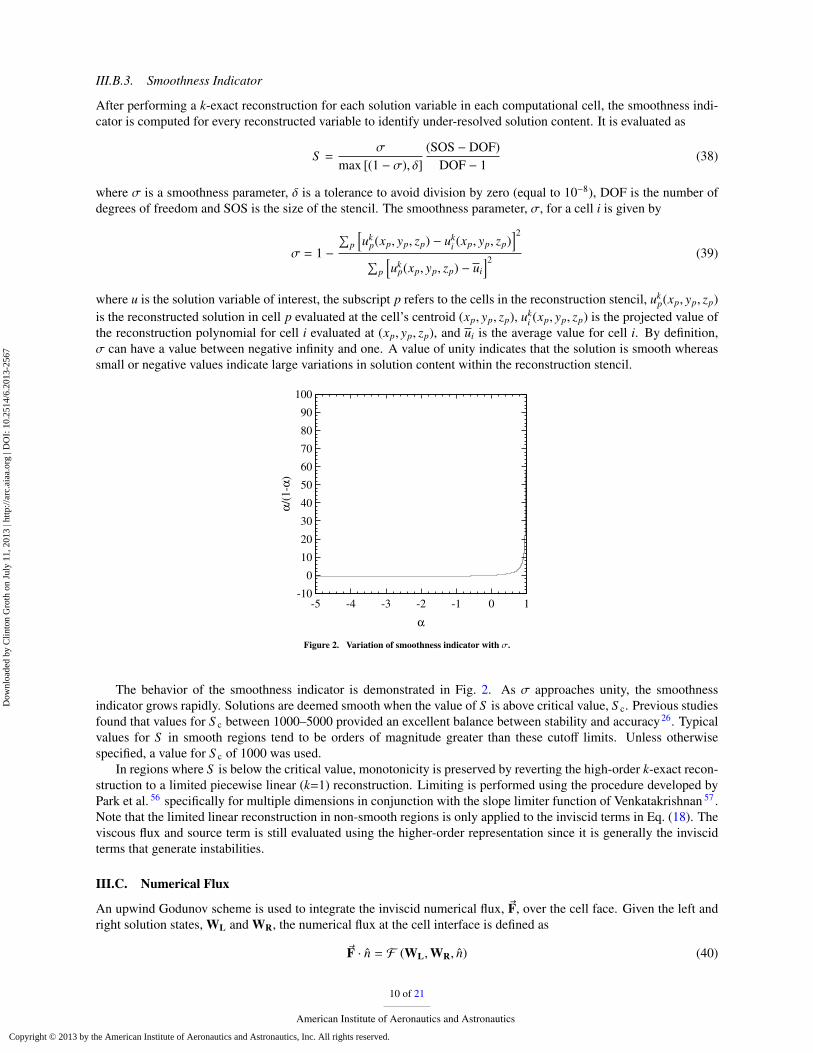
III.B.3. Smoothness Indicator

After performing a k-exact reconstruction for each solution variable in each computational cell, the smoothness indi-cator is computed for every reconstructed variable to identify under-resolved solution content. It is evaluated as

S =σ

max [(1 − σ), δ](SOS − DOF)

DOF − 1(38)

where σ is a smoothness parameter, δ is a tolerance to avoid division by zero (equal to 10−8), DOF is the number ofdegrees of freedom and SOS is the size of the stencil. The smoothness parameter, σ, for a cell i is given by

σ = 1 −

∑p

[uk

p(xp, yp, zp) − uki (xp, yp, zp)

]2

∑p

[uk

p(xp, yp, zp) − ui

]2 (39)

where u is the solution variable of interest, the subscript p refers to the cells in the reconstruction stencil, ukp(xp, yp, zp)

is the reconstructed solution in cell p evaluated at the cell’s centroid (xp, yp, zp), uki (xp, yp, zp) is the projected value of

the reconstruction polynomial for cell i evaluated at (xp, yp, zp), and ui is the average value for cell i. By definition,σ can have a value between negative infinity and one. A value of unity indicates that the solution is smooth whereassmall or negative values indicate large variations in solution content within the reconstruction stencil.

-10

0

10

20

30

40

50

60

70

80

90

100

-5 -4 -3 -2 -1 0 1

α/(1-α)

α

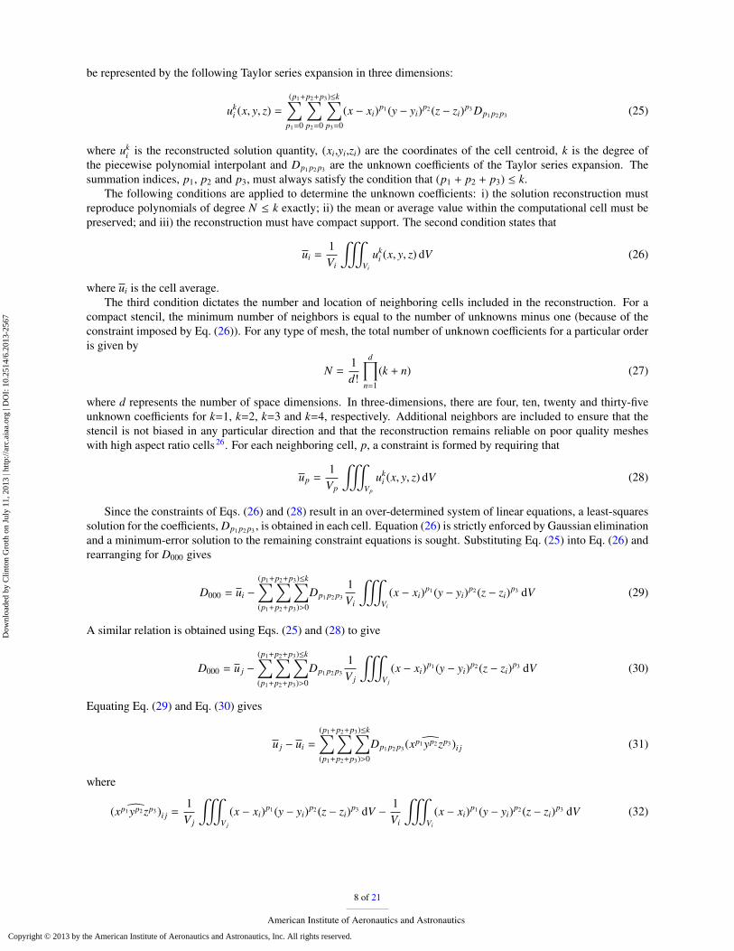
Figure 2. Variation of smoothness indicator with σ.

The behavior of the smoothness indicator is demonstrated in Fig. 2. As σ approaches unity, the smoothnessindicator grows rapidly. Solutions are deemed smooth when the value of S is above critical value, S c. Previous studiesfound that values for S c between 1000–5000 provided an excellent balance between stability and accuracy26. Typicalvalues for S in smooth regions tend to be orders of magnitude greater than these cutoff limits. Unless otherwisespecified, a value for S c of 1000 was used.

In regions where S is below the critical value, monotonicity is preserved by reverting the high-order k-exact recon-struction to a limited piecewise linear (k=1) reconstruction. Limiting is performed using the procedure developed byPark et al. 56 specifically for multiple dimensions in conjunction with the slope limiter function of Venkatakrishnan 57 .Note that the limited linear reconstruction in non-smooth regions is only applied to the inviscid terms in Eq. (18). Theviscous flux and source term is still evaluated using the higher-order representation since it is generally the inviscidterms that generate instabilities.

III.C. Numerical Flux

An upwind Godunov scheme is used to integrate the inviscid numerical flux, ~F, over the cell face. Given the left andright solution states, WL and WR, the numerical flux at the cell interface is defined as

~F · n = F (WL,WR, n) (40)

10 of 21


Dow

nloa

ded

by C

linto

n G

roth

on

July

11,

201

3 | h

ttp://

arc.

aiaa

.org

| D

OI:

10.

2514

/6.2

013-

2567


where F is a flux function which solves a Riemann problem, R, in a direction aligned along the face normal, n. Theleft and right solution states at the interface are determined using the k-exact reconstruction procedure described inSection III.B. As a result, the leading truncation error due to the inviscid operator is O

(∆xk+1

).

The flux function, F , was derived by applying Roe’s approximate Riemann solver58,59 to the new modified inviscideigensystem for Eq. (12). The numerical flux at the interface between two cells is given by

F (R (WL,WR)) =12

(FR + FL) −12|A|∆W (41)

where FL and FR are the inviscid fluxes evaluated based on WL and WR, ∆W = WR −WL, |A| = R|Λ|R−1, R isthe matrix of primitive variable right eigenvectors and Λ is the eigenvalue matrix. The matrix A is the linearized fluxJacobian evaluated at a reference state, W. A simple arithmetic average between the left and right states was chosenas the reference state.

The viscous fluxes at each quadrature point are evaluated by averaging the interface state and gradients

G (WL,WR,∇WL,∇WR) = Fv

{12

(WL + WR) ,12

(∇WL,∇WR)}

(42)

Because derivatives of the reconstructed polynomial are required, the leading truncation error due to the viscousoperator is only O

(∆xk

). The degree of the reconstruction polynomial is therefore increased by one to match the

leading truncation error introduced by the inviscid operator. The Gauss quadrature rule is selected to maintain an orderof accuracy of k + 1 when integrating the fluxes over the cell faces.

For piecewise-linear (k = 1) representations, second-order (k +1) accuracy of the viscous operator can be achievedwithout increasing the degree of the polynomial interpolatant. In this case, the average gradient at the interface isevaluated by60

∇Wi+1/2 =(Wn −Wp

) nn · ~rpn

+

(∇W − ∇W · ~rpn

nn · ~rpn

)(43)

where Wn and Wp are the solutions at the center of the two adjacent cells, and ~rpn = ~xn − ~xp is the vector between theneighboring cell centers. The weighted average of the neighboring cell gradients, ∇W, is evaluated as

∇W = χ∇Wp + (1 − χ)∇Wn (44)χ = Vp/(Vp + Vn)

Equation (43) is second-order accurate if the gradient representation is also second-order accurate. Thus, k + 1 recon-struction is not required for k = 1.

III.D. Dual-Time Stepping Approach for Unsteady Problems

Integration of the governing equations is performed in parallel to fully take advantage of modern computer architec-tures. This is carried out by dividing the computational domain up using a parallel graph partitioning algorithm, calledParmetis61, and distributing the computational cells among the available processors. Solutions for each computationalsub-domain are simultaneously computed on each processor. The proposed computational algorithm was implementedusing the message passing interface (MPI) library and the Fortran 90 programming language62. Ghost cells, whichsurround an individual local solution domain and overlap cells on neighboring domains, are used to share solutioncontent through inter-block communication.

Newton’s method is applied in this work for transient continuation using a dual-time-stepping approach41–45 withthe family of high-order backwards difference formulas to discretize the physical time derivative. Newton’s method isused to relax

R∗(W) = R +dWdt

= 0 (45)

at each physical time level. This particular implementation follows the algorithm developed by Groth et al.63–65

specifically for use on large multi-processor parallel clusters.Applying the BDF temporal discretization and Newton’s method to the semi-discrete form of the governing equa-

tions, Eq. (45), gives a∆tn

(∂U∂W

)(n+1,k)

+Γ

∆τk +

(∂R∂W

)(n+1,k) ∆W(n+1,k) = −R(n+1,k) −dUdt

∣∣∣∣∣∣(n+1,k)

= −R∗(n+1,k) (46)

11 of 21


Dow

nloa

ded

by C

linto

n G

roth

on

July

11,

201

3 | h

ttp://

arc.

aiaa

.org

| D

OI:

10.

2514

/6.2

013-

2567


where n is the outer time level, k is the now the inner iteration level, and a is a constant which depends on the temporaldiscretization (a = 1 for implicit Euler, 3/2 for BDF2, 11/6 for BDF3 and 25/12 for BDF4). Since Newton’s methodcan fail when initial solution estimates fall outside the radius of convergence, an implicit Euler discretization wasapplied to the pseudo-time term in Eq. (46).

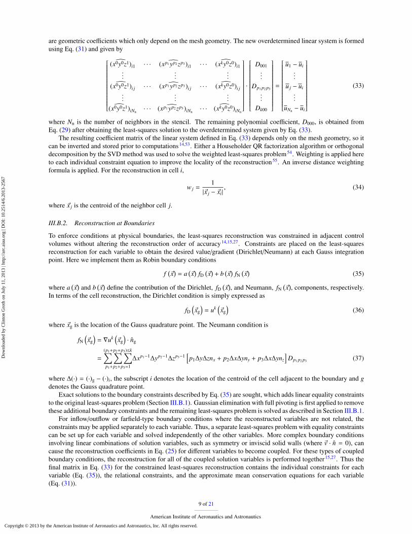
Coefficients for the different BDF schemes are provided in Table 2. The order of accuracy of the temporal dis-cretization scheme was chosen to match the accuracy of the spatial discretization. Note however, it is well known thatBDF methods with accuracy higher than second-order can be unstable when the real component of the eigenvalues ofthe system are negative. A stability analysis of the BDF methods applied to the one-dimensional form of the linearadvection equation is shown in Fig. 3. The eigenvalues, λ, for a first-order upwind discretization applied to this systemwith uniform mesh spacing ∆x and periodic boundary conditions are also shown in Fig. 3. BDF4 is stable for a CFL,ν = a∆t/∆x, up to 2. This condition may be relaxed for systems involving diffusion and relaxation processes sincethey tend to shift the eigenvalues further into the negative portion of the real λ∆t-plane. As such, the BDF methodsare still suitable for the present application since Eq. (12) involves a system of advection-diffusion-reaction equations.No issues related to the stability of the BDF methods were encountered throughout this research.

Table 2. Coefficients for the BDF methods.

bn+1un+1 + bnun + . . . = ∆t f n+1

Order un+1 un un−1 un−2 un−3

1 1 -1

2 23 −2 1

2

3 116 −3 3

2 − 13

4 2512 −4 3 4

314

−4 −2 0 2 4 6 8 10−8

−6

−4

−2

0

2

4

6

8

Re(λ∆t)

Im(λ∆t)

BDF1

BDF2

BDF3

BDF4

ν=2

ν=1

Stable

∂u

∂t+ a

∂u

∂x= 0

Figure 3. Stability diagram for the BDF methods applied to the linear advection equation. Lines enclose the unstable regions for each method; symbols are theeigenvalues for a first-order upwind spatial discretization with uniform mesh spacing ∆x and periodic boundaries. λ represents the eigenvalues, ∆t is the timestep size, a is the wave speed, and ν = a∆t/∆x is the CFL number.

In Eq. (46), ∆τk is the inner pseudo time step while ∆tn is the physical time step. The pseudo time step size wasdetermined by considering the inviscid Courant-Friedrichs-Lewy (CFL) and viscous Von Neumann stability criteriabased on the steady pseudo-compressible system. The maximum permissible time step for each local cell is determinedby

∆τk ≤ CFL ·min[

∆xmax(λ)

,ρ∆x2

µ

](47)

where CFL is a constant greater than zero which determines the time step size and ∆x = V1/3 is a measure of the gridsize. A value for CFL of 103 is typically used. The stability of the unsteady system is governed by the physical time

12 of 21


Dow

nloa

ded

by C

linto

n G

roth

on

July

11,

201

3 | h

ttp://

arc.

aiaa

.org

| D

OI:

10.

2514

/6.2

013-

2567


step size, which is determined based on the physical CFL criterion:

∆tn ≤ CFLphys ·min(

∆xu2 + v2 + w2

)(48)

where the CFLphys is the physical CFL number.

III.D.1. Inexact Newton Method

In the dual time-stepping procedure, at each physical time step n, a steady problem is solved using a Newton procedure.A solution to Eq. (46) is sought by iteratively solving a sequence of linear systems given an initial estimate, W(n+1,0),at the beginning of each physical time step. Successively improved estimates are obtained by solving(

∂R∗

∂W

)(n+1,k)

∆W(n+1,k) = J(W(n+1,k)) ∆W(n+1,k) = −R∗(W(n+1,k)) (49)

where J = ∂R∗/∂W is the residual Jacobian. After solving Eq. (49) for ∆W(n+1,k), the improved solution at step(n + 1, k) is determined from

W(n+1,k+1) = W(n+1,k) + ∆W(n+1,k) (50)

The Newton iterations proceed at each physical time level until some desired reduction of the norm of the residual isachieved and the condition ‖R∗(W(n+1,k))‖ < ε‖R∗(W(n+1,0))‖ is met. The tolerance, ε, used in this work was 10−2.

For a system of nonlinear equations, each step of Newton’s method requires the solution of the linear problemJ∆W = −R∗(W). This system tends to be relatively large, sparse, and non-symmetric for which iterative methodshave proven much more effective than direct methods. One effective method for a large variety of problems, which isused here, is the generalized minimal residual (GMRES) technique of Saad and co-workers66–69. This is an Arnoldi-based solution technique which generates orthogonal bases of the Krylov subspace to construct the solution. Thetechnique is particularly attractive because the matrix J does not need to be explicitly formed and instead only matrix-vector products are required at each iteration to create new trial vectors. This drastically reduces the required storage.Another advantage is that iterations are terminated based on only a by-product estimate of the residual which does notrequire explicit construction of the intermediate residual vectors or solutions. Termination also generally only requiressolving the linear system to some specified tolerance, ‖R∗k + Jk∆Wk‖2 < ζ‖R∗(Wk)‖2, where ζ is typically in therange 0.1 − 0.570. We use a restarted version of the GMRES algorithm here, GMRES(m), that minimizes storage byrestarting every m iterations.

Right preconditioning of J is performed to help facilitate the solution of the linear system without affecting thesolution residual, b. The preconditioning takes the form(

JM−1)

(Mx) = b (51)

where M is the preconditioning matrix. A combination of an additive Schwarz global preconditioner and a blockincomplete lower-upper (BILU) local preconditioner is used. In additive Schwarz preconditioning, the solution ineach block is updated simultaneously and shared boundary data is not updated until a full cycle of updates has beenperformed on all domains. The preconditioner is defined as follows

M−1 =

Nb∑k=1

BTk M−1

k Bk (52)

where Nb is the number of blocks and Bk is the gather matrix for the kth domain. The local preconditioner, M−1k , in

Eq. (52) is based on block ILU(p) factorization69 of the Jacobian for the first order approximation of each domain.The level of fill, p, was maintained between 0–1 to reduce storage requirements. Larger values of p typically offerimproved convergence characteristics for the linear system at the expense of storage. To further reduce computationalstorage, reverse Cuthill-McKee matrix reordering is used to permute the Jacobian’s sparsity pattern into a band matrixform with a small bandwith71.

IV. Results For Three-Dimensional Unstructured Mesh

The proposed finite-volume scheme was assessed in terms of both accuracy and stability through its application toa laboratory-scale turbulent premixed flame. All computations were performed on a high performance parallel cluster

13 of 21


Dow

nloa

ded

by C

linto

n G

roth

on

July

11,

201

3 | h

ttp://

arc.

aiaa

.org

| D

OI:

10.

2514

/6.2

013-

2567


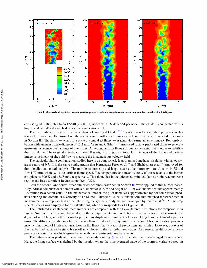
Figure 4. Measured and predicted instantaneous temperature contours. Instantaneous experimental results are unfiltered in this figure.

consisting of 3,780 Intel Xeon E5540 (2.53GHz) nodes with 16GB RAM per node. The cluster is connected with ahigh speed InfiniBand switched fabric communications link.

The lean turbulent premixed methane flame of Yuen and Gülder 72,73 was chosen for validation purposes in thisresearch. It was modelled using both the second- and fourth-order numerical schemes that were described previouslyin Section III. The flame — which is a piloted, conical jet flame — is generated using an axisymmetric Bunsen-typeburner with an inner nozzle diameter of 11.2 mm. Yuen and Gülder 72,73 employed various perforated plates to generateupstream turbulence over a range of intensities. A co-annular pilot flame surrounds the central jet in order to stabilizethe main flame. The original investigators used Rayleigh scatting to capture planar images of the flame and particleimage velocimetry of the cold flow to measure the instantaneous velocity field.

The particular flame configuration studied here is an atmospheric lean premixed methane-air flame with an equiv-alence ratio of 0.7. It is the same configuration that Hernández-Pérez et al. 74 and Shahbazian et al. 75 employed fortheir detailed numerical analysis. The turbulence intensity and length scale at the burner exit are u′/sL = 14.38 andL = 1.79 mm, where sL is the laminar flame speed. The temperature and mean velocity of the reactants at the burnerexit plane is 300 K and 15.58 m/s, respectively. This flame lies in the thickened wrinkled flame or thin reaction zoneregime and has a turbulent Reynolds number of 324.

Both the second- and fourth-order numerical schemes described in Section III were applied to this bunsen flame.A cylindrical computational domain with a diameter of 0.05 m and height of 0.1 m was subdivided into approximately1.8 million hexahedral cells. In the mathematical model, the pilot flame was approximated by hot combustion prod-ucts entering the domain at a velocity of 16.81 m/s. Turbulent velocity fluctuations that matched the experimentalmeasurements were prescribed at the inlet using the synthetic eddy method developed by Jarrin et al. 76 . A time stepsize of 12.5 µs was employed for all calculations, which corresponds to a CFLphys ≈ 0.8.

The unfiltered instantaneous measurements are compared with the Favre-filtered predictions for temperature inFig. 4. Similar structures are observed in both the experiments and predictions. The predictions underestimate thedegree of wrinkling, with the 2nd-order predictions displaying significantly less wrinkling than the 4th-order predic-tions. The 4th-order predictions have a thicker flame front and display more penetration of hot combustion productsinto the inner core of fresh reactants. Low in the flame, the two sets of predictions are similar. However, pockets offresh unburned reactants begin to break off much lower in the 4th-order predictions. As a result, the 4th-order schemepredicts a shorter flame which agrees better with the experimental measurements.

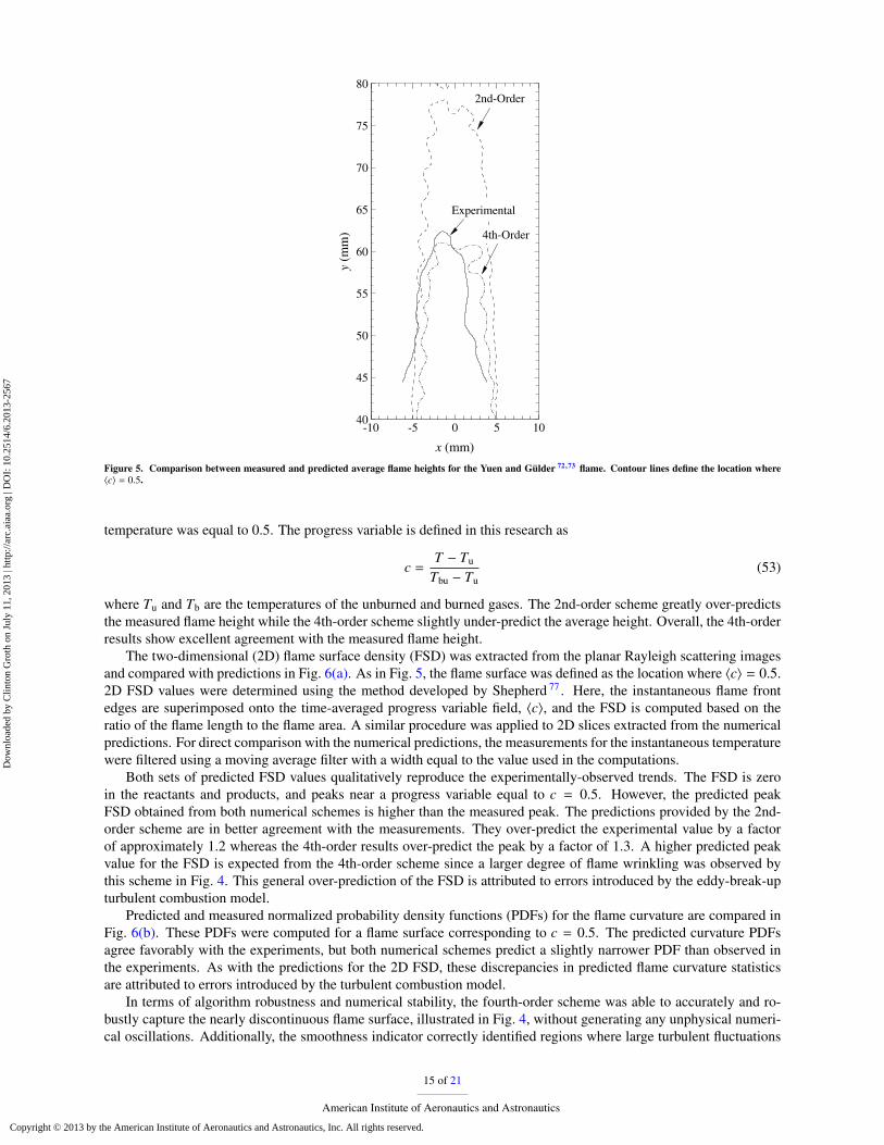
The differences in predicted flame height are evident in Fig. 5, which illustrates the time-averaged flame surface.Here, the flame surface was defined by the location where the time-averaged value of the progress variable based on

14 of 21


Dow

nloa

ded

by C

linto

n G

roth

on

July

11,

201

3 | h

ttp://

arc.

aiaa

.org

| D

OI:

10.

2514

/6.2

013-

2567


x (mm)

y (

mm

)

10 5 0 5 1040

45

50

55

60

65

70

75

80

Experimental

2ndOrder

4thOrder

Figure 5. Comparison between measured and predicted average flame heights for the Yuen and Gülder 72,73 flame. Contour lines define the location where〈c〉 = 0.5.

temperature was equal to 0.5. The progress variable is defined in this research as

c =T − Tu

Tbu − Tu(53)

where Tu and Tb are the temperatures of the unburned and burned gases. The 2nd-order scheme greatly over-predictsthe measured flame height while the 4th-order scheme slightly under-predict the average height. Overall, the 4th-orderresults show excellent agreement with the measured flame height.

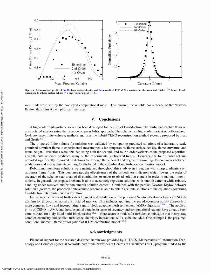
The two-dimensional (2D) flame surface density (FSD) was extracted from the planar Rayleigh scattering imagesand compared with predictions in Fig. 6(a). As in Fig. 5, the flame surface was defined as the location where 〈c〉 = 0.5.2D FSD values were determined using the method developed by Shepherd 77 . Here, the instantaneous flame frontedges are superimposed onto the time-averaged progress variable field, 〈c〉, and the FSD is computed based on theratio of the flame length to the flame area. A similar procedure was applied to 2D slices extracted from the numericalpredictions. For direct comparison with the numerical predictions, the measurements for the instantaneous temperaturewere filtered using a moving average filter with a width equal to the value used in the computations.

Both sets of predicted FSD values qualitatively reproduce the experimentally-observed trends. The FSD is zeroin the reactants and products, and peaks near a progress variable equal to c = 0.5. However, the predicted peakFSD obtained from both numerical schemes is higher than the measured peak. The predictions provided by the 2nd-order scheme are in better agreement with the measurements. They over-predict the experimental value by a factorof approximately 1.2 whereas the 4th-order results over-predict the peak by a factor of 1.3. A higher predicted peakvalue for the FSD is expected from the 4th-order scheme since a larger degree of flame wrinkling was observed bythis scheme in Fig. 4. This general over-prediction of the FSD is attributed to errors introduced by the eddy-break-upturbulent combustion model.

Predicted and measured normalized probability density functions (PDFs) for the flame curvature are compared inFig. 6(b). These PDFs were computed for a flame surface corresponding to c = 0.5. The predicted curvature PDFsagree favorably with the experiments, but both numerical schemes predict a slightly narrower PDF than observed inthe experiments. As with the predictions for the 2D FSD, these discrepancies in predicted flame curvature statisticsare attributed to errors introduced by the turbulent combustion model.

In terms of algorithm robustness and numerical stability, the fourth-order scheme was able to accurately and ro-bustly capture the nearly discontinuous flame surface, illustrated in Fig. 4, without generating any unphysical numeri-cal oscillations. Additionally, the smoothness indicator correctly identified regions where large turbulent fluctuations

15 of 21


Dow

nloa

ded

by C

linto

n G

roth

on

July

11,

201

3 | h

ttp://

arc.

aiaa

.org

| D

OI:

10.

2514

/6.2

013-

2567


Mean Progress Variable

Fla

me

Su

rfac

e D

ensi

ty (

1/m

m)

0 0.2 0.4 0.6 0.8 10

0.1

0.2

0.3

0.4

0.5

0.6

Experiment

2ndOrder

4thOrder

Curvature (1/mm)

No

rmal

ized

Pro

bab

ilit

y

5 0 50

0.2

0.4

0.6

0.8

1Experiment

2ndOrder

4thOrder

Figure 6. Measured and predicted (a) 2D flame surface density and (b) normalized PDF of 2D curvature for the Yuen and Gülder 72,73 flame. Resultscorrespond to a flame surface defined by a progress variable of c = 0.5.

were under-resolved by the employed computational mesh. This ensured the reliable convergence of the Newton-Krylov algorithm at each physical time step.

V. Conclusions

A high-order finite-volume solver has been developed for the LES of low-Mach-number turbulent reactive flows onunstructured meshes using the pseudo-compressibility approach. The scheme is a high-order variant of cell-centered,Godunov-type, finite-volume, methods and uses the hybrid CENO reconstruction method recently proposed by Ivanand Groth26,27.

The proposed finite-volume formulation was validated by comparing predicted solutions of a laboratory-scalepremixed turbulent flame to experimental measurements for temperature, flame surface density, flame curvature, andflame height. Predictions were obtained using both the second- and fourth-order variants of the proposed algorithm.Overall, both schemes predicted many of the experimentally observed trends. However, the fourth-order schemeprovided significantly improved predictions for average flame height and degree of wrinkling. Discrepancies betweenpredictions and measurements are largely attributed to the eddy-break-up turbulent combustion model.

Robust and monotone solutions were maintained throughout this study even in regions with sharp gradients, suchas across flame fronts. This demonstrates the effectiveness of the smoothness indicator, which lowers the order ofaccuracy of the scheme near areas of discontinuities or under-resolved solution content in order to maintain mono-tonicity. In general, the proposed scheme is able to accurately represent solutions with smooth extrema while robustlyhandling under-resolved and/or non-smooth solution content. Combined with the parallel Newton-Krylov-Schwarzsolution algorithm, the proposed finite-volume scheme is able to obtain accurate solutions to the equations governinglow-Mach-number turbulent reactive flow.

Future work consists of further development and validation of the proposed Newton-Krylov-Schwarz CENO al-gorithm for three-dimensional unstructured meshes. This includes applying the pseudo-compressibility approach tomore complex flows and incorporating a multi-block adaptive mesh refinement (AMR) algorithm78–81. The applica-bility of CENO to AMR and the substantial benefits in terms of accuracy and computational savings have already beendemonstrated for body-fitted multi-block meshes26,27. More accurate models for turbulent combustion that incorporatecomplex chemistry and detailed turbulence-chemistry interactions will also be included. One example is the presumedconditional moment, flame prolongation of ILDM combustion model74,82.

Acknowledgments

Financial support for the research described herein was provided by MITACS (Mathematics of Information Tech-nology and Complex Systems) Network, part of the Networks of Centres of Excellence (NCE) program funded by the

16 of 21


Dow

nloa

ded

by C

linto

n G

roth

on

July

11,

201

3 | h

ttp://

arc.

aiaa

.org

| D

OI:

10.

2514

/6.2

013-

2567


Canadian government. This funding is gratefully acknowledged with many thanks. Computational resources for per-forming all of the calculations reported herein were provided by the SciNet High Performance Computing Consortiumat the University of Toronto and Compute/Calcul Canada through funding from the Canada Foundation for Innovation(CFI) and the Province of Ontario, Canada.

References

1. Wilcox, D. C., Turbulence Modeling for CFD, DCW Industries, 3rd ed., 2006.

2. Pope, S. B., Turbulent Flows, Cambridge University Press, 2000.

3. Pirozzoli, S., “On the spectral properties of shock-capturing schemes,” J. Comput. Phys., Vol. 219, No. 2, 2006,pp. 489–497.

4. Harten, A., Engquist, B., Osher, S., and Chakravarthy, S. R., “Uniformly high order accurate essentially non-oscillatory schemes, III,” J. Comput. Phys., Vol. 71, No. 2, 1987, pp. 231–303.

5. Coirier, W. J. and Powell, K. G., “Solution-Adaptive Cartesian Cell Approach for Viscous and Inviscid Flows,”AIAA J., Vol. 34, No. 5, May 1996, pp. 938–945.

6. Barth, T. J., “Recent Developments in High Order K-Exact Reconstruction on Unstructured Meshes,” AIAA Paper93-0668, 1993.

7. Abgrall, R., “On essentially non-oscillatory schemes on unstructured meshes: analysis and implementation,”J. Comput. Phys., Vol. 114, 1994, pp. 45–58.

8. Sonar, T., “On the construction of essentially non-oscillatory finite volume approximations to hyperbolic conserva-tion laws on general triangulations: polynomial recovery, accuracy and stencil selection,” Comp. Meth. Appl. Mech.Eng., 1997, pp. 140–157.

9. Ollivier-Gooch, C. F., “Quasi-ENO Schemes for Unstructured Meshes Based on Unlimited Data-Dependent Least-Squares Reconstruction,” J. Comput. Phys., Vol. 133, 1997, pp. 6–17.

10. Jiang, G. S. and Shu, C. W., “Efficient implementation of weighted ENO schemes,” J. Comput. Phys., Vol. 126,No. 1, 1996, pp. 202–228.

11. Stanescu, D. and Habashi, W., “Essentially Nonoscillatory Euler solutions on unstructured meshes using extrapo-lation,” AIAA J., Vol. 36, 1998, pp. 1413–1416.

12. Friedrich, O., “Weighted essentially non-oscillatory schemes for the interpolation of mean values on unstructuredgrids,” J. Comput. Phys., Vol. 144, 1998, pp. 194–212.

13. Hu, C. and Shu, C.-W., “Weighted essentially non-oscillatory schemes on triangular meshes,” J. Comput. Phys.,Vol. 150, 1999, pp. 97–127.

14. Ollivier-Gooch, C. F. and Van Altena, M., “A high-order accurate unstructured mesh finite-volume scheme for theadvection-diffusion equation,” J. Comput. Phys., Vol. 181, No. 2, 2002, pp. 729–752.

15. Nejat, A. and Ollivier-Gooch, C., “A high-order accurate unstructured finite volume Newton-Krylov algorithm forinviscid compressible flows,” J. Comput. Phys., Vol. 227, No. 4, 2008, pp. 2582–2609.

16. Cockburn, B. and Shu, C.-W., “TVB Runge-Kutta Local Projection Discontinous Galerkin Finite-Element Methodfor Conservation Laws II: General Framework,” Math. Comp., Vol. 52, 1989, pp. 411.

17. Cockburn, B., Hou, S., and Shu, C.-W., “TVB Runge-Kutta Local Projection Discontinous Galerkin Finite-Element Method for Conservation Laws IV: The Multidimensional Case,” J. Comput. Phys., Vol. 54, 1990, pp. 545.

18. Hartmann, R. and Houston, P., “Adaptive Discontinuous Galerkin Finite Element Methods for the CompressibleEuler Equations,” J. Comput. Phys., Vol. 183, 2002, pp. 508–532.

19. Luo, H., Baum, J. D., and Löhner, R., “A Hermite WENO-based limiter for discontinuous Galerkin method onunstructured grids,” J. Comput. Phys., Vol. 225, 2007, pp. 686–713.

17 of 21


Dow

nloa

ded

by C

linto

n G

roth

on

July

11,

201

3 | h

ttp://

arc.

aiaa

.org

| D

OI:

10.

2514

/6.2

013-

2567


20. Gassner, G., Lörcher, F., and Munz, C.-D., “A contribution to the construction of diffusion fluxes for finite volumeand discontinuous Galerkin schemes,” J. Comput. Phys., Vol. 224, No. 2, 2007, pp. 1049–1063.

21. Wang, Z. J., “Spectral (Finite) Volume Method for Conservation Laws on Unstructured Grids – Basic Formula-tion,” J. Comput. Phys., Vol. 178, 2002, pp. 210–251.

22. Wang, Z. J. and Liu, Y., “Spectral (Finite) Volume Method for Conservation Laws on Unstructured Grids – II.Extenstion to Two-Dimensional Scalar Equation,” J. Comput. Phys., Vol. 179, 2002, pp. 665–697.

23. Wang, Z. J., Zhang, L., and Liu, Y., “High-Order Spectral Volume Method for 2D Euler Equations,” Paper 2003–3534, AIAA, June 2003.

24. Wang, Z. J. and Liu, Y., “Spectral (Finite) Volume Method for Conservation Laws on Unstructured Grids –III. One Dimensional Systems and Partition Optimization,” Journal of Scientific Computing, Vol. 20, No. 1, 2004,pp. 137–157.

25. Sun, Y., Wang, Z. J., and Liu, Y., “Spectral (finite) volume method for conservation laws on unstructured gridsVI: extension to viscous flow,” J. Comput. Phys., Vol. 215, No. 1, 2006, pp. 41–58.

26. Ivan, L. and Groth, C. P. T., “High-order central CENO finite-volume scheme with adaptive mesh refinement,”AIAA paper 2007-4323, 2007.

27. Ivan, L. and Groth, C. P. T., “High-order solution-adaptive central essentially non-oscillatory (CENO) method forviscous flows,” AIAA paper 2011-0367, 2011.

28. Haselbacher, A., “A WENO Reconstruction Algorithm for Unstructed Grids Based on Explicit Stencil Construc-tion,” AIAA paper 2005-0879, 2005.

29. McDonald, S. D., Charest, M. R. J., and Groth, C. P. T., “High-order CENO finite-volume schemes for multi-blockunstructured mesh,” 20th AIAA Computational Fluid Dynamics Conference, Honolulu, Hawaii, June 27–30 2011,AIAA-2011-3854.

30. Charest, M. R. J., Groth, C. P. T., and Gauthier, P. Q., “High-order CENO finite-volume scheme for low-speed vis-cous flows on three-dimensional unstructured mesh,” ICCFD7 - International Conference on Computational FluidDynamics, Hawaii, July 9–13 2012, Paper ICCFD7-1002.

31. Smagorinski, J., “General Circulation Experiments with the Primitive Equations. I: The Basic Experiment,”Monthly Weather Review, Vol. 91, No. 3, 1979, pp. 99–165.

32. Magnussen, B. F. and Hjertager, B. H., “On mathematical modeling of turbulent combustion with special emphasison soot formation and combustion,” Proc. Combust. Inst., Vol. 16, No. 1, 1977, pp. 719–729.

33. Spalding, D. B., “Mixing and chemical reaction in steady confined turbulent flames,” Proc. Combust. Inst., Vol. 13,No. 1, 1971, pp. 649–657.

34. Balaras, E., Benocci, C., and Piomelli, U., “Two-layer approximate boundary conditions for large-eddy simula-tions,” AIAA J., Vol. 34, No. 6, 1996, pp. 1111–1119.

35. Piomelli, U. and Balaras, E., “Wall-layer models for large-eddy simulations,” Ann. Rev. Fluid Mech., Vol. 34,2002, pp. 349–374.

36. Driest, E. V., “On turbulent flow near a wall,” J. Appl. Sci., Vol. 23, No. 11, 1956, pp. 1007–1011.

37. Chorin, A. J., “A numerical method for solving incompressible viscous flow problems,” J. Comput. Phys., Vol. 2,No. 1, 1967, pp. 12–26.

38. Steger, J. L. and Kutler, P., “Implicit finite-difference procedures for the computation of vortex wakes,” AIAA J.,Vol. 15, No. 4, 1977, pp. 581–590.

39. Chang, S. L. and Rhee, K. T., “Blackbody radiation functions,” Int. Commun. Heat Mass Transfer, Vol. 11, No. 5,1984, pp. 451–455.

18 of 21


Dow

nloa

ded

by C

linto

n G

roth

on

July

11,

201

3 | h

ttp://

arc.

aiaa

.org

| D

OI:

10.

2514

/6.2

013-

2567


40. Turkel, E., “Preconditioned methods for solving the incompressible and low speed compressible equations,”J. Comput. Phys., Vol. 72, No. 2, 1987, pp. 277–298.

41. Jameson, A., “Time dependent calculations using multigrid, with applications to unsteady flows past airfoils andwings,” AIAA paper 1991-1596, 1991.

42. Merkle, C. L. and Athavale, M., “Time-accurate unsteady incompressible flow algorithms based on artificialcompressibility,” AIAA paper 87-1137, 1987.

43. Soh, W. Y. and Goodrich, J. W., “Unsteady solution of incompressible Navier-Stokes equations,” J. Comput. Phys.,Vol. 79, No. 1, 1988, pp. 113–134.

44. Rogers, S. E. and Kwak, D., “Upwind differencing scheme for the time-accurate incompressible Navier-Stokesequations,” AIAA J., Vol. 28, No. 2, 1990, pp. 253–262.

45. Rogers, S. E., Kwak, D., and Kiris, C., “Steady and unsteady solutions of the incompressible Navier-Stokesequations,” AIAA J., Vol. 29, No. 4, 1991, pp. 603–610.

46. Qian, Z., Zhang, J., and Li, C., “Preconditioned pseudo-compressibility methods for incompressible Navier-Stokesequations,” Science China: Physics, Mechanics and Astronomy, Vol. 53, No. 11, 2010, pp. 2090–2102.

47. Lee, H. and Lee, S., “Convergence characteristics of upwind method for modified artificial compressibilitymethod,” Int. J. Aeronaut. Space Sci., Vol. 12, No. 4, 2011, pp. 318–330.

48. Malan, A. G., Lewis, R. W., and Nithiarasu, P., “An improved unsteady, unstructured, artificial compressibility,finite volume scheme for viscous incompressible flows: Part I. Theory and implementation,” Int. J. Numer. Meth.Engin., Vol. 54, No. 5, 2002, pp. 695–714.

49. Malan, A. G., Lewis, R. W., and Nithiarasu, P., “An improved unsteady, unstructured, artificial compressibility,finite volume scheme for viscous incompressible flows: Part II. Application,” Int. J. Numer. Meth. Engin., Vol. 54,No. 5, 2002, pp. 715–729.

50. Naff, R. L., Russell, T. F., and Wilson, J. D., “Shape functions for three-dimensional control-volume mixed finite-element methods on irregular grids,” Developments in Water Science, Vol. 47, Elsevier, 2002, pp. 359–366.

51. Naff, R., Russell, T., and Wilson, J., “Shape functions for velocity interpolation in general hexahedral cells,”Computat. Geosci., Vol. 6, 2002, pp. 285–314.

52. Felippa, C. A., “A compendium of FEM integration formulas for symbolic work,” Eng. Computation., Vol. 21,No. 8, 2004, pp. 867–890.

53. Ivan, L., Development of high-order CENO finite-volume schemes with block-based adaptive mesh refinement,Ph.D. thesis, University of Toronto, 2011.

54. Lawson, C. L. and Hanson, R. J., Solving least squares problems, Prentice-Hall, 1974.

55. Mavriplis, D. J., “Revisiting the least-squares procedure for gradient reconstruction on unstructured meshes,”AIAA paper 2003-3986, 2003.

56. Park, J. S., Yoon, S.-H., and Kim, C., “Multi-dimensional limiting process for hyperbolic conservation laws onunstructured grids,” J. Comput. Phys., Vol. 229, No. 3, 2010, pp. 788–812.

57. Venkatakrishnan, V., “On the Accuracy of Limiters and Convergence to Steady State Solutions,” AIAA Paper93-0880, 1993.

58. Roe, P. L., “Approximate Riemann solvers, parameter vectors, and difference schemes,” J. Comput. Phys., Vol. 43,1981, pp. 357–372.

59. Roe, P. L. and Pike, J., “Efficient Construction and Utilisation of Approximate Riemann Solutions,” ComputingMethods in Applied Science and Engineering, edited by R. Glowinski and J. L. Lions, Vol. VI, North-Holland,Amsterdam, 1984, pp. 499–518.

19 of 21


Dow

nloa

ded

by C

linto

n G

roth

on

July

11,

201

3 | h

ttp://

arc.

aiaa

.org

| D

OI:

10.

2514

/6.2

013-

2567


60. Mathur, S. R. and Murthy, J. Y., “A pressure-based method for unstructured meshes,” Numer. Heat Transfer, PartB, Vol. 31, No. 2, 1997, pp. 195–215.

61. Karypis, G. and Schloegel, K., “ParMeTis: Parallel graph graph partitioning and sparse matrix ordering library,Version 4.0,” http://www.cs.umn.edu/~metis, 2011.

62. Gropp, W., Lusk, E., and Skjellum, A., Using MPI, MIT Press, Cambridge, Massachussets, 1999.

63. Groth, C. P. T. and Northrup, S. A., “Parallel implicit adaptive mesh refinement scheme for body-fitted multi-block mesh,” 17th AIAA Computational Fluid Dynamics Conference, Toronto, Ontario, Canada, 6-9 June 2005,AIAA paper 2005-5333.

64. Charest, M. R. J., Groth, C. P. T., and Gülder, Ö. L., “A computational framework for predicting laminar reactiveflows with soot formation,” Combust. Theor. Modelling, Vol. 14, No. 6, 2010, pp. 793–825.

65. Charest, M. R. J., Groth, C. P. T., and Gülder, Ö. L., “Solution of the equation of radiative transfer using aNewton-Krylov approach and adaptive mesh refinement,” J. Comput. Phys., Vol. 231, No. 8, 2012, pp. 3023–3040.

66. Saad, Y. and Schultz, M. H., “GMRES: A generalized minimal residual algorithm for solving nonsymmetric linearsystems,” SIAM J. Sci. Stat. Comput., Vol. 7, No. 3, 1986, pp. 856–869.

67. Saad, Y., “Krylov Subspace Methods on Supercomputers,” SIAM J. Sci. Stat. Comput., Vol. 10, No. 6, 1989,pp. 1200–1232.

68. Brown, P. N. and Saad, Y., “Hybrid Krylov Methods for Nonlinear Systems of Equations,” SIAM J. Sci. Stat.Comput., Vol. 11, No. 3, 1990, pp. 450–481.

69. Saad, Y., Iterative Methods for Sparse Linear Systems, PWS Publishing Company, Boston, 1996.

70. Dembo, R. S., Eisenstat, S. C., and Steihaug, T., “Inexact Newton Methods,” SIAM J. Numer. Anal., Vol. 19, No. 2,1982, pp. 400–408.

71. Cuthill, E. and McKee, J., “Reducing the bandwidth of sparse symmetric matrices,” Proceedings of the 1969 24thNational Conference, ACM ’69, ACM, New York, NY, USA, 1969, pp. 157–172.

72. Yuen, F. T. and Gülder, Ö. L., “Investigation of dynamics of lean turbulent premixed flames by Rayleigh imaging,”AIAA J., Vol. 47, No. 12, 2009, pp. 2964–2973.

73. Yuen, F. T. and Gülder, Ö. L., “Premixed turbulent flame front structure investigation by Rayleigh scattering inthe thin reaction zone regime,” Proc. Combust. Inst., Vol. 32, 2009, pp. 1747–1754.

74. Hernández-Pérez, F. E., Yuen, F. T. C., Groth, C. P. T., and Gülder, Ö. L., “LES of a laboratory-scale turbulentpremixed Bunsen flame using FSD, PCM-FPI and thickened flame models,” Vol. 33, 2011, pp. 1365–1371.

75. Shahbazian, N., Groth, C. P. T., and Gülder, Ö. L., “Assessment of presumed PDF models for large eddy simulationof turbulent premixed flames,” AIAA Paper 2011-0781, 2011.

76. Jarrin, N., Benhamadouche, S., Laurence, D., and Prosser, R., “A synthetic-eddy-method for generating inflowconditions for large-eddy simulations,” Int. J. of Heat Fluid Fl, Vol. 27, No. 4, 2006, pp. 585–593.

77. Shepherd, I., “Flame surface density and burning rate in premixed turbulent flames,” Proc. Combust. Inst., Vol. 26,1996, pp. 373–379.

78. Sachdev, J. S., Groth, C. P. T., and Gottlieb, J. J., “A parallel solution-adaptive scheme for multi-phase core flowsin solid propellant rocket motors,” Int. J. Comput. Fluid Dyn., Vol. 19, No. 2, 2005, pp. 159–177.

79. Gao, X. and Groth, C. P. T., “A parallel adaptive mesh refinement algorithm for predicting turbulent non-premixedcombusting flows,” Int. J. Comput. Fluid Dyn., Vol. 20, No. 5, 2006, pp. 349–357.

80. Gao, X. and Groth, C. P. T., “A parallel solution-adaptive method for three-dimensional turbulent non-premixedcombusting flows,” J. Comput. Phys., Vol. 229, No. 9, 2010, pp. 3250–3275.

20 of 21


Dow

nloa

ded

by C

linto

n G

roth

on

July

11,

201

3 | h

ttp://

arc.

aiaa

.org

| D

OI:

10.

2514

/6.2

013-

2567


http://www.cs.umn.edu/~metis

81. Gao, X., Northrup, S., and Groth, C. P. T., “Parallel solution-adaptive method for two-dimensional non-premixedcombusting flows,” Prog. Comput. Fluid. Dy., Vol. 11, No. 2, 2011, pp. 76–95.

82. Domingo, P., Vervisch, L., Payet, S., and Hauguel, R., “DNS of a premixed turbulent V flame and LES of a ductedflame using a FSD-PDF subgrid scale closure with FPI-tabulated chemistry,” Combust. Flame, Vol. 143, No. 4, 2005,pp. 566–586.

21 of 21


Dow

nloa

ded

by C

linto

n G

roth

on

July

11,

201

3 | h

ttp://

arc.

aiaa

.org

| D

OI:

10.

2514

/6.2

013-

2567


aiaa-2013-2567-charest

Documents