For permission to copy or republish, contact the American Institute of Aeronautics and Astronautics,1801 Alexander Bell Drive, Suite 500, Reston, VA 20191-4344

AIAA 2000-0272

Unsteady Separated Flow Simulationsusing a Cluster of Workstations

Anirudh Modi and Lyle N. LongThe Pennsylvania State UniversityUniversity Park, PA

38th Aerospace SciencesMeeting & Exhibit

10 – 13 January 2000 / Reno, NV

UNSTEADY SEPARATED FLOW SIMULATIONS USINGA CLUSTER OF WORKSTATIONS

Anirudh Modi� and Lyle N. Long†

Department of Aerospace EngineeringThe Pennsylvania State University

University Park, PA-16802

Abstract

The possibility of predicting the full three-dimensional,unsteady, separated flow around complex ship andhelicopter geometries is explored using unstructuredgrids in a parallel flow solver. The flow solver used is amodified version of the Parallel Unstructured MaritimeAerodynamics (PUMA) software. The efficiencyand accuracy of PUMA at resolving several steadystate solutions and a fully three-dimensional unsteadyseparated flow around a sphere were studied. Since thisrequires immense computational resources, one has tooften depend on expensive supercomputers to do thejob. TheCOst effective COmputing Array(COCOA) isan inexpensive Beowulf-class supercomputer built andtested by the Aerospace Engineering Department at thePennsylvania State University, as part of an effort tomake this possible at a very economical cost. Variousbenchmarks were conducted on COCOA to study itsperformance at solving such problems. Unstructuredgrids were utilized in order to maximize the number ofcells in the area of interest, while minimizing cells in thefar field. A high level of clustering is required to solveviscous unsteady problems, and unstructured grids offerthe least expensive method to ensure this. NASA’sVGRID package was used to generate the unstructuredgrids.

Introduction

The prediction of unsteady separated, low Machnumber flows over complex configurations (like

1� Graduate Research Assistant, Student Member† Professor, Associate Fellow

ships and helicopter fuselages) is known to bea very difficult problem. The possibility ofpredicting these types of flows with the aid ofinexpensive parallel computers is explored in thiswork. A parallel, finite volume flow solver wasused and efforts were made to expedite the entiresolution process.

An example of a separated flow around a bodywith sharp edges is the air flow around ships.The increasing use of helicopter in conjunctionwith ships poses major problems. In the presenceof high winds and rough seas, excessive shipmotions and turbulent separated flow from sharp-edged, box-like ship super-structures make landinga helicopter on ships a very hazardous operation.The strong unsteady flows can cause severe rotorblade deformations as well. Recent research onship airwakes has been conducted from severaldifferent approaches. A simple model of a ship, butrather crude, is a sharp edged blunt body called theGeneral Ship Shape (GSS).1, 2 More geometricallyprecise studies have been carried out in windtunnels3, 4 and full scale tests have been conductedby the US Navy.5 There have been severalother attempts at numerically simulating shipairwakes, but no method to-date has been entirelysatisfactory for predicting these flow fields.

Another class of problems that are somewhatsimilar to those above are the flow over bluffbodies such as helicopter fuselage. Spheres andcylinders are considered as prototype examplesfrom the class of flows past bluff bodies. Overthe decades, a lot of work has gone into thestudy of unsteady separated flow over spheres andcylinders at various Reynolds numbers. Since

1

these are simple geometric shapes and are easilyreproducible and thus tested, they have enjoyeda lot of importance in the study and validationof numerical flow solvers designed to deal withsuch complex flows. Extensive experimentaldata is readily available for several different flowconditions for both the flow over a cylinder andover a sphere. Recently, Tomboulides6 has carriedon a completeDirect Numerical Simulation(DNS)andLarge Eddy Simulation(LES) of flow over thesphere at various Reynolds numbers ranging from50 to 20;000.

Parallel Flow Solver

PUMA stands forParallel UnstructuredMaritimeAerodynamics. It is a computer program forthe analysis of internal and external, non-reactingcompressible flows over arbitrarily complex 3Dgeometries. It is written entirely in ANSI Cusing MPI (Message Passing Interface) librariesfor message passing and hence is highly portablegiving good performance.7 It is based on theFinite Volume Method (FVM) that solves thefull three-dimensional Navier-Stokes equations,and supports mixed topology unstructured gridscomposed of tetrahedra, wedges, pyramids andhexahedra (bricks). PUMA may be run so as topreserve time accuracy or as a pseudo-unsteadyformulation to enhance convergence to steady-state. It uses dynamic memory allocation, thusproblem size is limited only by the amount ofmemory available on the machine. It needs582 bytes/cell and 634 bytes/face using doubleprecision variables (not including message passingoverhead). PUMA implements a range of time-integration schemes likeRunge-Kutta, Jacobiand variousSuccessive Over-relaxation Schemes(SOR), as well as bothRoe and Van Leernumerical flux schemes. It also implementsvarious monotone limiters used in second-ordercomputations.

VGRID

Before any numerical solution can be computed,the physical domain must be filled with a

computational grid. The grid must be constructedin a way to accurately preserve the geometryof interests while providing the proper resolutionfor the algorithm to be applied. The twomajor categories of grid construction are structuredgrids and unstructured grids. Each type ofgrid has its own particular advantages anddisadvantages. Structured grids are easier tohandle computationally because their connectivityinformation is stored block to block. Structuredgrids are however more difficult to construct andtend to waste memory with unnecessary cells in thefar field. Unstructured grids are more difficult tohandle computationally because their connectivityis stored for each node. Unstructured grids,however, tend to be easier to construct and do notwaste memory in the far field.

The unstructured grids created around thegeometries studied in this research, were generatedusing GridTool and VGRID, a grid generator basedon the advancing front method (AFM). VGRID8

was developed byViGYAN, Inc. in associationwith the NASA Langley Research Center, asa method of quickly and easily generatinggrids around complex objects. VGRID is afully functional, user-oriented unstructured gridgenerator.9 GridTool is the program that acts asa bridge between Computer Aided Design (CAD)packages and grid generation in VGRID. Thetypical process starts with generating a drawingfor the geometry of interest in a CAD package(e.g. ProEngineer, AutoCAD). This geometry isthen exported from the CAD package to an IGESformat. GridTool can then prepare the geometryfor grid generation by providing VGRID with acomplete and accurate definition of the geometry.This is accomplished by specifying curves alongthe geometry and then turning these curves intounique surface patches that define the geometry.Source terms are then added to the computationaldomain, which provide VGRID with the startinginformation for the grids in the AFM. The sourceterms can be freely placed anywhere in the domainand act as a control mechanism for clustering. Anexample of a grid generated using VGRID can beseen in Figure 1. This grid represents a part ofthe Apache helicopter geometry and was obtainedfrom H.E. Jones of the U.S. Army.

2

Figure 1: Volume grid generation over Apachehelicopter geometry

COCOA

The COst effective COmputing Array (COCOA)is the Pennsylvania State University Departmentof Aerospace Engineering initiative to bring lowcost parallel computing to the departmental level.10

COCOA is a 50 processor cluster of off-the-shelfPCs connected via fast-ethernet (100 Mbit/sec).The PCs are running RedHat Linux with MPIfor parallel programming and DQS for queueingthe jobs. Each node of COCOA consists ofDual 400 MHz Intel Pentium II Processors inSMP configuration and 512 MB of memory. Asingle Baynetworks 27-port fast-ethernet switchwith a backplane bandwidth of 2:5 Gbps wasused for the networking. The whole systemcost approximately $100;000 (1998 US dollars).Detailed information on how COCOA was builtcan be obtained from its web-site.11 COCOAwas built to enable the study of complex fluiddynamics problems using CFD (ComputationalFluid Dynamics) techniques without dependingon expensive external supercomputing resources.Some of the other projects that are using COCOAare discussed in Refs.12–15

Benchmarks

Since the cluster was primarily intended for fluiddynamics related applications, the flow solver

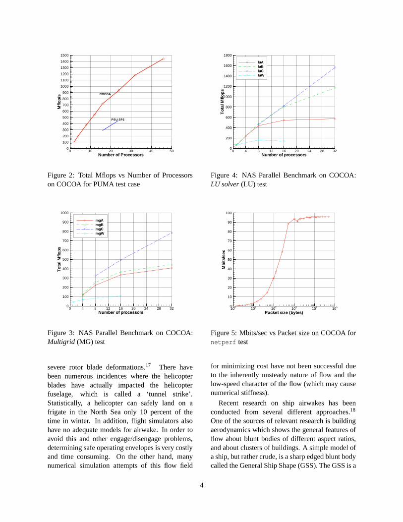
PUMA was chosen as one of the first benchmarks.Figure 2 shows the Mflops obtained from aninviscid run on a general ship shape (GSS)geometry on different number of processors usingPUMA. For this case, an unstructured tetrahedralgrid with 483;565 cells and 984;024 faces wasused and the run consumed 1:2 GB of RAM. Thebenchmark showed that COCOA was almost twiceas fast as the Penn State IBM SP (older 66 MHzRS/6000-370 nodes) for our applications.

Figure 5 shows the results obtained fromthe netperf test (done using: netperf -tUDPSTREAM -l 60 -H <target-machine>-- -s 65535 -m <packet-size> ). This isindicative of the communication speed betweenany two nodes. It is seen that almost 96% ofthe peak communication speed of 100 Mbit/sec isachieved between any two nodes for packet sizesabove 1;000 bytes.

A set of well-known parallel benchmarks relatedto CFD were also conducted on COCOA usingthe publicly availableNAS1 Parallel Benchmarks(NPB) suite v2.316 written in Fortran 77. Of theeight tests contained in the suite, five werekernelbenchmarks and the other three weresimulatedCFD application benchmarks. There were fourdifferent problem sizes for each test: Class “W”,“A”, “B” and “C”. While class “W” was theworkstation-size test (smallest), size “C” wassupercomputer-size test (largest). Figures 3 and4 show the performance of COCOA for each ofthe problem sizes for the LU solver and Multigridsolver tests, respectively.

Results

General Ship Shape (GSS)

The increasing use of helicopter in conjunctionwith ships poses many major problems. In thepresence of high winds and rough sea, excessiveship motions and turbulent, separated flow fromsharp-edged box-like ship super-structures makelanding a helicopter on ships a very hazardousoperation. The strong unsteady flows can cause

1NAS stands forNumerical Aerospace Simulationfacility,and is a part of NASA Ames Research Center

3

0 10 20 30 40 50Number of Processors

0

100

200

300

400

500

600

700

800

900

1000

1100

1200

1300

1400

1500M

flop

/s

PSU SP2

COCOA

Figure 2: Total Mflops vs Number of Processorson COCOA for PUMA test case

Number of processors

To

talM

flop

s

0 4 8 12 16 20 24 28 320

100

200

300

400

500

600

700

800

900

1000

mgAmgBmgCmgW

Figure 3: NAS Parallel Benchmark on COCOA:Multigrid (MG) test

severe rotor blade deformations.17 There havebeen numerous incidences where the helicopterblades have actually impacted the helicopterfuselage, which is called a ‘tunnel strike’.Statistically, a helicopter can safely land on afrigate in the North Sea only 10 percent of thetime in winter. In addition, flight simulators alsohave no adequate models for airwake. In order toavoid this and other engage/disengage problems,determining safe operating envelopes is very costlyand time consuming. On the other hand, manynumerical simulation attempts of this flow field

Number of processors

To

talM

flop

s

0 4 8 12 16 20 24 28 320

200

400

600

800

1000

1200

1400

1600

1800

luAluBluCluW

Figure 4: NAS Parallel Benchmark on COCOA:LU solver(LU) test

100 101 102 103 104 105

Packet size (bytes)

0

10

20

30

40

50

60

70

80

90

100

Mb

its/s

ec

Figure 5: Mbits/sec vs Packet size on COCOA fornetperf test

for minimizing cost have not been successful dueto the inherently unsteady nature of flow and thelow-speed character of the flow (which may causenumerical stiffness).

Recent research on ship airwakes has beenconducted from several different approaches.18

One of the sources of relevant research is buildingaerodynamics which shows the general features offlow about blunt bodies of different aspect ratios,and about clusters of buildings. A simple model ofa ship, but rather crude, is a sharp edged blunt bodycalled the General Ship Shape (GSS). The GSS is a

4

standard shape set forth by the United States Navyas a geometry to be used to compare flow solvers.The GSS represents a typical United States Navyfrigate with the area of interest being the flowfield on the aft deck. The aft deck primarily actsas a landing area for helicopter. The turbulent,separated flow caused by the ship structure canmake landing a helicopter extremely difficult. Thestrong unsteady flows can also cause severe bladedeformation during start up and shut down of ahelicopter. This GSS geometry unstructured gridand solution was completed in conjunction withthe Pennsylvania State University ship airwakestudies.2 More geometrically precise studies havebeen carried out in wind tunnels3, 4, 19and full scaletests have been conducted by the US Navy,5 whichprovide some important information on real shipairwakes. All these experimental tests are crucialfor validating numerical models. Wind tunnel testscan be quite costly, and the flow measurementson real Naval ships is very difficult and costly toobtain.

It would be very useful to have numericalmethods that could simulate ship airwakes. Therehave been other attempts at numerically simulatingship airwakes, e.g. a steady-state flow solver basedon the 3D multi-zone, thin-layer Navier-Stokes(TLNS) method20 and an unsteady, inviscid low-order method solver.21 No method to-date hasbeen entirely satisfactory for predicting these flowfields.

This was the first complex case which was usedto validate PUMA. The flow conditions were takento be M∞ = 0:065 and the yaw angleβ = 30Æ.Both inviscid and viscous (Re= 1:15�108) caseswere run.1 For the inviscid run, a structured gridwith 227;120 cells and 694;556 faces was usedand the run consumed 1:2 GB of memory. Forthe viscous run, an unstructured tetrahedral gridwith 483;565 cells and 984;024 faces was usedand the run consumed 1:1 GB of memory. Theconvergence history for the viscous run is shownin figure 6. It shows a plot of the relative residual2

against the number of iterations/timesteps. Thesurface velocity on the GSS geometry as computedby PUMA is shown in figure 30. Qualitative

2Ratio of the current residual to the initial residual

0 200 400 600 800Number of Iterations

10-4

10-3

10-2

10-1

100

Rel

ativ

eR

esid

ual

Figure 6: Convergence history for GSS viscous runfor 30Æ yaw case

comparisons were then made with the availableexperimental data.22 As seen in figures 8, 11 and14, which compare both the inviscid and viscoussolutions with the experiments, it is very clear thatPUMA gives very good solutions for this case. Theviscous solution is seen to be clearly better in theregion of flow separation.

The results, although extremely good, canbe improved by implementing the atmosphericboundary layer for the water surface, which hasbeen currently taken as a friction-less surface.

Apart from the above runs, 14 other inviscidcases were run using the unstructured grid. Thesecases were for yaw angles of 0Æ, 30Æ, 60Æ, 90Æ,120Æ, 150Æ and 180Æ, with two different flowspeeds of 40 and 50 knots, respectively. ThesurfaceU=U∞ contours for some of these cases canbe seen in figures 31, 32 and 33. These cases wererun to study the effect of various flow conditions onthe engage/disengage operations of the helicopterrotor. The region of interest for this study was therear deck of the ship (figure 34). More details onthis can be found in work by Keller and Smith.17

Viscous Sphere (Re= 1000)

A complete unsteady separated flow solution overa sphere in uniform flow has also been simulatedusing PUMA. Since flow over a sphere is aprototype example from the class of flows past

5

Figure 7: Oil flow pattern on front part of bridgedeck of GSS for 30Æ yaw case

Figure 8: Vector plot on front part of bridge deckof GSS for 30Æ yaw case (inviscid case)

Figure 9: Vector plot on front part of bridge deckof GSS for 30Æ yaw case (viscous case)

bluff bodies, and because extensive experimentaldata is available for it, this was considered an idealcase to use for the validation of PUMA.10

Figure 10: Oil flow pattern on middle part ofbridge deck of GSS for 30Æ yaw case

Figure 11: Vector plot on middle part of bridgedeck of GSS for 30Æ yaw case (inviscid case)

Figure 12: Vector plot on middle part of bridgedeck of GSS for 30Æ yaw case (viscous case)

The flow domain for this case was box shapedand is shown in figure 16. The grid extended for5 diameters in the front, the top and the bottom

6

Figure 13: Oil flow pattern on front deck of GSSfor 30Æ yaw case

Figure 14: Vector plot on front deck of GSS for30Æ yaw case (inviscid case)

Figure 15: Vector plot on front deck of GSS for30Æ yaw case (viscous case)

of the sphere, and 20 diameters behind. Theblockage ratio corresponding to these dimensionsis 0:65%. Since the boundary layer on the

sphere does not become turbulent until a Reynoldsnumber of the order of 300;000 is reached,estimates of the boundary layer thickness werederived from the laminar boundary layer solutionfor axisymmetric bodies.23 For this grid, 10 layersof prismatic cells were placed within the boundarylayer. The final viscous grid obtained consistedof 306;596 cells and 617;665 faces, and the runconsumed 600 MB of memory on 32 nodes ofCOCOA (running 2-stage Runge-Kutta). The flowconditions wereM∞ = 0:2 (U∞ = 68 m/s) andRe= 1000 based on the diameter. This case wasinitially run using SSOR to get a somewhat steadystate solution (with residual reduction of about2 orders in magnitude), and then switched overto a 2-stage time-accurate Runge-Kutta scheme.The time-accurate run commenced after 14;000iterations, but all data before iteration 50;000 wasdiscarded to avoid the transients. Therefore,t = 0corresponds to iteration 50;000. The convergencehistory for the run is shown in figure 17, and theCp and Mach contours along the planesX = 0 andZ = 0 are shown in figures 26 and 28. For thetime-accurate run, each timestep corresponds to∆t = 6:45911�10�7 sec= 2:197�10�5 diameterunits3. From the available experimental data, forRe= 1000, the Strouhal number is expected to bevery close to 0:2, thus giving a vortex sheddingperiod of approximatelyT = 0:15 sec= 5 units,for this simulation.

In spite of our running for just two cycles of thevortex shedding period (t = 10= 2T), the time-averagedCp results (figure 18) compared quitewell with the experimental data from Modi andAkutsu.24 The correlation between the surfaceCp values was almost perfect in the range 0Æ �

θ < 110Æ, but seemed to vary by approximatelya constant amount for the wake region (110Æ �

θ � 180Æ). Axial velocity data along the centerline trailing the center of the sphere are comparedto both the DNS simulation by Tomboulides,6

and the experimental data from Wu and Faeth25

in figures 22 and 23. The comparison is notperfect, but the results are encouraging. Thedifference can be attributed to the fact that the

3time required by the flow to convect one diameter in theflowfield

7

simulation described here ran for just two cyclesof vortex shedding (and 10 time units), unlike theDNS data from Tomboulides6 which was averagedover more than 20 shedding cycles. Due to theextremely small number of samples, our time-averaged results were very sensitive to the startingand ending points of the sampled data. Figure 19shows the time history plot of the non-dimensionalaxial velocity (v=U∞) of several points in the wakeof the sphere. Axial velocity profiles for differentplanes in the wake of the sphere are also shown infigure 20. The nature of the flow again matcheswith the experiments here, as reverse flow isnoticed only until about 1:8 diameters downstreamof the sphere (measuring from the center of thesphere). Figure 21 shows the variation of the lift(CL), drag (CD) and side force (CM) coefficientsover time of the simulation.

Figure 24 shows the iso-surface at which axialvelocity is 90% ofU∞ for the instantt = 9:34. Thisgives the approximate shape of the wake. Figure 25attempts to show the three-dimensional nature ofthe wake region for the same instant. Figure 27depicts the flow along the sliceX = 0 at differentinstants of time. Although the streamlines showndo not signify the actual unsteady streamlines, theydo give the general idea about the tendency of theflow. Streaklines are what are really needed to beshown, but they are very tedious and difficult toobtain. The figure clearly shows the alternatingnature of the vortex shedding fort =0 andt =2:75.However, the same observation cannot be made forthe latter two figures, maybe because the vortexshedding has not yet stabilized and thus cannot beconsidered periodic.

Other cases

Figure 35 shows the surface total velocity contoursfor a Landing Helicopter Aide (LHA) geometry.This case was run to study a specific spot on theLHA where a lot of problems have been seenin the event of a helicopter landing. The flowconditions were 25 knots (12:7 m/s) at 5Æ yaw.The inviscid grid consisted of 1;216;709 cells and2;460;303 faces and the run consumed 2:3 GB ofRAM. The initial 2;000 timesteps were traversedusing SSOR and the remaining timesteps using

-10

-5

0

5

10

Z

-10

-5

0

5

10

X

-10

0

10

20

30

40

Y

X Y

Z

Figure 16: Domain for the viscous sphere grid

0 100000 200000 300000 400000 500000Number of Iterations

10-3

10-2

10-1

100

Rel

ativ

eR

esid

ual

Figure 17: Convergence history for viscous sphererun (M∞ = 0:2, Re= 1000)

the less expensive 2-stage Jameson-style Runge-Kutta scheme. The entire run took 39 hours on 32processors of COCOA.

Figure 29 shows surface Mach contours for anApache helicopter geometry. The flow conditionswereU∞ = 114 knots. The inviscid grid consistedof 555;772 cells and 1;125;596 faces and the runconsumed 1:9 GB of RAM.

Conclusions

A complete, fast and efficient unstructured gridbased flow solution around several complex

8

θ

Cp

0 15 30 45 60 75 90 105 120 135 150 165 180

-0.2

-0.1

0.0

0.1

0.2

0.3

0.4

0.5

0.6

0.7

0.8

0.9

1.0

PUMA (upper surf)PUMA (lower surf)Experiment

Figure 18: Time averaged plot forCp vsθ for uppersurface compared with experiments,24 for viscoussphere run (M∞ = 0:2, Re= 1000) [Note: Here,Cp

is defined as(Pθ�P60Æ)=(P0Æ�P60Æ)]

t

v/U

inf

0 1 2 3 4 5 6 7 8 9 10-1.00

-0.80

-0.60

-0.40

-0.20

0.00

0.20

0.40

0.60

0.80

1.00

0.55D1.00D1.50D2.00D5.00D

Figure 19: Time history depicting axial velocityfor points at fixed distances behind the center ofthe sphere along they-axis

geometries has been demonstrated. The objectiveto achieve this at a very affordable cost usinginexpensive departmental level supercomputingresources like COCOA, has been fulfilled.

The flow solver PUMA has been verifiedwith experimental data from inviscid and viscoussolutions around the GSS geometry. Althoughthe experimental data was qualitative in nature,the excellent correlation between the two for

U/U inf

y

-0.8 -0.6 -0.4 -0.2 0.0 0.2 0.4 0.6 0.8 1.0 1.2-4

-3

-2

-1

0

1

2

3

4

0.5 D1.0 D1.5 D2.0 D5.0 D

Sphere

Figure 20: Instantaneous velocity profile (t = 8:79)showing wake region for viscous sphere run (M∞ =

0:2, Re= 1000)

t

CL,C

D,C

M

0 2 4 6 8 10-0.1

0.0

0.1

0.2

0.3

0.4

0.5

0.6

CL

CD

CM

Figure 21: Variation of totalCl , Cd and Cm

coefficients with time for viscous sphere run(M∞ = 0:2, Re= 1000)

such a complex flow was extremely encouraging.Both the inviscid and viscous solutions comparedvery well, with the viscous solution being betterin the region of flow separation. Recentwork by Schweitzer9 has also compared inviscidsolutions from PUMA around the ROBIN bodywith experiments, and the outcome was veryfavorable. Several other large problems forflow around different ship configurations (LHA,aircraft carrier CVN-75) and helicopter fuselages

9

x/D

u/U

0 1 2 3 4 5 6 7 8 9 10

-0.2

-0.1

0.0

0.1

0.2

0.3

0.4

0.5

0.6

0.7

0.8

0.9

1.0

PUMADNSExperiment

Time averaged data for Re=1000

Figure 22: Time averaged axial velocity plot(v=U∞) for viscous sphere run (M∞ = 0:2, Re=1000)

x/D

u’/U

0 1 2 3 4 5 6 7 8 9 100.00

0.05

0.10

0.15

0.20

0.25

PUMADNSExperiment

RMS data for Re=1000

Figure 23: Time averaged RMS velocity plot(v0=U∞) for viscous sphere run (M∞ = 0:2, Re=1000)

(AH-64 Apache, Boeing generic fuselage) havebeen run, but lack of any experimental data hasprevented the measure of PUMA’s success forthese cases. Viscous, unsteady runs forRe=1000 around a finite cylinder and sphere have alsobeen conducted. For the sphere case, in spiteof our running for just two cycles of the vortexshedding period, the time-averagedCp resultscompared quite well with the experimental data.The correlation between the surfaceCp values

Figure 24: Iso-surface at which axial velocity is90% ofU∞ (t = 9:34)

was almost perfect in the range 0Æ � θ < 110Æ,but seemed to vary by approximately a constantamount for the wake region (110Æ � θ � 180Æ).The code also was able to predict the trends inthe wake axial velocity, although there were somediscrepancies. This can be attributed to the factthat the simulation described here ran for just twocycles of vortex shedding (10 time units), whichmade the data statistically stiff, as compared to theDNS data which was averaged over more than 20cycles. Based on the validation and the experiencefrom the above runs, PUMA is seen to be a verygood starting point for modeling such complexunsteady separated flows. We plan to run LESsimulations in the near future.

COCOA was found to be extremely suitablefor our numerical simulations. One of the realbenefits of inexpensive machines is that they donot have to be shared with hundreds of otherusers, and we do not have to wait days in aqueueing system. We quite often have to waitseveral days at a supercomputer center just to use16 processors. Also, while it is quite difficult toget 50;000 CPU hours at a supercomputer center,our Beowulf cluster gives us more than 400;000CPU hours per year. COCOA was also foundto have good scalability with most of the MPIapplications used. Although Beowulf clusters havevery high latency as compared to conventionalsupercomputers, this did not affect our applications

10

Figure 25: Mach contour slices every 2 diametersin the wake region for the viscous sphere run(M∞ = 0:2, Re= 1000)

as most of our codes had only a few largemessages being communicated at every timestep.For those codes that have high communication tocomputation ratios, COCOA was not found to bean ideal platform because of the high latency. Withseveral more enhancements planned for COCOAin the near future, including the addition ofseveral more nodes and increasing the networkingbandwidth by addition of more fast-ethernet cardsto every node, the performance is expected toincrease. Faster interconnect networks could alsobe used, such as Myrinet, Gigabit, or ATM; butthese would increase the cost of the system byapproximately 50%.

References

[1] Long, L. N., Liu, J., and Modi, A., “HigherOrder Accurate Solutions of Ship AirwakeFlow Fields Using Parallel Computers,”RTOAVT Symposium on Fluid Dynamics Prob-lems of Vehicles Operating near or in the Air-Sea Interface, Oct. 1998.

[2] Liu, J. and Long, L. N., “Higher Order Ac-curate Ship Airwake Predictions for the Heli-copter/Ship Interface Problem,”54th AnnualAmerican Helicopter Society Forum, 1998.

Figure 26: Cp contours for viscous sphere run(M∞ = 0:2, Re= 1000)

[3] Rhoades, M. M. and Healey, J. V., “FlightDeck Aerodynamics of a Non-aviation Ship,”Journal of Aircraft, Vol. 29, No. 4, 1992,pp. 619–626.

[4] Hurst, D. W. and Newman, S., “Wind Tun-nel Measurements of Ship Induced Turbu-lence and the Prediction of Helicopter Ro-tor Blade Response,”Vertica, Vol. 12, No. 3,1988, pp. 267–278.

[5] Williams, S. and Long, K. R., “Dynamic In-terface Testing and the Pilots Rating Scale,”The 53rd AHS Forum, Apr. 1997.

[6] Tomboulides, A. G.,Direct and Large-EddySimulation of Wake Flows: Flow Past aSphere, PhD Dissertation, Princeton Univer-sity, Jun. 1993.

[7] Bruner, C. W. S.,Parallelization of the Eu-ler equations on unstructured grids, PhD Dis-sertation, Virginia Polytechnic Institute andState University, May 1996.

[8] Pirzadeh, S., “Progress Toward a User-Oriented Unstructured Viscous Grid Gener-ator,” AIAA Paper 96-0031, Jan. 1996.

[9] Schweitzer, S.,Computational Simulationof Flow around Helicopter Fuselages, M.S.

11

Figure 27: Mach contours and streamlines (att =0:0;2:75) for viscous sphere run (M∞ = 0:2, Re=1000)

Thesis, The Pennsylvania State University,Jan. 1999.

[10] Modi, A., Unsteady Separated Flow Simula-tions using a Cluster of Workstations, M.S.Thesis, The Pennsylvania State University,May 1999.

[11] Modi, A., “COst effective COmputing Ar-ray,” http://cocoa.ihpca.psu.edu, 1998.

[12] Kantor, A., Long, L. N., and Micci, M. M.,“Molecular Dynamics Simulation of Dissoci-ation Kinetics,”AIAA Paper 2000-0213, Jan.2000.

Figure 28: Mach contours for viscous sphere run(M∞ = 0:2, Re= 1000)

Figure 29: Surface Mach contours for Apachehelicopter geometry (U∞ = 114 knots)

[13] Long, L. N. and Brentner, K. A., “SelfScheduling Parallel Version of Wopwop,”AIAA Paper 2000-0346, Jan. 2000.

[14] Hall, C. M. and Long, L. N., “Higher OrderAccurate Methods for Vortex Flow Simlua-tions,” AHS Forum, Montreal, Canada, May1999.

[15] Morris, P. J., L. L. N. and Scheidegger, T.,“Parallel Computations of High Speed JetNoise,”AIAA Paper 99-1873, May 1999.

12

Figure 30: SurfaceU=U∞ contours for GSSgeometry for 30Æ yaw case

Figure 31: SurfaceU=U∞ contours for GSSgeometry for flow speeds of 40 knots and yawangle of 30Æ

[16] Woo, A., “NAS Parallel Benchmarks,”http://science.nas.nasa.gov/Software/NPB/,1997.

[17] Keller, J. and Smith, E., “Analysis and Con-trol of the Transient Shipboard EngagementBehavior of Rotor Systems,”Proceedings ofthe 55th Annual National Forum of the Amer-ican Helicopter Society (Montreal, Canada),May 1999.

[18] Healey, J. V., “The Prospects for Simulating

Figure 32: SurfaceU=U∞ contours for GSSgeometry for flow speeds of 40 knots and yawangle of 90Æ

Figure 33: SurfaceU=U∞ contours for GSSgeometry for flow speeds of 40 knots and yawangle of 150Æ

the Helicopter/Ship Interface,”Naval Engi-neers Journal, Mar. 1987, pp. 45–63.

[19] Healey, J. V., “Establishing a Database forFlight in the Wake of Structures,”Journal ofAircraft, Vol. 29, No. 4, 1992, pp. 559–564.

[20] Tai, T. C. and Cario, D., “Simulation ofDD-963 Ship Airwake by Navier-StokesMethod,”AIAA Paper 93-3002, 1993.

13

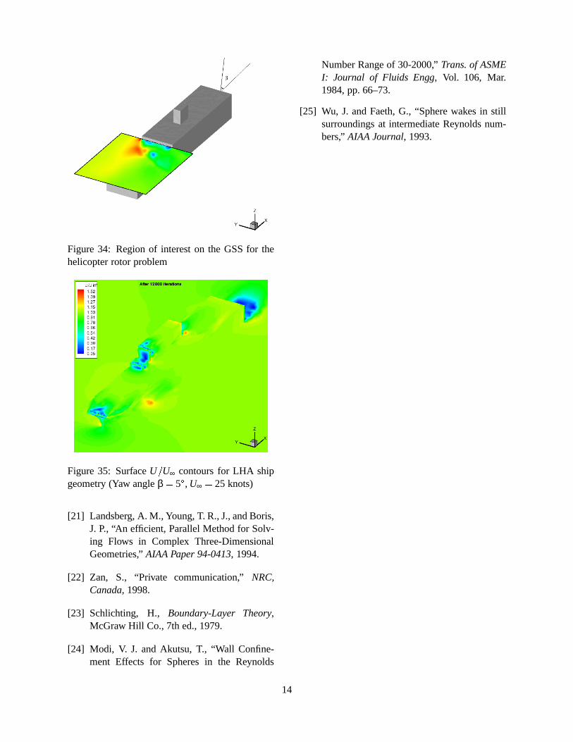
Figure 34: Region of interest on the GSS for thehelicopter rotor problem

Figure 35: SurfaceU=U∞ contours for LHA shipgeometry (Yaw angleβ = 5Æ, U∞ = 25 knots)

[21] Landsberg, A. M., Young, T. R., J., and Boris,J. P., “An efficient, Parallel Method for Solv-ing Flows in Complex Three-DimensionalGeometries,”AIAA Paper 94-0413, 1994.

[22] Zan, S., “Private communication,”NRC,Canada, 1998.

[23] Schlichting, H., Boundary-Layer Theory,McGraw Hill Co., 7th ed., 1979.

[24] Modi, V. J. and Akutsu, T., “Wall Confine-ment Effects for Spheres in the Reynolds

Number Range of 30-2000,”Trans. of ASMEI: Journal of Fluids Engg, Vol. 106, Mar.1984, pp. 66–73.

[25] Wu, J. and Faeth, G., “Sphere wakes in stillsurroundings at intermediate Reynolds num-bers,”AIAA Journal, 1993.

14