aimms tutorial beginners

AIMMSA One-Hour Tutorial

for BeginnersMarch 2010

Paragon Decision Technology

Johannes BisschopKoos Heerink

Copyright c© 1993–2010 by Paragon Decision Technology B.V. All rights reserved.

Paragon Decision Technology B.V.Schipholweg 12034 LS HaarlemThe NetherlandsTel.: +31 23 5511512Fax: +31 23 5511517

Paragon Decision Technology Inc.500 108th Avenue NESte. # 1085Bellevue, WA 98004USATel.: +1 425 458 4024Fax: +1 425 458 4025

Paragon Decision Technology Pte.Ltd.80 Raffles PlaceUOB Plaza 1, Level 36-01Singapore 048624Tel.: +65 9640 4182

Email: [email protected]: www.aimms.com

ISBN xx–xxxxxx–x–x

Aimms is a registered trademark of Paragon Decision Technology B.V. IBM ILOG CPLEX and sc CPLEX isa registered trademark of IBM Corporation. GUROBI is a registered trademark of Gurobi Optimization,Inc. KNITRO is a registered trademark of Ziena Optimization, Inc. XPRESS-MP is a registered trademarkof FICO Fair Isaac Corporation. Mosek is a registered trademark of Mosek ApS. Windows and Excel areregistered trademarks of Microsoft Corporation. TEX, LATEX, and AMS-LATEX are trademarks of the AmericanMathematical Society. Lucida is a registered trademark of Bigelow & Holmes Inc. Acrobat is a registeredtrademark of Adobe Systems Inc. Other brands and their products are trademarks of their respectiveholders.

Information in this document is subject to change without notice and does not represent a commitment onthe part of Paragon Decision Technology B.V. The software described in this document is furnished undera license agreement and may only be used and copied in accordance with the terms of the agreement. Thedocumentation may not, in whole or in part, be copied, photocopied, reproduced, translated, or reduced toany electronic medium or machine-readable form without prior consent, in writing, from Paragon DecisionTechnology B.V.

Paragon Decision Technology B.V. makes no representation or warranty with respect to the adequacyof this documentation or the programs which it describes for any particular purpose or with respectto its adequacy to produce any particular result. In no event shall Paragon Decision Technology B.V.,its employees, its contractors or the authors of this documentation be liable for special, direct, indirector consequential damages, losses, costs, charges, claims, demands, or claims for lost profits, fees orexpenses of any nature or kind.

In addition to the foregoing, users should recognize that all complex software systems and their doc-umentation contain errors and omissions. The authors, Paragon Decision Technology B.V. and its em-ployees, and its contractors shall not be responsible under any circumstances for providing informationor corrections to errors and omissions discovered at any time in this book or the software it describes,whether or not they are aware of the errors or omissions. The authors, Paragon Decision TechnologyB.V. and its employees, and its contractors do not recommend the use of the software described in thisbook for applications in which errors or omissions could threaten life, injury or significant loss.

This documentation was typeset by Paragon Decision Technology B.V. using LATEX and the Lucida fontfamily.

http://www.aimms.com

Contents

Contents iii

Common Aimms Shortcut Keys iv

1 Introduction 1

2 What to Expect 32.1 Scope of one-hour tutorial . . . . . . . . . . . . . . . . . . . . . . 32.2 Problem description and model statement . . . . . . . . . . . . 32.3 A preview of your output . . . . . . . . . . . . . . . . . . . . . . 6

3 Building the Model 73.1 Starting a new project . . . . . . . . . . . . . . . . . . . . . . . . 73.2 The Model Explorer . . . . . . . . . . . . . . . . . . . . . . . . . . 83.3 Entering sets and indices . . . . . . . . . . . . . . . . . . . . . . . 93.4 Entering parameters and variables . . . . . . . . . . . . . . . . . 103.5 Entering constraints and the mathematical program . . . . . 133.6 Viewing the identifiers . . . . . . . . . . . . . . . . . . . . . . . . 15

4 Entering and Saving the Data 214.1 Entering set data . . . . . . . . . . . . . . . . . . . . . . . . . . . . 214.2 Entering parameter data . . . . . . . . . . . . . . . . . . . . . . . 224.3 Saving your data . . . . . . . . . . . . . . . . . . . . . . . . . . . . 24

5 Solving the Model 275.1 Computing the solution . . . . . . . . . . . . . . . . . . . . . . . 27

6 Building a 06.1 Creating a new page . . . . . . . . . . . . . . . . . . . . . . . . . . 306.2 Presenting the input data . . . . . . . . . . . . . . . . . . . . . . 306.3 Presenting the output data . . . . . . . . . . . . . . . . . . . . . 336.4 Finishing the page . . . . . . . . . . . . . . . . . . . . . . . . . . . 35

7 Performing a What-If Run 407.1 Modifying input data . . . . . . . . . . . . . . . . . . . . . . . . . 40

Common Aimms Shortcut Keys 42

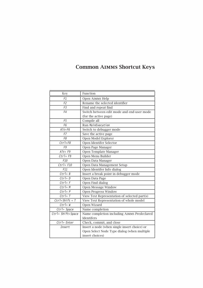
Common Aimms Shortcut Keys

Key Function

F1 Open Aimms Help

F2 Rename the selected identifier

F3 Find and repeat find

F4 Switch between edit mode and end-user mode(for the active page)

F5 Compile all

F6 Run MainExecution

Alt+F6 Switch to debugger mode

F7 Save the active page

F8 Open Model Explorer

Ctrl+F8 Open Identifer Selector

F9 Open Page Manager

Alt+ F9 Open Template Manager

Ctrl+ F9 Open Menu Builder

F10 Open Data Manager

Ctrl+ F10 Open Data Management Setup

F11 Open Identifer Info dialog

Ctrl+ B Insert a break point in debugger mode

Ctrl+ D Open Data Page

Ctrl+ F Open Find dialog

Ctrl+ M Open Message Window

Ctrl+ P Open Progress Window

Ctrl+ T View Text Representation of selected part(s)

Ctrl+Shift + T View Text Representation of whole model

Ctrl+ W Open Wizard

Ctrl+ Space Name completion

Ctrl+ Shift+Space Name completion including Aimms PredeclaredIdentifers

Ctrl+ Enter Check, commit, and close

Insert Insert a node (when single insert choice) orOpen Select Node Type dialog (when multipleinsert choices)

Chapter 1

Introduction

Ways to learnAimms . . .

There are several ways in which you can learn the Aimms language and get a ba-sic understanding of its underlying development environment. The followingopportunities are immediately available, and are part of the Aimms installation.

� There are two tutorials on Aimms to provide you with some initial work-ing knowledge of the system and its language. One tutorial is intendedfor beginners, while the other is aimed at professional users of Aimms.

� There is a model library with a variety of examples to illustrate simpleand advanced applications together with particular aspects of both thelanguage and the graphical user interface.

� There are three reference books on Aimms, which are available in PDF for-mat and in hard copy form. They are The User’s Guide to introduce youto Aimms and its development environment, The Language Reference todescribe the modeling language in detail, and Optimization Modeling toenable you to become familiar with building models.

. . . for beginnersAs a beginner into optimization modeling languages, you may not have muchtime for learning yet another tool in order to finish some project or home-work requirements. In this case, concentrate your efforts on this tutorial. Af-ter completing this tutorial, you should be able to use the system to buildyour own simple models, and to enter your own small data sets for subse-quent viewing. The book on Optimization Modeling may teach you some usefultricks, and will show you different (mostly non-trivial) examples of optimiza-tion models. Besides English, the tutorial for beginners is also available inSpanish, Hungarian, German and French, which can be found on our web site:http://www.aimms.com/downloads/tutorials/tutorial-for-beginners.

. . . forprofessionals

As a professional in the field of optimization modeling you are looking for atool that simplifies your work and minimizes the time needed for model con-struction and model maintenance. In this situation, you cannot get around thefact that you will need to initially make a substantial time investment to get toknow several of the advanced features that will subsequently support you inyour role as a professional application builder. Depending on your skills, expe-rience, and learning habits you should determine your own individual learningpath. Along this path you are advised to work through the extensive tutorial

http://www.aimms.com/downloads/tutorials/tutorial-for-beginners

Chapter 1. Introduction 2

especially designed for professionals. This tutorial for professionals providesa good start, and should create excitement about the possibilities of Aimms.Individual examples in the library, plus selected portions of the three books,will subsequently offer you additional ideas on how to use Aimms effectivelywhile building your own advanced applications.

Tutorials aredifferent inscope

The one-hour tutorial for beginners is designed as the bare minimum neededto build simple models using the Aimms Model Explorer. Data values are en-tered by hand using data pages, and the student can build a page with objectsto view and modify the data. The extensive tutorial for professionals is an elab-orate tour of Aimms covering a range of advanced language features plus anintroduction to all the building tools. Especially of interest will be the modelingof time using the concepts of horizon and calendar, the use of quantities andunits, the link to a database, the connection to an external DLL, and advancedreporting facilities. Even then, some topics such as efficiency considerations(execution efficiency, matrix manipulation routines) and the Aimms API willremain untouched.

Chapter 2

What to Expect

This chapterIn this chapter you will find a brief overview of the tasks to be performed, acompact statement of the underlying model to be built, and a glimpse of theoutput you will produce.

2.1 Scope of one-hour tutorial

Summarizingyour work

Once you have read the short problem description and the associated mathe-matical model statement, you will be asked to complete a series of tasks thatmake up this one-hour tutorial, namely:

� create a new project in Aimms,� enter all identifier declarations,� enter the data manually,� save your data in a case,� build a small procedure,� build a single page with

– header text,– a standard table and two bar charts with input data,– a composite table and a stacked bar chart with output data,– a button to execute the procedure, and– a scalar object with the optimal value,

� perform a what-if run.

2.2 Problem description and model statement

Problemdescription

Truckloads of beer are to be shipped from two plants to five customers dur-ing a particular period of time. Both the available supply at each plant andthe required demand by each customer (measured in terms of truckloads) areknown. The cost associated with moving one truck load from a plant to acustomer is also provided. The objective is to make a least-cost plan for mov-ing the beer such that the demand is met and shipments do not exceed theavailable supply from each brewery.

Chapter 2. What to Expect 4

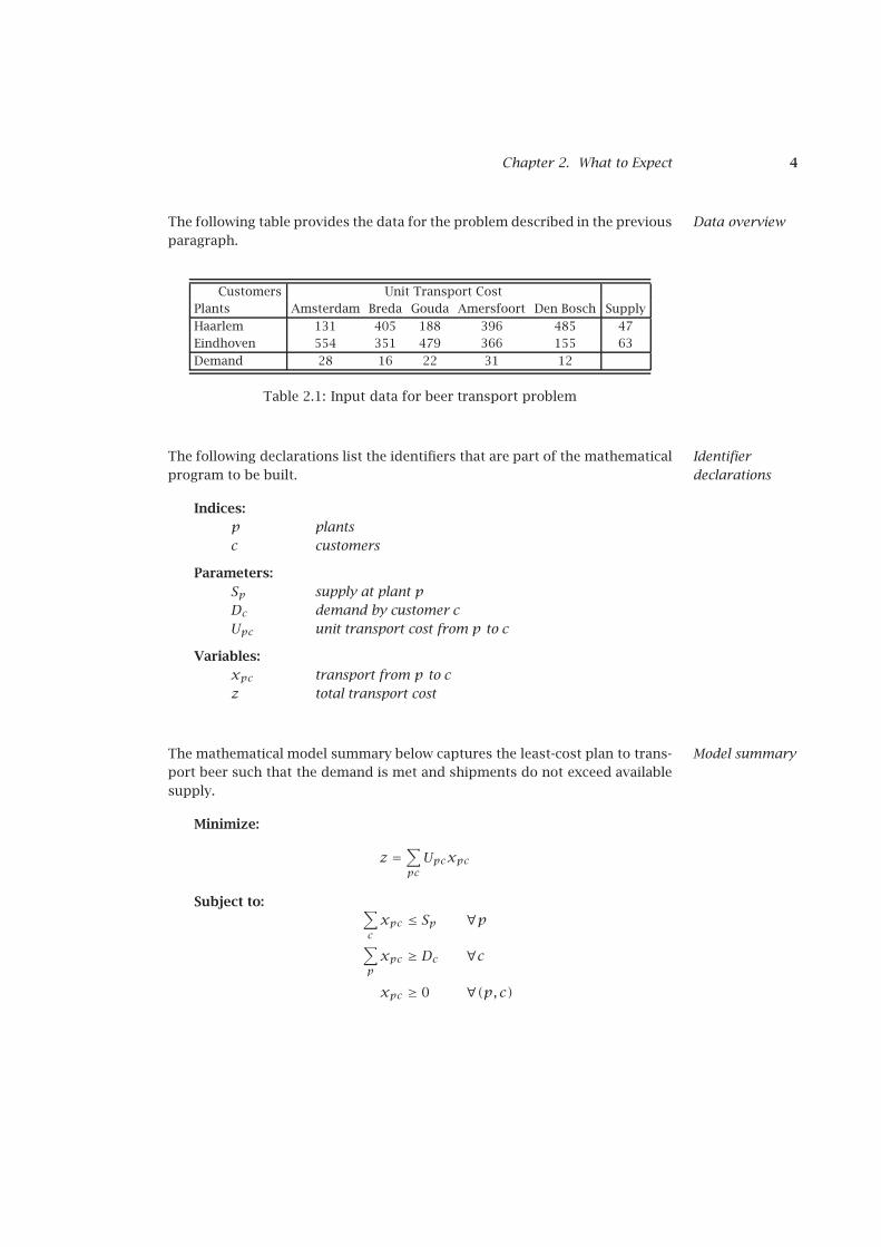
Data overviewThe following table provides the data for the problem described in the previousparagraph.

Customers Unit Transport CostPlants Amsterdam Breda Gouda Amersfoort Den Bosch Supply

Haarlem 131 405 188 396 485 47Eindhoven 554 351 479 366 155 63

Demand 28 16 22 31 12

Table 2.1: Input data for beer transport problem

Identifierdeclarations

The following declarations list the identifiers that are part of the mathematicalprogram to be built.

Indices:p plantsc customers

Parameters:Sp supply at plant pDc demand by customer cUpc unit transport cost from p to c

Variables:xpc transport from p to cz total transport cost

Model summaryThe mathematical model summary below captures the least-cost plan to trans-port beer such that the demand is met and shipments do not exceed availablesupply.

Minimize:

z =∑

pcUpcxpc

Subject to: ∑

cxpc ≤ Sp ∀p

∑

pxpc ≥ Dc ∀c

xpc ≥ 0 ∀(p, c)


AmsterdamHaarlem

Gouda

Amersfoort

Breda

Den Bosch

Eindhoven

Figure 2.1: The Netherlands

Using explicitnames

Even though the above notation with one-letter symbols is typical of smallmathematical optimization models, it will not be used to represent the modelin Aimms. Instead, explicit names will be used throughout to avoid any un-necessary translation symbols. The number of symbols needed to describepractical applications is generally large, and a clear naming convention sup-ports the understanding and maintenance of large models.


2.3 A preview of your output

A single pageFigure 2.2 is a page that contains both input and output data associated withthe beer transport model. In Chapter 6 you will be asked to construct this pageusing the point-and-click facilities available in Aimms.

Figure 2.2: An input-output page

Chapter 3

Building the Model

3.1 Starting a new project

Starting AimmsAssuming that Aimms 3 has already been installed on your machine. If thereis an Aimms 3 shortcut on your desktop, double click it to start Aimms 3,otherwise execute the following sequence of actions to start Aimms:

� press the Start button on the taskbar,� go to the Programs submenu, and� select and click on the Aimms icon to start Aimms.

Specifying aproject name

Next, you will see the Aimms splash screen. Once Aimms has started, the splashscreen will disappear and the Aimms window will open. Should you encounterthe Aimms Tip of the Day dialog box, close it, because it is not relevant to youat this point.

Creating a newproject fromwithin Aimms

Press the New Project button , which is located in the leftmost positionon the Aimms toolbar. The dialog box shown in Figure 3.1 will then appear,requiring you to take the following actions:

� specify ‘Beer Transport’ as the project name, and� press the wizard button to select the folder for your Aimms projects

if the default folder‘...\My Documents\My AIMMS Projects\Beer Transport’is not desired,and

� press the OK button.

Chapter 3. Building the Model 8

Figure 3.1: The New Project wizard

Next, the Aimms Model Explorer and the Aimms Page Manager will be auto-matically opened. We will look at the Aimms Model Explorer first.

3.2 The Model Explorer

Initial modeltree

When opened for the first time, the Aimms Model Explorer will display theinitial model tree shown in Figure 3.2. In this initial model tree you will see

� a single declaration section, where you can store the declarations used inyour model,

� the predefined procedure MainInitialization, which is not relevant forthis tutorial,

� the predefined procedure MainExecution, where you will put the executionstatement necessary to solve the mathematical program, and

� the predefined procedure MainTermination, which is again not relevantfor this tutorial.

Figure 3.2: The initial model tree


3.3 Entering sets and indices

Opening thedeclarationsection

The declaration of model identifiers requires you to first ‘open’ the declarationsection. You can do this either by clicking the icon or by double-clickingon the scroll icon . Note that double-clicking on the name of the declarationsection instead of on its icon will open the attribute form of the declarationsection and will therefore, at this point, not lead to the desired result. Afteropening the declaration section the standard identifier buttonson the toolbar will be enabled.

Creating the set‘Plants’

To create a set of plants you should take the following actions:

� press the Set button to create a new set identifier in the model tree,� specify ‘Plants’ as the name of the set, and� press the Enter key to register the name.

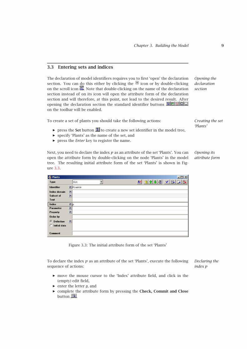
Opening itsattribute form

Next, you need to declare the index p as an attribute of the set ‘Plants’. You canopen the attribute form by double-clicking on the node ‘Plants’ in the modeltree. The resulting initial attribute form of the set ‘Plants’ is shown in Fig-ure 3.3.

Figure 3.3: The initial attribute form of the set ‘Plants’

Declaring theindex p

To declare the index p as an attribute of the set ‘Plants’, execute the followingsequence of actions:

� move the mouse cursor to the ‘Index’ attribute field, and click in the(empty) edit field,

� enter the letter p, and� complete the attribute form by pressing the Check, Commit and Close

button .


Creating the set‘Customers’

Next, create the set ‘Customers’ with associated index c in exactly the sameway as you created the set ’Plants’ with index domain p. Figure 3.4 containsthe resulting model tree.

Figure 3.4: An intermediate model tree

Saving yourchanges

The asterisk on the left of the project name indicates that additions to yourproject have not yet been saved to disk. To save your work, please press theSave Project button on the toolbar.

3.4 Entering parameters and variables

Domainspecification

In this section you will declare the parameters and variables that are neededin your model. The sets ‘Plants’ and ‘Customers’ and their associated indiceswill be used to specify the index domain for the parameters and variables.

Creating theparameter‘Supply’

The declaration of a parameter is similar to the declaration of a set. To enterthe parameter ‘Supply(p)’, you should execute the following actions:

� press the parameter button on the toolbar to create a new parameterin the model tree,

� specify ‘Supply(p)’ as the name of the parameter, and� press the Enter key to register the name.

Note that parentheses are used to add the index domain p to the identifier‘Supply’.

Creating theparameter‘Demand’

The parameter ’Demand(c)’ can be added in the same way. Should you make amistake in entering the information, then you can always re-edit a name fieldby a single mouse click within the field.


Creating theparameter‘UnitTransport-Cost’

The last model parameter ‘UnitTransportCost’ is a two-dimensional parameterwith index domain (p, c). After entering ‘UnitTransportCost(p,c)’, the resultingmodel tree should be the same as in Figure 3.5.

Figure 3.5: An intermediate model tree

Creating thevariable‘Transport’

Declaring a variable is similar to declaring a parameter.

� press the variable button on the toolbar to create a new variable inthe model tree,

� specify ‘Transport(p,c)’ as the name of the variable, and� press the Enter key to register the variable.

Specifyingrange attribute

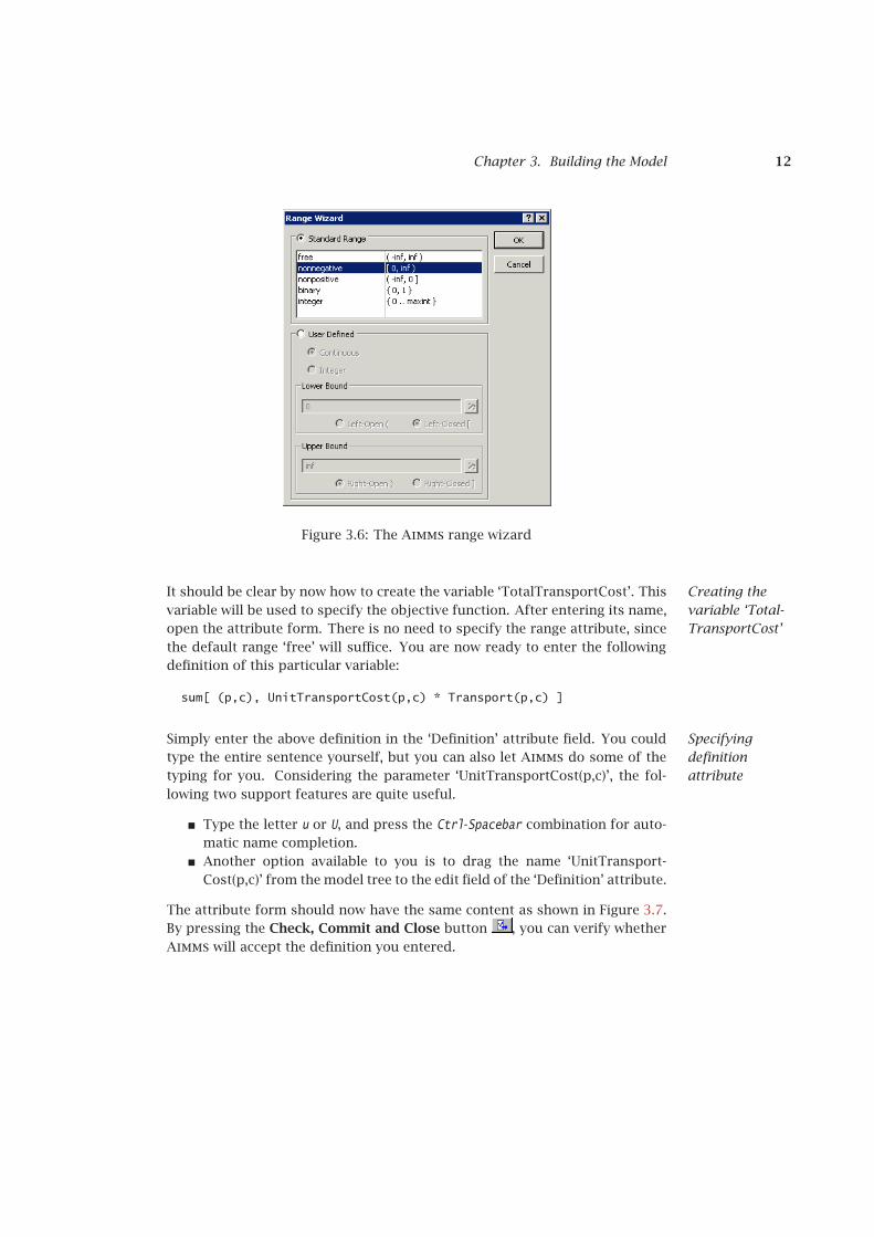
After opening the attribute form of the variable by double-clicking on the node‘Transport’ in the model tree, press the wizard button in front of the ‘Range’attribute field. The resulting dialog box provides the opportunity to specifythe range of values that the variable ‘Transport’ is allowed to take. In thiscase, select the ‘Standard Range’, then select ‘nonnegative’, and finally pressthe OK button (see Figure 3.6).


Figure 3.6: The Aimms range wizard

Creating thevariable ‘Total-TransportCost’

It should be clear by now how to create the variable ‘TotalTransportCost’. Thisvariable will be used to specify the objective function. After entering its name,open the attribute form. There is no need to specify the range attribute, sincethe default range ‘free’ will suffice. You are now ready to enter the followingdefinition of this particular variable:

sum[ (p,c), UnitTransportCost(p,c) * Transport(p,c) ]

Specifyingdefinitionattribute

Simply enter the above definition in the ‘Definition’ attribute field. You couldtype the entire sentence yourself, but you can also let Aimms do some of thetyping for you. Considering the parameter ‘UnitTransportCost(p,c)’, the fol-lowing two support features are quite useful.

� Type the letter u or U, and press the Ctrl-Spacebar combination for auto-matic name completion.

� Another option available to you is to drag the name ‘UnitTransport-Cost(p,c)’ from the model tree to the edit field of the ‘Definition’ attribute.

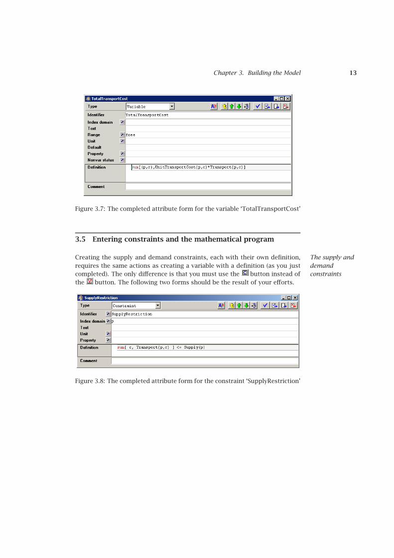
The attribute form should now have the same content as shown in Figure 3.7.By pressing the Check, Commit and Close button , you can verify whetherAimms will accept the definition you entered.


Figure 3.7: The completed attribute form for the variable ‘TotalTransportCost’

3.5 Entering constraints and the mathematical program

The supply anddemandconstraints

Creating the supply and demand constraints, each with their own definition,requires the same actions as creating a variable with a definition (as you justcompleted). The only difference is that you must use the button instead ofthe button. The following two forms should be the result of your efforts.

Figure 3.8: The completed attribute form for the constraint ‘SupplyRestriction’


Figure 3.9: The completed attribute form for the constraint ‘DemandRequire-ment’

Creating themathematicalprogram

A mathematical program, unlike sets, parameters, variables and constraints,does not have a special button on the toolbar. By using the identifier button

, you obtain access to all the other types of Aimms identifiers. After pressingthis button, select the ‘Mathematical Program’ entry alongside the icon,press the OK button, and enter ‘LeastCostTransportPlan’ as the name of themathematical program.

Specifying itsattributes

The complete the attribute form of the mathematical program as illustrated inFigure 3.10. Among the attributes, AIMMS has automatically filled Direction,Constraints, Variables and Type attributes with default values and there isno need to change them for this project. You only need to fill the Objectiveattribute.

Figure 3.10: The completed attribute form of the mathematical program

Selecting theobjective

The Objective attribute wizard requires you to select a scalar variable. In theidentifier selection wizard (see Figure 3.11), simply select the scalar variable‘TotalTransportCost’, and press the Finish button.


Figure 3.11: The identifier selection wizard

3.6 Viewing the identifiers

Checking yourmodel

You have now entered and declared all model identifiers. The resulting modeltree is shown in Figure 3.12. By pressing the F5 key you can instantly checkthe validity of your model. You will only receive a message in the event of anerror. Once the validity of your model has been verified, you should save yourwork by pressing the Save Project button .


Figure 3.12: The final model tree

Even though the Model Explorer is a convenient medium with which to buildand inspect your model, AIMMS provides two other ways to view your model.

View text modelIf you would like to see a text(ASCII) representation of the model, you can dothe following:

� select node(s) in Aimms Model Explorer,� go to the View - Text Representation menu and execute the Selected

Part(s) command(see Figure 3.13).


Figure 3.13: View text model

The text model provides a simple overview of selected identifiers. For instance,Figure 3.14 shows the text model when the root node Main Beer Transport isselected.


Figure 3.14: text model

Identifieroverviews

Another way to inspect the model is by Aimms Identifier Selector. This allowsyou to view several identifiers with similar properties at the same time. In thistutorial you will encounter one such example of a predefined view, namely allidentifiers with a definition (see Figure 3.15). Aimms allows you to make yourown views as you desire.

Figure 3.15: View window with identifier definitions


Creating a viewYou can create a view window by executing the following steps:

� press the Identifier Selector button on the toolbar,� select the ‘Identifiers with Definition’ node, and� use the right mouse and select the Open With. . . command from the

popup menu (see Figure 3.16).

Figure 3.16: Identifier Selector window

For the selected identifiers the view can be constructed as follows:

� select the ‘Domain - Definition’ entry from the View Manager window(see Figure 3.17), and

� press the Open button to obtain the overall view.


Figure 3.17: View Manager window

Chapter 4

Entering and Saving the Data

4.1 Entering set data

Manual dataentry

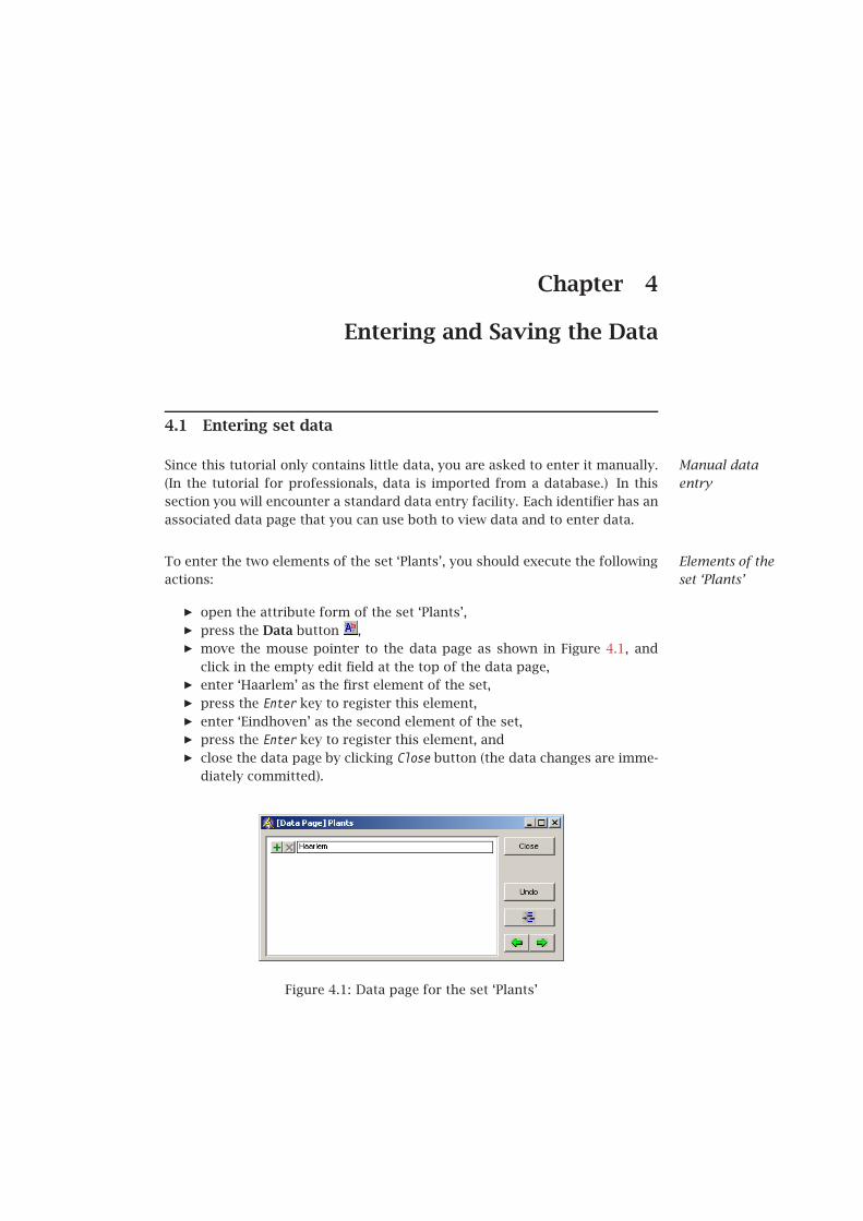
Since this tutorial only contains little data, you are asked to enter it manually.(In the tutorial for professionals, data is imported from a database.) In thissection you will encounter a standard data entry facility. Each identifier has anassociated data page that you can use both to view data and to enter data.

Elements of theset ‘Plants’

To enter the two elements of the set ‘Plants’, you should execute the followingactions:

� open the attribute form of the set ‘Plants’,� press the Data button ,� move the mouse pointer to the data page as shown in Figure 4.1, and

click in the empty edit field at the top of the data page,� enter ‘Haarlem’ as the first element of the set,� press the Enter key to register this element,� enter ‘Eindhoven’ as the second element of the set,� press the Enter key to register this element, and� close the data page by clicking Close button (the data changes are imme-

diately committed).

Figure 4.1: Data page for the set ‘Plants’

Chapter 4. Entering and Saving the Data 22

Changingelement names

To change the name of an element, just, select the element, press the deletebutton and enter the modified name in the same way as described above.

Elements of theset ‘Customers’

The elements of the set ‘Customers’ are entered in exactly the same way as forthe set ‘Plants’. The five elements are listed in Figure 4.2. Note that the lastelement ‘Den Bosch’ contains a blank character.

Figure 4.2: Data page for the set ‘Customers’

4.2 Entering parameter data

Empty tablesThe data page of each indexed parameter is automatically filled with the ele-ments of the corresponding sets. All that is left for you to do, is to enter thenonzero data values.

Supply dataIn order to enter the data for the parameter ‘Supply’, you should execute thefollowing actions (which are similar to the ones described in the previous sec-tion):

� open the attribute form of the parameter ‘Supply’,� press the Data button ,� move the mouse pointer to the first data field and click,� enter the number 47,� press the Enter key to register the first value,� enter the number 63,� press the Enter key to register the second value, and� close the data page by pressing Close button.

Figure 4.3 shows the completed data page of the parameter ‘Supply’.


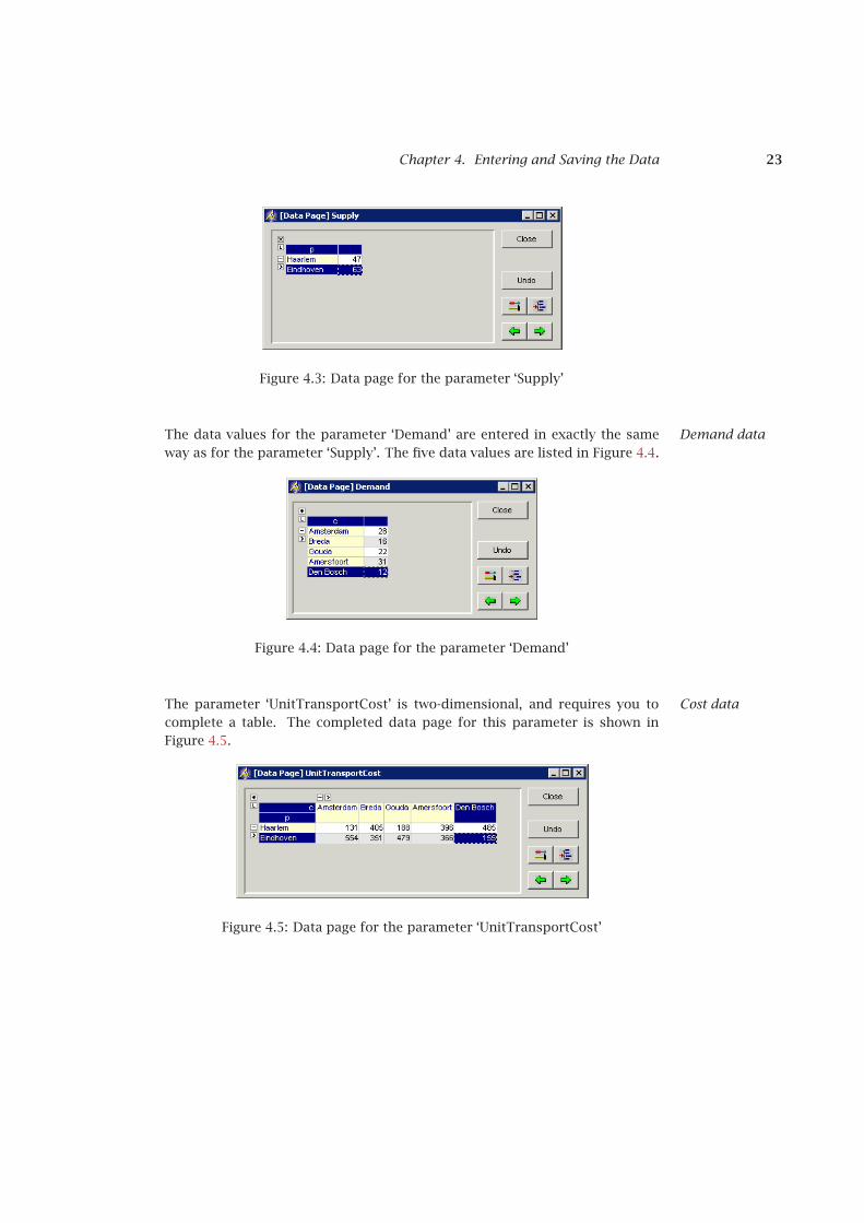
Figure 4.3: Data page for the parameter ‘Supply’

Demand dataThe data values for the parameter ‘Demand’ are entered in exactly the sameway as for the parameter ‘Supply’. The five data values are listed in Figure 4.4.

Figure 4.4: Data page for the parameter ‘Demand’

Cost dataThe parameter ‘UnitTransportCost’ is two-dimensional, and requires you tocomplete a table. The completed data page for this parameter is shown inFigure 4.5.

Figure 4.5: Data page for the parameter ‘UnitTransportCost’


4.3 Saving your data

Casemanagement

Aimms has the option to store the data values of all identifiers in what is re-ferred to as a ‘case’. There are facilities both to save cases and to load cases.

Saving a caseIn order to save the data that you just entered in a new case named ‘Initial BeerTransport Data’, you need to execute the following steps:

� go to the Data menu and execute the Save Case command,� in the Save Case dialog box (see Figure 4.6) enter the name ‘Initial Beer

Transport Data’ in the ‘Name’ field (without the quotes), and� press the Save button to save your data.

Figure 4.6: Save Case dialog box

Loading a caseas the startupcase

If a project in Aimms is closed and subsequently reopened, you may want toreload your data. You may even want Aimms to load a specific case automat-ically each time your project is started. This can be accomplished (withoutprogramming) using the Aimms Options dialog box illustrated in Figure 4.7.

� go to the Settings menu and execute the Project Options command,� select the Project - Startup & Authorization folder in the option tree,� click on the Option Startup Case in the right-most window,� press the wizard button,

� select the case ‘Initial Beer Transport Data’,� press the OK button on the Select Case dialog box,

� press the Apply button on the Aimms Options dialog box, and� finish by pressing the OK button.


Figure 4.7: Aimms options dialog box

Saving yourproject

It is a good habit to save your work regularly. The option settings above arealso saved when you save the entire project. You can save the project bypressing the Save Project button . Note that saving a project does not meanthat the data is also saved. Saving data requires you to save a case.


Loading a casemanually

At any time during an Aimms session you can load a case manually as follows:

� go to the Data menu, select the Load Case submenu and execute the AsActive. . . command,

� select the desired case name in the Load Case dialog box (see Figure 4.8),and

� press the Load button.

Figure 4.8: Load case dialog box

Chapter 5

Solving the Model

5.1 Computing the solution

Procedures foraction

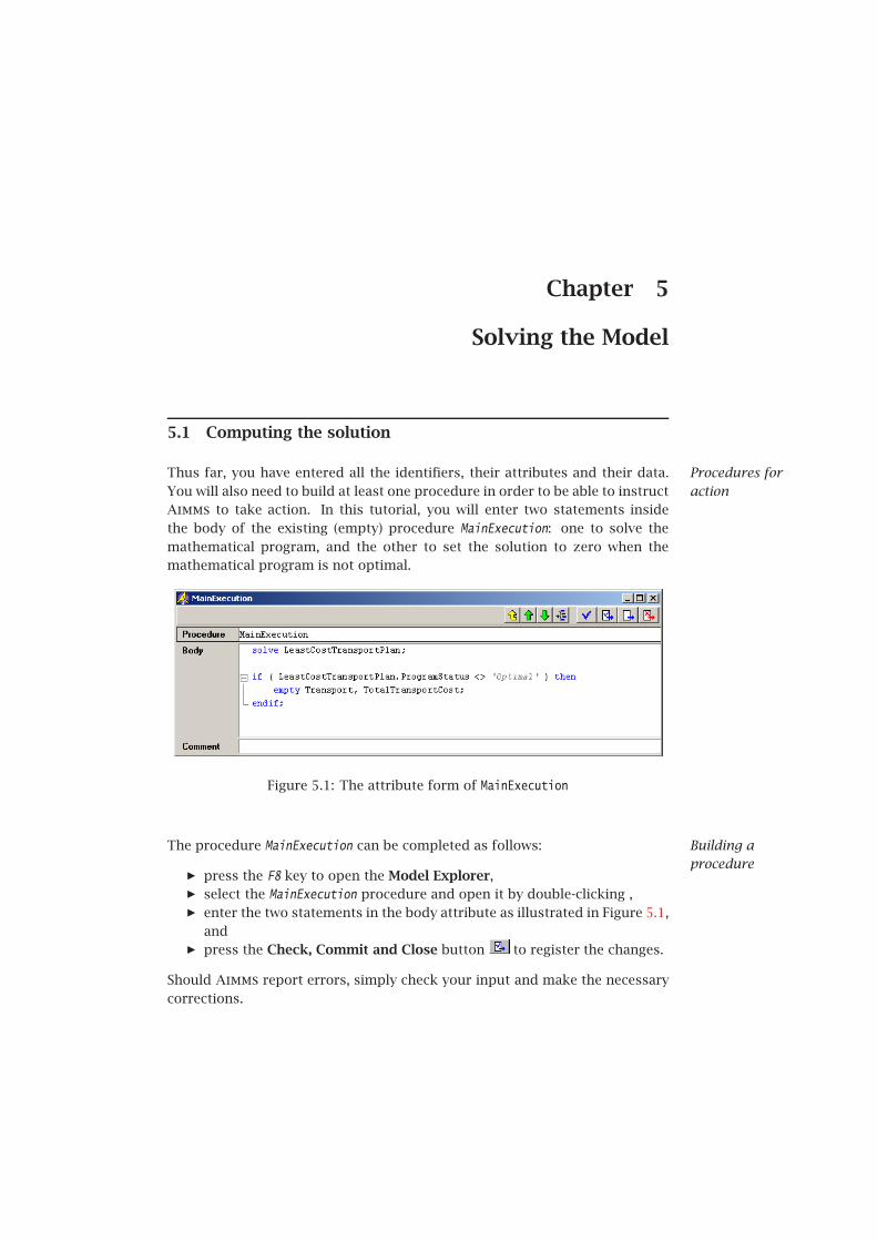
Thus far, you have entered all the identifiers, their attributes and their data.You will also need to build at least one procedure in order to be able to instructAimms to take action. In this tutorial, you will enter two statements insidethe body of the existing (empty) procedure MainExecution: one to solve themathematical program, and the other to set the solution to zero when themathematical program is not optimal.

Figure 5.1: The attribute form of MainExecution

Building aprocedure

The procedure MainExecution can be completed as follows:

� press the F8 key to open the Model Explorer,� select the MainExecution procedure and open it by double-clicking ,� enter the two statements in the body attribute as illustrated in Figure 5.1,

and� press the Check, Commit and Close button to register the changes.

Should Aimms report errors, simply check your input and make the necessarycorrections.

Chapter 5. Solving the Model 28

Right-mouse forhelp

To obtain information about specific Aimms keywords, you can use the right-mouse popup menu to open the Aimms documentation on the appropriatepage with a single click. For instance, you can obtain help on the ‘ProgramSta-tus’ keyword as follows:

� position the cursor over the ‘ProgramStatus’ keyword,� right-click the mouse and select the ‘ProgramStatus’ entry in the ‘Help’

submenu (see Figure 5.2).

Figure 5.2: A right-mouse popup menu

Running theprocedure

The procedure MainExecution is special in that there is a dedicated key, F6, toexecute this procedure. For all other procedures you can use the right mousebutton to select the Run Procedure command.

Watchingexecutionprogress

By pressing the Ctrl and p keys simultaneously, Aimms displays a progresswindow with selected information on the progress it has made (or is making)during an execution phase. Figure 5.3 shows the progress window you shouldexpect to see.

Chapter 5. Solving the Model 29

Figure 5.3: The Aimms progress window

Results in datapages

You have already encountered data pages while entering the elements of setsand the numeric values of parameters. Once Aimms has computed the valuesof the variable ‘Transport’, these values become immediately available on thecorresponding data page. Just go to this variable in the model tree, and clickon it. Then use the right mouse to select the Data. . . command to open the datapage. This will open a pivot table with Transport data and its correspondingsuffices. If you drag the column suffix header out of the pivot table and setthis to level you should see the figure below. Upon closing the data page selectYes, this will save the lay out changes you just made.

Figure 5.4: Data page displaying the solution for the variable ‘Transport’

Chapter 6

Building a Page

Building custompages

Even though Aimms provides standard pages for each identifier, such pages arenot set up to look at groups of related identifiers. That is why model buildersand end-users of an application usually prefer to interact with an applicationthrough one or more custom pages.

6.1 Creating a new page

Using the PageManager

To create a new empty page you should execute the following steps:

� press the Page Manager button on the toolbar,� press the button on the toolbar to create a new page,� specify ‘Beer Transport Input and Output Data’ as the name of this new

page, and� press the Enter key to register the page.

The Page Manager with the new page is shown in Figure 6.1.

Figure 6.1: A Page Manager with a single page

Note that changes made in the previous chapter to the lay out of the Transportdata table are also saved in the Page Manager.

6.2 Presenting the input data

Be aware of twopage modes

A page is either in Edit mode or in User mode. The Edit mode is used forcreating and modifying the objects on a page. The User mode is for viewingand editing the data displayed within objects on a page.

Chapter 6. Building a Page 31

Opening thepage

To open the new page in Edit mode:

� double click on the page name in the Page Manager, and� press the button on the toolbar to open the selected page in Edit mode.

Drawing a newtable . . .

To create a new table, perform the following actions:

� press the new-table button on the toolbar,� position the mouse cursor at where the upper left corner of the new table

should be,� depress the left mouse button and drag the mouse cursor to where the

lower right corner of the new table should be, and� release the mouse button.

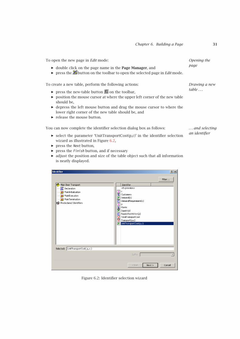
. . . and selectingan identifier

You can now complete the identifier selection dialog box as follows:

� select the parameter ‘UnitTransportCost(p,c)’ in the identifier selectionwizard as illustrated in Figure 6.2,

� press the Next button,� press the Finish button, and if necessary� adjust the position and size of the table object such that all information

is neatly displayed.

Figure 6.2: Identifier selection wizard


Adding supplydata to existingtable

To add another identifier to the ‘UnitTransportCost’ table, execute the follow-ing actions in Edit mode:

� select the table by clicking on it,� press the button on the toolbar (or alternatively, use the right mouse)

to access the properties dialog box,� select the contents tab (see Figure 6.3),� press the Add button,� select the identifier ‘Supply(p)’, press the Next button, and then press the

Finish button, and� back on the contents tab, press the OK button.

Figure 6.3: Table contents tab

Adding demanddata to the table

You can add demand data to the table in the same way as you added the supplydata. The resulting table is shown in Figure 6.4.

Figure 6.4: Table displaying input data


Creating twobar charts

Creating a bar chart is essentially the same process as creating a table. Thefollowing steps summarize the process for the parameter ‘Supply’:

� press the new-bar-chart button on the toolbar,� position the mouse cursor, and drag to form the new bar chart,� select the parameter ‘Supply(p)’ in the identifier selection wizard,� press the Next button, and then the Finish button.

You can then create a bar chart for the demand data in the same way as youcreated the bar chart for the supply data. Your intermediate page should nowlook like the one in Figure 6.5.

Figure 6.5: Intermediate input-output page

6.3 Presenting the output data

Creating acomposite table

A composite table in Aimms is like a relational database table: the first columnscontain indices, and the remaining columns contain identifiers defined overthese indices. Creating a composite table containing only the optimal solutionis similar to creating a standard table or a bar chart, and requires the followingactions:

� press the button on the toolbar to create a new composite table,� draw the table using the mouse,� select the variable ‘Transport(p,c)’ in the identifier selection wizard to

indicate which index values must be displayed,


� press the Next button, and then the Finish button.

Creating astacked barchart

Yet another way to display the solution is by means of a stacked bar chart:

� create a standard bar chart displaying the variable ‘Transport(p,c)’.� select the ‘bar chart’ tab in the properties dialog box as illustrated in

Figure 6.6),� instead of the default ‘Overlapping’ option, select the ‘Stacked Bar’ op-

tion, and� press the OK button.

Figure 6.6: Bar chart property dialog box

Creating ascalar object

The scalar object is designed to display scalar values. To display the optimalsolution value in a scalar object you should do the following:

� press the button on the toolbar to create a scalar object,� draw the scalar object using the mouse,� select the scalar variable ‘TotalTransportCost’ in the identifier selection

wizard, and� press the Finish button.


6.4 Finishing the page

Building awell-organizedoverview

Designing a professional looking graphical end-user interface is not a trivial ac-tivity, and is beyond the scope of this tutorial. Nevertheless, you will be askedto spend a little time building a nice looking page as illustrated in Figure 6.11at the end of this section.

Creating abutton

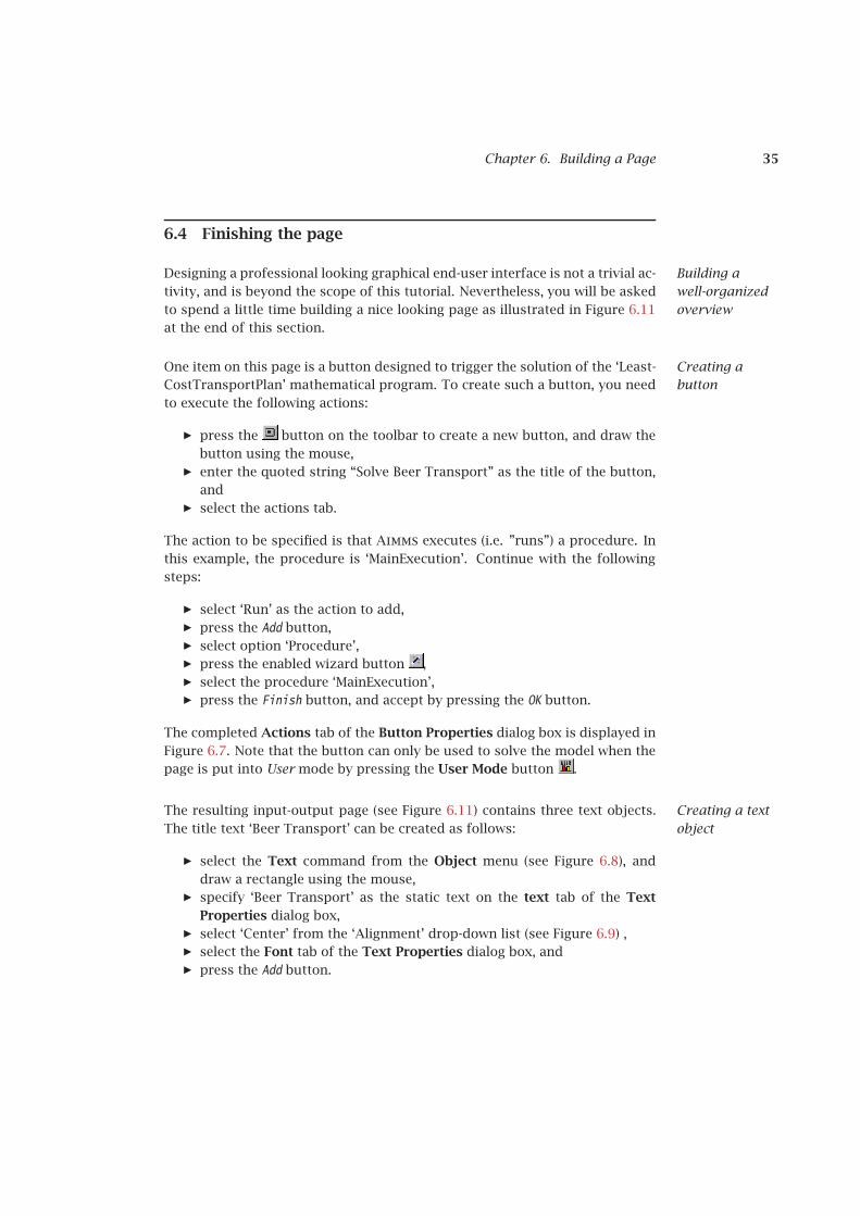
One item on this page is a button designed to trigger the solution of the ‘Least-CostTransportPlan’ mathematical program. To create such a button, you needto execute the following actions:

� press the button on the toolbar to create a new button, and draw thebutton using the mouse,

� enter the quoted string “Solve Beer Transport” as the title of the button,and

� select the actions tab.

The action to be specified is that Aimms executes (i.e. ”runs”) a procedure. Inthis example, the procedure is ‘MainExecution’. Continue with the followingsteps:

� select ‘Run’ as the action to add,� press the Add button,� select option ‘Procedure’,� press the enabled wizard button ,� select the procedure ‘MainExecution’,� press the Finish button, and accept by pressing the OK button.

The completed Actions tab of the Button Properties dialog box is displayed inFigure 6.7. Note that the button can only be used to solve the model when thepage is put into User mode by pressing the User Mode button .

Creating a textobject

The resulting input-output page (see Figure 6.11) contains three text objects.The title text ‘Beer Transport’ can be created as follows:

� select the Text command from the Object menu (see Figure 6.8), anddraw a rectangle using the mouse,

� specify ‘Beer Transport’ as the static text on the text tab of the TextProperties dialog box,

� select ‘Center’ from the ‘Alignment’ drop-down list (see Figure 6.9) ,� select the Font tab of the Text Properties dialog box, and� press the Add button.


Figure 6.7: The action tab of the button properties dialog box

Figure 6.8: The Object menu of a page in Edit mode


Figure 6.9: The text tab of the text properties dialog box

You can now specify and name the appropriate font, and thereby complete thetext object.

� select ‘Bold’ as the Font Style, and ‘20’ as the ‘Font Size’,� press the OK button,� specify ‘Title’ as the name of the new font,� press the OK button to return to the Text Properties tab,� again, press the OK button to leave the Text properties dialog box,

The other two text objects displaying the text ‘Input Data’ and ‘Output Data’are created in the same way. Instead of using the newly constructed ‘Title’font, you should create a second custom font, named ‘Header’ font, of size‘14’. The font tab of the Text Properties dialog box is displayed in Figure 6.10.


Figure 6.10: The font tab of the text properties dialog box

Creating tworectangles

The page is completed by adding two rectangles to emphasize that there aretwo groups of objects representing input data and output data. Assuming thatyou have rearranged and resized the objects to fit neatly together, you candraw the rectangles as follows:

� select the Rectangle command from the Object menu, and� draw the rectangle using the mouse.

Your page should now look like the one in Figure 6.11.


Figure 6.11: An input-output page

Chapter 7

Performing a What-If Run

7.1 Modifying input data

Page user modeHaving developed the input-output page, you are now ready to use the page.For this purpose you must put the page into User mode by pressing the UserMode button .

What-if analysisThe input-output page allows you to see the effect of changes in either thedemand, the supply, or the cost figures of the transport model. Just changeany input data, re-solve the model, and view the resulting output.

Dragging a barchart

For example, to change the available supply in ‘Haarlem’ you can perform thefollowing actions:

� in the ‘Supply’ bar chart, select the bar representing the supply in ‘Haar-lem’,

� position the mouse pointer at the top of the bar, and simply� drag the mouse upwards to increase the supply from 47 to 57 (see Fig-

ure 7.1).

Figure 7.1: The dragging process for supply data illustrated

Chapter 7. Performing a What-If Run 41

Alternatively, you can click on the corresponding bar, and enter the new supplyvalue of 57 in the edit field on the lower left part of the bar chart.

Re-solving themathematicalprogram

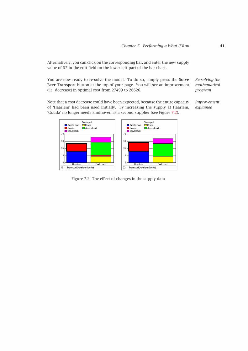
You are now ready to re-solve the model. To do so, simply press the SolveBeer Transport button at the top of your page. You will see an improvement(i.e. decrease) in optimal cost from 27499 to 26626.

Improvementexplained

Note that a cost decrease could have been expected, because the entire capacityof ‘Haarlem’ had been used initially. By increasing the supply at Haarlem,‘Gouda’ no longer needs Eindhoven as a second supplier (see Figure 7.2).

Figure 7.2: The effect of changes in the supply data

Common Aimms Shortcut Keys

Key Function

F1 Open Aimms Help

F2 Rename the selected identifier

F3 Find and repeat find

F4 Switch between edit mode and end-user mode(for the active page)

F5 Compile all

F6 Run MainExecution

Alt+F6 Switch to debugger mode

F7 Save the active page

F8 Open Model Explorer

Ctrl+F8 Open Identifer Selector

F9 Open Page Manager

Alt+ F9 Open Template Manager

Ctrl+ F9 Open Menu Builder

F10 Open Data Manager

Ctrl+ F10 Open Data Management Setup

F11 Open Identifer Info dialog

Ctrl+ B Insert a break point in debugger mode

Ctrl+ D Open Data Page

Ctrl+ F Open Find dialog

Ctrl+ M Open Message Window

Ctrl+ P Open Progress Window

Ctrl+ T View Text Representation of selected part(s)

Ctrl+Shift + T View Text Representation of whole model

Ctrl+ W Open Wizard

Ctrl+ Space Name completion

Ctrl+ Shift+Space Name completion including Aimms PredeclaredIdentifers

Ctrl+ Enter Check, commit, and close

Insert Insert a node (when single insert choice) orOpen Select Node Type dialog (when multipleinsert choices)