ainstitute of economic studies, charles university in prague
TRANSCRIPT

econstorMake Your Publications Visible.
A Service of
zbwLeibniz-InformationszentrumWirtschaftLeibniz Information Centrefor Economics
Dvořáková, Sylvie; Seidler, Jakub
Working Paper
The influence of housing price developments onhousehold consumption: Empirical analysis for theCzech Republic
IES Working Paper, No. 22/2012
Provided in Cooperation with:Charles University, Institute of Economic Studies (IES)
Suggested Citation: Dvořáková, Sylvie; Seidler, Jakub (2012) : The influence of housing pricedevelopments on household consumption: Empirical analysis for the Czech Republic, IESWorking Paper, No. 22/2012, Charles University in Prague, Institute of Economic Studies (IES),Prague
This Version is available at:http://hdl.handle.net/10419/83450
Standard-Nutzungsbedingungen:
Die Dokumente auf EconStor dürfen zu eigenen wissenschaftlichenZwecken und zum Privatgebrauch gespeichert und kopiert werden.
Sie dürfen die Dokumente nicht für öffentliche oder kommerzielleZwecke vervielfältigen, öffentlich ausstellen, öffentlich zugänglichmachen, vertreiben oder anderweitig nutzen.
Sofern die Verfasser die Dokumente unter Open-Content-Lizenzen(insbesondere CC-Lizenzen) zur Verfügung gestellt haben sollten,gelten abweichend von diesen Nutzungsbedingungen die in der dortgenannten Lizenz gewährten Nutzungsrechte.
Terms of use:
Documents in EconStor may be saved and copied for yourpersonal and scholarly purposes.
You are not to copy documents for public or commercialpurposes, to exhibit the documents publicly, to make thempublicly available on the internet, or to distribute or otherwiseuse the documents in public.
If the documents have been made available under an OpenContent Licence (especially Creative Commons Licences), youmay exercise further usage rights as specified in the indicatedlicence.
www.econstor.eu
Institute of Economic Studies, Faculty of Social Sciences
Charles University in Prague
The Influence of Housing Price Developments on
Household Consumption: Empirical Analysis for the
Czech Republic
Sylvie Dvořáková Jakub Seidler
IES Working Paper: 22/2012
Institute of Economic Studies, Faculty of Social Sciences,
Charles University in Prague
[UK FSV – IES]
Opletalova 26 CZ-110 00, Prague
E-mail : [email protected] http://ies.fsv.cuni.cz
Institut ekonomických studií Fakulta sociálních věd
Univerzita Karlova v Praze
Opletalova 26 110 00 Praha 1
E-mail : [email protected]
http://ies.fsv.cuni.cz
Disclaimer: The IES Working Papers is an online paper series for works by the faculty and students of the Institute of Economic Studies, Faculty of Social Sciences, Charles University in Prague, Czech Republic. The papers are peer reviewed, but they are not edited or formatted by the editors. The views expressed in documents served by this site do not reflect the views of the IES or any other Charles University Department. They are the sole property of the respective authors. Additional info at: [email protected] Copyright Notice: Although all documents published by the IES are provided without charge, they are licensed for personal, academic or educational use. All rights are reserved by the authors. Citations: All references to documents served by this site must be appropriately cited. Bibliographic information: Dvořáková, S., Seidler, J. (2012). “The Influence of Housing Price Developments on Household Consumption: Empirical Analysis for the Czech Republic” IES Working Paper 22/2012. IES FSV. Charles University. This paper can be downloaded at: http://ies.fsv.cuni.cz

The Influence of Housing Price Developments on Household
Consumption: Empirical Analysis for the Czech Republic
Sylvie Dvořákováa
Jakub Seidlerb
aInstitute of Economic Studies, Charles University in Prague E-mail: [email protected]
corresponding author
bCzech National Bank and Institute of Economic Studies, Charles University in Prague
July 2012 Abstract: This paper studies how the change of wealth of households represented by housing prices and stock market prices influences households’ consumption. We provide empirical analysis based on the Czech aggregate data from 1998–2009. We analyse the effect of change in households’ wealth on the consumption of both durable and non-durable goods employing the VAR and VEC models on quarterly data. The robustness of results is verified by Dynamic OLS and Fully Modified OLS framework. We find a positive effect of both housing wealth and stock market wealth on both types of consumption. In case of non-durable goods consumption, we estimate the cointegrating vector and conclude that the elasticity of non-durable

goods consumption with respect to housing wealth is over three times greater than with respect to stock market wealth. Keywords: households, housing prices, consumption, housing wealth, stock market wealth, VAR model, VECM JEL: C22, E39, G12 Disclaimer and Acknowledgements: The views expressed in this paper do not necessarily represent those of the abovementioned institutions. Jakub Seidler acknowledges the support from the Czech Science Foundation grant no. P402/12/G097.

1. Introduction This study analyses the relationship between households’ housing wealth and the consumption expenditure of the household sector. This linkage between housing wealth and consumption expenditure drew the attention of many studies in the past two decades, as housing wealth has a unique role in the economy and change in its value can have different implications on the households’ behaviour.
Indeed, similarly to other countries, housing wealth plays a unique role in the Czech Republic. For most households it represents an important anchor and a store of value. Almost four-fifths of the annual increase in the value of all households’ tangible assets is invested into the acquisition of houses or apartments (Dubská, 2009). Moreover, the rising importance of the housing wealth can be demonstrated on the fact that by 2006 households’ total annual investment in housing had tripled compared to 1995 (in nominal terms). Further, in opposite to households stock market wealth (understood as the total value of financial assets), which is supposed to be a sort of luxury good, housing wealth is distributed across income levels groups more evenly (Belsky and Prakken, 2004). As a result, changes of housing prices may have various impacts of the economy and should be therefore analysed in a more detail.
In this study, we focus on and test whether so called “wealth effect” is present in the Czech Republic, i.e. whether a change in housing wealth has a positive influence on the consumption. This effect should be present based on the Modigliani life-cycle hypothesis which supposes that increase of any households’ wealth will result in increase of households’ consumption.
Similar analysis was performed in various countries both on micro and macro data. For instance Dvornak and Kohler (2003) conducted this analysis for Australia, Case et al. (2001) for the U.S. and OECD countries, Belsky and Prakken (2004) also for the U.S., Campbell and Cocco (2004) for the United Kingdom, and Raymon, Man and Choy (2007) for Hong Kong. The wealth effect in these countries was found quite significant. However, there is no unanimous conclusion weather housing wealth or stock market wealth of households is more influential on the consumption. Therefore our study focuses not only on the housing wealth, but also on the stock market wealth of the households.
To the best of our knowledge, there has been only one study dealing with this issue in the Czech Republic (Seč and Zemčík, 2007). However, in opposite to our study, this one was based on micro data. This implies that the analysis of the impact of housing prices on the consumption and the estimation of the magnitude of the housing wealth effect based on aggregate data from the Czech Republic still remains uncovered.
Consequently, our study analyses the relationship between consumption and both housing and stock market wealth based on aggregate data for the period 1998–2009 by applying Vector Autoregression model (VAR) and Vector Error Correction Model (VECM). Because of relatively small sample of employed data, the robustness of obtained results is verified by Dynamic Ordinary Least Squares (DOLS) and Fully Modified OLS (FM-OLS). Contrary to prior beliefs that this effect is not that significant in the Czech Republic,1
Our conclusions in detail are as follows: when estimating VAR on the first differences of the consumption of durable goods we find that the growth of both wealth components indirectly influences growth of consumption through changes in the growth of disposable income. In accordance with the
we find a positive relationship between consumption (both of durable and non-durable goods) and the two wealth components.
1 Since the level of development of the local real estate and financial markets is smaller in the Czech Republic. Also the adjustment of mortgages when housing prices increase is more complicated than for example in the USA, where increase in house prices means higher value of the owned property and thus one can negotiate higher mortgage by using the property as collateral, enabling increased consumption.
2
concept of Impulse Response Function (IRF) we observe that shocks in both wealth components have positive and approximately equal impact on consumption growth. A significant cointegrating vector is found in the VECM concept for the consumption of non-durable goods and services, which indicates the elasticity of consumption of non-durable goods and services with respect to housing wealth (0.18) is over three times greater than with respect to stock market wealth (0.05). In the DOLS and FM-OLS framework, the magnitude of elasticities is smaller, however, the direction of effects remains unchanged. Stronger effect is found in case of non-durable consumption. The effect on consumption of durable goods is rather ambiguous as no direct Granger causality is observed.
The rest of the study is organized as follows. Next section contains a detailed literature overview regarding the topic of housing wealth linkage to the consumption. Chapter 3 provides description of the Czech aggregate data used in our analysis. Following section 4 deals with an econometric analysis based on and estimates regression models for the both type of durable and non-durable consumption. Section 5 provides a discussion regarding the robustness of our results. Conclusion summarizes the results of our analysis.
2. Background and related literature There is quite an extensive literature regarding the influence of housing prices on the consumption. The possible housing prices-consumption linkage comes from the life-cycle hypothesis of saving and consumption, which postulates that all sources of an increase in wealth of household, either in housing or stock market wealth, are supposed to have the same positive effect on household consumption, see Ando and Modigliani (1963).
While the positive effect of housing wealth on the consumption were often confirmed (see further literature), there were raised some doubts whether housing wealth effect and stock market effect should have the same influence on the consumption. As a result, attention of the studies started to be more focused also on distinguishing between these two types of wealth change on the consumption, see Case et al. (2001), Dvornak and Kohler (2003) or Ludwig and Slok (2004). Later, this division began – because of its growing importance – to be commonly applied as the two wealth components need not be necessary similar, contrary to what is proposed by the life-cycle hypothesis of saving and consumption.
The need to distinguish between these two types of effects confirmed also Belsky and Prakken (2004), who claim that home prices are not exposed to the frequent and large fluctuations as the stock market is. Moreover, nominal changes in home values are not that common as nominal changes in stock values, and households feel more secure of gains in housing wealth and thus spend more readily and rapidly when they appear. Other arguments were added by Catte et al. (2004) – if households are liquidity constrained then an increase in housing wealth can make access to credit easier, thus aggregate housing wealth may affect consumption more than an equivalent change in financial wealth. Also Mishkin (2007) argues that the housing wealth effect should be higher than the stock market wealth effect, because housing wealth is spread far more evenly throughout the population. Further, housing prices are far less volatile than stock prices and might be considered longer lasting.
Abovementioned arguments were also confirmed empirically, when Case et al. (2001) found a remarkably higher impact of housing wealth as compared to stock market wealth for a panel of U.S. states and OECD countries. Significant housing wealth effect is also found by Catte et al. (2004) in the United States, Canada, the United Kingdom, Australia, and the Netherlands. However in Italy, Germany or France the effect is rather limited. In the study of Dvornak and Kohler (2003) both stock market wealth and housing wealth are found to have a significant long-run effect on Australian consumption. There was estimated that one percent increase in housing wealth has an effect on aggregate consumption not smaller than the effect of the same increase in stock market wealth. Further, the study of Carroll, Otsuka and

3
Slacalek (2006) also finds evidence for a substantially bigger housing wealth effect compared to the stock market wealth effect based on US aggregate level data. They distinguished between short-run and long-run wealth effects and found that the short-run effect on consumption is relatively small.
On the other hand, also arguments against initial Modigliani hypothesis can be found – although in opposite directions, i.e., that the housing wealth effect should be smaller than other assets’ wealth effects. Mishkin (2007) mentions the bequest motive, and also the fact that if a household is not a homeowner and plans to buy a house in the future, the rise in house prices could even lower its current consumption. Mishkin (2007) and Catte et al. (2004) both agree that when considering which wealth effect – housing or stock market – is higher, the question is rather empirical. The evidence is too ambiguous to confidently reject the standard life-cycle hypothesis, and the equivocality is very often caused by limited data availability. This view is confirmed by other empirical studies, which found positive wealth effect on consumption, but the size of the housing wealth effect is smaller than of the stock market effect.
For example, analysis conducted on aggregate US data by Kishor (2007) estimates cointegration among consumption, labour income, and the two wealth components. He concludes that consumption elasticity with respect to housing wealth is three times smaller than with respect to financial wealth. On the other hand, Ludwig and Slok (2004) say that it is doubtful if the two wealth effects are different. However, they find that there is a long-run relationship between consumption and stock market prices and that the housing wealth effect was larger in the 1985–2000 period than in the 1960–1984 period.
Later in this debate, the distinction between durable and non-durable goods started to be more intensively discussed. According to Ludwig and Slok (2004), non-durable consumption is used in most studies, because durable consumption is considered complementary to investment in stock. However, an argument in favour of including durable goods consumption is the fact that during stock market crashes, it is that, not the consumption of non-durables, which is postponed. Moreover, resources from mortgages are mainly spent on the consumption of durable goods. Belsky and Prakken (2004) and Bostic, Gabriel and Painter (2007) also argue that the two consumption components should be modelled separately, and provide such an analysis. As a result, our study for the Czech Republic distinguishes durable and non-durable consumption.
Having in mind previous results of different studies we see that the positive wealth effect was usually confirmed and the different magnitudes of housing and stock market wealth effect were estimated. However, for example Attanasio et al. (2005) reject the wealth hypothesis based on British individual household level data. They conclude that consumption and house prices tend to be determined by common factors, namely the productivity of labour, and this is the main factor explaining link between housing prices and consumption. This is in contrast with previous studies.
As we can see, mutual comparison of the studies is not often straightforward as different methodology, type of data, or aggregation is used. Some studies are based on individual data samples while other use aggregated data. As our study belongs to the second type of studies, we focused mainly on related literature based on similar aggregated type of data. Even so, the results of presented studies are ambiguous.
However, one study based on micro data must be also mentioned, as this is to the best of our knowledge the only study, dealing with our topic in the Czech Republic. Seč and Zemčík (2007) employed detailed micro data, which allowed them to explicitly distinguish between homeowners and renters, as well as households with and without mortgage. They find that homeowners and renters respond differently to changes in housing prices and rents. A 1% increase in rent lowers a renter’s consumption by 0.25% in comparison with a homeowner. Higher housing prices mean increased consumption of homeowners only. Neither renters nor homeowners respond to changes in mortgage payments. Whether a household
4
is or is not paying a mortgage does not make for significant differences in responding to changes in housing prices, rents or mortgage payments.
3. Data description Data used in this study consists of quarterly observations during the period 1998–2009, which were collected from the Czech Statistical Office (CZSO), the ARAD of the Czech National Bank (CNB), and the Prague Stock Exchange.
As a housing wealth proxy, we use the Residential Property Price Index (RPPI). This index is constructed as a weighted average of family house, apartment, apartment block, and building plot price indices for the whole of the Czech Republic indices based on data available from declarations of real estate transfer tax. The index is calculated from realized purchase prices rather than from supply prices, Dubská (2009).2
When trying to evaluate the impact of changes in housing wealth on consumption, one may posit that the effect is different for homeowners and renters, as was distinguished in Seč and Zemčík (2007). However, according to CZSO, the ratio of renters has been fluctuating around 1/5 of all households. In 2009 for example, it was 22.4%. As a consequence, we use simplifying assumption and do not distinguish between homeowners and renters, we consider all households as homeowners.
Commercial property is not the focus of this paper, and thus it is not included in the analysis.
In this paper, we also distinguish between housing wealth and stock market wealth. However, due to data limitations, we use the stock market price index PX, which is an official index of the Prague Stock Exchange, as a proxy variable for stock market wealth. We consider this index in its average value for one quarter. Use of indices as proxies for the wealth variables is quite common in other studies as well, for example Ludwig and Slok (2004) and Case et al. (2005), however, possible imperfections of indices3
Figure 1
should be considered while interpreting the results. Dynamics of both RPPI and PX indices is displayed in and Figure 2.
2 The supply prices do not reflect the actual realized demand; their role is only being indicative of the overestimation or underestimation of sellers’ expectations. 3 By possible imperfections of RPPI we mean, among others, a substantial delay of the final data publication and the incompleteness of the index. Since only the natural persons, as opposed to juristic persons, are obliged to provide the tax declarations, the information about the sales of new apartments by developers and real estate agencies and the sales of existing apartments by municipalities is missing. It is estimated that one half of all real estate sales is thus omitted (Dubská, 2009).

5
40
60
80
100
120
140
160
-20
-10
0
10
20
98 99 00 01 02 03 04 05 06 07 08 09 10
RPPI, base index=2005RPPI, y-o-y growth, right axis
Figure 1: Evolution of RPPI (left axis – index values, right axis- in %)
Source: CZSO
Figure 2: Evolution of PX index (y axis – index values)
Source: Prague Stock Exchange
Household consumption is available with quarterly frequency both in current and previous-year average prices, by the domestic and national concepts, either in millions of Czech crowns or in the form of indices. For the domestic concept we are able to divide Household Final Consumption Expenditure by Durability into durable, non-durable, and semi-durable goods and services. As a result, we use current price indices with base year 2000 in the domestic concept, which enables us to distinguish between durable and non-durable consumption. The gross disposable income (GDI) is used as a proxy for households’ total income. We also include several other variables, e.g. unemployment, inflation, interest rates (PRIBOR – Prague Interbank Offered Rate), and yields on government bonds, which are used in model specification. Used time series and its transformation are described in the following table.
Table 1: Description of the data
Time series Denotation Data span Note
Consumption of durable goods C_LR 1998 Q4–2009 Q4 Seasonally adjusted
Consumption of non-durable goods and services C_SSR 1998 Q1–2009 Q4 Seasonally adjusted
Gross disposable income GDI 1998 Q1–2009 Q4 Seasonally adjusted
Housing wealth HW 1998 Q1–2009 Q4
Stock market wealth SW 1998 Q1–2009 Q4
Inflation INFLATION 1998 Q1–2009 Q4
Unemployment U 1998 Q1–2009 Q4
3M PRIBOR PRIBOR3 1998 Q1–2009 Q4
Yields from 3M PRIBOR YIELDS3 1998 Q1–2009 Q4
12M PRIBOR PRIBOR12 1998 Q1–2009 Q4
Yields from 12M PRIBOR YIELDS12 1998 Q1–2009 Q4
Yields on five-year government bonds BONDS 2001 Q1–2009 Q4
Source: ARAD, CZSO, Prague Stock Exchange
0
400
800
1200
1600
2000
98 99 00 01 02 03 04 05 06 07 08 09 10
PX - quarter average

6
All variables are indexed (the average of the year 2000 is base year) and transformed to natural logarithms to adjust the data for possible scale effects. Figure 3 illustrates the development of such transformed time series.
4. Model specifications Various types of models and specifications were applied in the aforementioned literature. For instance, Dvornak and Kohler (2003) used panel-data estimation techniques with fixed effects, instrumental variables, and panel Dynamic Ordinary Least Squares (DOLS) estimators. An analysis based on error-correction models was proposed, among others, by Ludwig and Slok (2004), Belsky and Prakken (2004), Case et al. (2005) and Kishor (2007). As regards the analysis in the Czech Republic by Seč and Zemčík (2007), they constructed an unbalanced panel and applied several versions of the pooled OLS model on first differences.
In our analysis, we estimate the Vector Autoregression Model (VAR) for consumption of durable goods (C_LR) and Vector Error Correction Model (VECM) for consumption of non-durable goods (C_SR). The robustness of VECM is checked by Dynamic OLS (DOLS), Fully Modified Ordinary Least Square method (FM-OLS) and Canonical Cointegrating Regression (CCR), see section 5.
Figure 3: Logarithmic transformation of the data (y-axis – logarithmic transformation of time series, year 2000 = base)
Source: ARAD, CZSO, Prague Stock Exchange
While searching for the proper models’ specification, we consider that both durable and non-durable consumption depend on disposable income, housing wealth, stock market wealth, inflation, and unemployment. Also, interest rate as a factor influencing substitution of consumption and savings was used – the three-month PRIBOR in the model of non-durable consumption and yields on government bonds and twelve-month PRIBOR in the durable consumption model. Further, we also constructed yields from real interest rates, in order to avoid negative values of real interest rate computed using Fisher theorem (see Table 1). Due to the possible non-stationarity of employed time series, we perform stationarity tests (see Appendix, Table A7), which results from are used while estimating VAR model.
4.5
4.6
4.7
4.8
4.9
5.0
5.1
98 00 02 04 06 08
C_LR
4.44.54.64.74.84.95.05.15.2
98 00 02 04 06 08
C_SSR
4.44.54.64.74.84.95.05.15.2
98 00 02 04 06 08
GDI
4.4
4.6
4.8
5.0
5.2
5.4
98 00 02 04 06 08
HW
4.0
4.4
4.8
5.2
5.6
6.0
98 00 02 04 06 08
SW
4.504.554.604.654.704.754.804.85
98 00 02 04 06 08
INFLATION
3.83.94.04.14.24.34.44.54.64.7
98 00 02 04 06 08
U
3.23.64.04.44.85.25.66.0
98 00 02 04 06 08
PRIBOR3
4.564.584.604.624.644.664.684.704.72
98 00 02 04 06 08
YIELD3
3.23.64.04.44.85.25.66.0
98 00 02 04 06 08
PRIBOR12
4.52
4.56
4.60
4.64
4.68
4.72
4.76
98 00 02 04 06 08
YIELD12
3.43.63.84.04.24.44.64.8
98 00 02 04 06 08
BONDS

7
4.1. Model for consumption of durable goods We estimated model for consumption of durable goods using the basic p-lag vector autoregressive VAR(p) model in the following form (see e.g. Hamilton, 1994):
(1) (2)
where is an n-dimensional vector generalization of the white noise, Σ is a symmetric positive definite covariance matrix, c is an n-dimensional vector of constants, and denotes an n-dimensional vector of time series variables, namely, . Finally, is an matrix of autoregressive coefficients for each
Several different model specifications were estimated with different combinations of variables and lag lengths. We exclude models which are not stationary and models with serially correlated residuals. The final model’s specification included only four variables, apart from consumption of durable goods (C_LR), there is gross disposable income (GDI), housing wealth (HW) and stock market wealth (SW).
Inflation, unemployment rate, and the interest rate were not significant on the 90% significance level , or if they were, the model did not satisfy its basic assumptions. These results are similar to those of Dvornak and Kohler (2003) or Ludwig and Slok (2004), which do not have abovementioned variables in the final model specification either.
As we intend, however, to examine the long-run relationship among variables, which would be lost by the transition of variables into first differences, we apply the cointegrated VAR model (VECM) if the variables are cointegrated. We test for cointegration by estimating the VAR for the levels and choosing the lag length. Lag length selection criteria indicate 4, 3 and 2 lags (see Table A8 in the Appendix). The models with 4 and 3 lags are not stationary, therefore we work with VAR(2). We then test the levels of the variables for the cointegration using the Johansen cointegration test with 1 lag. When specifying the lag length for the VECM we apply one lag less than are the lags of the VAR, since VECM is specified for first differences. Since no cointegrating relation is found (see Table A9 in the Appendix), we estimate VAR model only. The absence of cointegration is also confirmed by applying various specification of the DOLS and FM-OLS framework.4
As a consequence, we estimate the VAR(1) model based on lag length selection criteria (see
Table A10 in the Appendix) in the following form:
Equations for the three other variables can be expressed analogously. The results of our regression are presented in the following table.
Table 2: VAR(1) for consumption of durable goods
ΔC_LRt ΔGDIt ΔHWt ΔSWt ΔC_LR t-1 0.388909* 0.044551 -0.197276 0.350725 (0.14017) (0.12961) (0.16109) (1.39448) [ 2.77454] [ 0.34374] [-1.22465] [ 0.25151] ΔGDI t-1 0.403712* -0.198013 0.100790 -2.076778 (0.15403) (0.14242) (0.17701) (1.53235) [ 2.62100] [-1.39033] [ 0.56939] [-1.35529]
4 The results are not presented in the paper, however, they are available upon request.

8
ΔHW t-1 0.067783 0.286980* 0.783822* -0.706578 (0.11287) (0.10436) (0.12971) (1.12288) [ 0.60054] [ 2.74980] [ 6.04274] [-0.62925] ΔSW t-1 0.000870 0.054025* 0.027822 0.373935* (0.01451) (0.01342) (0.01667) (0.14434) [ 0.05993] [ 4.02697] [ 1.66857] [ 2.59058] C -0.001336 0.010187* 0.003945 0.056028* (0.00281) (0.00259) (0.00322) (0.02791) [-0.47612] [ 3.92766] [ 1.22372] [ 2.00767] Notes: Standard errors in ( ) & t-statistics in [ ], * denotes 95% significance level.
All model assumptions are satisfied (we tested for the model stationarity and serial correlation of the residuals, heteroskedasticity and normality).5
Table 2
illustrates that the quarterly growth of consumption depends on its lagged value and on the quarterly growth of disposable income and does not depend on changes in the growth of housing and stock market wealth. However, these two variables are significant for explaining the growth of disposable income, so we observe just an indirect positive link between consumption and housing and stock market wealth. This is confirmed also by Granger causality illustrating on the 95% significance level that changes in both wealth components Granger cause changes in disposable income, which also Granger cause changes in consumption (Table A11 in the Appendix).
Figure 4: Response to Cholesky One S.D. Innovations ± 2 S.E. (Consumption of durable goods, y-axis – response, x-axis – time in quarters)
Source: ARAD, CZSO, Prague Stock Exchange, Author’s calculations
Further, we examine this framework by IRF, where the impulse is one standard deviation to the error term. Figure 4 shows that the growth of consumptions responds positively to shocks in all variables and the shocks eventually dissipate, which confirms the stability of the model. An increase in the growth of 5 The test results are not presented in the paper, however, they are available upon request.

9
disposable income causes a gradual increase in the growth of consumption for two quarters, when it reaches its peak. Then the growth of consumption slows down, and the effect of the shock disappears after one year. The reaction to changes in growth of the two wealth components is lower in magnitude and also it takes more time for the shock to fully manifest itself and to die out. The highest impact can be seen after three quarters and the shock wears off after approximately two and a half years. Thus we conclude that changes in housing wealth and stock market wealth have a positive impact on changes in consumption.
In Figure 5, the growth of stock market wealth has a bigger impact on the growth of disposable income than the growth of housing wealth (by almost 50%). Both effects manifest themselves quite quickly and reach the peak after two quarters. The effect of housing wealth is slightly longer lasting, however both impulses dies out after two years.
Figure 5: Response to Cholesky One S.D. Innovations ± 2 S.E. (Gross Disposable Income, y-axis – response, x-axis – time in quarters)
Source: ARAD, CZSO, Prague Stock Exchange, Author’s calculations
4.2. Model for consumption of non-durable goods
In this section, the relation between the consumption of non-durable goods and services and other variables is estimated. It is assumed that the relations should be slightly different for the two types of consumption.
We estimate several different specifications of the model with various combinations of variables and lag lengths; however we again end up with the basic model with four variables: consumption of non-durable goods and services (C_SSR), gross disposable income (GDI), housing wealth (HW), and stock market wealth (SW).
Because of non-stationarity of employed time series, we test again for cointegration. First, we estimate VAR model for the levels, and estimate the lag length. Then we perform the Johansen cointegration test with one lag less. All lag length selection criteria chose 2 lags for the variables in levels (see Table A12 in the Appendix), thus we apply the Johansen cointegration test on 1 lag (since it works on first differences). The test for cointegration strongly depends on deterministic trend assumptions. According to Juselius (2006) there are five cases to consider. The first two cases do not allow for a deterministic trend in the data, another two allow for a linear trend, and the last one allows for a quadratic trend in data. We choose case number three,6
Table A13
which assumes a linear trend (and an intercept) in the data and an intercept and no linear trend in VAR. This means that in the cointegrating equation there is only intercept and no trend. The results of the test are presented in in the Appendix. Both Trace statistics and Maximum Eigenvalue statistics indicate one cointegrating vector.
6 We applied this case also in the previous subchapter, where we tested for cointegration.

10
In this case, applying the VAR model on stationary first differences means a loss of long-run equilibrium information and thus we focus only on the VECM.
We estimate the long-term relationship among variables after stabilization in a steady state, where the growth of variables per given time units is close to zero (Cipra, 2008).
We estimate the corrected model in the following form:
(3)
The vector of coefficients describes the short-term relationships among variables, the vector describes long-term cointegration relationship, and finally coefficient stands for the speed of adjustment and for the intercept in the cointegration relation. The other three equations can be expressed analogously.
The Eq.4, compared to the Eg.3, furthermore contains the error-correction term:
(4)
This term is constructed from the lagged values of the variables in levels (as opposed to first differences). This model describes short-term relationships between the growth components (for example between
and ), but also provides correction for the case when short-term changes make the levels of the variables deviate from their long-run equilibrium. If the correction term is the cointegrating relation, then all variables in the model are stationary and the regression can be consistently estimated using OLS.
The estimated model is displayed in the following table.
Table 3: VECM for consumption of non-durable goods
Cointegrating Eq: C_SSR(-1) GDI(-1) HW(-1) SW(-1) C
CointEq1 1.000000 -0.552294 -0.179079 -0.053481 -1.000818
(0.10718) (0.06372) (0.01212)
[-5.15272] [-2.81039] [-4.41106]
Error Correction: ΔC_SSRt Δ GDIt Δ HWt Δ SWt CointEq1 -0.331314 -0.094652 0.265703 1.519020 (0.08160) (0.11068) (0.12447) (1.14483) [-4.06021] [-0.85516] [ 2.13465] [ 1.32685] Δ C_SSRt-1 0.057229 0.213836 0.433622 1.811176 (0.14775) (0.20041) (0.22538) (2.07296) [ 0.38733] [ 1.06697] [ 1.92394] [ 0.87372] Δ GDI t-1 -0.132493 -0.269623 0.140770 -1.997902 (0.12357) (0.16761) (0.18849) (1.73364) [-1.07222] [-1.60864] [ 0.74683] [-1.15243] Δ HW t-1 0.032862 0.249198 0.740734 -0.140427 (0.06923) (0.09390) (0.10560) (0.97122) [ 0.47471] [ 2.65393] [ 7.01486] [-0.14459] Δ SW t-1 -0.001676 0.055867 0.039090 0.463071 (0.01004) (0.01362) (0.01532) (0.14092) [-0.16687] [ 4.10044] [ 2.55127] [ 3.28597] C 0.013319 0.009643 -0.003564 0.018462 (0.00241) (0.00327) (0.00368) (0.03386) [ 5.51873] [ 2.94588] [-0.96799] [ 0.54527]

11
Notes: Standard errors in ( ) & t-statistics in [ ], * denotes 95% significance level.
All demanded assumptions of the model are fulfilled.7
The estimated cointegrating vector is the result of the first step of the Johansen procedure. Since the dependent and the explanatory variables are in natural logarithms, the interpretation of the cointegrating vector is in terms of elasticities (Kishor, 2007). We can conclude that the long-run elasticity of consumption of non-durable goods and services with respect to housing wealth (0.18) is over three times greater than the elasticity with respect to financial wealth (0.05). These results do not stand out among results obtained by other studies. In particular the elasticity with respect to housing wealth lies in the interval proposed by Attanasio et al. (2005).
We find a significant cointegrating vector whose unique identification is achieved by applying a normalizing assumption.
Results of VECM in Table 3 indicate that in the regression of consumption the short-term relationships are not significant, but the long-term relationships expressed by the cointegrating vector are. The consumption of non-durable goods and services responds positively in the long run to disposable income and to both wealth components. Based on the values of the elements of the cointegrating vector, the elasticity of consumption with respect to housing wealth is over three times greater than with respect to stock market wealth. It means households are more sensitive to changes in housing prices. On the other hand, changes in disposable income are in the short run strongly and positively influenced by changes in housing and stock market wealth. In models for both types of consumption the housing wealth and stock market wealth have positive and significant impact on gross disposable income and on consumption as well.
Comparison of results across studies, even if they apply VECM and are testing for cointegration, is not straightforward, as different types of data and model specifications are set. The most similar choice and type of variables and estimation procedure is presented in the study of Kishor (2007), who assesses whether the housing wealth effect or the stock market wealth effect influence consumption in the USA (in this study, the consumption of nondurable goods and services is supposed to be influenced by labour income, housing wealth and financial market wealth).
However, Kishor concludes the very opposite than our study. The elasticity of consumption with respect to financial wealth is approximately three times greater than with respect to housing wealth. These opposite results, mainly due to a considerably small stock market wealth effect in the Czech Republic, might be caused by the different characteristics of the American and Czech stock markets and rather underdeveloped financial market in the Czech Republic. Elasticities with respect to labour income are roughly similar; however theory suggests they should be close to one. It means we have found that the consumption of non-durable goods and services in the Czech Republic responds less to changes in labour income than it does in the USA.
5. Robustness of the results We have applied the vector error correction model for estimating model for consumption of non-durable goods in the previous section. However, as this method may obtain biased results – especially in the small samples – we also use the Dynamic OLS (DOLS), Fully Modified Ordinary Least Square method (FM-OLS) and Canonical Cointegrating Regression (CCR) as the robustness check of presented Johansen’s results.
FM-OLS estimating the cointegration by triangular system representation was developed by Phillips and Hansen (1990). The traditional OLS was modified to account for possible serial correlation and 7 The test results are not presented here because of space limitation, but they are available upon request.
12
endogeneity. Similar method was also proposed by Stock and Watson (1993), in the case of 1 cointegrating vector and I(1) process, so called Dynamic OLS (DOLS) means simply “regressing one of the variables onto the contemporaneous levels of remaining variables, leads and lags of their first differences and a constant, using either OLS or GLS”.8
According to Phillips (1994) all abovementioned methods are asymptotically equivalent, however this does not hold for finite samples. Gregory (1994) presents an evaluation of the finite-sample performance of several tests for cointegration. Using Monte Carlo design to evaluate the tests’ performance, the overall conclusion is that tests produce roughly similar results when the number of observation is around 50 and number of regressors . The problem arises when the number of regressors and observations increases. Powers of the tests keep falling with increasing k. In our case, , which, based on Gregory (1994) results, should cause the cointegration tests results to vary sharply.
This estimate of cointegrating vector is asymptotically efficient.
Phillips (1994) concludes that the Johansen procedure may be unreliable in sense of being an extreme outlier and mentions one possible explanation for the observed outlier behaviour. Phillips (1994) states that under certain condition, the density of reduced rank regression estimator has Cauchy-like tail behaviour and thus does not have finite first moments. On the other hand, the triangular system representation has finite moments until – , where is number of observations, represents full rank integrated regressors.
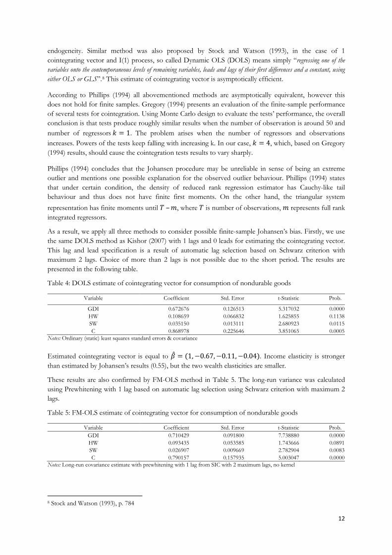
As a result, we apply all three methods to consider possible finite-sample Johansen’s bias. Firstly, we use the same DOLS method as Kishor (2007) with 1 lags and 0 leads for estimating the cointegrating vector. This lag and lead specification is a result of automatic lag selection based on Schwarz criterion with maximum 2 lags. Choice of more than 2 lags is not possible due to the short period. The results are presented in the following table.
Table 4: DOLS estimate of cointegrating vector for consumption of nondurable goods
Variable Coefficient Std. Error t-Statistic Prob.
GDI 0.672676 0.126513 5.317032 0.0000 HW 0.108659 0.066832 1.625855 0.1138 SW 0.035150 0.013111 2.680923 0.0115 C 0.868978 0.225646 3.851065 0.0005
Notes: Ordinary (static) least squares standard errors & covariance
Estimated cointegrating vector is equal to . Income elasticity is stronger than estimated by Johansen’s results (0.55), but the two wealth elasticities are smaller.
These results are also confirmed by FM-OLS method in Table 5. The long-run variance was calculated using Prewhitening with 1 lag based on automatic lag selection using Schwarz criterion with maximum 2 lags.
Table 5: FM-OLS estimate of cointegrating vector for consumption of nondurable goods
Variable Coefficient Std. Error t-Statistic Prob. GDI 0.710429 0.091800 7.738880 0.0000 HW 0.093435 0.053585 1.743666 0.0891 SW 0.026907 0.009669 2.782904 0.0083 C 0.790157 0.157935 5.003047 0.0000
Notes: Long-run covariance estimate with prewhitening with 1 lag from SIC with 2 maximum lags, no kernel
8 Stock and Watson (1993), p. 784

13
We find a cointegrating vector as . Income elasticity is even stronger and is significant on 1% level of significance. Stock market wealth elasticity is also significant on 1% but is smaller compared to Johansen procedure (0.05) and to DOLS estimates (0.04).
Finally, we perform a Canonical Cointegrating Regression (Park, 1992), which confirms the most the Johansen’s procedure results. The estimation setting is exactly the same as for the FM-OLS.
Table 6: CCR estimate of cointegrating vector for consumption of nondurable
Variable Coefficient Std. Error t-Statistic Prob. GDI 0.563327 0.135096 4.169837 0.0002 HW 0.164975 0.072002 2.291248 0.0274 SW 0.041430 0.013251 3.126575 0.0033 C 1.071151 0.242389 4.419141 0.0001
Notes: Long-run covariance estimate with prewhitening with 1 lag from SIC with 2 maximum lags, no kernel
Cointegrating vector is . This vector is significant on 5% level of significance and confirms the original Johansen’s results.
Based on the estimated regressions we conclude that the results from Johansen (1988) method are confirmed by all mentioned methods, which are more suitable for finite-samples. Despite small differences across all estimated models, the interpretation of the initially obtained results remains valid.9
Even if our results indicate statistically positive relationship between housing and stock prices development and the households’ consumption of both durable and non-durable goods, we are aware that this identified effect may be present as a consequence of economic cycle. An increase of economic performance connected with the increase of households’ real income and optimistic future prospects may result in higher demand for both housing property and consumption. The empirical identification of causality may be still questioned because of the quality of employed data, insufficient frequency or relatively small length of time series. These caveats must be considered even in the case of our study.
Nevertheless, the positive linkage between housing prices and consumption may be still explained by the possible use of property as collateral, which enables households to take the loan more easily and thus finance their consumption. This possible link may have become more important even in the Czech Republic, since banks introduced so called American type mortgages in 2004, which are not conditioned by the housing purchase, however, households’ property is used as collateral.
Effect of using housing property as collateral may also be related to the refinancing mortgage with the fixed-rate. If the interest rates decrease during the time of its fixed-rate period, borrowers can easily refinance (pay back) their residual value of initial mortgages by taking new mortgage for better rates (mainly at the end of the fixed-rate period, when mortgages could be repaid without substantial fees). However, banks may offer borrower willing to refinance its mortgage higher amount of the new mortgage than is its residual value, which enables households to get easily additional loan and increase their consumption. The amount of additional value of loan will depend also – among others – on the value of the property used as a collateral, and will increase with the housing prices growth.
This effect may be more relevant especially nowadays, when low interest rate lead to the significant amount of refinanced mortgages. In the long lasting environment of low interest rate this effect may become even more important, which should be addressed in the future research.
9 Estimates for FM-OLS, DOLS and CCR are presented for 1998–2008 period only since including year 2009 lead to less persuasive results, which could be resulted by the materialization of the financial crisis in the Czech Republic in 2009 and significant structural break.

14
6. Conclusion In this study we present an analysis of how housing prices influence the consumption of households. To the best of our knowledge, this analysis on aggregate data has not been conducted in the Czech Republic so far.
We assume that an increase in housing prices or an equivalent increase in housing wealth should significantly influence consumption. We divide total household wealth into two components: housing wealth and stock market wealth. We also distinguish between the consumption of durable goods and of non-durable goods and services, as the literature has some ambiguity about which consumption should be used.
We apply the VAR model on Czech quarterly data from the period 1998–2009, and in case of cointegration we use the VECM. We include several variables though relevant into our analysis: consumption, disposable income, housing wealth, stock market wealth, interest rate, unemployment, inflation, and yields on government bonds. The final models, however, include only the first four variables mentioned.
We use the Residential Property Price Index as a proxy for housing wealth and the Prague stock market index as a proxy for stock market wealth. We are aware that the quality of employed data is a limitation, which should be considered when interpreting our results. However, use of indices as proxies for the wealth variables is the consequence of limited other data sources and is common in other studies dealing with similar problematic.10
The VAR model is applied for the consumption of durable goods. We find a positive indirect wealth effect stemming from changes in housing wealth and stock market wealth (supported by the Granger causality test and IRF). However, this result should be taken with caution, since no direct evidence is observed.
Since in the model of consumption of non-durable goods and services the variables are cointegrated, the VAR model specified in the first differences is omitting the long-run relationship and is explaining only the short-term adjustments. As a result, we estimate the cointegrating vector for the consumption of non-durable goods and conclude that the elasticity of consumption of non-durable goods and services with respect to housing wealth (0.18) is over three times greater than with respect to stock market wealth (0.05). The robustness of these results is confirmed with slightly smaller magnitude by DOLS and FM-OLS framework.
The study concludes that there is a positive linkage between property prices and households consumption in the Czech Republic as we found a statistically significant both housing and stock market wealth effect especially for the consumption of non-durable goods.
10 For example Ludwig and Slok (2004), Case et al. (2005), or Hlaváček and Komárek (2011).

15
References
Ando, A. and F. Modigliani (1963) “The 'Life-Cycle' Hypothesis of Saving: Aggregate Implications and Tests,” American Economic Review, Vol. 53 (March), pp. 55–84. Attanasio, O., L. Blow, R. Hamilton, and A. Leicester (2005) “Consumption, House Prices, and Expectations,” Bank of England Working Paper No. 271 (London: Bank of England, September). Belsky, E. and J. Prakken (2004) “Housing Wealth Effects: Housing's Impact on Wealth Accumulation, Wealth Distribution and Consumer Spending,” (Chicago: National Centre for Real Estate Research). Bostic, R., S. Gabriel, and G. Painter (2007) “Housing Wealth, Financial Wealth, and Consumption: New Evidence from Micro Data,” Regional Science and Urban Economics, Vol. 39, No. 1, January 2009. Case, K.E., J.M. Quigley, and R.J. Shiller (2001) “Comparing Wealth Effects: The Stock Market Versus the Housing Market,” NBER Working Paper No. 8606. Case, K.E., J.M. Quigley, and R.J. Shiller (2005) “Comparing Wealth Effects: The Stock Market Versus the Housing Market,” Advances in Macroeconomics, Vol. 5, No. 1. Campbell, J. Y. and J. F. Cocco (2004) “How do house prices affect consumption? Evidence from micro data,” Journal of Monetary Economics, Vol. 54, No. 3, 591–621. Carroll, C., M. Otsuka, and J. Slacalek (2006) “How Large is the Housing Wealth Effect? A New Approach,” NBER Working Paper No. 12746 (Cambridge, Mass.: National Bureau of Economic Research, December). Catte, P., N. Girouard, R. Price, and C. Andre (2004) “Housing Markets, Wealth, and the Business Cycle,” OECD Economics Department Working Papers No. 394, OECD Publishing. Cipra, T. (2008) “Finanční ekonometrie” (Financial Econometrics), first edition, Ekopress 2008. CNB (2011) – data series system ARAD Available at http://www.cnb.cz/docs/ARADY/HTML/index_en.htm. CZSO (2011) – time series and Business cycle survey Available at http://www.czso.cz/ and http://www.czso.cz/eng/redakce.nsf/i/business_cycle_surveys. Dubská, D. (2009) “Realitní trh České republiky: cenová bublina ano či ne? (Czech real estate market: price bubble, yes or not?) “, Analysis, Czech Statistical Office, July 2009. Dvornak, N. and M. Kohler (2003) “Housing wealth, stock market wealth and consumption: A panel analysis for Australia,” Research Discussion Paper No., 2003–07, Economic Research Department, Reserve Bank of Australia. Gregory, A. W. (1994), Testing for Cointegration in Linear Quadratic Models, Journal of Business & Economic Statistics, Vol. 12, No. 3 (Jul., 1994), 347–360. Hamilton, D. J. (1994) “Time series analysis,” Princeton University Press, Princeton, New Jersey 1994. Hlaváček, M. and L. Komárek (2011) “Regional Analysis of Housing Price Bubbles and Their Determinants in the Czech Republic”, Czech Journal of Economic and Finance, Vol. 61, No. 1., 2011. Johansen, S. and K.. Juselius (1990). Maximum Likelihood Estimation and Inference on Cointegration with Applications to the Demand of Money, Oxford Bulletin of Economics and Statistics, 52, 169–210. Johansen, S. (1988), Statistical analysis of cointegration vectors, Journal of Economic Dynamics and Control, Vol. 12, Issues 2–3, June–September 1988, Pages 231–254. Juselius, K. (2006) “The Cointegrated VAR model, Methodology and Applications,” Oxford University Press, 2006. Kishor, N. K. (2007) “Does Consumption Respond More to Housing Wealth Than to Financial Market Wealth? If So, Why?” Journal of Real Estate Finance and Economics, Vol. 35 No. 4, 427–48. Park, J. Y. (1992). “Canonical Cointegrating Regressions,” Econometrica, 60, 119–143.

16
Phillips, P. C. B. and B. E. Hansen (1990). Statistical Inference in Instrumental Variables Regression with I(1) Processes, Review of Economics Studies, Vol. 57, 99–125. Phillips, P. C. B. (1994), Some Exact Distribution Theory for Maximum Likelihood Estimators of Cointegrating Coefficients in Error Correction Models, Econometrica Vol. 62, No. 1, 73–93. Prague Stock Exchange (2011) – PX index data series, available at http://www.pse.cz or at http://www.bcpp.cz/On-Line/Indexy/. Ludwig, A. and T. Slock (2004) “The relationship between stock prices, house prices and consumption in OECD countries,” Topics in Macroeconomics, Vol. 4, Issue 1, Article 4. Mishkin, F. S. (2007) “Housing and the Monetary Transmission Mechanism,” NBER Working Paper No. 13518. Raymond Y.C. Tse, K.F. Man, L. Choy (2007) “The impact of Housing and Financial Wealth on Household Consumption: Evidence from Hong Kong,” Journal of Real Estate Literature, Vol. 15, No. 3. Seč, R. and P. Zemčík (2007) “The impact of Mortgages, House Prices and Rents on Household Consumption in the Czech Republic,” CERGE-EI Discussion Paper 2007–185. Stock, J. H. and M. Watson (1993). A Simple Estimator Of Cointegrating Vectors In Higher Order Integrated Systems, Econometrica, 61, 783-820. .

17
Appendix:
Unit root tests
For the unit root testing, we apply the Augmented Dickey-Fuller test, which allows for the residuals to be serially correlated and it can be applied on more complicated dynamic structures (compared to the Dickey-Fuller Test). The lag length selection criteria are employed (the BIC and Modified Akaike criterion – MAIC). In case of ambiguity, we look at the ACF and PACF functions to decide the lag length, and then apply the test again (the graphs indicate mostly AR(1) processes). The results of ADF test based on MAIC criterion may be seen in Table A7.
Based on the results of the ADF Unit Root tests, where all p-values are larger than 0.05, we do not reject the null hypothesis of non-stationarity. We also conduct the KPSS test,11
Table A7
which supports our conclusions, and we therefore reject the null hypothesis of stationarity on the 5% level of significance. We then test the first differences for unit root (see ).
Based on the ADF test we reject the null hypothesis of unit root on the 5% level of significance. Thus we consider our original time series as difference stationary (I(1)) processes.
Table A7: ADF Unit Root tests on levels and on first differences
Series Prob. Lag Series Prob. Lag
C_LR 0.6979 1 ΔC_LR(no intercept) 0.0352 1
C_SSR 0.8039 0 ΔC_SSR 0.0297 1
GDI 0.6453 0 ΔGDI 0.0047 1
HW 0.5752 2 ΔHW(1 fixed lag) 0.0137 1
SW 0.7923 2 ΔSW 0.0008 0
INFLATION 0.5620 0 ΔINFLATION 0.0000 0
U 0.3346 3 ΔU(no intercept) 0.0173 1
PRIBOR3 0.2067 1 ΔPRIBOR3 0.0252 1
YIELD3 0.0941 2 ΔYIELDS3 0.0000 0
PRIBOR12 0.4935 0 ΔPRIBOR12 0.0003 0
YIELD12 0.5678 4 ΔYIELDS12 0.0007 0
BONDS 0.6409 0 ΔBONDS 0.0003 0
Notes: Individual effects, individual linear trends used as exogenous variables
Consumption of durable goods
Table A8: VAR Lag Order Selection Criteria for levels
Lag AIC SC HQ 0 -8.074451 -7.907274 -8.013574 1 -18.19694 -17.36105 -17.89256 2 -19.43023 -17.92563* -18.88234 3 -19.69681 -17.52350 -18.90541* 4 -19.82962* -16.98759 -18.79471 Notes: * indicates lag order selected by the criterion, AIC: Akaike information criterion, SC: Schwarz information criterion, HQ: Hannan-Quinn information criterion Endogenous variables: C_LR, GDI, HW, SW and a constant..
11 Test results are not included in this study, but are available upon request.

18
Table A9: Johansen test for cointegration with linear trend in the data
Unrestricted Cointegration Rank Test (Trace) Hypothesized Trace 0.05 No. of CE(s) Eigenvalue Statistic Critical Value Prob.** None 0.447124 45.71478 47.85613 0.0784 At most 1 0.203249 20.23208 29.79707 0.4073 At most 2 0.195998 10.46191 15.49471 0.2469 At most 3 0.024833 1.081294 3.841466 0.2984 Unrestricted Cointegration Rank Test (Maximum Eigenvalue) Hypothesized Max-Eigen 0.05 No. of CE(s) Eigenvalue Statistic Critical Value Prob.**
None 0.447124 25.48269 27.58434 0.0907 At most 1 0.203249 9.770179 21.13162 0.7659 At most 2 0.195998 9.380612 14.26460 0.2558 At most 3 0.024833 1.081294 3.841466 0.2984 Notes: 1 lag in fist differences, * denotes rejection of the hypothesis on 95% significance level, **MacKinnon-Haug-Michelis (1999) p-values. Neither Trace test nor Max-eigenvalue test indicates cointegration on 95% significance level. Series: C_LR, GDI, HW and SW.
Table A10: VAR Lag Order Selection Criteria for first differences
Lag AIC SC HQ 0 -17.74495 -17.57606 -17.68388 1 -19.09328* -18.24884* -18.78796* 2 -18.87835 -17.35836 -18.32877 3 -18.59949 -16.40395 -17.80565 4 -18.77120 -15.90010 -17.73310 Notes: * indicates lag order selected by the criterion, AIC: Akaike information criterion, SC: Schwarz information criterion, HQ: Hannan-Quinn information criterion, Endogenous variables: ΔC_LR, ΔGDI, ΔHW, ΔSW and a constant.
Table A11 : VAR Granger Causality/Block Exogeneity Wald Tests
Dependent variable: ΔC_LR Excluded Chi-sq df Prob. ΔGDI 6.869646 1 0.0088 ΔHW 0.360649 1 0.5481 ΔSW 0.003592 1 0.9522 All 10.86819 3 0.0125 Dependent variable: ΔGDI Excluded Chi-sq df Prob. ΔC_LR 0.118157 1 0.7310 ΔHW 7.561378 1 0.0060 ΔSW 16.21651 1 0.0001 All 25.53558 3 0.0000

19
Consumption of non-durable goods and services
Table A12: VAR Lag Order Selection Criteria for the levels
Lag AIC SC HQ
0 -9.169961 -9.007762 -9.109810 1 -19.41249 -18.60149 -19.11173 2 -20.2005* -18.74071* -19.65914* 3 -19.80376 -17.69518 -19.02180 4 -19.84889 -17.09150 -18.82632 Notes: * indicates lag order selected by the criterion, AIC: Akaike information criterion, SC: Schwarz information criterion, HQ: Hannan-Quinn information criterion Endogenous variables: C_SSR, GDI, HW, SW and a constant.
Table A13: Johansen test for cointegration with linear trend in the data
Unrestricted Cointegration Rank Test (Trace) Hypothesized Trace 0.05 No. of CE(s) Eigenvalue Statistic Critical Value Prob.** None 0.480076 48.88638 47.85613 0.0399 At most 1 0.192312 18.79903 29.79707 0.5074 At most 2 0.135433 8.974362 15.49471 0.3678 At most 3 0.048359 2.280123 3.841466 0.1310
Unrestricted Cointegration Rank Test (Maximum Eigenvalue) Hypothesized Max-Eigen 0.05 No. of CE(s) Eigenvalue Statistic Critical Value Prob.**
None 0.480076 30.08735 27.58434 0.0233 At most 1 0.192312 9.824668 21.13162 0.7609 At most 2 0.135433 6.694239 14.26460 0.5259 At most 3 0.048359 2.280123 3.841466 0.1310 Notes: 1 lag in fist differences, * denotes rejection of the hypothesis on 95% significance level, **MacKinnon-Haug-Michelis (1999) p-values. Both Trace test and Max-eigenvalue test indicates cointegration on 95% significance level. Series: C_SSR, GDI, HW and SW.

IES Working Paper Series
2012 1. Lubomír Cingl: Does herd behavior arise more easily under time pressure? Experimental
approach. 2. Ian Levely: Measuring Intermediate Outcomes of Liberia’s DDRR Program 3. Adam Geršl, Jakub Seidler: Credit Growth and Countercyclical Capital Buffers:
Empirical Evidence from Central and Eastern European Countries 4. Zuzana Fungáčová, Petr Jakubík: Bank Stress Tests as an Information Device for
Emerging Markets: The Case of Russia 5. Roman Horváth, Marek Rusnák, Kateřina Šmídková, Jan Zápal: Dissent Voting Behavior
of Central Bankers: What Do We Really Know? 6. Zdeněk Kudrna, Juraj Medzihorsky: International banking standards in emerging
markets: testing the adaptation thesis in the European Union 7. Vladislav Flek, Martina Mysíková: Unemployment Dynamics in Central Europe:
A Labor Flow Approach 8. František Turnovec: Quota Manipulation and Fair Voting Rules in Committees 9. Roman Horváth: Does Trust Promote Growth? 10. Michal Bauer, Julie Chytilová, Barbara Pertold-Gebicka: Parental Background and
Other-Regarding Preferences in Children 11. Michal Franta, Roman Horváth, Marek Rusnák: Evaluating Changes in the Monetary
Transmission Mechanism in the Czech Republic 12. Karel Janda, Eva Michalíková, Jiří Skuhrovec: Credit Support for Export: Econometric
Evidence from the Czech Republic 13. Kristýna Ivanková: A Relative Efficiency Measure Based on Stock Market Index Data 14. Oksana Melikhova: Model of Hypothecated tax on Information goods 15. Ladislav Kristoufek, Karel Janda, David Zilberman: Correlations between biofuels and
related commodities: A taxonomy perspective 16. Martin Gregor: Modeling positive inter-jurisdictional public spending spillovers 17. Martin Dózsa, Jakub Seidler: Debt Contracts and Stochastic Default Barrier 18. Jan Průša, Andrea Klimešová, Karel Janda: Economic Loss in Czech Photovoltaic Power
Plants 19. Wadim Strielkowski, Ondřej Glazar, Blanka Weyskrabová: Migration and remittances in
the CEECs: a case study of Ukrainian labour migrants in the Czech Republic 20. Jan Babecký, Tomáš Havránek, Jakub Matějů, Marek Rusnák, Kateřina Šmídková, Bořek
Vašíček: Banking, Debt, and Currency Crises: Early Warning Indicators for Developed Countries
21. Alexis Derviz, Jakub Seidler: Coordination Incentives in Cross-Border Macroprudential Regulation
22. Sylvie Dvořáková, Jakub Seidler: The Influence of Housing Price Developments on Household Consumption: Empirical Analysis for the Czech Republic
All papers can be downloaded at: http://ies.fsv.cuni.cz •
Univerzita Karlova v Praze, Fakulta sociálních věd
Institut ekonomických studií [UK FSV – IES] Praha 1, Opletalova 26 E-mail : [email protected] http://ies.fsv.cuni.cz