AD-All. 478 AIR FORCE INST OF TECH WRIGHT-PATTERSON AFB OH SCHOO--ETC F/G 1/3ROBUST CONTROL SYSTEMS.IU)DEC 81 E D LLOYD N

UNCLASSIFIED AFIT/GE/EE/81D-3 N

H mhhmmmhhhhl1mhhmhhhhhhhlmhhhhhhhhhhhhlsmhhhhhhhhmlmmhhhmhmum

"Ji

0, 7 wA-1 /1;

K41V TAFF

AFIT/GE/EE/81D-36

?ROB'UST CCOT SYSTEMIS

li kF T /G E/E E 1D - 36 Eric D. l:loydCapt TJ SA Q ( % \)

fI b I but

* AFIT/GE/EE/81D-36

ROBUST CONTRO, SYSTEMS.

I4

THESIS

Presented to the Faculty of the School of Engineering

of the Air Force Institute of Technology

Air University'

in Partial Fulfillment of the

= Reauirements for the Degree of

Master of Science

by

Eric D. Lloyd

Capt USAF

Gradue.te lecr.ri C I Enineerir

December 1981

9Approved for public release; distribution unlimited

4 _________

Preface

The AirForce (and the Department of Defense in

general) is particularly interested (as evidenced by the fact

that many of the references used in preparing this thesis

were sponsored by Department of Defense agencies) in research

ih robust control systems design since the results are

directly applicable to many of its sophisticated weapon

systems. Several of the laboratories in the Air Force Systems

Commands' Aeronautical Systems Division are helping to sponsor

this Air Force Institute of Technology (AFIT) Masters thesis

project. The primary motivation for this project is that

many current control systems are and most future control

systems will be, implemented in digital computers and, there-

'ore, will be discrete-time controllers (Ref 7). Furthermore,

if robust controllers can be used, there exists the possibility

of reduced computational and hardware expense.

Thanks are due Professor Peter S. May~eck for his

invaluable guidance concerning the basic nature of this robust

control system-study as well as the final format of this

thesis. I would also like to thank the other thesis committee

members, Lt. Col. Carpinella and Capt. Silverthorn, for

comments and guidance during the final preparation of this

thesis. Special thanks are due to Sandra A., Todd Q., Weston

S., and Jodi S. Lloyd, my family, for putting up with me during

the sometimes frustrating but rewarding task of completing this

t thesis.

ii

I

C ontents

Page

Preface ................................................ ii

List of Figures ......................................... v

list of Tables ........................................ viii

Abstract ................................................ ix

I. Introduction ....................................... 1

Backgroand.. ...................... .1Robustness................................. 3Importance of Robustness3...............3Recent Efforts in Robust Control System Design 5

Approach ........................................ 6Notation ...................................... 7

II. Robust LQG Controllers ............................. 9

Continuous-Time LQG Controlle ................ 10Continuous-Time Performance Analysis .......... 14Enhancing Robustness in Continuous-Time NG

Controllers .................................. 25 £

The? ,odel...................................... 29Deterministic State Augmentation .............. 35Sampled-Data LQG Controller ................... 38Sampled-Data Performance Analysis ............. 44Doyle and Stein Technique in Discrete-Time

Systems - 1............. .................... 48Doyle and Stein Technique in Discretd-Time

System.s - 2 ................................. 50Enhancing Robustness of Discrete-Time Systems

by Directly Choosing L ...................... 50

iii. Results and Conclusions ........................... 54

Continuous-Time Controllers ................... 55Discretized Continuous-Time Controllers ....... 64Sampled-Data Controllers ...................... 73.A-. .

Doyle and Stein Technique Extended toSampled-Data Controllers ................ 73 G715

Robustness Enhancement by Directly D"?C TABE . . . . . . . . . . .. . . . . . . . . . . . . . . . . 8 5Remark s .................................... 86 f etlo

-. P~tr~but

SCOpY b ty, C04iii ' anor11 ;;go

Contents

PageIV. Recommendations .................... ........... 88

SBasic Investigations ......................... 88

Program Improvements ......................... 90

Bibliography ......................................... 92

Appendix A: Software Flowcharts ..................... 94

Appendix B: Software Source Code .................... 117

Appendix C: Software Considerations ................. 152

Appendix D: Software Performance Verification ....... 158

Appendix E: User's Manual for Linear QuadraticGausian Regulator Performance (IQGRP)... 168

Appendix F: Apollo Model Performance Data ........... 181

Vita .................................................. 192

iv

list of Figures

Figure Page

2.1 Continuous-time LQG Controller."............ 11

2.2 Performance Evaluation ..................... 15

2.3 a) Full-state Feedback, b) ObserverBased Implementation ....................... 27

" 2.4 Thrust Vector Control Dynamics ............. 36

2.5 Sampled-data LQG Controller ................ 40

2.6 a) Full-sfate Feedback, b) SuboptimalControl Law u(t.)=--* (ti) ............... 52

3.1 Continuous-time Performance with 2=10

in the Apollo Model ......................... 56

3.2 Continuous-time Performance v-ith w-400in the Apollo Model ......................... 57

3.3 Discrelized Continuous-time Performancewith wb=400 in the Apollo Model ............ 69

3.4 Discre-tized Continuous-time Performancewith o =400 and q =0.01 .................... 70

3.5 Discretized Continuous-time Performancewith w2=400 and q2 = 0.01 and 0.0004(contrtl variance) ............... ......... 71

3.6 Discretized Continuous-time Performancewith ?=400 and q2 =0.000L4 .................. 72

3.7 Sampled-data Performance with .s2=l02in the Apollo Model ........................ 74

3.8 Sampled-data Performance with W2=400bin the Apollo Model ........................ 75

3.9 Sampled-data Performance with uj=400and q2 =0o01 ................... b............ 79

3.iC Sampled-data Performance with i=700and q2=(1C0) ............................... 80

3.11 Sampled-data Performance with w2=400and Tuned N Matrix (means) ................. 83

V

list of-Figures

Figure Page

3.12 Sampled-data Performance with v 2=400and Tuned R Matrix (variances). ........... 84

A,1 IQGRP ........................................ 95

A.2 INPUTM ..................................... 97

A.3 RGS ................... ......................... 97

"A. PERFAL ..................................... 99

A.5 CLQGRS ..................................... 100

A.6 YlEIG. ...................................... 100

A7 CKFTR........................................100

A.8 DASI ........................................ 102

A.9 CDTCON ...................................... 102

A.10 MYINTG ...................................... 104

A.11 DSCRTZ ...................................... 104

A.12 ULQGRS ...................................... 106

A.13 XSU ......................................... 108

A.14 DDTCON...................................... 108

A.15 DKFTR ...................................... 110

A.16 DASi........................................ 110

A,17 PKDIRC ...................................... IIIA .18 FR.UG ..................................... 111

A.19 STORED ..................................... 114

A .20 PRIMIT ..................................... 114

A.21 MRATI ..................................... 114

.22 d TECi .C ...................................... 114

A.23 AUGMAT ..................................... 116

vi• ,,, ,i,,, ~ e~l ~ e~i, ,,o< p~*~- -,•

List of Figures

Figure Page

F.1 Continuous-time Performance with w=50in.the Apollo Model ........................ 182

F.2 Continuous-time Performance with s2=150in the Apollo Model ........................ 183

F.3 Continuous-time Performance with &2=300in the Apollo Model ........................ 184

F.4 Sampled-data Performance withid2 =90 inthe Apollo Model ......................... ,. 185

F.5 Sampled-data Performance withc 2=150 inthe Apollo Model ......................... 186

F.6 Sampled-data Performance with W2=300 inthe Apollo Model ........................... 187

F.7 Sampled-data Performance with 12=400 andq2=1 ........................... . -188

F.8 Sampled-data Performance with &2=400 andq2 100 ..................... 189

.9 Sampled-data Performance with w2=400 andq = b.ooo .................................. 190

F.10 Samnled-data Performance with w2=400 andq 2 =- 0.01 and 0.0001 (controls) ............ 191

vii

List of Tables

Table Page

3.1 Steady-state Performance of Continuous-time Controllers with Doyle and SteinTechnique Applied .......................... 59

3.2 Steady-state Performance of Continuous-time Controllers with Tuning of Q byAdding AQ ................................... 62

3.3 Steady-state Performance of DiscretizedRobust Controllers ......................... 65

3.4 Steady-state Performance of Sampled-dataControllers with Doyle and Stein TechniqueApplied .................................... 77

3.5 Steady-state Performance of Sampled-dataControllers when Q is Tuned by Adding AQ... 81

D.i Test Cases for Software PerformanqeVerification ............................... 160

D.2 Software Verification Data for Continuous-time and Discretized Continuous-time LQGControllers ............................... 162

D.3 Software Verification Data for Sampled-data LQG Controllers ....................... 165

E.1 Input Routine Options ..................... 169

viii

AFIT/GE/EE/81D-36

Abstract

The Doyle and Stein robustness enhancement technique

for continuous-time LQG stochastic controllers was investigated

in application to simple examples and a realistic Apollo

Command Service Module/Lunar Module Thrust Vector Control

System that exhibited severe robustness problems in its initial

design. This technique was then extended to discrete-time

systems in two ways. First, the continuous-time controller

to which the Doyle and Stein technique had been applied was

discretized using first order approximations. Second, an

approximation to their continuous-time technique was developed

for sampled-data control systems. In addition, an attempt

was made to-enhance the robustness of sampled-data systems

by directly picking the gain of the Kalman filter within the

controller structure based on an approach similar to that

of Doyle and Stein.

Sampled-data controllers were designed using each of these

approaches. The resulting performance analysis for each closed-

loop system was based on the time histories of the mean and

covariance of the "truth model" states and controls as well

as on the eigenvalues of the closed-loop system. In both the

discretized continuous-time and sampled-data cases, significant

steady-state robustness enhancement was observed. Results

for picking the Kalman filter gain directly were inconclusive.

General purpose interactive software for developing robustified

LQG controllers was also produced and documented.

ix

I Introduction

The p .rpose of this thesis is to demonstrate a syste-

matic procedure to design computationally-efficient, discrete-

time control system algorithms that will perform adequately

(i.e., at least maintain closed-loop system stability) when

ucertain parameters in the system design models vary

significantly. Such a control algorithm is said to have

stability robustness-or more simply is said to be "robust".

This introduction provides a background for this study, a

summary of recent efforts in the design of robust control

[systems, and a discussion of the approach taken in this thesis.

Following this, there is a brief discussion of the notation

used in the remainder of this thesis.

Background

Stability robustness is a concern in control systems

tince it determines if control systems will operate in a

stable fashion even though certain design parameters may

change from the nominal values used in the design of the

control system. One reason parameter changes may occur is

that a systems' physical operating characteristics may change

with environmental conditions. For example, aircraft control

systems are designed to operate at or near certain flight

conditions in the flight envelope and must be adjusted when

the operating point changes. Parameter changes may also occur* UI

because they are not known exactly at the time of the

'controller design and/or because during system operation

physical componbnts may fail or may degrade with age or

environmental conditions (Refs 6 and 10).. For instance,

in designing controllers for wing flutter suppression in

aircraft and thrust vector control of missles and spacecraft,

the bending mode description of these flexible vehicles can

not be specified exactly. Thus, when a controller is designed

based on the nominal description of these modes, the actual

closed-loop system may perform inadequately or become unstable

if the true values are different from the nominal ones. In

addition, characterization of the bending modes may change

as a result of changing loads such as when the fuel supply

decreases. Two additional areas of concern that potentially

affect the ftability robustness of control systems are sensor

failures and computer wordlength. Systems can be designed so

that a certain number of sensor failures can be tolerated

Without causing unstable control system operdtion. Another

equally important consideration, computer wordlength, affects

robustness in at least two ways. First, if a control system

is implemented using a computer program, finite computer

wordlength affects the accuracy of any calculations and,

subsequently, the stability. Second, even if the program

results in a stable closed-loop system on one computer, there

are no guarantees that the program will result in a stable

closed-loop system if a different computer with a different

2

wordlength is used (Ref 1). Ackerman (Ref 1) and Maybeck

(Ref 10) discuss still more areas that may affect robustness,

but it is more important at this point to discuss robustness

itself and to consider why robustness is an important issue.

Robustness. An automatic control system that exhibits

the property of stability robustness is one in which the closed-

loop system will remain stable should certain system design

parameters change from the design values. More precisely,

robustness specifies the finite regions of the design model

around a nominal model in which stable control system operation

is preserved. Although some papers (Refs 6 and 13) deal with

robustness only in regard to parameter variations within the

basic controlled system, robustness actually encompasses all

* possible variations in design models that can affect control

system stability (Ref 10). For a detailed rigorous discussion

of robustness, see Maybeck (Ref 10).

Importance of Robustness. There are.several reasons

why robustness is an important control system property. One

reason is that the models used in the control system design

are just that, models! Subsequently, no matter how much effort

is put into defining the system model there will always be

* variations between the model and the physical system it

represents (Ref 10). In addition to not having perfect models,

the physical components of a system tend to degrade with age

or environmental conditions (Ref 6). For either of these two

3

reasons, a control system must have robustness if it ever is

to attain stable operation.

By defining robustness properties with respect to

various areas of concern, systems or portions of systems that

require additional or different stabilizing efforts can be

pinpointed. For example, certain portions of a control system

might be implemented using adaptive control techniques when

large uncertainties in design parameters exist. Actually,

adaptive controf techniques could possibly handle most systems

with uncertain parameters. But, since adaptive control is

comparatively expensive, a system's robustness can be used

to indicate when the additional expense is warranted. It

should be pointed out that robust designs generally have some

performance degradation when compared to adaptive designs

(Ref 1). furthermore, robustness studies can be used to

determine how much of critical control system components

(i.e., actuators, sensors) such as those onboard aircraft or

tpacecraft, should be implemented in quadruplex redundancy

to guarantee reliability and stability. The need for expensive

quadruplex redundancy may in some cases be reduced by using

robust control system designs. For example, robust automatic

flight control systems that result in a stable closed-loop

system even though some actuators and/or sensors fail are

much less expensive than control systems that require

quadruplex redundancy (Ref i

F ,

i ,

- ~.-~ ir--i~~'~now~

Recent Efforts in Robust Control System Design

9 Robustness is the subject of several recent articles

in control systems literature. Safonov (Ref 15), for instance,

in a paper presented at the 1979 IEEE Conference on Decision

and Control, proves a theorem based on L2 conic-sector tech-

niques, that leads to a precise quantitative characterization

of feedback sensitivity to large-but-bounded frequency-

dependent plant variations. He points out that an interesting

implication of bhe theorem is that there exists a fundamental

limit on the amount by which output feedback can reduce a given

plant's sensitivity to frequency-dependent plant variations.

In an earlier work, Safonov and Athans (Ref 14) discuss the

robustness properties of a restricted class of controllers

with respect to large plant parameter variations. Specifically,

they suggest that linear-quadratic-Gaussian, controllers have

the desirable robustness properties of full state feedback

controllers (i.e., guaranteed classical gain margins of -6dB

to +00dB and phase margins of +60* on all channels even when

implemented using a Kalman filter for a plant state estimator.

Doyle (Ref 3), however, shows by a simple counter-

example that the results claimed by Safonov and Athans do not

hold in general for the LQ controller-Kalman filter combination.

Since then, Doyle and Stein (Ref 2) developed a technique

that recovers the desirable robustness properties of a full

qtate le-eback controller that uses a standard LOG controller

in which the Kalman filter gains are adjusted in a particular

5

fashion (to be discussed later). In addition to demonstratingF *their technique, they also show that other frequently mentioned

techniques to recover robustness do "not work in general"

unless the techniques drive some observer.poles toward stable

plant zeros and the others toward infinity as their technique

does.

Approach

This study wIll be concerned with extending a particular

technique for designing robust continuous-time controllers to

discrete-time controllers, since the current trends indicate

most future control systems will be implemented in digital

computers. The technique that will be the basis of this

study is proposed by J.C. Doyle and G. Stein (Ref 2). Their

technique ig directly applicable to the design of the robust

continuous-time Linear Quadratic Gaussian (LQG) controllers

with uncertain parameters embedded in the system model. The

basic idea of their technique is to add pseudonoise at the

control points of entry (See the Enhancing Robustness in

Continuous-time Systems section of Chapter II for a discussion

of how this is accomplished). Note that their technique is

restricted to linear plants that are both observable and

controllable, have the same number of inputs as outputs, and

have no transmission zeros in the right half of the s-plane.

6

-- ~~~~a --------- - -a

In this thesis a relatively simple known system model

Jwith a single uncertain parameter is used as the basis fordesign of robust controllers. For this model several different

controllers are developed. First a continuous-time LQG

controller is developed. Next, several different approaches

are taken to adapt Doyle and Stein's procedure to discrete-

time LQG controllers. After this, a procedure described by

Maybeck (Ref 10) for designing robust sampled-data controllers

is used. In alr cas6s above, the performance is analyzed

using a covariance analysis. The development of all the

controllers and the performance analysis algorithms is

discussed in detail in Chapter II. The results and conclusions

are discussed in Chapter III.

One of the principle by-products of this thesis is

the general~purpose user-oriented interactive computer program

that has been developed. The program mechanizes the formation

of and the performance analysis of robust LQG controllers.

Appendices A and B describe the program, Appendix C discusses

some of the considerations that were involved in the programming.

Appendix D contains the software verification description and

Appendix E is a users manual for the program.

Notation

Before leaving this introduction it is necessary to

introduce somc of the notatior u in the fclloncinc stions

of this thesis. Random variables are indicated by an under

* F%7

tilde, i.e., x is the notation for a random variable x. IfF , x in this case is also a vector, it will also be underlined,

i.e., x. All matrices are capitalized to distinguish them

from vectors and underlined unless they represent a one-

dimensional square matrix. All other notational devices will

be introduced as they are needed. Additionally, the symbol

_1" is read as "defined as".

8-

V8

I -

I! Robust j Controllers

Introduction.

The purpose of this section is to-discuss the approach

taken in this thesis toward designing robust Linear Quadratic

Gaussian (LQG) controllers. In particular, robustness with

fespect to uncertain parameters embedded in the system model

is the primary concern of this study. Starting with a rela-

tively simple known system model with a single uncertain para-

meter, Doyle and Stein's (Ref 2) technique for designing ro-

bust continucus-time LQG controllers is applied and the per-

formance evaluated. Next, several different.approaches are

taken to try to adapt Doyle and Stein's procedure to discrete-

time LQG controllers. In addition to discussing the different

controllers-developed in this section, the software used to

implement the design and performance analysis is also dis- *1

cussed.

There are seven major subsections in fhis chapter.

7rt, the continuous-time LQG ccntroller and performance

analysis is introduced. 1Next, the Doyle and Stein techniqte

for enhancing robustness in continuous-time controllers is

discussed. Then the model to be used in this study is intro-

duced. Following this, the sampled-data LQG controller and

performance analysis are introduced. Next, the three dif-

f,-ent a..prac hez o L dtc :ing :c-ile S te i.n ' tc iique

to discrete-time LQG controllers are presented. The first

involves simply discretizing the continuous-time controller

9

after the Doyle and Stein technique is applied. The second

is a sampled-data controller for the given model in which

Att, where Qd is the strength of the assumed discrete-

time dynamics noise input and Q is the strength of the-cont

assumed continuous-time dynamics noise input from the Doyle

and Stein. The third approach involves directly picking the

Kplman filter gain K to achieve robustness without solving a

Riccati equation so as to attain the desired K.

Continuous-Time LQG Controller

The following development of the continuous-time LQG

controller is based on Maybeck (Ref 10).

The LQG controller shown in Fig 2.1 is an optimal

controller in the sense that it minimizes the cost functionH

cI T

JC= E x (tf) Xf 2i(tf) +Z f

tf r..,)"T iyx(t) Kxu (t) (21i - • - dt (2.1)

to ( I(t). W£ux(t uu (t) [ t

where x(t) represents a system state at time t, u(t) repre-

sents a set of controls applied at time t, Xf is the cost-

weighting matrix for the final state, W (t) is the cost--XXweighting matrix associated with all the states at time t,

W (t) is the cost-weighting matrix associated with applying-UU

control inputs at time t, and W and W are cross terms-xu -ux

relating cost for specific states and controls combinations.

TNote that W = W Note also that E is the expected valuej Noet Wu -ux"

10

So En

4-1

I I

a) o

1 "

CIO

S i 4iJt-I -,I

- - -I - -- I

1W

Z; 4--l 4

L11 O C

operator.o For a physical system as in Fig 2.1, the state of

the system at time t is described by

x(t)= F(t) x(t) + B(t) u(t) + G(t) w(t) (2.2)

where w(t) is a zero mean white Gaussian noise output of

strength Q(t). That is

EIw(t) wT(t + _)I Q (t) ) (2.3)

A Kalman filter is used to estimate the mean of x(t),

conditioned on measurements of the form

z(t)= H(t) x(t) + v (t) (2.4)

R (t) is the strength of the zero-mean white Gaussian-C

measurement noise v (t) and isZ(

E Iv(t) vT (t + r) = Rc(t) 6(_) (2.5)

The-estimate is denoted by x(t) and is described by

the following relationships:

x(t)-- Fit) 9,(t) + B(t) u(t)

+ K(t) z(t) - H(t) 9(t)1 (2.6)

K(t)= P(t) H T (t) R- 1 (t) (2.7)

P in Eq (2.7) is the associated error covariance and is the

solution to the foward Riccati equation(t)= F(t) P(t) + P(t) FT(t) + G(t) Q(t) GT ( t )

P-t) FT(tP ) I (t) H(t) P(t) (2.)

12

x and P are the initial conditions of differential equations-O -O

given in Eqs (2.6) and (2.8) respectively, where these are

the defining parameters of an a priori Gaussian density

function for x(t o )

The deterministic controller to be cascaded with the

Kalman filter to form the LQG controller is described by the

following equations:

u*(t)= -G*(tL x(t) (2.9)- C -

G*(t)= W (t) B T (t) K c(t) (2.10)-C -UU -

where u*(t) is the optimal control to be applied, G*(t) isC

the optimal controller gain matrix and Kc (t) is the solution

to the backward Riccati equation with W = 0.-XU -

-K It)= fT (t) K c(t) + K c(t) F(t) + W xx(t)

-1 T-Ec (t) B (t) Wuu (t) B(t) Kc(t) (2.11)

Kc(tf)= Xf

(For the case when W # 0, see the discussion in Appendix C.)-xu

Note that the certainty equivalence principle applies to

Eq (2.9) so that x(t) can be replaced by _(t) in that equation

when measurements given by (2.4) replace perfect knowledge

of x(t) (Ref 10).

Since there are numerical complexities in handling the

time varying LQG controller and since these can ofter be

neglected in actual implementation, a constant-gain time

13

........................................

invariant solution with stationary noise inputs .i!! be used.

That is, F, B, G, H, Q and R will be constant and the initial-C

filter transients and final deterministic controller transients

will be ignored during the design of the controller. Therefore,

in this case, the steady state error covariance P will be

used in place of P(t) and steady state K will be used instead

oT K (t). P and K are given by (Ref 10)

-ccP= O= F P + P F +CQG -P H RI HP (2.13)

S-c - - -xx -c - -uu - -c

Two software routines were written specifically to

handle the Kalman filter and the deterministic optimal con-

troller. The flowcharts and source code listings are in

3 Appendices A and B respectively. Note that many subroutines

called in the software package cone from a set of routines

generated by Kleinman (Ref 5) and modified by Floyd (Ref 4).

Continuous-Time Performance Analysis

Since the control systems designed in this study are

stochastic regulators, the time historie- of the mean and

covariance of the truth model states x t(t) and the generated

controls u(t) are used as the basis of performance analysis.

in the test setup of Fig 2.2, the robustness of each controller

design to plant parameter variations is evaluated by comparing

the mean and covariance time histories when plant parameter

values in the truth model are varied from those in the controller

design model. The truth model in Fig 2.2 represents the most

14

I

zt __4 Truth

-41,.odel ;ontroller

z

Fig 2.2 Performance Evaluation

complete and accurate mathematical model available to describe

the physical system to be controlled. This fs in contrast to

the model upon which the controller is based, which is usually

* a mathematical model of much lower dimension so that it can be

readily implemented in an online controller. Note that if the

system models and/or controllers are nonlinear, a Monte Carlo

simulation analysis would be required instead. Note also that

a time history of the quadratic cost function Jc of Eq (2.1)

is of little use since it gives no information as to individual

channel costs (Ref 10).

This test setup is described in detail for the discrete-

time case in Maybeck (Ref 10). The following continuous-time

performance analysis closely follows that discrete-time devel-

opment where possible. The following subscripts will be

used throughout this development:

c= controller modelt= truth modela= augmented model

15

,...-'.-., ..| .

cx= state controller gaincy= input controller gaincz= measurement controller gain

The truth model dynamics are given by

Ex= _t(t) xit(t) + Bt(t) 11(t)_ + -Gt(t) tw (t) (2.15)

The measurements available to the controller are

7z~t(t)= Ht(t) t(t) + v t(t) (2.16)

The initial conditions and strengths of the noises in these

two equations are:

E w = 0 (2.17)

E lwt(t) wT(t +r)1= a-t 6(T) (2.18)

ke 1;VPo)H 0 (2.19)

St t (t + T))= Rt 6(7) (2.20)

E i t (2.21)

B -(0) - T (2.22)

In general, the control input u(t) and the controller

states will be a function of the measurements, z, the con-

troller states, Xic, and the desired inputs, yd. It can thus

be written as (Ref30)

u('): c(t) Lc(t) 'Q~zt U )

+ Gy(t) Xd(t) (2.23A)

16

c (t)= F (t) xc(t) -cyW-c -C -c

+--B (t) z (t) (2. 23B)

-cz -t

Note that in general, Yd is not zero but that in the case of

the LQG regulators used in this thesis, yd is zero.

As stated earlier, the performance analysis provides

time histories of the mean and covariance of

a (t) (2-24)[u(t)

For ya (t), the mean is mya(t), the covariance is P ya(t) and

the autocorrelation is -ya (t) (which is simply P ya(t) + mya (t)Tm (t)).

-ya

As in Maybeck (Ref 10), let the cost be described as

Sjc= E 1 m q21(225)• Idt k=1

-where q ...... qm are the scalar quantities of interest and areT

linear combinations of y given by qk qk a Form T

-ya Wk qk 2k thenS- k=l

dJc= 1 yT Wya T a1 tr 1 ayal (2.26)

dt

From these relationships, it can be seen that Tya' and thus

m and P as generated in the performance analysis, will beE-ya -ya

of importance in producing Jc if desired (Ref 9).

Now, to characterize the statistics of Xa' the statis-

tics of the inernal process x must be characterized where-a

17

rx~ (2.27)

II

-a

The first step is to eliminate u and Ztfrom the equa-

tions for x and x Note, time arguments will be removed

for compactness wherever it creates no ambiguities. Equation

(2.15) becomes

It t + + G (lit s t +

+(Ft +Bt cz Ht) t + tIxle t Gcy Yc

+ + B , Vt + Gt 4t (2.28)

Eq (2.23B) becomes:x - ~ d z(tX (2.29)

Letting

W. (2.30)

then

fnndT.-, ch that

(2.32)

where18

.........................

a _ L t tCt c z- C (2.33)

fl[El t'2cc

Ba-t*y (2.34)

~ t t-c } (2.35)

The initial conditions for x are

a(oE= t - a (2.3 6)

III (t) - 1[ °a(to) - OIT 0 t- 0 (2.37)4o

The mean covariance and autocorrelation of x are

-- E~ 1(238)

E1 TI rT -(2.39)

~xaya a Xa a

LX axa E I) ( xa (2.40)

The time propagation equations of the mean ard covariance are

1.x M- x + a Yd (2.41,A)a

F- = P + P FT + G. Q- GT(.4A"aXa --- -;aa XaXa T (2.14-2

or alternately

019

It

-a o.-ix 0a a

+ f a (t, r ) B(T) yd (T) d T (2.41B)

P (t)= fa(t, t0 ) Ex x(t 0 ) IT(t, to )XaXa aa

t at G !T(t, r) d7 (2.423)ito

where Ia(t, t )'is the state transition matrix associated vith

as given in Eq (2.33). This form is more straightforward

for computer implementation when time-invariant systems and

controllers are used, since the integration involved in con-

puting _a(t, to) need only be accomplished once. At this

point in Maybeck's (ReflO) discrete-time performance analysis,

he presents-the means of expressing the cost equation in terms

of the augmented vectors. A similar derivation is not done

here since, as was mentioned earlier, computing the value of

-the cost function J is rarely of practical interest.

Recalling that the statistics of a is of particularinterest, a can now be related to x via

-a + (G.FIUI=[cz Et 9 x c acy

+ t

where

20

b _a (2 .44)

and where z has been eliminated from u.

Since a is a linear combination of variables with

known statistics, that is La, v and yd, its mean and co-

variance can be written as (Ref 9)

m Y Mt G' Mxa + G2 Yd (2.45)LY MU J G-cz !it -cy c[f" f 1 0

/ P = --xtxt -XtU

Sa L T- t p

_ It 4-G1 CZH 2xaxa [C TG

+ [ t I cz + [G__ H GC Exavt

- -t -ex

[0 G ] +[ i 2 at[ ] T ] (2.46)cz -cx

it is obviously necessary to calculate a value for ;n

order to use Eq (2.46). By definition, Ixavt is

7-vtB E a t Ixa (Cj ]Lt(t) (01 T1 (2.47)=a vt C1 x

=K2 - ' P:t F= o a (2.L, ca!. be rev,'ritten as

21

, -- aajt ' , --X

lx (t _T T'X ET - n(()T vt) (2.48

Note that the expected value in the second term of Eq (2.48)

is simply the mean of T , which is zero so that

ax(t)T (t)j (2.49)

Now, using the solution form of Eq (2.32), ExaVt becomes

Px = aI a(t t ) x (t) vT(t).a/ Ef-a ' o -ao

+ ft --a (t 'T) [~a(T) yd (T )

S+ ga (T) w (r) vT(t) dr C(2.50

The first term is zero since x (to ) and v (t) are assumed-a ot

independent and the mean of y (t) is zero. Now after expli-

citly writing out the augmented matrices, P is-aM

P -El I(t I) II c* L t t 0 ky (\ ) Y-J

,.

[at 7) t(T + Bt r) 2c () XZy TI+ t (t ": d T

Bc (r) r"~

-cz

22

a.

• - . |~

t -0vt wt a(t,) v () d) v() v(r t

B ( tT) vT(-cz • (2.52)

The first term in Eq (2.52) is zero since v (T) is zero-mean-t

and the only random variable factor in the expression. Also,

the term with Gv (T) Wt( ) V (t) is zero since vt(t) and w (t)Gt ( 5 Zt ( _t ~tZ

are assumed to be independent and zero mean. This leaves a

Tconstant matrix multiplying vt(T) vt(t) as in Eq (2.53)

EX.t (t, t Gcz(T) 1 vTt dtat Bcz ()

(2.53)

The factor E vt(T) vt(t) is defined to be Rt(t) 6(t -T)

in Eq (2.5). Now applying the dirac delta sifting property

where t is the upper limit of the integration (Ref 8), Eq

(2.53) becomes

I(t) Gcz (t)

PXaVt = la (t, t) B Rt(t) (2.54)

The state transition matrix evaluated from time t to time t

is the identity matrix, I. The factor of in Eq (2.54) is

a result of integrating the dirac delta function over the

range to and t instead of integrating T out past time t. The

final result is

23

'"•" - ,,. -,il t l, 't ..... -. .. S'...+- I m ,~ q ,,.-.

ati[ =t1- (2.55'

At this point all necessary computational forms have

been derived for a performance analysis of a linear continuous-

time, time-varying system and controller. The performance

analysis software implements a time invariant version of the

general form given above. Accordingly, it requires Gcx'

cy' G B ,y Bz and F be specified for Eq (2.23) by the

user in addition to the truth model dynamics equation and mea-

surement equation matrices. The flowcharts and Fortran source

code for this software are in Appendices A and B respectively.

As noted above, this is a general performance analysis

routine and can analyze the performance of any continuous-

time controller. It will be used in this study only to char-

acterize t1ie performance of several different IQG regulating

controllers. To put the LQG regulator into the proper format

for this routine, let x in Eqs (2.23A) and .(2.23z) be the-C

state es]mate from the Kalman filter such that Eq (2.6)

becomes

bc -f c + B f u + Kf (at - - f xi (2.56)

The subscript "f" indicates a quantity associated with the

Kalman filter. The optimal control law for arn LQG regulator

is u*= -G c. implying from Eq (2.23A) that Gcx=-G*, Gcy= 0,!--C - -

d= 0, and G = 0. Now substituting -his into Eq (2.56), it

becomes

t F +B (-G*k)+K -- f x, (2.57)

24

1. 4

matching like quantities from Eqs (2.56) and (2.23B) imDlies

that for the LQG regulator

FG* - Kf jf (2.58)-C f-C

B = Kf (2.59)

Bcy = 0 (2.60)

The flowcharts and FORTRAN source code for the software routine

to put the LQG regulator into this format are in Appendices

A and B respectively.

Enhancing Robustness in Continuous-Time LQG Controllers

An automatic control system exhibits stability robust-

ness when the closed-loop system remains stable even though

certain system design parameters change from their design

values or when other unmodeled variations occur. More

precisely, robustness specifies the finite regions in parameter

space of the desiqn model around a nominal modelin which

stable closed-loop system operation is preserved. Some recent

papers (Refs 5 and 9) deal with robustness only in regard to

parameter variations within the controlled system plant matrix,

robustness actually encompasses all possible variations in

design models that affect closed-loop system stability (Ref 10).

There are many guarantees of robustness for control

systems designed using full-state feedback (Ref 10). In many

cases, however, full-state feedback is not available or is

Vimpractical. In these cases an observer or state estimator

is often used to supply estimates of all the states. While

25

the-e are claims about robustness of systems using observers

in the literature (Refs 12 and 13), J.C. Doyle (Ref 3 , proved

in 19?8 that .there are no robustness guarantees in general.

Since then Doyle and Stein (Ref 2) have developed a technique,

applicable to Linear Quadratic Gaussian continuous-time con-

trollers, that recovers some of the robustness properties of

d full-state feedback system. Their simple technique, which

assumes the n-state plant is controllable, observable, and

has no transmission zeros in the right half plane, requires

choosing the gain for the Kalman filter in the controller in

a particular way.

Doyle and Stein's technique is based on making the re-

turn difference mappings for full-state feedback controllers

and observer based controllers equal. (See Fig 2.3). When

these mappifgs, or loop transfer functions, are asymptotically

equal for the control loops broken at the input to the physi-

cal system (point x in Fig 2.3) then the robustness properties

-of the full-state feedback controller can be .asymptotically

recovered by the observer based controller (Ref ).

The return difference mappings of Fig (2.3a) and (2.3b)

are identical if the observer dynamics satisfy

Kf11 + F (s I -F)' Kf B (s I - F)-- BI- ' (261)

if Yf is parameterized as a function of a scalar q , as Kf(q),

lf(q) B W (2.62)q

26

U~ ~~~" (ss-~ ~ jj~~

(a)

Fi 23 ) ul -s at f eB a k b Observer ba e in em t -

2b)

where W is any nonsingular matrix. When this requirement is

*Implemented using a Kalman filter to insure 9table error

dynamics, K f(q) becomes

Kf(q)= P(q) H R-1(.3_ _ - C

where 'F(q) is used to replace P in the matrix Riccati Eq

(2.13).

Using their technique involves changing the value of

_ Q G- usea in £ 2.123, T h,; c.&Lc _0 tnc z~zr

G Q G Tof the system and Q(a) to be their modified Q to be

used in place of G QG Tin Eq (2.13. They define

27

Q(q) Q + a 2 B V BT " (2.64)-0

where q is a design parameter and is set as desired. Note

that q= 0 gives Q(q)= Qo. As q approaches -, the robustness

properties of full-state feedback controllers are recovered.

Doyle and Stein state however, that some robustness may be

rwecovered even for small values of q, i.e., for q= 1, 10,

100. In Eq (2.64) the V matrix is also a design parameter

with the stipultion-that it must be positive, definite and

symmetric (Ref 1). Note that Eq (2.63) physically corresponds

to pseudo-noise being added at the points of entry of u rather

than the entry points of the original dynamics noise w(t).

When Eq (2.64) is the basis of calculating the Kalman

filter gain Kf, the steady state covariance equation Eq (2.13)

divided by q2 is

F P + F T + Q + B V BT

- ~-0=2 22 2q q q

- 2 H T PR= 0 (2.65)

then as q -

(2.66)

and

28

and also upon making appropriate substitutions,

K -, BVBT (2.68)

2q

Solutions to Eq (2.68) are of the form

K B v 2 (Rc (2.69;q

where V* is some square, root of V and R! is some square root

c-of R c. Eq (2.69; is a special case of Eq (2.62) so it follows

that the given Q adjustment procedure in Eq (2.64) will

achieve the desired robustness improvement objective (Ref 2).

in the evaluation cf this technique, several different

values of o are used, \iL. V= i. Choosing / I ailo;:s selec-

tive weighting of the pseudonoise added to each state. A.Fortran software routine was ritten to provide for -he ad-

justments indicated by 7a (2.64). The flowcharts and FORTRAI

source code are i7n r.prendices A and B respectively.

The Model

The !rodel chosen for the basis of this scudv is the

thrust vector control system for the docked configuration of

J.odule (7K). b aybeck (Ref 8) is the source for this model

-" description and contains a more detailed description. There

is only one uncertain parameter in the system description used

29

and that is the natural bending frequency of the docked com-

bination.

The Apollo CSM/LM vehicle is initially aligned using

small attitude control jets. The main engine is then ignited

a-d the proper attitude is maintained by the thrust vector

control system (TVCS). In addition to this function, the

T*VCS also attempts to counteract any rigid body rotations or

bending motions. This is necessary to minimize the stress

on the docking tunnel between the CSM/LM (Ref 8).

Only the model for the pitch plane with the most signi-

ficant bending mode is used. The rigid body motion for this

system is described by (Ref 8):

* T(Lae + d q 1(t) + (2.7L(t)= e e q(t) 6(t) w(t) (2.70)I I I

w-h e re

w(t)= rigid body angular velocity with respect to trhe

inertial reference frame

E?(t)= angular attitude relative to inertial space

T= thrust of engine; 22,000 lbs

I= pitch moment of 2inertial of the rigid vehicle;

370,000 slug-ft

L= distance between center of mass and engine;19 ft

q = slope of bending-mode at the engine station;-. 13 radian/ft

C d e displacement of bending mode at engine station;1.1 ft/ft

30

4,

q(t)= generalized bending c ordinat:

6(t)= main engine nozzle angle relative to the CSY.

w(t)= a-white noise superimposed on 6(t)The bending mode dynamics are described by the state

variables vb(t) and q(t); the velocity and position of the

generalized bending coordinate. They are related to the other

Cystem variables by

(t)= _2 q(t) - a de [6(t) + w(t)] (2.72)

q(t)= Vb(t) (2.73)

v.where

a= vehicle a~celeration due to main engine thrust;10 ft/sec

W b= the natural frequency of the bending mode; value

is uncertain

n addition, the main engine servo-mechanism can be modeled

as

(t)= -1o4 6 (t) + 1/f 6 (2,, 027-( .74 '

v;here

6com = the commanded value of engine gimbal angle;output of controller

I = lag time constant with which the engine followsthe command; .1 sec

- OM -E Known, for instance as a comLu;6t input (se

Deterministic State Augmentation) then 6(t) is known deter-

ministically; otherwise, if 6 com (t) is random, then 6(t'

will also be random. Note that the peak rate limit of .1

radian/sec will be accounted for in the cost function of the

31

I -- j - ~ .4"

optimal controller (Ref 7).

The white noise disturbance w(t) occurs as vibration

at the bottom end of the CSM as a result of engine firing.

It is assumed to enter the equations as a. random thrust vec-

tor angle. Therefore, the true nozzle angle is cormposed of

a deterministic portion 6(t) and a statistically random por-

*ion w(t). The mean of w(t) is zero and it has a low fre-

quency spectral density of 0.0004 radian 2 per cycle per sec-

ond. This distarbande could cause a lateral velocity of about

2 ft/sec during a 100 second engine firing (Ref 7).

Combining the above information into a five dimensional

state vector equation, the vehicle dynamics are governed by;

"w(tT " 0 0 0 0.0815 1.13r w(t)

e e(t) 1 0 0 0 0 f(t)

d 70(t) 0 0 G V (tO Zb "bdtIq(t) 0 0 1 0 0 q(t)

6(t)j c 0 c c -10 6(t)

C, 1.13

0 &

+ C 6 cor (t; + -11 v(t) (2.75)

0 0

101 0

By processing Inertial r.easurement Unit (iMU) data

wit- a suitable algori-hm, a continuous-iime measurement z kt.

or a sampled data measurement z(t.) can be obtained:

32

4"

i

+ z(tU () a o(t + v (t) (2.76)

i) ae~i + ua 50ti) + v,(ti)

where t(t) and q(t) are as before

t(ti)= e(t) at time t= ti

a(ti)= q(t) at time t= ti

v(ti)= discrete-time white Gaussian measurement noiseOW with mean zero and variance 1/12(0.0002)2

radian

v (t)= continuous-time zero mean white Gaussian mea--C surement noise of strength approximated by the

strength of v(ti ) times &t, the sample period

over which the measurements were actually made:R c(ti ) = R(t i ) at"

= slope of the bending mode at the IMU station;a -0.13 radian/ft

Note the approximation to R (t.) is motivated by a derivation

of the continuous-time IQG controller which starts with a

sampled-data controller and then allowing the sample time to

ap-roach zero (zef 8).

in the real system the measurement is made available

once every 0.1 sec. z(t' can be ..ritten in a more compact

form, H x(t) v (t as

r]-- ~ C + v(t) 2.7

q(t)

(- 6(t)J

33

I .. .¥

The following conditions and a nriori kno1ledge are

assumed and are consistent with those used by Mavbeck (Ref 3)

in an adaptive controller for this model. Eqs (2.78A) through

(2.78D) apply to the truth model, and Eqs. (2.79A) and (2.79B)

apply to the controller model.

Wo= 0.08 degree/sec (2.78A)

0o= 0.8 degree (2.78B)

vb = 0.7.ft/sec (2.78C)o

qo= 0.07 ft (2.78D)

2 2Wb = (10 rad/sec) (2.79A)

= 0 (2.79B)

The value of w2 in the truth model is set at various values -2 2 2

90o 100, 11, 200, 300 ...... rad2/sec 2. Note the *'b in Ea

(2.79A) is the value upon which the controller model is based

and is different from that in the true model. The effect on

controller performance of several different values for - in

the truth model is evaluated (Ref 8). The cost-weightinc

matrices, as soecified in Maybeck (Ref 11) are

4.4(10) 0 0 0 0

0 185000 0 0 0

W 0 0 185000 0 0 (2.80)-xx

0 0 0 1100 0

0 0 0 0 165000j

34

[' . 4 2

-uu =[ (o ] 5

xu [-4.4(10)7 0 (2.8

The entire system is depicted in Fig 2.4. In Fig 2.4

it is evident that the driving noise w(t) does not enter the

state 6(t). Accordingly, then, only four states can and need

re estimated by a Kalman filter in the LQG controller. The

four state models on which the Kalman filter is based is

~W(t) 0 0 0 0.0815 w(t)

1t) 0 0 o o e(t)d2dt vb(t) 0 0 0 b W

q(t) 0 0 1 0 q(t)

1.131 () 1.13(.5

-11 1 -11

0 I0

!he deterministic state is handled in the manner describedin the follov.'i.ng section, Deterministic State Augmentation

section.

Deterministic State Augmentation

in some cases, as in the model of i.ne preceding sec7-zcn,

certain states of a controller will be known deterministical!y

as a function of the computed control value. A priori, they

are random, but they are functions of the computed u, which

is not random once computed. If these states are introduced

35

- . . -

tjt'

16 m~ 0o t)

Servo10Wt

-. - , (t )

4- b1

- 00815 0.13

Rigid Body () (t i)

Fig 2.4 Thrust Vector Control Dynamics (Ref 8)

36

into the Kalman filter equations, the associated Kalman fil-

ter gain's calculations may become intractable. In particular,

these inputs 4rt not controllable from the entry point of

w(t). It is therefore necessary to remove these states from

the controller design model while generating the Kalman filter.

Following that, they must be augmented again into the controller

m bdel (Ref 11).

Let a controller model and the measurements upon which

it is based be described by

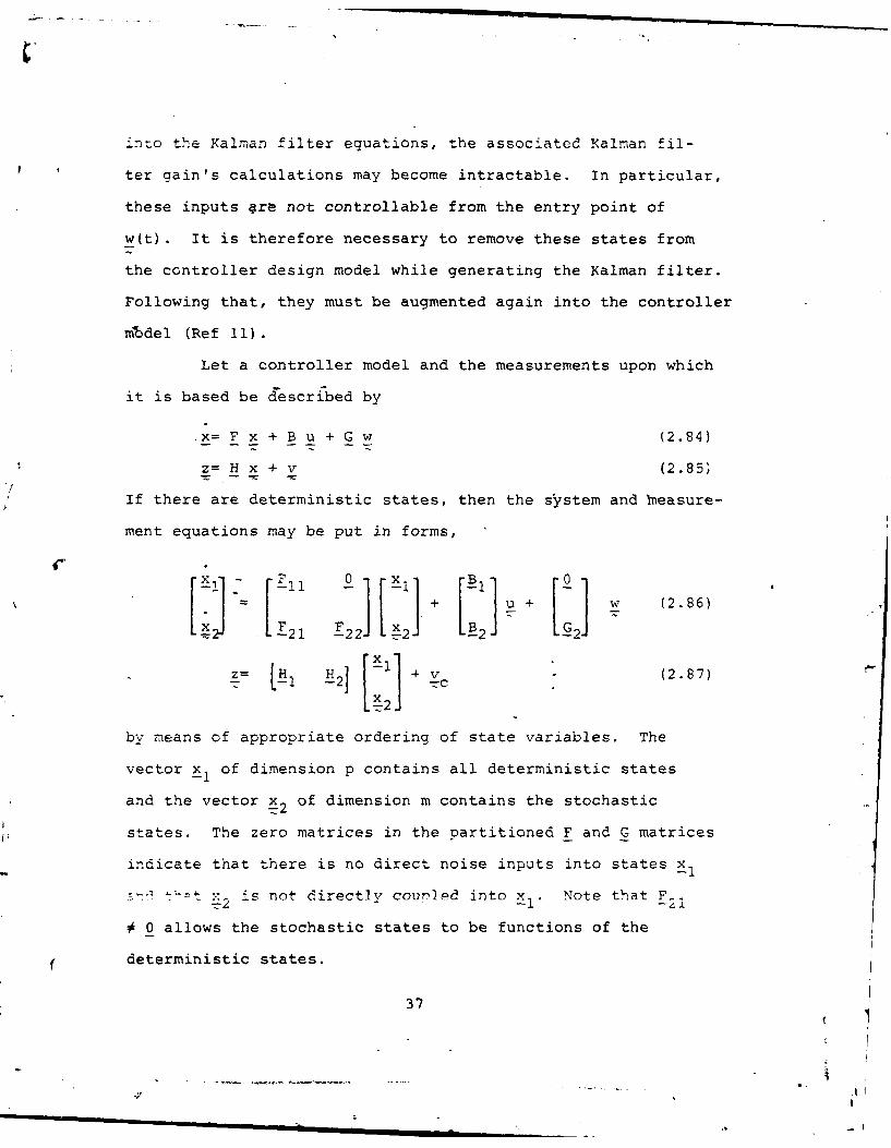
x= F x + B u + G w (2.84)

z= H x + v (2.85,

If there are deterministic states, then the system and 'measure-

ment equations may be put in forms,

+ w (2 .8 6 )

z= [1 i2 + v (2.87)

x2

by means of appropriate ordering of state variables. The

vector x of dimension p contains all deterministic states

and the vector x2 of dimension m contains the stochastic

states. The zero matrices in the partitioned F and G matrices

indicate that there is no direct noise inputs into states x

S X is not directlv courled into x1i Note that F_

# 0 allows the stochastic states to be functions of the

deterministic states.

37

Now to produce an estimate of x , 2' a Kalman filter,

for a system partitioned as in Eq(2.86), can be determined

using Eqs (2.2),through (2.13) so that

A

-2= -22 A2 F 21 -xl + B 2 u

. -H (2.88

Note, the Kalman equations require only the m by m F22 matrix

and the m by r G2 matrix (where r is the dimension of w) from

Eq (2.86) in order to compute The Kalman filter gains.

Once the Kalman filter gains Kf are determined, it is

necessary to reform the complete controller model as in

Eq (2.89)

'-X L _2 LE212 B-2

+ (z - (2.89;-fc

Now the controller will provide values for all controller

states: known values for the deterministic states and esti-

mates of the stochastic states.

Samrled-Data LQG Controller

The following discussion of the sampled-data LQG con-

troller is based on the presentation by Maybeck (ReflO). It

assumes that the underlying physical system to be controlled

can be represented by

38

4'

'4

x (t.) ±(ti I t i (ti + ka(ti) it )

+ d(ti') (ti) (2.90)

where i(ti+l t i ) is the state transition matrix and Bd(ti),

9d(ti) and w (ti ) are the discrete-time counterparts of B(t),

G(t) and w(t) described previously for continuous-time systems.

4ote, if the underlying physical system is a continuous-time

system as in Fig (2.5), then Eq (2.90) represents the equi-

valent discrete-time-representation of that system as opposed

to an approximate discrete-time representation (Ref 10).

A sampled-data controller for the system of Fig (2.5)

is an optimal controller in the sense that it minimizes J in

Eq (2.91)

Ej TtN+t f Z(tN+l)

N+ E 2 xT(t i ) 2i(t i ) 2 (t i ) + u (t i ) ii(t i ) 3a(t i )

+2 xT(t.) S(t i ) (t + J t i ) (2.91)-- i=O r

In Eq (2.91) Xf is the cost-weighting matrix for the final

state which occurs at the final time t N+1 , (ti ) is the cost-

weighting matrix for the states at time ti , U(t i ) is the cost-

weighting matrix for applying controls at time ti , S(t i) is

the cost-weighting matrix at time ti relating certain con-

trol values to certain states, and J r(ti ) is a residual cost.

Note that the applied control is held constant throughout

each interval between sample times and that no control is

applied at the final time, tN+1.

39

~(jKalman I

I One-sanmnle nemry.r

LQG Feedback Compensator

Fig 2.5 Sampled-Data IJQG Controller (Refl10)

V7hen 7Q (2.90) is an equivalent discrete-time repre-

serntation of~ a system, a complete characterization of the

states and cost can be generated by simultaneously integrating

the differential equations, Eq (2.92) through (2.98) forward

from. time -1-,o t, . (Note G.= I f~or su~ch a reireserntation).

~(t, t~ ) F(t) B(t, t i) + B (t) (2.93)

j(t, t> f(t) g(t, ti) + (t, +: Flt

40

-XX -UU

MSYi ) xu + u(t) B(t, ti , (2.96)

_§(t. t i): kT(t, ti ) W~xx(t)BF(t, ti)

+ T (t, ti ) Wxu(t) (2.97)

4_(t, t i): tr [Wlxx(t) Q_(t, t i ] (2.98)

Initial conditions for all integrations are 0, except for

!(ti, ti)= I. At the completion of the integration to ti+ 1 ,1.. 1t + - t +

t- desired results are t , > L d )=_9 , ti,

1 1 - -i+1 i) S (t)= T(t 1X(t i)= Z(ti+ I , t i), i_(ti)= ii(ti+ I , t i), S(t i)= S-(t i+1 , ti )

and J r(t.)= r (t i+, ti). The integration must be performed

for every sample period, except in the case of a time invar-

4iant system model with constant cost-weighting matrices and

stationary 1.oise inputs with fixed sampling period, where the

integrations need only be performed once. In this later case,

the i, Bd and G matrices in Eq (2.90) and the X, U and S

matrices in Eq (2.91) are constant matrices (Ref 10).

For a system described by Eq (2.90), the LQG regulator

consists of an optimal deterministic state feedback control-

ler cascaded with a sampled-data Kalman filter as in Fig (2.5).

The Kalman filter provides an estimate of the states. This

ccnditional mean estimate x(t) is descrited by Ea(s 2.99

through (2.99E).

-S2*(ti)= _ t ,ti i x +t _ ) + Bd(ti_j) uj(ti_ I ) (2.99A)

41

- - -- 2

P(t)= (t, t ) p(t T

+G d(t i_1 ) Qd (t i-l G d(t i_ (2.99B)

K(ti)= P(t.) HT (ti )

[H(ti) P(tH) HT(t) + R(ti)]- (2.99C)

xk(t+)= (t-) + K(t.) (t ni.. x (.(.91

+P(t+)= P(t l) -K(t.) H(t.) P(tT ) (2.99E)

The initial conditions necessary for beginning the recursions

indicated by Eqs (2.99A) through (2.99E) are the a priori

knowledge of : and P , that is,

o --O--(t )= p (2. 100A)

E 0o) -o P (2.100B

Qd(ti) in Eq (2.99B) represents the covariance of the assumed

zero mean input noise w (ti), that is,

E~~ (QT( d (ti) t.i= t.j*S-d (2.101)

0 t. t

z. in Eq (2.99D) is the measurement available at time t. and

is of the form

z(ti)= H(t i) x(t i) + v(t i ) (2.102)

where v(t.) is an assumed zero-mean measurement noise of

covariance R(t) , that is,

42

S (t t.

Note t -(t) va(t 0 r (.

Note that ](ti) and v(t i) are also assumed to be independent

of each other. The description of the various matrices and

vectors in Eqs (2.99) through (2.103) parallels the continu-

Qus-time case with the exception that there are now two

values for x and P. The value at ti is the value before the1

measurement at I., z4ti), is incorporated. The value at t+- 1 1

incorporates the new information made available by the mea-

surement at time t. (Ref10).

The optimal deterministic controller to be cascaded

with the Kalman filter in Fig (2.5) is described by

Su(ti) -(t i ) x(t i ) (2.104)

Eq (2.104) assumes perfect knowledge of x(t.) at the sample

time. Since the certainty equivalence principle applies,

x(t i ) can be replaced by _ (t+ ) when knowledge of x(t i) comes

from incomplete noise corrupte measurements. G*(t i) is,-c1

from deterministic QG controller theory (ReflO),

-c(t U(ti (t) K c(til)B(t

[(ti) +cTi c i+6 td(ti)

where K (ti ) satisfies the backward Riccati recursion-c 1

e~43

ii .'

K (t)= X(t+) + (ti+, i) c (ti+ i+l' Ti

L- 1 _Kc(ti+i !t i+, t i )

+ ST (ti)T G*(t i ) (2.106)

K (tN+1)= Xf (2.107)

Flowcharts and FORTRAN source code required to imple-

ment the sampled-data LQG controller appear in Appendices A

and B respectively.

Sampled-Data Performance Analysis

This performance analysis is based on.Fig (2.2), with

the only difference being that a sampled-data controller is

used versus a continuous-time measurement controller. This

performance-analysis scheme is from Vaybeck (Ref 10'.

In this scheme the truth model is represented by

x(t)= Ft(t) xt(t) + B (t) u1(t) + Gt A (t) (2.108)

and the measurements available to the controller are sampled-

data measurements of the form

zt(t. ) = Ht(t i' x (ti + v (t ) (2.109)Wt i t t i t~t

The discrete-time controller, which is similar in form

to Eq (2.23A) and (2.23B), is

ui(t) Gc(t i c(t ) + G c(t i ) zt

p+ G cy(t i ) yd(ti) (2.110A)

44

c ( )+ = Jc(t i+ , t i ) X (t i ) +Bc (t i

i+ B ( -z t i

+ Bcy( i I d j 2!-

The primary differences between Eqs (2.23.) and (2.110) are

that the differential equation is replaced by a difference

equation and that the counterpart to z4t) is written itias

opposed to zit i ) (Refl0).

Using a controller as described in Eq (2.110), and an

equivalent discrete-time model for the truth model, the sam-

pled-data performance analysis is very similar to the contin-

uous-time performance analysis where W (t) and ya(t) become

Xa (ti) and y(t.). That is, if in Eqs (2.27) through (2.35)

(t), X (t), t(t), xt(t) Fc(t). Ft(t), are replaced bywe c , t # ''

_(ti+) X(ti), xt(ti+,), xt(t i (ti+1, ti), _ t(ti+l, ti),

respectively. Then F (t) becomes &_(ti+, ti), 1_a(t) becomesa i+ -

Bda(t i ) and Ga(t) becomes Gd a(t.) where the upper left parti-

tion in G is the identity matrix I, since this is an equi--a

valent discrete-time representation. If the'underlying truth

model is a discrete-time system, an appropriate Gd would re-

place the I.

The mean mxa (ti ) and the covariance P xa(t) of the

internal process xa are propagated by

X (ti+l)= !-a(ti+1' ti)ix (t) + Bd (ti) (t(la a -a (2.111A

B4

.t )= (t) ' (ti T(ti , ti-x a 'i+l ti+l PX a 1 - 1+

+ 1 ( ( 'Tj z: ( i) (2.11 !B '--a d a --d a i

The mean and covariance of the augmented vector of desired

quantities, La, are given as a linear combination of the sta-

tistics of xa consistent with the definition of La (Refl0):

--ya G)_cz (t i H!t(t i) Gac x ti) mxat)

00

t)I (ti (2.112A)[cy ti )

P Yat) z( t H cx(ti Exa (t i )

- c~i 2 H (ti) G~ iL Z1-t1 c x

0 GT (t.)

[ I1- R(t.) 1o GT ()T (2.112B)

[ acz(ti)J - -z

Eqs (2.111) and (2.112) will give an accurate descrip-

tion of the desired statistics at the sampled times ti . How-

ever, it is often desired to know the statistics at particular

mcments between sample times. The differential equation for

0~~* xa( ) is

Ya u 0 0 u(t)wt rt)

(2.113)

46

. ,-

Based on Eq (2.113), the mean my(t) ad.. covariance F ('

are propagated between sample times by

[Ft(t) t (t)-a (t 001my a (t ) (.11A

P (t) -- t Q[ [ -)

0 !Lt) (t) P

-ya _o+Za ii; (t 0

[Gt~t) Qt(t)G T (t) 0

t 01 (2.114B)0 0

The initial conditions for the sample period beginning at

time ti, come from Eq (2.112). Note that no.Pxa vt(t.) terms

appear in Eq (2.112B) as they do in the continuous-time coun-

terpart, Eq (2.46). This is true when w (ti ) and xa(to) are

assumed independent of v t(t i ) (Ref 9).

The optimal LQG regulator must be put into the form

of Eq (2.110B) to be evaluated. The optimal IQG regulator

'has the control law

u*(t.)= -G*(t.) _(t.) (2.115)

w:ith 0d= 0 the necessary associations are, from Mlaybec'x: (Ref

10),

-cxt1 -c ti) - t i1

2 (t-CZ

47

k7, ( ti)= [L(ti+l, ti) - d(t.) Gc(ti +

• K(t i ) (2.119)

4 B = 0 (2.120)-cy -

qcy= (2.121)

where the ?, B , G* and the filter gain K are those associated-0 C

with the controller design model.

Since there are minor differences between this per-

formance analysis and the continuous-time performance anal-

ysis, only one software routine was written to accomplish

i bch of the e performance analyses. External flags set by

the calling routine indicate to the performance analysis

routine whether it is to perform a continuous-time or dis-

-crete-time performance analysis. Flowcharts'and FORTRAN

source code for the performance analysis appear in Appenices

A and B respectively.

Doyle and Stein Technique in Discrete-Time Systems - 1

This section describes the first approach taken in

this thesis to try to extend Doyle and Stein's (Ref 2) tech-

i fcr enhancing robustness of ccntinuous-time LQG con-

7rollers to sampled-data LQG controllers.

In this approach, the continuous-time LQG developed

48

iP

using Doyle and Stein's technique is merely discretized.

IThis discretized controller must be put into the

performance analysis format which requires values for G_cx (ti),

Gcz(ti ) and G cy(ti ) in Eq (2.110A) and I (ti+l, ti), Bcz(t i )

and B (ti) in Eq (2.110B). Since G*(t) is constant, G (t.)-cy 1 c -cx I

= -Gc where the control law has become u(t.)= -G* x (t.).-c - C -C 2

Gtz is zero and since yd= 0, so is G . Then for

the controller of Eq (2.23B)

2c(t)= F (t) Xc(t) + Bcz (t) zt(t) + Bcy(t) Yd(t) (2.23B)

xc (ti+l) in Eq (2.110B) becomes

+ [ cy(t ) At Y d(ti) (2.122)

.:here &t is.the sample time and I +(Fc(ti) At) , Bcz (t)At

and B (ti)At are first order discrete-time approximations-cy1

of --c (t.i, ti), B (t i ) and B (t i ) required in Eq (2.110B)

iRef 9). Also note that a discrete-time approximation of

R (t) is required. From Maybeck (Ref 9) an appropriate

approximation, R(ti.), is

R(ti)= R (t.) /At (2.123)- 1 c a.

Recall that cF Bcy and B are defined in Eqs (2.58)

through (2.60) and are described in terms of the continuous-

time controller model matrices, the Kalman filter gain (which

is calculated using Doyle and Stein's technique) and the

0 deterministic controller gain.

49

• m A

The Doyle and Stein Technique in Discrete-Time Systems - 2

( 0 This section describes the second approach taken in

this thesis to extend Doyle and Stein's (Ref 2) technique

for enhancing robustness of continuous-time LQG controllers

to sampled-data LQG controllers.

In this approach, a sampled-data LQG controller is

u-sed. In order to apply the Doyle and Stein technique,

2 T in Eq (2.99B) is replaced by 2A. In this controller,i -2d 2d -d

Q the assumed discrete dynamics input noise strength, is

related to Q(q) of Eq (2.64) and is

,_T q2 TBd- T B V B At (2.124)

Eq (2.124) is a format similar to using G Q dT of the dontin-

uous-time system multiplied by At as d first order approxi-

mation to Qd (Ref 9). At is the sample period of the sampled-

data controller. Note that the subscript c in Eq (2.124) is

to indicate that the B matrix is the continuous-time model

B matrix.

Flowcharts and FORTRAN source code for the software

necessary to implement this approach appear in Appendices

A and B respectively.

Enhancing Robustness of Discrete-Time Systems by Directly

Choosing K

The third approach to enhancing robustness of sampled-

data controllers involves directly picking the Kalman filter

gain K. This approach is related to that of Doyle and Stein

50

_ _ _ _ __._ _ _ _ L

for continuous-time systems in> that a similar strategy of

making the return difference mappings for a full-state feed-

back system and an observer-based system asymptotically equal

is used. Fig (2.6a) shows the full-state feedback system

while Fig (2.6b) shows the observer-based suboptimal control

law configuration where u(ti)= -G (t-) instead of the opti-

mal control law where u*(ti)= G* (ti)" Note that the label-

ing in Fig (2.6) indicates that this analysis is done in the

z-domain versus.the s-domain for continuous-time systems

(Ref 10).

The return difference of the full-state feedback and

the observer-based design need to be equal in order for the

observer-based design to recover the robustness properties

of the full-state feedback controller. That is, [i KI is to

* be found such that

* K [ + H (z I 4)_ - 1 -

_-d ( (z I - -) Bd - ( .1 5)

Note that K is the steady-state Kalman filter gain and i is

the state transition matrix. If K(q), parameterized as a

function the scalar q as in the continuous-time case, is

selected such that

Lim 0 B ' (2.126)q

for any nonsingular m x m W then Eq (2.126) is satisfied

asymptotically. K is thus chosen as 4

51• , ...... t :Z " '-_. -T " ' ,

... *" ......... . .. .. -:: - _, - ---- '- .. ....... ... ...

(a)

+ +_

(b)

Fig 2.6 (a) Full-state feedback (b) Suboptimal control lawI u~3(ti = _- 9,(t.-) (Ref 10)

K= q 1 1 LC (2.127)

Now, q and WC can be varied as in the continuous-time case to

achieve the desired degree of robustness. Note, in the dis-

crete-time case, R is chosen directly, as opposed to choosing

a ..'-' In -e contiruous-time case (Eq (2.64) and then cal-

culating a K based upon the solution to the matrix Riccati

Eq (2.13) (Ref 10).

IYaybeck (Ref 10) indicates there are many possible

0 choices of W in Eq (2.127) above but that one particular

52

-,- --

choice is motivated by considering the dual state equations.

'I This choice, Eq (2.128),

w= B d) (2.128)

assigns m eigenvalues of the closed loop system to the origin

and the remaining (n - m) eigenvalues to the invariant zeros

df the system for a system of n states and m inputs.

In order to use the performance analysis algorithm,

the suboptimal 6ontrol law must be put into the proper format.

The proper format, from Maybeck (Ref ID), is

Gcx(ti ) = -G (t i ) (2.129A)

,cti1 ti)= k(ti+, t i ) JI - Kyt i ) Hi(ti)]

-cx i -c i1- -

- Y(ti) -*(ti) (2.129B)

Bc (ti)= _(ti+I t i ) K(t i ) (2.129C)

G cz(ti)= B cy(ti)= G cy(ti)= O (2.129D)

wheret t) Bd(ti) G*(t.) and the Kalman filter gain1~ -d ti -c

K(t.) are those associated with the controller model.

Flowcharts and FORTRAN source code for the software

necessary to accomplish this choice of W and to vary the

parameter q appear in Appendices A and B respectively.

53

I.!

III Results and Conclusions

IIntroauiction

This chapter discusses the results and conclusions of

this study, based on data generated by the interactive computer

program written to support this study (see Appendices A

tnrough E for program description). There are several items

about the following discussion that need to be addressed at

this point. First, the following discussion of the various

controllers and performance enhancement techniques includes

data obtained for the software verification models (Test

Cases 1, 2 and 3) that are introduced in Appendix D. Second,

the Apollo model state vector was rearranged to meet the

software requirements for handling the deterministic state

(see Deterministic State Augmentation Section of Chapter II).

In this rearrangement the original states 1, 2, 3, 4, and 5

become states 2, 3, 4, 5, and 1 respectively, that is

T T= - (3.1)

Third, when discussing the results obtained for the Apollo

model only states 1 and 4 (6 and vb) will be used to demonstrate

performance since the behavior of states 2 and 3 is similar

to that of state I and state 5's behavior closely resembles

that of state 4, which is the state most direclty affected

by changes in " Fourth, even though the time histories of

the mean and covariance of the states and controls form the

q primary basis on which to judge closed-loop system performance,

54 1

the eigenvalues of each closed-loop system are computed and

9 examined to determine stability (prior to running the mean

and covariance analysis). Last, the matrix design parameters

V and W in the two performance enhancement techniques are

always 1-by-i matrices for the applications considered. They

are thus always set to 1 since any desired change can be

atcomplished by adjusting the appropriate scalar design

parameters. The order of the discussion is continuous-time

controllers fir!t, discretized continuous-time controllers

second, sampled-data controllers third and finally remarks

about some general trends applicable to all three-controller

types.

4P Continuous-Time Controllers

The steady state performance of the continuous-time

controllers without first applying the Doyle and Stein

technique for the three software verification test cases is

presented in Table D.2, Appendix D. The steaay state

performance of the controller for the Apollo model is displayed2

in Figs 3.1 and 3.2 for wb of the truth model set at 100 and

400, respectively (wb in the controller design model is set

at 100 for all cases). Figs F.1 through F.3 of Appendix F

show Apollo model performance for several other values of

2b' Note from these Figs that the closed-loop Apollo system

is unstable for 2 < 50 and 2 > 400 (evident in state 4b - bh.

only for this last case).

55

E0

a,

- UP

to 0

0 0

L) 0

E --

to- 0t - IS-- sz0 ST0 a so oo d' \*

tlxu

S404

0d )

db. 0

I N U)8 I-

56

W 4-)

U) 0

0

Q) Cd0) 94

M 00

0

- .4-4

00v 0

co

0

-404- 0

4. CD --' )

4 0)

0(z .)

30 100 o * to& 00-0 so0 10 ;o oOv'

,.O1.w I±X I.0

57

'1

When the Doyle and Stein technique is applied to Test

Cases 1, 2, and 3, the performance is improved in the sense

that the density functions are more tightly packed around the2

mean values (state estimates known more precisely) as q

(the Doyle and Stein scalar design parameter) becomes large;

see Table 3.1. This is indicated by the fact that surfaces

of constant likelihood, planar ellipses in the two-dimensional

2case, contain less area as q increase where the area is

directly proportional to the product of the eigenvalues of the

steady-state covariance matrix, P (Ref 9). (A quick check,

applicable in the two dimensional case, is to conpute the

value of P11 P2 2 - P1 2 since this value is the magnitude of

the two eigenvalues of P multiplied together. Note, in all2

cases presented here, the P1 2 is a negligible term and thus

only values-for P11 and P22 are given in the tables that

follow.) By examining Table 3.1, Doyle and Stein's claim

that their method moves some of the filter poles toward stable-~ 2

plant zeros and the rest to - (asymptotically as q becomes

larger) can be verified.

Note that the Apollo model used in Table 3.1 includes a

damping factor, , of 0.001 in the bending mode dynamics

(i.e., the 3, 3 term in the F matrix of Eq (2.75) is no longer

0 but becomes -2b. A damping factor was added because no

noticeable performance improvement could be obtained with

0 (which places a set of poles for the bending mode dynamics

on the imaginary axis) and it was anticipated that moving the

58

A .

-, m m

CN N N

+1 +1 +!

0 0 0 0~K 0 00 0

04c 0 0 -4cqI.

0. en q M- ko N J'4 *m 1m r 0 0 1+1

-W +1 + -4 .. w

r ..- Oa 0 C D R r c o 0 0 r : 0j *v v. - ' 40Lnm '0 Q %D 0 0 0 *% -4 0*- H 0-4 m' N N %4 '0 C-4 - N- r-I T-4 M ~ '. -4 en 4

CQ. Q DW04 en I I II I I I

ZE4-I Nr,

4 0

*LwC 4.) I n

0 1 4-1 m.I) 41 0 0

m ~ " r'I - 1.oj M A N Nf-E-0r - 0. '. '. - n

fu) m ) * 0) m~ %D c-4 '.0

04 4.1 En A ~ N 4 ,

0 1 ~LA U' - - - .*. %D-

nj~O N 'o0 r .0 1 1 N N m 1-1.4- N- N- LA) ' 'Rr N N N m'1-

V4.1-) .1 . -4 -. -4 .4 Q 0 0 ('

V) COI 0 0 0

>1"r r4 r

CN - 000 a 0 -4 000-q- 0 0 04 ~0 00 0 Oj 0 0D

-4 0 *-4 01-4-4 -4-4 4

C).

U 0 0 0$ -4 -- -f -q

M0o -4 -4 -41 -4 - 'N N CN m m~ m m 0 '0a) 0

59

0) 0 0 0C) 'r-4

4-) 0CA w 0 0 0 0 lN 0

u oU.Z4-)

(N (N CD 0 4-4 Q) 41CD 0 m' -4 00 4 M

*4-4 41 C) rI r- It (N (N .,4vI

z -- 1 04-4~ 34 P. a N - 0 ~~

) (N 0 '-q 0 0CD1

' ~ c r-044 4' C '*-I

4404N C) Q -441 q 4.0

0 -) C

o~L (N4 (n0~- (

-4 ~ ~ . (N C41J4 C) r

1~~~> U 0~ )~~).)Cr4) 4-) I C)

)4- U) U

>1 0 1N N C) It O r. w

-.1 r. W -4 ) 4 a ) m

(N 'iQ)4 -w 0 - u

en~C N Lo rd U) 14-i a)C C) 'C)1 1

E-L) C - 4 - Cb)

41 C40 ) (C) -

-1 0n N -4 0 (N -r' .- I U-4L E -4(N 4I.

0.4. 41 W .w.C

C) C C) 11NC) I C 4.) C)

C) N -4 U ) 0 )C) r-. - n C)C a)4 (N

4-0C .0 . 0 .0 .1 .0 0 .0 0 C 0 uU) 0 -0 '1 0 M I C~ 0

Q) -l Q

60u

poles away from the imaginary axis might allow the Doyle and

Stein technique some extra "maneuvering room" in which to

bring about stehdy state performance improvement. Several

damping factors between 0.001 and 0.15 were tried to see if

steady state performance could be improved but no noticeable

improvement was obtained for any value tried. (No values

)arger than 0.15 were tried since C= 0.15 is already 10 times

larger than that in the actual Apollo system.)

Table 3.1 shows only marginal improvements in closed-loop

stability for the Apollo model as q increases until some

critical value is reached (approximately, q2= (701)2) at which

closed-loop stability is lost. Note that one of the filter

poles is positive for q2 < (701)2, the stable closed-loop

system case, and that the filter poles do not migrate as Doyle

S2 2and Stein suggest but abruptly, at q > (7 0 1 ) , change to the

configuration where some are co-located with system zeros and

the rest have larger negative real parts. At this point

closed-loop system stability is lost. It is~noted that in the

case of the Apollo model, the Doyle and Stein techniques adds

white noise in the system before the first order lag (where

noise did not previously enter) instead of after it and this

may affect the resulting performance of this technique. This

phenomenon should be investigated further.

Table 3.2 presents the results for Test Cases 2 and 3

when the strength of the continuous-time noise Q is "tuned"

by adding a LQ which is a simple scalar multiple of Q. AQ is

61

,. - . .. , . .. . , & .. ... . . . .

fTable 3.2Steady-State Performance of

Continuous-Time Controllers with'Tuningof Q by Adding A0

Test Q, 4Q Steady-State FilterGase PT P Poles

-5__ tt uu

2 10, 1 4.4(10) , 6.1(10)- 2.3 -9.6±j9.1

2 10, 100 2.9(10) - 5 , 5.0(10 - 3 5.0 -40±j40

2 10, 1000 1.9(10) - 5 , 4.7(10) -3 79.6 -125±j125

3 1, .1 219 , 2091 4..3(10) 4 -7.25±jl.7

3 1, 1 210 , 2229 6.5(10) 4 -11.3, -6.6

3 1, 100 179 , 2784 6.7(10) -90, -5.9

3 1, 1000 173 , 2914 7(10)6 -9000, -5.8

3b 1, 10 o c -28.0, -5.99

3b 1, 10000 o c -900, -5.90

3b 1, (10) 6 M 0 -9000, -5.90

a) Only diagonal terms Pill P 2 2 shown.

b) Truth model F matrix deliberately mismatched with controllerdesign model; Ft2 = -100. Test Case 2 not shown; it alsot,2

could not be stabilized using this tuning procedure.

62 j

chosen such that it approximates the value of noise added by

the Doyle and Stein method. Tuning Q in this manner adds noise

at the pointsoT entry of w into the system dynamics instead

of at the point where u enters as in the Doyle and Stein

technique. (Test Case I is not displayed because there is no

physical difference between the Doyle and Stein technique

And this tuning procedure for this case.) Comparing the results

for Test Cases 2 and 3 shows that there is not much improvement

from one method to the other for Test Case 2, but that there

is a noticeable difference for Test Case 3. Note, when the

closed-loop system of Test Case 2 was made unstable (by

changing entries for the F matrix) in order to show robustness

effects, that neither procedure (Doyle and Stein or adding AQ)

- could re-stabilize the closed-loop system. For Test Case 3,

the Doyle and Stein technique gives better results in the sense

that the surfaces of constant likelihood, contain less area

indicating that density functions are more tightly packed around

the mean values. This approach was not appl.ed to the Apollo

model since the results of the Doyle and Stein appruach were

poor.

As far as the Test Cases are concerned, the Doyle and Stein

technique appears to be a valid approach to improving the

performance of continuous-time systems even for values of q

less than . For Test Case 3 this technique is superior to

tuning the Q matrix by adding a AQ as a simple scalar multiple

of 0. In this case, the tuning procedure adds noise in both

63Ott ,4

state equations, but the Doyle and Stein technique adds noise

only to the second state equation, where the control input

exists. In contrast, either procedure adds noise at the

control input for Test Case 2 due to configuration of the

B and G matrices in the test case. As for the more complex

Apollo model, the results are inconclusive. While some

mrtrginal improvement could be seen for large q2 and w2= 400,

the total behavior of the system was not as expected. In

particular, thebehav ior of the filter poles, as discussed

previously, was not expected, especially since when the poles

were in the desired positions, closed-loop stability was lost.

Discretized Continuous-Time Controller

_The results of discretizing each controller without first

applying thF Doyle and Stein technique are presented in Table

D.2 of Appendix D. Examination of the entries in this table

reveal that the discretization process gives better results

for smaller sample periods, as expected since the first order

approximations used are valid for small (relative to charac-

teristic times of the basic system) sample periods (see the

Doyle and Stein Technique in Discrete-Time Systems - 1 in

SChapter II). Sample periods chosen for the robust versions

of these controllers were those for which the unmodified

controllers had essentially the same steady-state performance

as their continuous-time counterparts. Table 3.3 presents the

results for the discretized controlleis for Test Cases 1, 2,

64 Ai

- - *|

, Table 3.3

Steady-State Performance ofDiscretized Robust Controllers

Test 2 b Steady StateCase At q Pxtx a Puu

1 .01 1 1.78 .120

1 .01 10000 1.48 12.4

1 .01 (500)2 1.47 194

1 .01 (1000)2 O cc

2 .001 100 2.01(10)-5, 4.79(10) 71.5

2 .001 (25)2 1.86(10)- S, 5.55(10)- 3 305

2 .001. (49)2 1.77(10) - 5 , 6.78(10) - 3 953

2 .001 (50)2 -

3 .001 1 221 , 2122" 4.7(10)4

3 .001 100 235 , 1814 2.9(10) 4

3 .001 (100)2 316 , 1192 7.3(10) 4

3 .001 (1000) 2 CD

54

65"4

Table 3.3 (Cont)

Test 2 Steady-StateCase t q b P a P"x t xt uu

1c .001 0 00 00

Ic .001 1 00 00

1 .001 100 12.0 2.44

1c .001 (1000)2 7.33 128

3 .001 0 00

3 c .001 (1.,0 00

3c .001 10000 1025, 554 4.99(10)6

3 c .001 (1000)2 1533, 262 2.16(10)6

a) only diagonal terms Pill P2 2 shown.

b) q2 is the Dcyle and Stein scalar design parameter.

c) F matrices changed in truth model description to showrobustness. For Test Case 1, Ft = 0.1; for Test Case 3F = -100. Test Case 2 could not be stabilized once a

2 ,2destabilizing F was chosen.

66

I '

and 3 when the Doyle and Stein technique is applied. Comparing

the results for Test Cases 1, 2, and 3 shown in Table D.2 and

3.3 shows that Ziscretizing a continuous-time controller to

which the Doyle and Stein technique has been applied produces a

discrete-time controller with enhanced performance up to a

certain value of q

The Apollo model presented difficulties in this case

also. In fact, no matter how small the sample time was made

(periods down to 0.001 sec were investigated), the resulting

closed-loop system was unstable indicating that the first

order approximations were invalid. To improve the situation,

a damping factor was again added in bending mode dynamics as

in the continuous-time case. The initial choise of C= 0.015

and sample periods <0.01 sec allowed the resulting discretized

2continuous-time controllers to remain stable even though wb

was varied passed 400 which was the desired value about which

to investigate performance. By trial and error and noticing

trends in the data (the interactive computerprogram was well

suited to this task) a suitable combination of sample period and

damping ratio was found. With a = 0.01 and sample period

of 0.01 sec, a discretized continuous-time controller that

was initially unstable at wb= 400 could be made stable by

applying the Doyle and Stein technique before discretizing.

Values of q2 between (100)2 and (0.001)2 were tried and2= (00) 2

q (0.02 selected as the value that gave the best performance.

In fact stable closed-loop operation occurs only for

67

A

2 2 2(0.005) < q < (0.05) The fact that there is an upper

limit on the value for q2 is an aspect that is not seen in

the continuous-time case. Fig 3.3 shows the performance of

the unstable unmodified discretized continuous-tine controller.

Figs 3.4 and 3.5a show the performance of the discretized

controller after the Doyle and Stein technique is applied

2= (012 2 2where q (0.1) For q = (0.02) the results are shown in

Figs 3.5b and 3.6. It is quite evident from these Figs that

applying the Doyle and Stein technique can cause dramatic

improvements in performance.

Thus, applying the Doyle and Stein to a continuous-

time controller and then discretizing the res.ult to produce

a robust discrete-time controller, appears to be one acceptable

approach to extending the Doyle and Stein technique to discrete-

time controllers. Note however, that since the discretization

process requires appropriately small sample-times, it is

anticipated that there will be some cases where this technicue

cannot be applied readily. The Apollo model is a good example

of this since in the actual Apollo system the sample period

is 0.1 secs which is 10 times slower than that which produces

a stable closed-loop system. One other item to note at this

point is that the interactive computer program is well suited

to any tuning (trial and error) that may be required. In fact,

the author accomplished the tuning described above in several

hours of interactive computer-time, whereas it probably wculd

have taken several days using batch processing.

68

-- _--

damping ratio= 0.01

0

0"-'.0O0 14.29 28.57 42.86 57.14 71.43 55.71 2G0. 00

secs

a) variance of state 1

damping ratio= 0.01,-tDbC-

0.-', 00 14.29 2i.57 42.86 57.14 71.43 35.71 100.00

secs

b) variance of state 4

Fig 3.3 Discretized continuous-time performance.with Jb=400 inthe Apollo model.

69

-4

CL) a

.C)Cd

aaCCD

r, CDj

c) I

C).Er

* *z

*Olm ~tm 5-

00

Cd)

91 -a so; s d-oS;Gi si &

700

CO.

C,,

S 14.29 2i.57 42.85 67.14 71.43 B5.71 100.00

secs

a) control variance when q2 =0.01

9,o.

0

CO,

I

0.0 - 14.29 2i.57 42.86 S7.14 71.43 85.71 100.00

secs

b) control variance when q2 =0.0004

Fig 3. 5 Discretized continuous-time performance with 2=400

and q2=o.01 and o.0004 (control variance)

71

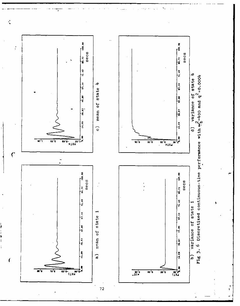
CC

CDC

4- 0

CD .)0 r- )

z U d

cda 0

CgCd

0o C )

4-

CCr.-

C)0

Cd

CD 0 4-)

U' 0)

I. -A

0! C)Cd \)

r bD

WO ' 100 *£0- .*0 0.0 to0 30 0 co~f1.1 XW li±x~

72

Sampled-Data Controllers

This section presents the results and conclusions

concerning the performance of the robust sampled-data controllers

developed in this thesis. A discussion in the effect of

applying the Doyle and Stein technique (as extended in the

Enhancing Robustness of Discrete-Time Controllers - 2 section

(;f Chapter II) appears first, followed by comparison with the

effects of tuning the Q matrix (by adding a LQ as in the

continuous-time discussion). Last there is a discussion of

the results for picking the Kalman filter gairZ, directly

(see appropriate section of Chapter II).

Doyle and Stein Techniques Extended to Sampled-Data

Controllers. The steady-state performance of the sampled-

data controllers for Test Cases 1, 2, and 3, with no robustness

enhancement, is shown in Table D.3 of Appendix D. Note here

that, as for discretized continuous-time controllers, the

sample period can greatly affect the steady-state performance.

The performance of the sampled-data controller for the Apollo

model, with no robustness enhancement and for several different

2.values of w, is presented in Figs 3.7 and 3.8 and Figs F.4

through F.6 of Appendix F. As in the continuous-time case,2b < 50 (although thisthe closed-looo system is unstable for wb 2--0(atoghti

is not shown in the above Figs). In the sampled-data case

2instability also occurs when wb > 200. (Note 0.1 secs is the

chosen sample period for the Apollo model since this value

gives good performance and is the same as that used in the

actual Apollo controller).

73

-I.,. I

00

W W

4-)

+) 0

4-;' 0to 0

a) -

g 0

Cd

o 0

0 -0

0ix C.) C

C

aa

94~

co a)

3 +B

4z

4,0

4--l 0

4--l 0

to

C P4

E>=

0 E

LZ~w Lo 10 (1) S IT U O ~ N.

10

4-1 ~C.)

0 r0Ld

Cd~

so 0 Zoa 3*-9*-2. o MD o~

.1x I 0x~

05

The steady state closed-loop performance with the Doyle

and Stein technique applied is presented in Table 3.4 for Test

Cases 1, 2, and- 3 and in Figs 3.9, 3.10, and F.7 through F.10

for the Apollo model. Comparison of the results presented in

Tables 3.3 and 3.4 shows, for Test Cases 1, 2, and 3, that the

steady state performance is enhanced as q 2 increases in the

sense that areas of the ellipse representing the surfaces of

constant likelihood become smaller (see related discussion of

these surfaces 3Tn the Continuous-Time Controller section of this

chapter). For the Apollo model the results are similar. Figs

3.9 and 3.10 show stable closed-loop operation for w= 400

Pand 700, respectively, while Figs 3.7, 3.8 and F.6 indicate

that the closed-loop system with an unmodified controller is

22unstable for Wb > 300. By examining Figs 3.9, F.7 and F.8,

one can see-that there is a value of q2 (in this case between

(0.1) 2 and 1.0) beyond which increases in q2 produce no

noticeable difference.

, As in the continuous-time case, a compaeison is made

between the Doyle and Stein technique benefits and those benefits

obtained by tuning the Q matrix by adding a scalar multiple

of Q, LQ. Also as in the continuous-time case AQ is chosen so

as to approximate values of q used. When this technique is

applied to Test Cases 1, 2, and 3, the performance could be

made similar to that obtained by applying the Doyle and Stein

technique as shown by comparing the results in Tables 3.4 and

3.5. In contrast, Figs 3.11 and 3.12 show the performance

76

Table 3.4

Steady-State Performance ofSampled-Data Controllers with Doyle and

Stein Technique Applied

Test 2 b Steady StateCase At q P xtxt a Puu

1 .01 .a 1.79 .105

1 .01 1 1.78 .119

1 .01 100 1.58 .900

i 1 .01 (1000) 1.46 61.5

2 .01 .01 4.00(10) .5 6.0(10) .3 2.28

2 .01 1 2.70(10) -5 5.1(10) - 5.11

-5 -2 .01- 100 1.75(10) - , 5.4(10) - 51.8

-5 32 .01 10000 1.65(10) , 6.4(10) 110

.2 .01 (1000)2 1.65(10) - 5 , 6.4(10) - 3 113

3 .01 .01 341 , 1108 655

3 .01 1 341 , 1108 652

3 .01 100 349 , 1078 473

3 .01 10000 316 , 1193 774

.77

Table 3.4 (Cont)

Test q2 b Steady-StateCase At qP x ta P U

44 1c .01 00 C

1Ic .01 1 c

I c .01 100 12.0 2.43

1c .01 (1000)2 7.35 63.0

3c .01 0 c

3 c .01 100 mo

3 .01 (100)2 996, 551 4.96(10)6

3c .0-1 (1000) 2 1554, 257 2.03(10) 6

a) only the diagonal terms Pill P22 are shown

b) q2 is the Doyle and Stein scalar design parameter

c) F matrices changed in truth model descriptions to showrobustness. For Test Case 1, F.= . for Test Case 3,F = -100. Test Case 2 choul not be stabilized oncet ,2a destabilizing F was chosen.

78

EO toW

~~4)

I-4-4

cd 0

to (D

)-4

0)0

C, 1 0

0SB*0 00 4--4- ~0 CO ?0 0

4

0)

c; 00 69- o c; LE0 W 00 OISDx I 0~

79 o

.04 1,

.40:p .0 .0

00.

a) C

lz ~ ~~ ~~~ vs0slo t oo D t

U))

S12? 6O 90- S1~SCO 00 00 Od ~ E

0

C. EU)d

0 r- 0

> 0D

Kjx .Di I M

0

Table 3.5

Steady-State Performance of Sampled-DataControllers When Q is Tuned by Adding AQ

Test Steady-StateCase At Q , Q Ptxt a P uu

1 .01 2 , 1 1.73 .156

1 .01 2 , 100 1.53 1.97

-5 -32 .01 10, 1 3.92(10) 5.69(10) 2.68

2 .01 10, 100 2.52(10) -5 5.02 (,10)-3 6.22

2 .01 10, (10) 4 1.67(10) 5 , 5.90(10) -3 80.3

6 -5 -32 .01 10, (10) 1.56(10) , 8.47(10) 231

3 .01 1 , .1 340 , 1110 672

3 .01 1 , 1 337 , 1122 782

3 .01 1 , 100 325 , 1163 2390

43 .01 1 , (10)6 324 , 1169 4800

3 .01 , (10) 323 , 116949

81

I

Table 3.5 (Cont)

Test Steady-StateCase At Q , AQ P a P

x txt uu

i b .01 2, 0 00

ib .01 2, 1 Largec Largec

Ib .01 2, 100 9.33 3.43

01 - 2S .01 2, (1000)2 7.34 72.1

3b .01 1, 0 00 00

3b .01 1, 100 00

3b .01 1, (10) 4 00 00

3b .01 1, (10)8 00 00

a) only the diagonal terms P 1 1 P22 are shown

b) F matrices changed in truth model descriptions to showrobustness. For Test Case 1, F = .1; for Test Case 3F t = -100. Test Case 2 not shown, but it could not

2

be stabilized using this technique once a destabilizingF matrix was chosen.

c) Steady-state not rached during length of simulation,but eigenvalues are within the unit circle.

82

-40

0 0 004-'

00 9

N Pd

caa

QN Pd)

o 0

CO. 4. :

to a)

0 1

CsJ,

a a%

sol ao21- c 0.sl 00h.Di aiw'0 x1I

0 La83

C,)

00co0)

C4 cd

0 0

04 '

0)C. N C

-CS

> >

DS Z to I tgo 0 Os Z LS T soI od

C\I'

au, 0 MEC. 0 o C0)

01o

Or 0i 0)

a. 4,- UV

m C)

4-:'. cu

0 0~

Cd cu

84

of the Apollo system when the Q and LQ tuning procedure is

used. Note only the mean of state I and variance of state 4

are shown but al states exhibit similar behavior. Note, from

Figs 3.11 and 3.12, that no matter what value of AQ was added,

there was lirtle or no orforarce benefit. While the largest

AQ shown in Figs 3.11 and 3.12 is 10,000, larger values were

tried but the closed loop system eigenvalues rapidly moved

outside and away from the unit circle resulting in even more

unstable closed7loop-operation.

Based on the above comparisons and discussion, the

extension of the Doyle and Stein technique to sampled-data

systems provides a valuable tool for performance enhancement

in the face of uncertain parameters in the controller design2

model. For the Apollo model, values of q as small as 0.0001

effectively created a stable closed-loop system as shown in2

Fig F-9. (For q > 0.01 the increase in stability appears more

dramatic at first glance, Figs 3.10 and F.9, but this is partly

due to a much larger initial transient that o ccurs when q2

increases.) Tuning 2, by adding a zQ, that is a scalar

multiple of Q, had little effect on the Apollo model since

this did not add additional noise at the control input as the

Doyle and Stein technique did.

Robustness Enhancement by Directly Picking K. In

general the results from this tezhnicue were unsatisfactory.

For Test Case 2 and the Apollo model, there were no combinations

of the scalar design parameter q (see the applicable section of

85

AD-AI1S 478 AIR FORCE INST OF TECH WRIGNT-PATTERSON AF9 ON SCHOO--ETC FIG 1/3ROBUST CONTROL STSTEMS.1U)DEC 81 E 0 LLOYD

UNCLASSIFIED AFIT/GE/EE/810-36

2,

NOEomliii I "

Chapter II) and sample period that produced stable closed-

loop systems. The results for Test Cases 1 and 3 are presented

in Table D.3 ofr Appendix D. Test Case 1 is the only case used

in this study for which this technique provided performance

enhancement. For Test Case 3, using the areas of the ellipsoids

representing the surfaces of constant likelihood as the basis

of comparison, shows that the performance actually degraded

with increasing q. (Recall that the product of P11 and P22 as

given in Table D.3 is directly related to these areas.)

One possible cause for the failure of this technique

to produce stable closed-loop systems is that the suboptimal

control law u(ti)= -G* x(t.) was chosen as the basis of the

controller instead of the optimal control law u(t.) = -G* x(tt).1 -c- .

The case for the optimal control law should be investigated.

Another posEibility is that there is an as yet undetected

error in software used to implement this controller despite

thorough testing and validation. In any event it is noted at

this point that there are no stability guarantees for this

method of choosing K as there are for the LQG controller when

K is obtained as a result of solving the appropriate matrix

Riccati equation (Eq C.18 of Appendix C for example).

Remarks

Closed-loop system eigenvalues were determined for each

control system designed and were the primary basis of claims

about closed-loop stability. Although these eigenvalues indicate

8* 86

' ' " ,. . o. . .. . . .. 3 .. .. ..... .

stability, they do not directly provide performance charac-

eristics versus time of each controlled system. This

information is obtained from the mean and covariance analyses

developed in Chapter II. Both performance measures have

been presented here to provide an adequate portrayal of system

characteristics.

Another item of a general nature and applicable to all

the modified controllers, whether continuous or discrete-time,

is that as the noise level is artifically increased in the

system (via Doyle and Stein technique or by tuning Q by adding

LQ) the control variable variance generally increases (implying

increased control costs are incurred for increased robustness,

which is not surprising) . This fact should be considered in

any design attempting to apply the techniques for enhancing

robustness +hat are discussed in this thesis.

One final note involves the performance of Test Case 2.

This system did not behave "nicely" during the course of this

investigation. It could not be made stable when picking the

Kalman filter gain directly and it could not be stabilized

(using either of the two procedures tried here) once the F

matrix was changed to destabilize the closed-loop system for

robustness studies. The performance of this Test Case should

be investigated further and characterized.

87

IV Recommendations

The recommendations fall into two main categories. The

first deals with the basic nature of robust control systems

and the second deals primarily with increasing the utility of

the interactive computer program developed to support this

study.

Basic Investigation -

The first item that requires further investigation

and explanation is the fact that the Doyle and Stein technique

did not provide noticeable performance enhancement for.the

continuous-time Apollo system. There.are two aspects about

this particular model that may have affected the results. The

first is that there is no damping in the bending mode dynamics,

which places a pair of poles on the imaginary axis. An

attempt to allow the Doyle and Stein technique more "maneuvering

room" by moving these poles off the imaginary axis (non-zero

damping factor) was tried but was not successful. The second

is that for the unmodified continuous-time controller, noise

enters only states 2 through 5 but when the Doyle and Stein

technique is used, noise now enters before the first order

deterministic lag and thus into all 5 states. The effects of

this aspect on the Doyle and Stein technique need to be

characterized.

A second item is that, for Test Case 3, one of the

LQG controller poles (eigenvalues of F - B G* - K H)

88

is positive but the closed-loop poles are all negative and

thus the closed-loop system is stable. This phenomenon has

been observed.btfore by C.D. Johnson ("State-variable Design

Methods May Produce Unstable Feedback Controllers", Inter-

national Journal of Control, 1979, Vol 29, No. 4, 607-619)

and should be investigated and characterized. Another phenomenon

that should be investigated is the fact that there are upper

limiting values on q2 (in the Doyle and Stein technique) beyond

which the discretized continuous-time and sampled-data controllers

no longer cause closed-loop system stability, something not

observed for the purely continuous-time case.

The results for picking K directly were unsatisfactory

and this approach whould be investigated further. The

investigation should include the possibility of using the optimal

control law~u(ti)= -G* x(tt) as the basis of the formulation.- C 1

As mentioned previously, there are no guarantees of closed-

loop stability (even with no mismatch between the design and

truth models) when this method is used, unlike the case of

using the optimal gains from LQG controller synthesis methods

(when there is no mismatch of design and truth models).

For the cases where good results were obtained, exten-

sions should be attempted. The possibility of adding time-

correlated noise in a fashion similar to that of Doyle and Stein's

technique for adding white noise should be investigated. The

results would have potential applications in cases where the

noise process is known to be frequency limited. Thus the

controller would only expend extra control energy over a

89

2_

specific frequency band,:idth to achieve robustness instead of

over the entire frequency spectrum as is the case for white noise.

In addition, the results of extending these techniques to a

more general purpose controller, (as opposed to the simple

regulator used here) suzh as a Command Tracker Generator/

Proportional Plus Integral Plus Filter Controller, should be

investigated (Ref 10). Also the performance benefits for other

specific applications, such as in aircraft flight control systems,

should be investigatd.

Program Imorovements

Since the program is interactive and the CYBER remote

terminals limit the amount of memory that can be used at AFIT,

the size of the systems that the program can currently handle

is restricted to less than eighth order systems. Two approaches

can be taken to alleviate this problem. One would be to rework

the current interactive program to use several of many

available techniques to streamline/optimize the source code

so as to reduce core memory requirements. Use of FORTRAN

overlay structure, reworking the system model storage in

conjunction with limiting the allowable number of inputs and

outputs are several of the potential techniques that could be

uced. (See Appendix C.) A second approach would be to produce

a non-interactive version to handle high order systems.

There are several ether items that could be changed

and/or added to make the program more useful. One is to

9 provide a better discretization technique for producing the

90

discretized continuous-time controller in order to remove some

of the negative effects that the discretization process has on

controller performance when the assumption used in the first

order approximation (small sample period compared to system

characteristic times) is not valid. A potentially useful option

would be to provide plots of the time histories of the mean

tracking errors versus just plotting the means of the states.

This could be accomplished relatively easily since the perfor-

mance analysis !oftware currently propagates the state estimates;

it just does not store them for plotting. Note this would be

useful in making comparisons with data available in the

literature since tracking error data is used widely for. compar-

isons. Another potentially useful option would be to provide

time histories of the sampled-data mean and covariance between

sample-time which would provide additional insight into system

performance. The current time history data provides no

information about system behavior between sample periods and

thus the possibility of aliasing errors exists. Finally, an

option to compute the eigenvalues of the steady-state covariance

matrix, P , would be useful in evaluating the closed-loop-txtsystem performance of various controllers as design parameters

are changed since they are directly related to the areas of

the surfaces of constant likelihood.

91

Bibiiography

1. Ackerman, Juergen E., A Robust Control System Design.AFOSR---79-O?43 Report on research supported under GrantAFOSR-78-36Q3. Urbana, Illinois: Coordinated SciencesLaboratory, University of Illinois, June 1979. (AD 071162).

2. Doyle, John C. and G. Stein, "Robustness with Observers,"IEEE Transactions on Automatic Control, AC-24 (4): 607-11- (August 1979).

3.,. Doyle, John C. "Guaranteed Margins for LQG Regulators,"IEEE Transactions on Automatic Control, AC-23 (4): 601(August 1978).

4. Floyd, Richard Mr Doctoral Student (personal interviews).Air Force Institute of Technology, Wright-Patterson AirForce Base, Ohio. June 1981 to December 1981.

5. Kleiniman, David L. A Description of Computer ProgramsUseful in Linear Systems Studies. Technical Report TR-75-4. Storrs, Connecticut: University of Connecticut, Octo-ber 1975.

6. Krogh, Bruce and J. B. Cruz, Jr. -"Design of SensitivityReducing Compensators Using Observers, " IEEE Transactionson Automatic Control, A (6): 1058-1-06-(December 1978).

7. Kwakernaak, Huibert and Raphael Sw,,an. Linear OptimalControl Systems. New York, New York: John Uiley andSons, Inc., 1n72.

8. Maybeck, Peter S. "Combined Estimation of States andParameters for On-line Applications," (D~ctoral Disserta-t.ion). Massachusetts Institute of Technology, Cambridge,assach-setts 1972.

9. Maybeck, Peter S. Stochastic Models, Estimation, andControl, Volume I. New York, New York: Academic Press,1979.

10. Maybeck, Peter S. Stochastic Models, Estimation, andControl, Volume 2 (tentative title, unpublished text.Air Force Institute of Technology, Wright-Patterson Air

Force Base, Chio.

11. Maybeck, Peter S. Professor of Electrical Engineering(personal interviews). Air Force Institute of Technology,.right--atterson Air Force Base, Ohio, April 1981 to Dec-ember 1981.

92

12. Maybeck, Peter S. Spacecraft Autopilot Development Memo#17-68. Cambridge, Massachusetts: Massachusetts Insti-tute of Technology Instrumentation Laboratory, October17,

13. Nuzman, Dwayne W. and N. R. Sandell, Jr. "An InequalityArising in Robustness Analysis of Multivariable Systems,"IEEE Transactions on Automatic Control, AC-24 (3): 472-493 (June 1979).

14. Safonov, Michael G. and Michael Athans. "Gain and PhaseMargin for Multiloop LQG Regulators," IEEE Transactionson Automatic Control, AC-22 (2): 173-179(April 1977).

15. Safonov, Michael G. "Frequency-Domain Design of Multi-variable Control Systems for Insensitivity to LargePlant Moder Err6rs," Proceedings of the 18th Annual IEEEConference on Decision and Control. 247-21. New York,New York: IEEE Control Systems Society, December 1979.

16. idnall, William S. Applications of Optimal ControlTheory to Computer Controller Desi Cambridge, Mass-

achusetts: The M.I.T. Press, 1968.

93

-- , -; *- " -' - " - , S :: ' - : R ' ,', . .

A-prendix A

Software Flow.charts

This appendix contains flowcharts of the software

developed during the course of this thesis. In this appendix,

acronyms such as _Q?, CKFfl and DTCO are the subroutine

names as they appear in the FORTRAN source code. When these

acronyms appear beneath the lower right corner of a block in

the flowchart, this indicates that the functions in that box

are performed by the-given subroutines. All such subroutines

have their own flowcharts and descriptions. Flowcharts begin

with a subroutine or program name and end with a return, end

or stop. Each subroutine description has a reference to the

corresponding flowchart number in parentheses next to the

subroutine title.

LQGR? (Fig A.1)

LQGRP is the main program name. IQGRP sequences the

three primary program modes. The first primary mode is for

inrut, il matrices/vectors associated with the controller

model and truth model are entered when LQGRF is in The input

mode. The second primary mode develops and formats for per-

formance analysis, either a continuous-time or sampled-data

controller depending on a user input. The last primary mode

in IQGRP is the performance analysis. The performance analy-

sis is a covariance analysis as described in the body of the

thesis for continuous-time and sampled-data systems.

94

Store al _tro~lf~

anK- r c s o amatrceS/ectos t

INFUT. (Fir 'i.2)

The subroutine 1*7PUT, the first primary mode of LQGFP,

allows the user to input or output system model matrices for

the truth model and controller model. In addition, it allows

the user to specify cost-weighting matrices needed for optimal

LQG controller computation. The subroutine INPUTM is entered

at the beginning of each simulation run. Each time it is en-

tered, the user can select to change and/or print any, all

or none of the matriees or portions of any or all matrices

by choosing appropriate options. One set of options specifies

a particular matrix or vector, the other set specifies what

to do with that matrix or vector. The options are listed in

Table E.1 of' Appendix E.

Two additional options in this routine allow the user

to store all .arices, and subsequently retrieve them from a

local file that can be stored as a permanent file upon program

termination. This option is especially useful for systems

of large dimension that will be used during f*any different

sessions of running the program. The user merely has to at-

tac , the permanent file created during a previous run and

execute one option to recover the entire set system matrices.

Normal program termination can only be accomplished when in

the input mode. Program termination is accomplished by s-ec-

ifying any .atrix/vector optior and then specifying an inpu7/

outnut o-tion of zero.

96

... . . . . .. . . .. _ _- _ 4'- - ..

see --

belowto i.Put,2

I Thpu te and f'ormata corftinu ous -time_,,op , 4G cntroller

Conte-ruLoma

Fc on.;uIe ba e I o,.,:

cmue and ormatt:t

C,:

eLc.mr / c

Table I. sostm eC or sarnletda(s-D

n I.,, C I.,

97

RGS (Fig A.3)

The subroutine RGS, directs the development and

formatting of LQG controllers for performance analysis by

subroutine PERFAL. Based on a user input, to select either

a continuous-time, discretized continuous-time or a

sampled-data LQG regulator, RGS calls the appropriate

s11broutines CLQGRS or DLQGRS necessary to compute the

various quantities associated with each type controller.

After the desirgd controller is properly formatted, RGS

calls subroutine FRMAUG to form the augmented system

matrices as described in the performance analysis sections

of this thesis. Eigenvalues of the closed-loop system.are

computed (See subroutine MEIGN) if the user wants to see them.

PERFAL (Fig-A.4)

The subroutine PERFAL performs the performance analysis

as described in both performance analysis sections of this

thesis. PERFAL uses the flag, IFLGSD, which-is set in the

subroutine RGS, to determine whether to perform a continuous-

time or discrete-time system performance analysis.

CLQGRS (Fig A.5)

The subroutine CLQGRS, called by RGS, performs the

computations to specify a continuous-time LQG regulator

and format it for performance analysis. CLQGRS calls sub-

routine CKFTR to calculate steady-state Kalman filter gain

K, and calls CDTCON to compute the optimal steady-state

98

___________________

- _ - --i -

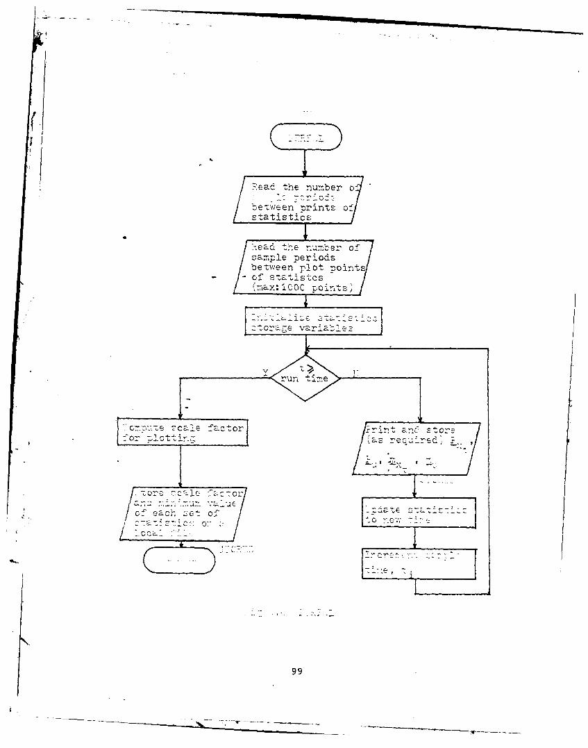
-~ead~ the num~ber o-,

betvween pot ints S I tatistcs

betN~leen plo pints

:o~~~- ,2c 1 j; e~~ea

-. I Z_,

Y .1

99 ir

jele-te deterriniAstic

cacuate e:;-envaiue states (as required)

subrouti-e

-aoculat steady-~a~

-ea r- n- i

- xc s: -

7~ ,

Uiser' srecifies whether or

100

feedback gain matrix, G*. Eigenvalues of the truth model F-c

matrix, the controller model F matrix, [F. - Kf Hf] (filter

poles), - Br G*] (LQ controller poles) and [F - Bf G*f - c C

Kf Hf] (LQG controller poles) are calculated if the user wants

to see them (MEIGN).

MEIGN (Fig A.6)

The subroutine MEIGN is called by CLQGRS to compute

and then print the eigenvalues of any given square matrix.

CKFTR (Fig A.7)

The subroutine CKFTR is called by CLQGRS to perform

the computations for determining the steady-state continuous-

time Kalman filter gain K as in Eq (2.13). This subroutine

deletes deterministic states from the filter equations as

described iD the Deterministic State Augmentation section

of this thesis. In addition, the user may select to use

the Doyle and Stein method to enhance robustness of the

bontroller. This is done through a call to qubroutine DAS1.

DASI (Fig A.8)

The subroutine DASI, when called by CKFTR, gives the

user the necessary design options to perform modifications to

the Kalman filter gain calculations that are described in the

Enhancing Robustness in Continuous-Time LQG Controllers section

of this thesis. The user selects the scalar design parameter,

q, and the matrix design parameter, V, and then must select

to calculate the modified Q(q) matrix. After observing the

101

r :.ead option; 1, 2, 3, 24

i-enter scalar designparameter, q

c~gnpara7-.eter,

--conte modiiedinput noise strengthmatrix (q,

-a t t',-I;.

-A. c CAS1

01,...... - a;-- : or

eta .- c. :c. :a n

1or -

, ce.e f~e~back cain

102

modified Q(q) matrix the user ban select either to exit the

routine or recalculate Q(q) with new parameters. Note, the

user may chose any option at any time in this routine and

therefore must insure that values are chosen for q and V

.ricr to calculating _(q) and that Q(q) is calculated prior

to leaving the routine.

a

CDTCON (Fig A.9)

The subreutine CDTCON is called by CLQGRS to perform

the necessary calculations to obtain the continuous-time op-

rimal steady-state feedback gain matrix, G* as described by-c

Eqs (2.10) and (2.14). This subroutine makes provision for

non-zero cross cost-weighting matrices by calling the sub-

routine PRIMIT. PRIMIT supplies an equivalent transformed sy-

stem of equations in which the cross cost-weighting terms are

zero. This transformation is necessary because the matrix

Riccati solver can handle only those systems of equations

*with zero cross cost-weighting matrices. A discussion of the

transformation is in Appendix C.

MYINTG (Fig A.10)

The subroutine MYINTG is called by RGS and DLQGRS.

It trovides an equivalent discrete-time representation of

any given set of F, B, G and Q matrices. That is, it computes

an returns thp state transition matrix 0 based on F. it

computes and returns Q. the discrete-time representation of

Q, which is an integral function of , G and Q. In addition,

103

C.-ED

-~--- L jj~ orc_ r arrcN

I (Eq (2.123))j

104

it computes and returns B, which is a function of B and the

integral of f. See Fig A.10 for the equations used in this

calculation.

DSCRTZ (Fig A.11)

The subroutine DSCRTZ takes an appropriately formatted

Qfrom CIQGRS) continuous-time LQG controller and discretizes

it using the first order approximations described in the

Doyle and Stein-Technicue in Discrete-Time Systems - 1 section

of this thesis. These approximations are then properly format-

ted for the performance analysis routine. In addition, this

subroutine computes and then formats for performance analysis,

an equivalent discrete-time truth model and, if appropriate,

the discrete-time approximation Rd= R t where At is the

sample time and Rd is the discrete-time approximation to R0,

the strength of the continuous-time measurement noise (Ref 10).

DLQGRS (Fig A.12)

The subroutine :LQSRS is called by RGS to perform all

necessary computations to specify a sampled-data controller

and then formats the controller for performance analysis as

discussed in the Sampled-Data LQG Controller section of this

thesis. DLQGRS calls XSU and then DDTCON to compute the

steady-state optimal feedback gain rratrix G*. It then com--c

putes a steady-state Kalman filter gain K, using the subrou-

tine DKFTR or the subroutine PKLIRC depending on whether the

user wishes to compute K from the matrix Riccati equation

(DKFTR) or to pick K directly (PKDIRC) (as in the section

105

i -- . . u m m m m a

gIn sma lerix e untm

DDTCON

Calcu;.Iate the Kalian Pick the Kalman fiLlterfilter gain gain directly

1av User seeformaneo f o ti l ala fil r gi

106

of this thesis titled Enhancing Robustness of Discrete-Time

Systems by Directly Choosing K.) Filter poles, LQ controller

poles and LQG rontroller poles are calculated (MEIGN) if the

user wants to see them.

XSU (Fig A.13)

W The subroutine XSU is called by DLQGRS to compute

the matrices X(ti), S(ti ) and U(ti ) as described in Eqs (2.95)

through (2.97).- Notd, XSU does not directly solve Eq (2.95)

through (2.97) but solves an approximation to their solution

forms as discussed in Appendix C, Programming Considerations.

DDTCON (Fig A.14)

The subroutine DDTCON is called by DLQGRS to compute

the steady state optimal feedback gain matrix, G*, for a-c

sampled data controller. Some data formatting complexities

involved in using Kleinman's matrix Riccati equation solver

to compute the G* are discussed in detail in 'ppendix C.-c

One involves computing values for the integral definitions

of X, S and U as described in the Sampled-Data Controller

section of this thesis (See subroutine XSU). Another involves

converting a system with a non-zero cross cost-weighting

matrix, S, to an equivalent one with a zero cross cost-

weighting term since the Kleinman matrix Riccati solver does

not have provisions for non-zero S (this conversion is done

by subroutine PRIMIT).

107

* --- --- ~ --- ----

C xs U

Read number of,

sub intervals-

I a=ze, DDTCON

f.r=O, X=O, U=O,,S=O Format system equations

f or Kleinman matrixRiccati equationSCompute -f., B.j for solver__

each subintervil - PRIM:I T

t ho, P j I Compute Kc steady state

I value from matrixCompute running sums Riccati equationof )_(ti), U(ti),

s (t.)_____I____ _Compute the optimalsteady state feedbackgain ma-tri.X,G-r

last NsubintervalN

Y Return

Print u(t,, (tji,

and S(t Fig i-.14 DDTCON

Fg A.17 ZU

108

IL

DK:FTR (Fig A.15)

The subroutine DKFTR, when called by DIQ-zS, corputes

the steady-state Kalman filter gain, K, for a sampled-data

LQG regulator as discussed in the Sampled-Data LQG Controller

section of this thesis. There is a provision to modify the

computed value of K by altering Q (the covariance on inpuz

nioise matrix) that appears in the matrix Riccati equation for

K. The modification is performed, when requested by the user,

by calling subrnutin§ DAS2.

DAS2 (Fig A.16)

The subroutine DAS2, when called by DKFTR, performs a

modification to -d (the covariance of the input noise) that

is a modification to the Doyle and Stein technique that is

applicable to sampled-data systems. See section The Ecle

and Stein Technique in Discrete-Time Systems - 2 -the body

of this thesis, for a description of this modificatior. DAS2

-is very similar to DASi and as in DASI, the user chooses op-

tions in order to enter a scalar design parameter, to enzer

a matrix design parameter, to calculate the modified _d and

to exit the routine.

PKIRC (Fig A.17)

The subroutine PKDIRC, when called by D1QlzS, z-rforms

t'.e necessary inrut options and computations to derive a Kal-

man filter gain K in the manner described in the 7nhancing

Robustness of Discrete-Time Systems h Directly Choosing K

109

Remove deterministicstates from controllermodel if necessary

SomaPerform Doyle andaStein robustness

penhancement technique,modified for sampled-data IQG controllers

Format equations flr r otn 1Kleinman matrix dicct euation solver

Compute Kalman fimeeragain for modifiedd

eforma. man filter 7 E i tis rou2ineaen matrix with e'sadded in locations

Fcorresponding to thedeterministic states 1- Enter scalar designparameter,q

.

• . :2- Enter matrix d esign(Re'urn z parameter,

-Compute modifiedQ(q)

'Fi Ir"-1 DI- Exit this routine

User decides whether-'or no. to perfor ( eur

Fig ..16 L-.-.S2

110

I I I I 4'

CED U G

1, 2A, 2B, 3, 4 QA=

1-Enter scalar design I Iparameter, q GCZA= cz

2A-Enter matrix design 0 0__parameter W fparameter __-_d- _RAign

2B-Compute matrix design1

3-Compute and print steady-state Kc=q-BIPdV= z

4-Exit this routine L B cz Et

, Return FA f t +BGc z Ht BtGcx]

lig A.17 P}DIRC L~Y

" L'_~ -~cz)-

ta

jGUA=[2czLT Gj

9 Fig A.18 FRIYAUG

111

section of this tlhesis. The user must specify the scalar

design parameter, q, and one of two methods for choosing the

matrix design parameter, W. W can either be chosen directly

or can be calculated as in Eq (2.129).

FRMAUG (Fig A.18)

The subroutine FRMAUG receives data in either the con-

tinuous-time or sampled-data LQG controller format and forms

the augmented matrices required by the performance analysis

algorithms described in both the Continuous-Time Performance

Analysis and the Sampled-Data Performance Analysis sections

of this thesis. That is, it forms Fa or aP ,.a or Bdaa G cr

Gda' Qa or Qda" and P xaV for continuous-time systems.

In addition, it also forms R a$ gcza Gua Ra and G are-cza ' --a -cza

simply Rt and Gcz in the upper left partitions of Ra and G-t CZ- -CZa

respectively. All other elements in R and G are zero.-a -czaIt is necessary to form R and Gc in order to use the Klein-

-a -cza

an matrix routines which require that all ma'trix arguments

be of the same declared dimension. Gua is formed out of ex-

pediency. It is the lower partition of the matrix.

It

;':hich appears in Eqs (2.47), (2.49, and (2.50). With C

t]-xzs de"' , z : G P . I.. elAminates the ur.--, defl -UU. -ua -aXa -ua

necessary multiplications associated with the upper partition

of the matrix above.

112

~~ !

Note that P v as defined in Eq (2.57) is calculateda t

only for continuous-time systems and then only when G in-cz

Eq (2.27A) is not equal to zero.

STCRED (Fig A.19)

The subroutine STORED is called by PERFAL to format

d ata from the performance analysis subroutine, PERFAL, for

storage on local files. This allows the user to store data

as a permanent file upon program termination and, later,

to recall the permanent files for printing or plotting as

required.

PRIMIT (Fig A.20)

PRIMIT is an auxiliary routine used by DDTCON and

CDTCON for optimal deterministic controller gain calculations.

It -transforms a given system of equations with non-zero cross

cost-weighting matrices to an equivalent system of equations

with zero cross cost-weighting matrices. The requirement for

and details of this modification are discussed in Appendix C.

CDTCON and DDTCON transform the resulting optimal feedback

gain matrix back to a form consistent with the original system

equations.

DLATIO (Fig A.21), MVECIO (Fig A.22)

These subroutines are auxiliary routines that are

callc " mst other subrcutines to perform input and output

of matrices and vectors respectively. Both routines perform

Zactions on the desired array/vector based on the value of113

A STEDPRMI

f 1=Z-.B U-1S T

Fis Y tore unlI. D

F-ig A.20 PRIMIT

OJlose tapDe files

Return

Fig '-.Iq STORED

MLATIO KYC 10

Read inp ut option f Read in'put o-ption1, 2, 31 4, 4 1, 2, 3, 4, 5

1-Read entire array 1-Read entire vector2-Read/print entire 2-Read/print entire

array vector3-Read selected array 3-Read selected vector

elements e lements4-.B:cad/print selected 4 -R ead/print selected

elements of array elements of vector5-Frint entire array j5-?rint entire vector -1

ReturnC R eturnD

Fig, A.21 r.MATIO Fig A.22 I.YECIO

114

mhree parameters, iO, KIN, KOUT. KIN' and :KOUT tell the rou-

tir.es which file to read from or write to, respectively. I0

can have any o4 5 values; 1, 2, 3, 4, 5. If IO= 1, the rou-

tines read all elements in list directed (and row by row for

arrays) form'at. '0= 2 7erforms the same read but also writes

out the entire array/vector. I0= 3 lets the routine read

selected elements in the array/vector. I0= 4 performs the

same read function as I0= 3, but it then prints the values

read. IO= 5 causes the routine to print out the entire ar-

ray/vector. Note that if I0 is any number than those listed

above, a call to these subroutines produces no action other

tharn a return to the calling program.

AUGMAT (Fig A.23)

The zubroutine USTMAT is auxiia-y routine used to

form augmerted matrices. Based on the flag F.0.M, AUG.T

either forms

,hen given the two matrices A and B and their dimensions.

115

edRead desired iorm- 1 esdead

0 eadror 2, read matric2es

i

aand

B

n07

t

tI-Form the augmented

matrix

r

i

cu2-Form, the augmentedmatrix

Return

Fig A.23 AUGMAT

116

A.pendix B

Software Source Code

This appendix contains the FORTRAN V software written

as a result of this thesis. The FORTRAN Y source code imple-

-ents the flowchar-zs -hai are specified and discussed In -

Pendix A.

Table B.1 contains a listing of the variables as used

4n the various sections of this thesis along with their FOR-

TRAN V counterparts ds used in the software.

117

TABLE B. 1

Correspondence Between Variables in Thesis andFORTRAN Source Code

Variables FORTRAN Variables FORTRANas in Thesis Counterparts as in Thesis CounterpartsIF FT exp(-F At) EAT

Bt BT Jo GQGTfTdr INTGA

G. GT j

4HT LIBd INTBA

-it QT Pxav PXVAt at

Lf -RT G cx GCX

G GCYG cy GCZB. G-c z G

B BCY

--c z BCZF0 FC

~R14 Ri"f t PHIT

I-xx PHIMwuuu FC

--c-Xu t DE TI1h'

GCSTR

RKFSS_,S S

FAU:-a= U U

_j PH!JGk=a B •BJ

" QA -I

-ua

PXA V Vax q S Q

MIXT

P XT

118

TABLE B.1 (con't)

Notes:

a. A "D" appended to the right side of the Fortran vari-

able indicates .that it is an equivalent discrete-time repre-

sentation of the variable. For example, BTD is the equi-

valent discrete-t%4e counterzart of

b. A "T" appended to the right side of the Fortran vari-

able or expression that designates a matrix/vector, indicates

that the matrix/vector is transposed. For example, HTT is

t'

c. An "I" appended to the end of a Fortran variable or

expression that designates a matrix/vector indicates -. at

the matrix/vector is inverted. For example, PEII is R_

--m

119

tbECK LOGRPPROGRAM LQGP(OJTpUT;S46TAPE6.OUTP U TrAPELBSS4 TAPEI3*64.ITAPE14s44 APE1664, NPU T4,TAPEIS6iP(0UT.TAP~fi-64 TAPE7)

C THIS PROGRAM PERFORM$ A PERFORMANCE ANALYSIS FOR THE LINEAR QUADRATICC GASSIAM CONTROLLERS DESCIIED IV DCX).'DT*FX+DU+CU AN1D A QUADRATICC COST FUNCTION IF DIFFERENT CONTROL. ALCOR17HN16 ARE SUPPLED THEC PROGRAM WJILL SfILL DO A PERFPRPIANCE ANALYSIS. THE METOI4OVOLOGY 1SC BASED ON THE PERF ANAL. SECTION IN CHAPTER 14 OF P. S. %AVIECXSC TO BE PUBLISHED UOLIJME 8 OF STOCHMODELS..EST AND CONiTROL.CC MANY OF THE SUIROLJTZNES USED FOR MATRIX MANIPULATION COME FROM THiE

C ROUTINES COMPILED RY D. KLIENMAN(TR-75-4. ONR CONTRACT IC h~eee±4-75-Cl067)CC IN THE FOLLOWING PROGRAM TRUTH MODEL MATRICES ARE TWO LETTERS WITHC THE LAST LETTER SE1ING -T- .CONTROLLER MODEL MATRICES ARE TUOC LETTERS ZNDING IN -M-.* -T- FOLLOWING APARTICULAR MATRIX NAMEC INDICATES THE MATRIX IS TRANSPOSED. -I- FOLLOWING A PARTICULARC MATRIX NAME INDICATES THE INVERSE OF THE MATRIXCCC COMM BLOCKS MAZNIDMAIN,IHOU ARE REQUIRED BY THE KLIEMAK ROUTINESC---INPUT FROM TAPEI* --- OUTPUT TO TAtPEll

CHARACTER ;SQZSREAL FT(S.S).IT(5.S).GT(S,S),HT(S.S),RM(S.S).

iPO(S.53.QT(S.S ).RT(S,S),CMtIO,1).CO2(1O.):GCSTR(S,SI )W SS ),RM2F(5S;.M5)Uu1 (ry~SSTT (SS.mt~

GcI ,CKS)5bGCZ(sS l.OA(1,.I,).PXA(1* 16) PXvA(I.110).I MUOIJT(s ).MX'TO+(S),PXTUtS) PUOUTS.DlIkI GUJA(IO.1S),MXAMIMS),XAkMAX(t).MUM4(I mmmU ilt.1 PXTIN(g) PXTh4AX().PU"MNS),PUMAX(S).CA(l.IB).I Rokis to) iC(iI).ICZ(SS1.6CV(5 $),FCfS,S),

INTEGER IFLGCZ. IRYREAL I'W~c)COMMON 'OR"tIM' RNTIME.DELTIMCOMMO'N /MAIN2IoCOMBCOMMON /MAINI/NDIM.NDJMi,COMICOMMON / INOU.' KIN,bzOUT.CPUNCHCOMMON .MArN4/NrZMD1M3COMMON /MAUNE' MSGCOMMON 'MAIN60 ICITDZCBM.ICFA.ICGAICCMICCTZCOAIRFA,IRFM,4RFT,

I IRHTIROA,1O,LG.IRM,IMDTSC

DATA UNA.UMt,UMC,UMD,U? E,UMF P668ZO.8-DATA OA,COPMI,COM2,FA,DR,GA,PXAPXVA n960.0/DATA UU3.U1J4 /Z920.61DATA UMI.UM,uR3,UM44.U#MS.U(M.FT,BT.CT,HT /RSSZ.8/DATA 64UU.UXX,FMBM,6MPO.OT.IJXU /220~.0/DATA RTGCSTR,RICFSS,CCX,GCZ h/L25.6/DATA UVI.UUJZ,XO,MXA,MU /3020.01DATA RM.GM.HM /7S%6.*iDATA XFLOCZ /V'

CC

K0UTs6KPUt4CH-7KOIM-S

HDIM2.IONDII'3- Im

CCCt 2*9212922MAth PROGRA FOLLOWJS 22222220--- IRXX. ICXX INDICATE *OUS.COLUMNS OF "ATRIX XXCC*2x*2TH1S PROGRAM CAN HANDLE UP TO 1"S DIFFERENT COMNINATIOS OF

DC 391UNTIME,DELTIM.AND UNSPECIFIED PARAMETERS&IRITCKOU.II)

'

120

la rRAT(A1, ,,j Sp UBR'LG MRroF R AT ( O TLT, , r , M M w~ o ,*

CAL INpUTA F1,T, ,

IF dlO.EQOe) THEhGO TO Z33END If sox GCZ,SCY,3czFC YD*

CALL RG~ C T jjme u p u l , I

UjRITE(Kou,)Do You VZSH TO CALCULATE TtC. EIGENVALUES OF TH CL.OS

IED-L.OOP STATE TRA4SITIO" TWARIfl USED INI THE

PERFoR1MANCE ANALYSIS

I(APPL.ICABLE TO SOT% T"E COTNOSTM AMD SAIPLED-WAA CASEI

READtK1h,1ZMSIF (ISO.EQ.*') 114EN

WATIE(OUT.2)THE. CILOSED-LOOP STATE TRANSIION MATRIX EIGENVALUES

NSAVNrDIA

CALL MEGcM W3W4IRFA.UI%EHD I'qNSAVN'D1~1 .NSAV~ IEND IFURITEOUT.t)T;EY oURITE OUT , VP ) PERFORM' THE COVARIANiCE ANALVSIS..

TYPE

I h TO SKIP IT>'RADK(. x)"sCIF (N TE00 TO a932END IF

CALL F RFAL( ?RFCZYK(,C U )A, PXA. IFLCSD.

I WU, V

2932 CONTI"U

B933 wRT(O1,VRGA TRMIN'ATED, 940 ORE-ImPUT

DATA'

SUEK R0UT1INE STORED( 1UH,RN IMEDEL IM IFSTCL. 15 1ZSZD

5TEC TonE 5 bEL.STII'. R14.STORIS ,NDIRS)

CTI41S Su OU ISTORSISZl PL T o To LOCAL FILES. TAP12 TAPEI3.

* CTHSSjoTX STRE PLTP DOR WER -m4T STORAGE. isxxsZ IS THE SIZE IF THE

CDATA RRAYS,STOR X. D IM IS T 1E CA 'LI . PROGRIn+ Dll E HE O

tTHE ARRAYS. NOTE THAT RUNTIPS IETR2 11UE E TOT

CH RU. TE LAST VNR'INEC

C NIER Of DATA POINTS I" H h AO H IENH

C DATA FILE Is THE SCALE FACTOR DFOR THE DATA N THE F t

C EXT TO LAST ENTRY Is THE Il1U"VUEOTHDAANTEFL

D i E tSlc O S T OR T ( D I R &g ) ST OR 3 L N4D I 1%6 1 ST OR 4 C ) R S N 1 45

If tIFSCL.E.0 THE"

C PUT A RUN HEADER ON T E I TAPE3O

OpENCUMIT .x.ERReIS.*IP;E1':RECLSSb)vlar(UMTIS4ERR~:#FILE*1TAPEIS,RECLS0)

URITSMt1,l1 jICRNRN"TIME,DELTI,,I~az

WRITE(16.itilet rm"ATC'

END VFif (IVSTCL.LTAI1 THEM

c CLOSE PILES AND PUT1 END or FILE "ORKER OM TMiCH.

CLOSE(StEARft' I

CLOSE0I4,ERR-16CLOSE(MuERR IS)RETURNEMD IFuRTTE(Ia 169)(T0RI'V(

j.I1S

121

RETURNto WRITE (OUT.X)'AN ERROR HAS OCCURRED IN TrHE STORED ROUTINE'102 FORMAT(3(4(' 'ES6f,)

END

SUBROUTINE INPUT tFT,IT.GTHT,FMIN,G.HrK.POQOTD~RT.RM,XoI * IUU. UXXILJ)

CHARACTER IMSQX6O,KSG*SeREAL FT(MDIM.NDIM),3T(NDIM.NDrN3.GTCND.NDN),TNDM,1Dr1),HI(ND

I CR(NDIM,ND1N).UXU(hDIN,HD1M).I PO~tNDIP,NDIM),OT(NDIM,HDIn,RT(D1N,DIM),COM1(),CPK2(1)

COMMON 1MA1N8Z/COM2

COMMON / !NOU' KI1HOUTKPUNCHCOMMON /MfAUf~NS SCOMMON fMAIM6/ ICIT. 1CBM. CFAICGAICGM.ICGT.ICOA,IRFA. IRFM,IRVTf,I IRHT,IRQA,I0,LGG.IRHIi,H~MDTS

C ICFTIRFr.ICFM.IRFM.IRT.IRT.IRDMIRI.IRCT.INrr.IRGN.IRFNC rRX-IRIROJC.ICG,IPR-ICRIT.IRIJXX-ICX)(.IRFM,C -IRWIUUU- ".ICMCIIRFT ItlIf.RC.CTIGZI~TC 10 IS A INPUT ROUTINE PARAMETlER--iIREAiDDf-READLPRINT.c 3%. PRINT ONLY. 4-PIJICH

IqSA'J*NDI~q

C IRX.IRF. IRGXCO CGM. IRROrCM.IRNT, IRWXX.ZCWXX.1RFMqC IRUU.!ICUUU-ZCkM ICHT.IRFT ICHIR'l.IRCZ.ICBT,IC CZ.?R,C 10 IS A INPUT ROUTINE PARAM'ETA--I-READ, -REA LPRINT,C 3- PRINT ONLY. 4aPU4CHC

NSAV.NDIIQMDIMI -hDIMIF (LQG.EQ.I) THENhRIECKOuT~t )MSOIURITE(KOU ,:)'THE 1/0 OPTIONS ARE I,1,2 3.4 S.6 .......URITE(KOUT.: ) * -READ ENTIRE ARRAYzUEC+OR.2-AEAD AND PRINT'URITELKOUT.:)'EMTIRE ARRAYVECTOR, 3-READ,AND 4-READ AND PRINT'u1RIT JKOUT,%)'SELECTED ARRAY/VECTOR ELEMENTS, 5 PRINT ENTIRE'JRITE CKOUT,Z)'ARRAYVECTOR. 6 OR GREATER NO MORE INPUT TO'WRITECKOUT,:)'DE MADE.'URITE(KOUTD: )?SGIURITE(KOUT,Z:PSELECT WIHCH MATRIX YOU WISH4 TO ENTER.'URITE(KOUT,*)'lY ENTERING THE ADPROPRIATE NUMBER. 1-VT.Z-BT'URITrE(KOUT.Z)'3-GT.4-$T.S-FM.6-BM,7-CM.8-MR.9-PO.1S-0T,11-RT,)-WRITECKOuT.:,'12-OM,13-R.14-XO.1S-W-u;UXXI?-uXU,1u-EGuATE ALL

URITECKOUT,t)'COMTROLLER MODEL PqATICES TO THEIRWRITE(KOUTZ)'TRUTH MODEL COUNTERPARTS.2 1--NO AORE DATA'URITE(KOUT.:)'ENTRIES TO BE MADE. as--STORE ALL MATRICES ON TAPE?'URITE(KOUIT.S:21- READ ALL MIATRICES FROM TAPES,URITE(KOUT.1 )M'SGIWRITE*KOUT.1 )MSGIURITECKOUTZ)'hIRITE(KOUfT.2)-FOR SAMPLED DATA MEASUREMENTSENTER EITHER A COt4TINU

IQUS RM TO USE TO APPROXIMATE THE DISCRETE TIME RMD(RMD.RMSAMPLEITIME. OR ENTER THE DISCRETE TIME RMDIIIRITE(KOUT.* )MS61URITECKOUT,: )"SGIVID IFDO 95a 119uya',193UNITE CKOUT33333),

23333 FORM'AT(A0,,')URITEIKOUT,I'E"iTFR CODE FOR WHICH ARPAY4IVECTOP TO SE INQUT'#READ(KIHDB )IUC4MA

CCgzZTRUJTN MODEL INPUT

I RITEKOUT,X3'ENTER-In OPTION. FT MATRIX SIZE>READ CKIh.Z,ENDw27 JIO.ZftF?MSO.'TRUTH MODEL F MATRIX ENTRIES'CALL PW9ATIO (FT IRVT 'IRFT.IO.CIN,KOU?.NDIM,NDIMI)IF (104.6.S TWtlRETURNEND IFGo TO 933

122

2 RITE(KOUT.2)'ENTER-1/O OPTIONS. COL.UMN SIZE, OF IT')'READ(K1#1,x.END.2?3Z0,IClT-IiSG.'TRUT14 MODEL I MATRIX ENTRIES'CALL flIATIO C3T.IRFT.KCT,1O.I.RzOT,NDIINDrII )

IF (IO.EG.S) THENRETURNGo TO 92

3 URlTE(KOT,2)'EITlEU-I,0 OPTION. COLUMNt SIZE OF GT>'READ(KlN.2,EMD.27)IO. 1CG?MSG-'TRUTH MlODEL 4 MlATRIX ENTRIES'CALL MMATIO (CT,xRrr,ICGT.1o,Kl,KOJT.NDIN,NDIII)IF (O.EQ.6) THENRETURNEND IFGO TO 98a

4 URITE(KOUT.1)'ENTER- 1.*0 OPTION, ROW SIZE OF W01'READ(KIH,2.EMDo2? 310 IRHT9MSG~'H MIATRIX ENTRIES'CALL PATIO (HT.ZRHTIRFT,1O.I.KOUT.DI.4DZft1IF (IO.EG.S) IWEIIRETURNEND IFso TO 9"2

C3MZ1NPUI CONTROLLER MODELs URlTOU.T,)'EM!ER-1IO OPTION, FMi MATRIX SIZE>'

REAb(CIM.%.EMP7IO 1. 1RFMMSO'.'CONTRCLI.ER M ODEL F FATRIX ENTRIES'WRITE(KOUToW)ENTER THE NUMIER OP DETERMINISTIC STATES IN THIS MOD

11L0'READ(KIM l.END-273NUMD'CALL MMAf 10 (FM.IRFMIRFM.ZOSIILCUT.NOIN.NDZNI)IF (I0.Ea.@) THEMRETURNEND IFso TO sat

6 UAITE(KOUT 9)'ENTER-I/O OPTION, COLUM~N SIZE OF BM)'REAM(MUZ~ND-M7 IO.IC31MMSG.'COMTORLLER MODEL I MATRIX ENTRIES'CALL MATIO (3I .IRFIC 1M. IO.KN,KOU.N0,.fDIHZI)IF (IO.EQ.O) THENRETURN4END IFGO To 932

7 VRITEIKOU .t)'ENTER-1/0 OPTION, COLUMN SIZE OF QM)'READ(KIM,x,END.o27)IO, ICCMRSG*'CONTROLLER MODEL G 14ATRIX ENTRIES'CALL MPIATIO (G", IRFM. ICGPI. IINKOUT,NDII!.NOZMt)IF (IO.EQ-S) THENRETURNEND IFGo TO 982

a hRITE(KOUT,2)lENTER 1/O OPTION.ROW SIZE OF MW)READ (KIM, t,EKD.7) 10, IRNMSG-'THE CONTROLLER MODEL MEASUREMENT MATRIX, IW, IS'CALL MMATIO(HM.lRHP , RF-K1, I,KOUT.MDIM,NDIRI)IF ( IO.EQ.6* THENRETURNEMVIFGo To got

3 UAITEUOUT.1)'T MUST NE ENTERED TWEU OPTION I PRIOR TO USING THISI OPTIOM.0O YOU VISH TO ABORT THIS OPTION, V OR N)'RE^V(KIh 97.EKDe27)ftGIIF (MS41.Q.V) THENGo TO 932END IFURITE(KOUTDP*ENTER 110O OPTION,IRFT IS ASSUMED SIZE 0F P0>'READ(II,%,EKD'E7 310MSG411'HC INITIAL COVARIANCE MATRIX PC, Z61CALL "MATIO (PO IRT,RFT,ZO,KIN,6 ,DIM.MliM)IF (IO.0O.4) THS~RETURNEND IFGO TO 932

WShRITE(MOUT.~)'ENTER 1/O OPTION, ICQT IS ASSURED SIZE OF 07)'RCAD(KIN.S,EMD-27 10MSC.'TNE INPUT NOISE STENOTH MATRIX 0T IS-CALL RMATIO (OT,ICGTICGT,.IMKOUT,NDIIDNDIN1)IF (IO.0Q.61 THENRETURNEND IFGO TO 332

123

it 6URITECKOUT.2)'ENTER 1/0 OPTION.IRHT IS ASSUMED SIZE OF RT>'READ(KIH.t.END-R7 )lOr-SG-'THE MEASUREMENT NOISE STRENGTH MATRIX RT IS'CALL MMATIO (RT,IRT.IRHT,IOKlN.*OUT.NDIr,.NDIMI)IF (IO.EO.S1 THENRETURNEND IF,GO TO 932

12 URITE(KOUT,Z)'EHTER I/O opIoNCam IS ASSUMED SIZE OF OR),READ(KINjz,END-27)I0MSG- 'CONTROLLER MODEL INPUT NOISE STRENGTH MATRIX, OM'CALL AMTIOO9.,ICGN,ICGM.IO,I,OLT,NDI9.NDimi1)IF (I0.EQ.G) THENRETURNEND IFGo TO 932

13 URITE(KOtJT.2)'ENTER 1/O OPTION, IR4M IS ASSUMED SIZE OF R19>-READ(KZIN. z.END.27 )1OMSG. 'CONTROLLER MODEL MEASUREMENT NOISE STRENG.rT MATRIX, RM'CALL MMATIO(RN. IRi'P, IRNM.O1.c.OUr.NDIN,,WIML)IF (IO.EO.S) THENRETURNEND IF00 TO 92

14 URITE(KOUT X)'FT MUST BE ENTERED THOU OPTION I PRIOR To USING TI-ISI OPTION. bo YOU WISH TO ABORT THIS OPTION, Y OR N)'READ(KIN.97,END.87 )MSGIF (MSG.EO.IY') THENGO TO 982END IFWRrTE(KOUT,%)'EKTER 1/O OPTIOM,IRFT IS ASSUMED SIZEOF XO>'

READ(KIN,*,END.27 )IOF.SG-'THE INITIAL STATE VECTOR, XO, IS,CALL MVECIO (XO. IRFT. IO,KIN,KOUT.NDIM)IF (IO.EQ.@) THENRETURNEND IFGO TO 92

Is URITECKOUT,S)ulq MUST BE ENTERED THRU OPTION 6 OR 17 PRIOR TO USIN1G THIS OPTION. DO YOU WISH TO ABORT THIS OPTION. Y OR N),READ(KIN.g7,END.27)MSGIF..JMSG.EO.'Y') THENGO.TO 982EIRD IFWRITE(KOUT,Z)'ENTER 1/0 OPTIONICBM IS ASSUMED SIZE OF UU)'READ(KIN.*,END%27)IO

MSG-'THE CONTROL FUNCTIO" COST WEIGHTING MATRIX. WU'UCALL MMATIO(UUU,ICBM.ICBM,IO.KIN.KOUT.NDIMNDIMI)IF (IO.EQ.0 ) THENRETURNEND IFGO T0982

is URITE(KOUT,Z)'FM MUST RE ENTERED THRU OPTION 5 OR 17 PRIOR TO UtSINIG THI1S OPTION. DO YOU WISH TO ABORT THIS OPTION, Y OR N),READ(K1lN.97.EID-27)MSGIF (MSG.Ea.'Y') THENGo TO 98END IFURITE(KOUT.z)'ETrER IeO OPTION,tRrM IS ASSUMED SIZE OF hIX)'lREAD(KZN.2,END.27 )IOMSG'THE STATE COSTEIGTINOMATRI xxo

RETURNEND IF00 To 333

13 URITECKOU? t)'ALL CONTROLLER MODEL MATRICES HAVE BEEN SET EQUAL TO1 THEIR TRU+H MODEL COUNTERP ART S'WRITECKOUT,*)'FT,BT GT HT OT.RT MUST BE ENTERED PRIOR TO USING TMIl

IS OPTION. THE NUMBER bF bETERMINISTIC STATES MUST BE ENTERED INI THIS OPTION(FOR CONTROLLER MODEL).'URITE(KOUT,2~' DO YOU WISH TO ABORT THIS OPTION,Y OR N)'READ( KIN,97,END*27 )MSGIF (MSG.EQ.'Y') THENGO TO 933END IFWRITE(KOUT.X)'ENTER THE NURBER OF DETERMINISTIC STATES IN THE CONT

124

IROLLER MODEL)'READCKIN,Z.EHD.27 )W4~DTSIRFII.IRFT

97 FORMAT(At)ICRM-~ICBT

CALL EGU1ATE(FM,FT,IRFT, IRFT)CALL EGUATE(BM.RTIRFT,ICVT)CALL EQUATE(GIM.GT,IRFTICGT)CALL EQUATE(14q,HT,IRHT.IRFT)CALL EOUATEON.OGT.ICGT.ICGT)CALL EOUATE(IZMRT, IRt(T. XRi7)

17 LDRITE(KOUT.2)'NOTE THAT FM AND IM9 MUST BE ENTERED THROUGH4 APRPRIlATE OPTIONS PRIOR TO EXECUTING THIS OPTION. DO YOU WISH4 TO ABORT TIMIS OPTION, Y OR H)'REiD(Klh.97.ENDaE7)MSGIF (MSG.EQ.'Y')TIENGO to 988END IFWRITE KOU?,*:'ENTER 1,10 OPTION, IRFM X ICBM ASSSUMiED SIZE UXU)'READ(KIN.t.END.27)1OMSG-'T4CF CRO9S (STATE-CONTROL) COST PSEIGHTING MATRIX. UXU'CALL MMATIO(UXU.IRVM.ICBM.1O.KIN.KOUT.iWIM.NDIMI)IF CIO.EC.S)THEMRETURNEND IFGO TO 988

ft URITECKOJT 1)' THIS OPTION STORE$ ALL MATRICES ON TO TAPE?, DO YOU1 WISH TO AiORT THIS OPTIO,Y OR N)'READ(KIN.97 )MSG

IF (MSG.EQ.'V'1TKMNGo To 928END IF

URIrE(7,ZRF7. lCD?,ICCT,IRH4TIRFM,ICDPi,ICGM,IRHM,NUMDTS

l(I(7C,*),J.TI,R),Jw1,IRFT), ((3C1.),J.1,I3),I.1,IPTq) -,R1URITEC7,*:CG1,J,J),l,ICGM I.IRFM)(4MC1.J),J-l,IRFM),I.1,IR1-J.1.ICBM),I*1,ICIN),C(UXX(I,J),J.1,IRFM),I.1,IRFM)4URITE(7,Z)( (OTC 1,J),J.1, ICGT). I-1,ICGT), CRT,J)J-,IRT2,141,IR

URITEC7,1)CCUXU(i,J),j.1.icIm),i.1,rRFm)GO TO 982

21 WRITE(KOUT.1)' THIS OPTION READS ALL MATRICES FROM TAPES, DO YOUI WISH TO ABORT THIS OPTION, V OR N)'REA.DCKIN,97)MSGIF (MSG.EO.'Y') THEN

GO TO 982END IFWRITE(KOUT.1)'DO YOU WISH TO REUIND TAtbES BEFORE THE READY OR M>'READ C11N,9? )19IF (MSG.EO.'Y') THEN

REWIND($)END IFREAD (S. t.END. 1003) IRFT. ICIT. I CT. IRKTIRFM. ICBM. ICGM, IRM. ". DTSREADC8,Z,END-1*3)(FTI.J) J1.IRFT).IIRFT),C(BT(1.J).J.L,1CI

RTEAD(B.?.END*19633) (OTI.J)I. I T) (.ICT,((RT.J2.JRFT.IIRT),s.IRT(F(OM(I),JI,IGM),I.Ic )c(M(J).J1.I,1p,.q?9.IR

I I.I,!RII4Pi).RFM

READ(S 2)1(UXUtIJ).J'I.ICIM),I.I,IRFM)G0 TO 682

10e33 WRITE (KOUT, t'END OF, PILE ENCOUNTERED DURING READ OF TAPER'982 CONTINUE19 CONTINUE

NDIMI*NSAVRETURN

27 10.8

( 'END

125

tD-c mm U

SUBROUTINE MEICNCA.AREV.AIEUC:URSZA,Wnl1CHARACTER P.S G%6DIIKESSIOtA(DI.D).AREVtNDIMN.AIEV(NDIN ),LIL(NDIM,NDIM)DIMENSION COM(l),COM2(I.)

COMMNON / INOUI KIM,KOUT.PU1CHCOMMON4 /RAINZ/ COME

C THE CALL1N^ ROUTINE MiUST SUPPLY A WORKING IiATRX NDIM X HDIM --61M1CUZVFIND THE EIGENVALUES OF A A-9~ TELLS THE ROUTINE TO CALCULATEC EIGENU-ALUES ONLYC "DIM MUST BE THE DINEr'SION OF A IN THE CALLINa PPOGPA-!C CURSZA IS THE CURRENT SIZE OF A

CALL IDrTCCURSZAI,l)C Umi' .1 CUIPSZA X CURSZA

* CALL EIGEN(CUPSZAAEL.AE.WEUi.4T)

NSAJ-DIImDZNI.NDINMSGO'REAL PARTS OF THE EICENVALUIESCALL MVECrO (ARE CRZ.1.I.O~TtDMMSG. ZYIAC PAR'T'S OF THE EICENUALUES

C CALL RVECIO (AEUSAII.O1~~m

tDECK CDCOtISU BRO UIJT NE CDTCO M1(FM N i x ,u u m .i t c m w l , ma*U3WM.m uI IJDIMf4*U ,UXUPR) p pV

1,GC STR(MDIMDNDIM,)

DIMENSION comm i),coPm2(lICOMMON PImAIN2,'COeCOMMON /MlAINI 'NDIpM. DZN:, COmICOMMNON / ThOU/ rZIN,KOu?*KPUNcHCOKMNON 'NAUNSI MSG

C

CIZIDE-ERMI1NZSTIC CONITROLLER GAIN CALCULATIO --- MODUJLE * 1CC. THIS MODULE COMPUTES THE STEADY STATE DETERM9INISTIC CONTROLLERC GAIN MATRIX. GCSTARw (WUI) 3,T) cKCSSPM). UUI IS THE INVJERSE OF Tc CONTROL COST IEG44TING MIATRIX, KCSSPM IS THE STEADY STATEC SOLUTION TO D(C/l(M)K)(C(M+U;(C(M(UI(f.)C (KC), WXX IS THE COST WEIGHTING PATRZX ON THE STATESCC KLIPHt ROUTINES ARE EXTENSIVELY~ USED IN THIS MODULEC TRASFORI SYSTEM SO TH4AT UXU h9T%6 CAN STILL. BE HANDLED ByiC KLEINMPAN ROUTINES, SEE KWAKERNAAK AMD SIOAN'S BOOK. PAGE 322

CALL PRIMIT(UMI,.UUU.ICIM,CCSTR.UXU.IRFM.3UN.FPRII,X.UXXPRM.

C HIOW HAVE FPRIA, U)OCPRM CAN USE RICCATI SOLVER FOR KCSSPM

CALL TRANS2( IRVPI.IC3M.BM.W1M)C UPI83T ICBMI X IRV"

CALL EQUATE(W NI.UU. lCRNICSPI)C CMrmV DESTROYS THE CALLING ARRAY

CALLCNV(CMB.PlU3I.'TC UPK3'%AJUI ICBMI X ICBM -- 4 IS A" ERROR INDICATOR

IF (NR.NE.ICIM) THEMPRI~t,,Am ERROR OCCURRED IN INVJERTING WUL. PRI.,MR,IIC5PI',ICVMEND IFCALL EQUATE(UMI VN3 ICRI.ICRMI

C WUNI.UU SAVE FOR CATEA COMIPUTATIONSCALL liATICUN3 hIN!,IC3PI ICIPI,IRFNMUPI4)

C UMd.(WUUJI)(DWT) HCIM X IRFPIC t4OW CALL RICCATI EQUATION SOLVER

CALL PIATI(II9,UI4 IRFMI.let" IRFPIumv3C uPI3.RPI(WuU)(RIT) IfiR K IRffi

CALL RC IRFP!,FPRIR.UNl3,bIXXPRM,UNE.UI6)C UPIE'KCSSP! IRFM X IRFMC U'.-3'(UI(P)(CPP)-IDONT USE THIS RESULT

RSQ-eKCSSPH FOR THE DETERNIIISTIC CO"TMOLLER IS'toes

126

NSAU-NDIR1NDIMI-NDIMCALL MATIO(UMaZRFM.IRF, IOKIN,KOUT,DINDINII

C HOW CALCULATE OPTIMAL GAIN MATRIX GCSTAR, NOTE I NEED THEC NEGATIVE OF GCSTAR FOR THE !ONTROL LAW GENERATION FROM AN LOGC CONTROLLER. AND THIS UILL 1E THE tCX REQUIRED IN THE PERFORMANCE

,€ ANALYSIS ROUTINENOIM1*H~SAv

C NOW KAU KCSSPM , CALCULATE GCSTR-UUUI(SMTCKCSSPM)VXUT)C RECALL UMUI IN WMI

CALL MAT4A(BM.WUNIC|M4 RFN. IRFM.UM4)CALL TRANS2(IRFM, ICDR,UXUUR3)CALL MADDI(ICBIZ.RFM, 't4.UM3.UMa,CI)CALL MPTI( I,.UWM2,ICBMIC3M,IRFM,GCSTR)HSAV*1NDIMIKDIMIi-sDIM

C CSTR iCNR X IRFt: C C RSG-'WE OPTIMAL STEADY STATE FEEDVACK GAIN MATRIX, GCSTR'

CALL MRTIO(CSTR.IC1NIRFM.10.KIN.KOUT.NDIAM.DIIf1)HOIMI -HSAU

CEND

IDECK CKFTR -SURROUTINE CKFTR(FM.GM R HM NUNDTSRKFSS Q UN.UM2,

. S~UM3,1UM4,US,UM'Gt,IRFFD, IRM.&GF,H.3.1f,fl

C CALLING PROGRAM MUST SUPPLY EIGHT WORK SPACE ARRAYSCCTHIS ROUTINE CALCULATES THE KALMAN FILTER GAINS UHENC GIVEN THE FM,Hr, QM AND R MATRICES AND THE NUMPER OFC DETERMINISTIC STATES. THE CONTROLLER MODEL MUST NEC SPECIFIED SUCH THAT ALL THE DETERMINISTIC STATES APPEARC FIRST AND TOGETHER, TH4AT ISCD/DT(Xi,X2,....XK,XL,XR ....XN)T I fol]| ,

C WH4ERE XL THROUGH XK ARE THE DETERI! ISTIC L LS NDTHC REMAINING STATES ARE STOCHASTIC. F1 IS K X K. AND F2 IS N-K xC "-K, AND B1,B2,AMD G2 ARE PARTITIONED ACCORDINGLY.C THIS ROUTINE FIRST STRIPS OFF THE DETERMINSTIC STATES THEN COMPUTESCAND RETURNS KALMAN FILTER GAINSFOR THE REMAINING STATES.C THE KALMAN FILTER GAINS FOR THE DETERMINSTIC STAES ARE SET TO ZEROC AND THE KALMAN FILTER GAIN THAT IS RETURNED IS 0CC UHERE THE DIMENSION OF THE ZERO VECTOR IS K AND THE RKFSS IS THEC STEADY STATE KALMAN FILTER GAIN MATRIX FOR THE N-K STOCHASTIC STATES.C THIS AUGMENTED MATRIX IS RETUTNED IN RKTSSC ALSO NOTE THAT IN ORDER TTO GENERATE THE KALMAN FILTER, ONLYC MEASUREMENTS OF STACHASTIC STATES ARE EEDED SO THE H MATRIX ISC REDUCED ACCORDDINGLY.

CHARACTER MSGS .RSG1t1DIMENSION F2(NDIPNDIM)oH2(IDIMDIfi),F iCDIMNbIM).SM(NDIMNDIM,I R(I I' NIM).HM(NDIMNDIM),VMltNDIM.DIM),O(DIM,NDIn).I UM NDM.NDIM).M3(NDIM,DIM),UM4(MDZMNDIM),U SCRDIM,NDIR)I ,uMS(NDIM.HDIM)REAL RKFSSCDIRNDIM),vR(NDrmNDIm)DIMENSION COMI(t) COM2(1)

': OtOMqo 'MAItNI-fD!M.NDIMICORI

COMMON I INOU/ KNoKOUT,KPUNCHCOMMON Ar"AUNSo "$G

CC:g*KALMNA FILTER STEADY STATE OAh----MODULE I tCC RIFSSaCPMSS)(HMT)(RI), UHERE PM IS THE STEADY STATE SOLUTION TO THC RICCATI EAJATION D(PM)/DT.FCPM)PM(FMT).GH(Q)(GMT)-C PM(HMT)(RI)(HM)(PM)CCC ttzgtZUDELETE DETERMINISTIC STATES, AND ---TRANSPOSE THE FEC MATRIX FOR TKE RICATTI SOLVER SINCE IT TRANSPOSES THE CALLING ARRAY)

WRITE(KOUT,I)'IF YOU PLAN TO USE THE DOYLE AND STEIN TECHNIQUE PCIR THIS RUN YOU MAY WISH TO MO.DIFY THE VALUE OF NUMDTS, THE MUnJERI OF DETERMINISTIC STATES. DO YOU WANT TO CHANGE J1.DTS? Y OR NtI).READ(KIH,11)MSGt

NUMSAV-NURDTSIF (MSGl.EO.'Y') THENURITE(KOUT, I EH TER THE 4EU VALUE OF NUMDTS FOR THIS RUN>'READ(KIN,)NU)DTSEND IF

127

:ADS.NufMDTS41Do 2112 I-IDS.IRFM

_I II I-HNUMDTSV DO 2112 J.IDSIRFM

JJ.J-NUfIDTS

1RFB IRFMi-MU!WTSDO £113 I.1,IRHiDO 2113 J.IDS.IRFMJJ-J-NU!MDTS

C NOW FORM R2,GE

DO 2114 J.1,ICGS

DO 2115 I*IDS,IRFM

DO 2115 Je1,ICI'P115 UN4C!I.j'~sDmC1 3)C UIM4 &92 IRF2 X CB

IRHH. IRHI!CALL MAT3(IRF2.ICGi.U~1,O,UM2)

C U,2vGMC~(0lG) lAP-I X 1R72 -- USED AS O'1IN KLIEHMAN RICCATI ROUTINEURITE(bzOUT.*)'DO YOU WJISH TO M ODIFY 0 BY THE DOYLE AND STEIN TECNIIIOUE, Y OR W)READ CKIN.I1)1iSG1

11FOR.9AT(AI)IF (MSlC.EQ.'Y') THENCALL DASl(L!M2,UM4,UM1,IClM,WM3,IRFM)

END IFMT& ICALL EGUATE(WMPI,RIRH2,IRH2,

C GMINU DESTROYS THE CALLING ARRAYCALL GF.IN(IRH2,IRH4,hM1.W 3,MRHT)IF CMR.NE.IRI42) THENL1PITE(KOUT.)'NR.',NR.'IRH2-',IR42URITE(KOUTS)'R-INVERSE IS FOULED LP'END IF

* C UN3' RI IRH2 X IRI42CALL TRANS2(IRH2,IRF2,H2.UM4)

C UP.4- MET IRFE X IRH2CALL MAT1CUr4,W1M3,IRF2,I1i2,IRH,pqS)

C LIMS- H2TCRI) IRF2 XC IRH2CALL MTCW'S.H2,IRF2,IRH2,IRF2,U13)

C 6 M3- H2T(RI)CH2) IRFE X IRF2CALL fRIC(IRF2,F2,UfM3,UM2.uM6.U'94)

C !IOW CALL RICCATI EQUATION SOLUERTO GET PASSC U%*-PSS IRF2 X IRF2

CALL MATIC61ME.URPF,IRF2,IH2,I)C UM1.RKFSS IRF2 X IRH2

10-SC FORM' RKFSS WIT4 ZEROS ADDED FOR DETER. STATES.

PRIMTZ. '".DTS-. t4tDTSIF (NUMDTS.NE.G)THENDO0 2119 J*1.1RI'DO0 2118 I.1.NUIIDTS

2111 RKFSSdI.J)&SDO 3119 I*1OS.!RFMII.! -NUtWTS

2119 RKFSS(I.J)aMbIl(II.J)ELSECALL E0UATEIRCF5SS.W1.IRFMIt$4t'END IFMSG.'STEADY STATE KALMAN FILTER GAIN MATRIX.RKFSS'CALL MMATIO(RKFSS.IRF9,IRHM.IO,KIN.KOUT.NDIM,NDIM,NUHLb'S .NLJSAV

END9DECK FRMAUO

SUBROUTIN4E FR?AUG(O.R,FT,BT.GCZ.HT.GCX.BCZ,FCCC-V,ICYGT.KCPO,I FA.BAGA,GA.GUA,WM1I,UM2,UMAW'i3 U'CWID,WFE.L?rFI MXAPXA.RA,PXUADGCZA, IRY.IFL6,CZ,IFLGSD)

C THIS ROUTINE FORMlS A SET OF AUGM ENTED MATRICES NEEDED BY THEC PERFORMANCE ANALYSIS ROUTINES

DIMS10ON OCNDINDNDIMlR(NDIMNDIM)DFT(NDIM.NDIM)

128

I .3T(NDIfi.NDIM ),GCZ(NDI NMDIM)DIKT(NDIM,NDIM ),GCX(NDIM.t1DIM),I DCZCNVDIM,MDIMI.PC(KDIMNDIM.BC(DI9.DIM).TCDIM.DI9).IXOCNDZM),PO(HDIM.NDIM.UMI(NDIM.NDIM)U12NDI9.NDIM)DIENIO FA(NDIrZNMDIRa).3A(hDIMe,NDIri2),GACKDIZMDIM8)I OANOI7.r2,hDIM2),UNACDIi2.NDIM2),UM(NDIi2,NDIM2).I WMC(MCIM2.MDIM2),UMD(NDIM2,NDIF2).UIE(tND1M2.MDIM2),UPFI (NDXP.NDIR),GCYCNDI9'.NDIM ),PXA(NDIIR2,NDIM'2 ),RA(NDIM2,NDIM2),I -CZA(NDIfl2.NDIM2),PXUA(H4DI7.2.NDIfM2),GUA(NDIH2.tIDIR8)

REAL MXA(ND1718)IfNrEGER ZFLGCZCHARATIER RSGaZ6*

CO~O /MAIN4/tlDIM2,HDIM3COMMON d'MAIN2,C0MBCOMMiON /MAINI/NMDIM.MDIMI.COMlCOMM~ON / II40U/ KIM.KOUT.KPUHCHCOMMON1 /m~UNs. MSCCOMMON /MAIMS/ IC3TIC?.ICFA.CGAICGICT1CQAIRFAIRF7M.IRFT.

* I IRT.IRQAIO.LC.IRHM,'UMDTSURXEc.KOUT,:)' ENTER A 6 IF YOU UA~r ALL THE AUJGMENTED MATRICES PR

II4TED OUT. A 6 FOR HO MATRICES TO BE PRINTED>READCKIM.1)1OIRFA IPP74 IRPNt4SAUL-NDIMNSA VZ ND IMI-NSAVk3oMDIMZNSAV4-NDIM3

CCIZIFORM AUGMENTED MATRICES THAT ARE REQUIRED WHEN FORM9IMN XAC hA-(UT VT)T IMPLIES THAT OAP' 0CCC FORM OA IROA X IRGA. IrQAOIR.WT+XCGMC FOR EQUIVALENT DISCRETE TIME SYSTEMS IROAe IRFTIRHT

IF(IFLGSD.EQ.0)THEKIRO-ICGTELSEIRO*IRFT

END IFDO 2703 I'1.IRO

49 DO 27e3 J.1,IRHTz7e3 UMI(IoJ)'@

-DO 2704 I.1,IRHTDO 27e4 J'1.IRQ

2704 UM2(IJ)*SIFORM' 1ND!N3.NSAV3MDIMi2.NSAVICALL AUGMAT(UMW,R,UPID, IFORM. IRI4T.IRO, IRHT, IRHT)CALL AUIGMATCQ,UMIUMC,IFORM.IRQ.IRGIRQ,IRHTIICQA' IRO+IRmTIROAmZCOAIFORtq-e

NDIM2.MSAV3CALL AUGMATCLUqC,UPD,AIFORMIRQ.ICGA,IRHTZROA)MSG-' THE AUGMIENTED 0 MATRIX IS s0A'CALL PATIOCQA.IR0A,IRA.1O.KINKOUT,HSAV3.NSAV3)IMAvhSAU3-IRF'T

C INITIALIZE PXA MXA AND STORAGE VARIABLESDo S105 ZMXAmINSAU3

5105 MCACIMXA)WODO 5100 IMXA-l.rRPT

6100 MXACIMXA)-XO(IMXA)MSG*' THE INITIAL XA VECTOR IS'CALL MVECIO(MXAIRFA,!O,Klh,KCOiT,NSAV3)Do siel IPXAI1RFTDO 5102 JPXA;1.IRFT

5102 PXA( IPXA,JpXA ) PO( IPXA,JPXA)DO 5101 JPX.1.IMAJPXA.JPX+IRFT

5101 PXA(IPXA,JPXA)*SDO S103 IPX.1,IMAIpxA.IPX4+IRFTDO 5163 JPXA-.IRFA

S193 PxAtIPXA.JPXA)00M54-0 THE INTITIAL COVARIANCE MATRIX, PXA IS'CALL FAI(X.RAIF.0KhK~TNA3MA3

129

C%*lPXUA CALCULATION--- REQUIRED ONLY FIRST TIME THROUGH LOOPC PxUA. VTC2)rC RzC TO USE THE KLIEHfiAN M ULTIPLY ROUTINES , THE DECLARED DIMiENSION9 OFC ARRAY ARGUMENTS M UST BE THE SAM.. THEREFORE IT IS NECESSARY TOC FORM~ GCZA SUCH THAT GCZA(L.J)-GCZ(I,J) FOR ~.,RT AND J-L,C .. ICBM., AND ZERO ELSEUHEREC THESAME REASON REOUIRES CALCULATION OF RA

IT .NSAU3-IRHTJT-NSAV3-XCftMDO 6913 IG-I.1RHT1DO 6014 JG-1.ClM'

6014 PCCZA(IC-.JG6.GCZCIC.JG)DO 6013 JG-1,JT

6013 QCZACIG.JGA,.SDO 6615 IG*IIT

DO 6015 JG-l.NSAV3Gals CCZACIGl.JQi.*

ZR.P9SAU3-IRM4TDO 6017 !RI@I.ZR4TDO 6907 JRI.1.IRMT

6617 RAIRL I.. RI)..RI.JRI)DO61 RI*1.IR

JRJmJRZ+lRRT6016 RA(IRI,JRJ).S

DO 6018 IRI-I.IRIRII*IRI+IR4TDo SeiS JRI.1.NSAV3

6012 RA(IRII,JRI)*0C RA - R IN UPPER LEFT PARTITIONZERO ELSEWHERE

IF((IFLCZEG.e).AtW.cIFLGSD.EQ.e,) THENC CALCULATE PXVA ONLY FOR GCZ NOT EGJAL TO ZERO MATRIX AND NOT FOR S-DC RECALL THAT CDT(OC2) ICZ)T IS THE RICHR PARTITION OF CA

DO 6000 IPXA.1,IRHTIPA- XPXA+XCGTDO 600S JPXA*1,IRFA

WO0 PXUACJPXA,IPXA )%GACJPXAIPA)

NDIM-NSAV3?NDIMI NSA'J34 I-CALL SCALE(WNrPXUA,!RPA,IRHT.Ct)CALL MATI(LI7F.RA,IRFA,IRHT.lRHT,PCVA)

C FVXA.PXAVT IRFA X !RMTMlSG-' CROSS COUARIANCE, PXVA IS'CALL !MATIO (PXVA, IRFA, IRHT.10, KIN. KOUT, NSAV3. SAJ3)END IF

CCC FA- FAIL PALE *FT+$T(GCZ)(HTr pT(GCx)C -FA21 FA22 *SCZ(HI) -FC

CC WHERE CCZ IS THE GAIN MATRIX THAT ACTS DIRECTLY ON THE MEASUREMENTC VECTOR, AND GCX IS THE GAIN MATRIX THATS ACTS ON THE COh-TRCLLERC STATE ESTIMATES.t&Xz:THESE MUST RE SUPPLIED By THE CAIN !.ATRIXC ROUTINE -- - ----------CCC122FORM FA

NDII*"tSAVI4INDIM.NSAVI

CCALL MTICIT.CCZ.IRV"TICTT.IRMT.WML)

C VM1-TCftl) IRFT X IRNT

CALL ftATI(JfMZ.HTIRPT ZRHT,IRFT.IJr2)C WiM2* BTCGCZ)MT IRFT X IRH

CALL MADDIC!RFT,IRFT,FT,M,Wl 1,C1)C WMI FAIL IRFT X IR77

IF (ICIPI.ME.ICIT)THENWRITE(KOUT,Z)'ICVM..ICIfM,' ICBT*',ICBTWRITE(KOUT,SZP3T AND IM ARE NOT THE SAM SIZE- WJILL CAUSE ERRORS'

* END IFCALL flAT1(BT.GCX,IRFT,IC3TIRFP.,Ufl8)

C UliaFA12 IRFT XIRFM

130

IFOqfM. I) tlMDIM2e-tSAt~l

CALL AUMTUIL2UAZDMIF~~TIFRMCMLA- (FAIl FA12) IRFT X IRFT+XR7M

CALL flATI (BCZHT. IRFf,JRHTIRFMi,WMQ)*C U41- FAft IRFM X IRFT

CALL AUMTUIFMFR IIF.RTIF.RMC UIB. (FABI FA22) IRFM X IRFM'41RFT

NDIM2.HSAV3IFORM-2IRFA. IRFT+IRFMqICFA. IRFACALL AUGMiAT(UMA,UMI.FA,1FORI9,IRFT,IRFA.IRF, .ICFA)MSG-'THE AUGMENTED F MATRIX FA IS'CALL nMTOFRAIF,0,!.OT"A3NA3

C FA IRFA X IRFACCZZTFORM 9A - - - FOR REGULATOR CASE , NOT REQUIRED Y%9

CALL MATi (9T.G;CY. lEFT. IClT. IRY.UMu)C WM1- BT(GCY) IRFT X IRV

IFORM-*2tlDlM2.tSAVICALt-AUGMAT- UMP ICY, BA, IFORM, lEFT, IRY, RFPI, RY)MSG*' THE AUGMEN4TED B MATRIX IA.IS'CALL MMAT!O(DA.IRFA.I 1E40.KI,KOUTNSAV3,NSAV3)

C RA IRFA X IRYCALL AUGMATcIJnl1.CY.BA.ZFORMI,RFT,IRY,IRFM,IRY)MSG-, THE AUGM9ENTED B MATRIX BA.IS'CALL MMAT3O(M.,IRFA,ZR'Y.,1,IOUT,h5A3,NSAV2)

C &A IRFA X IRY

CC292FORM CACC GA- GT BTCGCZ)C ** 9 czC

ICALL MAT (37, GCZ, lEFT. ICIi, IRHT,UPML)C L'Mj. vT(GCZ) IRFT X IRHT

IFORM- 1-CALL AUO.MAT(GT,LMI,UM,IFORM,RT,Ro,IPRT,1RHT)

C RIECALL IRQ-ICCT FOR CONTINUOUS SYS,-IRFT FOR S-D SYSC WM: (GT BT(GCZ)) IRFT X IRHT*IRQ

* Do 3001 IR-l.IRFMDo 3001 IC-I.IRO

3,eeI umUciRc'-eCALL AUGMATCU.3$ZLD,FOR,IRFIR,RF9,IRHT)

C LAD*CO BCZ). IRFMi X IRo+IRHwrICGA- IRG+IRHTIFORM.2NDIM2 .NSAU.3CALL AUGMAT(UMCUPW,GAIFOR9,!RFTICGAIRFM,ICGA)PtSG-' THE AUGMENTED G MATRIX GA , IS'CALL MMATIO(GA.IRFAICGA.IO,KIN.IKOUT.NSAU3,NSAV3)

C GA IRFA X ICGACC GtJA.GCZ(MT) GCX)

NDIM.NSAUINDImi.NSAVI.1CAL.L MATlCGCZ MT,ICBTIR$TIRFT,U%2)

4. C LIe* GCZ(WT) 1CiT X IRFTIFORfi.MD 1M2*HSAUI

CALL AUG AT(IJ.' .GCX.GJA I!OR' ICtT. IRFT.IC?M,IRF()MSC-ITHE AUGMENTED MATRIX CUA IS'CALL WATIO(GUA.ICLT,IRA,10.IN,0'JT,MSAV3,HSAU3)

C GUA ICET X IRFA0szs:ZUAUGMENTEV SYSTEM MATRICES Now AvAZLBLE FOR COMPUTATIONC

NDIM.NSA'JKrIMI .NE.!MDIM2.NSAUJ3NDlM3*NSAV4ENDSUDE~ PROUTI PERFALCIRY.IFLGCZ 'mxA,GCYGUA.PXA.0XUA.IFLGSD,

I RA,GCZA. ,AMGAWEWiUUVIKOI"XOTPO" PXTOJT,I mxAMIN,ftAMAXPXTN.hPXTMA,MIM.MAXPUMZMPUMNPAMui1TA

131

Li

CHARCE S6Op EAL W ,jM1NI7 NIIr),EAT DMDM)WENIENI2.fFMI2

iNDI~a) ,U,(NCIjoj ),Uxv CNDIN2,M XA(NDIM2).PXA(NI.Nl ),PXUACN MDl?

1j2.

I YD(HDIM3l.MxA~hNDIM.Ml M jN(NDZM)M).PUAX(DM).GCZAPXlTMt(DlM.pWtTMAX(IM c)PU IN MFC

i NDIM).IMT8A(HDIM2,NDIM2 )

INTEGER IFLtCZDIMENSION COMIC1).C01i2(I)REAL MU(hDIM ).PUUCNDIMi2tIDIM2)COMMON /RNTIPI' RNTIMEbEt'TIMCOMMON ,MA~m4/MDfl2.MDIIM

3

COMMON /MAItiS/CO"2CommoN ,MAINI/HD1Ft.NDlnI,COMICOMMiON / thou/. K.M:OUl,KPUMCHCOMMON IMAU*MS/ 14SO ~'IFCOM'MON 1MAINS/ I,T.I:CBM.ICA.ICGAIccmIcGrIC-A,IRFR".RT

I IpMT,IR9A,IOlLGIRM.lUTSNSAVI.Nm{M

hSAV3*ND!M2NSAV4.t4DIM3

CIZ1PEPOR"qANCE ANALYSIS ROUJTINEC THIS 1S A CONTINUOUS TIME MEASUREMENT PERFORMNCE ANALYSISC ROUTINE FOR EUALUATIMG CONITINUOUS TIME CONTROL SYSTEMS DRIVEN BY

C WHITE 04USSIA14 NOISE. IT COMPUTES THE MEAN AND COVARIANCE OF THE

C OF THE TRUTH MODEL STATES .THE CONTROLLER $TATES.AND THE CONTROLSC GENERATED. a SET OF AUGMZNTED MATRICES IS USED TO DO THEC CALCULATIONS ---Ya(XT USTAR)T. XA.CXT )CM)T .. TWE PERFORMANCEC ANALYSIS ROUTINE IS DEVELOPED IN A ROSTERS THESES FOR AIR FORCEC INSTITUTE OF TECHNOLOGY BY ERIC LLOYD, TITLE 'ROBUST CONTROLC SYSTEM DESIGNl'CC

4f C~ltMXA,PXA CALCULATION--- THE MEAN AND COOJARIAMCE OF THE XA VECTORC FOUND USING SOLUTION FORMS OF THE PROPAGATION EOUATONSC KLIEMMAN ROUTINES ARE USED TO PROVIDE THE SOLUMIONSC IIh TRE FOLLOWING TWO EQS. THE FIRST OCCURRANCE OF PXA OR l XAC I5 THE VALUE AT TIME T+DELTI'. THE SECOND ---- AT TIME 7

C PXA-EAT(PXA )EATT+INTGAC MXA*EAT(MXA 34IKTBAC SEE DEFINITIONS BELOW FOR EAT *INTGA, INTRACC NOTE SINCE THIS PROGRAM CONSIDERS.ONLY THE REGULATOR CASE,

C Y- THE DESIRED INPUT- IS ASSUED - ZEROCCC MXAO.CE(XO) WT &(XO *)T E-THE EXPECTED VALUE OPERATORC PXAOI PO .6CSCC EAT- EXP(FASTXME)C IMTRA- IHTEG(EAT)DA FOR CONTINUOUS TIME SYSTEMSC . BAD FOR DISCRETE SYSTEMSC ItITGA. INT(EAT(GA)OA(GAT)EATT) FOR CONfT TIME SYSTEMSC . GDA(ODA)GDAT FOR DISCRETE TIME SYSTEMS

LCOUNT*O)IRN.NIT(RTIEDELTIM)WRITE (KOUT, I)'EtITER A C IF YOU QWT NO PRINTS OF PXA. PUJI MXA.

i AND %J MATRICES DURING THE PERFORMANCE AHAlLYSIS. ELSE ENTER TH

I MUMtER OP TIME INCREMENTS ttTWJCEN PRINTS( THERE ARE '.RN.' TOTAL.

I TIME INCREMCKTS IN THIS RUN0'READ(KIN, t)ZPCHTLIF C IPCNTl..EO.S) THEN

ELSE10-6END IFDO 5603 IN.MSAUIP~iL(J,IN)4*

132

Mr6AvurXIN 1.5

V PXTMIN( IN .0PXTMAXE IN 1.0

MUPIAXC fljj#.PL3PAX(I IN 1PUPMt4(IN).0

SP03 CONTINUEUPITE(KOUTX:PEMTER THE ML'?iBER OF SAMPLE PERIODS DESIRED BETEEN~I PLOT POINTS(NAX I"0 PLOT POINTS) THERE ARE ',IRh,' SAMPLE PERIODIS REQUESTED FOR THIS R1J>4'READ(KIN,1 IIFLTPSDVLPLT-DELTIrM:ZPLTP1SDO 5090 ITLflP&l.ZRN

0 ~IF(IO.EQ.5) THENJJ-ITLPIP-1IPMT;I OD(JJ, IPCNTL)IF(C PNT.E0.0).OR.(ZTLMP.EQ.IR60! THENTIPE*JJtDEI.TIMqURITECKOUT,Z)TIME. '.TIMiEISGo' - PXA1-CALL MATIO(PXA,IRFA,IRFA, IO,KIN,KOUT,NSA4J3,NSAU3)MSG-' PUlPCALL MNATIO(PWf.IC! .ICIi.10,KIN.KOUT.NSA('3.hSAV3)IMSGO MXA'CALL NMECIOCNXA,IRFA.10,KIN,VKOUT.NSAV2),MSG. 'MU'CALL MVECIO(MU ZC3M, 10. K3N,KOU7.NSAVI)END IFEND IF

C NOW WANT TO STORE FOR PLOTTING, MXT,PXX."U.PUUDO 123 IWRv1.IRFTMXTOUT(IUR )6MXA( JUR)PXTOUTt IWR I PXA( lUR, ZUR)

MXAMAX(IWI~oAXtIXAMAX(IURI.M4XA(IUR))d ~PXTMAX( ZUR) &MAX (PKrfqAX( ZJ.R) pXAflR,]IR))

DO1423-IIB

MUOU T IUR )-lU( IhR IPUOUT(IIJR).PUJCIUR4UWR)MUUMIN(IUR).MIN(MWr#INUURi,I*U(IUR))MJMIAXI IUR).MAX(MUMAX(IUR).f9U(IWRI)PUnAX( IUR)-f'AX(PUMtAX( UR ),PUU(IUR.XUR))

124 PLWIMIIR)-MIM(PUMIMCIUR).PUU(IWR.IUR))

Cr::zz NO CROSS CORRELATION TERMS ARE PLOTTEDC

ND IM6.NSAVlIPTCTL-l9ODCjJ.IPLTPS)IF (IPTCTL.EO.e) THENCALL STORED(LOO,,RNTIME,DELPLT,LCOUNT.IRFTIRFT,ICDM.lCB",I PXTOUJT.PXTOUT,MUOIJTPUOUT.NDIiE)LCOUNT*LCL1T4 IEND IF

C NOTE THAT YDI IS RESTRICrED BY VALUE OF LCOLNT TO BE CO"1TA1TC SETUEEh PLOT POINTS

IF (LCOUMT.QT.1"0)TMENC RESET LCOUNT

LCOUKTs is..END IF

CtZZUPDATE PXA.XAC

NDIMONSAV3NDIMI@NSAV3*1CALL MAT3( IPA, IRFA.EAT,PXCA,WI'E)

*CALL MADD1(RFA !RFA.WE,INTGAPxA,c1)CZZZDXA AT NEW TIME NOU AVAILACLEC MXA' EAT1MXA0,zNTEacrAT($A))(YD)

*DO 1314 IKZ*1.IRFA1314 VVN3IK)mt

DO 1115 Itol,IRFA9 DO 1815 IJ1.,IRFA

133

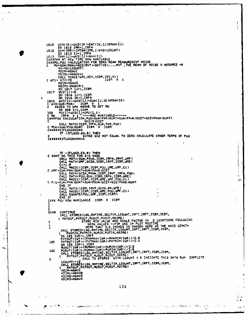
1915 &V3(IKI.UU3(rK?*EATCfl,IJ)Zt XA(IJ)DO 1812 IMR.1,IRFA

12E12 UV4(IfR).RNA(IMR,)D(LCOL4T)DO 1813 1J.1 IIRFA9 12~~I13 tXA(IJ).UU3(IJ)+WV4CIJ) .U TEMA FNIEVASMD4

CZ:ZPMU,PUIJ CALCU ATION FOR ZERO MEAN MEASUREN"T NOISEC MU.G*JA(MXA.)+CCZ(MIJT)#GCV(YDI....MTTEMA FNIEVASMDo

XI.YD(LCOUNT)NOZN.NSAUINDII1.SAUI4ICALL SCALE(UIICCV.ICBM,IRYXI)

C WMI1 G'^Y(YD ICBMf X 1KDiM-NSAV3NDIMi .NSAU3*1Do 1917 IJ.1.ICBM

1817 WU3(IJ).SDO0 1816 IJ.1.ICBN

aDO 1916 IK-1.IRFA1816 bV3(IJ).UV3(IJ)+GUA(IJ.fl911 XA(IK)C U'3*GUA(MXA) ICBM X IC ADDED TO WMI ABOVE TO GET MU

DO 329 I.1.ICBM329 MU(1 ).UU3(lI)*.'N(L 1)C MU IRFA X I ----- NOW AVAILABLE-----ClzPUU CALCULATIOP4.PUU-GUA(PXA )GUAT+GUA(PXUA )GCZT,6CZ(PXCUA)GUAT4C GCZ(R)GCZT

CALL MAT3(ICi. IRPA.GUA.PxA.PUU)C PUU.CUACPXA)GUAT ICBM X ICBMICzzxtIFLGCZZZZ:

IF CIFLGCZ.EO.E) THENC SINCE GCZ NOT EQUAL TO ZERO CALCULATE OTHER TERP.SOF PuUCttttttlPLGCZ~g:Izz

IF tIFLGSD.EQO) THENC DONT DO THIS FOR S-D CASE

CALL 9T C ,PUc~jFdfTg )CALL MAT4(UMF.GCZA.IC3MIRHTICPnDUME)

1 CALL MADDI(IC3M.ICBM,PUU.UMEUMFCt)C LPFr.CUA(PXA)GLI4T+GUA(PXUA)GCZ7

CALL MAT4(GCZA,PXVA,ICBN,IRHT.IRFA,PUUJ)CALL IMAT4(PUU,GUA,IC3M,IRFA,IC3M.UME)CALL MADD1(ICRDiIICBMWME.U19F,PUU,CI)

C P I-GJIA(PXA)CUAT4GUA(PXUA)GCZT.CC.ZCPUXA )WJATEND IFCA~LL ?AT3(ICBM,IRHT CCZA,RA.WME)CALL MADDI (ICBM. ICRf ,LMEPIJI.WMFCI)CALL EQUATE(PUU.MF,ICI ,.ICi)END IF

C912 PUU NOW AVAIL.ABLE ICBM X ICBM

CCSCOO CONrrNUE

CALL STORED(LGG.RN(TIME.D-LTI.LCOU1T.IRFT. IRFr.ICIM'. IC!M.

I FXOUT.PXTOUT.MUOST.PUO'JTNDIMSIC STORE MIN VAL.UE AND SCALE FACTOR IN4 2 LOCATIONS FOLLOL!IN:

c DATA VALUES --FOR USE IN PLOT ROUTINEC NOTE TH4AT 3.5 INCHES IS CHOSEN HERE AS THE AXIS LEMGTICALL STORED(LQ.R1TME.DELTIr,LCONMTIRFTIRFT,lCBM.ICBM

I F.XAiI,PXTh1.MUNl,pWriNNDIM6 IDO 12S IUR.1,IRFT!.XTOUIUR .MXAMAXCIWR)-XAMI(IUR))/3.S

15PXTOUTCIUR).CPXTMAXCILR)-PXTtIC1R))-3SDO 186 IUR-I,ICtMMU)OUT( IVE ).(IVAX(IUR)-MUMIH(IUR))/3.S

Bec PUOUTCIUR)aCpUmAxc IwR)-PMIN(IUlR'f3 .S

CALL STOREDLLOC RNTIME.,DELTIM,LCOUNT,IRFT,?RFT.ICDMZCDM,I NM(TOUT, PXTOU+ %UOUT PUOUT NDIMCI

C CALL O STOkED WITH LCOUNT C t INDICATE THIS DATA RUN COMPLCTELCOUNTO-I2 RTMETMLopTIF.RTIlCMCALL STORCD(LOO iT .CTPCUTIF.RTIDeCMI MEXTOUI .PXTOU+. MUOUT*PUOUT.NDIM6)

NDIMONSAV1

NDIMZ*NS*V3KDIM3*MSAV4

134

C RESET 10 TO SOME NONZERO VALUE TO AVOID TERMINATING THE PROGRAMC UHEN RETURNING TO MAIN ROUTINE, LOGRP

10-25END

tzECK MYPLOTSUBROUTINE. MYPLOTEND

IDECK AUCMATSUBROUTIHE AU AT(AA2,A3IFORMIRAICIA1,IRZ.ICAE)

C

:tTINDINE,"DIM3 MUST BE SET IN THEM CALLING POGRAM BEFORE USINGCz:lZNCIME.mDIM3 MUST BE SET Ih THE CALLING PROGRAM ?ErCRE USINGczzu;Z THIS SUERCUTINE. THEY MUST BE DECLARED IN A COMMON BLOCKC LABELED --MAIN4---C THIS SUBROUTINE FORMS AUGMENTED MATRICES OF THE FORMc IFORn-I A3-(A1 At)C IFORM-2 A3-(A1 A)TCCC IRAI.IRAZ°ARE ROJ DIMENSIONSIICAI,ICAZ,ARE COLUMN DIMENSIONS

DIMENSION AI(NDIM2.NDIR).Aa(MDIMZNDIMZ),A3(HD?3,h ] 3)CO"0 mrAlh4MD!M2.NDIM3IF (IFORM.E .'1) THEM

C FORM THE AUGMENTED MATRIX A3-(Al At)DO It Ii-1,IRAIDO 11 UI.I1oICA111 3(II°%Ij)-Aj(II1I1%)DO 12 IV-I.ICA2IVI- IV. ICA1

RETuRNEND IF

C FORM AUGMENTED MATRZX A3*(AI AR)TIRA3.IRA1.IRA2ICA3-ICAIDO 14 II-1.ICA3DO 13 IlI-oIRAL

13 A3(I1II):A11111,II)9DO 14 IU-,IRAE

IVIvIV IRA114 A3(I.UI.II).AB(IV..Il)

RETQCNEND

IDECK MVECIOSUBROUTINE MVECIO(A,NULMEL, IOKIN,KOUTNDIM)

C TRIS SUBROUTINE READS PRINTS ENTIRE (PORTIONS Or ) THE VECTOR

L A, DEPENDING ON THE VALUE OF ---10---. 3O-I---READ ONLYC IOB---READ AND PRINT, 10.3 READ SELECTED VALUE, 10%4

PEAD AND PRINT SELECTED VALUES1O----PRINT ONLY

C TO USE 10-3 OR A THE CASLLIN PROGRAM MUST IMITIALZE THE VEC.C rzzZTHIS ROUTINE SETS O0---- UHEN NO DATA IN ItiPUT FILECCREAD IS FROM UNIT SPECIFIED BY CALLING PROGRAM IN KIWURITE IS TOC. KCUT.HDIM IS THE DECLARED DIMENSION OF A IN THE CALLING

C FROGRAMCHARACTER MSCI6GDIMENSION A(MDIM)COMMON 'MAUNS' MSGIF (IOEO.I.OR.(IO.EG.2)) THEN

C READ ENTIRE VECTORIRITE(KOUTI)'ENTER ' NJMEL.'ELEMENTS)'READKINI.END-29)(At ),I2,NUMEL)END IFIF (IO0.C.1) THEMRETURNEND IFIF (IO.EO.3).OR.(IO.£E.4)) THN

C READ ONLY SELECTED ELEMEKTS. THE FIRST HJMER ON EACH CARD

C IS THE SURSCRIPT, THE SECOND IS THE DATA ENTRY

CI:%t:ZOH3TE ONLY ONE DATA ENTRY PER CARD

Cgz1z9Zt FIRST CARD MUST COTAIN THE TOTAL HJMSERR Or ENTRIES TO RE

C READ"RITE(KOUT#9),ENTER THE UIRER OF ENTRIES TO SE MADE)'

READ(KIN,%.ENDm2 9 )NUMEKT

DO e IT.1.NUMENT

URITE(KOUT.Z)'ENTEP THE ELEMENT NUMIER .THEM ITS VALUE)*

135

i i i •- l= _ . .. .. "

READ(KINz.END. )I.ENTRYA( ZJENTRYIF (IO.EQ.4)THENURITE(gOUT,33), ,,RITECKOUTz)MSGWRITE(KOUT.9)'ELENENT NUntBER * ENTRY)'URITE(gOUT, 11 )IA( 1)END IF

2e CO'*TrIhUERETrUP

IF ((IO.EO.a.OR.(IO.EO.S) THENC TO GET HERE 10-2 OR S SO PRINT OUT ENTIRE VECTOR

URITE(KOUT,33)'URITE(KOUToZf)RSGURITECKOUT,')' THE VECTOR HAS '.LIAEL, ' ELEMENTS'LR:TE(KOUT,2)(A(I)3.I-I,hUAEL)RETURNEND IFRETURN

29 PRINTZ."EMD OF DAT REACHED DURINM INPUT IN !MVECIO'

C ZZZ*% T+iS ROLUIWE SETS 10-6---- UHEN NO DATA IN IMPU! FILL33 ORmRAT cAje, ,o !FRRTZ, XII:'6

21 FORMAT(I4,L1X,12.6)

RETURWEND

IDECK NlAI0SUlPROUTINE MMATIR.C. I1C, N.KOU.NDI,.NDII'I)CHARACTER MS02SDIMENSION A NDIM,NDIMI)COMMON /MAUMS/ MSG

C THIS SUBROUTINE READS AND/OR PRINTS THE MATRIX A DEPENDING O THEC VALUE OF 10. IT READS FROM UNIT SFP'CIFZED BY KIN AND WRITES TO UN:TC gOUT. 10,1--READ EhIRE ARRAY 102--READ AND PRINT ENTIRECC ARRAY. 1O--3---READ SELECTED ELEM ENTS OF A ZO-4---READ ADC PRINT SELECTED ELEMENTS OF A 10S -- PRINT ENTIRE ARRAY1 UDII,NDINI ARE THE DIMENSIONS OF A IN THE CALLING PROGRAM

C :zZZZNOTE IF I'3 OR 4 THE CALLING PROGRAM MUST INITIALI2EC THE ENTIRE ARRAY BEFORE CALLC z:zttVrTHS ROUTINE SETS 10 -0 ---- UHEN THE INPUT FILE IS EMPTVC

IF ((IO.EQ.1).OR.(IO.EO.2)) THEMC READ ENTIRE ARRAY IN FREE FORATR0U MAJOR ORDER

URITE(KOUT,Z)'ENTER ',(IRZICI,' ARRAY ELEMERTS IN ROW RAJ ORDER>'READ(r INZ,ED.g9(A(IJ),J,1,IC),II, ,IR)-

END IFIF (IO.EQ.I) THENRETURNEND IFIF ((IO.EQ.3).OR.(ZI.EG.4)) THEM

C READ IN SELECTED ELEMENTS OF AC THE FIRST CARD I" THE INPUT STREAM RUST CONTAIN THE TOTAl.t NUMBER OF ELEIMENTS TO BE READ IN. ONLY OE ENTRY PER CARD.C TH4E FIRST ITEM ON EACH CARD IS THE ROW, THESECOND IS THE COL THEC LAST ON EACH CARD IS THE DATA FOR THA' '..CATIOMc FREE FORMAT IS USED

URITE(KOUT.)'EER T4E NUIQER OF ENTRIES TO IE MHADr.>"READ(K I.1.EhN-29 3UELDO 20 I-1,%UELUQITE(KOUTZ'ENTER THE RO.,AND COLLMNI FOLLOUED IV ITS VALUE)'READ(KIN.t.Etb2, ?Il.J.ENTRYA;II J),ENTRYIF (tO.EO.4) THENURITE(KOUT.33)'WRITE (gOUT,t )fSGURITE (KOUT 2)'(', II,' ',J, ),*CII.J)END IF

30 CONTINUERETURNEND IFIF ( IC.EO.2).OR.(1OEO.$)) THEN

C 10 • 2 OF S Ir HERE SO PPINT ENTIRE ARRAY

136

4.-.'

WRITE (K0UT, 33)'URITE(KOUT.Z )MSC9 URITE(KOUT.9)' MATRIX SIZE IS '.IR,' X( .ICDO 49 I-l,IR

49 WRFTE(OUT,4S )(A(I.J ),J.L.IC)33 FCRMAT(AIO./)

END IF

29 PRINT 1,'END OF DATA REACKI VjlN INPUT'C txz1zzrTH:.S ROU7INE SETS iG WwrN THE INPUT FILE IS EtiOTY

RETURNEUD

IDECK CLOGRSSUBROUTINE CLOGRS(GCSTRFM,MRFSSHM,GCX,GCY'.GCZ.1BCY.BCZ.FC,YD,RM,GM,FTRT,GTQT,RTHT. IRY. IFLGCZ.UMISV2,W,PO,GM.U4,UMSWMS,6

I UUI.UtJ2,UUUUXX.XO.UXU.U97.UIW)C THIS ROUTINE PERFORMS SET UP FOR USING THE CONTINUOUS TIMEC PERFORMANCE ANALYSIS FOR AMLOG REGULATOR

DIVENSIONGCSTRCNDIM.NDIfl),FMNDIS.NDIM).M(NDIM.DIl),PO(NDIM,INDIM.L"CNiDIM,ND)CCX(NDIMI.NOBIr.GYNDI.NtDIM).CZ(HDZP,tl~m).1 DCYgND IM. NDI),Z C NDIM,MD Il) )FC (ND IMMD IM, YD(NDI3).rlI (D:F.,

1 R(DIMDIM).T(DIM.NiDI),HTi(DI.D1M),V(NDtMI.W;FCir

I UXXNDIM,HDM).M4(ND,KDIM) wFM5("DIlNDIM)I UMstND!M,NDIM),.uXU(NDIM,NDIM,.Lfl ?CNDINDIM):WnuCNDrM,KDIM,DIMENSION COP1ICIl),COr 2(IiCHARACTER MSGZSSINTEGER IFLGCZREAL RKFSS(NDIM,NDIm)COMMON ,NAIM4/NDIM2,NDIM3

COMMON /MAUNSI' M'SGCOMMON 'MAINI' MDMMIIC~COMMON /KAIN2/ COM2COMMON .RNTIM'Rff7IME ,DELrzP!9 COMMON /IMOU/ KIN.OUTKPUNCHCOMMON /MAINE/ICBT.ICBMICFA.ICGA,ICGMICCTICGA.IRFAIRFM.IRFT,

, IPHT. IROA.IO,LQG. IRHM,MNft.DTSUkITE(KOUT.1)'DO YOU W~ANT TO CALCULATE EIGEHVALUES OF THE TRUTH MOiDEL AND CONiTROLLER MODEL F MiATRICES, Y OR m>,READ(bKIN.23.END-2933) MSG

23 FORMATCAI)IF CMSG.EO.'Y') THENWRITE(KOUTI) 'WRITE(KOUT,*ZVTHE EIGEIUALUES OF THE TRUTH MODEL F MATRIX'CALL MEIGMrF7.UVl,WV2oIRFTU~lI

URITE(KOUT.Z)'THE EIGENUALUES Or THE CDNT. MODEL F MATRIX,CALL MEIGM(FMUU1.WUE.IRFMW91)END IFCALL CKFT(FM.GM.RM,HM.KIiMDTS.RCFSS,QM,UM.M2W3.UM4WMS,WMG,I IRFM. IR4M, ICGM,GCV,GCZ.BM. ICSM)

c GCZ.GCY. IN GALL TO CKFTR ARE USED AS DUMMY ARRAYS FOR HE .F2CALL CDOMFMWXWUGSRIFcmwLWBW3u .WSW6

wRITEoKOL1T~t,h'ER THE TOTAL RUN TIME AND THE TIME INCREMENT>'IREAD(KIN.1 .EHD-293)RNT!ME. DELTIM

CALL IDK~T(IRFM.UMI.ClIC WMIfl~S IRFM X IRFM

CALL MATI(GCSTR.UMI.ICBM,IRFM.IPFMGCX)loesMSG. 'CCX FOLLOWS, OCY,GCZ SET60'CALL MMATIOCCCX ICBM IRFM IO.KIN,KOJ7..NDIrMNDIM)

C NOTE229212 OTHER GAIN MATRICkS.GCZ.AND GC SHOULD BE CALCULATED INC THIS MODULE FOR USE IN THE PERFORMANCE ANALYSIS ROUTINE.

Do 2962 IIZ.1ICIM

DO292902..IHIFLGCZIl-PE NLSS OTN SSI

C IFLOCZ, I INDICATES GCZ 19 SET To ZERO--RFAAYI OTN SSI

9 Do 2903 1011602soYD(I)*e

137

IRY-IDO 1723 Z.I.ICBMDO 1723 J*1.IRy

1723 GCY(I.J)-oC FORM SCY

DO 178a 1-1.IRFMDO 1702 J-l.IRY

C YD IS ALLOiWED TO ONLY BE A SCALAR AT THIS TIMEC FORMBCZ

CALL iGUATEBDCZ.RKFSS,IRFMIR4r)MSG.'RCZ FOLLOUS,BCY.S'CALL MMATIO(SCZ. tRF,IR1.I,oIN.ourt.NDiM,Di ,

C FORM FCCALL MATI(BMGSXIRFM,ICB.IRFM,UMI)CALL MADDI(IRFM.IRFMFM,UMI.,Lt2.Cl)LRITE(KOUT.2),UP.ITE(KOUT.:,'DO YOU WANT TO CALCULATE THE EIGENVALUES OF THE CONTIIUOUS-TIME LO CONTROLLER? V OR to'READ(KIN.23 )MSGIF (MSG.EO.Y' ) THEN

WRITE (KOUT,I~oT4E EIGENVALUES TH4AT CORRESPOND TO TH4E POLES 09I THE COKTINUOUS-TIME LO CONTROLLER ARE...

CALL MEIC(WU,U1.UU2,IRMLJMI)END IF

CALL MAT1':RbFS,HM IRFM.IRHM.IRFMWMI)WRITEC(ZOUT.Z.1'WRITE (KOUT, 9'IDO YOU WANT TO CALCULATE THE POLES Or THE CONTINU

IOUS-TIME KALMA4 FILTER? Y~ OR N)'READ(I.23 )ISGIF(MSG.EG. 'V') THENCALL ViADDI CIRFM. IRFMFM,WMI1 UM7,Cl)URITE(KOUT,*)'THE EZOENVALUES THAT ARE THE POLES OF THE CNOTINU

IOU$-TIME KALMAN FILTER ARE....'CALL EINh(UM7,UVI.UVa,IRFM.UM8)

END IFCALL M'AD(IRFI,IRFM,UM2,UM1.FC.C1)MS5G*' FC FOR THE LOG CONTORLLER IS'CALL MMATIO(FC. IRFP1DIRFM,IO.KINKOUTNDIPINDrm)URITE(KOUT~t)'URITE(KOLJT,Z)'DO YOU WISH TO CALCULATE THE EIGENVALUIES OF THE LO-. -

9ICONTROLLER F MATRIX9 Y OR N),REP4D(IM,23 )M'SG1 IF (MSG.EO.'Y') THENWR'ITE(IZOUT,S)'URITE(KOUT,Z)'TNE EIGENVALUES OF THE LOG CONTROLLER F MATRIX ARE'CALL MEIGN(FC.1JU1.UU2.IRFM,LMI)END IFRETURN

2933 10-0END

* ZDECK DASISUBROUITINE DASI(GOT.RM..CB.1M3.I.RFM)DIMENSION GOCTfNDIM.NDIM),3!i(ND1MNDIN),U(nlIMNDIM).

I W3(NDIM,?DlM).COM~1C),COM~tI)c THIS SUBROUTINE MODIFIES GQGT AND RETURNS THE MODIFIEDC VALUE IN GOOT. WHERE COOT IS USED IN THE KALMAN FILTERC GAIN CALCULATIONS. THE MODS ARE IN ACCORDANCE WITH THEC THE TECHNIQUE DEVELOPED BY DOYLE AMD STEIN IPI OROBUSTNESSC WITH ONSERVERS'.IEEE TRANS. ON AUTO. CotITROL.UOIL A024,C NO. 4,AUC. 79.PGS 607-611-CC THE VALUE RETURNED IN Q=OT IS 00 . HERE 00 ISC OOvOOGT+SQCSG~vMCV~lMT)CC 50 15 A SCALAR DESIGN PARAMETER THAT AS 1T APPROACHESc INFINITy. CAUSES THE LOG CONTR6LLER TO RECOVER THE ROBUSTNESSC PROPERTIES OF A FULL STATE FEEDBACK CONTRCLLER.CTHE MATROX--V-- IS ALSO A DESIGN* PARAMETER WITH THE RE0UIREPENTC THAT IT BE POSITIVE DEFINITE. 3M---- IS THE CONTROLLER PrODEL INPUTC MATRIX. C04T --- IS THE CONTROLLER MODEL ImouT NOISE STRENGTHC MATRIX OM PREMULTIPIED By GM AND POST MUTIPLIED BY GMT WHERE GM ISC THE INPU+ NOIESE MATRIX.

CHARACTER MS50160COMMON ,MAIKI/NDIMNDI 1.COMICOMON /MtAIN2/ COM2COMMON /INOU' KIN.KO4JT,XPUNCHCOMMON /mAUNS/ MSGURITE(KOUT,11)'URITE(KOUTt)'THIS ROUTINE MODIFIES THE VALUE OF OMfOM)CMT

I USED Ihi CALCULATING THE KALMAN FILTER GAIN, RKFSS.'WRITE(KOUT.1)'THE MODIFIED 0 IS v GMCOM)GTSOIIBV~t~iWT)HRE

138

10

I SO 1S A SCALAR DESIGN PARA9ETER-AND V IS A POS!TIVE DEFINIITEIliATRIX rESIGN PARAM~ETER. THrE LARGE-R Soo THE MORE ROBUST THE CONTROIL. SYSTEM~ UIL. BE.'

p 9 DO 5 IMPI,iS0BUPRTE(KOUT.41),

11 FORMAT.:Aie,/)WRlTE(KOUT.t)'EMTER I-To INPUT so, 2-TO INPUT U 3- TOCALCUt.ATE M'OD

IIFIED 0, -4- TO EXIT THIS ROUTINE>'READ(KIMZIz)ISEI.GO TO (1.2,3,4)ISEL

I URITE(KOUT.11)'URITE(Y.OUT,%)'ENTER SQ)e--)'READ(IKIN,Z )SOGO TO 5

a RITE(KOUJT.Z1)'WRITE (KOVT.t)'J IS INIALIZED TO .ZERO UPON ENTRY INTO THIS OPTIO

IN.DO 7 I*1,NDIM

* DO 7 J1%,KDIM7V(X.J)-e

WRITE JKOUT, t)'ENTrER I.0 OPTION FOR POSITIVE DEF V(SEE INPUT ROUTIN

READ(K!N :)I0MSG.'DESNON PARAMETER V MATRIX ENTRIES'CALL MM-ATIO+UIC;1 CBM.bO.KIN.KO(T.ZM.NDZM)

a dALL M4T3UlRF.IRFMBM ,U,3)C ij3.BMtV)p ", 1RFM X 1RPM

CALL MADD1(IRrM,IRFM,COCTL? 3,V,501)C V IRFM X IRPM HOU CONTAINS THE MOD. VALUE --- 00

MSG-'THE DOYLE A4D STEIN MCDIFED 00 MATRIX IS'IO*5CALL MMATIO(U,IRFM,IRFM,IO.,ZIN,KOUTNDrM,NDIM)

S CONTINUE4 CONTINUEC 00 IS ACCEPTABLE SO PUT INTO GOGT

DO 20 II,IRFMDO U0 J*41,IRFM

2e GQ^STCIoJ).UcI.j)RETURN9 END

IDECK "YINTGSUBROJ'rINE MYINTOPMIITA,TBA6.Er,GA,0AFABA.IRFAICGArRY,I IROQI)_'

C THIS SUBROUTINE SETS UP THE NECESSARY~ INTEGRALS FOR USE ByC THE PERFORMANCE ANAL. ROUTINE. THE STATE TRANSITION MATRIX.c 'EXP(FAtTI1 E)aEATo INTEC(EAT(GA, OA (GAT) EATT), AND

-C PITEG(EAT (RAJ). UI E IS A DLqqlY WORK SPACEREAL PHI (NDIZ.NDIM2) ZKTCACND1n2,NDI.2).INTBA(?tDIM2.NDIMe)

IGA(NDIM2,NDIMa),FA(N~lI-2.DIM2 )

DIMENSION 0OmjcI),COm2cI)COM'ON/MAIN1/NDIM.NDIM1 ,C"MCOM'OK/MAINo' COMPCOMMON /IKOU' Kt~i,KOUT,tKPUm:HCOM04 /'RNTIA-.RHTIM, bLTIMCOMMON /MAIN4^.NIM2.MDIM3

rcxr.FORM QA(OA)GAT --NEED FOR KLIEHMAN ROUTINEC

NSAJI NDJIqNSAIJ2.NDIMINDIM&NDIM2

CALL DSCRT(IR7A,FA,DELTIM,INTGA,UME,le)C UPIE-INT(EAT)

CALL MATI(UME,BA IRFA.IRFA.IRINTBA)C INTBA. INT(EAT)DA iRFA XIRY NEEDED IN MXA UPDATE

CALL MAT3(IRFA,IR0A,C*,OAPHI)C PHIGAC0A)(GATI IRFA X rRFA

CALL INTEG(IRFA,FAD PHI. INTGA,DELTIM)C PHItEXPCFA) IRFA X IRFAC JKTOA-IN-EGAAL C EXP(FA)(GA)(OA)(GATT)(EXP(FA)7)) IRFA X IRFAC

ND !M-NSAVINDIMI.NSAV2RETURNEND

13P

%DECKC DSCRTZSUEROUYTINE DSCRTZCUMl.PHINIRDYD,3CZD1RNDELT1M.FC.,CY.

I IRY.DCZIRHI .PHIT,OTD,3TD,CT,0T.Fl.3T,IRFT,ICGT.ICBT.IRNT.IRTO,PTCCX, ICFM)

C THIS. ROUTINE DISCRTIZES A CONTINUOUS TIME LQ^ CONTROLLER U'SINGC FIRST ORDER APRROXIMATIOMS TO THE REQUIREC INTEGRALSC AND PROVIDES A!4 EQUIVAL.ENT DISCRETE TIME REPRESENTATION OF THE TF>J7HC MODEL FOR USE IN THE PERFAL ROUTINE

REALVM I.CNDIM.?1DIM),PHIM CtDII'INDI7.),BCYD CNDII9.NDIN).I BCZD(HD!It.NDIM).FC(NDIM.NDIi), RC%'(NDIM.NDIM),I DC2(MDIMND),PHIT(DrNDI),OTD(NDIi.NDIM).I BTD(NDIM.HiDIM),CT(NDIM,DI).T(DI,DI).,I FT(NDIM.MDIN), lT(NDIM,NDIM').RTD CtDIM,NDIN),I GCX(hDIM.NDIM,RT(DIN.NDIM)REAL COMI1(l),COtKtCI)CH4ARACTER MS02ICOMM0K/iAIhI1.'DIP,MDIN1.CONICOMMOtVNAIt48/ COM2COMMON'NAIh4'NDIME. NDIM3COM90I - INOU/KI N.KOLrT ,PUHCH

CALL IDKTCIRFR.UMiI.Cl)CALL rDRTCIRFN.UP!I.CI)CALL MADDI(IRFM rRFM U'.FC,PHIM DELTIM)

C PHIM I#FC(DELTI1 ) 14T ORDER APPROX T6 STATE TRANS MATRIX OF CONTC CALCULATE OW --CTR

CI.-'.eC RECALL THAT GCSTR LIAS PASSED INTO THIS ROUTINE IN BTO

CALL SCALE(GCX. ETD.ZCD(. ZRFFM,Cl

CALL SCALERSCYD, ICY, IRFM. IRYDELTIM.)B CYD DISCRETE TIME APPROX OF BCY

CALL SCALE CBCZD, BCZ, IRFMI RHMDELTIM)C CZD DISCRETE TIME APPROX OF ICZ

hSAV3-NDIM2NDIM'2.NDIMCALL MYINTGCPHIT.OTD,BTD,.INIGT,QTFT.DT.IRFT,ICCTICIT,ZRHT)NDIPI2-MSAV3

C PHIT,QTD,BTD ARE EOUIV. DISCRETE TIME REPRESTATIONS OF TRUTrH MODLC PATRICE

VRlTECKOUTr,:)'URITECKOLIT,*)' WAS THE VALUE ENTERED IN RT DURING INPUT A CONTINUIOIUS TIME OR A DISCRETE TIME VALUE? ENTER A C FOR CONTINUOUS *AI D- FOR DISCRETE VALUE)'READ(KIH. 12 )MSG

12 FORMATCAI)IF (PSG.EQ.'C') THENCI.I/DELTIMCALL SCALE(RTD.RT,IRHT.IRH4T.CI)ELSECALL EQUATECRTDRT. IRH?. IRtT)END IF

C RTD IS THE DISCRETE TIME APPROX OF RT

CALL IDMTCIRFT.UNI*CI)C W'~1-GTD - I

ENDIDEcC DLOORS

SUBROUTINE DLOGRSCGCX.CV.OCZ BOY BCZ,PHIT.PHICRTD,GTD OTO,I BTD FM,lM 019,GM RNNA CT.o- OT . t .3.RT.HTUXX.UUU.GCSTR.ArFSS.,'D.I IRY:IF1.GCi.UXU. UMI. ~UMU3,1JM4.wsUME.IUV)

CTHIS SUBROUTINE FORPATS THE SAMPL ,ED DATA CONTROLLER INTO THE FORISATC REQUIRED 3%Y THE PERFORMANCE ANALYSIS ROUTINEC THE FORMAT Is SPECIFIED Ih THE COMMENT STATEMENTS IN THE CODE. AhDC IN-MORE DETAIL IN E. LLOYD S MASTERS THESIS.DBI.AFIT.

REAL COMiI(l),COM2(1) NI) C(DMNI)REAL GcX(NDIM,NDZM),CyNDIM.D~GCNDMNI)

IDCYNDI.NDM).BCZNDIM.NDIlA).PHI, (NDIMi.NDfM).I PHIC(NDIM,NDIM),RTD(NDIMNDIM),GTD(NDIMNDIM).lOTDCMDIMMDIM),RTD ( DIfl,NDIM),FM(NDIM,NDIM),1 DflCNDIN,KDII ), OM(NDIM,hDlfl),GCI(NDIM.NDIM),I UVl(NDIl),tJI2CNDIM)p-1 ("4 DIM, NDIN), MMCNDIM, NDIM),CT CNDIM, NDIM),IOT(MDIM.NDIM), FT(NDIM,NDIM), ST(NDIM,HDIM),IRT(KDIMNtDIM,TNIN,NDI).XXCD:MDI),I UUU(NDIN ,NDIM),.GCSTR(NDIM NOIM), RKFSS(NDItiNDZN).I Uxu(NDIN..ND1IN),UNI (NDIMNNIR).Ur2CNDIM,MDIM).i UP,3 CDI,MDIM).UM4(N4DINNDIM).UM(NDIM,MDIM)9 PEAL YDCNDlr3)

INTEGER IFLGCZ

140

CHARACTERqsozse msciZi ,msG2Z19COWWnO /AI/?DIM.NDlt~1.COM1

COMMiON /MAIN2/COK2C0MlOh/Th0U/KIH, iOUT, KPtJCHCOMMON .MAlh4/HDIM2,MDlfM3

*1 COMMO1N/"AUNS/MSGCOMMON /RNTIMi'RNTIME. DELTIMCOM4M/MAIMG/IC!T, ICBl, ICFA, ICGAD ICCM. ICGTD ICQA.IRFA. IRFNq. IAF,

I IRHT.IROA.IO.L0C.IRHM.NUMDTSWRITE(KOUT,S:'EMTER THE TOTAL RUN TIME AND TrHE SAMPLE TIME)'READ(KIN.X )RNTIME,DELTIM

11 FORMAT(AI)C CALCULATE EQUIVALENT DISCRETE TIME VERSIONS OF, N-N.G-GDIC ON--Q'(D. AND PHI" THE STATE TRANSITION MATRIX FOR FM

C SINCE WORKSPACE IS AT A PREMIUM , THE TRUTH MAODEL MATRICESCPMIT.RTD,GTD,GTD,RTD WILL RE USED FOR THEIR CONTROLLER MODELC COUNTER PARTS DURING THIS ROUTINE SEFORE THE EQUIVALENT DZSCRETEC TIME TRUTH MODEL IS COMPUTED. AT THAT TIME THERE IS NO LONGEG ANYC NEED FOR THOSE CONTROLLER MODEL MATRICE SINCE THE CONTROLLER 1S PUTC INTO THE PERFOMANSCE ANALYSIS FORMAT.PHIC ICY .. CCZ

NSAU3-ND4M2ND IM2-NDIMCALL MYINTG(PHIT.CTD,BTD,RTD,GM,OM,FM,BM,IRFM.ICGNDICBMDICGM)

C RTD IS USED AS DUMMIY WORK SPACE IN CALL TO MYINTGNDlr.2.NsAv3CALL IDNTCIRFMGTD..CeeWRITE(KOJT,Z)'ENTER A C IF THE VALUED ENTERED AMID RM IS A CONTIMIUOUS TIME VALUE TO FORM THE BASIS OF AN APPROXlMATE DISCRETE TIME1 RM,EMTER A D OTHERWISE),READ(KINI . )MSGIIF CMSQI.EO.'C'3 THEN

C APPROXIMATE R1 D-Rl/SAMPLE TIMECI * /DELTIMCALL SCA.EtRTDRMIRHM.IRHM,CL)ELSE

C THE VALUE IN RfY IS DISCRETE TIMIE ALREADY* CALL EQUATE(RTD.RV .IRHMIRH19)

END IFC SET UP-X , S , AND U FOR DDTCON

CALL XSU(GCZ,GCY,PHIC,GCX, DCY, CZ,RKFSS,UM.uW 2,U1'3, UM4.UMS,I FM,BM,IRF"MiICIm.uxx,6.Wu.xu,PHIT)

C GCZ NOW CONTAINS X. PHIC CONTAINS U.GCY CONTAINS SC GCXRCZ,tCY,RKFSS WERE DUMMY WORK AREAS IN XSU

CALL DDTCONCPHIT,Wxx.CCX.GC.TD,P4IC.RKFSS.ICV.C.GC.AL.1 GCSTR.XUWMI,UM2.UN3.WM4mVM5)

CsCY.BCZ GCYPHIC.GCZGCX,RCFSS ARE USED AS DUMM1'Y WORK SPACE I" DDTCONURiTE(KOIT,*)'DO YOU WISH To COMPUTE THE KALMAO( FILTER GAIN OR PIC1K IT DIRECTLY (AS IN MAYBECK SECTION. 14.S)EMTEW A C TO COMPUTE EINTER A P TO PICK IT DIRECTLY>'READ (KIN.II)RSCZIF (MtS4Z.EG.'C')THlENCALL DKFTRtPHIT.BTD.GTDOTD.GCX.RTD.WM.CCY.GCZ.P4IC.RKFSS.RCY.ICZ.

CG.Cx,GCY,GCZ.DCZBCY ARE USED AS DUMMY WORK SPACE IN CALL TO DKFTRELSECALL PKDIRC(CCX.PHIT.GCY,GCZ HM STD.RKFSU.ICBMIRFM.IZRHM)

C GCX,GCy GCZ ARE, DLjf Y UORKSPACjS IN CALL TO PKDIRCEND IF

Crtattz:zztt*INTHE FOLLOWING CALCULATIONS. ICYGCY,3CZ ARE DUMMY UORKSPCz*ssz*%IZUACES UNTIL THEIR LAST USE WHEN THEY ARE SET EQUAL TO THEIR FCttttStZZiAL VALUES FOR PERFAL SUBROUTINE

CALL IDNT(IRFM.ICY.CI)CALL MATI(RKFSS.NMIRFM.IRHM.IRFM.GCY)

CALL MADDI(IRFM,IRFM,RCY,GCY.ICZ,Cl)C BCZ aI-RKFSS(HM)

URITE(KOU'T.2)"'WRITE(KOUT,%)'DO YOU WISH TO CALCULATE THE SAMPLED-DATA FILTER P

IOLES7 Y OR N>'READ(KIN,12)MSOIF (msG.EQ.'Y') THENCALL MATI(PHIT,vCZ,IRFM,IRFM IRFM PHIC)WPITE(KOUT,S i'THE EI6ENVALUES THA+ CORRESPOND TO THE SAMPLED-DATA

1 FILTER POLES ARE..

14 1

CALL MEIGNCPIIIC,UVI.UVZ.IRFM.UMI?END IF

CALL SCALE(RCYDGCSTRXCM.RF',Cl)C SCY--GCSTR ' ICII! X 1RFM

IF (flSG2.EG.'C') THENC FORMULATE THE OOTIMAL CONTROL LAU FOR PERFAL

CALL MATI(BCY,BCZ.ICBI ,IRFM,IRPM,GCX)C GCX- -GCSTR(I-RKFSS(HM)) ICili X IFRM

CALL MAT1(2CY.RKFSS.XCDM,IRFM.IRHM.GCZ)C GCZ- -GCSTR(RIFSS) ICBM X IRHMt

IFLGCZ.*CALL MATI(BTD.Y.IRM,ICI'.IRFM.CCSTR)C1.1.0CALL MADDI(IRFM,IRFMPHITGCSTR.DCY.CI)

C RCY- PIIT-STD(GCTR) IRFM X IRFMURITE(KOUT.Z) 'URITECKOUT.R)'D; YOU UISH TO CALCULATE THE POLES OF THE OPTIMAL

I LO SAMPLED-DATA CONTROLLER? Y OR N>1READ(KIN 12)MSGIF CMSG.tQ.'Y'i THENURITE(K4OUT Z1-'THE EXCENVALUES THAT CORRESPOND TO THE POLES OF TH

LE OPTIMAL CC CONTROLLER ARE .........CALL MEIGH(BCY.6%IJ.WVE,IRFMPHIC)END IF

CALL MATI(ICY,BCZ,IRVM.!RFM.IRFMPH!C)C PHIC .(PHIT-9TDLGCSTR)tl-RFSS(i9)) IRFM X IRFM

CALL MATI(BCY.RKFSS,IRFM.IRFM,IRHMBCZ)C BCZ.(PHIT-ITD(GC^STR))RKFSS IRPM X IRHM

ELSEC FORMULATE THE SUBOPTIMAL CONTROL LAUD UST--GCSTR(X AT TSUI I MIINUS)

CALL EQUATE(GCX,DCY.ICRM.IRFM)C CCX--GCSTR ICBM X 1RFM

CALL I9ATI (PHITBCZ, IRFM, 1RFM, IRF7 ,GCSTR)

CALL tATI(ITD.GCX,IRFM,IC3MIRFM,3CY)LRITF(KOUT,2)'URITE(KOUT.2)'DO YOU WIISH TO CALCULATE THE POLES OF THE OPTIMA

IL LQ SAMPLED DATA CONTROLLER? Y OR N>1READ(KIN. 12 diSCIF'UiSG.EO.*') THENCALL PADD1(IRP".IRFM.PHIT,tCY,PHIC.CI)

URITECKOUIT,I)T4E EIGENVALUES THAT CORRESPOND TO THE POLES OF THE1OPTIMAL LO CONTROLLER ARE ... I

CALL MEIGN(PHIC,UUIPUU2. IRFI9,WMIEND IFCALL MADDICIRFM.IRF',GCSTR,DCY,PHIC,CI)

C PHIC- PHIT(I-RKFSS(Ifl))-BTDGCSTR IRFM X IRFMCALL MAT1(PHIT.RKFSS,RFM.IRFi.IR4M.3C2)

C BCZ-PHIT(RKFSS) 1RFM X 1R149DO 101 1-..RFMDO lSLJ.1.IRHfl

lot GCZ(I J)-eIFLOWi.END IFIRY*IDO 102 1*II4DIMDO 102 J.I.IRYcCYCIJ)w*

le 10 ICYCZ.J~fDO 107 I,1,1666

167 YDCI).*

MSa.'PHIC FOR THE SAMPLED DATA CONTROLLER 161CALL MMATIO(PHIC,IRM,IRFMi.10,KIM,KOUTNDIM.NDIMDURITE(KOUT.Z)'URITE(KOUT,Z)IDO YOU UAMT TO CALCULATE THE CICENUALUES OF THE LOG1 CONTROLLER STATE TRANSITION MATRIX, PI1C? V OR M>'READ(KI4, 12 )MSGIF (MSG.EC.'V') THENM FTELCCNROLRSAETASTWRITE(KOUT*9)'THE EIGENVAUESOTILOCORLLRTAETAITION MATRIX ARE..CALL HEIGN(PH1CWJ.U,I~RPM.UMI)

K 142

END IFPMSG*DBCZ FOLLOWS, RCYS6'9CALL MMTOIZIF.RM1 IOTKlDEMSG-lGCX FOR THE SAMPLED DATA CONTROLLER is,CALL MAT1O(GCX,ICBM.IRFf.IO.ZIN.OUT,HD.NDXM)IF t(SG2.E9.'C') THENMSG*IGC7, FOR A COMPUTED KFSS'ELSEIS'GCZ FOR KFSS PICKED DIRECTLY'END IFCALL MATOGZIBRM10KMK~tMI.DMWRITE(KOUT,Z)' CCY IS SET w 9

C THIS IS A REGULATOR SO YiD IS ALWAYS ZERONSAV3.NDIM2HDIMZ *NDIMCALL MYINTGCPHITOiTD,STD.RTD.GToOT.FT.UT.IRFT,1CCT.ICBT,IRHT)

C RTD IS USED AS DUM9Y WORK SPACE IN CAL TO MIITGHDJM2*NSAJ3

C PHIT,QTD,BTD ARE EQUIV. DISCRETE TIME REPRESTATIONS OF TRUTH MODLC IqATRICE

WRITE IKOUT.Z)'WRIECKOUT,Z)' WAS THE VALUE ENTERED IN RT DURING INPUT A CO~fT1NUO1US TIME OIL A DISCRETE TIME VALUE? ENTER A C FOR CONTINUOUS,1 D FOR DISCRETE VALUE>'READ(KIN "12)MSO

1e FORMATCA1)IF (MSC.EO.'C') THENCiI/DELTIMCALL SCALECRTD,RT,IRIT.IRHTCS)ELSECALL EQUATECRTD.RTIRHT.IRHT)END IF

C RrD 1S THE DISCRETE TIM E APPROY OF RTC1* 1.6CALL IDNTCIRFT,GTDoCI)

C GD GTD IRETURNEND

tDZECK FTSUBROUTINE DKFTRCPHIM,3MD.GMD,OMD,UWI1,RMD.HM.WI3,UMSWM6,RKFSS.I F2,H2oF",GVn.OM,3M.WMZ,UM4)

C THIS ROUTINE CALCULATE THE STEADY STATE KALMiAN FILTER GAIN P.ATRIXC FOR A SAMPLED ATA CONTROLLER

REAL PHIM(NDIM,MDIDHDIMNDMXM),MDNDI,Dl),I GMD(NDIM.NDIr,UMCNDIMHDIM).RDDr.,nDIM4.I HM(NDIM,MDIM), UM3(MDIM,MDIM5, UMS(NDIMAtDIM..I UM6(MDIM.NDIM), RKFSSNDI ,NDIM),F2NDIMi.NDIM)I ,H2(MDIMDIM,FM(DIM,MDIM).I G1A(DII,NDIM,OM(DII,NDIM),19(NDIMNDIM),I hrn2cNDIM,NDIgq),u94cNDIf ,ZIM)

REAL COI'I(t),comaCI)CO PIOH /MAINI"INDIMIIDIMX.COMICOMMONt elHOU1 K1N.KOUT KPUtNCsCOMM"t .'Rt4TIMx RkTInqE fELTIMC0MOhMAI4,N"DIM.HNlMCOPWI"Ul4.-MScCOM~MON *MIM~I2/ COMg

COMMON -MAX N6/1CRT. ICBM. ICFA. ICA. IMICTICOAIRFAIRFIR.T,I lRHT.IROA.1O.LG.RHM.NUmIDSCHARACTER MSGltl .PIsO:e6

C DELETE DETERMINISTIC STATES AS IN THE CONTINUOUS TIME CASEwRZE(eCou7.,'zp YOU PLAN TO USE THE DOYLE AND STEIN TECH4IQUE FORI THIS RLR' YU MAY WISH TO MODIFY THE VALUE OF NUMDTS, THE NLR9IER0

IF DETERMINISTIC STATES. DO YOU WANT TO CHANGE NUt DTS7 I'O )READ(KIN.II )MSC1 R oNUMsAU.NUUiDTsIF (MSOI.Ea.'' THENURrTE(KOUT,&)'ENTER THE NEW VALUE OF kUlCTS FOR THIS RUN>'READ(KIM.a )NUMDTSEND IFIRITE(KOUT.:3'NUMDTSe '.NUM9DTSIDS-NU'DTS~lIRFe. IRFM-HUMDTS* IF(NU19DTS.EO.,) THEM

143

C STORE SYSTEM MODEL IN INTERMEDIATE MATRICES comPAibDLEC WITH THOSE BELOW WHEN THER ARE DETERMINISTIC STATES REMOVUEDCALL EQUATE(F2,PHIM.IRP2,IQFZ)

CALL EGUATEUN1DGD.IRF2.IRF2)CALLkEQUATE(H219, IRsM. IRF2 ICALL EOUATE(VMS,1MD. IRF2. ICBM)CALL EQUATECUPI2.OMD. 1RF2. IRF2)ELSE

C DELETE THE DETERMINISTIC STATES FORM THE MODEL USED TO FORM~C THE STEADY STATE KALMA4 FILTER GAIN MATRIX

DO 2112 I*IDS.IRFM1I-I-tiUMDTSDO 2112 .r*DSIRFMJJ-J-NU DTS

2112 UMi4(II.JJ).FMq(I,J)DO 2113 I"1.IRW4DO 2113 J*IDS.IRFMJJ*J-NIJMDTS

C FOR" 12D G2D NOUDO a1l5 I-IDS.IRFMII .1=tIUIDTS-DO a1ils Jol.ICDM

9116 UM3'11.J):BM(I J)Do 2114 1I..DSRFMII-NJMDTSDo 2114 Jol.ICGM

2114 Vft 1I.J)-GM(IC.J)11 - FORMAT(Al)

NSAU*NDIMBNDIfi24NDI'CALL YINTGCF2.UM2,UMS.WMS,UM.QM.UJM4.UM3.IRF2,ICGM,ICM.ICM)NDIfl2.NSAVcl-I.,CALL IDNT(IRF2,UMI,Cl)END IF

C CALCULATE GMD (CMD) GFW?9 CALL HAT3(IRF2.ZRF2.MlUM.RCFSS)CRKFSS IS DUMMY WORK SPACE AT THIS POINT IN THE PROGRAM

-URITE(KOUT,:)' DO YOU U1514 TO MODIFY THE 0911 MATRIX BY THE DOYLE.AND STEIN TECHNIGUE FOR CONTINUOUS TIME CONTRCLLERS EXTENDED TOITHE DISCRETE TIME SYSTMS, Y OR N)'READ(KI)1.11 )MSCIIF (ISGI.EG.'Y') THENCALL DAS2(lM,RKFSS.UM1,ICBM.Ur3.IRF2.UM6)

C RETURNS A M~ODIFIED ORD VALUE To BE USED IN FINDING RKFSSEND IF

C CALCULATE THE KALMAN FILTER GAINS, RKFSS# FOR-EITHER THE MODIFIEDC ORD OR THE UNMODIFIED ORDC ORD IS STORED IN RKFSS

CALL TRAfIS2 IRH1M, RF2j'2*UM3)CALL KFLTR(IRF2,IRHMF2U3,RFSS.RD,rnUrI,UMS)

C 64 msPISS,UWqS CLOSED LOOP MEAS MATRIXC UMI a RIZFSS UITHOUT THE ZEROS FOR THE DETERMINISTIC STATESC NiOU ADD THE ZEROS FOR THOSE STATES

IF CNUMDTS.EQ.0)TH1EDO 2929 1-1 IRFM

mg9 RKFSS(I.J'UUM1(1,J)ELSEDO0 2119 J.1,IR1'DO 21121I NUMDTS

2110 :KFSS(I,4)'*DO 2119 I*IDS.ZRFMI1.I-NUMDTS

2119 RKFSSI.JI'hlMlCII.J)END IF

C NOU WRITE OUT THE RKFSS MATRIXelf 10-5

PSG-'STEADY STATE SAMPLED DATA KALM44 FILTER GATN MTRIX,CALL MATIO(RKFSS.IRFM,IRM.IOKIN.KOUT,NDIM,M,MhMPDTSmNUI SAVRETURNEND

tDECZ DAS2SUBROUTINE DAS2(IM,0MD,UIClM.U?,3.1IRN,W'i)REAL IM(NDIM.NDIM.QGMD(NDIM.NDIM). IJCNZIM.NDIM).

144

* C THIS ROUTINE ALLOWS GIC TO BE MCDIFIED IN A MANKER SNMILAR TO THE D3C YLE AMC STEIN TECHNIOUE FOR CONTINUOUS TIM SYSTErS.'C G"DM~OL,.QND +SQzSO)(?CU()RMT)*SAPLE TIMEC W- ERE SO iS A SCALAR DESIGN PARPIETER AMD V IS A POSITIVE DEF:NITEC SYMETRICM.ATRIX DESIGN PARAMETER. AS SO --- >TO INFINITY IN THE COC KTINU0US TIM'E CASE, ROBUSTNrSS PROPERTIES Or A FULL STATE FEEDBACKC CONTPOLLER ARE RECOVERED. iHIS ROUTINE IS 'BASED ON E. LLOYDS MASTERSC THESIS .DEI, AFIT

CHARACTER FMSG16eREAL COP 1(1,COP2(l)COMMOQN /PAI/NDIM.NDIMI.COS1COMMON /RTI.'RTIE..DELTIMCOMMON /KAUNS/P9SCCOMMON /MAIK2/ CoraCOO,"ON /IKOU/ZIN.KO!T.KPIJNCH

11 FORMAT(AI)WRITE(trOUTZ)'THIS ROUTINE MODIFIES THE VALUE OF O1C USED TO CcALCUILATE TH4E STEADY STATE KALMtAN FILTER GAIN. THE MODIFICATION PERFORIMED IS SIMILAR TO THE DOYLE AND STEIN TEC$4NIQUE FOR CONTIftUOUS-TIMIE SYMM~fS. FOR A COM9PLETE DESCRIPTION SEE E. LLOYDS MASTERS THES:is. AF LT, vSI. tR:EFLV THE MODIFICATION ATTEMPTS TO ENHANCE ROVLS?hiESS OF THE LOG CONTROLLER AND IS OMDGLQDCDTStQDL'rI ZcBN(U)tfMT))... THE LARGER THE VALUE CHOSEN FOR THE SCALAR SO Ti.IE MORE ROBUSTNESS RECOVERY (CO MPARED TO FULLSTATE FEED-1ACK), V KLUST BE A POSITIVE DEF. MATRIX, CHOOSING V-1 ADDS PSEUDONOISE EQJAILLY TO ALL CONTROL INPUTS.,WRITE(KOUT,11)'WRITE(KOUT,%z'ENTER 1-- TO INPUT SO, a-- TO INPUT V, 3-- TO

1 COMFUTE MODIFIED 0, 4-- TO EXIT ROUTINE ....... NOTE I A2 MUST BE1 ACCOMPLISHED BEFORE 3, AND 3 BEFORE 4o BUT THAT J,2,3, CAN BEI DOME ANY NUMBIER OF TIMES BEFORE USING 4'

S URITECKOUT.11)' IURITE(KOUT,Z )'ENTER OPTION>READ(KIfiz)IOPTGO TO ( 1.2.3.4)IOPT

I RITE(KOUT.11)'VR1TE(KOJT, U 'ENTER SO>'9 READ(KIM.z)SQQLO TO S

2 WRITEt(OUT,.:1tRITE(KOUT,z'1V IS INITIALIZED TO THE IDENTITY MATRIX UPON ENTRY 710 THIS OPTION. IF YOU DESIRE TO CHANGE V .PENrErVER IT MUST BE1 POSITIVE DEFINITE..ENTER THE 1/0 OPTION (I/O OPTIONS AREI PRINTED AT THE BEGINNING OF THE PROGRAM) ELSE ENTER A 0 >'CL-I.eCALL IDMT(ICB .U,CI)READCKIN,s )IOIF LIO.EQ.0) THENGO TO SELSEMSG-'THE CHOSEN V MATRIX IS,CALL MMATIO(VICB,ICBM.1Q,IKzOUTNiDIM.MDIN)END IFto TO S

3 URITE(KOUT.11)'CALL MAT4(V.BM.ICBM.ICIM.ZRFM.UM3)CALL MATI Cl!.UM3,IRFN.IC .IRFM.UMIlCI.SO3SOTDELTIMCALL MADD1(IRFM.IRVM,0MD.UNIWt3,CI)

PISG.'NqODZFIED 0 MATRIX. OMOD-'CALL PtNATIO(WM3. IRFN. RFM, ZO,KIN,KO'T,NDIN.NDIMNGo TO S

4 CALL EQUATECOI D.uN3.XRFM.IRFN)C REPLACE THE VALUE IN OMD WI1TH OMOD

RETURNEND

9DEOK GDTCONSUBROJTINE DDTCON(PHIMWXXUN1.x,BMD,U.UI2.PHIPRN.,

I xpRIM,S.L;UU,GCSTR)REAL COMI(1 ),COM2(I). PHIPI(NDIM,DIM),IWXX CNDIMNDIfl),M1(NDIMNDIM).X(DI,NIl),I 3ND(NDIPI,NDIM )' U tDIM.NDIM).UM92(hDIM.NDIM).

* I PHIPRM(NDIM,NiDIMI)XPRIM(NDINNDtIM).SCNDIM.NDIN).

OF I WUUtNDIM.hD:!.),GCSTR(NDIMNCIM)

145

CHARACTER MSG160COMMON i'MAIN"ItMDIM,HDIMICOl1COPL40N i/qAIN2/ COM2COMMON ',MAIh4/HDIMBapiDIM3COPM~OMi -IM~cu/KIN,cOfT, KPUNCHCOMO N tRNTII ' RNTIIEDELTIM

COL0,IMI6 B.IB.CAICOAD 10GM ICOT. icQA.iRFA, XRI'!*RFT,

CTHIr SUBROUTINE COMPUTES THE STESDY STATE OPTIMAL FEEDBACK GAIN MATRICXGCSTR, BASED ON A LINEAR QUADRATIC COST CRITERION, FOR A SAMPLED

0DATA CONTROLLERCSEE MAYBECK CHAP 14 FOR A DETAILED DISCUSSION OF ALGORITHM ANDCEQUATIONS

MT-iCC TRANSFORM SYSTEM SO KLEINMAN RICCATI SOLUER WILL HANDLE S NOT-0

W CALL PRIIT(WM2.UIC1.GCSTRSIRFM.MDI,WMI.PHIPRM.X.XPRIM,I PHIM)

CC hma.UIlSTchow COMPUTE xPRIm FROM RICCATI EQUATION

CALL lAT3IRFM ZClM.IIID.GCSTR IJMI)CALL DRICCIRFM.PHIPRM WMIl XPRIM X.CoSTR)

C CCSTR CONTAINS INFO THAT Is h6T USE6C X CONTAINS 9*KPRrMZS ZRF'M X IRF?C NOW COMPUTE GCSTRPR Ii

CALL MAT3( ICBM, IRFMBMD.X,GCSTR)CALL mADDICICBMICBM,.UG.STR,U I.C1)CALL GMiNUCICDri,ICBMUML,GCSTRMR.MT)IF (MR.NE.ICBM) THENPRINT X.'INUERSE OF U IN DDTCON NOT OF FULL RANK. RANK IS *

I MR.' RANK SHOULD BE *ICBMO',ICIflEND IFCALL JAT4CCSTR,BMD,ICBM,ICBM,IRFM.UMI)CALL MATICUMI.XICBMIRFM.IRVM.GCSTR)

CALL MATICGCSTR.PHIPRM,IC3M,IRFM.IRFM.UMI)

C ICBM X IRFMCALL IiADDI(ICDM. IRFMU.9MIl2,GCSTR.CI)

C GCS1'R ICBM~ X iceff10 OSMSG-'THE OPTIMAL STEADY STATE FEEDBACK GAIN MATRIX.CCSTR'CALL MATIO(GCSTRICM,IRIO,1KI.KOT.DI.DI')RETURNEND

2DECK PKDIRCSUBROUTINE PKICUPIUIUP.M.MKS.CMIF.RPREAL CoMIE1).CO~l2t1).U(N)IP.,NDr ),

I PHIM (NDIr.NDIM), WIMI(NDIM.NDIM). UM2(HDIT.,NLIM),I HMC(NDIF .NDIM), PMXCNDIM,NDIM), RSSNDI .NDIM)CHARACTER M50168 .MSQLICOMMON /MAINI/NDIM.NDIM 1.CORICOMMON /MAINE/COR2COMM ,MIMUSt MSGCOMMON /IhOU.' KIN, KOUTKPUNCH

C AS IN MAYBECK, SECTION 14.i! RKFSSPiM(BMD)U tzSO. SO IS AC SCALAR DESIGN PARAMETER AND W 1S ANY NONSINGULAR M X A MATRIX.C 1iAYBECK SUaGESTS THAT U.(HM(PIMI)VMD)I IS A POSSIBLE CHOICE.C TE RlKFSS PICKED AS A RESULT OF THIS ALGORITHM FORMS THE RASISC OF A SUBOPTIMAL COHTRL LAU.USTARmGCSTR(X(TI-MI2JS)

LRITE(KOUT,12) 'WRITECKOUT 2)'THIS ROUTINE CALCULATE$ THE STEADY STATE K~ALMAN F!LTICR GAIN DIRCCTLY( THAT IS WITH OUT USE PMSS FROM THE MATRIX RICCAT:1 EQUATION AS THE BASIS OF KFSS)I EOVATION AS IN GCCTION 14.S rAYIDECK. KFSS.SOz(PHIMI3MiD(U) WIHERE THE SCALAR SO AND THE MAR:I Wi ARE DESIGN PARAMETERS... .THE LARGER THE SO THE MORE ROIJSTIESSI THE SUBSEQUENT CONTROLLER WILL HAVE. NOTE THERE ARE NO STAEILrT1%' CLAIMS FOR THE RESULTING CONTROLLER, SO SE SURE TO CHECK TliE ElIGENVALUES Or TNE SUBSEQUENT CONTROLLER.'WIJRTE(KOUT12)'

12 FORMATCAI/)URITE(KOUTZ)'THE OPTIONS FOR THIS ROUTINE ARE 1-)CHOOSE SO. !-) C

*IHOOSE U, 3-. COMPUTE AND PRINT RKFSS, 4-> EXIT ROUTINE .........WIJRTE(KOUT,12)'

146

WRITEcKOUTr,gvENTE4 OPTION)*READ(KIM,111OPTGo TO (1.2.3,4)IOPT00 TO 4

URITEtICOUTS)'Et(TER A VALUE FOR SO, LARGER SO GIVE BETTER ROBIJSTHEISS)'READ(KIH.I )SOGO TO 5

a MITE(KOUT.12)'URITE(KOUTZ)bDO YOU WANT TO PICK U ARSTRARILY OR DO YOU WANT W TO

I BE WPHIMI)B D -INVERSE AS Ih IjAYBECK SECTION 14.5. NOTE TM-TI IRHMl MUST BE EQUAL TO ICBM SINCE u MiUST BE ICin X LCM. ENTERIAN4 A FOR ARBITRARY, U OTHERWISE)'REAOCKIN.,II )MSG1

It FORMiACAI)II IF(NtSCI.EQ. 'A' )THEN

URITE KOUT.2)'EtNTER 1I'0 OPTION FOR U(SEE INPUT ROUTINE FOR EXPI.ANAITIOe4 OF INPUT OPTIONS x,Z.3,4.S,6w)

READ(KIM.S UOMSG.'ARSITRARY W MATRIX'CALL W"ATIOCU. ICBN,1CBN.1.I.KOUT.NDIM,HDIR)ELSE -

C C0O4PUTE U As DEtCRISED AO4JEIF (ICOM.NE.JRHMf) TH4ENICMTUSWPITEcKOUT.9)'NOTE TW4AT IRHMi MUST EQUAL HONT UETIS MiETHOD OFI CALCULATING W, ICPM@*.ICBN.' IRH~w 'IN

GO TO 6END IFCALL EOUATE(WI.PI IRFri,IRFM)

C GM'INV DESTROYS THE CALLING ARRAY

CALL GMIMUCIRF.IRFN,WM,Ui.RRT)CALL IIAT(4,UM2,RN,IRvN,IR FNAJM1)CALL NAT1(UFU,BiDIRMflIRFN,ICBRUMi2)CALL GMINV( XRHMP. lp,,2,W,RR,MT)END IF0O TO s

3 WRITE(KOUT,12)'C CALCULATE RKFSS

CALL EQUATE(Ufr1,PHZN,IRFM.IRFMR)C "P.INV J ,STROYS CALLING ARRAY

"T.1CALL GMIMU(ZRFM. IRFMN,UMN,IIRM)CALL NATl(UM2.BND.IRFIIRFNICBN.UM1)CALL MATI(UMI W,I0Fr,1CVti.IClM.uM2)CALL SCALE(RtZFSS,URB,IRFM,IRH4N.SO)10-SMSG%'RKFSS, PICKED DIRECTLY IS'CALL ,PATIO(RKFSSIRFN.IRHR.IO,KlNKOUT,MDIR.NDrM)GO TO S

4 RETURN4END

tDECK PRIKIrSUBROUTINE PRIMI~TUR2,U,ICBN.GCSTR,SIR7,IMD.UNI.PRIPK,XsXPIM.IPIMI)

C THIS SUBROUTINE COMiPUTES THE PRIMiED QUANTITIES NEEDED WHEN USINGC KICINIAN RICCArl SOLVER WITH HOM ZERO CROSS COST UEIGH4TIMGC MATRIX UXU

REAL WM(N IM, MD IM), OCSTR DT ,NDIM, SN001%, NDIM1,

I XCNDIRN(DI.),RINDflDIRD),PIM~NDI'~.DIN)REAL COf 1u).Co'ieI)COMM~ON dRMAImil 9DIMIiDDIMICONICORPMON /"mAIN2/COmeCOMMON INOU/'KINKOUT,KPUNCH

C NOU COMPUTE XPRIM, PHIPRM* CALL EOUATE(UN2.U,ICflpIClM)

C GI9INU DESTRIYS THE CALLING ARRAY

CALL CNINV( ICSN. ICBKbUNE.GCSTRDNR.WT)C GCSTR* Ul ICBMi X ICBM

CALL MAT4CGCSTR,S.ICBIIICBM.IRFM.IJPZ)CUNI* UI(ST) ICBM X IRFM

* ~CALL FIAT1(BMiD,UMZ,IRF'iIC"t,IRFR.W 1)01.-1.eCALL RADDI(IRF,IRFMPHII9,UJI,PHIPRR,Cl)

147

- -. e~, n

C P'4IPRM. PNzn-3ImD(UIJSTr IRF! X) XZR~CALL MATl1S,Ul2,IRF.IC3 ,IRFM.Ulj3CALL MADDI(IRFM.IRFM.K.UII.XPRIMCl)

C XPRIM. X-SCUI 39? IRFM X IRFMRETURNEND

*DECK RGSsumourmtih RGS(GCSR.RKFSS,GCX.CY,GZ.CYBCZFCYD

I UAA.UB MU .DUMT.T,4T, OT,RT,t MBI.GI,HM,Q!,RM,X,POUX(.UUUUXU,FA,AGAGAGUA.

IMXA.PXARA,PXVAGCZA. IRY. IFLCZ. IFLQSD.IHUJ.PUP3AX.PUMIN.PXThA)X.PXTRIH. NUfAXNUflIN,fqXAqAXMXcAnIN,

REAL COtiI(13.CO!.(1)CC THIS SUBROUTINE SETS UP A CONTINUOUS, DISCRETIZED CONTINUOUS OR Aa C SAMPLED DATA LOG CONTROLLER BASED 014 USERS REQUEST.* EACHC CONTROLLER I S PUT INTO THE PROPER FORMAT FOR THE PERFORMANCEC ANALYSIS SUBROUTINE, PERFAL. _-

CHARACTER MSCISSREAL FT (DIN,tIDIi)ITNDM.NDI).GTCDIMPNDIM).I HT (NZJMND1153&,RM (NDIM NDIM),FMCNDIM.NDZI.13fl(NDZ'r4Dzlf', (NDIM,NDIMJXOcNDIMJ,IWM(NDIN,MDIM).OM (HDIFI.NDIM).POtNDIM.NDIPI3,I0T(NDIM NDIM).RT (DMN~IGCSTR(Nb6ri,MDIP,3 RKFSS(ND!INI)IUUI(hDIM).UY2(hDiN 3,hxUcNDZMHDIVU1UMI (NDZt ,NDXN).IJMZ (NDIM,NDIM3.UA3CNDIMNDIM),.U04 (NDIM.NDIM),UMS (NDrM.NDIMi),UMiCHDIMINDIN3,IJM? CNDINNDIM.Wuf (NDIMNDXM).UMD("DIm.NDIN),

IMO(NDZMHDXI ),IMA(NDIME.HDIMS.),UMBCNDIM,DIMi2),IUAC(MDIM2,NDIi2) )UMNDHINeNDIME 3UME(NDIM2,NiDIM2)I(NFCDIM2,DN2)uUU(NDIMNDIM).UXX(NDIM.NiDIM),-1FA(HMDIPI2,NDIPIB 3A(NDIN2,NDIM2) .GA(NDIfl2,NDIN2).IMXACNDIM2).GCX(NDI.DI9),GCZ(I4DIMi,NDIM 3,IOA(NDI'I8.NDIfla ,PXANDI32.NDIM2 ),PXVA(NDIM2,NfDIM2).IMUOUT(NDI) p MXTOUT (ND1N). PTOUT( D IM)

REAL PUOUT(NDIM),YD(NDIt3) GUA(NDlI2t4Mr12),ZMXANIMNDIM),MXANAX(NDIM ),1UMIN(NDIH 3,1HUWAX(NDIM ),PXTMIN(NDIR 3,PKThAX(?4DIM 3,1pqV IN(NDIM 3,PUMAX(NDIR ),GCZA( NDIM2,NDIMZ 3,IRA(NDIMZ.NDIM2),BCV (KDIM,hDl),CZ(HDIM,{DlM),IUU3CKDIM2 ) UV4(NDII'W).IGCV (mDIM.NDIM).FC: (NDlM,NDIM)INTEGER IFLGCZ. IRYREAL MU(NDIiM)COMMON /RNTIMN/ RNTIME,DELTIMCOMMON -IiAIH2.'COM2COMMON /mAINI/'NDiMNDI9I.COMICOMMON / INOU/ KIHKOUT.KPUNCHCOMMON -/MAIN4/NDIMpt,HDIB3COMMON /MAUWs/ MSG0COMMON 'MAINE', ICgT, ICBM, ICrA.tCOA. ICOM ICOT. ICOA. IRFA. IRFM. IRFT.

i IRHT.IRQAoIOLGIRH9.4JDTSC

WRITE( COUT. ZVENTER A C FOR CONTINUOUS TIME LOG CONTROLLER AND AI D FOR A SAMPLED DATA LOG CONTROLLER>'READ(KIN 12 ,Ds2Ve33 3*99IF (MSQ.JQ.'C3) THENjIFLGSD-SCALL CLOG SCGCS R.F?9,B19.RKFSS.HM,GCX.GC%',GCZ.BCY.BCZ.VC.YD,

I R*,QM,FTBTDGT.QT.RT,HT,lIRY. ZFLGCZ.UMl'WI2,Ij31 P0 GM UM4,UfiS,UMi.UI,UU8,UUU.UWX.O.UXUUM7,UM2)0~ CIO.J0.SITHENG0 TO 2933END IFCALL FR"AUC(OT RTFT. T, CCZ, HT,6CX.3CZ, FC.GCY,BCY.GTXO,pO,FA, BA,I GA,QA,GUA,UNIWMZ UMA WMB.UMC u*9D WME,U'i.I l'XA,PXA,RA,PXUAGCZA~iRY, IFLCZIPLGC)WRrTE(KOUT,t)'WRITE(KOUT,t)'DO YOU WISH4 TO CALCULATE THlE EIGEMVALUES OF TIE CLOSIED-LOOP F MATRIXC? Y OR N>'READ(ICIN,I2)1 SO

148

IF (MSG.EG.'YV) THENNSAVI NDIM

NDII-INDIM2*1U;ITE(KOUT,Z)'THE EIGEHUALUES OF THE CLOSED-LOOP F MATRIX ARE...'CALL MEI~t4(FA,UU3.UIJ4.IRFAUMA)HDIN*NSAJINDI-*DIIEND IFCAtLL MYINTGCUMAUM,U C,WJIE,A.QA.FA2A.IRFA'.ICGA.IRYIROA)ELSE

C SOME SAhMPLED DATA CONKTRCLLER IS WANTEDIFLGSD. I

URIE(KOUT.t)'DO YOU WI!SH TO MERELY DISCRETIZE THE CONTINUOUS TIMEI CONTROLLER. Y OR N>'READ(K1N.12,EKD*2933 )MSGIF (1"St.EQ.'Y' )THEht

a WURITE(K0UT,%)'z:Z*zZHOTE THAT WHEN ENTERING THE TIME INCREMENTI IN THE CONTINUOUS TIME CONTROLLER ETl UP, REMEMBER IT WILL BECO

191E THE SAMPLE TIME FOR THE DISCRETIZED COKTROLLCRXZZ*XzzZZ'CALL CLOGRS(0CSTR.FM.1M.RKFSS,HM GCX.GCY.GCZ.ICV.3CZ.FC,YD,1 RM.QM,FT.T,GT.T.RTK.IRY,lFLCCZUMI.WM.UM3PO.GMF-01 U W4.vMUMS IUV1 UV21 UUUXluX, XU, liv7t VMS)IF (IO.EO.O)1HEN00 TO 2933END IFCALL DSCRTZ(UMl,V 2,WPM3 WM4 1 FM DELTI'9,FC ICY. 1EV l? IRHM.

I W5,UM,GCSTR.7.DGT,T I FjC~ I iI ;T RKF SR+.CX,I ICBM)ITR

,CI .P:

VR ITE(K OUT ,* 'URITE(KOUTX)'DO YOU WANT TO CALCULATE'THE EIGENUALuES OF THE STAY

tE TRANSITION MATRIX FOR THE DISCRETIZED CONTROLLER? Y OR tOlREAD (KIM. 12 ISGIF (MSG.EO.'Y') THENURITE(KOUT.X)'THE EIGENUALUES OF THE STATE TRANSITION 14ATRIX FOR 7

IKE DISCRETIZED CONTROLLER ARE..'CALL mEJ6N(UM,UU1,UV2.IRIM,BCY)END IF

C RKFSS, IN PRECEDING CALL STATEMENT ARE MERELY DUMMY WORK SPACESC GCSTR CONTAINS ICZD UPON RETURN FROM VSCRTZ

I POFA,BA,GAOA,GUA,3CY,FC,UMA.L"R.WMCIuD.uMEUWMF,APXARA,I PXUA,GCZA, 1V, IFLCCZ. IFLCSD)ELSEIFLGCZ*SCALL DLOGRS(GCXGCV .GCZ, ICY. 0Z,.M3,FC,UM2 ,WIMS,WMI ,AFfl.RM.

CALL FRMAUG(UMI .UM2UM3.UM4.GCZ.HT.GCX,lCZ.FC.GCY.ICV,Umsxo#1 POFA.3A,GA.QA.GUA,RKFSS,GCSTR,WMA,LMB.UMCMD,UME,WMFMXA,PXA,1 RA.P"XVA.GC.ZA.IRV.IFLGCZ.IFLCSD)

C RICFSSGCSTR ARE DUMMY UORK SPACE IN CALL TO FRMAUJCEND IFNSAVI *NDIMKSAJ2ahDIMlNDIMIoNDIM2*1NDIM.NDIM2CALL EQUATE(UMAFA.IRFA. IRFA)CALL EoUATE(UMC , A,IRFA.IRV)CALL fAT1(GA,QA,.IRFA.IROAk,rRO,IECALL 9AT4(UME.OA.IRFA.1ROA.IRFA.WMI)KDII'IWSAUIhDtII NSAU2

C NOTE FC AND BCV In CALL TO FRMAUG ARE DUMMY WORKSPACESEND IFRETURN

it JRMAT(AI1END

zDECK XSUSUIROUTINE XSU(X S UPHIJOIJO Pt4 ?I.INTPZ.P IT)B

I TEMP TrMPI.TEMOh 3M.IR,3M,'AKWDhII Pt4!T)T-~-fFR S I H

c THIS RQUITINE COPUT S ) S N TTM -UIiFRUEZ HC SAMPFLED DATA CONTROLLERDETERMINISTIC GAIN

CALCULATIONI

C HI OUTINE APPROXIMATES THE INTEGRALSREGUIRED (SEE MAVIECK.

C ETHI N ;) BY3 TREATING TIME VAYIM6 ENTITIES IN4 THEC INTECENDS AS.2 COSANTS OER SOME SUSIIITERVAL OF THE SAMPLE TIME

149

C THAT IS CHOSEN BY 'THE USER -

REAL X (MDIMHDIM), S(KDI ,Nb01fl, UCNDIIN.DIM)

SPIJNI NDIMI),PHJ(NINDIM ,PIZ I(DMDIM,

ITCPP CHD1,DIM).TEMPIP(NDIM,NDZM.TENP2Ct4D!N,NDIN),IFMCNDIMMBXN),B (KDI1M,ND!)UXX(MDMDIP.),lUUU CNiDII,DI.UXU(ND1,If),PHINCD1PM.HDIF)REAL COMIi1.COM'2(1)CHARACTER '15C269

COMMrONi /MAIhI'NDI,hDIrnCOrtxCOMOH/tAIN21CO!WCOMMON IlNOUI KIN.KOUIT.PUMCH

C09!tON 'qNT!Ml RNTIMtE.DELTIMCOfqnoti /MAUMS/ M~SGIZIT-8DO 792 IJK*I.1009

C GIVE USER UP TO 1009 CHANCES TO CHOOSE DIFFERENT SUBIIrERVAL LENGTH

* IF CIZIT.EO.1)THEMURITE(KOUT.12)''IURITECKOUT.300 YOU WISH TO RECOMtPUTE X.S.U. BASED Oil A DIFFERENTI. SUSINTERVAL LENGTH. Y OR M)'

READKIN.1± )PSGit FORMA~T(At12 FORMATA./'3

IF (MS0.EQ 'N' )THENRETURNEND IFEND IF

WRITE (KOUT %)'ENtER THE NUMBDER OF SUBINTEPVALS TO USE IN THE A:vF^IXIIIATIONS OF INTEGRALS NEEDED rO CALCULATE X, S, ANr U tSUGQESTI OR MtORE 1),

READ(KIH %)IMTVALC NOW INITIALIZE VARIABLES REQUIRED IN CALCULATIONS!

CALL IDNT(IRFMi.PHIJO,CI)

CALL IDNT(IRFfI.X,Ct)CALL IDHTCOM.U,Cl)

DO 13 ZI.IIRFM.DO 13 J.IIC3BtfJ01i,J)-e

13 SrIJ)%BC INITIALIZATION COM'PLETE, N4OW CO'iPUTE PHIJ, ImTPPIJ rQR SUSIKTERIJALC PHIINTPHI ARE APPROXIMATED BY IAKIN3 AVERAGE OF VALUVS AT TIEC BEGINNING .END AND 2 POINTS IN THE MIDDLE OF EACH SUEINiERvALC THIS MEANS 9 SUR SUB INTERVAL POINTS TO BE CALCULATED. HOWEVER, 0

* C NLY I CALL TO INTEGRATE ROUTIMIS REQUIRED SINCE FMt IS A CONSTANTC M3ATRIX

DEL-SeSUBINT.DELTIMi'( 4tINTVAt 3DO 23 jK*I.IKTVAL

C COMiPUTE PHIJ BJ AND THEN UPDATE PHIJO,RJOC FOR EACH SUB INTERVAL

ci-i.eDO 371 INTUL-1,4DEL-DEL+SuplNTCALL DSCRT(IRFPI.FM.DEL.P,4II,IHTPI1,;)CALL MADD:(IRFM.IRFP,PHIJO,PN1I,TEM,PC1 3CALL EOUATE(PHIJO,TE9P.IRFM,IRFM)

C PHIJO'piH1JO+PHIICALL MTI(INTPI1,3N.IRFMIR.ICBATEM-1)CALL MAD(RMIe~joTmlTMlCALL EGUATE(EJO,'r.P,IRVN, tCeMJ

C BJO SJO+IMTPIIZBM371 CONTINUEC NOW CALCULATE RJ PHZJ

cl-e.aCALL SCALE(PHIJPHIJO, IRFM. IRFM.C.CALL SCALE(BJ,lJO.IRFS,ICBN,CI)

C 9j, PHJ NOU AVAILABLE FOR THIS SUkINTERVALC RESET PHIJOLJO

CALL EQUATEtFHIJO PHII IRFM,IRFR)CALL EQUATECBJO,bPI1RiPP ICPM)

C NOW UPDATE X S U POR THIS SUBiNTERVAL( C K.SUM OF (PHZJtxt.XICPHJ(ELTIPedNTVALfl FOR ALL .JK

150

C S:SuM OF (PHIJTXZUXxZ3J+P JTZX)U)2 DETUI/t4iWL )

CALL MAT4A(PHIlJ,UXXRMIRFM,IRF,E"PC TEMP; PHIJT 2 UX)C

CALL MAITMPB 3MRMI3MTn2

CIA pELTII'/IMTVALCALL MDIIFRr.,r'P.EPCACALL EOUAT X,1EfIP. IRFi. IRFM)

C x is ttQU UPDATED FOR THIS SUB-SUJS XtTERVAL

CAL" MAT4A(PHIJ,UXU,IRFMlRFM, ICDlMTEPIP)

Cil*t.6

CALL hAD(RMIB.EF2TrITr.lCALL MAD(RMIO.~~PTMiCACALL EQAESTPIIFCn

C S UPWAE FOR THIS SUB-SUB IIITERUAL t4OU co1PLETE

UCUI OF((3JTIUEL~jA*IHUXA) FOR ALL JK

CALL MAT3AC IC0,~IRFH.BJ.WXX.TEMP)CALL $DIIM.B.-",UTEP.)CALL M~AT4A(iJ.UXJ,1CBM,IRFM,ICS.TEPCALL MADD ( ICRM. I^BM.TE39PI T . T~nPa.CiI

CALL MA4(XBIBIFICA EP

CALLCALL EOUATECU.T rP.ICAl. ICBI")

C U UPVATR FOR THIS SUI-SUS IMTERVAL, t"U COM~PLETE

23 CC4T!IMUE

FMS-)((TI) IS'

CALL I~ o(mIRF. IF10 IM. OUTMDI NO

ySG0.UlTI) is OT Ol.t( (,DA)

CALL jpATIO(Sg IRFM, CIIm. o.KIHU~

1

780 CONTIHUERE.TUI

E14D

151

Appendix C

Software Considerations

The program, LQGRP, is designed to run interactively

at a remote terminal for the CYBER computer system at the AFIT.

The program memory requirements far exceed the 65000 octal word

list for using a remote terminal so a special loading technique,

segmentation, is used. The segmentation loader actively

manages the subroutines so that only those required for a

particular program phase are loaded into the CYBER central

memory. The remainder of the subroutines reside on a disk

file.

One reason this program requires a large amount of

memory space is merely that state-space system models require

many matrices and vectors to describe them. Another reason

is that the-library of subroutines for basic matrix manipulation

such as multiplication, addition and inversion, as well as

those used for more complex operations such as integration

and solving the matrix Riccati equation require all matrix

arguments to be square and to have the same declared size

(Refs 4 and 5). Because of this, a large amount of memory

space is required even though it might otherwise be unnecessary

considering that the number of inputs and outputs in many

physical systems is generally less than the number of states.

For example, in the model used in this thesis there is one

input and one output and five states. However, in order to

use Kleinman's routines all matrices (Ft' B' tG' .. ) must

be declared square and at least of dimension 5. Thus, just

for B t and H t 20 memory locations are never used.

152

In addition to the fact that Kleinma's routines re-

quire unnecessary storage space, some of the specialized sof:-

ware routines or solving the matrix Riccati equations require

that some of the equations in the body of this thesis be re-

arrLEed in order to use the software. - qs (2.1> a-7 '2.02

through (2.98) encompass the most significant modifications.

The Riccati equation solver, subroutine MRIC, is de-

signed for controller calculations and thus solves Eq (2.14)

directly. To solve Eq (2.13) using MRIC, it is impor-.ant to

note that MRIC transposes the F ratrix in the call statement.

T.herefore, before using 1,.RIC to solve Eq (2.1s, the _ai -rix

must be transposed before the call to MRIC.

The modifications to use subroutine DRIC to solve

Eqs (2.92) through (2.98) are more extensive. First, it must

be recognized that DRIC solves for the steady-state solution

of K defined in Eq (2.106). It is also necessary to note

that DRIC will not solve for K with a non-zero S matrix

(defned in Eq (2.97)) unless the proper transformation is

this transformation will be explained later n-"

append ix.

For the case of constant controller model matrices,

st -ionary noise inputs and constant cost-weighting matrices,

7qs '2.92) through (2.98) can be integrated directly or they

can :e solved using -he equivalent forms of the equations

T.i= exp Fc'ti+i - t i ) (0.1)

153

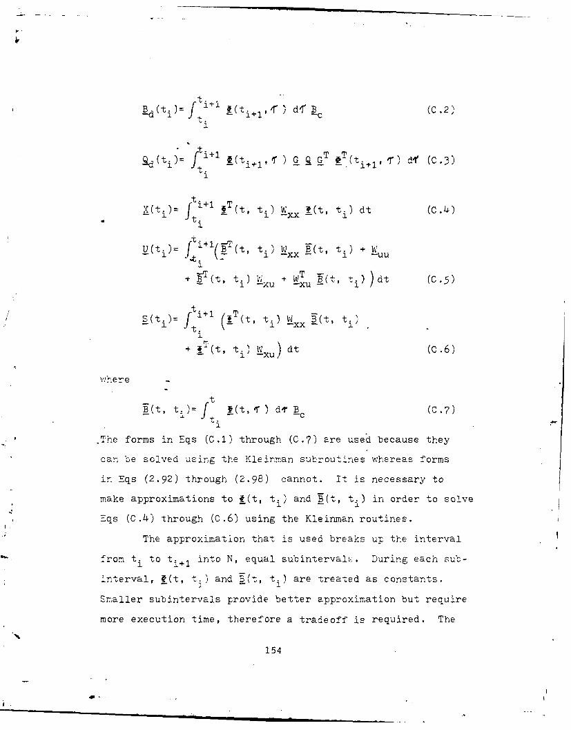
t. C (C .

(t)= 1 (t+ 1 G Q G (t) d (C.1)t. -

1

(t fti 1 §T(ti , ti V fGt d C4t. ~x - I+1 ) d c3

1[(i) l i + l _T(t, t i ) Wjxx T_(t, ti ) dt (C.4

+ T (t, t) v; + WT T(t, ) )dt (C.5)-uxu

t.1 T

+ _T(t, t i) W dt (C.6)1 XU)

where

tT (t, t i)= ft i (t, Ir ) dor B c(0.7)-- ti -c

The forms in Eqs (C.1) through (C.7) are used because they

can be solved using the Kleinman suhroutines whereas forms

in Eqs (2.92) through (2.98) cannot. It is necessary to

make approximations to ?(t, ti ) and B_(t, t i ) in order to solve

Eqs (C.4) through (C.6) using the Kleinman routines.

The approximation that is used breaks up the interval

tm t. to t. into N, equal subintervalc.. During each sub-

interval, 41(t, t,) and P(t, t,) are treated as constants.

Smaller subintervals provide better approximation but require

more execution time, therefore a tradeoff is required. The

154

" a.

subroutine that accomplishes the calculations of X(t ), S(t

and 1(t i ) allows the user to input the desired number of sut-

intervals, N. The routine then displays X(ti), U(t i ) and

(ti ) for that N, and allows the user to change the value of

and re c omnpu.te.

As stated above, constant values will be used over

%ach subinterval for (t, ti ) and !(t, ti. The constant

values used for the jth subinterval, fi and B. respectively,

are the average-values of I(t, ti ) and f(t, t i ) for the jth

subinterval. §(t, ti ) and B(t, ti) are calculated at the be-

ginning and end of the J th subinterval as well as a- three

equally spaced points between the beginning and the end.

These are the values that are averaged to form f. and B..

Thus, for At= (ti+ 1 - ti )

-average of t.) for all tE rt + (. - i-.j.veag -o z(t 1 i ,

t. + j tN_ .8

N

Baverage of "-(t, t9 for all te [t +(j-1 t

+ j At (C.9,

The Kleinman subroutine DSCRT simultaneously returns i(t, C'

and f E(t, ') d' and is the only major matrix subroutine0

needed in order to compute . and Bj,

Vhen the approximations just described for 0. and B.

are used, Eqs (C.4) through (C.6) become

155

• .

-- El I - - "

N

jx (t ) Z() N C.

-(tj= ! W-xx B- + -uu -+ T -xu - - (+ .1 )W B. B. 1

NNa(ti)= =~1( +., 41 j hX. A (C0.12)

Once values have been obtained for i(ti+1 , t ), B d(ti),

Qd(ti), X(ti), U(t i ) and S(t i ) it is still necessary to trans-

form Lqs (C.1) through (C.6) in order to use DRIC, the matrix

Riccati equation solver. The transformation of the LQ sampled-

data controller is (Refs 7 and 10)

Ei+l) 'ti+ , ti ) _t i ) + Bd(t i ) R_'(t i ) {.3

where

['t-~l t)= i(ti, t ) -Bt(ti) i s(ti) (C.14'

u'(ti)= u(ti) + U- (ti) S T(ti) x(ti) (C.15)

i-ow the quadratic cost equation that is minimized by

-'1 - *1+1) 4 L(tN+1 )

+ .fT ) ' x(t i ) + uT (ti) U(ti ) u ( i; (C.16)

- 11 - T_x t S I i)(C .1 -

:,'o," EoS (2.105) and (2.106) can be put into the format ofI

DRIC to solve for steady-state values of K' and G. In the

156

notation used in this thesis DRIC solves

K= IT 1 ( I + B U- 1 BT +) - 1 1 + K (C.18)-c - _ . . . - -

which can be obtained from Eqs (2.105) and (2.106) by setting

S(t.)= 0 and using the matrix inversion (Ref 8)

(I - YT(Z Y + W) -1 Z)=- (I + Y T w-1 0)- 1 (C.19)

and defining Y T= B, W= U, Z= BT Kc and I to be the identity

matrix. Note that (C.19) holds only when W (U in this case)

is positive definite.

Once G* is computed usinc the results from DRIC, C*_c

can be computed from

-2TG*= G*+ S (C.20)-c -C

Note, for W # 0 in the continuous-time case, the trans-

formation described in Eqs (C.13) through (C.17) and (C.20)

can be used if, in thoseequations, the Is are replaced by Fs,

Bds by Bs and Ss by W )s. Now Eqs (2.11) and (2.12) can be

used for the G* of the transformed system._c

As can be seen from the foregoing discussion, while

Kleinman's matrix software routines are very powerful, care

must be taken in order to arrange the equations properly so

that they match the arrangements used in these routines

(Ref 5).

157

Apendix D

Software Performance Verification

To verify the performance of the software developed

to support this thesis, several test cases with known results

were used.

For the continuous-time software, 3 test cases were

used. The first is example 14.25 in Maybeck (Ref 1). The

second is example 5.3 in Kwakernaak and Sivan (Ref 13). The

third is the example given by Doyle and Stein (Ref 2). The

details of these examples appear in Table D.I. In all cases,

the truth model and the controller design model are equival-

ent.

For the sampled-data software, the same three test

cases are used. The intent is to show that as the sample

period decreases, the steady-state value of P (t.) a---X t xt I

proaches the steady-state value of its continuous-time counter-

part, Pxtxt(t).

Table D.2 presents the results of the-software verifi-

cation run for both the continuous-time LQG regulator and the

discretized continuous-time LQG regulator. The results of

the continuous-time case are in agreement with the sources of

the examples (Refs 2 and 7). By examining Table D.2, it is

evident that as the sample period decreased, the performance

of the discretized controllers approached that of their con-

tinuous-time counterparts. Also note in the table that for

a sufficiently large sample period, the discretized control-

Clers do not approach the steady-state values of their contin-uous-time counterparts and may even diverge. This is ex-

158

reCied since the approxizrnaziorns used in discretization are not

valid for large sample periods.

Table the presents the results of the software verifi-

cation runs for the sampled-data LQG regulator software. As

in ihe discretized continuous-time case presented in Table

D.2, the performance of the sampled-data controllers approaches

that of their counterpart continuous-time controller for

sufficiently small sample periods.

159

TABLE D.1

Test Cases for Software Performance Verification

Test Case,1 (Ex 14.25 in Maybeck (Refl0) with T=2)

Program Inputs Expected Program, OutputsF= [-0.5] G= [1] Kf C.45=

B= [0.5 ] H= [1] 0 [O.5]

Q= [2] R= [3] mxt mu=[0]

PC=[ 1] x t = [0] [179]

Wuu0= [ 4] 0 Ext

Vjxu= o] - W =[ 5] Pu= [ 0.1045]

Test Case 2 (Example 5.3 in Kwakernaak (Ref 7))

Program Inputs Expected Program Outputs

F=- 1 001f=[40.361t0 -4.6 0 .1 1814.3]

0 i =[I 1 0] G*=[223.6 18.69]B= --

[0.781 _E=[ i0-7] Mxt= [ o T

Q= [10] o mu=[o]

[1 01 to [o, ooo4562 C]POP =

I':uu [0.00002] -xx 0 -u= [2.26]

xu: [0]

160

"q

TABLE D.i (con't)

Test Case 3 (Example in Doyle and Stein,' :'thout Robustness Recovery, (Ref 2))

Expected ProgramProgram Inputs Outputs

- Fo 1] B ] Kf[30 -50]-L1] G=[5o 10]

[ ,35] H[2 1] rn= [o oJG= ' -mt

L61 _ __ [i]Q= [i] -x [o o] _u [o]-- - Co [221 -613

F 0] -2800 473.3] x '

7,o 47 .3 80 L613 207:.: ':-uu= [1] -Alxu ' E o u=[ .(1o)4]

Test Case 4 (Same as Test Case 3 Except thatDoyle and Stein Technique is Applied)

Expected ProgramProgram Inputs Outputs

all program input matrices same asfor test case 3. Then when V= I and

a2= 100 '[26.8 -4o.2]-

236 -613]

Pxt 613 1810]

q2=50 50= [20.4 j 7.7] T

F 268 -613]

Ex - 6 1 3 150]

iooo: i [16.7 -1.9]-

F 285 -6131xt L-613 1360]

161

4-

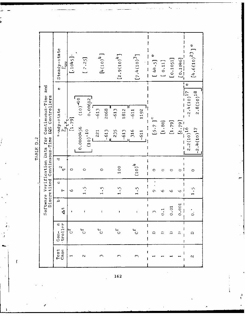
i j i01 1

4-' .

I' r0 * * - c

01 0

0 0, +j r-

Z 4-' co I- C

"0 . ~

< z 00-

- 4- Ci)

00 r- V 0 0J

*4- NN

0

L Q

4-'

4.-4

0

-P031

UWw

CC) C't' -4- -4 - N

162

C)~

C) 0 0

\ N0 0 0 0 0qV Cl \ l l CQ \, --M ~ ~ ~ ~ ~ --4 C -4' 0 \ \ 0 C 0 c \

N~ N N I C) I N

4LJ VL C C\J \ C'- \0 C~ C Cl 0 ' .

) N) 4 o~ N

I N

0 c0 0

c 0~

C) 0 '- I - I 1j0 E0 -0 .q

0 NO 0 0 ~ 163

C.) a)

-P ~4-' C) .

U) I 4- CC

00

_ 4'a)C C) a

C).' Cco X6

r4-1 4-1C

~ .~ 0

.- t 4--) -

I 4-' C) (

m' dC-4J 4-' 04-'~~~c CO C O .- )l- )C

-P~ ~~~~ if' ( N ) r~ ~i -O~~U Q) '- IU - t

N> 4 -4-

__ _ __ _ U) C) H 0

H 0 *- -H q 0- 4 Q

E-4~~E Nm- - 0 -0 0 C0

C) 4-H )

ofc - ~ C4-'. 4-1~

164 H

L ---

_ _ I

0- J ' y 0 00* 4 '- - 4\ N N I \ N N I N-

0 ) _4 ON N \C\I

qH a I >4 c 0 \ l

4- 0 0- d ICcI 4 0 l -4

C 0) N-- -- N~ "- C 1 . Cl \) C\ \-4

C\ \ * NI N \0

I Ct

4-110)

w~ N N

m _ __ _ __ __ __ __ __ __ __ _ __ __ __ __ __ __ ___165__ _

_ _

__________

C~7-1

U2~ 0

I L I N CQ -

C) *0 -4 N 1-4

co N

E--4r ir-1 11 r-

E-4 '4 I~I 4 I .

I 4-' ~0166

4-'4-'

0 4-' 4)

r~~ C) ~C)) 4'

oz 4' 4- -PC >

.a C).H 10C~2 Q C) ' 4o1 4-- Fz i to

4-D4-' H C) 0 C w 0

0' C) CH~ I4 ) 4C)

LO '- C C) 4- ) C3) 0-C) -44 -4-- c 4-)-P 4-D - - 0 0-- m) z~>od C) 4- 0~ 0 ) C

S CH *H Z: C -Cd U) --HU ) I' U

U) ri) 0f H ~ )0 U) a)~ H ~ 0C 4' C

H 0H 0' -1: - 4'C) ct C. ) -, Ci +D +D

::5 4- C) . ~4 4-> UC)0 0H 4 ~ C -

4S U)i a) U)r- ~ C-P c ~ l 0 V' C) U) E) 4Hz~-4 -P : 4- 0 ~ Lo 0 4-E-i~C 't Q)M -C) C) 0 ~ CH~

LO U) r l) ' Z 4-D 4 0U ) E) 4U)l, +

$z a) 4. $:: wC) C) b.0 .5- H

L-D -P4 5 - 0C C) 4-IC) U) a) 0) CC ) U) 'o C) 8 Q) Et o 0

H ) I~ W C) a)4-

4' b. C ) *H4-4- 4' 4 C) C) r- U)~ CE ) ' C) C) m 0 C) 0 - C) 0 V)c) C~ m~ mH -l1- 0 -C ' *1 U) 0 0.1 E- -H *H L) ' 0 C C

4' ) ' u 4'4 1 CH

cS Pfl -H C) c~ C) U+, C U) U)) 00 t3: C.o' 4-D C) >) *HL)H

r-I 4' '0 0) C)za-4- +- '4 >) > 'I O ~ 0 C ~ U

0 - 0 0-- *H *Ht 0)0 C) co z C)+)0 C

-~ ~ - J >167

;,pTendix EUsers Manual for

Linear Quadratic Gaussian Regulator Performance (IPQGRP

The purpose of this manual is to describe how to use

LQGRP to design and test linear Quadratic Gaussian Regulators.

The software provides the capability to enhance the robust-

ness of both continuous-time and sampled-data LQG regulators.4

The techniques used are described in a paper by J.C. Doyle

and Stein (Ref 2),inMaybeck section 14.5 (Ref 10),and in the

body of this thesis.

In-put

The program always begins in the input mod-. For the

first run through the program, a list of input/output options

(1-6) and a list of options to designate which vector/array

is to be input or output (1-21), is provided. These cptions

are presented in Table E.1. Note that when entering F or

R using options 11 and 13 respectively, the'value entered7 c

ma, be in either continuous-time or sampled-data format. User

response to prompts at other places in LQGRP is used to distin-

guish between the formats.

During the input mode of the program, the user selects

the desired vector/array to be input, then follows prompts

about entering I/o options, dimensions and vector/array ele-

merts. Note that option 18 allows all controller model mat-

rices to be equated to their truth model counterparts. The

number of deterministic states in the system models must also

be input at this time (see discussion under LQG Regulator

168

T illE -1

Input Routine Options

Matrix Vector Selection Cptions

Option £unction

i Truth model Ft matrix

2 Truth model Bt matrix

Truth model G t matrix

4 Truth model Ht matrix

5 Control.er design model F matrix6c

6 Controller design model B matrix-c m

Controller design model G matrix

9 Truth model initial covariance matrix, to

10 Truth model input noise strength matrix, Qt

11 Truth model measurement noise, strength matrix, Rt

12 Controller design model input noise strength matrix,Q c

13 Controller desigrn model measurement noise strengthmatrix, Ec

14 Truth model initial state vector, x

15 Control cost-weighting matrix, v'

-16 State cost-weighting matrix, 7' XX

, Cross (state-co-..trl,' cost-weighting matrix, C.-XU18 Equate F , O-c' f Q9 c to their truth model

countecr~artC

19 Terminate input mode, start regulator developmentmode

2C Store all matrices/vectors from options 1-17 tolocal file Tape?

21 Read all matrices/vectors 'or options 1-17 from

a fie T1re 6

169

L.

TABLE E.1 (con't)

Input/Output Options

IL

Option Action Taken

0 Terminate main program

1 Read entire array (row by row) or vector

2 Read entire array (row by row) or vectorand then print it

3 Read selected array or vector elements

4 Read selected array or vector elements

and then print them

5 Print the entire array or vector

6 or Return to calling program without taking.greater any action

170

Once a truth model and controller model have been com-

pletely entered and the cost-weighting matrices have been en-

tered, option 20 will store all this data to local file Tape7

for future use. Cnce a file Tare- has been created (and pos-

sibly stored as a permanent file) option 21 can be used to

read data from it if it is first copied into a local file

Tape8. Note any number of models can be entered during the

input mode and ztored to Tape7 for future reference.

Note any options 1-18, 20 and 21 can be executed any

number of times during the input mode. This allows for chang-

es to be made to specific vector/arrays in case an error iL

made. Option 19 terminates the input mode.

When the input mode is re-entered at the termination

of the performance analysis routine, any, all or none of the

options 1-18, 20, 21 may be executed.

Sto-p-ing LQGSIRP

LQ=z ma: ce aborted gracefully while in the input

mode. Simply choosing any option 1-17 and entering a zero

for the I/C option and (any number for the dimension required,

if required) will accomplish the abort.

Q. Regulator Set-Ur

Uoon leaving the input mode, the program enters the

,Qk regulator set-up mode. At this point the user must chccse

either a continuous-time controller or a sampled-data control-

ler. Note, there is provision in LQGRP to allow deterministic

171

(ie, states which are not controlled by input noise) states

(to be part of the system description. Note that such states

should be the first states in the state vector when entering

system model matrices in the input mode. The deterministic

states are removed from the system controller design model

before Kalman filter gain calculation. The Kalman filter gain

cbrresponding to those states deleted from the Kalman filter

gain calculations is set to zero.

Continuous-Time Controller

If the continuous-time controller is chosen, the user

has the option of calculating and displaying the eigenvalues

of both the truth model and controller model F matrices, of

modifying the G Q GT (used in the matrix Riccati equation for

calculating-the steady-state P matrix), and choosing the total

run time and the time increment between integration steps.

The modification to G Q GT referred to above was derived by

Doyle and Stein (Ref 1). Simply, it replaceg G Q G by Q(q)

where

Q(q)= G Q GT + q2 B V B

T

q 2is a scalar design parameter such that q-- causes the LQG

regulator to regain asymptotically the robustness character-

istics of a full-state optimal deterministic feedback LQ con-

troller. V is also a design parameter that must be Pny sym-

metric positive definite m x m matrix where m is the number

of inputs to the system input matrix B. Note, V= I is a good

first choice when there is no reason to weight the addition

172

of pseudo-noise to selected states. The filter poles, LQ

controller poles, and the LQG controller poles are computed if

the user wants to examine them.

Sampled-Data Controller

For sampled-data controllers, two basic options are

available. The first merely discretizes a continuous-timea

controller. The second developes a sampled-data controller

based on the matrices stored during the input mode.

In the first option, a continuous-time LQG regulator

is set-Up (see previous section) and is then discretized using

first order approximations. Note that when entering the time

increment for the continuous-time controller to be discretized,

the time increment will become the sample-period of the discrete-

time controller.

In the second option, an appropriate sampled-data con-

troller is set up using the values entered during the input mode.

In this option an approximation to the values of the continuous-

time cost-weiahting matrices, X(ti), U(ti) ad S(ti) for

sampled-data controllers is made. A discussion of this

approximation is in Appendix C. Briefly, it entails using

constant values for certain matrices for each of a number

of subintervals of the sample-period. The more subintervals,

the better the anproximations, but the more computer time

required.

Also in the second option, there are two design options

for increasing robustness properties of the controller. The

first is a discretized version of the Doyle and Stein technique

173

described previously in the continuous-time section. The

second option for increasing robustness involves picking K,

(the Kalman filter gain directly such that

2= g B W

where I is the controller design model state transition matrix,

!d is the discrete-time input matrix and W is any nonsingular

m x m matrix where m is the number of inputs to the system. The

user has the option of picking any W or of calculating

W= (H I- I B d)- as in Maybeck (Ref 10). As in the continuous-

time case, q is a scalar design parameter that, as q--, asympto-

tically causes the LQG regulator to recover the robustness

characteristics of the full-state feedback optimal deterministic

LQ regulator. As in the continuous time case the filter poles,

LQ controller poles and the LQG regulator poles are computed if

the user wants to examine them.

Performance Analysis

After the LQG regulators are properly.formatted by the

aforementioned routines, a covariance analysis is performed.

This analysis is described in the body of the thesis. First a

set of augmented system matrices are formed and then the

performance analysis begins. Eqs (E.1) through (E.8) describe

the augmented system used in the performance analysis.

xT= xT xT (Ei)-za= fa-a + B Yd + a a t

where

tft -t -cz -t -t PcxFa B f(E.2)

174

Bt c Y(E.52 _[ao .i 'cz (E-'

w_ (E6ixtJ

and then

MXa(t)= -fl(t' to ) Mxa(to)xa , mxa

Note fn(1 tho) ( ) ior smd-dta stm

Ex Xa a th auxe~e : 7 :;a I Z

t

- 0

Tha t , ot o n - ao tprinting out the augmented

system matrices. The user also has the option of sy-ecifying

hoemany time increments there should be between plot points

and points printed at he terminal for Pxa and F :he Co-

variance of the augmented system and the controller, respec-

~tively.

175((

wm w I

Te plot points are formatted and stored to a series

of local files as follows:

m -a Tape 12Mxt

Fx - Tape 13

Mu - Tape 14

Puu - Tape 15

where mx t is the mean of the truth model states, Pxtxt is the

covariance of the truth model state ( only diagonal entries

are written to Tape 13), mu is the mean of the controls gen-

erated and P u is the covariance of the conttols generated

(only diagonal entries are written to Tape 15).

Each performance analysis run is tagged with a run

number, total time, sample-time and the dimension of the state

vector or control vector as appropriate. This is the first

record of information written to the local files, Tape 12

Tape 15 for each run. The last two records written to these

files for each run contain the minimum value of the data array

and a scale factor; both are needed for plotting.

Upon exit from the performance analysis routine, the

program re-enters the input mode and changes the run number.

Plotting

In order to plot the data, it is necessary to abort

the LQGRP program and execute the plotting program, MYPLOT

on a terminal connected to an HP plotter. If the HP plotter

176

is unavailable or unacceptable for some reason, MYCLPT will

generate a Calcomp plot file at a terminal that can be routed

to the Calcomp plotter.

Either MYPLOT or MYCLPT reads data-formatted by the

performance analysis routine off any local file, Tape xx

(where xx is 12, 13, 14, or 15). Note that if the user wishes

tGo do any manipulation of the data tapes before using this

program, the result can be stored on any tape numbered 1

through 99. This number can be used in place of 12-15 as

indicated earlier. Before plotting it gives the user the

option to preview the data. Note, when previewing, the user

should check to be sure the last two data entries are the

minimum value and the scale factor, respectively.

After each plot, the user has the option to abort,

plot a different variable (ie, xt instead of xtl), read andt2 t1

plot the next run of data from the same tape, or read and

plot data from a new tape. All options executed in either

program are results of user inputs to self-explanatory program

prompts printed at the terminal.

177

4'!

I.|m

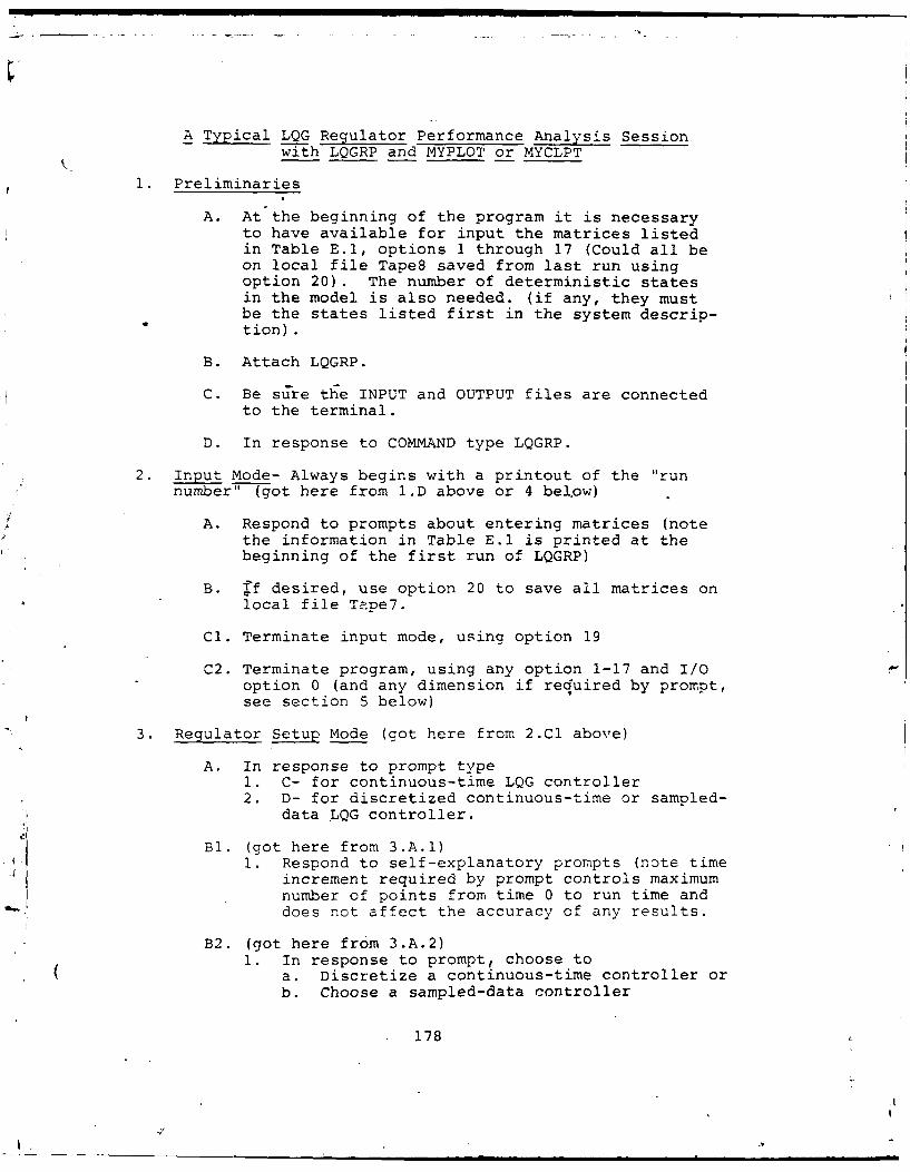
Typical LQG Regulator Performance Analysis Sessionwith LQGRP and MYPLOT or MYCLPT

1. Preliminaries

A. At the beginning of the program it is necessaryto have available for input the matrices listedin Table E.1, options 1 through 17 (Could all beon local file Tape8 saved from last run usingoption 20). The number of deterministic statesin the model is also needed. (if any, they mustbe the states listed first in the system descrip-tion).

B. Attach LQGRP.

C. Be sure the INPUT and OUTPUT files are connectedto the terminal.

D. In response to COMMAND type LQGRP.

2. Input Mode- Always begins with a printout of the "runnumber" (got here from I.D above or 4 bel.ow)

A. Respond to prompts about entering matrices (notethe information in Table E.1 is printed at thebeginning of the first run of LQGRP)

B. ff desired, use option 20 to save all matrices on

local file Tape7.

Cl. Terminate input mode, using option 19

C2. Terminate program, using any option 1-17 and I/Ooption 0 (and any dimension if required by prompt,see section 5 below)

3. Regulator Setup Mode (got here from 2.Cl above)

A. In response to prompt type1. C- for continuous-time LQG controller2. D- for discretized continuous-time or sampled-

data LQG controller.

Bl. (got here from 3.A.1)1. Respond to self-explanatory prompts (note time

increment required by prompt controls maximumnumber of points from time 0 to run time anddoes not affect the accuracy of any results.

B2. (got here from 3.A.2)1. In response to prompt, choose to

a. Discretize a continuous-time controller orb. Choose a sampled-data controller

178

2a. (got here from 3.B2.1.a)1. Note that when entering time increment for

continuous-time controller it will becomethe sample-time of the discretized con-troller and affect stability.

2. Follow the remaining prompts.2b. (got here from 3.B2.1.b)

1. Answer prompts2. In response to prompt about subinterval

for calculating X, S and U, remember abetter approximation is obtained for moresubintervals but that this requires more

b computer time.3. Follow remaining self-explanatory prompts.

4. Performance Analysis Mode (got here from 3.B1 or 3.B2)

A. Be careful in selecting number of prints at termi-nal (in response to prompts) of m , mu, P andP since the printouts require a C_Al aUsignificant amount of time and paper.

B. Be careful in choosing the number of points to goon the plot files (in response to'prompt) sincethe number of points significantly affects plot-ting times. (For example,-100 points plotted onthe HP plotter takes about 5 minutes, 200 pointsapproximately 10 minutes etc..... .:ith 200 pointsto be plotted, there will be more than 20 points-lotted per inch since the time axis of the plotis scaled to 7 inches).

5. Data File Plotting/Storing (got here from 2.C2)

A. If data was saved on Tape7 using option 20, nowis the time to create a nermanent-file of thisdata (see terminal operations manuals,

B. if you don't have time to plot the data on localfiles Tapel2, Tapel3, Tapel4 and Tape 15, now isthe time to create permanent files for this data.

B2. 1.ant to plot data from todays run or from previousruns stored on permanent file.1. Make sure files are rewound before use2. Atch cory. of TVYPLO or ,.YCLPT depending on

where you want the 'clots made.a. Type MYPLOT or ,YCLPT in response to "COM-

MAN *'.,

b. F oio.' prompts C-e. -CaZ I .: ct r atAFIT can only handle 5 plots per plot file.It is necessary to terminate MYCLPT (fol-lowing self-explanatory prompts) aftereach set of 5 plots is created. Then theplot file should be routed to the plotter,

179

and then MYCIPT can be re-entered for the

ncex 5 plots).

C. If you are using MYC?' , the plot fLe

.uat be routed to the plotter at the termDi-

nation of KYCLPT.

180

ArpendiX F

Anollo Model Performance Data

This appendix contains additional mean and covariance

plots used to support the results and conQlusion of Chapter

181

AD A115 478 AIR FORCE INST OF TECH WRIGHT-PATTERSON AF8 OH SCHOO--ETC FIG 1/3ROBUST CONTROL SYSTEMS.IU)DEC 81 ED0 LLOYD

UNCLASSIFIED AFIT/GE/EE/SI0-36 NL

INhhhhmh7h82

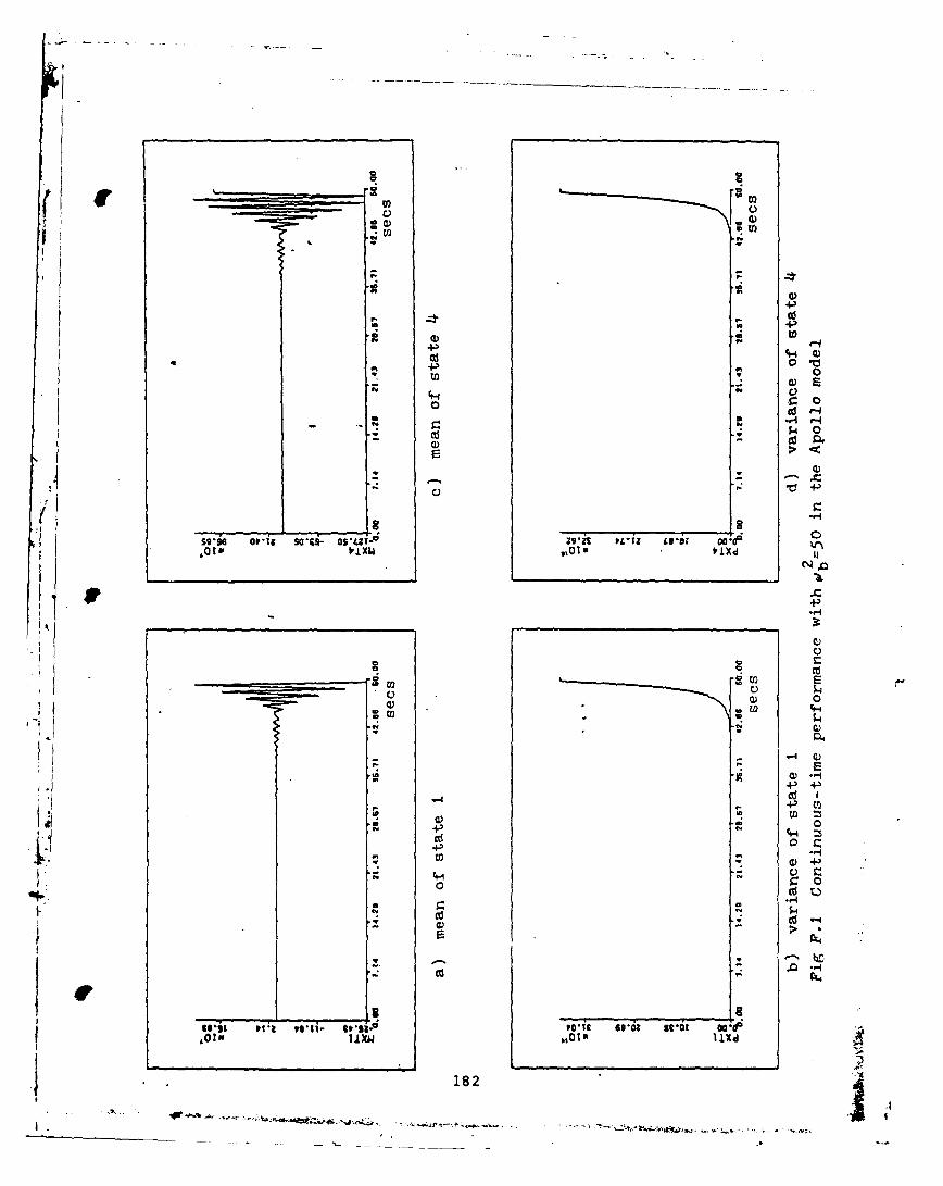
(VO

UC

$ CIS

Q) 0

04-4-

C* C W 4

1822

C D

0 E

ed0

a) W

it. a -0 0

-4-'

0) 4-

ccd

zz

aO~ soa t00t;ax

183

Wvow

C.) U

Lo

0

0 r.

d0

0e oz a auo6- 60*-0 a Wo 43

C

-to-cV 4-

a) C)C) C)

ww

. C.

9010 30. 106- LO-0-0 $0. to a 30. 04d

4 - .184

CD CD

*0d

w~

V

C.

CdC

r= >

CD I

46 0

cotQ)4

e.

I Li

185 I

0V3(I))

Cd)

00

wo s ) o*- 0 - 1400: lzo c

A C14

p4

a) CL

0

* C

a8186

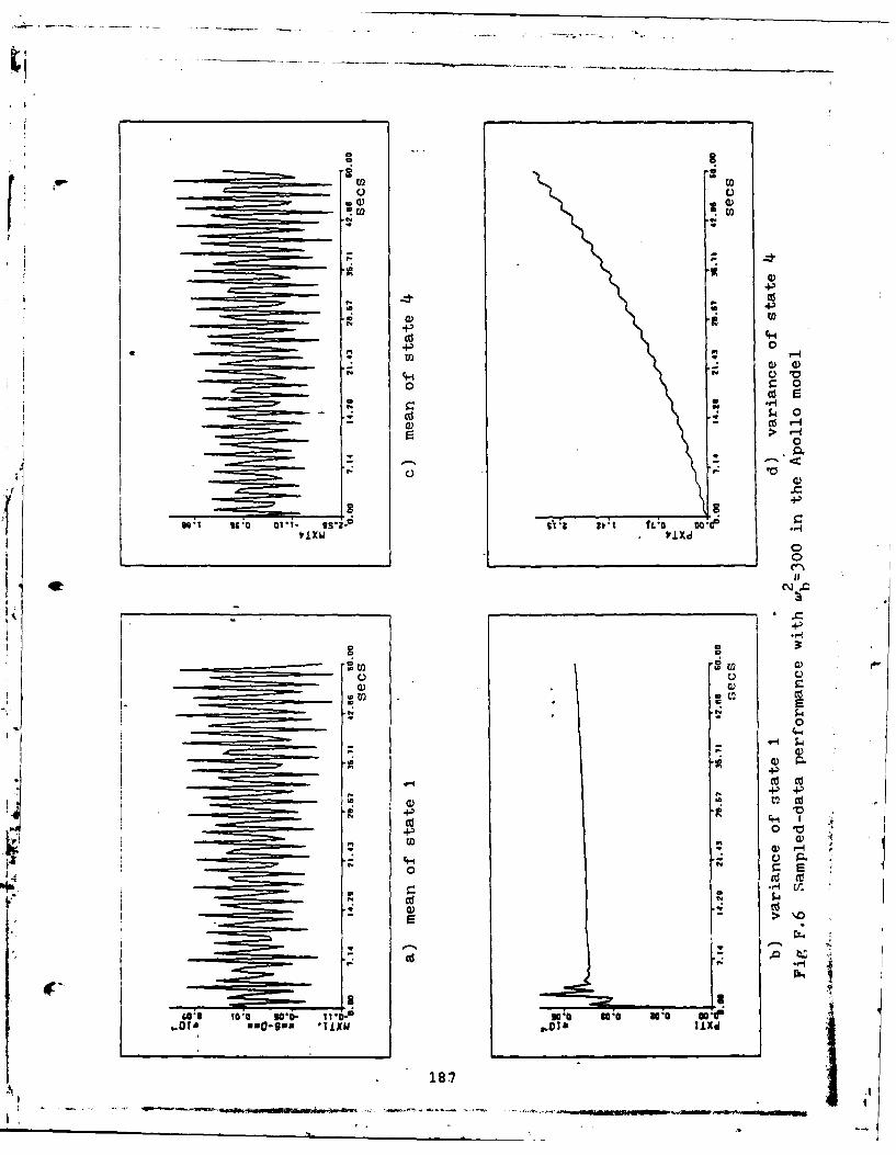
od 0

WV U. aai siPo d0

40 U~

tv C

00

7 u

m C) E00

Ed )c

8 _ _ _ _ _ _ _ _ _ri

a.l 00 -2 la ~i

0180

CD a)

0 .r. .14co S

0 90

EE

Sd C

CdC__ _ _ __ _ _ __ _ _ __ _ _ 0

to,

o o f*a s W0Ia o* 0I SWli~

18

(1) w

4

- I.

to to

0) 0

4-1

CD Cd

0

to w Q)

Cd S-i

0)0

Cdt 0

-P

0)

4-4 u

co CH V2

C ad

C1L4

0p ~ 016 0r G 9. o0 W

too, 189

0 aa

Ina

(7W

4-4-

00

C.)

10 m

to C)

0

> N

so 0 10a 1-- 9 a o 0 t 0 3 o

,.DID ~~ Ix DNIx

19- - - - - - - - - - - - - - - - -

Id0 j' 0

o 0

.0 C0

4.)P4

0- 00

a 2T-6 woP0. O- 9--

191

viTA

Eric Dean lloyd was born on 26 August 1951 in Key West

Florida. He graduated from high school in Glendale, Arizona

in 1969 and then attended Glendale Community College. In

June 1970 he enlisted in the USAF and was trained as a com-

puter repair specialist. In 1971 he applied for and was ac-

cepted in the Airman Education and Commissioning Program.

Through this program he earned the degree of Bachelor of

Science in Electrical Engineering from the University of

I issouri - Columbia, Missouri, in 1974. After his commis-

sioning through the Officers Training School he was assigned

as an instrumentation engineer and ground systems test'con-

troller for the Minuteman III Weapon System Research and

Development testing at Vandenberg AFB, California. Follow-

ing that, ht was assigned in a two year Space Shuttle Test

Director training program with the National Aeronautics and

Smace Administration at the Kennedy Space Center, Florida,

until entering the School of Engineering, Air Force Institute

of Technology, in June 198C.

192

UNCLASSIFIEDSECURITY CLASSIFICATION OF THIS PAGE (When Dfltb nftered)

REPORT DOCUMENTATION PAGE RE:AD iNSTRUCTIONSRP TDO tEFORE COMPLETING FORM

I. REPORT NUMBER J2. GOVT ACCESSION NO. 3 RECIPIENT'S CATALOG NUMBER

( -AFIT/GE/EE/81D-36 4b- *171 54 TITLE (and Subtitle) J0 5 TYPE OF REPORT & PERIOD COVERED

C NS THESISROBUST CONTROL SYSTEMS 6. PERFORMING 01G. REPORT NUMBER

7 AUTHOR(s) 8. CONTRACT OR GRANT NUMBER(S)

Eric D. Lloyd

Capt USAF9 PERFORMING ORGANIZATION NAME AND ADDRESS 10 PROGRAM ELEMENT. PROJECT. TASKAREA & WORK( UNIT NUMBERS

Air Force Institute of Technology(AFIT/EN)Wright-Patterson AFB, Ohio 45433

II. CONTROLLING OFFICE NAME AND ADDRESS 12 REPORT DATE

DEC 198113. NUMBER OF PAGES

202

14. MONITORING AGENCY NAME & ADDRESS(f different from Controlling Office) IS. SECURITY CLASS. (of thte report)

ISa. DECLASSIFICATION DOWNGRADING'ffH E -.U L

E ..

ca sfiled16. DISTRIBUTION STATEMENT (of this Report)

CApproved for public release; distribution unlimited.

II, DISTRIBUTION STATEMENT (of the abstract entered in Block 20, If different from Report)Dean for Research and

1 5 APR 1882 Professional Develomn-tAir Force Institute of Technology (ATC)

;1) Wright-PattersonAFB.H 454131. SUPPLEMENTARY NOTES

Approved for release; IAW AFR 190-17

FREEtI C . YNMao-JS) F

Directrf A c irsIS. KEY WORDS (Continue on reverse side It necesseary and Identify by block number)

Robust Control Systems, LQG Controllers, Kalman Filters,Optimal Stochastic Controllers

20. A6s TR CT (Continue on reveres side If neceseary and identify by block number)

The Doyle and Stein robustness enhancement techniquefor continuous-time LQG stochastic controllers was investigatedin application to simple examples and a realistic ApolloCommand Service Module/Lunar Module Thrust Vector ControlSystem that exhibited severe robustness problems in its initialdesign. This technique was then extended to discrete-time

DD I FN 1473 EDITION OF I NOV 65 IS OBSOLETE UNCLASSIFIEDSECURITY CLASSIFICATION OF THIS PAGE (W% n Data Entered)

.. .. .. .. ----- .

I i NrT.ARSIFIED-Sz'% ITY CLASSIFICATION Of THIS PAGE(MVho Date Znjoed

systems in two ways. First, the continuous-time controller

to which the Doyle and Stein technique had been applied wasdiscretized using first order approximations. Second, an

approximation to their continuous-time technique was developedfor sampled-data control systems. In addition, an attemptwas made to enhance the robustness of sampled-data systemsby directly picking the gain of the Kalman filter within thecontroller structure based on an approach similar to thatof Doyle and Stein.

Sampled-data ctr-ollers were designed using each of theseapproaches. The resulting performance analysis for eachclosed-loop system was based on the time histories of themean and covariance of the "truth model" states and controlsas well as on the eigenvalues of the closed-loop system. Inboth the discretized continuous-time and sampled-data cases,significant steady-state robustness enhancement was observed.Results for picking the Kalman filter gain directly wereinconclusive. General purpose interactive software fordeveloping robustified LQG controllers was also produced anddocumented.

UNCLASSIFIED

SFCIIRITY CLASSIFICATION OF -AG W'.. 1.* W..

41)DAT

FILM

VDT