Air Monitoring Guidelines for Petroleum

Refineries

AIR DISTRICT REGULATION 12, RULE 15:

PETROLEUM REFINING EMISSIONS

TRACKING

Prepared by the staff of the

Bay Area Air Quality Management District

August 2015

i | P a g e

DRAFT: 8/10/15

Air Monitoring Guidelines for Petroleum Refineries

Table of Contents

Executive Summary ........................................................................................................................ 1

Background ..................................................................................................................................... 2

Section 1: Basic Requirements for an Approvable Air Monitoring Plan ..................................... 5

1.1 Fence-line Monitoring ................................................................................................. 5

1.2 Community Monitoring ............................................................................................... 6

1.3 Display of Monitoring Information ............................................................................. 7

Section 2: Air Monitoring Guidance Document and Development of Air Monitoring Plans ....... 8

2.1 Components of Monitoring Near Refineries ............................................................... 8

2.2 Data Display and Dissemination ................................................................................. 9

Section 3: Considerations for Fence-line Monitoring .................................................................... 9

3.1 Open Path Monitoring ............................................................................................... 10

3.2 Appropriate Sampling Locations ............................................................................... 12

3.3 Appropriate Sampling Methodologies ...................................................................... 12

3.4 Quality Assurance/Quality Control (QA/QC) ........................................................... 12

Section 4: Monitoring Based in the Communities around Refineries ........................................ 13

4.1 Likely Risk Drivers and Near-field Gradients .......................................................... 14

4.2 Fixed Community Monitoring ................................................................................... 15

4.3 Appropriate Sampling Locations ............................................................................... 16

4.4 Appropriate Sampling Methodologies ...................................................................... 17

4.5 Quality Assurance/Quality Control (QA/QC) ........................................................... 17

Section 5: Data Display/Reporting ............................................................................................. 17

5.1 Time Resolution and Data Availability ..................................................................... 18

Section 6: Siting Considerations ................................................................................................ 19

6.1 Nearby Structures ...................................................................................................... 20

6.2 Terrain ...................................................................................................................... 20

ii | P a g e

6.3 Meteorology ............................................................................................................. 20

Section 7: Multi-pollutant Monitoring .......................................................................................... 20

7.1 Black Carbon ............................................................................................................. 21

7.2 H2S* ........................................................................................................................... 21

7.3 NO2 (Nitrogen Oxides)* ............................................................................................ 21

7.4 Particulate Matter (PM) ............................................................................................. 21

7.5 PM constituents ......................................................................................................... 22

7.5.1 Elemental Carbon/Organic Carbon (EC/OC) ............................................................ 22

7.5.2 Metals ........................................................................................................................ 23

7.5.3 PM number concentration ......................................................................................... 23

7.5 Speciated Hydrocarbons* .......................................................................................... 23

7.5.1 Aldehydes* ................................................................................................................ 24

7.5.2 Polycyclic Aromatic Hydrocarbons (PAH)* ............................................................. 24

7.5.3 Volatile organic compounds (VOCs)* ...................................................................... 24

7.6 SO2* ........................................................................................................................... 24

7.7 Surrogate Measurements* ......................................................................................... 25

Appendix 1: DRI Report ...................................................................................................................

Appendix 2: Expert Panel Report .....................................................................................................

1 | P a g e

Executive Summary

On August 6, 2012, a substantial fire occurred due to a hydrocarbon leak at a crude oil

processing unit at the Chevron Refinery in Richmond, California. The fire resulted in a large

plume of black smoke and visible emissions from a refinery flare. The August 6, 2012 incident

prompted the Bay Area Air Quality Management District (Air District) staff and Board of

Directors to identify a series of follow-up actions to enhance the Air District’s response to

similar incidents (Board of Directors, October 17, 2012). One of these actions was to convene a

panel of air monitoring experts (Expert Panel) to recommend technologies, methodologies and

tools to enhance community air monitoring capabilities near refineries. In order for the Expert

Panel to have a uniform starting point for their discussion, the Air District contracted with

Desert Research Institute (DRI) to compile a report that provided background on current air

monitoring capabilities near refineries and potential air monitoring technologies,

methodologies and tools that could be used at refinery fence-lines and in the community to

determine impacts from normal refinery operations and episodic incident-based releases.

Another related follow-up action was the development of a new Air District Petroleum Refining

Emissions Tracking rule, which would include a requirement that Bay Area refineries establish

and operate fence-line and community air monitoring systems consistent with guidelines to be

developed by the Air District.

The purpose of this Guidance for Air Monitoring Near Bay Area Refineries is to provide a

framework on how these air monitoring systems should be developed and deployed and what

metrics the Air District will use to evaluate the ability of those systems to meet the goals

outlined below. The Guidance provides refineries with information to be used to develop an air

monitoring plan that the Air District will review, provide feedback and/or recommendations

and approve once the monitoring plan meets the goals of the monitoring effort.

2 | P a g e

Background

On August 6, 2012, a substantial fire occurred due to a hydrocarbon leak at a crude oil processing unit at the Chevron Refinery in Richmond, California. The fire resulted in a large plume of black smoke and visible emissions from a refinery flare. The Contra Costa County Health Department issued a community warning and ordered a shelter-in-place for approximately five hours in Richmond and San Pablo. Thousands of residents sought medical treatment, with most suffering respiratory and/or eye discomfort.

The August 6, 2012 incident prompted the Bay Area Air Quality Management District (Air District) staff and Board of Directors to identify a series of follow-up actions to enhance the Air District’s response to similar incidents (Board of Directors, October 17, 2012). One of these actions was to convene a panel of air monitoring experts (Expert Panel) to recommend technologies, methodologies and tools to enhance community air monitoring capabilities near refineries. Another related follow-up action was to expedite the development of a new Air District Petroleum Refining Emissions Tracking rule, and to include a requirement that Bay Area refineries establish and operate fence-line and community air monitoring systems consistent with guidelines to be developed by the Air District. This guidance document is intended to provide a framework on how these air monitoring systems would be developed and deployed and what metrics the Air District will use to evaluate the ability of those systems to meet the goals outlined below.

As part of the effort to develop this guidance, the Air District contracted with Desert Research Institute (DRI) to compile a report that provides background on current air monitoring capabilities near refineries and potential air monitoring technologies, methodologies and tools to:

Provide air quality information for communities near refineries

Gather data to evaluate health impacts associated with air quality near refineries

Track air quality changes and trends over time near refineries

The DRI report reviewed and evaluated measurement approaches and methods for assessing the impacts of refinery emissions on ambient concentrations of criteria and air toxics pollutants in nearby communities and is included in Appendix A. Available data for refinery emissions along with ambient air concentrations were reviewed and compared to established levels for acute and chronic health effects to identify the species that should be considered for air monitoring. Various monitoring options were associated with the following monitoring objectives: short-term characterization of emission fluxes; long-term continuous fence-line monitoring of refinery emission releases to the community; community-scale monitoring with varying time scales to evaluate potential chronic or acute health impacts; and episodic monitoring during catastrophic events. With these objectives in mind, air quality data from existing Air District criteria and air toxics pollutant monitoring programs, and air monitoring (both regulatory and voluntary) by the refineries were then used to identify existing gaps in information or useful supplemental data. Published results from relevant applications of the

3 | P a g e

monitoring approaches were reviewed and the specifications for selectivity, sensitivity, precision, accuracy and costs of commercially-available continuous or semi-continuous monitors, and time-integrated sampling and analysis methods were compared for each target pollutant to determine the positive and negative attributes of each monitoring approach and method. Potential augmentations to existing monitoring in the Bay Area were suggested with scalable options. It was the intent of the Air District to utilize the DRI report to provide the Expert Panel with a starting point for further discussion.

The Expert Panel was convened on July 11, 2013 and included monitoring experts from around the nation representing academia, community advocates, industry and government. The final report of the Expert Panel, including a list of participants is provided in Appendix B. The Expert Panel reviewed the DRI report, received a presentation by one of its authors, Mr. David Campbell, and then addressed questions developed by the Air District to further explore potential air monitoring methodologies and instrumentation that could be developed to provide the public, refineries and regulators information about exposures to the public near refineries. The questions that the Expert Panel addressed were:

What should the size and spatial orientation of a network of monitors be around refineries?

What network components should be considered (compounds measured, technology and instrumentation used, methodologies applied, air quality assessment tools utilized, etc.)?

How should the data be provided to the public?

What should be considered when developing measurement quality objectives, such as: o What type of instrument siting criteria should be used? o What should the time resolution of the equipment be? o How often should the instrumentation be calibrated? o What should the accuracy/precision/completeness requirements of the data be? o What other quality control/quality assurance requirements should be put in

place?

What technologies, methodologies and tools could be employed to augment any fixed network to better quantify pollutant variations over space and time, especially during short duration incidents?

What emerging technologies might be utilized in the future to further enhance community air monitoring capabilities?

The Expert Panel believed that open path monitoring capable of measuring representative compounds at near-ambient background levels of detection likely to be emitted by refineries should be employed at, or near, refinery fence-lines. Measurements of these compounds should be collected at a time resolution of 5 minutes. Data should be displayed to the public real-time, with appropriate QA/QC parameters defined and context provided so that the public can more easily understand when concentration from refineries reach levels of concern.

4 | P a g e

The Expert Panel believed that defining chemical composition and concentration gradients as distance away from refinery fence-lines increased was critical and that monitoring within the community be tied to these gradients. The DRI report and the Expert Panel acknowledged that there were available methods that could be utilized to represent gradients, such as flux measurements and modeling, around refinery property. For purposes of this Guidance Document, the term “gradient” will be used to represent any of these techniques that can adequately represent gradients as distance increases from the fence-line into the community. The Expert Panel also believed that no more than three community monitoring locations were necessary. They believed that compounds associated with risk and measured at other air monitoring locations should be included in the community monitoring locations, even if those compounds were not emitted by the refinery, so that the community could compare concentrations and associated risk to other locations.

The Air District has developed this Guidance Document for monitoring near refineries based on the DRI report and the input provided by the Expert Panel. This Guidance Document can be used by the refineries to develop Air Monitoring Plans as described in Air District Regulation 12, Rule 15. The guidance is intended to identify what should be included in the Air Monitoring Plan and what must be provided to the Air District in order to deviate from specific recommendations and satisfy flexible conditions of the guidelines. The Air District recognizes that, in certain circumstance, flexibility must be provided in order to allow for operational or technical limitations of instrumentation or sampling methodologies and has identified where that flexibility may be used as long as acceptable rationale is provided that outlines the operational or technical limitations. In addition, the Air District will use this Guidance Document as a basis to evaluate whether Air Monitoring Plans and the monitoring systems contained therein adequately address the monitoring goals of measuring compounds of interest near refineries and reporting them to the public. The Air District encourages the inclusion of the community and other interested parties in the development of Air Monitoring Plans to help ensure that the community’s concerns and desires are adequately addressed. Revisions and updates to this guidance will be required as new instrumentation, methodologies and monitoring strategies are developed. Staff will bring any substantial changes to the Board of Directors for their consideration of approval.

5 | P a g e

Section 1: Basic Requirements for an Approvable Air Monitoring Plan

This Section describes the criteria for an approvable Air Monitoring Plan. Plans that meet these criteria will be considered by the Air District and approved if all criteria in this Section are met. However, as part of the approval process, the Air District will consider comments received during the public comment period. This Guidance Document provides additional information in later sections that demonstrates pathways to alternatives and outlines processes and considerations for meeting the requirements of developing an Air Monitoring Plan. Where air monitoring requirements described in this Section are not met, subsequent Sections outline what a refinery owner/operator should provide as a rationale for why the Air Monitoring Plan should be approved. Such rationale will be evaluated on a case-by-case basis.

1.1 Fence-line Monitoring

Refinery operators must measure benzene, toluene, ethyl benzene, and xylenes (BTEX) and H2S concentrations at refinery fence-lines with open path technology capable of measuring in the parts per billion range regardless of path length. Open path measurement of SO2, alkanes or other organic compound indicators, 1, 3-butadiene, and ammonia concentrations are to be considered in the Air Monitoring Plan. Refinery operators must provide a rationale in the Air Monitoring Plan for not measuring all of the above compounds that addresses: why these compounds are not contained in the compositional matrix of emissions; are not at expected concentrations measured by available equipment; and/or, address the technical or other considerations that make specific measurements inappropriate or unavailable. Fence-line measurements must be continuously measured with a time resolution of five minutes. If this is not the case, refinery operators must provide rationale in the Air Monitoring Plan for lesser time resolutions based on equipment or other operational limitations. These measurements must be provided to the public on a real-time basis, with appropriate Quality Assurance/Quality Control (QA/QC) measures taken to provide assurance of data accuracy. A Quality Assurance Project Plan (QAPP) that follows EPA guidelines must be developed that outlines the QA/QC parameters. Instrumentation must meet a minimum of 75% completeness on an hourly basis, 90% of the time based on annual quarters. Atmospheric conditions beyond the control of the refinery that affects accurate measurements, such as dense fog, shall not be counted against data completeness requirements as long as appropriate meteorological measurements document time periods when these conditions exist. Measurements must cover populated areas within 1 mile of the refinery fence-line likely to be affected when the annual mean wind direction lies in an arc within 22.5 degrees of a direct line from source to receptors 10% of the time, or greater, based on the most representative meteorological measurements for sources likely to emit the compounds listed above at the refinery. If this is not the case and an alternative method, such as dispersion modeling is used to determine fence-line locations, refinery operators must provide rationale for utilizing any

6 | P a g e

alternative in the Air Monitoring Plan that addresses why receptors would not be affected by emissions from the sources within the refinery. Refineries that already have open path monitoring capabilities in place need only provide verification those current systems adequately address population requirements. 1.2 Community Monitoring

Refinery operators must appropriately site and operate at least one permanent community air monitoring station that provides a reference for exposures for residents living near the refinery. Concentration gradients from the refinery fence-line will be used by the refinery to develop correlations to the compounds (see below) measured within the community to determine where and how many stations must be installed. Other measurement techniques may be used to determine gradients, such as component flux across the fence-line, or appropriate modeling techniques. The methodology chosen for determining gradients, and the rationale for this choice, must be provided and approvable in the Air Monitoring Plan. The term “gradient” will be used throughout this Guidance Document to represent the approved methodology. The Air Monitoring Plan must outline how permanent site(s) will be chosen and correlations and relationships with gradients established. In addition, methodologies must be provided to determine how often gradient measurement must be repeated to demonstrate that correlations and relationships continue to be valid. Gradient measurements, or appropriate alternatives, must be repeated every seven years, at a minimum, or when equipment or processes change significantly. The Air Monitoring Plan must provide rationale for when gradient measurements or appropriate alternatives will be repeated. Multiple stations must be considered where chemical component mixtures differ in composition and/or differ in concentration by such that overall risk, as defined by Health Risk Assessments required as part of Regulation 12, Rule 15, is greater than 10 in one million. Rationale supporting the number and location(s) of community monitoring stations as well as the methodology for determining correlations to gradients, must be supported and approvable in the Air Monitoring Plan. Measurements of a surrogate for diesel particulate matter (DPM), such as black carbon, total hydrocarbon, or other representative hydrocarbon measurement, speciated hydrocarbons based on TO-15 including BTEX, 1, 3 butadiene and carbon tetrachloride, oxides of nitrogen, SO2 and particulate matter less than 2.5 microns in diameter (PM2.5) shall be measured at community monitors. Filter-based measurements that can be analyzed for metals, semi-volatiles, and other PM species must also be considered in the Air Monitoring Plan. If the above compounds are not included, refinery operators must provide a rationale for not measuring the above compounds that addresses: why these compounds may not be contained in the compositional matrix of ambient air; and/or, are not at concentrations measured by the equipment and analytical techniques available. In addition, if multiple community monitoring

7 | P a g e

locations are indicated and not proposed, refinery operators must explain how developed correlations will adequately represent the number of locations proposed. Community monitoring locations must continuously measure total hydrocarbons, or other representative hydrocarbon measurement, and oxides of nitrogen and provide at least hourly measurement of PM2.5 using a federal reference or equivalent method. Black carbon must be measured on at least an hourly averaged basis unless a filter based Elemental Carbon/Organic Carbon (EC/OC) method is used. Samples collected for TO-15 analysis and filter based sampling must be conducted every twelve days, at a minimum, and must be a twenty-four hour integrated sample. Federal and/or State sample collection and analytical methods must be used, where available. If Federal and/or State methods are not available, best industry practice must be utilized and rationale as to why a method is an “industry best practice’ provided as part of the Air Monitoring Plan. Results must be provided to the public on a real-time basis, where possible, and when results become available for parameters that require laboratory or other analysis to provide results. All QA/QC techniques must be outlined in a QAPP that follows EPA guidelines. Data completeness must be maintained at 80% for all compounds with continuous measurements meeting 75% completeness on an hourly basis 80% of the time based on annual quarters. Measurements must be taken in a location that is representative of the population living near the refinery and be correlated to gradients caused by emissions from the refinery as described in this document. The siting of this location must meet the requirements of 40 CFR Part 58, or the refinery operator must provide rationale on why there should be allowable deviations from these requirements, explaining how those deviations do not bias measurements to be lower than expected. 1.3 Display of Monitoring Information

The data must be displayed to the public as defined above and available to the Air District in an approved format. The refinery operator must include in the Air Monitoring Plan how the data will be displayed and the steps taken to provide context of the measurements to the public, including how background concentrations and/or contributions from non-refinery sources affect measured concentrations. The Air Monitoring Plan must also outline a methodology for the public to provide comments and feedback for improvement of the website. It is hoped that this will be a mechanism to help improve the general understanding by the public of the air quality information presented but does not require refineries to address all comments received. Comments regarding the website made by the public must be made available to the Air District upon request.

8 | P a g e

Section 2: Air Monitoring Guidance Document and Development of Air Monitoring Plans

The Air District is providing this Guidance Document to enable Air District staff, the community, industry and other interested parties to determine if Air Monitoring Plans submitted by Bay Area refineries adequately collect the data needed to determine air pollutant exposures associated with living or working near Bay Area refineries. Information gathered by the equipment and methodologies outlined in the Air Monitoring Plan will be used to evaluate the need for additional actions to reduce emissions and exposures. This Guidance Document and the below Sections outlines where documentation and rationale for decision making must be included in the Air Monitoring Plan. The Air District understands that there is a need for flexibility when designing air monitoring networks. Air Monitoring Plans should document the considerations that were taken, the process involved with determining the proposed course of action and the potential affects the different choices may have on the data produced to support the decisions made. The Expert Panel was clear that not all measurements need to necessarily utilize high cost instrumentation, provide real-time results or be located on a permanent basis as long as technologies met monitoring goals, measurements for gradients represented spatially “dense” information and provided correlations to accurate, long term measurements or demonstrated strong agreement with Health Risk Assessment (HRA) modeling. The Expert Panel stressed the need to leverage all monitoring activities available, be they regulatory or informational. Examples of this type of monitoring strategy are also provided in the DRI report. If alternatives monitoring strategies, such as those outlined in the DRI report or discussed by the Expert Panel, are proposed to replace measurement and/or equipment required in Section 1 for consideration, an acceptable rationale for this substitution must be supplied and approvable in the Air Monitoring Plan. It is important to note that the Expert Panel generally agreed that information collected utilizing the techniques addressed in this Guidance Document could not be effectively utilized to take direct enforcement action but could be an effective tool to potentially identify areas where actions could be taken to reduce emissions. In addition, this Guidance Document is not intended to provide a representation of exposures within refinery property. The following Sections and Appendices are intended to provide guidance on specific considerations that should be investigated and thoroughly addressed in the Air Monitoring Plan. It is required that a Quality Assurance Project Plan (QAPP) that follows EPA guidelines be provided with the Air Monitoring Plan that outlines the specific goals of the monitoring networks and instrumentation, the data quality that is required and how that relates to when data generated by the instrumentation is accepted, and how the data will be reviewed and managed by the refineries.

2.1 Components of Monitoring Near Refineries

9 | P a g e

The Expert Panel made clear that there should be two measurement components to monitoring near refineries, at a minimum, and both are required to be addressed in the Air Monitoring Plan. One component should address real-time information about compounds as they move across the refinery property fence- line. This Guidance Document addresses this type of monitoring in Section 3: Fence-line Monitoring. This component has currently been addressed with open path type monitoring at two Bay Area refineries. Most available methods are addressed in the DRI report. The other measurement component identified by the Expert Panel, and required to be addressed in the Air Monitoring Plan, deals with determining the near-field gradients and compound concentrations that represent air pollutants associated with ambient air exposure risk. This is addressed in Section 4: Monitoring Based in the Communities around Refineries and is divided into two distinct monitoring networks that would take place sequentially. One network, or appropriate alternative, would be designed to specifically represent gradients of compounds of interest as distance increases away from the refinery fence-line and will be used to establish the second component; fixed site(s) within the community. The gradient study information will be used to establish relationships and correlations with the fixed site(s). As a result, the fixed site(s) would be representative of correlations and relationships with the gradients over time. Once the correlations and relationships are established, any measurements to determine or verify gradients can be discontinued. The refinery must provide in the Air Monitoring Plan a schedule of how often the measurements representing gradients must be employed to demonstrate that correlations and relationships continue to exist, with a minimum of every seven (7) years or when there is substantial change of this Guidance Document or refinery processes.

2.2 Data Display and Dissemination

The Expert Panel discussed how measurement results should be displayed to the public. The Air Monitoring Plan must address the measurements of compounds as well as the display and dissemination of this information. This Guidance Document provides information on this subject in Section 5: Data Display/Reporting. Providing context for the measurements is an important consideration when displaying the information. The Air Monitoring Plan submitted by the refinery operators must describe how the refinery will provide the air monitoring data in a way that the public can readily access and understand. This would require involving interested parties in the design of data dissemination. The Air Monitoring Plan must also provide a means for the public to provide input toward improving the way data is displayed in order to aid in understanding. It is hoped that this will be a mechanism to help improve the general understanding by the public of the air quality information presented but does not require refineries to address all comments received.

Section 3: Considerations for Fence-line Monitoring

As stated above, the main goals of fence-line monitoring are:

10 | P a g e

to provide continuous air quality concentration information on a short enough time scale to address changes in fence-line concentrations of compounds associated with refinery operations

to provide data of sufficient accuracy to identify when concentrations of compounds associated with refinery operations are elevated as compared to other monitoring locations throughout the Bay Area

to provide context to the data so that the community can determine differences in air quality between their location and other locations in the Bay Area

to potentially aid in identifying corrective actions that will lower emissions

It is expected that the fence-line monitoring will be permanently installed and continually operated. As pointed out in the DRI report, multiple technologies need to be employed to ensure adequate compound identification at appropriate levels of detection and accuracy. The Expert Panel also agreed that each refinery should identify compounds of interest and define correlations and relationships of compounds prior to choosing measurement technologies and that potential interference(s) should be identified to ensure representative results. Air Monitoring Plans must include which organic and other refinery generated compounds likely to impact the health and wellbeing of people are likely to cross fence-lines, whether or not the proposed equipment is capable of measuring those compounds. If a refinery wishes to utilize a technology other than open path, the rationale for the choice must be outlined in the Air Monitoring Plan. The rationale must include how the proposed technology will be representative of the varying concentrations along the applicable refinery fence-line and how the time resolution goal of five minutes will be met. In addition, it should include how the proposed technology will meet data completeness and quality objectives and how the proposed technology’s provides advantages/disadvantages compared to open path technologies. Technologies proposed in the Air Monitoring Plan must be able to measure, at a minimum, benzene, toluene, ethyl benzene, and xylenes (BTEX) and H2S and potentially SO2, alkanes or other organic compound indicators, 1, 3 butadiene and ammonia. Exclusion of any of these compounds by fence-line monitoring must be thoroughly explained in the Air Monitoring Plan. 3.1 Open Path Monitoring

The Expert Panel agreed with the DRI report that open path monitors best addressed the goal of monitoring potential impacts from refineries and also believed that shorter time scale resolution was very desirable. Open path equipment should provide appropriately accurate data on an hourly basis, at a minimum, and the Expert Panel believed that 5 minute data resolution was reasonable. Rationale for the technology chosen and the associated time resolution should be included in the Air Monitoring Plan.

11 | P a g e

Investigation prior to fence-line installation should address areas more likely to emit compounds of interest and identify the appropriate open path distance necessary to accurately and precisely capture those emissions. The results of the investigation must be provided in the Air Monitoring Plan, providing support for the technologies chosen. In addition, the elevation of likely emissions as well as topographical changes should also be incorporated into the evaluation to ensure maximum coverage. Meteorological measurements should also be used and addressed in the Air Monitoring Plan to ensure proper location of fence-line systems, looking at long term measurements such as annual average wind rose, but also taking into account more seasonal and recurring short term meteorological events. It was also suggested, and is likely in the best interest of the facilities, to locate additional fence-line monitoring in a predominately upwind location to measure contributions from upwind sources that could impact downwind refinery fence-line measurements. The following guidance and metrics will be used by the Air District to evaluate the expected performance of the fence-line monitoring portion of the Air Monitoring Plan. Refineries that already have open path monitoring capabilities in place need only provide verification those current systems adequately address population requirements. The EPA has recently proposed a rule requiring monitoring for benzene at refinery fence-lines. The Air District believes that the best methodology for this is the use of open path technologies, and will work to ensure that monitoring systems proposed as part of the Air Monitoring Plan meet all applicable EPA requirements for monitoring of benzene.

A summary of fence-line monitoring considerations appears in Table 1.

Table 1. – Fence-Line Monitoring Considerations

Evaluate Information Needed Additional Considerations

Compounds likely to be

emitted

Compound relations and

correlations within the facility

Likely interferences

Precision, accuracy and

minimum levels of detection

of equipment

Information that is represented

of compounds of interest at

concentrations likely to cause

concern

Maximum path length allowed

to provide precision and

accuracy

Time resolution of data

produced

Resolution will be adequate to

appropriately capture short

duration events

Data management

Identify likely emission

sources and compounds likely

to be emitted from those

sources

Compounds potentially unique

to emission sources to ensure

appropriate technology will be

representative

Potential to utilize multiple

technologies to capture

relevant information

12 | P a g e

Topography of measurement

area and elevation of

equipment

Measurements will likely

capture emissions from

sources of concern

Power and security

Meteorology Annual average and likely to

occur wind patterns

Variations of wind from

location to location

3.2 Appropriate Sampling Locations

Air Monitoring Plans must include locations of equipment, elevations of equipment and expected path length and the rationale behind these choices. Potential disruption of airflow and the potential effect on measured concentrations cause by obstacles must also be addressed. Any interferences cause by meteorological or process issues associated with the chosen location must be addressed. For example, an explanation should be included if a chosen measurement area is likely to be affected by fog or process steam. In addition, the Air Monitoring Plan should include how the open path monitoring will effectively provide relevant information for all nearby downwind communities during expected meteorological conditions. 3.3 Appropriate Sampling Methodologies

Air Monitoring Plans must address why a particular measurement method was chosen for a given location based on likely emissions from nearby contributing sources, desires to reach appropriate levels of detection and ability to measure compounds that have potentially unique relationships that apply to the particular facility. Factors that affect measurements, such as path length and potential interferences, should also be addressed. Issues that affect data completeness for the measurement technique proposed should be documented. If time periods when data cannot be collected due to these operational issues are to be excluded from data completeness calculations, methodologies for determining and documenting when the events occur must be addressed. Errors associated with the measurement technologies as well as accuracy, repeatability and precision should be documented and presented and ways to address these issues provided in the Air Monitoring Plan. 3.4 Quality Assurance/Quality Control (QA/QC)

Methodologies for ensuring appropriate levels of QA/QC must be provided in the Air Monitoring Plan to ensure data are of high enough quality and representative and defensible enough to meet the goals described in Section 3.3. The QA/QC plan should set data acceptance levels as well as appropriate levels of data quality. In addition, the QA/QC plan should address data management issues and provide the levels of review that data will go through to determine validity. This should be outlined in a Quality Assurance Project Plan (QAPP) that follows EPA guidelines submitted in the Air Monitoring Plan. It is critical that this portion of the monitoring plan identify a clear and transparent manner when data does not meet quality

13 | P a g e

requirements and should be removed from the data set, to ensure the community understands why data is removed. Section 4: Monitoring Based in the Communities around Refineries

Measurements conducted as part the fixed site(s) located in communities around refineries would have a number of goals, not all associated with direct emissions from the refineries themselves. These goals are:

to provide air quality concentration information for communities near refineries

to gather air quality monitoring data to evaluate health impacts associated with air quality near refineries

to track air quality concentration changes and trends over time near refineries

to potentially demonstrate correlations and/or relationships with emissions from the refineries

to compare air quality measurements near refineries to other air quality measurements in the Bay Area

The DRI report and the Expert Panel agreed that monitoring within the communities around refineries was critical in identifying the health risks associated with living near such large, industrial sources. Vital to this evaluation is developing an approach that identifies and quantifies health risk drivers, regardless of origin, so that comparisons can be made to other locations that also measure those risk drivers. In addition, the gradients of compounds moving away from the refinery’s boundaries must also be evaluated and quantified to compare to emissions estimates from the facility and to estimate the spatial extent of those impacts. It is expected that two networks will need to be developed – one, used first, where gradients are measured/estimated as distance increases away from the fence-line of the refinery that informs placement of the second network where permanent site(s) are located within the community and linked by relationships and correlations to the results of the gradient measurements. If gradient measurements are taken, they must be of long enough duration to properly determine the gradients and the potential effects of variations in meteorological conditions, inform the location of the permanent site(s) and develop relationships and correlations. Once this has been accomplished, only periodic gradient measurements need to take place to confirm those relationships and correlations remain valid. It is understood that there are many methods available that could provide information on the gradients as distance increases from refinery fence-lines, such as flux measurements or modeling. The Air Monitoring Plan must address how the chosen method will determine the gradients, what the errors involved with the method are and how the outcomes of that method can be verified. For example, appropriate modeling techniques might be used to predict gradients and a short term, spatially limited, measurement study performed to demonstrate that the modeling result is appropriate.

14 | P a g e

Risk drivers and rough estimates of gradients should be investigated and included in the Air Monitoring Plan to inform where effective gradient measurements, or appropriate alternatives, should take place, allowing a more definitively determination of compounds of interest and gradients/compound relationships. Previous health risk assessments or other modeling techniques would be appropriate to use to inform gradient measurements, or verify the results of modeling estimates of gradients. The DRI report provides a number of options that could be utilized for both determining gradients and measuring at fixed site(s), and any combination of methodologies that meets the goals of defining a gradient of compounds likely emitted by the refinery and measuring risk drivers within the community could be acceptable to the Air District. The following guidance and metrics will be used by the Air District to evaluate the expected performance of the community monitoring portion of the Air Monitoring Plan. 4.1 Likely Risk Drivers and Near-field Gradients

The DRI report provides information on health risk assessments that were performed at the refineries as well as other information regarding potential risk near these facilities. The Air District also has information on risk associated with the Air Toxics “Hot Spots” Program and Community Air Risk Evaluation (CARE) program. This information, along with information about compounds that are measured at locations throughout the Bay Area and the state should be used to determine what compounds should be measured at permanent sites. The Expert Panel suggested that a maximum of three such permanent sites should be located in communities near refineries, with a maximum of two being located in the predominately downwind location. The siting of new monitoring stations could leverage measurements at stations already in place. Determining gradients of compounds moving away from refinery boundaries towards communities was also addressed in the DRI report and discussed by the Expert Panel. This task is associated more with spatial issues as opposed to temporal issues. As a result, Air Monitoring Plans must identify how proposed measurements or appropriate alternatives will best capture or represent concentration changes with distance. Consideration should be given to areas prone to fugitive emissions or other difficult to quantify emission sources, as these gradients and compound profiles tend to be less understood and potentially steep. In addition, areas that have been identified by HRAs or emission studies to have expected high concentrations of compounds of interest should also be considered and adequately addressed in the Air Monitoring Plan. Again, variations in emissions associated with source operations that may impact compounds of interest and concentration should be addressed to demonstrate appropriate measurement methods or study techniques. Since the changes in compound concentration are expected to remain proportional to emissions over time, measurement or verification of gradients is expected to be of shorter duration, allowing enough time to adequately determine or verify likely gradients and potential

15 | P a g e

relationships and correlations with the permanent community monitoring. It is also assumed that these shorter duration gradient studies will be repeated over time to ensure conditions have not changed significantly and that relationships and correlations remain. The Air Monitoring Plan must contain rationale for determining when gradient studies will be repeated, based on time, process or emission source changes or other relevant parameters. At a minimum, gradient measurements, or appropriate alternatives, must be repeated every seven years to ensure correlations and relationship remain valid with the permanent monitoring location(s). The DRI Report identifies many measurement techniques that could be used for gradient measurements. They range from utilizing passive sampling techniques in a spatial dense arrangement to measuring concentration fluxes across fence-lines to performing detailed modeling. As stated previously, the rationale for the choice made, the potential errors involved with the chosen technique and, if actual measurements are not taken, a method to verify results of the study must be provided in the Air Monitoring Plan. 4.2 Fixed Community Monitoring

Fixed community location(s) should represent relationships and correlations built from previous studies and the gradient study results. In addition fixed site measurements will be used to represent changes over time and to compare to other measurement locations throughout the Bay Area, state and nation. Refineries must develop methodologies that include population exposure and likely concentration based on the gradient studies to determine how fixed site(s) will best meet the monitoring goals described in Section 4 and include them in the Air Monitoring Plan. The Air District recognizes that flexibility must be provided to accommodate the many variables that can affect the appropriateness of a monitoring location, such as vehicle traffic, vegetation, and available power. As a result, it is critical that the Air Monitoring Plan address potential issues up front so that all interested parties know the parameters of site location at the beginning of the process. It is highly suggested that the community be involved in the process and able to provide feedback and understand the issues. The Air Monitoring Plan should include the methods that will be used to involve the public in this process. The refinery must submit to the Air District their proposed location of the fixed monitoring site(s) prior to site development while still meeting the monitoring deadlines contained in Regulation 12, Rule 15. The refineries are encouraged to work with the Air District and community throughout this process. The proposed location must be based on the area of highest likely exposure of compounds of concern emitted from the refinery to the population located near the refinery based on normal operations utilizing the gradient studies, available risk information and available modeling. Rationale for siting must be contained in the Air Monitoring Plan that includes an analysis of the variables involved and how they affected the choice of the ultimate locations. For example, if the most appropriate location is determined to

16 | P a g e

be near another source, the analysis should provide an explanation of how that source would affect the measurements and how that influenced the choice of the proposed monitoring location. Correlations and relationships to gradient studies must be included in the Air Monitoring Plan if the fixed site(s) are proposed in the Plan. Since the location(s) will be based on information developed as part of the Air Monitoring Plan, the proposed location may be submitted after the Air Monitoring Plan has received approval and will be considered an “Addendum to the Air Monitoring Plan”. The Addendum to the Air Monitoring Plan must contain the rationale for the proposed siting, analysis of the variables involved and how they affected the choice, and outline the correlations and relationships to the gradient studies as described above. If an Addendum to the Air Monitoring Plan will be submitted, it must be stated in the Air Monitoring Plan and the refinery must still meet the deadlines contained in Regulation 12, Rule 15. A summary of community monitoring consideration appears in Table 2. Table 2 – Community Monitoring Considerations Evaluate Information Needed Additional Considerations

Compounds associated with

highest risk in nearby

communities

Risk drivers in Bay Area and

compounds of interest likely

emitted by the facility

Monitoring technologies

needed to measure identified

compounds

Identifying appropriate long-

term fixed sites and associated

shorter-term sites

Where compounds may be

emitted at higher

concentrations and building

relationships of emitted

compounds to shorter-term

measurements

Measurement must represent

spatial density required to

develop concentration

gradients

Precision, accuracy and

minimum levels of detection

of equipment

Information that is represented

of compounds of interest at

concentrations likely to cause

concern

Issues associated with reduced

temporal resolution of shorter-

term measurements

Siting issues Locations are appropriate with

minimum interferences and

appropriate air flow so that

measurements are

representative

Infrastructure, security and

long term availability of use of

sites

Meteorology Annual average and likely to

occur wind patterns

Variations of wind from

location to location

4.3 Appropriate Sampling Locations

17 | P a g e

Air Monitoring Plans must provide methodologies for identifying appropriate locations of sampling equipment and monitoring sites. Many sources of information are available that provide representative sampling locations, such as EPA regulations dealing with ambient air monitoring. Air Monitoring Plans must address how chosen locations provide adequate air flow, are not unduly impacted by localized emissions from non-refinery sources, are not impacted by surfaces or areas that may cause chemical reactions that bias the data low or high (such as trees) and that will provide a representative sample of concentrations that occur in that area over the time period that sampling occurs. This applies to both the gradient studies as well as the permanent monitoring location(s). Additional siting information and requirements are contained in Section 6. 4.4 Appropriate Sampling Methodologies

Air Monitoring Plans must provide information on how the chosen sampling method will provide data of high enough quality and measure compounds at levels appropriate for expected concentrations. Errors associated with the measurement technologies as well as accuracy, repeatability and precision must be documented and presented and ways to address these issues provided in the Air Monitoring Plan. For example, if a less precise method is chosen, the number of collocated methods should be determined and outlined to ensure that enough measurements are collected to address the lack of precision. This applies to both the gradient studies as well as the permanent monitoring location(s). 4.5 Quality Assurance/Quality Control (QA/QC)

Methodologies for ensuring appropriate levels of QA/QC must be provided in the Air Monitoring Plan to ensure data are of high enough quality and representative and defensible enough to meet the goals described in Section 4. The QA/QC plan should set data acceptance levels as well as appropriate levels of data quality. In addition, the QA/QC plan should address data management issues and provide the levels of review that data will go through to determine validity. This must be outlined in a QAPP that follows EPA guidelines submitted in the Air Monitoring Plan. This applies to both the gradient studies as well as the permanent monitoring location(s). Section 5: Data Display/Reporting

The Expert Panel discussed the importance of providing relevant, useful and understandable monitoring information to the public. This was especially important for fence-line information, but also applies to gradient studies and more permanent real-time monitoring activities located within the community. Monitoring that requires laboratory analysis, or involves time integrated sampling methods and therefore would not be presented to the community real-time, would also need to be made available to the public, but would most likely require a different display format. The Expert Panel stressed the need for QA/QC requirements to be stated clearly up front, so that if data removal were required due to failed QA/QC objectives, the rationale for the data removal would be done in a transparent way with proper notation.

18 | P a g e

Providing context to measurements that the public could readily understand was also stressed, with graphics to allow residents to determine when concentrations were within normal ambient ranges and what constituted concentrations that might indicate potential issues. This included providing information regarding the affects background concentrations as well as non-refinery sources may impact measurements. There was also a realization that more complex data should also be provided, so that residents that had the understanding and ability could perform additional analysis. There was also general agreement by the Expert Panel that any data display should contain a means for residents to provide feedback so that improvements could be made to data display as well as monitoring activities over time. Air Monitoring Plans must provide an explanation of how data will be provided to the public, how that data will be provided context, and how the public will be able to provide feedback to improve the process. Feedback regarding the website or other data presentation must be made available to the Air District upon request. 5.1 Time Resolution and Data Availability

Air Monitoring Plans should provide information on how real-time data will be distributed to the community and how other data generated by this air monitoring will be made available. It is assumed that this will likely result in data being presented on a website on a real-time basis and many examples of these types of websites exist. Ideally, the websites for all refineries would be similar in nature, so that the public could compare the various locations to each other, though this is not a requirement. In addition, the Air Monitoring Plan must contain alternatives for those members of the community who may wish to have access to data while not having computer access at home, such as ensuring that the website can be accessed at a public library. The data must also be made available to the Air District in an approved format. As stated previously, continuous instrumentation should be capable of producing data on an hourly basis, at a minimum, with data resulting from fence-line instrument measurements available on a shorter time resolution, ideally at 5 minutes. Data completeness for displayed data (as defined by collected measurement data being successfully displayed) should be upwards of 95%, given the reliability of current telecommunications equipment. Members of the Expert Panel representing the community provided input that as long as QA/QC data removal requirements were provided up front and were reasonable, removal of questionable data was not usually an issue. As a result, Air Monitoring Plans must incorporate how data can be displayed real-time, while incorporating necessary QA/QC to ensure representative data. Air Monitoring Plans must also address timeframes that data will be provided and the rationale behind those decisions as well as minimum expected uptime for the website. While QA/QC and data completeness must be addressed in the QAPP, how these will be applied to real-time display must also be provided in the Air Monitoring Plan. It is understood that a balance between providing data as close to real time as possible and providing adequately QA/QC’d data must be struck. It is assumed that data will go through a rudimentary QA/QC screening

19 | P a g e

prior to display, and a more thorough review in which data may need to be removed from display due to data quality issues. Clearly defining the QA/QC parameters that will result in data removal in the QAPP is critical in ensuring a transparent method to data removal. The Air Monitoring Plans must also include how the refineries will provide context that the community can utilize to understand what the data mean. This must include a mechanism for feedback and improvement of the site and a means for residents to report experiences and provide information regarding potential impacts from the refinery that could be used to improve data display and the monitoring activities themselves. Air Monitoring Plans should also include how residents can access historical data directly, as websites should not simply provide graphical information about current conditions. The Expert Panel suggested that data should be “layered” so that interested parties with expertise could access more complex and complete datasets and these considerations must be incorporated into the Air Monitoring Plan. It is recognized and expected that this will likely involve appropriate annotation of data to convey limitations and issues associated with these more complex datasets. Section 6: Siting Considerations

In general, siting consideration contained in EPA’s ambient air monitoring regulations, 40 CFR Part 58, must be followed and should meet the smaller scales of representativeness presented for compounds of interest. In addition, requirements contained in EPA’s proposed 40 CFR Part 63 should also be considered and addressed where the use of passive sampling techniques are proposed. Vertical placement of sampling equipment should attempt to be between 2 and 7 meters above ground level. These criteria match that of microscale PM2.5 siting criteria, and encompass the current microscale CO siting criteria. Probe placement at or near a 2 meter height above ground level is generally considered to be at or near “breathing height,” which is a human exposure consideration. Rationale for any deviations from EPA siting criteria must be provided in the Air Monitoring Plan along with likely effects of the deviations on data. Sampling should be spaced away from certain supporting structures and have an open, unobstructed fetch to the target area. At least 90 percent of the monitoring path (for open path, remote sensing instruments), should be at least 1 meter vertically and/or horizontally away from any supporting structure, and away from dusty or dirty areas. Rationale for siting equipment, including how it meets EPA criteria as well as why deviations from EPA criteria are necessary, should be included in the Air Monitoring Plan. Locations where power may not be adequate to ensure proper equipment operation or where substantial security measures must be taken may also be considered while evaluating appropriate sites. Once siting has been determined, the refinery operator may choose to have the Air District operate the community monitoring site utilizing its QAPP to define QA/QC procedures and its website to display the data. This may result in monitoring at the community site being

20 | P a g e

incorporated into the Air District’s monitoring network and, as a result, be used for NAAQS determination as defined in 40 CFR, Part 58. If this option is chosen, the refinery operator will be responsible covering costs of all Air District resources needed to operate and maintain the site. The refinery operator must include in the Air Monitoring Plan an agreement regarding the operation of the necessary equipment and recognizing that the Air District may be required to continue operation of equipment as mandated by 40 CFR, Part 58. The agreement must also allow the Air District to operate additional equipment at the location, if desired, but that the operation and maintenance costs associated with any equipment are covered by the Air District. 6.1 Nearby Structures

Structures may be present that can significantly impact pollutant concentrations. These structures include sound walls or noise barriers, vegetation, and buildings. Physical barriers affect pollutant concentrations around the structure by blocking initial dispersion and increasing turbulence and initial mixing of the emitted pollutants. While these structures can trap pollutants upwind of the structure, these effects are very localized and likely do not contribute to representative peak exposures for the nearby population. In general, these structures should be avoided when establishing fence-line and near-field monitoring systems. Air Monitoring Plans must address how any effects caused by structures were identified and addressed. 6.2 Terrain

As described previously, local topography can greatly influence pollutant transport and dispersion. However, large-scale terrain features may also impact where peak concentrations can occur. Air Monitoring Plans must address how the effects of terrain were taken into consideration and addressed. 6.3 Meteorology

Evaluating historical meteorological data is useful in determining whether certain candidate locations may experience a higher proportion of direct impacts from emissions from a given source or process. Often, peak concentrations occur during stable, low wind speed conditions. Thus, historical wind directions should be a consideration in establishing any monitoring site but should not be the only considerations. Therefore, monitor placement on the climatologically down-wind side of sources might be preferential when the option is available; however, this should not preclude consideration of sites located in the predominant climatologically upwind direction or in directions where meteorological conditions are expected to occur on a non-routine basis. Rationale for how meteorological measurements where used to determine sampling locations should be included in the Air Monitoring Plan. Section 7: Multi-pollutant Monitoring

21 | P a g e

Multi-pollutant monitoring is a means to broaden the understanding of air quality conditions and pollutant interactions, furthering capabilities to evaluate air quality models, develop emissions control strategies, and support research, including health studies. The DRI report and the Expert Panel recognized the need to employ a multi-pollutant monitoring strategy at and near refineries for these reasons and this Guidance Document provides the following list of compounds for consideration as part of the Air Monitoring Plan. All compounds must be considered and evaluated for the permanent site(s) with rationale for chosen measurements, and, as a result, the gradient measurement study. Those marked with an asterisk (*) should also be considered for the fence-line monitoring network. As stated throughout this Guidance Document, the Air District would consider adding or deleting compounds in the below list dependent on the rationale provided for inclusion and/or exclusion in the Air Monitoring Plan.

7.1 Black Carbon

Black carbon (BC), often referred to as “soot,” is a common constituent emitted from motor vehicles and other processes that burn fuel. Another measurement is elemental carbon (EC), which is detected using different techniques. Both BC and EC are operationally-defined, and represent the graphitic-containing portion of PM. BC uses light absorption as a measurement technique. Although BC and EC are often associated with emissions from heavy-duty diesel engines, a portion of all combustion emissions contains these constituents. Other sources of BC or EC exist in urban areas, but emissions from motor vehicles usually dominate these sources, especially in near-road locations, thus making BC or EC measurements a useful parameter for identifying impacts from motor vehicle emissions. Measurement of this constituent will be used to compare community locations with other BC measurements located throughout the Bay Area. 7.2 H2S*

H2S is a colorless gas with a strong “rotten egg” odor and can be smelled at very low concentrations. It is poisonous, discolors paints and can tarnish metals. Although it is produced at sewage treatment plants and through anaerobic processes, it is also produced at oil refineries as a by-product of refining crude oil. As a result, measurement of this compound will help identify potential leaks at refineries.

7.3 NO2 (Nitrogen Oxides)*

Scientific evidence links NO2 exposures with adverse respiratory effects, making it a compound that is routinely measured in ambient air monitoring networks. NO2 measurements also typically include measurement of NO and NOX. It is emitted during combustion and is therefore of interest near refineries, though there are many sources of nitrogen oxides. Measurement of these constituents will help determine if refineries add significant concentrations to nearby urban environments by comparing measurements with other Bay Area locations. 7.4 Particulate Matter (PM)

22 | P a g e

Combustion sources emit significant amounts of PM. Motor vehicles may also contribute to elevated PM concentrations by re-suspending dust present on the road surface. There are regulations that address ambient concentrations of PM less than 10 μm in diameter (PM10) and PM less than 2.5 μm in diameter (PM2.5). While both of these PM size fractions are emitted during combustion, the majority will generally be in the PM2.5 size fraction. Since combustion-emitted particles typically occur at less than 0.1 μm in diameter, these emissions tend to contribute little to ambient PM2.5 mass concentrations, but do contribute significantly to PM number concentrations, and may impact the chemical composition of the PM2.5 mass collected relative to urban background conditions. PM emitted through mechanical processes (brake wear, tire wear, re-suspended road dust) will tend to be in the PM10 size fraction and can lead to elevated mass concentrations. As a result, PM2.5 mass measurements may be useful for estimating potential refinery contributions to nearby urban environments by comparing measurements with other Bay Area locations. Most PM10 and PM2.5 mass measurements use filter-based, gravimetric analyses over a 24-hour sample collection period. Diurnal variations in meteorology can have a tremendous impact on air quality that may not be identifiable in 24-hour average measurements. Thus, continuous PM measurements provide useful information for refinery emission measurement applications; however, care must be taken in choosing a sampling method. Optical PM mass samplers typically cannot detect particles less than approximately 0.2-0.5 μm in diameter. Therefore, these measurement devices may not capture a significant amount of the PM mass related to primary combustion emissions. In addition, some continuous PM samplers heat the inlet air prior to analysis. Since PM emissions can contain a significant amount of semi-volatile organic compounds, these samplers can underestimate the PM mass by volatilizing the organic PM prior to collection in the sampler. 7.5 PM constituents

PM present near refineries contains a number of organic and inorganic constituents that may pose a public health risk. Organic PM samples are most often collected on filters backed by a cartridge to collect gas-phase constituents. Sample collection typically uses high-volume samplers to maximize the amount of PM mass obtained for detailed chemical and physical analysis; thus, collection times can be from 24-hours to over a week to collect an ample amount of mass. Inorganic PM samples are also usually collected on filters using high-volume samplers and longer sampling times to collect sufficient mass for elemental analyses. A detailed listing of organic and inorganic PM compounds of health concern is provided by the California Office of Environmental Health Hazard Assessment (OEHHA). Detailed speciation of organic and elemental PM compounds can be useful in conducting or evaluating source apportionment studies to estimate the impacts of PM concentrations, although the long sample averaging times required for this analysis may limit the ability to discern differences of source activity of PM impacts. 7.5.1 Elemental Carbon/Organic Carbon (EC/OC)

23 | P a g e

Elemental Carbon/Organic Carbon (EC/OC) usually involves analysis of PM filters. EC differs from BC in how it is defined through analysis. EC uses thermal measurement techniques and has less potential for interference from other compounds than BC. OC is a complicated mixture of thousands of individual molecules and is a combination of both primary particulate emissions and gaseous precursors that can form secondary aerosols. OC is often the largest component of PM in urban areas in the Western United States, especially near roadways. Measurement of these constituents will be used to compare this community locations with other EC/OC measurements located throughout the Bay Area. 7.5.2 Metals

Measurement of metals usually involves analysis of PM filters. Many metals have negative health impacts associated with exposure and can be emitted in trace amounts when contained in compounds being burned or processed. Of particular interest are nickel, hexavalent chromium and arsenic, since these metals are associated with most of the risk in the urban environment. Since many metals are contained in crude oil and the fuels needed to process crude oil, measurement of these constituents will help determine if refineries add significant concentrations to nearby urban environments by comparing measurements with other Bay Area locations. 7.5.3 PM number concentration

As previously discussed, PM emitted through the combustion process occurs primarily in the ultrafine size range (i.e. less than 0.1 μm in diameter); thus, the impact on PM mass may be negligible. However, emissions of these small particles occur in extremely large quantities; therefore, PM number concentration measurements often provide a good indication of primary PM emissions. In addition, several health studies suggest that ultrafine particles may lead to adverse health effects. A number of devices exist to measure PM number concentrations, ranging from inexpensive industrial hygiene monitors to research-grade ambient air monitors. Most of these devices can provide number concentration measurements in near real-time, although the range of particle sizes and concentrations detected do vary. When comparing measurements from different devices, any differences in particle size ranges detected must be noted. Measurement of PM numbers may help determine if refineries add significant concentrations to nearby urban environments by comparing measurements with other Bay Area locations. 7.5 Speciated Hydrocarbons*

Speciated hydrocarbons are pollutants that are made up of hydrogen and carbon and can be associated with adverse health effects. They are emitted by a large number of sources, but many hydrocarbons are associated with fuels and the production of fuels. As a result, measurement of these compounds is critical to determining the impacts refineries have on nearby communities. The following are potential compounds of interest and are separated out based on their measurement and/or analytical techniques. Measurement of hydrocarbons will

24 | P a g e

help determine if refineries add significant concentrations to nearby urban environments and can indicate leaks and emissions from refinery sources by comparing measurements with other Bay Area locations.

7.5.1 Aldehydes*

Aldehydes emitted into ambient air include, but are not limited to, formaldehyde, acetaldehyde, and acrolein. A more detailed listing of aldehydes with potential health concerns is provided by OEHHA. Aldehydes are typically measured using cartridges containing dinitrophenyl hydrazine (DNPH). However, other methods, including evacuated canisters and cartridges containing other compounds, have been used to measure ambient concentrations of some of these compounds. Sample collection periods of 24-hours or more are typically required for assessing ambient aldehyde concentrations, although a few manufacturers advertise semi-continuous analyzers for select compounds.

7.5.2 Polycyclic Aromatic Hydrocarbons (PAH)*

Polycyclic Aromatic Hydrocarbons (PAHs) are hydrocarbons with multiple aromatic rings that have been associated with potential health effects. They are present in fossil fuels and can be formed as part of the combustion process, though there are many sources of PAHs. Sampling and analysis for PAHs requires very specific techniques and methodologies, though there are some non-specific, real-time instruments available. A more detailed listing of PAHs with potential health concerns is provided by OEHHA.

7.5.3 Volatile organic compounds (VOCs)*

These air toxics are found in the gas phase in ambient air. Typical VOCs of concern include, but are not limited to, benzene, toluene, ethylbenzene, xylenes (BTEX), 1, 3 butadiene, acrolein and styrene. A more detailed listing of potential VOCs of health concern is provided by the OEHHA. VOCs are typically measured by the collection of ambient air using evacuated canister sampling and subsequent analysis on a gas chromatograph (GC). For evacuated canister sampling, the sample collection time can vary from instantaneous grab sample to averaging times of more than 24-hours depending on the collection orifice used. As discussed for PM sampling, shorter averaging times can be important to discern the impacts of varying environmental conditions. Auto-GCs can be used to measure select VOC pollutant concentrations semi-continuously at a monitoring site. A number of manufacturers also advertise semi-continuous analyzers for one or more VOCs of interest using various GC technologies.

7.6 SO2*

Heating and burning of fossil fuel releases the sulfur present in these materials and result in the formation of SO2. SO2 can have direct health impacts as well as cause damage to the environment and, as result, is routinely measured in ambient air monitoring networks. Like H2S,

25 | P a g e

SO2 is produced at refineries, though there are other sources. As a result, measurement of this compound will help identify potential leaks and issues at refineries.

7.7 Surrogate Measurements*

A number of surrogate measurements can also be considered to assist in interpreting emission impacts on air quality and to determine possible causes of adverse health effects. A common surrogate has been the use of CO to represent the impacts of other non-reactive gas emissions that are more difficult to measure from emission sources. While studies do show that CO and other non-reactive VOC concentrations tend to correlate in some near combustion source environments, the magnitude of VOC concentrations relative to CO concentrations may be difficult to discern because of varying impacts from control strategies and emission sources. Regulations that have led to reductions in CO emissions may not equally affect VOC emission rates. In addition, CO is emitted by fuel combustion, whereas VOCs are emitted from both combustion and evaporation processes. Other surrogate measurements focus on PM constituents that are primarily emitted from motor vehicles and other combustion processes and may pose a public health concern. These surrogate measurements were discussed in the above sections. If surrogate measurements are proposed in the Air Monitoring Plan, the relationship to compounds of interest must be identified and confirmed for the application desired.

26 | P a g e

Appendix 1: DRI Report

Appendix 2: Expert Panel Report

2215 Raggio Parkway, Reno, Nevada 89512-1095(775) 673-7300

Review of Current Air Monitoring Capabilities near Refineries in

the San Francisco Bay Area

Final Report

Prepared for:

Bay Area Air Quality Management District

Prepared by

Eric M. Fujita and David E. Campbell

Division of Atmospheric Sciences

Desert Research Institute,

Nevada System of Higher Education

2215 Raggio Parkway

Reno, NV 89512

Originally Submitted on June 3, 2013

Revised on October 29, 2013

i

DISCLAIMER AND ACKNOWLEDGMENTS

The report was prepared as a result of work sponsored by the Bay Area Air Quality

Management District (District). The opinions, findings, conclusions, and recommendation are

those of the author and do not necessarily represent the views of the District. The District, its

officer, employees, contractors, and subcontractors make no warranty, expressed or implied, and

assume no legal liability for the information in this report. We gratefully acknowledge the

technical and administrative support provided by Eric Stevenson, Brian Bateman and Phil

Martien.

ii

TABLE OF CONTENTS

Page

Acknowledgments

List of Tables

List of Figures

1. INTRODUCTION .......................................................................................................................1 1.1 Background ........................................................................................................................1 1.2 Study Objectives ................................................................................................................3

1.3 Major Emitting Facilities in the Bay Area ........................................................................3 1.4 Chemical Species of Interest .............................................................................................8

1.4.1 Air Toxics Inventory ................................................................................................9

1.4.2 Health Risk Assessments .......................................................................................12

2. REVIEW OF EXISTING AIR QUALITY MONITORING NEAR REFINERIES ...................1 2.1 Criteria Pollutant and Air Toxics Monitoring by the BAAQMD ......................................1

2.1.1 Routine Air Quality Monitoring Programs in the Bay Area ....................................2 2.1.2 Summary of Existing Ambient Air Quality Data ....................................................2

2.2 Existing Monitoring by Refineries ....................................................................................3 2.3 Incident Response Monitoring ........................................................................................12 2.4 Special Studies .................................................................................................................12

2.5 Discussion and Conclusions ............................................................................................13

3. REVIEW OF AVAILABLE AIR MONITORING APPROACHES AND

MEASUREMENT METHODS ................................................................................................1

3.1 Monitoring Approaches .....................................................................................................1

3.1.1 Emission Flux Measurements ..................................................................................1 3.1.2 Emission Plume Characterization ............................................................................2

3.1.3 Community Air Monitoring .....................................................................................2 3.2 Continuous Monitors .........................................................................................................3

3.2.1 Fixed-site Gas Analyzers .........................................................................................4

3.2.2 Open-Path Gas Monitors..........................................................................................5 3.2.3 Imaging systems.......................................................................................................6 3.2.4 PM Mass Monitors ...................................................................................................6

3.3 Time-Integrated Gaseous Speciation Sampling and Analysis .........................................10

3.3.1 Whole Air Samples in Stainless Steel Canisters ....................................................10 3.3.2 Flow-through Sampling on Chemically Active Adsorbents ..................................11 3.3.3 Passive Gas Sampling ............................................................................................11

3.4 Time-Integrated PM Speciation Sampling and Analysis ................................................18 3.4.1 High and Medium-Volume Aerosol Samplers ......................................................18 3.4.2 Low-Volume Aerosol Samplers ............................................................................18

4. MEASUREMENT APPROACHES AND METHODS TO ACHIEVE COMMUNITY

MONITORING OBJECTIVES ................................................................................................1 4.1 Community-Scale Monitoring Options .............................................................................1

4.1.1 Fence-line Monitoring .............................................................................................1

iii

4.1.2 Fixed-Site Monitoring ..............................................................................................1

4.1.3 Saturation Monitoring ..............................................................................................2 4.2 Incident Monitoring ...........................................................................................................2

4.2.1 Mobile Sampling ......................................................................................................3

4.2.2 Dispersion modeling .............................................. Error! Bookmark not defined.

5. REFERENCES ............................................................................................................................5

Appendix A ................................................................................................................................ A-1

Appendix B .................................................................................................................................B-1

Appendix C .................................................................................................................................C-1

iv

LIST OF TABLES

Table 1-1. Inventory of emissions (annual average tons per day) from petroleum refining

in the Bay Area. .................................................................................................................. 6

Table 1-2. Bay Area Refinery Locations and Capacities (Information as of October,

2012). .................................................................................................................................. 7

Table 1-3. Bay Area AQMD inventory of air toxic contaminants for 2009. ................................ 10

Table 1-4. 2011 Toxic Release Inventory (TRI) for refineries in the Bay Area in lbs per

year. ................................................................................................................................... 11

Table 1-5. OEHAA health risk values as of February 25, 2013. .................................................. 13

Table 1-6. Facility-wide HRA conducted by the BAAQMD for the reformulated gasoline

project (BAAQMD, 1993). ............................................................................................... 14

Table 2-1. Locations and parameters measured at air quality monitoring stations in the

San Francisco Bay Area. ..................................................................................................... 5

Table 3-1. Precision of passive NO2, NOx, and SO2 measurements the LAX AQSAS, the

West Oakland Monitoring Study (WOMS), and Harbor Communities Monitoring

Study (HCMS). ................................................................................................................. 14

Table 3-2. Precision of passive BTEX measurements during the LAX AQSAS, the West

Oakland Monitoring Study (WOMS), and Harbor Communities Monitoring Study

(HCMS)............................................................................................................................. 16

Table 3-3. Precision of passive carbonyl compounds and 1,3-butadiene measurements

during the LAX AQSAS, the West Oakland Monitoring Study (WOMS), and

Harbor Communities Monitoring Study (HCMS). ........................................................... 17

Table 4-1. Measurement approaches and methods to achieve community monitoring

objectives. ........................................................................................................................... 2

Table 4-2. Minimum detection limits for alternative continuous and time-integrated

sampling methods for target compounds. ........................................................................... 4

Table 4-3. Specifications for alternative continuous instruments. .................................................. 5

Table 4-4. Specifications for alternative time-integrated sampling and analysis. .......................... 6

v

LIST OF FIGURES

Figure 2-1. Locations of active BAAQMD air monitoring sites and refineries in the Bay

Area. .................................................................................................................................... 6

Figure 2-2. Closeup of locations of active air monitoring sites and refineries, showing

prevailing wind directions (blue arrows). ........................................................................... 7

Figure 2-3. Closeup of locations of active air monitoring sites and refineries, showing

prevailing wind directions (blue arrows). ........................................................................... 8

Figure 2-4. Annual statistics for SO2 sites in the Bay Area. The primary NAAQS is

75ppb (99th

percentile) and secondary is 500 ppb (maximum 3hr average). ...................... 9

Figure 2-5. Trends in air toxics, 2000 – 2012. Sites near refineries are indicated by bold

black lines. Values below LOD are not shown. ................................................................ 10

Figure 2-6. Trends in air toxics, 2000 – 2012. Sites near refineries are indicated by bold

black lines. Values below LOD are not shown. ................................................................ 11

Figure 2-7. Trend in fine particulate nickel, 2000 – 2012. Sites near refineries are

indicated by bold black lines. Values below LOD are not shown. ................................... 12

Figure 3-1. Schematics of (a) tube, (b) shield, and (c) radial geometry passive samplers

with path length, L; Dashed area represents diffusive path area, A; Grey area

represents adsorbent surface. ............................................................................................ 13

Figure 4-1. Conceptual illustration of a monitoring program for a community (blue

rectangle) near a refinery (black rectangle) combining: A) continuous fence-line

monitoring; B) fixed site monitoring; and C) multi-site saturation monitoring. ................ 3

1

INTRODUCTION

This study reviewed and evaluated measurement approaches and methods for assessing

the impacts of refinery emissions on ambient concentrations of criteria and air toxic pollutants in

nearby communities. Available data for refinery emissions along with ambient air concentrations

were reviewed and compared to established levels for acute and chronic health effects to identify

the species that should be considered for air monitoring. Various monitoring options were then

associated with the following monitoring objectives: short-term characterization of emission

fluxes; long-term continuous fence-line monitoring of plant emission releases to the community;

community-scale monitoring with varying time scales to evaluate potential chronic or acute

health impacts; and episodic monitoring during catastrophic events. These objectives were

reconciled with available air quality data from existing BAAQMD criteria and air toxics

pollutant monitoring programs, and air monitoring (both regulatory and voluntary) by the

refineries to identify existing gaps in information or useful supplemental data. Published results

from relevant applications of the monitoring approaches were reviewed and the specifications for

selectivity, sensitivity, precision, accuracy and costs of commercially-available continuous or

semi-continuous monitors, and time-integrated sampling and analysis methods were compared

for each target pollutant to determine the positive and negative attributes of each monitoring

approach and method. Potential augmentations to existing monitoring in the Bay Area are

suggested with scalable options. This report is intended to facilitate the evaluations by a panel of

monitoring experts from academia, industry, the community and other governmental agencies to

provide input to the BAAQMD in developing a community air monitoring program designed to

inform the public of the potential air quality and health impacts near refineries and other major

industrial facilities in the Bay Area.

Background

Exposure to hazardous air pollutants (HAP) remains a concern in the San Francisco Bay

Area and other major metropolitan areas. While air quality data from existing monitoring

networks are generally adequate to characterize the spatial variations of secondary pollutants

such as ozone, nitrogen dioxide, and nitrate and sulfate particles, they are less useful for

determining the range of exposures to directly emitted HAP. Pollutant concentrations may vary

in space and time and gradients can be especially sharp near emission sources (e.g., near

roadways and adjacent to major industrial facilities). These variations may result in significant

differences between the community exposures estimated from annual average ambient

concentrations from existing neighborhood-scale air quality monitoring sites and the actual

exposures of individuals who spend more time in environments in close proximity to emission

sources.

In recognition of the higher pollutant concentrations that may exist near emission

sources, the recent revisions to the National Ambient Air Quality Standard (NAAQS) for

nitrogen dioxide (NO2) and sulfur dioxide (SO2) established new ambient air monitoring and

reporting requirements for determining compliance with the new standards. Monitors are

required for the first time near major roads as well as in other locations where maximum

concentrations are expected. These new monitoring requirements are designed to help protect

communities that are susceptible to higher exposure concentrations. This is the latest phase in a

trend over recent years toward a greater focus on near-source impacts. In 2004, the U.S.

Environmental Protection Agency (EPA) began awarding grants to State and local agencies to

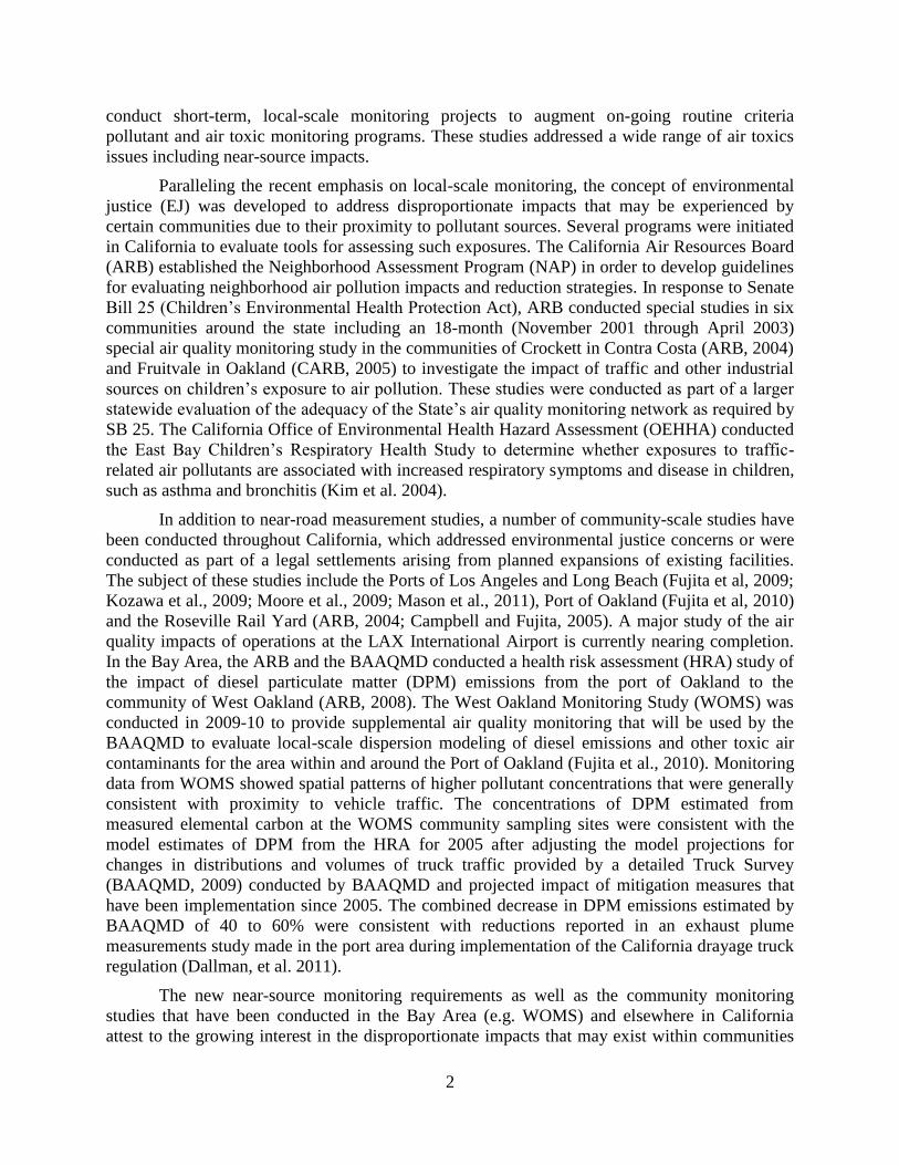
2

conduct short-term, local-scale monitoring projects to augment on-going routine criteria

pollutant and air toxic monitoring programs. These studies addressed a wide range of air toxics

issues including near-source impacts.

Paralleling the recent emphasis on local-scale monitoring, the concept of environmental

justice (EJ) was developed to address disproportionate impacts that may be experienced by

certain communities due to their proximity to pollutant sources. Several programs were initiated

in California to evaluate tools for assessing such exposures. The California Air Resources Board

(ARB) established the Neighborhood Assessment Program (NAP) in order to develop guidelines

for evaluating neighborhood air pollution impacts and reduction strategies. In response to Senate

Bill 25 (Children’s Environmental Health Protection Act), ARB conducted special studies in six

communities around the state including an 18-month (November 2001 through April 2003)

special air quality monitoring study in the communities of Crockett in Contra Costa (ARB, 2004)

and Fruitvale in Oakland (CARB, 2005) to investigate the impact of traffic and other industrial

sources on children’s exposure to air pollution. These studies were conducted as part of a larger

statewide evaluation of the adequacy of the State’s air quality monitoring network as required by

SB 25. The California Office of Environmental Health Hazard Assessment (OEHHA) conducted

the East Bay Children’s Respiratory Health Study to determine whether exposures to traffic-

related air pollutants are associated with increased respiratory symptoms and disease in children,

such as asthma and bronchitis (Kim et al. 2004).

In addition to near-road measurement studies, a number of community-scale studies have

been conducted throughout California, which addressed environmental justice concerns or were

conducted as part of a legal settlements arising from planned expansions of existing facilities.

The subject of these studies include the Ports of Los Angeles and Long Beach (Fujita et al, 2009;

Kozawa et al., 2009; Moore et al., 2009; Mason et al., 2011), Port of Oakland (Fujita et al, 2010)

and the Roseville Rail Yard (ARB, 2004; Campbell and Fujita, 2005). A major study of the air

quality impacts of operations at the LAX International Airport is currently nearing completion.

In the Bay Area, the ARB and the BAAQMD conducted a health risk assessment (HRA) study of

the impact of diesel particulate matter (DPM) emissions from the port of Oakland to the

community of West Oakland (ARB, 2008). The West Oakland Monitoring Study (WOMS) was

conducted in 2009-10 to provide supplemental air quality monitoring that will be used by the

BAAQMD to evaluate local-scale dispersion modeling of diesel emissions and other toxic air

contaminants for the area within and around the Port of Oakland (Fujita et al., 2010). Monitoring

data from WOMS showed spatial patterns of higher pollutant concentrations that were generally

consistent with proximity to vehicle traffic. The concentrations of DPM estimated from

measured elemental carbon at the WOMS community sampling sites were consistent with the

model estimates of DPM from the HRA for 2005 after adjusting the model projections for

changes in distributions and volumes of truck traffic provided by a detailed Truck Survey

(BAAQMD, 2009) conducted by BAAQMD and projected impact of mitigation measures that

have been implementation since 2005. The combined decrease in DPM emissions estimated by

BAAQMD of 40 to 60% were consistent with reductions reported in an exhaust plume

measurements study made in the port area during implementation of the California drayage truck

regulation (Dallman, et al. 2011).

The new near-source monitoring requirements as well as the community monitoring

studies that have been conducted in the Bay Area (e.g. WOMS) and elsewhere in California

attest to the growing interest in the disproportionate impacts that may exist within communities

3

that are located in close proximity to major emission sources. The fire that erupted at the

Richmond Chevron Refinery on August 6, 2012 heightened public concerns in the Bay Area

about such impacts and added impetus for the BAAQMD to consider additions or

reconfiguration of existing monitoring programs to inform susceptible communities of the

potential impacts of TAC emissions from major industrial sources.

Study Objectives

1. Identify the primary risk drivers that can be used to determine ambient air health risks

associated with living near refineries and chemical plants. While the main focus is on

emissions associated with normal plant operations, consider means to capture emissions

during plant upsets and accidents.

2. Review and evaluate current air monitoring capabilities.

3. Develop a matrix that lists additional instrumentation, methodologies and/or other

exposure assessment tools that could be employed to enhance monitoring capabilities and

provide information about emissions from refineries and chemical plants. Include in the

matrix potential advantages, disadvantages, and approximate costs associated with each

option that accommodate varying scales of the monitoring network.

4. Develop a short report describing the process used and how the matrix was developed.

Major Emitting Facilities in the Bay Area

The San Francisco Bay Area, the largest urban area in Northern California with

approximately 7.15 million people, encompasses the major cities and metropolitan areas of San

Francisco, Oakland, and San Jose, along with smaller urban and rural areas. The Bay Area's nine

counties are Alameda, Contra Costa, Marin, Napa, San Francisco, San Mateo, Santa Clara,

Solano, and Sonoma. The 2008 base year inventory in

4

Table 0-1 shows the contributions of areawide, mobile and stationary sources in the Bay

Area. Stationary Sources account for about 15% of the total emission of particulate matter less

than 2.5 µm (PM2.5), 28% of reactive organic gases (ROG), 11% of nitrogen oxides (NOx), 75%

of sulfur dioxide (SO2) and 3% of the carbon monoxide (CO).

Major emitting facilities are subsets of stationary sources that emit more than a total for

the facility of 0.05 tons/day of any criteria pollutant. The five refineries in the Bay Area account

for about half of the PM2.5, ROG and NOx emissions from all major emitting facilities and over

90% of the SO2 emissions.

5

Table 0-1 also shows the subcategories of emissions from petroleum refining and total

emissions of the five Bay Area refineries. The refineries are located in Contra Costa and Solano

County along the shore of San Pablo Bay and Suisun Bay. A list of the refineries, their location

and capacity is shown in Table 0-2. The aggregate emissions for industrial categories other than

petroleum refining are relatively small in comparison. The information in this report focuses on

refineries due to the greater potential for near-source impact in the Bay Area from this source.

However, the measurement method and approaches described in the report are generally

applicable to other point sources of hazardous air pollutants.

6

Table 0-1. Inventory of emissions (annual average tons per day) from petroleum refining in the

Bay Area.

PM10 PM2_5 ROG NOX SOX CO

Areawide 175.51 52.90 87.95 16.92 0.62 161.86

Mobile 20.33 16.27 183.12 380.52 14.93 1541.50

Stationary 16.30 12.14 106.58 50.59 45.95 44.31

Total Emissions 212.14 81.31 377.65 448.03 61.50 1747.66

Petroleum Refining

Catalytic Cracking 0.37 0.34 0.00 0.00 8.10 0.00

Coking 0.48 0.44 0.02 0.37 16.26 0.00

Cooling Towers 0.06 0.06 1.67 0.00 0.00 0.00

Fixed Roof Tanks 0.00 0.00 0.82 0.00 0.00 0.00

Floating Roof Tanks 0.00 0.00 1.67 0.00 0.00 0.00

Fugitive Losses 0.00 0.00 0.71 0.00 0.00 0.00

Others 0.02 0.02 0.17 0.07 0.04 0.06

Sulfur Plants 0.01 0.01 0.01 0.09 0.88 0.18

Tanks Unspecified 0.00 0.00 0.00 0.00 0.00 0.00

Vacuum Distillation 0.03 0.02 0.13 0.00 0.02 0.00

Vapor Recovery/Flares 0.00 0.00 0.03 0.08 0.33 0.03

Wastewater Treatment 0.00 0.00 0.94 0.00 0.00 0.00

Boilers 0.11 0.11 0.32 5.97 2.39 1.02

I.C. Reciprocating Engines 0.00 0.00 0.01 0.86 0.00 0.15

I.C. Turbine Engines 0.13 0.13 0.01 1.46 0.22 0.90

In-Process Fuel 0.08 0.08 0.43 0.66 4.22 2.61

Process Heaters 1.25 1.23 0.27 6.57 2.32 2.31

Total Petroleum Refining 2.57 2.45 7.20 16.11 34.78 7.26

% of Total Emissions 1.2% 3.0% 1.9% 3.6% 56.6% 0.4%

Major emitting facilities that emit more than 0.05 tons/day of any criteria pollutant.

All major facilities 8 6 19 33 38 36

Refineries

Chevron (Richmond) 0.62 0.55 2.80 2.26 4.65 1.50

Tesoro (Martinez) 0.42 0.28 3.14 4.48 7.75 0.88

Shell Oil (Martinez) 0.90 0.84 3.53 3.02 3.19 3.07

Valero (Bencia) 0.71 0.58 0.63 5.33 14.52 1.77

Conoco Phillips (Rodeo) 0.39 0.38 0.45 2.56 4.64 0.84

% of All Major Facilites 38% 44% 56% 53% 91% 22%

7

Table 0-2. Bay Area Refinery Locations and Capacities (Information as of October, 2012).

The Richmond Refinery is the largest and oldest (1901) major oil refinery on the West

Coast. With a processing capacity of over 350,000 barrels per day, this refinery is among the

largest in the United States. It covers 2,900 acres, has 5,000 miles of pipelines, and hundreds of

large tanks that can hold up to 15 million barrels of crude, gasoline, jet fuel, diesel, lube oil, wax,

and other chemicals produced by the refinery. Chevron is currently implementing an Air Quality

Monitoring program in the surrounding neighborhoods of North Richmond, Point Richmond and

Atchison Village. This program is part of the Richmond Community Benefits Agreement for the

Chevron Energy and Hydrogen Renewal Project. The Air Quality Monitoring Program will

sample air quality using testing methods similar to those used by government agencies and

publish these results on a community-accessible website.

The Martinez Refinery is the second largest refinery in the Bay Area and was the first

American refinery built by the Shell Oil Company in 1915. It is operated by Equilon, a joint

partnership of Shell and Texaco. Today it employs 900 people and processes around 165,000

barrels of crude per day. It is connected to oil fields in the Central Valley by a 170 mile long

pipeline.

The Golden Eagle Refinery in Martinez, also known as the Avon Refinery has a

processing capacity of 166,000 barrels of crude per day, making mostly automotive fuels. It was

built in 1913, to process heavy crude from the southern San Joaquin Valley, to which it is

connected by pipeline. It is now owned by Tesoro, of San Antonio, TX, and has previously been

owned by Tosco and Ultramar Diamond Shamrock.

The Benicia Refinery was built by Exxon from 1966-1969, and has the distinction of

receiving the first shipload of crude to be delivered from the Alaskan Pipeline, in 1977. Most of

the crude processed here still comes from the pipeline via Valdez, though the refinery is also

connected to a crude pipeline that brings oil from the San Joaquin Valley. It employs around 500

people, and is considered an average, large refinery, capable of processing 150,000 barrels of oil

per day. Exxon sold the refinery to Valero in 2000. The oil refinery and the surrounding

industrial park were built on the grounds of the Benicia Arsenal.

The San Francisco Refinery is an oil refinery located in Rodeo, California and in Arroyo

Grande, Califorina, in the San Francisco Bay Area and Santa Maria Valley. These two locations,

although more than 200 miles apart are considered one location. The two locations are directly

connected by a pipeline. The refinery is currently owned and operated by Phillips 66, a

downstream company with midstream and chemical businesses spun-off from ConocoPhillips in

2012. The complex is capable of refining 100,000 barrels (16,000 m3) of crude oil per day.

Refinery Name Location

Barrels

Per Day

Chevron U.S.A. Inc. Richmond Refinery Richmond 245,271

Tesoro Refining & Marketing, Golden Eagle Refinery Martinez 166,000

Shell Oil Products US, Martinez Refinery Martinez 156,400

Valero Bencia Refinery Benicia 132,000

Phillips 66, Rodeo San Francisco Refinery Rodeo 78,400

8

Refineries can be classified as topping, hydroskimming or complex. Topping refineries

are the least sophisticated and contain only the atmospheric distillation tower and possibly a

vacuum distillation tower. The topping refiner's ability to produce finished products depends on

the quality of the petroleum being processed. A hydroskimming refinery has reforming and

desulfurization process units in addition to basic topping units. This allows the refiner to increase

the octane levels of motor gasoline and reduce the sulfur content of diesel fuel. Complex

refineries are the most sophisticated refinery type and have additional process units to "crack"

the heavy gas oils and distillate oils into lighter, more valuable products. Complex refineries

have the highest utilization rate at approximately 95 percent. Utilization rate is the ratio of

barrels input to the refinery to the operating capacity of the refinery. Complex refineries are able

to produce a greater proportion of light products, such as gasoline, and operate near capacity.

The five refineries in the Bay Area are all complex refineries.

Chemical Species of Interest

Refineries emit a wide variety of pollutants including criteria pollutants (SO2, NOx, CO,

and PM), volatile organic compounds that are photochemically reactive (e.g., ethylbenzene,

formaldehyde), carcinogenic hazardous air pollutants (benzene, naphthalene, 1,3-butadiene,

polycyclic aromatic hydrocarbons), non-carcinogenic HAP (hydrogen fluoride, hydrogen

cyanide), persistent bioaccumulative HAP (mercury), and other pollutants (hydrogen sulfide).

Refineries include the following process units with associated air emissions.

Crude Desalting removes contaminants that can cause corrosion of equipment and

processing problems by washing the crude oil with water. Process produces wastewater

with contaminants including benzene and other VOCs that can be emitted into the air.

Control technology: steam stripper/biotreatment.

Catalytic Reforming converts naptha-boiling range molecules into higher octane

reformate. Process produces hydrogen as a byproduct that can be used in hydrotreaters or

the hydrocracker. Air emissions include CO, NOx, benzene, toluene, xylene,

naphthalene, other VOC and dioxins. Control technology: scrubber.

Fluid Catalytic Cracking upgrades heavier fractions into lighter, more valuable products.

Process uses a fluidized catalyst to contact the feedstock at high temperature and

moderate pressure to vaporize long chain molecules and break them into shorter

molecules. Largest source of emissions of SO2, NOx, CO, PM, and metals at the refinery.

Control technology: scrubber and ESP.

Sulfur Recovery removes and recovers H2S using an amine treating unit and the Claus

process. Air emissions include SO2, NOx, CO, carbonyl sulfide, and H2S. Control

technology: Scrubber.

Thermal Processing converts heavy fractions into lighter products. Types include delay

coking, fluid coking (no emissions), visbreaking (no emissions) and flexicoking (no

emissions). Heavy residues are thermally cracked in the delayed coking unit in a furnace

with multiple parallel passes (semibatch process), which cracks the heavy, long chain

hydrocarbon molecules into gas oil and petroleum coke. Process is potentially a

significant source of emissions. Delayed coking unit emits SO2, NOx, PM, HAP (metals)

and VOC. Control technology: Flares.

9

Flares are combustion control device used to burn waste gases in both normal and process

upset conditions. Flare stacks are primarily used for burning off flammable gas released by

pressure relief valves during unplanned over-pressuring of plant equipment. During plant or

partial plant startups and shutdowns, flare stacks are also often used for the planned combustion

of gases over relatively short periods. Oil refinery flare stacks may emit methane and other

volatile organic compounds as well as sulfur dioxide and other sulfur compounds, and soot

particles containing elemental carbon and polycyclic aromatic hydrocarbons (PAH).

Fugitive emissions are emissions of gases or vapors from pressurized equipment due to

leaks and other unintended or irregular releases of gases. Fugitive emissions are potentially the

largest source of VOC emission within a refinery. Leaks from pressurized process equipment

generally occur through valves, pipe connections, mechanical seals, or related equipment.

Fugitive emissions also occur from storage tanks. Because of the huge number of potential leak

sources and the difficulties in detecting and repairing some leaks, fugitive emissions can be a

significant proportion of total emissions. To minimize and control leaks at process facilities

operators carry out regular leak detection and repair activities. Routine inspections of process

equipment with gas detectors are used to identify leaks and estimate the leak rate in order to

decide on appropriate corrective action. Proper routine maintenance of equipment reduces the

likelihood of leaks.

Air Toxics Inventory

The Air Toxics "Hot Spots" Information and Assessment Act (AB 2588, Connelly, et.

al.1987: in the California Health and Safety Code § 44300,) established a formal regulatory

program for site-specific air toxics emissions inventory and health risk quantification that is

managed by California air districts. Under this program, a wide variety of industrial, commercial,

and public facilities are required to report the types and quantities of toxic substances their

facilities routinely release into the air. The goals of the Air Toxics Hot Spots Program are to

collect emissions data, to identify facilities with potential for localized health impacts, to

ascertain health risks, to notify nearby residents of risks that are determined to warrant such

notification, and to reduce significant risks. Table 0-3 gives the annual emission of HAP for the

five refineries in the Bay Area for 2009.

The Toxics Release Inventory (TRI) program was established in 1986 by the Emergency

Planning and Community Right-to-Know Act (EPCRA, section 313). In 1990, Congress passed

the Pollution Prevention Act (PPA), which required that facilities report additional data on waste

management and source reduction activities under TRI (Section 6607 of PPA). The Toxics

Release Inventory (TRI) is a database that contains detailed information on nearly 650 chemicals

and chemical categories collected from over 23,000 industrial facilities. The EPA maintains this

information in a national database called the Toxics Release Inventory, which is available to the

public via the Internet at www.epa.gov/tri. MyRight-To-Know TRI application

(http://www.epa.gov/tri/myrtk/index.htm) is a look-up tool on the web site, Table 0-4 summarize

the TRI data for the five refineries for the 2011 reporting year.

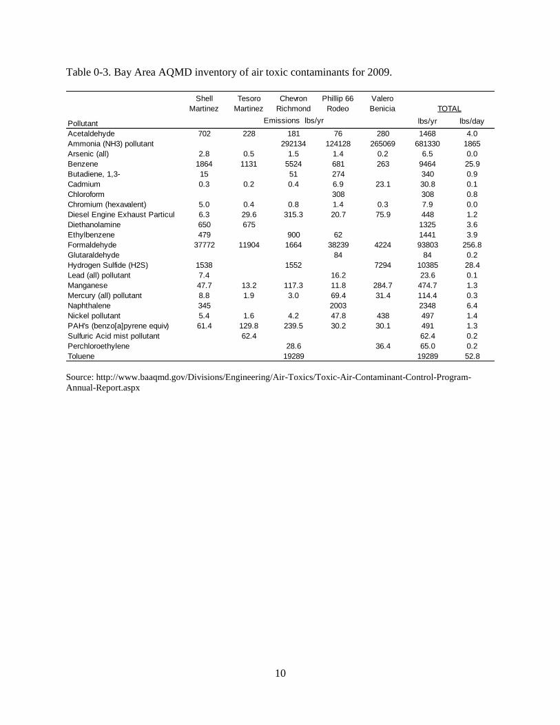
10

Table 0-3. Bay Area AQMD inventory of air toxic contaminants for 2009.

Source: http://www.baaqmd.gov/Divisions/Engineering/Air-Toxics/Toxic-Air-Contaminant-Control-Program-

Annual-Report.aspx

Shell

Martinez

Tesoro

Martinez

Chevron

Richmond

Phillip 66

Rodeo

Valero

Benicia

Pollutant lbs/yr lbs/day

Acetaldehyde 702 228 181 76 280 1468 4.0

Ammonia (NH3) pollutant 292134 124128 265069 681330 1865

Arsenic (all) 2.8 0.5 1.5 1.4 0.2 6.5 0.0

Benzene 1864 1131 5524 681 263 9464 25.9

Butadiene, 1,3- 15 51 274 340 0.9

Cadmium 0.3 0.2 0.4 6.9 23.1 30.8 0.1

Chloroform 308 308 0.8

Chromium (hexavalent) 5.0 0.4 0.8 1.4 0.3 7.9 0.0

Diesel Engine Exhaust Particul 6.3 29.6 315.3 20.7 75.9 448 1.2

Diethanolamine 650 675 1325 3.6

Ethylbenzene 479 900 62 1441 3.9

Formaldehyde 37772 11904 1664 38239 4224 93803 256.8

Glutaraldehyde 84 84 0.2

Hydrogen Sulfide (H2S) 1538 1552 7294 10385 28.4

Lead (all) pollutant 7.4 16.2 23.6 0.1

Manganese 47.7 13.2 117.3 11.8 284.7 474.7 1.3

Mercury (all) pollutant 8.8 1.9 3.0 69.4 31.4 114.4 0.3

Naphthalene 345 2003 2348 6.4

Nickel pollutant 5.4 1.6 4.2 47.8 438 497 1.4

PAH's (benzo[a]pyrene equiv) 61.4 129.8 239.5 30.2 30.1 491 1.3

Sulfuric Acid mist pollutant 62.4 62.4 0.2

Perchloroethylene 28.6 36.4 65.0 0.2

Toluene 19289 19289 52.8

Emissions lbs/yr

TOTAL

11

Table 0-4. 2011 Toxic Release Inventory (TRI) for refineries in the Bay Area in lbs per year.

Parameter Fugitive Point Fugitive Point Fugitive Point Fugitive Point Fugitive Point

1,2-DIBROMOETHANE 4 0

1,3-BUTADIENE 130 2 34 11 17 57 37 98

BENZENE 1600 2100 1954 1424 610 1200 1300 3200 3159 3334

CARBON DISULFIDE 0 1900 0 0 1 5 0 0 0 1472

CARBONYL SULFIDE 0 280 1359 0 5 0 0 0 0 9877

CHROMIUM 0 174 23 12 0 60

COBALT COMPOUNDS 2 4 0 71

CRESOL (MIXED ISOMERS) 40 440 1 11 2 20

CUMENE 100 260 280 170 117 11

CYANIDE COMPOUNDS 0 0 0 48 0 1452

DIETHANOLAMINE 80 0 1100 1 140 0

ETHYLBENZENE 2400 1400 630 721 1200 2700 830 750 2647 1710

HYDROCHLORIC ACID (1995 AND AFTER ACID AEROSOLS ONLY)0 2600 0 8900 0 0

LEAD COMPOUNDS 10 41 1 27 2 20 4 74 0 99

MERCURY COMPOUNDS 0.7 7.2 0.0 20.0 0.5 21.0 0.7 3.8 0.0 6.0

METHANOL 1700 28000 4715 0 0 22000 500 4100 0 59410

N-HEXANE 3200 10000 249 2295 1400 6700 2300 1500 47 1595

NAPHTHALENE 500 300 74 169 480 500 330 110 635 63

NICKEL COMPOUNDS 18 310 25 25 0 725

PHENOL 210 210 0 104 23 61 21 37

POLYCYCLIC AROMATIC COMPOUNDS 6.8 7.7 0.5 3.2 3.0 15.0 0.6 4.7 0.1 91.0

TETRACHLOROETHYLENE 2600 23 77 0 20000 0 52 2588

TOLUENE 8100 6000 4272 2516 3500 5700 2000 7000 10083 6365

XYLENE (MIXED ISOMERS) 9600 4400 4288 5696 4200 4200 2300 2800 11423 2282

Chevron, Richmond Phillips 66, Rodeo Shell Oil, Martinez Tesoro, Martinez Valero, Benicia

12

Health Risk Assessments

Table 0-5 shows the health risk values approved by the California Office of

Environmental Health Hazard Assessment (OEHHA) as of February 25, 2013 for toxic air

contaminants that are commonly associated with refinery emissions. By comparison, the unit risk

factor for diesel exhaust is 3.0 E-4 µg/m3. The table includes all cancer potency values and

noncancer acute, 8-hour, and chronic Reference Exposure Levels (RELs) that are available for

use in the AB 2588 Air Toxics "Hot Spots" Program. The most current acute and chronic health

values should be used for the development of a facility health risk assessment.

The BAAQMD conducted a risk assessment for refinery emissions as part of the

reformulated gasoline requirements in the 1990s. The results of this assessment are shown in

Table 0-6. Health risk results for the maximally exposed individual (MEI) have been adjusted

for changes in OEHHA health effects values (as of March 2012). The health risk impact for each

TAC calculated specifically for the MEI location were scaled by the ratios of the current and

previous health effect values. A recalculation of the health risk impacts using the updated health

risk values for all receptor locations may result in a change in the MEI location and a change in

the corresponding maximum risk values. This also doesn’t take into account any changes in the

facility’s operations since the Facility-wide HRA was prepared. TACs of most concern include

benzene, PAH, hexavalent chromium and 1,3-butadiene for cancer risk and nickel, H2S,

formaldehyde for acute risk.

13

Table 0-5. OEHAA health risk values as of February 25, 2013.

TAC

Oral Potency

Value

(mg/kg/day)-

1

Dermal Unit

Risk Factor

(ug/m3)-1

Soil Unit Risk

Factor

(ug/m3)-1

Mother's

Milk Unit Risk

Factor

(ug/m3)-1

Inhalation

Unit Risk

Factor

(ug/m3)-1

Total Unit

Risk Factor

(ug/m3)-1

Chronic

Inhalation

(ug/m3)

Chronic Oral

(mg/kg/day)

Maximum

Pathway

1/Chronic HI

(ug/m3) AEL ug/m3

1, 3- butadiene 1.70E-04 2.00E+01

Acetaldehyde 2.70E-06 1.40E+02 4.70E+02

Acrolein 3.50E-01 2.50E+00

Ammonia 2.00E+02 3.20E+03

Arsenic 1.50E+00 8.32E-03 4.05E-03 0.00E+00 3.48E-03 1.59E-02 1.50E-02 3.50E-06 3.97E-04 2.00E-01

Benzene 2.90E-05 6.00E+01 1.30E+03

Beryllium na 2.40E-03 7.00E-03 2.00E-03 6.99E-03

Bromine na na na naCadmium 4.20E-03 2.00E-02 5.00E-04 1.79E-02

Chlorine 2.00E-01 2.10E+02

Chlorobenzene 1.00E+03

Chromium, Hexavalent na 1.50E-01 2.00E-01 2.00E-02 2.00E-01

Copper na 1.00E+02

Cresols 6.00E+02Ethylbenzene 2.50E-06 2.00E+03

Ethylene Dibromide 7.10E-05 8.00E-01

Ethylene Dichloride 2.10E-05 4.00E+02

Formaldehyde 6.00E-06 9.00E+00 5.50E+01

Hexane 7.00E+03

Hydrochloric Acid 9.00E+00 2.10E+03

Hydrogen Cyanide 9.00E+00 3.40E+02

Hydrogen Sulfide 1.00E+01 4.20E+01

Lead 8.50E-03 6.96E-07 2.29E-05 0.00E+00 1.22E-05 3.58E-05 na naManganese 9.00E-02

Mercury 3.00E-02 1.60E-04 7.09E-03 6.00E-01

Methanol 4.00E+03 2.80E+04

Methyl ethyl ketone na 1.30E+04

Methyl tertiary butyl ether 2.60E-07 8.00E+03

Methylene chloride 1.00E-06 4.00E+02 1.40E+04

Naphthalene 3.40E-05 9.00E+00

Nickel 2.60E-04 1.40E-02 1.10E-02 1.40E-02 2.00E-01

Nickel Carbonyl (must adjust emissions for Ni portion only) 2.60E-04 1.40E-02 1.10E-02 1.40E-02 2.00E-01

Nitrogen Dioxide 4.70E+02

PAHs (as BaP) 1.15E+01 1.35E-02 2.02E-03 0.00E+00 1.01E-03 1.65E-02 na

Perchloroethylene 5.90E-06 3.50E+01 2.00E+04

Phenol 2.00E+02 5.80E+03

Selenium 2.00E+01

Styrene 9.00E+02 2.10E+04

Sulfur Dioxide 6.60E+02

Toluene 3.00E+02 3.70E+04

Xylenes 7.00E+02 2.20E+04

Zinc na na na

Derived Residential Cancer Risk for 0.02 g/s deposition

Derived Residential Chronic HI for 0.02 g/s

deposition

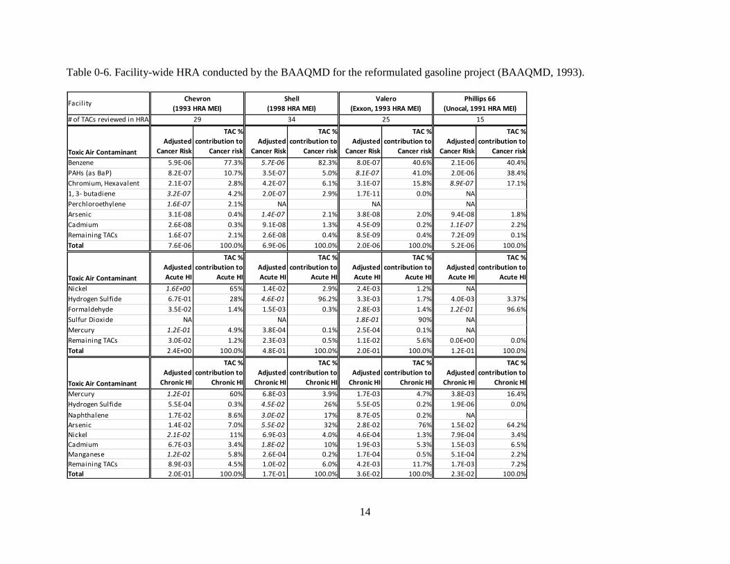
14

Table 0-6. Facility-wide HRA conducted by the BAAQMD for the reformulated gasoline project (BAAQMD, 1993).

Facility

# of TACs reviewed in HRA

Toxic Air Contaminant

Adjusted

Cancer Risk

TAC %

contribution to

Cancer risk

Adjusted

Cancer Risk

TAC %

contribution to

Cancer risk

Adjusted

Cancer Risk

TAC %

contribution to

Cancer risk

Adjusted

Cancer Risk

TAC %

contribution to

Cancer risk

Benzene 5.9E-06 77.3% 5.7E-06 82.3% 8.0E-07 40.6% 2.1E-06 40.4%

PAHs (as BaP) 8.2E-07 10.7% 3.5E-07 5.0% 8.1E-07 41.0% 2.0E-06 38.4%

Chromium, Hexavalent 2.1E-07 2.8% 4.2E-07 6.1% 3.1E-07 15.8% 8.9E-07 17.1%

1, 3- butadiene 3.2E-07 4.2% 2.0E-07 2.9% 1.7E-11 0.0% NA

Perchloroethylene 1.6E-07 2.1% NA NA NA

Arsenic 3.1E-08 0.4% 1.4E-07 2.1% 3.8E-08 2.0% 9.4E-08 1.8%

Cadmium 2.6E-08 0.3% 9.1E-08 1.3% 4.5E-09 0.2% 1.1E-07 2.2%

Remaining TACs 1.6E-07 2.1% 2.6E-08 0.4% 8.5E-09 0.4% 7.2E-09 0.1%

Total 7.6E-06 100.0% 6.9E-06 100.0% 2.0E-06 100.0% 5.2E-06 100.0%

Toxic Air Contaminant

Adjusted

Acute HI

TAC %

contribution to

Acute HI

Adjusted

Acute HI

TAC %

contribution to

Acute HI

Adjusted

Acute HI

TAC %

contribution to

Acute HI

Adjusted

Acute HI

TAC %

contribution to

Acute HI

Nickel 1.6E+00 65% 1.4E-02 2.9% 2.4E-03 1.2% NA

Hydrogen Sulfide 6.7E-01 28% 4.6E-01 96.2% 3.3E-03 1.7% 4.0E-03 3.37%

Formaldehyde 3.5E-02 1.4% 1.5E-03 0.3% 2.8E-03 1.4% 1.2E-01 96.6%

Sulfur Dioxide NA NA 1.8E-01 90% NA

Mercury 1.2E-01 4.9% 3.8E-04 0.1% 2.5E-04 0.1% NA

Remaining TACs 3.0E-02 1.2% 2.3E-03 0.5% 1.1E-02 5.6% 0.0E+00 0.0%

Total 2.4E+00 100.0% 4.8E-01 100.0% 2.0E-01 100.0% 1.2E-01 100.0%

Toxic Air Contaminant

Adjusted

Chronic HI

TAC %

contribution to

Chronic HI

Adjusted

Chronic HI

TAC %

contribution to

Chronic HI

Adjusted

Chronic HI

TAC %

contribution to

Chronic HI

Adjusted

Chronic HI

TAC %

contribution to

Chronic HI

Mercury 1.2E-01 60% 6.8E-03 3.9% 1.7E-03 4.7% 3.8E-03 16.4%

Hydrogen Sulfide 5.5E-04 0.3% 4.5E-02 26% 5.5E-05 0.2% 1.9E-06 0.0%

Naphthalene 1.7E-02 8.6% 3.0E-02 17% 8.7E-05 0.2% NA

Arsenic 1.4E-02 7.0% 5.5E-02 32% 2.8E-02 76% 1.5E-02 64.2%

Nickel 2.1E-02 11% 6.9E-03 4.0% 4.6E-04 1.3% 7.9E-04 3.4%

Cadmium 6.7E-03 3.4% 1.8E-02 10% 1.9E-03 5.3% 1.5E-03 6.5%

Manganese 1.2E-02 5.8% 2.6E-04 0.2% 1.7E-04 0.5% 5.1E-04 2.2%

Remaining TACs 8.9E-03 4.5% 1.0E-02 6.0% 4.2E-03 11.7% 1.7E-03 7.2%

Total 2.0E-01 100.0% 1.7E-01 100.0% 3.6E-02 100.0% 2.3E-02 100.0%

29 34 25 15

Chevron

(1993 HRA MEI)

Shell

(1998 HRA MEI)

Valero

(Exxon, 1993 HRA MEI)

Phillips 66

(Unocal, 1991 HRA MEI)

1

REVIEW OF EXISTING AIR QUALITY MONITORING NEAR REFINERIES

Air quality monitoring at and near the five refineries in the Bay Area include the

permanent and special purpose air quality monitoring stations operated by the BAAQMD, and

the ground-level monitors (GLM) that the refineries are required to operate as part of their permit

to operate. Additionally, the Phillips 66 (formerly Conoco Phillips) Rodeo Refinery and Chevron

Richmond Refinery are conducting additional fence line monitoring as part of an agreement with

the local communities. This section describes and summarizes the data from these measurement

programs and evaluates the adequacy of the existing monitoring for determining the impacts of

refinery emissions to air quality in nearby residential communities.

Criteria Pollutant and Air Toxics Monitoring by the BAAQMD

Ambient concentrations of criteria pollutants are routinely monitored in urban areas

throughout the country to determine compliance with National Ambient Air Quality Standards.

The National Air Monitoring Stations (NAMS) were established to ensure a long term national

network for urban area-oriented ambient monitoring and to provide a systematic, consistent

database for air quality comparisons and trend analysis. NAMS was replaced by the National

Core (NCore) network, which began in January 1, 2011 with 80 sites; 63 urban sites and 17 rural

sites. NCore is a multi-pollutant network that integrates several advanced measurement systems

for particles, pollutant gases and meteorology.

The State and Local Air Monitoring Stations (SLAMS) allow state and local governments

to develop networks tailored to their immediate monitoring needs. Special purpose monitors

(SPM) fulfill very specific or short-term monitoring goals and are typically used as source-

oriented monitors rather than monitors which reflect the overall urban air quality. Photochemical

Assessment Monitoring Stations (PAMS) are a specialized subset of SLAMS sites that collect

data on certain volatile organic compounds and carbonyl compounds (aldehydes and ketones) in

ozone nonatttainment areas. EPA has also developed additional specialized subsets for special

purposes, such as the Chemical Speciation Network (CSN) and National Air Toxic Trends

Stations (NATTS) discussed below.

Although the Clean Air Act does not require a national air toxics monitoring network,

many areas began sampling and analyzing ambient air samples for air toxics. Many of the high-

population states and local areas implemented their own air toxic monitoring programs including

California and the San Francisco Bay Area. Such s network was put in place by the BAAQMD in

1986. The EPA initiated a technical and laboratory analytical support program in 1988 to support

emerging needs for information regarding ambient levels of organic toxic species in ambient air.

This urban air toxic monitoring program (UATMP) supports the year-round collection and

analysis of a 24-hour canister sample every 12 days. EPA established the NATTS beginning in

1999 to provide long-term monitoring data for certain priority HAP across representative areas

of the country in order to establish overall trends for these pollutants. As of 2004, EPA had

established 23 NATTS in 22 cities. The national network is a subset of over 300 ambient air

toxics monitoring stations that have been established nationwide by State and local agencies. The

NCore monitoring station in San Jose (Jackson) is one of the NATTS.

EPA also established the CSN network to monitor and gather data on the chemical

makeup of PM2.5 (selected ions, metals, carbon species, and organic compounds) and to establish

the relationships between PM concentrations and public health impacts. The CSN (formerly the

2

Speciation Trends Network) was initiated by EPA in 2000. The CSN consists of 54 long-term

trends sites and approximately 185 supplemental sites. These sites are existing NCore and

SLAMS sites across the Nation. The BAAQMD air monitoring station in San Jose is also a CSN

as well as an NCore and NATTS site.

Routine Air Quality Monitoring Programs in the Bay Area

There are 27 air quality monitoring stations in the San Francisco Bay Area, 26 operated by the

BAAQMD and one operated by the California Air Resources Board (ARB). Twenty-three of the

27 stations are classified by EPA as SLAMS that are permanently sited. The remaining four are

classified as SPM stations in Crockett, Fort Cronkhite, Cupertino and Patterson Pass. The

BAAQMD also performs air monitoring as part the NATTS Program, the National Core (NCore)

Program, the PAMS Program, and the PM2.5 CSN Program. Table 0-7 lists the locations and

parameters measured at air quality monitoring stations in the Bay Area. The green highlights in

the Table indicate the eight monitoring stations that located within communities that are near the

five refineries. Five of the monitoring sites (Martinez, Point Richmond, Richmond 7th

, Rodeo

and Crockett) are intended to determine source impacts near the refineries. Three sites (Concord,

San Pablo, and Vallejo) characterize the pollutant concentrations in nearby urban areas. The map

in Figure 0-1 shows the locations of the eight BAAQMD monitoring stations (blue dots) and the

refinery GLM sites (yellow circles and triangles). The five refineries are shown on the map in

yellow strips and the white crosshatch show the populated urban areas of Contra Costa and

Solano Counties. Color-coded bars indicate the parameters measured at each of the BAAQMD

monitoring stations.

Figure 0-2 and Figure 0-3 show that, with the exception of Crockett, there are no

communities located downwind of the refineries during typical wind patterns.

The BAAQMD operates 18 air toxics monitoring sites. Locations are at existing SLAMS

and SPM monitoring stations and are generally in major population centers or downwind of

major industrial sources such as refineries. Air samples are collected for a 24 hour period on a 1-

in-12 day schedule except at special study sites such as Cupertino and San Jose where sampling

is on a 1-in-6 day schedule. Gaseous (VOC) toxics are collected in 6-liter SUMMA stainless

steel canisters using Xontech 910 samplers and analyzed by gas chromatography with

photoionization and electron capture detectors. Samples taken after January 1, 2012 were

analyzed using gas chromatography and mass spectrometry.

Summary of Existing Ambient Air Quality Data

The most complete extensively monitored pollutant of interest is SO2, for which hourly

measurements are recorded continuously at 9 sites (not including the GLM sites) to track

compliance with the NAAQS. As shown in Figure 0-4, although the 99th

percentile SO2

concentrations were higher at sites in communities near refineries than in San Jose, the

regulatory values measured were less than 10% of the primary and secondary standards at all

sites during 2011 and 2012. Interestingly, the highest mean SO2 concentrations occurred at the

San Pablo site in both years although it is located farther from the Chevron refinery than the

Richmond site. Such results illustrate the effect of prevailing wind patterns and the elevation and

buoyancy of pollutant emissions on the locations of greatest impact of refinery emissions.

3

The charts in Figure 0-5 and Figure 0-6 show the long-term trends in concentrations of

several gaseous HAPS over the last 12 years. The 90th

percentile for each year is plotted, to

represent the high-end of the concentration range and avoid the influence of outlier and below

detection values. A similar decreasing trend is seen for all sites, and the sites in communities

near refineries fall within the range observed at other sites in the Bay Area. Other VOC

compounds (ethylbenzene, o-xylene) were examined for the same time period, however most of

the values were near the limit of detection. Data for toxic metals is much more limited, but

Figure 0-7 indicates that concentrations are uniformly low relative to the OEHA recommended

chronic exposure limit (REL). The spatial distribution of formaldehyde and PAH could not be

evaluated since there are no sites near the refineries monitoring aldehyde or speciated organic

PM concentrations.

Existing Monitoring by Refineries

Ground Level Monitors (GLM) are air-quality monitoring stations that are required in the

permit conditions for certain large industrial facilities such as oil refineries. The facility operates

the monitoring equipment but the Bay Area Air Quality Management District audits and

validates the data.

In July of 1997, The Tosco Oil refinery in Rodeo, CA, USA (now owned by Phillips 66)

completed the installation of its new "fenceline monitoring system". This new monitoring

network, which incorporates ten optical remote sensing devices, is designed to detect and track

concentrations of a wide range of hazardous gases, and to provide early warning to the

surrounding communities in the event of a chemical emergency. Installation of the monitors

came about as part of an agreement reached between the refinery and local community groups in

after a disastrous chemical release which occurred in 1994 (UNOCAL facility at the time). After

this incident, Contra Costa County Health Services required additional air monitoring at the

refinery in conjunction with the refinery’s request for a land use permit. The County required the

refinery to work with community members to design and install a monitoring network that could

simultaneously measure and report toxic air pollutants at the refinery’s fenceline.

The refinery installed three types of open path monitors: FTIR (Fourier transform

infrared), UV (ultra violet), and TDL (tunable diode laser). The monitors sit along both the north

and south fencelines. Each of the monitors operates continuously, delivering data at 5-minute

intervals, 24 hours a day, 7 days a week. One monitoring station also collects meteorological

data, including wind direction. The FTIR measures ammonia, butane, carbon monoxide,

carbonyl sulfide, formaldehyde, methane, nitrous oxide, and ozone. The UV instrument monitors

for BTEX compounds (benzene, ethyl-benzene, toluene, and xylene). The TDL monitors

measure for ammonia and hydrogen sulfide. The data are available online at

http://www.ergweb2.com/fenceline/default.asp. The measurements at the concentrations reported

by the UV and TDL monitors are not sufficiently accurate that Contra Costa County is willing to

report them on this Web site. Current raw data from the fenceline monitors is posted by the

contractor, Argos Scientific, at www.fenceline.org along with messages describing events that

resulted in higher than normal level detection and links to data reports for the past few months.

Based on examination of the limited data available from this website, data for SO2 and BTEX are

generally below the 5 ppb LOD and the equipment has been frequently out of service.

Occasional concentration spikes were recorded, but most were determined to be due to

instrument calibration, weather events (fog), or false detections. Overall, it appears that the

4

system may be useful for early warning and evaluation of high-level releases and provides

information to the community about routine operation, but is not useful for determining

emissions flux during normal operations.

At the request of the City of Richmond, Chevron has agreed to implement an Air Quality

Monitoring Program in three neighborhoods surrounding the Chevron Richmond Refinery for

two years starting the second quarter of 2013. The locations are North Richmond, Point

Richmond and Atchison Village. Program will include fence line and community monitoring.

Monitoring measurements include: VOC, metals, H2S, PAH, and PM2.5, black carbon, ammonia,

and meteorological data. Fence-line monitors are proposed at the fence lines of each

neighborhood (3 total) and will be operated for a minimum of two years. Fence line

measurements will cover 1000 yards of fence line and measure benzene, toluene, xylene, SO2,

H2S and CS2. Fenceline data are now available online at

http://www.fenceline.org/richmond/data.php.

5

Table 0-7. Locations and parameters measured at air quality monitoring stations in the San Francisco Bay Area.

Notes: x = parameter monitored; P = parallel sampling with CARB; N = National Air Monitoring Station (NAMS); S = State and Local Air Monitoring Station

(SLAMS); CARB = CARB sampling only; C = collocated; F = FEM BAM.

STATION ADDRESS City / ZIP O3NOx Noy SO2

CO HC PM10

PM10

Continuous PM2.5

PM2.5

ContinuousTOXICS H2S

metals &

aldehyde PAH BC

PM2.5

SASS speciation

TSP

Lead

Neph light

scatter

PAMS

GC

UFP

Count

Hayward 3466 LaMesa Dr. 94542 X-S

Livermore 793 Rincon Ave. 94551 X-N X-S X X - F X X X X X X

Oakland 9925 International Blvd. 94603 X X X X - F X

Oakland 1100 - 21st Street 94607 X X X X X X X X

Pt. Richmond 140 W. Richmond Ave. 94801 X

Martinez 521 Jones St. 94553 X-S X

Crockett End of Kendall Ave. 94525 X-S X

Concord 2956-A Treat Blvd. 94518 X-N X-N X-S X-N X-N (2) X-C X

Richmond 1065 Seventh St. 94801 X-S X X

Bethel Island 5551 Bethel Is. Rd. 94511 X-S X-S X-S X-S X-S X

Rodeo 326 Third St. 94572 X

San Pablo 1865-D Rumrill Blvd. 94806 X-S X-S X-N X-S X X X

San Rafael 534 Fourth St. 94901 X-S X-S X-S X-N X - F X X

Fort Cronkhite Building 1049 94965 X

Napa 2552 Jefferson St. 94558 X-S X-S X-S X-S-C X X

San Francisco 10 Arkansas St. 94107 X-S X-N X-S X-N X - F X-P CARB

Redwood City 897 Barron Ave. 94063 X-S X-S X-S X - F X X X

Los Gatos 306 University Ave. 95030 X-N

Gilroy 9th & Princevalle Sts. 95020 X-S X - F

San Martin 13030 Murphy Ave. 95046 X-S

San Jose 158 E. Jackson St., Ste. B 95112 X-S X-N X-N X X-S X X X - F X-P X-N X-N X

Vallejo 304 Tuolumne St. 94590 X-S X-S X-S X-S X - F X X X

Fairfield 1010 Chadbourne Rd. 94534 X-S

Santa Rosa 837 Fifth St. 95404 X-S X-S X-S X - F X X

Cupertino 22601 Voss Ave. 95014 X X X X X X X X X

Patterson 6500 Patterson Pass Rd 94550 X X X

San Ramon 9885 Alcosta Blvd 94583 X X X

Palo Alto Airport 1925 Embarcadero Road 94303 X

San Carlos Airport 620 Airport Drive 94070 (2) X-C

Reid Hillview Airport 2500 Cunningham Ave 95148 X

TOTAL 21 16 1 10 13 2 7 1 3 12 18 3 3 1 2 4 4 4 3 4

6

Figure 0-1. Locations of active BAAQMD air monitoring sites and refineries in the Bay Area.

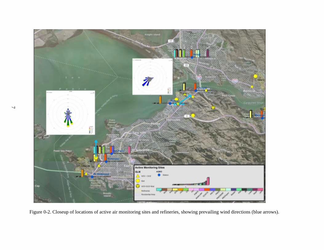
7

Figure 0-2. Closeup of locations of active air monitoring sites and refineries, showing prevailing wind directions (blue arrows).

8

Figure 0-3. Closeup of locations of active air monitoring sites and refineries, showing prevailing wind directions (blue arrows).

9

Figure 0-4. Annual statistics for SO2 sites in the Bay Area. The primary NAAQS is 75ppb (99th

percentile) and secondary is 500 ppb (maximum 3hr average).

10

Figure 0-5. Trends in air toxics, 2000 – 2012. Sites near refineries are indicated by bold black

lines. Values below LOD are not shown.

11

Figure 0-6. Trends in air toxics, 2000 – 2012. Sites near refineries are indicated by bold black

lines. Values below LOD are not shown.

12

Figure 0-7. Trend in fine particulate nickel, 2000 – 2012. Sites near refineries are indicated by

bold black lines. Values below LOD are not shown.

Incident Response Monitoring

Accidental releases of air contaminants trigger emergency response as specified by state

law. While emergency response agencies (state and local law enforcement and fire agencies)

have primary responsibility for scene management during an accidental release or emergency

incident, air pollution agencies can provide the following supporting resources: air sample

collection and analysis, air monitoring, dispersion modeling. The BAAQMD is responsible for

assessing the air quality impacts to the community and taking any enforcement action that may

be necessary based upon the cause of the accidental release.

Following an accidental release, such as the August 6, 2012 Chevron Refinery fire, the

Compliance and Enforcement Division of the BAAQMD prepares an incident report describing

the nature and cause of the incident and associated health alerts (available online at

http://www.baaqmd.gov/Divisions/Compliance-and-Enforcement/Incident-Reports.aspx). The

report summarizes the air quality data collected during the incident from nearby BAAQMD air

quality monitoring stations and facility GLMs along with air samples collected in downwind

areas. Protocols and procedures during such accidents are outlined in the BAAQMD Incident

Response Guidelines.

Special Studies

Special monitoring programs have been conducted in California to characterize the

ambient air toxic concentrations and potential exposures to certain susceptible populations and

within communities that may experience disproportionate impacts due to their proximity to

pollutant sources. The California Air Resources Board (ARB) conducted an 18-month

(November 2001 through April 2003) special air quality monitoring study in the communities of

Crockett in Contra Costa (ARB, 2004) and Fruitvale in Oakland (CARB, 2005) to investigate the

impact of traffic and other industrial sources on children’s exposure to air pollution. The studies

13

were conducted as part of a larger statewide evaluation of the adequacy of the State’s air quality

monitoring network as required by SB 25 (Children’s Environmental Health Protection Act).

Monitoring in the Crockett community was conducted at John Swett High School from October

2001 to May 2003.

Average levels of criteria air pollutants in Crockett were comparable to measurements

from the nearest long-term monitoring sites located in Vallejo and San Pablo. The average PM10

concentration at the Crockett site was 19 μg/m3 from October 2001 to May 2003 with a

maximum of 70 μg/m3. The State PM10 standard (50 μg/m

3) was exceeded on two occasions. The

State carbon monoxide, ozone and nitrogen dioxide standards were not exceeded during the

study. Monitoring of TACs included 1,3-butadiene, benzene, formaldehyde, acetaldehyde,

several halogenated compounds, polycyclic aromatic hydrocarbons and several metals. The

average concentrations of benzene and 1,3-butadiene during the monitoring period were 0.24 and

0.05 ppb, respectively and the corresponding cancer risks are 22 and 21 excess cancer cases in

one million people over a 70-year lifetime1, similar to the risks at the nearest long-term toxics

site, at Crockett. In general, the risk from toxic pollutants measured at John Swett High School

was approximately one-half of what was measured at Fremont..

Discussion and Conclusions

Exposures to hazardous air pollutants (HAP) within an urban area vary greatly due to

varying proximity to emission sources, magnitude and specific mix of emissions, and

meteorological conditions. These variations pose significant challenges for air quality monitoring

programs and the exposure assessments that rely on the available air quality data. The existing

air quality monitoring near the refineries are designed with the following objectives.

1. Determine community-scale average and range of concentrations for criteria pollutants

(SO2, NO2, CO) and certain high-priority HAP (benzene, toluene, ethylbenzene, xylenes,

1.3-butadiene, fomaldehyde).

2. Determine the impacts of routine and unplanned refinery emissions during unhealthy

levels of criteria pollutants or HAP.

This section reviews the measurement challenges and limitations of the existing monitoring

programs for addressing these objectives.

Five of the eight BAAQMD air quality monitoring stations that are located near or

downwind of the refineries are intended for monitoring source impacts. The San Pablo, Vallejo,

and Concord air quality monitoring stations are population-oriented monitoring sites, which are

designed to characterize air quality over neighborhood scales up to 4 km.

Point Richmond (H2S) is a source impact monitoring site located 300 m south of the

Chevron Refinery boundary. Although winds in the area are from the south-southwest,

occasional northerly winds will transport emission from the refinery over the community.

Richmond 7th

Street (SO2, H2S, toxics) is a source impact monitoring site located 0.8 km

east of the Chevron Refinery boundary, which is along the secondary prevailing wind

1 Cancer risk estimates in this report did not include diesel particulate matter (diesel PM).

14

direction. Prevailing northerly winds transport refinery emissions over the Bay to San

Pablo.

Rodeo (H2S) monitoring is a source impact monitoring site located 1.0 km southwest of

the Phillips 66 Refinery. This location is usually upwind of the refinery as the prevailing

winds are from the southwest.

Crockett (SO2, toxics) is a source impact monitoring site located downwind of the

Phillips 66 Refinery about 1.5 km northeast of the Phillips 66 Refinery and 300 m west of

I-80.

Martinez (SO2, toxics) is a source impact monitoring site located near downtown

Martinez and is 0.8 km southwest of the Shell Refinery and 4.0 km west of the Tesoro

Refinery. Prevailing winds in the area are easterly, putting the site downwind of the

refineries less than 3% of the time.

Vallejo (O3, NOx, SO2, CO, continuous PM2.5, speciated PM2.5, toxics) is a population-

oriented monitoring station in a mixed commercial and residential neighborhood 1.6 km

east of downtown Vallejo and 0.8 km west of Interstate 80. The site is about 4.8 km north

of the Phillips 66 Refinery and 8 km northwest of the Valero refinery.

San Pablo (O3, NOx, SO2, CO, PM10, continuous PM2.5, toxics) is a population-oriented

monitoring station located 1.9 km northeast of the Chevron Refinery. This area has heavy

industry and high traffic volume in addition to the Chevron Refinery, including two

major freeways.

Concord (O3, NOx, SO2, CO, PM10, continuous PM2.5, toxics) is a population-oriented

monitoring site in a residential area near the intersection of two major streets. Concord is

the largest city in Contra Costa County and is located in Diablo Canyon where locally

emitted pollutant can become trapped when wind are light. Large emission sources in the

valley include two major freeways and the Chevron and Tesoro Refineries located about

10 km to the north.

Various near-source air monitoring studies show that changes in pollutant concentrations

due to dispersion and dilution of emissions are inversely proportional to the square of the

distance from the source. This process of dilution can result in sharp gradients in pollutant

concentrations near sources of emissions. For example, NOx, CO and VOC concentrations near

major roadways typically drop from 2-4 times urban background levels at roadside to near the

surrounding urban background levels within 300 m downwind of the roadway (Zhu et al., 2002;

Fujita et al., 2003; Fujita et al., 2008, Fujita et al, 2010). Presence of diesel vehicles may increase

the near-road concentrations to as much as a factor of 10 higher than background for NOx and

black carbon (BC) (Fujita et al., 2010; Westerdahl et al. 2005). Even higher ratios have been

measured for NOx, sulfur dioxide (SO2), BC and ultrafine particles (UFP) near airport runways

during jet takeoffs (Westerdahl et al. 2008; Zhu et al., 2011).

With the exception of Pt. Richmond, which is located 300 m upwind of the Chevron

Refinery, all other monitoring sites are located 0.8 km or more from any refinery. Furthermore,

there are no communities located downwind of the refineries during typical wind patterns with

the exception of Crockett. The BAAQMD air toxic monitoring data show that the concentrations

of BTEX, 1,3-butadiene and perchloroethylene at the near-refinery monitoring locations are

generally lower than elsewhere in the Bay Area with similar long-term declining trends (2000-

15

2012) at all monitoring stations. These observations indicate that the urban background levels for

BTEX and 1,3-butadiene are primarily influenced by other emission sources, such as motor

vehicles, that are more evenly distributed throughout the Bay Area and produce greater total

emissions. Although SO2 can be considered a tracer for refinery emissions in the absence of

other significant sources in the area, all monitoring stations report similarly low SO2

concentrations throughout the Bay Area that are well below the NAAQS. Emissions from

process units are released from stacks, which result in elevated plumes of SO2, H2S and certain

VOCs that may travel some distance before reaching the ground. These emissions will add to the

regional background pollutant levels in downwind area with little impact to ground-level

concentrations near the refinery.

Data from the eight routine criteria and air toxics monitoring stations are generally

representative of the pollutant levels in the area and show no evidence of disproportionate

impacts from refinery emissions. However, for the reasons given above, they do not preclude the

possibility of higher concentrations at locations in closer proximity to the refinery and

consequential contributions to regional background pollutant levels further downwind (e.g.,

oxidation of SO2 to sulfate).

1

REVIEW OF AVAILABLE AIR MONITORING APPROACHES AND

MEASUREMENT METHODS

This section describes the air monitoring approaches that can be used to obtain air quality

data that can be used to determine the impact of refinery emissions on air quality in nearby

communities. The measurement options associated with these approaches are described.

Monitoring Approaches

Refineries are large facilities with multiple sources of process and fugitive emissions

scattered over a wide area. While process units produce emissions continuously from elevated

stacks, fugitive emissions (e.g., valves, pumps, connectors, storage tanks) have multiple sources

with varying chemical composition and temporal patterns. As a result, the concentrations and

mix of pollutants are temporally and spatially irregular with potentially complex vertical

variations in pollutant concentrations at the boundaries of refinery. Unlike vehicle emissions, the

chemical composition of refinery emissions indicated by the emissions inventory does not exist

and cannot be directly measured. Consequently, no single pollutant can serve as a tracer or

surrogate for other refinery emissions. Measured ambient concentrations of SO2 or H2S alone do

not necessarily imply the presence of other emissions from the refinery such as benzene or

metals, nor their attribution to refinery emissions. Facility-specific health risk assessments

(HRA) are typically performed by applying risk factors to predicted pollutant concentrations

obtained from by dispersion modeling. Dispersion modeling results provide useful insight

regarding the spatial distributions of pollutant concentrations in downwind areas where

monitoring data are not available. However, the reliability of the modeling results depend on the

accuracy of the emission inventory estimates. Based upon a review of existing monitoring

programs in the previous section, we identify the following measurement approaches that could

provide useful data for assessing the impact of refinery emission on air quality in nearby

communities.

Emission Flux Measurements

A number of studies in the U.S., Canada and Europe have found that reported emissions

of volatile organic compounds (VOCs) at refineries and chemical plants are substantially

underestimated (Cuclis, 2012). Techniques such as Differential Absorption Light Detection and

Ranging (DIAL) and Solar Occultation Flux (SOF) measure the VOC concentrations in a two

dimensional vertical plane and calculate VOC flux in pounds per hour. The results determine the

total VOC mass released.

DIAL makes use of pulsed lasers which reflect off particles in the air to provide

information about pollutant concentration. Typically these lasers are scanned across a vertical

plane perpendicular to the wind direction. A two dimensional concentration map is constructed

and used in conjunction with the perpendicular wind speed to measure the mass flux of

emissions. All DIAL vendors who take measurements at petrochemical facilities currently are

based in the U.K. According to recent estimates, the cost of the measurement techniques can

easily exceed $500,000 for a one-month study and the cost of a new DIAL system is typically at

least $2-3 million (Cuclis, 2012).

2

SOF uses a Fourier Transform Infrared (FTIR) spectrometer mounted in a passenger van.

As the van drives past a petrochemical complex on a sunny day, it gathers information about the

concentration of chemical species and a background subtraction is applied using readings taken

before and after approaching the petrochemical facilities. This information is combined with

wind direction and speed to calculate the mass flux of pollutants. The cost for a one-month study

can up to $200,000 and a new SOF unit may be built for $400,000 -$500,000; however, issues

relating to purchasing or licensing the SOF technology must be resolved with the developer

(Cuclis, 2012)..

Emission Plume Characterization

Optical remote sensing (ORS) utilizes a light source to detect and measure concentrations

of chemical compounds along the distance covered by the light signal. Depending on the source

of light (wavelength), the following types of ORS instrumentation could be used:

Open-Path Fourier Transform Infrared Spectrometer (OP-FTIR), IR light, 2 to 20

micrometers wavelength

Open-Path Tunable Diode Laser Absorption Spectrometer (OP-TDLAS), near-IR light,

approximately 1.5 micrometers wavelength

Ultraviolet Differential Absorption Spectrometer (UV-DOAS), UV light, 245 to 380

nanometers wavelength

Optical remote sensing (ORS) instruments have been used as an alternative to

conventional point monitors for measuring air emissions for many years. ORS instruments use

infrared (IR), laser, or ultraviolet (UV) light to measure concentrations of chemical compounds

of interest along the distance covered by the light signal. A light signal is sent out to mirrors

deployed in the field, and the signal is reflected back to the instrument detector. Depending on

the instrument and application, typical ORS instrument range varies from 50 to 500 meters. The

major advantage of ORS instrumentation over traditional point monitors is their ability to

provide greater spatial resolution of the monitored area. The increased resolution reduces the

chance of emissions hot spots being undetected over the measured area. It is possible to

accomplish increased spatial resolution because of the development of the Radial Plume

Mapping method (RPM), which is capable of collecting concentration data along multiple beam

paths in the configuration. In this method, multiple retro-reflecting mirrors are deployed in the

survey area. The RPM can be applied using any scanning ORS instrument.

Community Air Monitoring

The characterization of a community’s exposure to air pollutants is essential in assessing

cumulative health impacts. However, the costs of traditional monitoring technologies pose

significant limitations on the number of monitoring locations that can be established for exposure

studies. A few widely-spaced fixed monitoring stations have limited capacity to characterize

3

localized high concentrations and accompanying sharp pollutant concentration gradients that

may exist near emission sources. Yet various measurement and modeling studies and

epidemiological evidence indicate that such high concentrations with sharp concentration

gradients are critically important to characterize in order to accurately determine human

exposures and possible adverse health effects at the individual and sub-community levels.

The term “saturation monitoring” is used in reference to ambient air monitoring for the

purpose of establishing more detailed spatial variations in pollutant concentrations at the

community scale. The objectives of this type of monitoring in the context of health risk

assessments is to determine the seasonal or annual average air toxics concentrations at a

sufficient number of locations within the community to: 1) establish the spatial variations in

annual average pollutant concentrations; 2) identify the potential influence of hotspots of

pollutant emission on the community’s exposure; and 3) characterize gradients in pollutant

concentrations from these hotspots. Besides the accuracy, precision, selectivity and sensitivity of

alternative measurement methods, the range of sampling periods, power requirements, size and

portability of sampler or instrument are important considerations in a saturation monitoring

study. The Desert Research Institute recently conducted saturation monitoring as part of the

Harbor Community Monitoring Study (HCMS) (Fujita et al. 2009) sponsored by the California

Air Resources Board and the West Oakland Monitoring Study (WOMS) (Fujita et al. 2010)

sponsored by the Bay Area Air Quality Management District, and the Barnett Shale Gas

Production Study (Zielinska et al, 2010). The same approach has been applied in on-going LAX

International Airport Air Quality and Source Apportionment Study (AQSAS). The core

component of the saturation monitoring networks consisted of 7-day time-integrated sampling at

multiple sites using a combination of passive diffusive samplers for NO2, NOx, SO2, H2S, VOC

(benzene, toluene, xylenes, ethylbenzene), and carbonyl compounds (formaldehyde,

acetaldehyde and acrolein), and mini-volume aerosol sampling for PM2.5 mass, elements and

organic and elemental carbon and metals. Samples were collected during 28 to 42 consecutive

days in 2 or 4 seasons. This approach maximizes the number of sampling sites with the resources

available while providing sufficient data to determine valid annual average ambient

concentrations of TACs at each site. These time-integrated measurements are supplemented by

continuous measurements of CO, NOx, SO2, and PM at existing air quality monitoring stations.

Saturation monitoring provides spatial information about cumulative exposure

concentrations over an extended period of time. To address possible acute health effects, the

saturation monitoring is coupled with a smaller network of air monitoring stations that provide

time-resolved gaseous pollutant and PM mass concentrations. A complementary approach is the

use of a mobile platform equipped with real-time and near real-time monitoring instruments that

provide the necessary time resolution to identify high concentrations and sharp spatial gradients.

Continuous Monitors

Continuous monitoring methods provide the time resolution necessary to correlate

variations in pollutant concentrations with temporal patterns of source activity. They also allow

the flexibility to examine pollutant concentrations averaged over different time scales, which can

be useful for evaluating potential acute and chronic health impacts to a community.

4

Fixed-site Gas Analyzers

This type of monitor is typically used monitoring of criteria gaseous pollutants, and

accepted methods have been designated by EPA for regulatory purposes. They are designed to

operate continuously for years with minimal maintenance, but require a weatherproof shelter

with temperature control and periodic evaluation of the zero level and gain by introduction of

clean air and an appropriate gas standard (span gas).

Nitrogen Oxides

Nitric oxide (NO) is continuously measured by the chemiluminescence nitric oxide-ozone

method (OCM). This method is based on the gas-phase chemical reaction of NO with ozone. In

this method ambient air is mixed with a high concentration of ozone so that any NO in the air

sample will react, releasing photons in the process. The resulting light intensity is measured with

a photomultiplier and converted into an electronic signal which is proportional to the NO

concentration. To measure NOx concentrations, the sum of NO and NO2 (nitrogen dioxide), the

NO2 in the air sample is first reduced to NO, either by a heated catalyst (molybdenum or gold in

the presence of CO) or chemically using FeSO4, adding to the NO already present in the sample,

then introduced into the reaction chamber for measurement as described above. The NO2

concentration is derived by subtracting the NO concentration measurement from the NOx

concentration measurements. Monitors typically cycle through the total NOx and NO modes

every 10 seconds.

Standard sensitivity instruments have detection ranges from ≤0.5 ppb to 20 ppm and

response times < 60 seconds, and are suitable for air quality monitoring in urban and suburban

areas. Thermo Environmental Instruments, Inc. (TEI) Model 42i and Ecotech 9841 are examples

of this type of instrument. These have been used widely by federal, state, and local agencies for

routine monitoring of NO and NO2.

The reduction of NO2 to NO by these methods is not specific and a number of other

nitrogen-containing species are reduced to NO that can interfere with the measurement of NO2

(e.g., HNO3, PAN, N2O5, HONO, and NO3). Since the group is not well defined, it is commonly

referred to as NOx and the species included in the group depend on factors such as inlet and line

losses and environmental factors. HNO3 is most prone to line losses. Placing the converter as

close to the sample inlet as possible minimizes these losses. Chemiluminescence analyzers that

are configured in this manner are commonly known as NOy analyzers. NOy, or reactive

nitrogen oxides, consists of a variety of species, the most abundant of which are typically NO,

NO2, PAN and HNO3. TEI Model 42i-Y and Ecotech 9843 are commercially available NOy

analyzers.

Sulfur Dioxide

Analyzers like the Thermo 450i and Ecotech 9850 use UV fluorescence detection

technology to measure SO2 in ambient air with detection limits and response times similar to the

NOx analyzers. The Thermo 450i can also convert H2S to SO2, allowing differential

measurement of H2S in a manner analogous to the NO2 method described above. Increased

sensitivity can be achieved by trace-level analyzers like the Thermo 43i-TLE, which is designed

to measure concentrations down to 50 ppt. Since ambient levels of SO2 are frequently below 1

ppb in many areas, this extra sensitivity may be required to accurately monitor average

concentrations.

5

Carbon Monoxide

CO is typically monitored by absorption of IR light using the gas-filter correlation

method, in which a rotating filter wheel containing a known concentration of CO passes in front

of the beam at regular intervals. Because infrared absorption is a nonlinear measurement

technique, it is necessary for the instrument to use this reference signal to transform the detector

signal into a linear output relative to the concentration of CO in the sampled air. Detection limits

of 40 ppb are achieved in this manner, with range up to 200 ppm or greater.

VOC

Automated gas chromatographs (GC) can provide speciated analysis of gaseous organic

compounds in ambient air over discrete time intervals as short as 15 minutes. The analytical

method is analogous to that used to analyze canister samples in a laboratory with a GC/FID

(Flame Ionization Detector) system and can detect individual compounds <1 ppb. Although

automated, these instruments consume hydrogen gas and zero air and require appropriate span

gas blends for calibration standards.

Total HC or VOC concentrations can be continuously monitored using FID or PID

(Photo Ionization Detector), but provide no speciation information. The Thermo 55i monitors

non-methane hydrocarbons (NMHC) down to 50 ppb with a response time of <90 seconds. PID

based monitors such as the Rae Systems ppbRAE 300 can record continuous HC levels down to

ppb levels without the requirement for any zero or carrier gas, but the response to different types

of compounds varies so the result is only semi-quantitative for air containing a mixture of

organic compounds.

Open-Path Gas Monitors

Although fixed site monitors can provide high sensitivity and time resolution, they may

be inadequate to monitor pollutant concentrations that vary spatially due to proximity to a source

or complex terrain. An alternative that is less sensitive to localized variations in concentration,

but can still provide high time resolution, is to use open-path optical methods. These systems

measure the attenuation of light of specific frequencies due to absorption by various pollutants.

The performance achieved by open-path monitors is highly dependent on configuration of the

optical components (path length, alignment), atmospheric conditions (dust, smoke, fog, or

turbulence), and interferences from high concentrations of gases other than those of interest.

Detailed information on the various technologies for open-path monitoring can be found in the

EPA Handbook: Optical Remote Sensing for Measurement and Monitoring of Emissions Flux

http://www.epa.gov/ttnemc01/guidlnd/gd-052.pdf so only a brief description of the relevant

features is given here.

OP-FTIR (Fourier Transform Infra-Red)

The most commonly used open path systems employ a long wavelength light source that

has characteristic absorption bands for many organic compounds plus CO and SO2. Since the

relationship between concentration and absorption of IR light is a non-linear function, a library

of absorption spectra and Fourier transform signal processing are used to produce a linear output

for the compounds of interest. As a result of the intensive data processing required, a subset of

the hundreds of possible species is typically reported.

6

Open path FTIR systems can be installed in 3 basic configuratons: Bistatic in which a

separate light source is directed at the receiver, Monostatic in which the light source originates at

the detector and is reflected back by a mirror, and Passive in which only ambient radiation is

received by the detector. The highest sensitivities are achieved by the bistatic configuration, but

it requires electric power and operator access at both ends of the path. Monostatic systems give

up some sensitivity for a simpler configuration and more flexible siting (e.g. reflector may be

mounted on a stack or tower to give a vertical component to the measurement path). Passive

systems require less power and can easily be repositioned, but have low sensitivity and can only

detect flares or hot plumes at night. Path lengths may be up to 1000 meters with bistatic systems

and cryogenically cooled detectors, but 100 meter paths are more typical.

DOAS

Differential Optical Absorption Spectroscopy systems are similar in concept to bistatic

OP-FTIR, but may use short wavelength UV light sources to achieve higher sensitivity for NO2,

SO2, and some organic species such as benzene. As with FTIR, a selected set of species is

reported but some systems can store the raw spectra for later reanalysis if additional species are

desired.

Imaging systems

A variety of remote sensing techniques exist for identifying and characterizing emissions.

IR Cameras

Video cameras tuned to IR wavelengths that are absorbed by methane and hydrocarbons

(HC) (FLIR GF300) can be used to identify the location of emissions in real-time. Spectral

imaging devices designed to be deployed at fixed locations for remote identification and

characterization of gas plumes are available from Bruker (HI 90, SIGIS 2).

DIAL

Differential Absorption Lidar can create images of the flux of gaseous species across a

facility boundary. The technique measures the backscattered intensity of light at different UV-

VIS-NIR wavelengths while scanning in a 2-dimensional plane. The resulting data can be used to

quantitatively characterize emissions or track plumes.

DIAL systems are large and complex, and require specially trained operators, so they are

only suited to short-term studies to characterize emissions rather than routine monitoring.

SOF

A technology similar to DIAL that is used for annual emissions evaluations in parts of

Europe is Solar Occultation Flux, in which a spectrometer mounted in a vehicle tracks the sun as

it moves across a transect near a facility. SOF can quantify the flux of NO2, SO2, or specific

VOC compounds (FluxSense AB, Sweden).

PM Mass Monitors

Beta Attenuation

Beta particles are absorbed by matter at a rate that is proportional to the areal mass density.

By collecting aerosol particles on a filter tape that passes between a radiation source and beta

detector, the accumulated mass of particles can be derived from the increase in attenuation of the

7

beta source. This method is not truly continuous since it calculates mass concentrations from the

change in signal relative to a baseline measurement from a clean section of filter tape at regular

intervals, typically 1 hour. Although not a direct mass measurement, beta attenuation has been

sufficiently validated to be accepted as a Federal Equivalent Method (FEM) and is widely used

in regulatory monitoring for the PM2.5 and PM10 air quality standards. Since the method

calculates aerosol concentrations from the very small increase in density of a spot on a filter tape

(typically a glass fiber matrix) over a fixed time period (1 hour), there is a large uncertainty in

the individual hourly measurements (±10 μg/m3), however longer averaging times decrease the

uncertainty (±2 μg/m3 for 24 hrs). As with any on-site mass measurement, humidity can affect

the measured concentration so these monitors are generally operated with a heated inlet to

maintain sample RH below a predetermined level (typically 45%)

Variations on the standard FEM beta attenuation monitor (e.g. MetOne BAM) may provide

better temporal resolution. The Thermo SHARP monitor incorporates a light-scattering sensor

along with the beta detector. The light-scattering signal, which is more sensitive but dependent

on aerosol composition and morphology is used to track short-term variations in concentration

during hourly beta-attenuation measurements. Kimoto makes a monitor that uses Teflon

membrane tape, which has a much lower density than glass fiber, to reduce the uncertainty of the

beta-attenuation measurement. The Kimoto monitor is also equipped for use with an optional

separator tape that protects the sample deposits as they are rolled onto the take-up spool so that

they may be preserved for compositional analysis.

The subsequent analysis of tape sampler spots by XRF to determine the elemental composition

of aerosol during events of interest has been successfully demonstrated by Watson, et al. (2012)

for the FEM type BAM sampler, although reduced sensitivity due to the media thickness and

some loss of material due to contact with the back of the adjacent tape roll was noted. Analysis

of sample spots from PTFE tape should allow improved analysis results, however the Kimoto

instrument is produced in Japan and not widely used in the US limiting the available information

about its suitability for routine monitoring. . Modification of the BAM or EBAM to use Teflon

tape is available from MetOne on request, and might be a better option if those monitors are

already in use in the network.

TEOM

The TEOM utilizes a unique method for measuring aerosol mass concentrations. Particulate

matter is actively collected onto a small filter mounted on the tip of a vibrating glass cone.

Increases in the mass on the filter change the resonant frequency of the cone, and this variation is

detected and translated to mass concentration. This “oscillating microbalance” method is quite

sensitive, but requires precise control of the instrument temperature and flow rates making the

TEOM more expensive and complex than other continuous mass methods. While the TEOM

incorporates a heated inlet to control sample air humidity, it has been our experience that it can

produce highly erratic readings when ambient RH changes rapidly such as during daily fog

events, so it is not recommended for this program.

8

XRF Tape Sampler

A unique type of analyzer that can provide continuous elemental analysis of aerosol particles

is marketed by Cooper Environmental. The Xact 625 and related models collect aerosol on a

filter tape in a manner similar to a beta-attenuation sampler, however an X-ray fluorescence

source and detector provide detailed elemental analysis (K to Pb) of the filter deposit with time

resolution as short as 15 minutes. Detection limits below 1 ng/m3 are possible for most metals.

As with any filter based analysis method, actual performance will vary with composition and

density of the aerosol deposit. The Xact has the potential to characterize the temporal variations

of toxic metals for evaluation of potential acute health effects, but the high cost (approx. $250k)

and complexity of the instrument would likely prevent its use at multiple monitoring locations.

Nephelometers

Aerosol mass concentrations can be estimated from the scattering of light by particles. This

nephelometry approach is used in a variety of “real-time” monitors, such as the TSI DustTrak or

MIE DataRAM. While such monitors can provide good sensitivity and very fast response times,

the relationship between light-scattering and mass concentration varies significantly with

changes in aerosol composition, size distribution, hydration, and morphology so observed

fluctuations in reported mass concentration may be due, all or in part, to other factors. For

example, during one prior study mass concentrations reported by the DustTrak were found to

exceed gravimetric mass concentrations for mobile ambient samples by a factor of 2.24 with an

R2 of 0.75. For this reason, we would not recommend relying on light-scattering except as an

adjunct to more direct mass measurement methods with less time resolution.

Black Carbon Monitors

Light-absorbing carbon, also referred to as black carbon (BC) and elemental carbon (EC), is

a product of fuel combustion and has been used as a viable surrogate for estimating ambient

concentrations of “diesel particulate matter” (DPM), in areas where diesel vehicle exhaust is

known to be the dominant source of EC. Two commercially available methods that have been

used to monitor BC with fast time resolution are the Aethalometer and the photoacoustic aerosol

spectrometer.

The Aethalometer collects aerosol particles on a filter tape and measures the decrease in

transmittance of light thru the tape as it becomes progressively darkened by the light absorbing

particles in the air stream. An empirically developed algorithm is used to convert the measured

changes in transmittance over time to concentrations of BC. The technique is quite sensitive,

providing detection limits well below 1 µg/m3, and the use of multiple wavelength light sources

can provide some information about the composition of the light-absorbing particles. However,

the effect of light scattering by particles can cause a well-documented non-linear response2,3

when aerosol concentrations are high, resulting in significant underestimation of BC

concentrations.

The photoacoustic instrument was developed at DRI and has been described in several

publications (Arnott, Moosmüller et al. 1999; Arnott, Moosmüller et al. 2000). Briefly, light

2 California Energy Commission (2007), Evaluating Past and Improving Present and Future Measurements of Black

Carbon. 3 Weingartner, et al. (2003), Absorption of Light By Soot Particles: Determination of the Absorption Coefficient by

Means of Aethalometers. Journal of Aerosol Science, 34:10.

9

from a 1047 nm laser is power-modulated at the operating frequency of an acoustical resonator.

Sample air is continuously drawn through the resonator at a flow rate of 1 – 3 lpm. Light

absorbing aerosol (black carbon) will absorb some of the laser power, slightly heating the aerosol

(typically much less than 1 C). The heat transfers very rapidly from the aerosol to the

surrounding air, and the local pressure increases, contributing to the standing acoustic wave in

the resonator. The acoustic wave is measured with a microphone as a measure of the light

absorption. For the operating conditions of the resonator, and the laser wavelength used, the light

absorption measurement is linearly proportional to the mass concentration of the black carbon

aerosol in the sample air. The constant of proportionality has been inferred from correlations of

black carbon measurements with elemental carbon as determined by the TOR method, and is

used to go from aerosol light absorption to estimated black carbon mass concentration. No filters

are needed for the photoacoustic measurement, and the flow rate is not used in the calculation of

aerosol mass concentration. The flow rate must only be sufficient to adequately sample the air

with minimal particle loss in the instrument and sample lines. The resolution of the instrument

for a 3 second averaging time is 0.5 microgram per cubic meter for black carbon mass

concentration. The resolution scales as the square root of sampling time, so for example, a

resolution of 0.25 micrograms per cubic meter can be obtained for a 9 second averaging time.

The photoacoustic measurement does not receive interference from exhaust gases, in our

experience so far, and it is a zero-based measurement when no light absorbing aerosols are

present. Commercial versions of the instrument, providing measurements of BC and total mass

concentrations (estimated from light scattering) at multiple wavelengths, are available from

Droplet Measurement Technologies.

PAH monitor

The Ecochem PAS 2000 is a photoelectric aerosol sensor (PAS) for continuous measurement of

particle-bound polycyclic aromatic compounds (PAH). According to the manufacturer, it

measures 3 or more ringed PAH which are predominantly adsorbed on particles and also pose

the maximum health risk. Sensitivity is in the ng/m3 range and the instrument is portable with a

built in pump with flow control, datalogger, and serial output.

The PAS has been characterized and applied during the past couple of decades by various

investigators. The PAS response varies for different PAHs and must be calibrated to appropriate

mixtures of PAHs if these monitors are to provide more than semi-quantitative screening

estimates of PAH exposure. Exposing the PAS to high levels of water vapor or source emissions,

such as diesel exhaust, can cause erratic results. PAS results have also been found to vary with

inlet temperature. However, the question about what the PAS really measures goes beyond

calibration. The morphology of particles emitted from combustion sources changes rapidly due

to adsorption of semi-volatile material on the particle surface and due to coagulation. These

processes are important to the question of what the PAS measures since only surface

composition contributes to the photoemission signal (Niessner et al, Anal. Chem. 1990, 62,

2071-2074). Because of these issues, data from the PAS may only be considered semi-

quantitative in most situations. Therefore, its benefit for exposure estimates may be limited to

qualitative source attribution when combined with other compositional data such as BC

concentrations.

Ultrafine Particle Counters

10

Also known as Condensation Particle Counters, CPCs measure particle number

concentrations by supersaturating an incoming air stream with a condensing liquid and thereby

growing smaller particles to a size at which they can be detected optically. There are a variety of

models available from TSI and other vendors, that differ mainly in the condensing liquid used

(butanol, isopropanol, or water) and the resulting ability to detect particles below 10 nm size.

They typically record particle number concentration data with 1-minute or faster time resolution.

Since aerosol size distributions are typically dominated in number by the smallest particle sizes

and change rapidly with distance from combustion sources, the low-end sensitivity and accuracy

of an individual instrument to these nm sized particles and the can greatly influence the

measured particle counts making UFP data difficult to compare between monitors. Since these

instruments provide no information about the size distribution or composition of the particles

counted it is not possible to convert the measured number concentrations to mass concentration

equivalent or estimate potential health effects.

Time-Integrated Gaseous Speciation Sampling and Analysis

Not all gaseous pollutants can be monitored continuously with sufficient sensitivity to determine

average ambient concentrations, so it may be necessary to collect air samples or extract pollutants

from the air for analysis in a laboratory. Well defined and characterized methods exist for most air

toxics and other regulated pollutants.

Whole Air Samples in Stainless Steel Canisters

Stainless steel SUMMA™-polished canisters of 6-L capacity are customarily employed for

volatile hydrocarbon (C2-C12) collection. These canister samples may be analyzed for speciated

hydrocarbons by a method consistent with EPA Method TO-15, as well as for CO, CO2, methane,

and oxygenated species. Prior to sampling, the canisters are cleaned by repeated evacuation and

pressurization with humidified zero air, and certified as described in the EPA document "Technical

Assistance Document for Sampling and Analysis of Ozone Precursors" (October 1991, EPA/600-8-

91/215).

The sampling procedure should essentially follow the pressurized sampling method

described by EPA Methods TO-12 and TO-15 and the EPA document "Technical Assistance

Document for Sampling and Analysis of Ozone Precursors" (October 1991, EPA/600-8-91/215). A

pump constructed of chemically inert materials (e.g., stainless steel, Viton rubbers seals) draws in

ambient air from the sampling manifold to fill and pressurize the sample canisters. A flow control

device maintains a constant flow into the canisters over the desired sample period. This flow rate is

preset to fill the canisters to about 1 atm above ambient pressure at the end of the sampling period

(as described by EPA Method TO-15). For automatic operation, the timer starts and stops the pump

at the appropriate time. The timer also opens the solenoid valve when the pump starts and closes it

when the pump stops. The use of the solenoid manifold valves permits the automatic selection of

preloaded canisters. Multiple-event sampling systems, such as the Tisch TE-323 or Xontech 901,

allowing unattended collection of up to 16 canister samples are recommended for this study. Highly

portable, single-canister samplers like the Nutech2702 may also be useful for characterizing VOC

composition from specific events or near-source locations.

Gas chromatography with with mass spectrometry (GC/MS) is the established technique

for monitoring volatile hydrocarbons, ozone precursors, in ambient air. The gas chromatographs

11

should be connected to a data acquisition system. The software performs data acquisition, peak

integration and identification, hardcopy output, post-run calculations, calibrations, peak re-

integration, and user program interfacing. Typically, over 85% of total detectable C2-C12

hydrocarbon mass is identified and quantified. The detection limit for hydrocarbon VOC is

approximately 0.1 ppbC for each compound.

Methane (CH4), carbon monoxide (CO), and carbon dioxide (CO2) can also be measured

from the canister samples using gas chromatography with flame-ionization detector (GC/FID).

Since the FID does not respond to CO and CO2, these species are to be converted to methane by

a methanator, positioned after the GC column, but ahead of the FID. The minimum detection

limit for both CO and CH4 should be < 20 ppbv, whereas for CO2 < 3 ppmv. The precision of

measurements should be generally better than 10%.

Flow-through Sampling on Chemically Active Adsorbents

Formaldehyde and other volatile carbonyl compounds are collected utilizing solid

adsorbent cartridges coated with 2,4-dinitrophenylhydrazine (DNPH) reagents, by the method

consistent with the EPA document "Technical Assistance Document for Sampling and Analysis

of Ozone Precursors" (October 1991, EPA/600-8-91/215). The method is based on the specific

reaction of organic carbonyl compounds with DNPH deposited on silica gel or C18 bonded

SepPak cartridges in the presence of an acid to form stable derivatives, hydrazones, which are

subsequently analyzed by high performance liquid chromatography (HPLC).

A carbonyl sampling system consists of a diaphragm pump capable of maintaining air

flow through the cartridges of 500 - 1500 ml/min, flowmeter, six-port solenoid manifold

allowing unattended collection of up to six carbonyl samples, needle valves for flow rate

regulation, and check valves to protect cartridges from outside air when air is not being sampled

through a given cartridge. For automatic operation, the timer starts and stops the pump at the

appropriate time. The timer also opens the six-port solenoid valve when the pump starts and

closes it when the pump stops. A charcoal filter is attached to the pump outlet in order to remove

traces of acetonitrile from DNPH cartridges. Commercially available samplers of this type can

collect from 3 (Tisch TE-423) to 16 (ATEC 8000) samples on a pre-determined schedule.

Carbonyl compounds collected in the cartridges (as hydrazones) are eluted with HPLC

grade acetonitrile and analyzed by HPLC with UV detection at 360 nm. A reverse phase HPLC

column is used. Identifications are made based on matching the HPLC retention times with those

of authentic standards. A three-level calibration curve (plus blank) is constructed for each

quantified hydrazone. Carbonyl compounds commonly measured by this method are

formaldehyde and acetaldehyde. Other C1-C7 compounds that can be quantified include:

propionaldehyde, crotonaldehyde, methacrolein, butyraldehyde, benzaldehyde, valeraldehyde,

tolualdehyde, and hexanaldehyde.

Passive Gas Sampling

Passive sampling methods have been used extensively in Europe for ambient pollutant

monitoring and more recently in the U.S. Because passive samplers do not require power for

sample collection and are compact, they can be placed in locations that may not be accessible

using active sampling techniques. Sampling times range from 24 hours up to 2 weeks. The

ability of passive samplers to collect analytes over extended periods of time allows for

12

potentially high sensitivity for low concentration pollutants. Sensitivity is limited only by the

amount of time for which a sampler can be exposed and the blank value of the analyte on an

unexposed adsorbent surface.

The basic principle employed in passive sampling is diffusion of gaseous pollutants

across a surface to an adsorbing material on which the pollutant of interest accumulates over

time according to Fick’s law. The continual adsorption of the pollutant from the air maintains a

concentration gradient near the surface that allows uptake of the pollutant to occur without any

forced air movement (i.e., no pump or fan is required). After sampling, the collected pollutant is

desorbed from the sampling media by thermal or chemical means and analyzed quantitatively.

The average concentration of the pollutant in the air to which the sampler was exposed can be

calculated from the following relationship:

TimeteSamplingRa

sAnalyteMasionConcentrat

The sampling rate can be determined theoretically or experimentally and is regulated by Fick’s

Law of Diffusion. Fick’s first law, Equation 1, describes the rate of diffusion, J, of a solute

across a surface area, A, and following a path length, L.

L

CDAJ [1]

Assuming the blank value of the media is zero, the concentration C is that of the ambient

compound of interest. D is the coefficient of diffusion and is dependent on the affinity of the

adsorbing material for the analyte. Theoretical calculation of the coefficient of diffusion is

possible, but the real world dependencies regulating its value are extensive and ambient tests are

required for validation. Therefore, experimental determination of sampling rates in chambers and

controlled field studies is usually preferred (Sunesson, 2007).

Several different geometries of passive samplers have been developed to control the

diffusion rates according to Fick's first law. Thus sampling rates can be varied depending on the

desired exposure time and expected ambient concentrations of the compounds of interest. Since

the coefficient of diffusion, D and the concentration, C, are known, the sampling rate is

proportional to the diffusive path area, A, and inversely proportional to the path length, L.

Figure 2-8 shows three different geometries of passive monitors. The tube geometry is best for

low sampling rates, while the shield (e.g., Ogawa) and radial geometry (e.g., Radiello) were

developed for applications where higher diffusion rates were desired.

13

Figure 0-8. Schematics of (a) tube, (b) shield, and (c) radial geometry passive samplers with path

length, L; Dashed area represents diffusive path area, A; Grey area represents adsorbent surface.

Six different types of passive samplers each with a unique adsorbent and method of

analysis are described below. The NOx and SO2 samplers are manufactured by Ogawa and Co.

The VOC, Aldehyde, and H2S samplers are manufactured by Radiello and marketed in the US by

Sigma-Aldrich. The analysis methods are listed in the table below:

Manufacturer Target Pollutant Analysis Method

Ogawa NO2/NOx Colorimetry for nitrite

Ogawa SO2 Ion Chromatography

Radiello VOC Thermal Desorption/GC/MS

Radiello 1,3 butadiene Thermal Desorption/GC/MS

Radiello Aldehydes HPLC/UV

Radiello H2S Visible Spectrometry

The sampling rate for every analyte is calculated experimentally since pumps are not

used in passive collection. Radiello and Ogawa supply these sampling rates for a number of

commonly collected compounds. The reported sampling rates have been validated in chamber

experiments at the Desert Research Institute for NOx, formaldehyde, acrolein, BTEX, 1,3

butadiene, SO2, and H2S. Mass of analyte is calculated as the average blank result subtracted

from the analytical result. Sampling time is the amount of time that the sampler was exposed.

While lengthening the exposure time corresponds to an increase in sensitivity, it should be noted

that exposure time is generally limited to 14 days due to the capacity of the adsorbents.

Measurement sensitivities for a 7-day integration period are 0.3 ppb for NOx and NO2, 0.5 ppb

for SO2, 0.015 ppbv for benzene, 0.002 ppbv for toluene, ethylbenzene, and xylenes, 0.07 ppbv

for formaldehyde, 0.05 ppbv for acetaldehyde, and 0.12 ppbv for acrolein. Passive samplers are

insensitive to humidity within the range 10-90% RH and wind speeds between 0.1 and 10 m/s.

Their sampling rates depend somewhat on ambient temperature, for which adjustment can be

made. These passive samplers can be used in indoor environments and for personal sampling as

14

well. Several other passive samplers have been used extensively for personal exposure studies

and are commercially available.

These passive measurements were evaluated by DRI during the Harbor Communities

Monitoring Study (HCMS) (Mason et al., 2011). The HCMS was conducted to characterize the

spatial variations in concentrations of toxic air contaminants and their co-pollutants within the

communities adjacent to the Ports of Los Angeles and Long Beach (Fujita et al., 2009). The

passive monitors were also used by DRI investigators in the West Oakland Monitoring Study

(WOMS) (Fujita et al., 2010), an exposure assessment study of the Barnet Shale natural gas

production area (Zielinska et al., 2010), and the LAX Air Quality Source Apportionment Study

(2012).

The precisions of the passive measurements for these prior studies were better than 10

percent for compounds with ambient levels greater than five times the limit of detection, as

shown in Table 0-8 to Table 0-10. The passive samples for BTEX were stable for storage times

of up to 14 days at -18º C and measured values were generally within ± 15 percent of

corresponding samples collected by active sampling methods commonly used in state and local

monitoring programs. The experimentally-determined sampling rates (rate of specific pollutant

absorption) for toluene and xylenes were within 10 percent of those published by Radiello.

DRI’s experimentally-determined sampling rates were used for benzene and ethylbenzene of

22.4 and 37.4 ml/min, respectively, rather than 27.8 and 25.7 ml/min values published by

Radiello, which result in concentrations that are a factor of 1.24 higher for benzene and 0.69

lower for ethylbenzene. Passive measurements of formaldehyde and acetaldehyde were in good

agreement with diluted standards for the laboratory evaluations, however acetaldehyde measured

by the passive sampler was 43 percent lower than values obtained by active sampling on DNPH

cartridges. The poor accuracy for acetaldehyde was most likely due to low collection efficiencies

over extended sampling times, which may also apply to “reference” samples collected actively

on DNPH cartridges. The accuracy of passive measurements of acrolein could not be evaluated

as the ambient concentrations were typically below the limits of detection.

Table 0-8. Precision of passive NO2, NOx, and SO2 measurements the LAX AQSAS, the West

Oakland Monitoring Study (WOMS), and Harbor Communities Monitoring Study (HCMS).

15

1 Minimum detection limits (MDL) are based upon manufacturer’s specification for 7-day exposure.

2 Seasonal means of six 7-day sampling periods for LAX AQSAS and four 7-day sampling periods for WOMS and

HCMS. 3 Mean of the absolute differences between duplicate samples for LAX AQSAS (up to 6 values per season) and

mean of the triplicates and individual sample for WOMS and HCMS (up to 12 values per season). 4 Mean of the absolute differences normalized to mean of the duplicates or triplicates in percent.

MDL 1

Mean 2

Differences of Replicates

ppb ppb Mean (ppb) 3

%RD 4

LAX AQSAS Winter 2012 Summer

Nitric Oxide (NO) 0.32 30.6 1.3 4.8%

Nitrogen Oxides (NO2) 0.32 25.6 0.6 2.5%

Sulfur Dioxide (SO2) 0.54 0.07 0.10 142%

LAX AQSAS Summer 2012

Nitric Oxide (NO) 0.32 7.0 1.5 20.0%

Nitrogen Oxides (NO2) 0.32 15.4 1.5 9.0%

Sulfur Dioxide (SO2) 0.54 0.8 0.80 85%

WOMS Summer 2009

Nitrogen Dioxide (NO2) 0.32 9.0 1.3 14.0%

Nitrogen Oxides (NOx) 0.32 17.5 0.7 4.2%

Sulfur Dioxide (SO2) 0.54 0.09 0.03 33.9%

WOMS Winter 2009/10

Nitrogen Dioxide (NO2) 0.32 5.7 0.1 1.7%

Nitrogen Oxides (NOx) 0.32 25.9 0.8 3.1%

Sulfur Dioxide (SO2) 0.54 1.0 0.79 81.5%

HCMS Summer 2007

Nitrogen Dioxide (NO2) 0.32 19.5 1.0 4.9%

Nitrogen Oxides (NOx) 0.32 29.4 0.6 2.2%

Sulfur Dioxide (SO2) 0.54 1.0 0.20 19.8%

HCMS Winter 2007

Nitrogen Dioxide (NO2) 0.32 28.5 1.5 5.3%

Nitrogen Oxides (NOx) 0.32 73.0 2.0 2.8%

Sulfur Dioxide (SO2) 0.54 1.1 0.11 9.8%

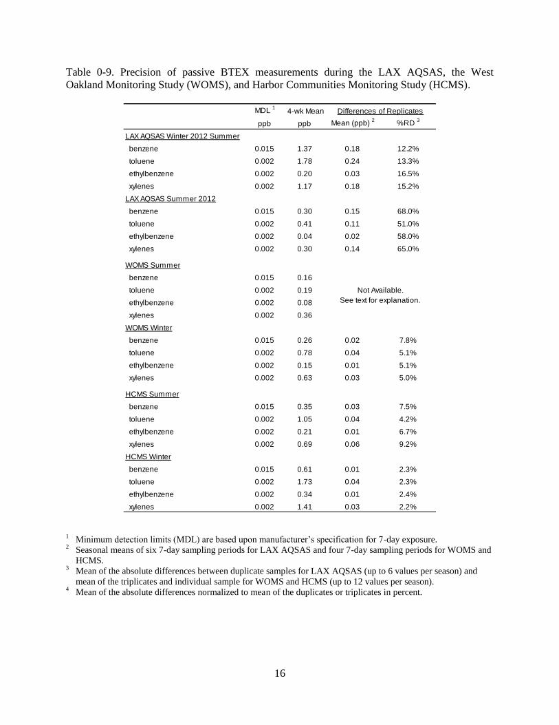
16

Table 0-9. Precision of passive BTEX measurements during the LAX AQSAS, the West

Oakland Monitoring Study (WOMS), and Harbor Communities Monitoring Study (HCMS).

1 Minimum detection limits (MDL) are based upon manufacturer’s specification for 7-day exposure.

2 Seasonal means of six 7-day sampling periods for LAX AQSAS and four 7-day sampling periods for WOMS and

HCMS. 3 Mean of the absolute differences between duplicate samples for LAX AQSAS (up to 6 values per season) and

mean of the triplicates and individual sample for WOMS and HCMS (up to 12 values per season). 4 Mean of the absolute differences normalized to mean of the duplicates or triplicates in percent.

MDL 1

4-wk Mean Differences of Replicates

ppb ppb Mean (ppb) 2

%RD 3

LAX AQSAS Winter 2012 Summer

benzene 0.015 1.37 0.18 12.2%

toluene 0.002 1.78 0.24 13.3%

ethylbenzene 0.002 0.20 0.03 16.5%

xylenes 0.002 1.17 0.18 15.2%

LAX AQSAS Summer 2012

benzene 0.015 0.30 0.15 68.0%

toluene 0.002 0.41 0.11 51.0%

ethylbenzene 0.002 0.04 0.02 58.0%

xylenes 0.002 0.30 0.14 65.0%

WOMS Summer

benzene 0.015 0.16

toluene 0.002 0.19

ethylbenzene 0.002 0.08

xylenes 0.002 0.36

WOMS Winter

benzene 0.015 0.26 0.02 7.8%

toluene 0.002 0.78 0.04 5.1%

ethylbenzene 0.002 0.15 0.01 5.1%

xylenes 0.002 0.63 0.03 5.0%

HCMS Summer

benzene 0.015 0.35 0.03 7.5%

toluene 0.002 1.05 0.04 4.2%

ethylbenzene 0.002 0.21 0.01 6.7%

xylenes 0.002 0.69 0.06 9.2%

HCMS Winter

benzene 0.015 0.61 0.01 2.3%

toluene 0.002 1.73 0.04 2.3%

ethylbenzene 0.002 0.34 0.01 2.4%

xylenes 0.002 1.41 0.03 2.2%

Not Available.

See text for explanation.

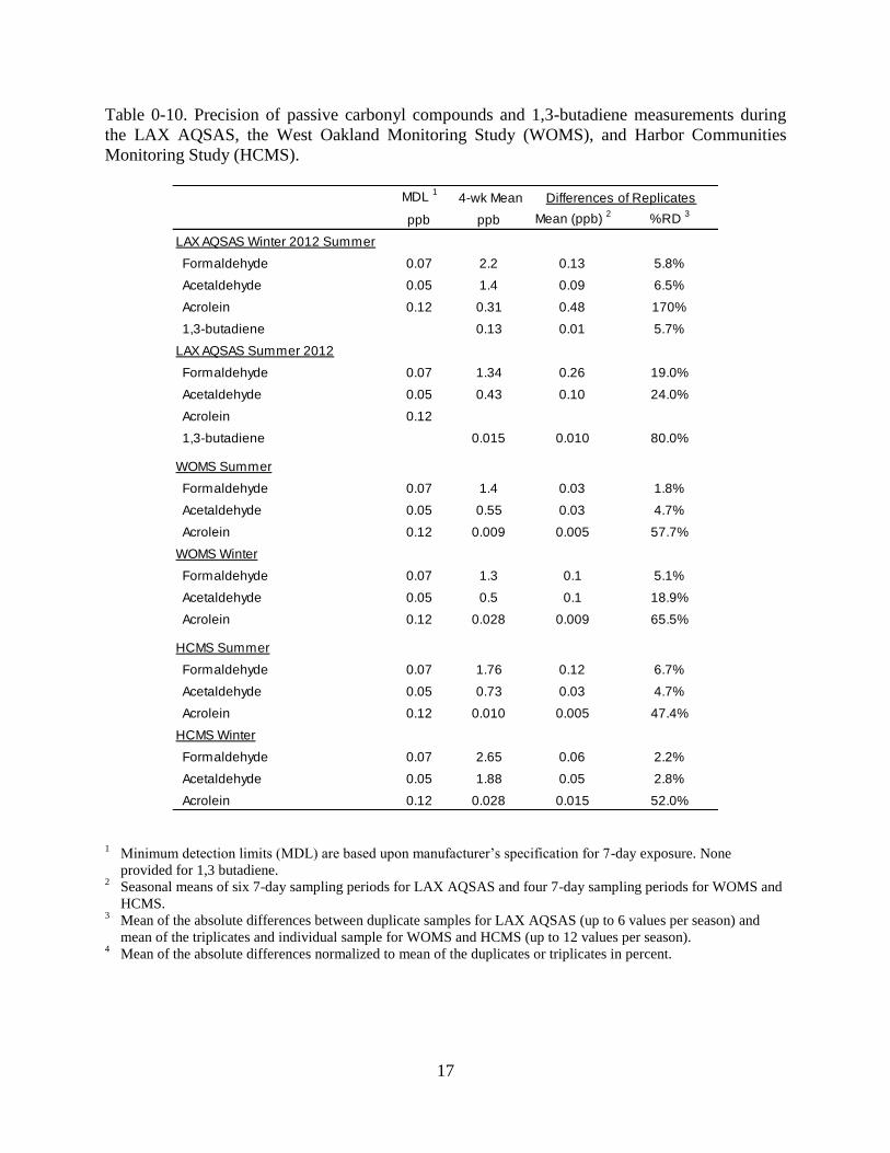
17

Table 0-10. Precision of passive carbonyl compounds and 1,3-butadiene measurements during

the LAX AQSAS, the West Oakland Monitoring Study (WOMS), and Harbor Communities

Monitoring Study (HCMS).

1 Minimum detection limits (MDL) are based upon manufacturer’s specification for 7-day exposure. None

provided for 1,3 butadiene. 2 Seasonal means of six 7-day sampling periods for LAX AQSAS and four 7-day sampling periods for WOMS and

HCMS. 3 Mean of the absolute differences between duplicate samples for LAX AQSAS (up to 6 values per season) and

mean of the triplicates and individual sample for WOMS and HCMS (up to 12 values per season). 4 Mean of the absolute differences normalized to mean of the duplicates or triplicates in percent.

MDL 1

4-wk Mean Differences of Replicates

ppb ppb Mean (ppb) 2

%RD 3

LAX AQSAS Winter 2012 Summer

Formaldehyde 0.07 2.2 0.13 5.8%

Acetaldehyde 0.05 1.4 0.09 6.5%

Acrolein 0.12 0.31 0.48 170%

1,3-butadiene 0.13 0.01 5.7%

LAX AQSAS Summer 2012

Formaldehyde 0.07 1.34 0.26 19.0%

Acetaldehyde 0.05 0.43 0.10 24.0%

Acrolein 0.12

1,3-butadiene 0.015 0.010 80.0%

WOMS Summer

Formaldehyde 0.07 1.4 0.03 1.8%

Acetaldehyde 0.05 0.55 0.03 4.7%

Acrolein 0.12 0.009 0.005 57.7%

WOMS Winter

Formaldehyde 0.07 1.3 0.1 5.1%

Acetaldehyde 0.05 0.5 0.1 18.9%

Acrolein 0.12 0.028 0.009 65.5%

HCMS Summer

Formaldehyde 0.07 1.76 0.12 6.7%

Acetaldehyde 0.05 0.73 0.03 4.7%

Acrolein 0.12 0.010 0.005 47.4%

HCMS Winter

Formaldehyde 0.07 2.65 0.06 2.2%

Acetaldehyde 0.05 1.88 0.05 2.8%

Acrolein 0.12 0.028 0.015 52.0%

18

Time-Integrated PM Speciation Sampling and Analysis

High and Medium-Volume Aerosol Samplers

Due to the low ambient concentrations of many toxic components of airborne particulate

matter, such as trace metals (Ni, Mn, Hg, etc.) and higher-MW PAHs (benzo[a]pyrene,

benz[a]anthracene, chrysene, etc.), it is necessary to concentrate the PM from a large volume of

air onto a filter in order to obtain a sufficient mass of material for accurate speciation analysis.

High-volume samplers such as the EcoTech HiVol 3000 or Tisch TE-PNY1123, which draw

air at approximately 1000 liters/min (lpm) through an 8” x 10” sheet of filter paper in a manner

analogous to a vacuum cleaner, have been in use for many years. Size-selective inlets are

available to remove particles greater than 10 or 2.5 µm aerodynamic diameter. While they can

collect large amounts of particulate matter, they are labor intensive to operate and the large filter

sheets result in substantial background lowering the detection limits and increasing analytical

uncertainty. Medium volume samplers, which collect aerosol onto smaller Teflon or glass fiber

filters (typically 47mm diameter) at flow rates from 16.7 to 113 lpm, depending on the

requirements of the size-selective inlet used, have the advantages that they can be pre-weighed

and loaded into sealed cassettes resulting in much lower analytical background and can be used

in automated sequential sampling systems. Commercially available samplers that meet the

Federal Reference Method requirements for PM2.5 monitoring (operating at 16.7 lpm) include the

Thermo Partisol and BGI PQ-200. Since the acceptance of the beta-attenuation method as an

equivalent method by EPA, sequential FRM PM2.5 samplers are no longer manufactured by

many vendors. At this time only the Thermo 2025i Partisol, which can collect up to 16 filters on

a pre-determined schedule, and the Met One SASS which collects up to 8 sequential samples, are

available. Although the lower sample volumes may be insufficient for analysis of PAH from

typical 24hr duration samples collected with the FRM samplers, the low analytical background

allows laboratory compositing of the filter extracts to achieve good results at the cost of reduced

time-resolution.

Low-Volume Aerosol Samplers

Because suitable passive sampling methods are not available to monitor the

concentrations of aerosol pollutants, portable PM2.5 air samplers are used for particle sampling in

saturation monitoring programs. These monitors consist of an impactor to remove particles

above the cut-point of 1, 2.5 or 10 µm in aerodynamic diameter, a filter holder, pump, 12V

power supply, and programmable control timer. A constant air flow rate of 5 L/min is maintained

during sampling by a flow controller. Particles can be collected on either 47 mm diameter Teflon

filters which can be analyzed gravimetrically for mass and XRF for elements (Na-U), or on pre-

fired quartz filters for quantification of organic and elemental carbon (OC and EC) by

thermal/optical reflectance (TOR) analysis. These systems are lightweight and operate on less

than 100W of AC or 12VDC power, making them much easier to install at temporary sites.

Comparable systems are available from Airmetrics (MiniVol), SKC (DCS), and BGI (Omni-FT).

Due to the low flow rate, sample durations of 7-days or more may be needed to collect sufficient

aerosol for analysis of trace components making them suitable primarily for characterization of

the spatial variation in average pollutant concentrations within a study area.

1

MEASUREMENT APPROACHES AND METHODS TO ACHIEVE

COMMUNITY MONITORING OBJECTIVES

This section provides general recommendations for community-scale air quality

monitoring near refineries. While refineries are the main focus of this report, the methods are

also applicable to other industrial sources with fuel combustion emissions or HAPs in common

with refinery emissions. The recommendations in this section are intended to facilitate further

evaluation and discussion by a panel of monitoring experts gathered from academia, industry, the

community and other governmental agencies. It is anticipated that the BAAQMD will use this

report and the panel’s recommendations to develop regulatory requirements for affected facilities

to conduct community-scale air monitoring to supplement the ambient air quality data from

existing criteria pollutant and air toxics monitoring programs.

The objectives of community-scale monitoring include long-term monitoring to

determine potential chronic and acute health effects as well as short-term monitoring during

major accidental releases of emissions. With the possible exception of SO2, H2S, and

perchloroethylene, most of the other pollutants associated with refinery emissions, such as

benzene and polycyclic aromatic hydrocarbons, are also emitted by motor vehicles and other

combustion sources. Therefore, the monitoring data must also provide means for estimating the

incremental contributions of refinery emissions to the observed ambient pollutant concentrations.

As mentioned in Section 3, there is no single chemical profile that can be used in receptor

modeling of refinery emissions. The source contribution of refinery emissions can be estimated

by combining fence-line monitoring data with measurements of downwind concentration

gradients with appropriate background subtraction. Long-term continuous monitoring at the

boundaries of the refinery can also be used to determine trends in emissions and provide

indications of seasonal or operational-cycle variations in emissions.

Community-Scale Monitoring Options

Each of the community-scale monitoring objectives is associated with appropriate

measurement approaches and methods in Table 0-11. Figure 0-9 shows a conceptual illustration

of a monitoring program for a community (blue rectangle) near a refinery (black rectangle) that

combines three monitoring approaches: A) continuous fence-line monitoring at edge of the

facility closest to community; B) fixed site monitoring within the community at locations closest

and further away from the refinery; and C) saturation monitoring to determine pollutant gradients

around the facility and within the community. Table 0-12 shows the available continuous

monitoring and time-integrated sampling methods and the approximate detection limits for

various pollutants of interest. The acute and chronic RELs set by OEHA are also shown for

comparison. Note that the detection limits shown in the table are only estimates provided for

comparison. Actual performance may vary significantly due to the presence of interfering

pollutants, meteorology, operational conditions, and measurement time scale. Table 0-13 and

Table 0-14 compile typical specifications and costs for the various monitoring methods described

in this report. The information presented are representative values based on individual examples

of each type of monitor, in order to enable comparisons. Actual specifications and costs will vary

by manufacturer, model, and options selected.

2

Table 0-11. Measurement approaches and methods to achieve community monitoring objectives.

Charaterization Surveillence

Acute Effects

Routine Monitoring

Acute Effects

Catastrophic Event

Chronic Effects

Routine Monitoring

Duration of

measurement

program

days to weeks continuous continuous days Minimum of 4 weeks

in 2 season

Time-resolution of

meaurements

minutes hourly hourly varies 7 to 14 days

Measurement

Location

refinery boundary fenceline representative

community sites

Grab samping, mobile

sampling

representative

community sites

Number of

measurement sites

multiple downwind edge 1 to 3 sites multiple Mulitiple

("saturation")

Parameters alkanes, olefins, CO,

NH3, HCHO, SO2, NO2,

benzene, butadiene,

HCHO, NO2, H2S

all determined by event benze, butadiene,

HCHO, NO2, H2S,

metals

Recommended

Methods

SOF, DIAL flux

meaurements

OP photometric, auto-GC

or OP, tape samplers,

met

monitoring van +

canisters, med-vol

PM, OP

passive, low-vol PM

Objective

Community ExposureEmissions

3

Figure 0-9. Conceptual illustration of a monitoring program for a community (blue rectangle)

near a refinery (black rectangle) combining: A) continuous fence-line monitoring; B) fixed site

monitoring; and C) multi-site saturation monitoring.

A. Fence-line Monitoring

B. Fixed Site Continuous Monitoring

C. Saturation Monitoring

1.1

1.2 1.32.1 2.2

3.1

3.2

3.3

4.1 4.2 4.3 4.4

5.1 5.2 5.3

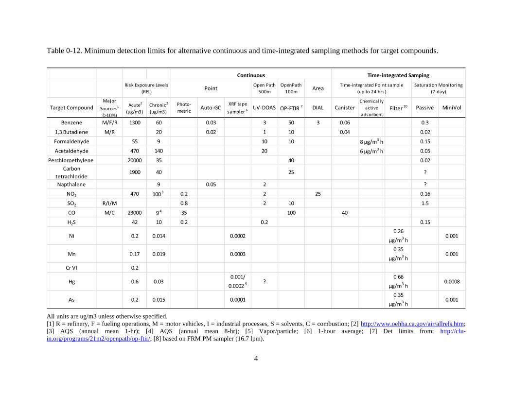
4

Table 0-12. Minimum detection limits for alternative continuous and time-integrated sampling methods for target compounds.

All units are ug/m3 unless otherwise specified.

[1] R = refinery, F = fueling operations, M = motor vehicles, I = industrial processes, S = solvents, C = combustion; [2] http://www.oehha.ca.gov/air/allrels.htm;

[3] AQS (annual mean 1-hr); [4] AQS (annual mean 8-hr); [5] Vapor/particle; [6] 1-hour average; [7] Det limits from: http://clu-

in.org/programs/21m2/openpath/op-ftir/; [8] based on FRM PM sampler (16.7 lpm).

Open Path

500m

OpenPath

100mArea

Target CompoundMajor

Sources1

(>10%)

Acute2

(µg/m3)

Chronic2

(µg/m3) 

Photo-

metricAuto-GC

XRF tape

sampler 6 UV-DOAS OP-FTIR 7 DIAL CanisterChemically

active

adsorbentFilter 10 Passive MiniVol

Benzene M/F/R 1300 60 0.03 3 50 3 0.06 0.3

1,3 Butadiene M/R 20 0.02 1 10 0.04 0.02

Formaldehyde 55 9 10 10 8 µg/m3 h 0.15

Acetaldehyde 470 140 20 6 µg/m3 h 0.05

Perchloroethylene  20000 35 40 0.02

Carbon

tetrachloride1900 40 25 ?

Napthalene 9 0.05 2 ?

NO2 470 100 3  0.2 2 25 0.16

SO2 R/I/M 0.8 2 10 1.5

CO M/C 23000 9 4 35 100 40

H2S 42 10 0.2 0.2 0.15

Ni 0.2 0.014 0.00020.26

µg/m3 h0.001

Mn 0.17 0.019 0.00030.35

µg/m3 h0.001

Cr VI 0.2

Hg 0.6 0.030.001/

0.0002 5?

0.66

µg/m3 h0.0008

As 0.2 0.015 0.00010.35

µg/m3 h0.001

Continuous

PointTime-integrated Point sample

(up to 24 hrs)

Saturation Monitoring

(7-day)

Risk Exposure Levels

(REL)

Time-integrated Samping

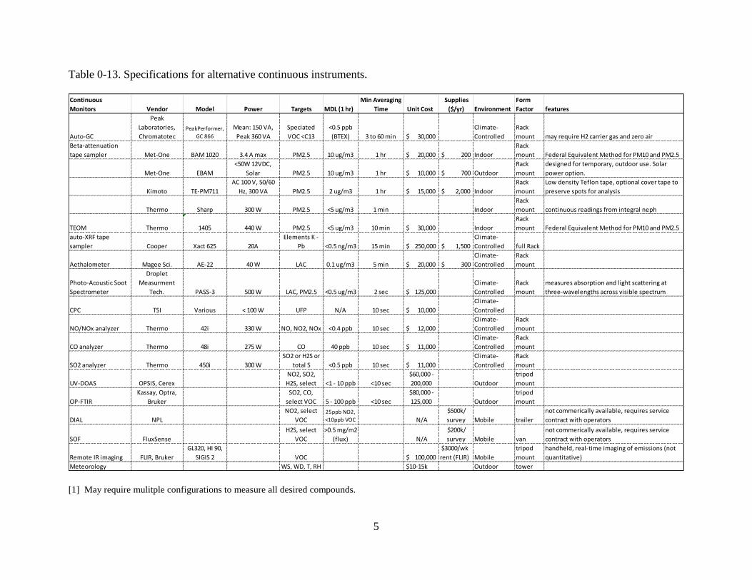
5

Table 0-13. Specifications for alternative continuous instruments.

[1] May require mulitple configurations to measure all desired compounds.

Continuous

Monitors Vendor Model Power Targets MDL (1 hr)

Min Averaging

Time Unit Cost

Supplies

($/yr) Environment

Form

Factor features

Auto-GC

Peak

Laboratories,

ChromatotecPeakPerformer,

GC 866

Mean: 150 VA,

Peak 360 VA

Speciated

VOC <C13

<0.5 ppb

(BTEX) 3 to 60 min $ 30,000

Climate-

Controlled

Rack

mount may require H2 carrier gas and zero air

Beta-attenuation

tape sampler Met-One BAM 1020 3.4 A max PM2.5 10 ug/m3 1 hr $ 20,000 $ 200 Indoor

Rack

mount Federal Equivalent Method for PM10 and PM2.5

Met-One EBAM

<50W 12VDC,

Solar PM2.5 10 ug/m3 1 hr $ 10,000 $ 700 Outdoor

Rack

mount

designed for temporary, outdoor use. Solar

power option.

Kimoto TE-PM711

AC 100 V, 50/60

Hz, 300 VA PM2.5 2 ug/m3 1 hr $ 15,000 $ 2,000 Indoor

Rack

mount

Low density Teflon tape, optional cover tape to

preserve spots for analysis

Thermo Sharp 300 W PM2.5 <5 ug/m3 1 min Indoor

Rack

mount continuous readings from integral neph

TEOM Thermo 1405 440 W PM2.5 <5 ug/m3 10 min $ 30,000 Indoor

Rack

mount Federal Equivalent Method for PM10 and PM2.5

auto-XRF tape

sampler Cooper Xact 625 20A

Elements K -

Pb <0.5 ng/m3 15 min $ 250,000 $ 1,500

Climate-

Controlled full Rack

Aethalometer Magee Sci. AE-22 40 W LAC 0.1 ug/m3 5 min $ 20,000 $ 300

Climate-

Controlled

Rack

mount

Photo-Acoustic Soot

Spectrometer

Droplet

Measurment

Tech. PASS-3 500 W LAC, PM2.5 <0.5 ug/m3 2 sec $ 125,000

Climate-

Controlled

Rack

mount

measures absorption and light scattering at

three-wavelengths across visible spectrum

CPC TSI Various < 100 W UFP N/A 10 sec $ 10,000

Climate-

Controlled

NO/NOx analyzer Thermo 42i 330 W NO, NO2, NOx <0.4 ppb 10 sec $ 12,000

Climate-

Controlled

Rack

mount

CO analyzer Thermo 48i 275 W CO 40 ppb 10 sec $ 11,000

Climate-

Controlled

Rack

mount

SO2 analyzer Thermo 450i 300 W

SO2 or H2S or

total S <0.5 ppb 10 sec $ 11,000

Climate-

Controlled

Rack

mount

UV-DOAS OPSIS, Cerex

NO2, SO2,

H2S, select <1 - 10 ppb <10 sec

$60,000 -

200,000 Outdoor

tripod

mount

OP-FTIR 

Kassay, Optra,

Bruker

SO2, CO,

select VOC 5 - 100 ppb <10 sec

$80,000 -

125,000 Outdoor

tripod

mount

DIAL NPL

NO2, select

VOC25ppb NO2,

<10ppb VOC N/A

$500k/

survey Mobile trailer

not commerically available, requires service

contract with operators

SOF FluxSense

NO2, SO2,

H2S, select

VOC

>0.5 mg/m2

(flux) N/A

$200k/

survey Mobile van

not commerically available, requires service

contract with operators

Remote IR imaging FLIR, Bruker

GL320, HI 90,

SIGIS 2 VOC $ 100,000

$3000/wk

rent (FLIR) Mobile

tripod

mount

handheld, real-time imaging of emissions (not

quantitative)

Meteorology WS, WD, T, RH $10-15k Outdoor tower

6

Table 0-14. Specifications for alternative time-integrated sampling and analysis.

Time-integrated

sample collection Vendor Model Power Targets MDL

Min Averaging

Time Unit Cost

Analysis Cost

($/sample) Environment

Form

Factor features

portable PM2.5 filter

sampler

AirMetrics, SKC,

BGI

MiniVol, DCS,

Omni-FT

12VDC

(rechargable) or

110VAC

PM2.5 mass,

metals < 1 ng/m3 ~7 days $ 5,000 N/A Outdoor

tripod

mount

Portable, battery or solar

operation

FRM PM2.5 filter

sampler

Thermo,

MetOne, BGI

Partisol, SASS,

PQ-200 330 W

PM2.5 mass,

metals,

particulate PAH < 2 ng/m3 24 hrs $8k - 14k

$175 mass &

metals, $180

EC/OC, $800

PAH Outdoor

Stand

Alone

Sequential sampling

models available from

Thermo and MetOne.

filter/XAD sampler EcoTech, Tisch

HiVol 3000, TE-

PNY1123 15A 110VAC

semi-volatile

PAH ~6 hrs $ 4,000 $ 1,000 Outdoor

Stand

Alone

DNPH cartridge

sampler Tisch, Atec TE-423, 8000 2A (5A 12VDC)

acetaldehyde,

formaldehyde >0.5 ug/m3 ~6 hrs $ 13,000 $ 160 Indoor

Rack

mount

Canister sampler Tisch, Xontec TE-323, 901 2A (5A 12VDC) speciated HC <0.1 ppb 1 min $ 10,000 $ 400 Indoor

Rack

mount

Radiello passive

sampler Sigma-Aldrich R141 N/A butadiene <0.02 ppb 24 hrs $ 110 $ 160 Outdoor clip-on

Sigma-Aldrich R145 N/A BTEX <0.02 ppb 24 hrs $ 110 $ 160 Outdoor clip-on

Sigma-Aldrich R165 N/A

acetaldehyde,

formaldehyde >0.1 ppb 24 hrs $ 60 $ 160 Outdoor clip-on

Sigma-Aldrich R170 N/A H2S <1 ppb 24 hrs $ 60 $ 85 Outdoor clip-on

Ogawa passive

sampler Ogawa-USA N/A SO2, NO2 0.5, 0.3 ppb 24 hrs $ 100 $ 100 Outdoor clip-on

1

Fence-line Monitoring

Fence-line monitoring should include continuous open-path monitors (IR and/or UV) that

can detect and record concentrations of major target compounds (e.g., benzene,

perchloroethylene, H2S, SO2) with sufficient sensitivity to identify pollutant fluxes that could

result in exposures above the defined risk levels in the nearby community on an hourly basis or

shorter time scale. Since fence-line monitors only detect pollutant fluxes across a linear path,

they cannot be used to determine the overall emissions from a facility to the community, so

detection limits need not be sufficient to accurately measure long-term ambient concentrations.

More than one type of monitor may be required to provide adequate sensitivity for all target

compounds. Since emissions may originate from various locations within a facility, the

measurement path should be sufficient to cover all likely transport paths between the facility and

community at an appropriate height to be determined by the elevation of the source. Large

separation between sources within a facility or terrain features that interrupt the desired path may

create a need for multiple monitors. Due to the various interferences that can affect open-path

measurements, interpretation of raw data by a trained analyst is essential to avoid false

indications of high emission events. Considering the high capital cost (about $100K per unit),

operating requirements, and limitations of fence-line monitoring, careful consideration should be

given to the level of surveillance required before deploying systems. Detailed evaluation of

routine emissions by remote sensing and study of the distribution of operations within a facility

to determine potential fugitive emissions should precede fence-line monitoring. Toxic metals

cannot be detected by OP methods so, unless a specific point source can be identified, fence-line

monitoring for metals is not recommended. In the case where it is appropriate, and emissions are

of sufficient concern to warrant the high cost ($250K), an XRF filter tape monitor would be the

only available method that could provide continuous surveillance data.

Fixed-Site Monitoring

Due to the difficulties in locating suitable sites and high operating costs, only a very

limited number of fixed monitoring stations can be implemented to monitor the ambient

pollutant concentrations in a community on a long-term basis. Therefore, the location of fixed

monitors must be chosen with care so that they adequately represent the concentrations of

pollutants that community residents are exposed to. Considering that few Bay Area residential

areas exist downwind of refineries during typical weather conditions, the highest exposure to

emissions is likely to occur either near the facility boundaries if the release is near ground level

and atmospheric conditions are stable or at a distance from the facility if emissions are elevated

and there is negative stability. In order to record exposure concentrations during either case, two

fixed monitoring sites are recommended as shown in Figure 4-1; one located in the community

as near the boundary with the facility as possible and another within the more distant half of the

community. The latter requirement may be met by existing BAAQMD monitoring sites in

several communities. Monitoring at fixed sites should include continuous (hourly) measurement

of SO2, H2S, speciated VOC, wind speed and direction at a minimum. Adding NO2, CO, and BC

would be useful for distinguishing between sources of air toxics like benzene. Continuous

monitoring of PM2.5 is likely to have little application for detecting refinery emissions, but

operation of tape samplers would provide potential for analysis of metals by XRF during events.

Cost of implementing fixed site monitoring could range from as low as $30K to add speciated

VOC to an existing SO2 + H2S site up to $150K for a new, fully instrumented monitoring shelter.

2

Daily 24-hr canister and filter samples to be analyzed by GC/MS and XRF should be collected at

these sites for several days during 2 or more seasons. If possible, parallel samples should be

collected at a site without any local source impacts to represent the regional background and

along the fence line monitor path to represent refinery emissions.

Saturation Monitoring

The term “saturation monitoring” is used in reference to ambient air monitoring for the

purpose of establishing more detailed spatial variations in pollutant concentrations at the

community scale. The objectives of this type of monitoring in the context of health risk

assessments is to determine the seasonal or annual average air toxics concentrations at a

sufficient number of locations within the community to: 1) establish the spatial variations in

average concentration of air toxics; 2) identify the potential influence of hotspots of air toxic

emissions on the community’s exposure; and 3) characterize the gradients in air toxic

concentrations from these hotspots. Besides the accuracy, precision, selectivity and sensitivity of

alternative measurement methods, the range of sampling periods, power requirements, size and

portability of sampler or instrument are important consideration in a saturation monitoring study.

To verify the representativeness of the fixed monitoring sites, a one-time saturation

monitoring study should be performed in each community over a period of at least 4 weeks in

both summer and winter. Low-cost, low power or passive samplers can be deployed in a roughly

1 km spaced grid to determine the average spatial pattern of pollutant concentrations. The actual

spacing may need to be varied due to topography, location of local sources, or land use patterns.

If available resources do not permit saturation coverage of the entire community, or if there is no

reason to suspect that significant spatial variations exist within an area, a limited number of sites

can be deployed concentrating on the area nearest the refinery border and the fixed monitoring

sites, as shown in Figure 0-9. Cost of saturation monitoring for SO2, H2S, and speciated VOC

(BTEX, aldehydes, and 1,3-butadiene) is estimated to be about $5000 per site, including

materials, sample analysis and data QA. Extending sampling durations from 7 to 14 days could

reduce costs by almost 50%, but increases the risk of significant data loss if samplers are

damaged or stolen. PM2.5 filter sampling and analysis for mass, elements, and EC/OC would add

about $8000 per site. To reduce costs, low-volume portable filter samplers for metals and OC/EC

can be added to the base configuration of passive SO2, H2S, and speciated VOC at only a subset

of the sites. Considering the monitoring configuration shown in Figure 0-9 as an example, total

cost to determine pollutant gradients in a community would be approximately $90K. Standard

operating procedures for the collection of passive gas samples are provided in Appendix A

(Ogawa samplers) and B (Radiello samplers).

Incident Monitoring

Dispersion modeling

Dispersion modeling can provide valuable insights regarding the transport and range of

impacts of refinery emissions during accidental releases. Using local meteorology (e.g. wind

speed and direction) and details of the emission release (e.g. stack height, temperature and

quantity), the location and magnitude of maximum concentrations can be predicted. Various

release and meteorological scenarios can be simulated to provide predicted pollutant

concentrations and likely areas of impacts. Ambient air quality monitoring may be used to verify

3

these predictions, especially if limit values are predicted to be approached. The modeling results

can be used to make deployment choices for mobile monitoring and collection of grab samples.

Mobile Sampling

The existing BAAQMD monitoring van (described in Appendix C) could provide a

useful tool for characterizing the spatial variations and composition of emissions during

incidents. However, the current instrumentation in the van is designed for detection of mobile

source emissions. Addition of an auto-GC for speciated VOC and a continuous H2S/SO2 monitor

(see Table 0-13) would allow detection of major refinery emissions that could be distinguished

from motor vehicle exhaust, allowing measurements to be made at roadsides and with the on-

board generator operating. During an event the van could be quickly deployed to multiple

locations identified by dispersion modeling as likely to be impacted, where pollutant gradients

could be measured and canister and/or filter samples could be collected for additional speciation.

For rapid deployment it would be necessary to have staff on call that is familiar with the SOPs

for operation of the mobile monitoring system and incident response. When the instruments are

not used for mobile sampling, they can be deployed in various residential and other fixed

locations to complement the saturation monitoring network and the limited number of sites with

supplemental continuous measurements. Examples of recent application of mobile monitoring in

the context of exposure assessment are described in Appendix C along with the applicable

measurement methods.

Another possibility for mobile emergency response is to partner with EPA Region 9’s

Emergency Response Program. This program was developed to respond to environmental

disasters, hazardous materials releases and inland oil spill that threaten human health and/or the

environment. The program is based in San Francisco and includes mobile real-time capabilities

to measure VOC’s, using a number of different technologies such as Area Rae units, H2S,

chlorine, ammonia and hydrogen cyanide. In addition, EPA has particulate matter measurement

capabilities, with some providing real time data. The EPA Emergency Response Program has

well developed sampling protocols in the event that samples need to be collected for further

laboratory analysis. These services are available around the clock and can include a federal on-

scene coordinator that can access additional federal services, if necessary.

Emerging Technology and Cooperative Approaches

The development of new electrochemical and solid-state gas sensors has resulted in a

wide variety of highly portable, low cost monitors that have potential to make large scale

saturation monitoring much more affordable. Gas Sensitive Semiconductor (GSS) technology is

less accurate than traditional methods and more susceptible to bias caused by interferants, but

comes with significant cost savings. Electro-chemical sensors are less prone to interference than

GSS sensors, but can be adversely affected by changes in temperature and humidity. At this time,

none of these methods can provide the sensitivity and accuracy required for regulatory

monitoring of ambient air quality, however, we recommended that their development be

monitored and evaluated over time.

Another novel monitoring approach that bears consideration for the future is to involve

community volunteers for increased spatial coverage during incidents. Some passive sampling

technologies, such as absorbant cartridges and canister grab samples, are easily deployed and

require minimal technical skill to operate, but must be executed in a highly coordinated manner

4

to provide scientifically useful results. If sampling media were distributed in advance to a

network of volunteers within communities that might be impacted by an unplanned chemical

release, existing communication technology such as text message alerts or Tweets could be

employed by BAAQMD or refinery personnel to coordinate sample collection during events.

Once sufficient spatial and temporal data has been collected from the enhanced monitoring

networks proposed in this report, it should be used to evaluate the feasiblility of such a

cooperative incident monitoring plan.

5

REFERENCES

Bay Area Air Quality Management District, 2009. “West Oakland Truck Survey” Available on-

line at http://www.baaqmd.gov/Divisions/Planning-and-Research/CARE-

Program/CARE-Documents.aspx.

California Air Resources Board, 2008. “Diesel Particulate Matter Health Risk Assessment for the

West Oakland Community.” Available on-line at

http://www.arb.ca.gov/ch/communities/ra/westoakland/documents/westoaklandreport.pdf

Campbell D.E.and E.M Fujita (2006). Data Analysis for the Roseville Rail Yard Air Monitoring

Project – First Annual Report. Prepared for the Placer County Air Pollution Control

District Auburn, CA, March 15, 2006

Cuclis, A. (2012). Why Emissions Factors Don’t Work at Refineries and What to do about it.

Presented at the Conference on “Emission Inventories – Meeting the Challenges Posed by

Emerging Global, National, Regional and Local Air Quality Issues”, Tampa, Florida,

August 13-16, 2012.

Dallman, T., Harley, R., and Kirchstetter, T., 2011. Effects of Diesel Particulate Retrofits and

Accelerated Fleet Turnover on Drayage Truck Emission at the Port of Oakland. Environ.

Sci. Technol., 45, 10773-10779.

Fujita, E.M. and D.E. Campbell (2010). West Oakland Monitoring Study. Final report prepared

for the Bay Area Air Quality Management District, San Francisco, CA, October 7, 2010.

Fujita, E.M. and D.E. Campbell (2010). West Oakland Monitoring Study. Final report prepared

for the Bay Area Air Quality Management District, San Francisco, CA, October 7, 2010.

Fujita, E.M., B. Mason, D.E. Campbell and B. Zielinska (2009). Harbor Community Monitoring

Study – Saturation Monitoring. Final report submitted to the California Air Resources

Board, Sacramento, CA, May 15, 2009.

Fujita, E.M., D.E. Campbell, B. Mason, B. Zielinska (2009). Harbor Community Monitoring

Study (HCMS) Saturation Monitoring. Final report submitted to the California Air

Resources Board, Sacramento CA, May 15, 2009.

Fujita, E.M., D.E. Campbell, B. Mason, B. Zielinska (2009). Harbor Community Monitoring

Study (HCMS) Saturation Monitoring. Final report submitted to the California Air

Reesources Board, Sacramento, CA, May 15, 2009.

Fujita, E.M., D.E. Campbell, B. Zielinska, W.P. Arnott, J.C. Chow (2008). Concentrations of

Air Toxics in Motor Vehicle Dominated Microenvironments. Final report submitted to

the Health Effects Institute, HEI contract 4704-RFA03-1/02-16, Boston, MA, January 13,

2008.

6

Fujita, E.M., Zielinska B., Campbell, D.E., Arnott, W.P., Sagebiel, J., Rinehart, L., Chow, J.C.,

Gabele, P.A., Crews, W., Snow, R., Clark, N., Wayne, S., Lawson, D.R., 2007b.

Variations in speciated emissions from spark-ignition and compression ignition motor

vehicles in the California's South Coast Air Basin. J Air Waste Manage Assoc, 57:705-

720.

Kozawa KH, Fruin SA, and Winer AM (2009). Near-road air pollution impacts of goods

movement in communities adjacent to the Ports of Los Angeles and Long Beach.

Atmospheric Environment, 43:2960–2970

Mason, J. Brooks E.M. Fujita, D.E. Campbell and B. Zielinska (2011): Evaluation of Passive

Samplers for Assessment of Community Exposure to Toxic Air Contaminants and

Related Pollutants, Environ. Sci. Technol. 2011, 45, 2243–2249.

Westerdahl D, Fruin S, Fine P, Sioutas C. 2007. The Los Angeles International Airport as a

source of ultrafine particle and other pollutants to nearby communities. Atmos Envir

42:3143-3155.

Westerdahl D, Fruin S, Sax T, Fine P, Sioutas C. 2005. Mobile platform measurements of

ultrafine particles and associated pollutant concentrations on freeways and residential

streets in Los Angeles. Atmos Envir 39:3597-3610.

Zhu, Y.F, Hinds, W.C, Kim, S, Shen, S, Sioutas, C. (2002) Study of ultrafine particles near a

major highway with heavy-duty diesel traffic; Atmospheric Environment, 36, 4323-4335.

A-1

Appendix A

Standard Operating Procedure for Ogawa Passive Monitors

A-2

Equipment List - Ogawa Passive Sampler ID # Description Quantity

1 Sampler Housing 1

2 Sampler Holder 1

3 Mounting Bracket 1

4 Solid Pad 2

5 Pad Retaining Ring 2

6 Stainless Screen 4

7 Diffuser End Cap 2

8 Pre-Coated Collection Pad 2

9 Shelter/Vial 1

10 Sample Bag 1

The Ogawa Pre-Coated Collection Pads come in a few varieties depending on the application.

Specific information on the correct parts for each monitoring application can be found at the

company website (www.ogawausa.com).

A-3

Assembly of the Ogawa Passive Sampler should be completed in a clean, indoor environment

devoid of dust and then transported to the sampling site. Dirt and oils from your skin can affect

the Ogawa Sampler if contact is made with the collection pads so gloves and/or a sterile pair of

tweezers should be used for assembly.

To assemble, remove the Ogawa Sampler Housing from the Sampler Holder and the Opaque

Vial. Remove the Diffuser End Cap from one side of the Sampler Housing and remove the two

stainless screens behind the Diffuser End Cap. The Solid Pad and Pad Retaining Ring should be

visible inside of the sampler and should not be removed. If they come loose, just insert the Solid

Pad into the Sampler Housing first and then slide the Pad Retaining Ring above it to hold it in

place.

The Pre-Coated Collection Pads will come sealed in a vial and a resealable aluminum envelope.

Remove one Collection Pad from the vial with the tweezers and place it in between the two

Stainless Screens. Insert this assembly into the Ssampler Housing taking care that it sits level on

top of the Retaining Ring. The fit should be loose. If it feels snug, then remove and try again.

Then, snap the Diffusion End Cap into place. Repeat this process on the other end of the

Sampler Housing if two measurements are being conducted. See below.

After assembling the Sampler Housing, insert it into the Sampler Holder as shown below. The

assembled sampler should now be sealed into the Sample Bag, removing as much as air as

possible to prevent contamination. Place the bag inside the Opaque Vial with the Mounting

Bracket, screw on the lid, and transport to the sampling site. See Below.

A-4

At the sampling site, remove the Ogawa Sampler from the Opaque Vial and Sample Bag. Attach

the sampler to clothing for personal exposure or to the Mounting Bracket for ambient monitoring

as shown below.

The Mounting Bracket can be easily attached to objects such as fences and poles with zip ties. If

sampling outdoors, the Opaque Vial should be used as a shelter. It can easily be slipped over the

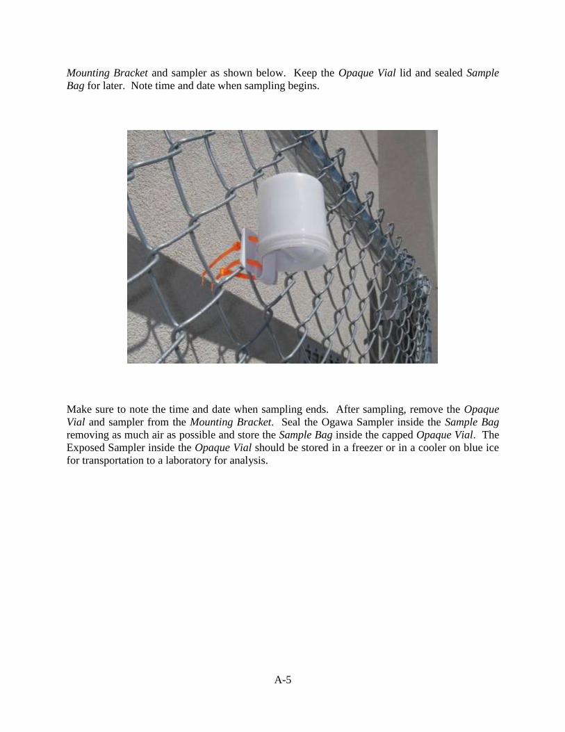
A-5

Mounting Bracket and sampler as shown below. Keep the Opaque Vial lid and sealed Sample

Bag for later. Note time and date when sampling begins.

Make sure to note the time and date when sampling ends. After sampling, remove the Opaque

Vial and sampler from the Mounting Bracket. Seal the Ogawa Sampler inside the Sample Bag

removing as much air as possible and store the Sample Bag inside the capped Opaque Vial. The

Exposed Sampler inside the Opaque Vial should be stored in a freezer or in a cooler on blue ice

for transportation to a laboratory for analysis.

B-1

Appendix B

Standard Operating Procedure for Radiello Passive Monitors

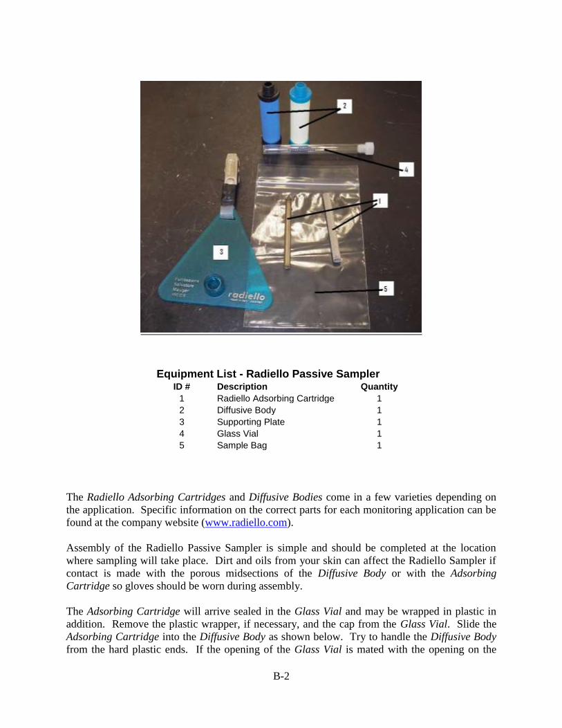
B-2

Equipment List - Radiello Passive Sampler ID # Description Quantity

1 Radiello Adsorbing Cartridge 1

2 Diffusive Body 1

3 Supporting Plate 1

4 Glass Vial 1

5 Sample Bag 1

The Radiello Adsorbing Cartridges and Diffusive Bodies come in a few varieties depending on

the application. Specific information on the correct parts for each monitoring application can be

found at the company website (www.radiello.com).

Assembly of the Radiello Passive Sampler is simple and should be completed at the location

where sampling will take place. Dirt and oils from your skin can affect the Radiello Sampler if

contact is made with the porous midsections of the Diffusive Body or with the Adsorbing

Cartridge so gloves should be worn during assembly.

The Adsorbing Cartridge will arrive sealed in the Glass Vial and may be wrapped in plastic in

addition. Remove the plastic wrapper, if necessary, and the cap from the Glass Vial. Slide the

Adsorbing Cartridge into the Diffusive Body as shown below. Try to handle the Diffusive Body

from the hard plastic ends. If the opening of the Glass Vial is mated with the opening on the

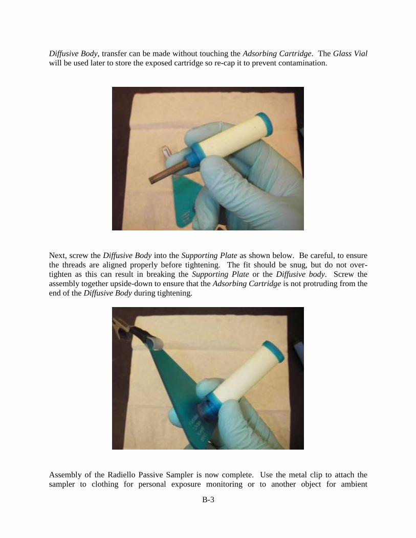
B-3

Diffusive Body, transfer can be made without touching the Adsorbing Cartridge. The Glass Vial

will be used later to store the exposed cartridge so re-cap it to prevent contamination.

Next, screw the Diffusive Body into the Supporting Plate as shown below. Be careful, to ensure

the threads are aligned properly before tightening. The fit should be snug, but do not over-

tighten as this can result in breaking the Supporting Plate or the Diffusive body. Screw the

assembly together upside-down to ensure that the Adsorbing Cartridge is not protruding from the

end of the Diffusive Body during tightening.

Assembly of the Radiello Passive Sampler is now complete. Use the metal clip to attach the

sampler to clothing for personal exposure monitoring or to another object for ambient

B-4

monitoring. If monitoring is being done outside where the sampler may be exposed to rain, care

must be taken to attach the sampler under an overhanging feature. Plastic shelters can be

fashioned easily from disposable cups or other containers but make sure not to inhibit airflow

from reaching the sampler. Note start time and date. See below.

After exposure, note end time and date. Sampler should be taken down by unscrewing the

Diffusive Body from the Supporting Plate. Slide exposed Adsorbing Cartridge back into Glass

Vial by mating the two openings. Recap the Glass Vial containing the Adsorbing Cartridge and

seal it into the Sample Bag. Remove as much air as possible from the Sample Bag to prevent

contamination. Place the Sample Bag into a freezer or cooler containing blue ice for

transportation to a laboratory for analysis.

C-1

Appendix C

Operating procedures for BAAQMD mobile monitoring system

C-2

This document describes basic setup and operating procedures for the mobile air quality

monitoring system used in the West Oakland Monitoring Study (WOMS) in 2009-2010. The

instrument platform is a 2008 Ford E-350 cargo van with raised roof and rear air conditioning

modified by E-N-G Mobile Systems, Inc. to include an instrument rack, desk/workbench,

calibration gas cylinder rack, and 120VAC and 12VDC power system that can operate off of on-

board batteries or line power. The following instruments/measurements are included in the

standard setup:

Instrument Parameters measured

2Btech model 400 NO

2Btech model 202 O3

TEI model 48 CO

ppbRAE 3000 VOC

LiCor CO2

DRI mini-photoacoustic BC

TSI model 3007 CPC Ultrafine particle conc.

TSI DustTrak II model 8530 PM

Garmin GPS-16 Lat, long, elevation, speed, direction

Davis Weather Envoy T, RH, wind speed, direction

All instruments listed are capable of making real-time measurements of the listed parameters

with averaging times as low as 10 seconds.

Ambient air is drawn into the van via an electric fan-driven roof duct into glass or stainless-steel

plenum for connecting gas and particle sampling instruments, respectively. The air velocity in

the duct can be adjusted via the fan control to minimize anisokinetic sampling effects when

making aerosol pollutant measurements while the van is in motion, or if there is a significant

cross-wind at a stationary sampling location.

An Environics 6100 gas-diluter/ozone generator connected to cylinders of zero air and a span gas

mixture is also included to allow frequent checks of the accuracy of the gaseous pollutant

monitors.

C-3

Air inlet manifold

There are four ¼” stainless-steel tubes exiting the inlet duct that can be connected to particle

sampling instruments via flexible conductive tubing. The connection tubes are curved to avoid

impaction losses, and sharp bends in the conductive tubing should be avoided. A ¼” Teflon hose

also exits the fan duct and connects to a particle filter cartridge that is followed by a glass

plenum with up to 4 connection ports for gaseous pollutant sampling. The output of the gas

calibrator should also be attached to this plenum. If additional connections are required it is

permissible to install “T” connectors in the lines downstream of the plenum for gas sampling.

Before the start of monitoring each day, check that there are no open ports on either the glass or

stainless steel inlet manifolds. Turn on the fan in the inlet duct and adjust to an appropriate

setting (12VDC breaker on wall panel must be on). The fan speed should be set to produce air

velocity at the intake on the roof that is near the median value of the anticipated ambient wind

speed and/or van travel speed. An assistant with a handheld anemometer is recommended for

making this adjustment.

Photos of the inlet duct and fan control, stainless steel plenum exiting duct, and glass plenum with particle filter (replaceable paper disk filter is in the orange cartridge).

C-4

On-board power system

The on-board power systems are operated from the control panel located on the wall behind the

driver’s seat:

When operating the equipment with the van connected to an external AC line (aka “shore

power”), the toggle switches in the upper left section should be in the ON position, as shown

above. If starting up without shore power, flip on AC Circuit switches for inverter, instrument

rack, and utility outlets after starting the inverter, as described below.

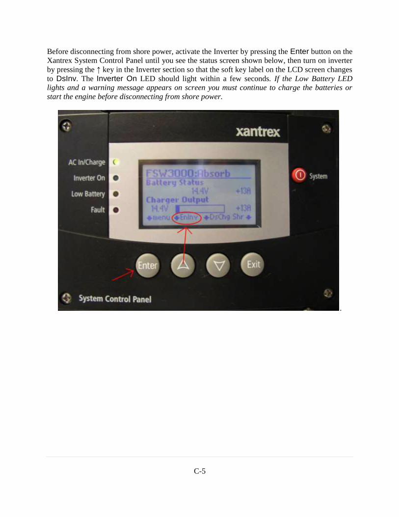
C-5

Before disconnecting from shore power, activate the Inverter by pressing the Enter button on the

Xantrex System Control Panel until you see the status screen shown below, then turn on inverter

by pressing the ↑ key in the Inverter section so that the soft key label on the LCD screen changes

to DsInv. The Inverter On LED should light within a few seconds. If the Low Battery LED

lights and a warning message appears on screen you must continue to charge the batteries or

start the engine before disconnecting from shore power.

.

C-6

INSTRUMENTS

2Btech model 400 Nitric Oxide monitor

Connections:

12VDC power supply must be connected to jack on rear panel of instrument and plugged into

110V power strip on rack.

9-pin RS232 serial cable connected from instrument rear panel to USB port on notebook PC via

a serial-USB converter.

¼” Teflon tubing from inlet on rear panel to glass manifold.

Startup:

Press power switch on front panel.

Wait 20 minutes for warm-up cycle to complete, after which display will show NO concentration

alternating with flow and ozone supply readings. If logging data to computer the internal

datalogging must not be enabled and the averaging time should be set to 10 seconds (default).

Otherwise, see instrument manual (pdf file on PC) for internal datalogging and downloading

instructions.

2Btech model 202 Ozone monitor

Connections:

12VDC power supply must be connected to jack on rear panel of instrument and plugged into

110V power strip on rack.

9-pin RS232 serial cable connected from rear panel to PC docking station (Com1).

¼” Teflon tubing from inlet on rear panel to glass manifold.

Three voltage inputs for logging analog data output by other instruments are available on the rear

of the ozone monitor. Voltages received through these jacks will be recorded and/or transmitted

along with ozone concentrations if the ozone monitor is operating.

Startup:

Press power switch on front panel.

If logging data to computer the internal datalogging must not be enabled and the averaging time

should be set to 10 seconds (default). Otherwise, see instrument manual (pdf file on PC) for

internal datalogging and downloading instructions.

DRI mini-photoacoustic (PA)

Connections:

Universal power cord to 110V outlet.

Conductive tubing (black plastic) from inlet on rear panel to one of the stainless steel manifold

tubes exiting from the duct on ceiling.

Flexible mesh-wall tubing from outlet (rear panel) to vacuum pump inlet using quick

disconnects.

USB hub connected to front panel USB port.

C-7

USB cable to keyboard/touchpad combo or mouse.

Wireless monitor transmitter connected to USB hub. Wireless monitor must be connected to

12VDC power outlet and to receiver via serial cable. Receiver power supply plugged into 110V

outlet.

Startup:

Power switch on rear of case On.

Turn computer on by pressing button on front panel (right of monitor). Blue LED will light.

Switch on vacuum pump.

Monitors have power button below screen (should be left on).

LabView application should start up automatically. If not, see PA documentation.

Allow to warm up for at least 30 minutes. Check laser power graph on Diagnostic tab to verify

stability before starting data collection.

Once all instruments have completed warmup cycles, go to the “O3 and NO tab” and enable data

logging for these instruments. Current values should appear within 10 seconds. Warning:

enabling serial data logging when no data is being transmitted by the instruments may cause the

program to freeze up.

Initial screen view of photoacoustic instrument LabView program

C-8

.

Diagnostics tab of photoacoustic instrument LabView program. Top graph shows laser power

during warmup (not stabilized yet).

Other tabs are included for simultaneous recording of data from other samplers, but are not

needed if data is logged to the notebook PC (recommended).

ppbRAE 3000 VOC monitor

connections:

¼” Teflon tubing from inlet probe to glass manifold

For run times greater than 8 hrs, connect 12VDC battery charger to the instrument cradle and

plug into 110V outlet. Otherwise, charge the instrument overnight.

USB device cable from jack on left side to USB port on laptop (for downloading stored data).

startup:

press center yellow button and hold until beep. Verify that data is logging (floppy disc icon at

bottom of display. Allow 1 minute for warm-up.

C-9

DustTrak II aerosol monitor

connections:

Conductive tubing (black plastic) from inlet on rear panel to one of the stainless steel manifold

tubes exiting from the duct on ceiling.

For run times greater than 12 hrs, connect 12VDC battery charger to the instrument cradle and

plug into 110V outlet. Otherwise, charge the instrument overnight.

(IMPORTANT: the battery only charges while unit is turned on).

USB device cable from jack on left side to USB port on laptop (for downloading stored data).

startup:

press On button above display.

When ready, touch Start on screen. Should start logging data within 1 minute. No warmup

needed.

TSI 3007 CPC

connections:

¼” Teflon tubing from inlet to glass manifold.

6VDC power supply, coaxial jack next to inlet.

USB serial cable to laptop for data acquisition.

startup:

Replace the alcohol cartridge with a freshly charged one, if necessary. Cartridges must be

refreshed after 5-6 hours of operation.

Press black button to start 10 minute warmup cycle. Warmup can be skipped by pressing the

enter key.

Start TSI Aerosol Instrument manager software on laptop. Open new file of type for 3007. When

instrument is recognized, press Start to begin data logging.

The logging interval can be adjusted via the Log Mode 1 tab of the dialog box accessed from the

Run/Properties menu item. Make sure the number of samples is set to a large enough value to

accommodate the logging interval and run time you wish to use. Com port assignment and the

Instrument Clock can also be changed via the Properties menu.

TEI CO monitor

Connections:

Universal power cable to 110V power strip on back of rack.

Analog output cable to analog input B (stereo mini-plug jack) on back of 2Btech Ozone monitor

(data is logged along with ozone data).

¼” Teflon tubing from inlet probe to glass manifold.

Startup:

Press start button on front panel.

C-10

Allow to warm up for about 30 minutes prior to data collection. Check rotameter on front panel

for stable flow rate (about 0.7 lpm).

If necessary, press Run button until indicator lights under Zero and Span on display are off.

TEI CO analyzer front panel with light indicating instrument is in Span mode circled – this

indicator should be off when collecting data.

GPS

Check that GPS USB cable is attached to laptop. Start ‘Spanner’ program from desktop icon. It

should indicate that a Garmin GPS-18 is recognized. If not, try reconnecting USB cable, and/or

rebooting. Once Spanner is running, data may be logged via various applications that read

NMEA standard data streams. A Hyperterm shortcut named ‘Garmin GPS.ht’ on desktop can be

used to view the raw data and verify the Com port number.

PC data logger

Serial data streams from the 2Btech NO and ozone monitors can be logged along with GPS data

on the notebook PC using the DAQfactory application. Data are logged as running 10 second

averages to an Excel readable file stored in the C:\data folder. The program automatically creates

a file with the name DAQraw_yymmdd.xls and continuously appends data to that file whenever

data logging is enabled.

To begin logging data:

1. if GPS data is desired, first run the Spanner application from the desktop icon.

2. run DAQfactory from the desktop icon labeled “datalogger”.

3. verify that current values from all operating instruments are displayed in the application

window and the UTC time from the GPS is advancing (PM data are indicated on the

C-11

application front panel, but at present the continuous data output features of the

DustTrak are not available due to a design flaw)

a. if serial data from the ozone monitor are not being received via Com port 1, you

may need to reboot the PC after confirming that the ozone monitor is operating

and properly connected.

4. the application should immediately begin logging data. You can suspend logging by

clicking on the button labeled “Datalogging ON/OFF”. Current values will still be

displayed while datalogging is suspended.

5. it is recommended that you periodically check to confirm that current values for all

operating instruments are displayed by the application.

If additional instruments are connected or data cable connections are changed it may be

necessary to update the comm. port assignments using the ‘Quick’ menu ‘Device Configuration’

feature of the application (see documentation for details).

Meteorology Package

If met data is desired during operation, the wireless sensor package should be deployed to a

suitable location. Plug in the power supply for the met station console/receiver. Confirm

communication with the sensor package by moving the wind vane and observing the wind rose

on the display. The sensor package should then be mounted on the tripod with the arm of the

anemometer pointing due North. Data from the station can be downloaded and/or viewed in real

time by connecting the console to a USB port on the laptop and running the WeatherLink

software (if installed).

Wireless met station console.

C-12

Synchronizing clocks:

Should be done before the start of data collection each day if 10 second average data is being

collected. For longer averages, weekly synchronization may be adequate.

Adjust Windows system time on notebook PC to current time (GPS or cell phone are good

reference time sources). This system time will be recorded with each data point by the

datalogging software.

Adjust Windows system time on PA computer to match laptop (you can do this while the

LabView program is running, but it may result in duplicate time signatures in the data logs if you

adjust to an earlier time). This will sync all data being logged together (BC, NO, O3, and CO).

For DustTrak, set time via the Setup menu, which is only accessible when sampling is stopped.

For CPC, sync internal clock to laptop when starting AIM software

For ppbRAE, press N/- twice to see system time and date. If needed, sync internal clock by

accessing the instrument configuration using ProRAE Suite software on the laptop (see data

retrieval instructions).

Data Retrieval

The ppbRAE 3000 does not allow real-time data acquisition, so data from the internal logs must

be downloaded. To download:

1. start the ProRAE Suite software on the laptop

2. press the N/- button on the instrument repeatedly until the “Enter PC comm” message

appears, then press Y/+

3. select “Receive Data” from software menu and follow prompts

4. to backup data files to laptop, select a test data set on screen and use the “Options\export”

menu item.

DustTrak internal data logs can be retrieved using TSI TrakPro software on the laptop. Stop the

instrument (but don’t turn off), then start the program. The software should detect the instrument

if it is connected to a USB port. Click the Retrieve Data button on the toolbar and follow

instructions to download. Data can be backed up to Excel-readable files via the File/Export menu

item.

PA data files can be copied from the C:\BCdata directory on the PA computer. This can be done

while the LabView program is running or stopped. Two text files in a date-named folder are

created each day. One contains complete ‘raw’ data (recorded about every 2 seconds) with lots of

diagnostics, and the other contains 1 minute averages and selected BC diagnostics.

C-13

Shut down

At the end of data collection:

Switch off the pump for the PA. Stop the PA LabView program by clicking on the green On/Off

switch on the left side of the application window. The program should stop after a few seconds.

The computer can be shut down via the normal Windows method after data is copied.

Stop the data acquisition program on the PC.

Click the stop button of the AIM application on the laptop to cease acquiring CPC data.

After downloading data, press and hold the center yellow button on the ppbRAE for 5 extremely

loud beeps until shutdown occurs.

Press the Stop button on the DustTrak screen. Power off by pressing the button above the screen

(this will prevent battery charging and data retrieval).

Press the black power button on the CPC to shut down. If the instrument will not be used again

that day, remove the alcohol cartridge and place it in a recharging tube. Plug the instrument

chamber with the cap from the tube.

The 2Btech instruments and TEI CO can be switched off at any time, but if a span check or

calibration is planned it may be advisable to leave them running to avoid additional warm-up

time.

After backing up all data, close all applications on the laptop and shut down.

Turn off all AC and DC circuits, except Shore Power, via switches on left side of control panel.

If system will be used again soon: Connect van to shore power, if available. Switch the inverter

Off from the System Control Panel (press DsInv button). Check that the green AC In/Charge

LED is lit (if not. press the EnChg button).

If system will not be used for an extended period: Switch off inverter on control panel. Check

battery voltage on display. If fully charged (>12 V), turn off charger with DsChg button on

control panel. Otherwise, allow to charge (deep-cycle batteries may be damaged is left in a

discharged state for extended periods).

Calibration checks

Periodic zero and span checks are required to ensure the accuracy of the measurements. If time

permits, checks should be done prior to and immediately after each period of data collection.

NO and CO can be checked using compressed zero air and a certified gas standard. A gas

dilution system like the Environics 6100 will produce known concentrations of the target gases at

C-14

concentrations ranging from zero to the upper limit of the range of anticipated ambient

concentrations (i.e., the span value). See the manufacturer’s instructions for the required line

pressures and calculation of dilution settings. If the gas mixer is already set-up with zero air and

span gas blend, the procedure is as follows:

- warm up calibrator for at least 30 minutes

- open cylinder valves and adjust pressure to approx. 25 psi.

- select concentration mode (press button under CONC on screen)

- if desired gas is not displayed, press GAS to display a list, move cursor, then press

SELECT.

- enter desired span gas and/or ozone concentration and total flow rate (should be

greater than combined flow to all running instruments)

- press START

- if using a gas blend, press VIEW to see concentrations of all components

- when instrument readings have stabilized (may take several minutes), record if

additional span concentrations are desired, press EDIT, change values, then UPDATE

- when finished, press STOP and close all gas cylinder valves.

With all instruments fully warmed up, zero air should be introduced to the glass inlet manifold at

a flow rate in excess of the total intake flows of all instruments connected to the manifold. Wait

until readings appear to be stable4 and record the average value over a period of 5 minutes. If the

average reading differs significantly from zero, adjust the offset value via the instrument’s setup

menu (see manual). Once the zero has been checked and adjusted, introduce gas at the span value

concentration and record the average5. If desired, the displayed span readings may be adjusted,

however significant variations generally indicate some sort of malfunction.

The zero value of the ppbRAE 3000 VOC monitor may also be checked and adjusted during this

process. An automated zero adjustment can be made via the setup menu. For maximum low end

sensitivity, zeroing with an activated carbon filter tube on the inlet is recommended (see manual

for instructions). Span adjustment is also possible, but is of limited value since the response of

the PID varies substantially with organic pollutant composition.

The zero reading of the DustTrak aerosol monitor should be checked by attaching a particle filter

to the inlet, recording the low reading, then running the automated zeroing cycle. The

photoacoustic instrument automatically adjusts the zero value at regular intervals during data

collection, but an occasional check with a particle filter on the inlet is still recommended. An

inlet filter should also be connected to the CPC periodically, and the reading noted if it is greater

than zero. Generation of known concentrations of aerosol particles is beyond the scope of field

operations, so no span checks are possible.

4 Since the NO monitor measures the difference in ozone concentration before and after titration

by ambient NO, the readings at concentrations below 20 ppb are subject to a relatively large

amount of electronic noise making them very unstable. 5 Application of extremely low humidity (compressed) air to the 2BTech NO monitor will result in erroneous

readings. Span gas should be humidified using a 24” length of Naphion tubing attached to the inlet during

calibration checks.

C-15

Maintenance

Inlet filters are used on all gas monitors to remove moisture and particles from the incoming air.

This is particularly important for the NO monitor. The line filter installed between the ceiling

duct and the glass manifold should be inspected periodically and the replaced if dirty or clogged.

The frequency will depend on the concentration and nature of aerosols as well as ambient

humidity. Operating in extremely dusty conditions such as on unpaved roads or in areas with

high concentrations of combustion aerosols will require more frequent filter changes.

The ppbRAE and DustTrak have internal filters that should be checked and replaced

periodically. See the manuals for details.

Although the concentrations reported by the continuous monitoring instruments are not a

function of the air flow rate, the inlet flows should be checked periodically with a reference

meter to assure that they are within the specified range. Significant variations in flow rate are

usually symptomatic of internal leaks or pump failure. The entire inlet system should also be

checked for leaks by comparing the total flow at the inlet manifold to the sum of the individual

instrument flows.

Although all instruments can be operated on line power, it may be desirable at times to reduce

power use by running on internal batteries. The batteries also provide backup in the event of a

power outage. The DustTrak and ppbRAE have rechargeable internal batteries, but the CPC and

weather station use replaceable alkaline or externally rechargeable NIMH batteries.

AIR MONITORING TECHNOLOGY &

METHODOLOGY EXPERT PANEL

REPORT & FINDINGS

Convened by

Bay Area Air Quality Management District July 11, 2013

Page 1

Acknowledgements –

The Bay Area Air Quality Management District (Air District) wishes to thank both Eric Fujita and David Campbell of the Desert Research Institute (DRI) for their work compiling the Review of Current Air Monitoring Capabilities near Refineries in the San Francisco Bay Area. In addition, the Air District wishes to thank members of the Expert Panel listed below for their efforts and time providing input towards the goal of enhancing monitoring efforts at and near Bay Area refineries.

George Allen –Senior Scientist at Northeast States for Coordinated Air Use Management

(NESCAUM)

Michael Benjamin, Ph.D. –Chief of the Monitoring and Laboratory Division at the

California Air Resources Board (CARB)

Kenneth Stroud (Serving for Dr. Michael Benjamin) –Chief of the Air Quality Surveillance

Branch at CARB

Philip Fine, Ph.D. - Assistant Deputy Executive Officer for Science & Technology

Advancement at the South Coast Air Quality Management District (SCAQMD)

Andrea Polidori Ph.D. (Serving for Dr. Fine) - Quality Assurance Manager for Science &

Technology Advancement at the SCAQMD

Jay Gunkelman – Member of the public and fence line monitoring expert

Robert Harley, Ph.D. –Professor in the Department of Civil and Environmental

Engineering at the University of California, Berkeley

Thomas Kirchstetter, Ph.D. - Staff Scientist in the Environmental Energy Technologies

Division at Lawrence Berkeley National Laboratory and an Adjunct Professor in the Civil

and Environmental Engineering Department at the University of California, Berkeley

Denny Larson – Executive Director, Global Community Monitor

Gary Mueller –Principal Air Quality Consultant with the HSE Services, Environmental

Sciences Department of Shell Global Solutions (US) Inc.

Jay Turner, Ph.D. - Associate Professor of Energy, Environmental and Chemical

Engineering at Washington University in St. Louis

Gwen Yoshimura –Air Monitoring Lead in the Air Quality Analysis Office with the

Environmental Protection Agency (EPA), Region 9

Page 2

Executive Summary

The Bay Area Air Quality Management District (Air District) contracted with the Desert Research Institute (DRI) to compile a report that provided a background on current air monitoring capabilities near Bay Area refineries and assembled a panel of air monitoring experts from around the country to review and comment on the DRI report. The Panel agreed that the report adequately addressed the issues and complexity involved with monitoring air quality around Bay Area refineries, in general. They also agreed that the report provided a good starting point for developing further guidance. However, the Panel noted that the report did not include the operating and maintenance costs for each monitoring option and should simply be used to compare and evaluate each monitoring option. In addition, the report could not include every available and applicable monitoring technology but was intended to be a starting point for discussion of options and as a way to evaluate options. Finally, the scope of the report did not allow for a complete discussion of meteorological measurement or other methodologies that might be utilized to estimate exposures.

The Panel generally agreed that an approach that utilized a combination of fence line, community, and mobile monitoring would be required to adequately define exposures during normal operations and when upsets and incidents occur. The fence line monitoring would be leveraged primarily to identify non-routine emissions during normal operation, while the community monitoring would be utilized to develop spatial gradients of chronic exposures. Mobile monitoring would be used to supplement on-going monitoring during major upsets and incidents and to help develop information on spatial variability.

The Panel also recommended that compounds of interest should be identified based on the monitoring goals with relationships and correlations between compounds of interest developed to minimize costs. While it was recognized that not all compounds of interest need to be measured, volatile organic compounds (VOC) should be the primary, initial focus.

Panel members generally agreed that information should be provided to the community through a well-designed website that provides appropriate context and allows more sophisticated users to access more complex and complete data. However, alternate methodologies should also be developed to inform members of the public who lack computer access or need additional information. In addition, a means for the public to provide their observations and experiences should be included and that they should be informed of actions taken in response to observations to build trust.

Data quality and time resolution were major topics of discussion, with Panel members again suggesting that different approaches be utilized for different monitoring goals. For example, fence line monitoring should employ higher time resolution than community monitoring, but

Page 3

community monitoring time resolutions should be increased during upsets and incidents when acute exposures are of concern.

Since technologies are rapidly evolving, the Panel recommended that regular review of available instrumentation should occur with a methodology to cost-effectively update the in-place network. Lines of open and honest communication should be established between industry, the community and regulators to ensure appropriate value is provided by the developed network.

Page 4

Background

On August 6, 2012, a substantial fire occurred due to a hydrocarbon leak at a crude oil processing unit at the Chevron Refinery in Richmond, CA. The fire resulted in a large plume of black smoke and visible emissions from a refinery flare. The Contra Costa County Health Department issued a community warning and ordered a shelter-in-place for about five hours in Richmond, San Pablo and North Richmond. Thousands of residents sought medical treatment, with most suffering respiratory and/or eye discomfort.

The August 6, 2012 incident prompted the Bay Area Air Quality Management District (Air District) staff and Board of Directors to identify a series of follow-up actions to enhance the Air District’s response to similar incidents (Board of Directors, October 17, 2012). One of these actions was to convene a panel of air monitoring experts (Expert Panel) to recommend technologies, methodologies and tools to enhance community air monitoring capabilities near refineries. Another related follow-up action was the development of a new Air District Petroleum Refining Emissions Tracking rule, which would include a requirement that Bay Area refineries establish and operate fence line and community air monitoring systems consistent with guidelines to be developed by the Air District.

As part of this effort, the Air District contracted with Desert Research Institute (DRI) to compile a report that provides background on current air monitoring capabilities near Bay Area refineries and potential air monitoring technologies, methodologies and tools to:

Provide air quality information for communities near refineries

Gather data to evaluate health impacts associated with air quality near refineries

Track air quality changes and trends over time near refineries

The DRI report reviewed and evaluated measurement approaches and methods for assessing the impacts of refinery emissions on ambient concentrations of criteria and air toxics pollutants in nearby communities. Available data for refinery emissions along with ambient air concentrations were reviewed and compared to established levels for acute and chronic health effects to identify the species that should be considered for air monitoring. Various monitoring options were then associated with the following monitoring objectives: short-term characterization of emission fluxes; long-term continuous fence-line monitoring of plant emission releases to the community; community-scale monitoring with varying time scales to evaluate potential chronic or acute health impacts; and episodic monitoring during upsets and incidents. These objectives were reconciled with available air quality data from existing Air District criteria and air toxics pollutant monitoring programs, and air monitoring (both regulatory and voluntary) by the refineries to identify existing gaps in information or useful supplemental data. Published results from relevant applications of the monitoring approaches were reviewed and the specifications for selectivity, sensitivity, precision, accuracy and costs of

Page 5

commercially-available continuous or semi-continuous monitors, and time-integrated sampling and analysis methods were compared for each target pollutant to determine the positive and negative attributes of each monitoring approach and method. Potential augmentations to existing monitoring in the Bay Area were suggested with scalable options. It was the intent of the Air District to utilize the DRI report to provide the Panel with a starting point of discussion.

Page 6

DRI Report

The DRI report, Review of Current Air Monitoring Capabilities near Refineries in the San Francisco Bay Area (October 29, 2013 Revision), was designed to provide the expert panel with a starting point for discussion by:

Evaluating current air monitoring capabilities

Developing a matrix of additional technologies, methodologies and tools that could be

employed to enhance air monitoring capabilities and provide information about

emissions from refineries

Providing costs associated with the technologies, methodologies and tools

Outlining the potential advantages and disadvantages of each option

Providing a short description of the process used and how the matrix was developed

The DRI report is available at: http://www.baaqmd.gov/~/media/Files/Technical%20Services/DRI_Final_Report_061113.ashx

DRI Report Executive Summary

The DRI report provided historical and emissions information from the five Bay Area refineries, which includes Chevron in Richmond, Shell in Martinez, Tesoro in Martinez, Valero in Benicia and Phillips 66 in Rodeo. The refineries account for approximately half of the PM2.5, reactive organic gases (ROG) and NOx and over 90% of the SO2 from stationary sources in the Bay Area. In addition, the report also provided a review of available toxic air contaminant (TAC) information and health risk assessment information and findings. This information could be used to help develop a list of compounds of interest and appropriate sampling methodologies that could be employed near the refineries.

DRI provided a review of current Air District and facility monitoring throughout the Bay Area to determine if and where enhancements could be made. This evaluation included meteorological, individual compound, and special study data as well as incident response capabilities. While DRI concluded that Air District monitoring sites adequately represent pollutant concentrations throughout the Bay Area in general and within approximately a mile or two of the refineries, in particular, they may not be representative of concentrations near fence lines and during upsets when localized conditions and short duration events may not be adequately captured.

Current commercially available instrumentation was investigated and information and options provided. The instrumentation fell into four major categories:

Page 7

Emissions flux measurements that attempt to determine actual emissions rates from

facilities

Optical remote sensing that uses a light source to measure compounds that pass

through a light beam and that can be used to determine compound concentrations

across a distance

Saturation monitoring that uses many sampling devices that are usually exposed for

longer periods of time to determine more detailed spatial variations in specific

compound concentrations

Continuous monitoring that uses a less instrument “dense” network than saturation

monitoring to provide better time resolved information.

The report then provides information on commercially available measurement technologies that fall into these general categories. In addition, it provides examples of individual equipment and methodologies that could be utilized. The report also covers potential measurement technologies and methodologies that could be effectively utilized during short duration upsets and incidents.

The report’s appendices provide operating procedures that could be utilized to perform saturation monitoring and mobile monitoring that could be employed during short duration events and to help determine spatial variability.

Page 8

Page 9

The Expert Panel Members

George Allen – George Allen is a Senior Scientist at NESCAUM (Northeast States for Coordinated Air Use Management), an interagency association of the eight Northeastern States. He received a B.S. in Electrical Engineering from Tufts University in 1974. At NESCAUM, Mr. Allen is responsible for monitoring and exposure assessment activities across a range of wide range of air topics, including regional haze, air toxics, on and off-road diesel, near-road, wood smoke, and continuous aerosol measurement technologies. He is the author or co-author of more than 40 peer-reviewed journal papers on development and evaluation of measurement methods, exposure assessment, and air pollution health effects. Before joining NESCAUM in 2002, Mr. Allen was on the professional staff at the Harvard School of Public Health (HSPH) in Boston for more than 20 years, working on a wide range of EPA and NIH funded air pollution studies. While at HSPH, he developed several patented techniques for real-time aerosol measurements. Mr. Allen serves as the staff lead for the NESCAUM Monitoring and Assessment Committee. He represents states interests to EPA as a member of the National Association of Clean Air Agencies (NACAA) Monitoring Steering Committee and the chartered EPA Clean Air Science Advisory Committee (CASAC). Michael Benjamin, Ph.D. – As Chief of the California Air Resources Board’s Monitoring and Laboratory Division, Dr. Benjamin oversees a staff of approximately 170 scientists, engineers, and field technicians who operate the statewide ambient air quality monitoring network, provide air monitoring capabilities following emergency air releases, conduct chemical analyses of ambient and vehicle exhaust, certify vapor recovery equipment, and develop regulations to reduce evaporative emissions from the gasoline distribution system and off-highway gasoline-fueled equipment. Dr. Benjamin has served in a variety of staff and management positions developing emissions inventories in support of regulations and air quality planning and more recently overseeing the Board’s economic analysis and extramural research programs. Prior to beginning his career at the Air Resources Board, Dr. Benjamin worked for five years conducting oceanographic research at Columbia University’s Lamont-Doherty Earth Observatory. Dr. Benjamin received his B.S. in Geology from Beloit College, M.S. in Earth Sciences from Dartmouth College, and Ph.D. in Environmental Science and Engineering from the University of California, Los Angeles. Kenneth Stroud (Serving for Dr. Michael Benjamin) – Mr. Stroud is Chief of the Air Quality Surveillance Branch at the California Air Resources Board. He oversees regulatory air monitoring at more than forty air monitoring locations statewide and has participated in numerous emergency response and community air monitoring studies over the last 26 years

Page 10

with the ARB. Mr. Stroud holds a Bachelor’s degree in Chemistry from Cal Poly, San Luis Obispo.

Dave Campbell – Mr. Campbell is an Associate Research Scientist at the Desert Research Institute, whose current research interests are the characterization and apportionment of gaseous and aerosol pollutants and measuring the influence of mobile source contributions and energy production on photochemical processes and human exposure. Prior to joining DRI he spent 13 years working for the NPS/IMPROVE program, monitoring visibility reducing particles impacting protected federal lands. He received MS degrees in Ecology and Engineering from UC Davis and Rensselaer Polytechnic Institute, respectively, and a BS in chemistry from the State University of NY. Philip Fine, Ph.D. - Dr. Philip Fine is the Assistant Deputy Executive Officer for Science & Technology Advancement at the SCAQMD (South Coast Air Quality Management District). Dr. Fine oversees the SCAQMD ambient network of over 35 air monitoring stations, the SCAQMD laboratory, and numerous special air monitoring projects focusing on air toxics and the local impacts of air pollution. His previous responsibilities at the SCAQMD have included developing the Air Quality Management Plan, strategies for particulate matter control, climate and energy, meteorology and forecasting, air quality evaluation, emissions reporting, and air toxics risk assessment. Dr. Fine serves as SCAQMD’s member for the California Air Resources Board legislatively mandated Research Screening Committee. Prior to joining the SCAQMD, Dr. Fine was a Research Assistant Professor at the University of Southern California, Los Angeles where he taught courses and conducted extensive research on particulate pollution and its health effects, resulting in over 45 peer-reviewed scientific publications. Dr. Fine received his Ph.D. from California Institute of Technology in Environmental Engineering Science, and his bachelor’s degree in Mechanical Engineering and Materials Science & Engineering from the University of California, Berkeley. Andrea Polidori Ph.D. (Serving for Dr. Fine) - Dr. Andrea Polidori is the Quality Assurance Manager for Science & Technology Advancement at the SCAQMD (South Coast Air Quality Management District) and is responsible for the development and implementation of quality assurance control methods, plans, procedures, and programs. He is also involved in the analysis of data collected from numerous field activities and air monitoring projects. Prior to joining the SCAQMD, he was a Research Assistant Professor at the University of Southern California (Los Angeles) where he taught courses and conducted extensive research on particulate pollution and its health effects, resulting in over 30 peer-reviewed scientific publications. He received his Ph.D. in Environmental Sciences from Rutgers University (New Brunswick, NJ) and his bachelor’s degree, also in Environmental Sciences, from Urbino University (Urbino, Italy).

Page 11

Jay Gunkelman – Mr. Gunkelman, Quantitative Electroencephalography (QEEG) Diplomate, has served as president of The International Society for Neurofeedback and Research, as well as a board member and treasurer of the Association for Applied Psychophysiology and Biofeedback and is a past-president of the Biofeedback Society of California. Mr. Gunkelman was the first EEG technologist to be certified in QEEG (1996) and was granted Diplomate status in 2002. He co-authored the textbook on EEG artifacting (2001) and has conducted, published or participated in hundreds of research papers, articles, books and international meetings. Mr. Gunkelman is co-founder and Chief Science Officer of Brain Science International and is a popular lecturer at neuroscience meetings worldwide. For the purposes of the BAAQMD panel, Mr. Gunkelman's involvement is related to his community work designing the oldest continuously operated remote sensing fence line system, with internet community reporting, monitoring the Phillips 66 facility between Rodeo and Crockett, CA. This includes FTIR, UV, TDLS and point source monitoring, as well as meteorological data, all with internet tracking. These system's QA/QC documents and on-line efficiency standards as well as community access are relevant to the interests to the panel.

Robert Harley, Ph.D. – Dr. Harley is a Professor in the Department of Civil and Environmental Engineering at the University of California, Berkeley, where he has been on the faculty since 1993. He holds a bachelor's degree in Engineering Science (Chemical Engineering option) from the University of Toronto, and both M.S. and Ph.D. in Environmental Engineering Science from the California Institute of Technology. Dr. Harley's research focuses on air quality and sustainable transportation; he is an author of over 80 papers published in peer-reviewed scientific journals. Thomas Kirchstetter, Ph.D. - Dr. Kirchstetter is a Staff Scientist in the Environmental Energy Technologies Division at Lawrence Berkeley National Laboratory and an Adjunct Professor in the Civil and Environmental Engineering Department at the University of California, Berkeley. His research focuses on air quality and climate-related implications of particulate matter, including emission trends and evaluation of emission controls. He has authored or co-authored over 50 publications on these topics and serves as an editor for the Aerosol Science & Technology Journal and the Journal of Atmospheric Chemistry and Physics. Dr. Kirchstetter holds a B.S. in atmospheric science and mathematics from the State University of New York, Albany and an M.S. and a Ph.D. in environmental engineering from UC Berkeley. Denny Larson – Mr. Larson has nearly 30 years of experience as a community organizer and campaigner working with industrial communities fighting for justice. He developed the first national network in the U.S. focused on oil refineries and the corporations that own them as well as innovating the Bucket Brigade community air sampling system. In his work, he has assisted communities in 27 countries and 100 partner groups establish their own air monitoring network. Mr. Larson has published a series of community organizing handbooks and co-

Page 12

authored a variety of environmental legislation and regulation pertaining to air pollution, accident prevention and environmental monitoring policies at the local, regional, state, national and international level. His work as paid off, as he's negotiated two dozen binding agreements with major polluters in conjunction with impacted communities to reduce tons of unnecessary pollution and create direct community oversight. Gary Mueller – Mr. Mueller is a Principal Air Quality Consultant with the HSE Services, Environmental Sciences Department of Shell Global Solutions (US) Inc. He has a Master’s Degree in Environmental Engineering from the University of Missouri-Columbia, and has worked for Shell in a variety of environmental positions for over 32 years. His experience includes work in water and wastewater treatment, groundwater treatment, and the past 15 years in air quality management programs. His job assignments have included both environmental research and technical support to operations. One of his responsibilities within Shell Global Solutions is to insure the development and maintenance of a skill pool that has the necessary tools and competencies to assess and evaluate the impact of air emissions from Shell and other 3rd party customers’ operations on the environment and to mitigate any such impacts. During his career at Shell, Mr. Mueller has authored or coauthored over 20 technical papers and presentations on a variety of environmental topics. Jay Turner, Ph.D. - Dr. Turner is an Associate Professor of Energy, Environmental and Chemical Engineering at Washington University in St. Louis. His research primarily focuses on air quality characterization and control with emphasis on field measurements and data analysis to support a variety of applications in the atmospheric science, regulation and policy, and health studies arenas. Current research projects include estimating lead (Pb) emissions from piston engine aircraft, high time resolution air toxics metals measurements, and long-term fence line monitoring for gaseous air toxics and particulate matter species at an industrial facility. Dr. Turner currently serves on the Ambient Monitoring and Methods Subcommittee (AMMS) of CASAC, the Independent Technical Advisory Committee of the Texas Air Quality Research Program, and the Health Effects Institute (HEI) project panel for the National Particle Components Toxicity Initiative. Dr. Turner holds B.S. and M.S. degrees from UCLA (1987) and a D.Sc. from Washington University (1993), all in Chemical Engineering. Gwen Yoshimura – Ms. Yoshimura is an air monitoring specialist in the Air Quality Analysis Office with the Environmental Protection Agency (EPA), Region 9, specializing in ambient air monitoring of lead and sulfur dioxide. She previously worked on air planning issues, focusing on lead and air toxics, in EPA's Region 7 office. Ms. Yoshimura has a B.S. in Earth Systems from Stanford University.

Page 13

The Expert Panel and Comments on the DRI Report

The Air District sought input from experts in the air monitoring field assembled from throughout the nation. Their knowledge and expertise regarding available technologies, methodologies and tools to enhance air monitoring around refineries will assist the Air District in developing improved air monitoring systems at and around refineries. The entire meeting was webcast and is available here: http://baaqmd.granicus.com/MediaPlayer.php?publish_id=052ef9b8-3bd9-1031-92de-7c92654424e8. This input will be used by the Air District to: (1) further evaluate its current air monitoring capabilities, and; (2) develop additional requirements for community monitoring by the Bay Area refineries as part of the Air District’s proposed Petroleum Refining Emissions Tracking Rule (Draft Rule and Workshop Report available here: http://www.baaqmd.gov/~/media/Files/Planning%20and%20Research/Rules%20and%20Regs/Workshops/2013/1215_dr_rpt032113.ashx?la=en).

The Panel provided feedback and comments regarding the DRI report during the meeting and these comments are summarized below. The DRI report was intended to be used as a starting point for discussion about the appropriate technologies, methodologies and tools to consider. The Panel’s input, along with the responses by the DRI co-author, David Campbell will be used to develop a path forward for monitoring at and around Bay Area refineries.

In general, the Panel and David Campbell discussed and agreed that pricing included in the report may not accurately represent all costs associated with the equipment presented in the report. The information presented was designed to provide a general idea of costs, since many aspects would depend on unique variables to each application. In addition, there was recognition that it would not be possible to include all current technologies and equipment available in the report. Members were encouraged to provide specific examples of equipment that they believed may be useful in applications for fence line, community and incident response monitoring. There was also general agreement that meteorology technologies and alternative measurement techniques may not have been fully addressed in the report, but were generally addressed later in the Panel’s discussions.

Individual Panel members also noted that specific quality control/quality assurance (QC/QA) issues were difficult to address in the report without first knowing all the compounds to be measured and the number and type of devices to be used. In addition, siting issues were difficult to address given the highly localized specifics required to deal with various siting issues. In most instances, these issues were later addressed in comments from the Panel in response to the questions posed to the panel (charge questions).

Individual Panel members also suggested that the Chevron incident, as well as other refinery incidents, could have been summarized and retrospectives developed, and that other methods

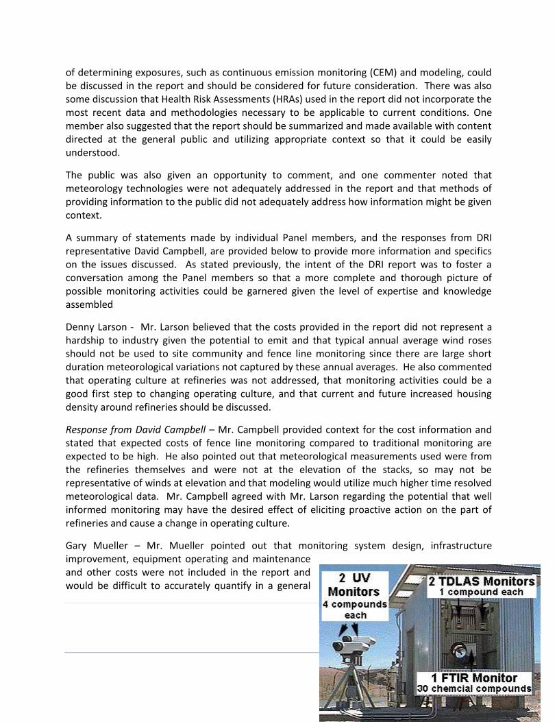
Page 14

of determining exposures, such as continuous emission monitoring (CEM) and modeling, could be discussed in the report and should be considered for future consideration. There was also some discussion that Health Risk Assessments (HRAs) used in the report did not incorporate the most recent data and methodologies necessary to be applicable to current conditions. One member also suggested that the report should be summarized and made available with content directed at the general public and utilizing appropriate context so that it could be easily understood.

The public was also given an opportunity to comment, and one commenter noted that meteorology technologies were not adequately addressed in the report and that methods of providing information to the public did not adequately address how information might be given context.

A summary of statements made by individual Panel members, and the responses from DRI representative David Campbell, are provided below to provide more information and specifics on the issues discussed. As stated previously, the intent of the DRI report was to foster a conversation among the Panel members so that a more complete and thorough picture of possible monitoring activities could be garnered given the level of expertise and knowledge assembled

Denny Larson - Mr. Larson believed that the costs provided in the report did not represent a hardship to industry given the potential to emit and that typical annual average wind roses should not be used to site community and fence line monitoring since there are large short duration meteorological variations not captured by these annual averages. He also commented that operating culture at refineries was not addressed, that monitoring activities could be a good first step to changing operating culture, and that current and future increased housing density around refineries should be discussed.

Response from David Campbell – Mr. Campbell provided context for the cost information and stated that expected costs of fence line monitoring compared to traditional monitoring are expected to be high. He also pointed out that meteorological measurements used were from the refineries themselves and were not at the elevation of the stacks, so may not be representative of winds at elevation and that modeling would utilize much higher time resolved meteorological data. Mr. Campbell agreed with Mr. Larson regarding the potential that well informed monitoring may have the desired effect of eliciting proactive action on the part of refineries and cause a change in operating culture.

Gary Mueller – Mr. Mueller pointed out that monitoring system design, infrastructure improvement, equipment operating and maintenance and other costs were not included in the report and would be difficult to accurately quantify in a general

Page 15

way. He also believed that inventory emissions, especially for particulate matter (PM) may not be representative, especially given that Bay Area plants are gas fired. As a result, the compounds measured need to be correctly prioritized.

Response from David Campbell – Mr. Campbell agreed that the majority of cost information was associated with capital costs and did not include installation and operational costs, as these costs are specific to the facility and difficult to estimate. He also agreed that HRA and emissions estimates should be updated and validated.

Ken Stroud – Mr. Stroud believed that the report should contain a retrospective of the Chevron incident and that continuous emission monitoring (CEM) and source test emission calculations could be used in modeling to estimate exposure.

Response from Air District staff and Denny Larson – Staff and Mr. Larson discussed the various methods used to characterize the Chevron incident. Staff also stated that CEMs located throughout the refineries could be used in various ways to provide information to the public.

Jay Turner – Professor Turner, pointed out the complexity of emissions associated with Bay Area refineries, believed a discussion of the health risk assessment (HRA) should be included to address changes in methodologies that have occurred over time and potential errors inherent in the HRA process.

Response from David Campbell – Mr. Campbell stated that the HRAs were the latest available. He also pointed out that fugitive emissions, which are extremely difficult to quantify, would greatly affect the compound profiles from each refinery and, hence, the type of monitoring needed.

Jay Gunkelman – Mr. Gunkelman believed that while the cost estimate may not include everything, the refineries ability to pay should be included if cost estimates are revised upward. He also pointed out that long-term data from fence line monitoring is available online, though it may be available on other websites. He believed more traditional point source monitoring locations, such as Ground Level Monitors (GLMs), are important to have as a backup to fence line monitoring and that was not addressed in the report. He stated the importance of including both upwind and downwind measurements and provided examples at various Bay Area refineries to illustrate this point. He also believed it important to include a discussion of path length distance associated with open path measurement systems.

Response from David Campbell – Mr. Campbell agreed that upwind and downwind monitors are critical, though with the complex topography and meteorology in the Bay Area, this can be a

Page 16

difficult task to accomplish. He also mentioned the need for highly trained staff to accomplish the majority of measurements discussed.

George Allen – Mr. Allen pointed out that the report may not have addressed the issues associated with appropriate quality control screening as real-time data are made available to the public.

He believed that many alternative methodologies were not addressed in the report and should be considered, examples provided included:

Flux estimate monitoring (open path monitoring with a vertical component in addition to the horizontal component); adequate meteorological monitoring, including measurements at various elevations; video monitoring; seven-wavelength Aethalometers; total sulfur; short term PM measurement; Condensation Particulate Counter (CPC); ThermoScientific PDR and/or ADR 1500, and; SynSpec Benzene, Toluene, Ethyl Benzene and Xylenes (BTEX). He pointed out that equipment and operational costs have been lowered significantly over time and that there are now many sensors available at low cost, though he could not vouch for the accuracy of these instruments.

In addition, he believed that the following issues involving identified methodologies may not have been adequately addressed:

Uptime of Open Path; the costs and benefits of saturation/community scale monitoring; cheaper “do-it-yourself” measurements being investigated by EPA’s Office or Research and Development (ORD). He also cautioned that emissions inventory estimates, especially older ones, tended to underestimate actual emissions, especially those associated with fugitive sources.

Response from David Campbell – Mr. Campbell noted that continuous PM measurements were not covered in-depth in the report and that composition would be needed to determine source. He agreed in general with Mr. Allen’s recommendations for particular instrumentation not included in the report.

Gwen Yoshimura – Ms. Yoshimura suggested that the benefits of identifying specific compounds (tracers) associated with refinery operations and performing tracer studies to aid in modeling and equipment location could be included.

Response from David Campbell – Mr. Campbell pointed out that there are no really well defined tracers associated with the particular individual refineries.

Robert Harley – Professor Harley noted that decreasing concentrations of benzene and associated compounds were likely caused by better mobile source controls, that measuring organic compounds other than BTEX is useful, that higher time resolution for PM measurement

Page 17

was important, that odor and smoke on both a chronic and acute scale were critical to consider and he endorsed using flux estimate monitoring at each refinery.

Andrea Polidori – Dr. Polidori suggested that an Executive Summary of the report be produced for the community and noted that a study of flux estimate monitoring was being performed near a Southern California refinery by UCLA. He also suggested that a combination of monitoring techniques could be employed to provide better overall monitoring, such as using total hydrocarbon measurement to trigger canister sampling for laboratory analysis if measurements exceeded a predetermined level, and methods such as this were not addressed in the report.

Response from David Campbell – Mr. Campbell stated that the report contained only commercially available technologies.

Members of the public – Members of the public believed that human monitoring should be addressed in the report, providing a more holistic approach, that data be presented in a way that the public could understand, that meteorological monitoring in four dimensions be addressed for both fixed and mobile equipment, that trajectory modeling capabilities be addressed, that exposure information be provided, that other agencies be included and that satellite evaluation be considered in the report.

Response from David Campbell – Mr. Campbell provided information requested in email for saturation monitoring which were contained in the report.

Gary Mueller – Mr. Mueller pointed out that there are major differences in flux measurements versus direct concentration measurements and, therefore, there are potentially large, unqualified errors that may be associated with flux emissions estimates, particularly regarding the meteorological components. He also stressed that it is important to concentrate on what measurements are of value to both the community and industry, and that overall monitoring goals need to be well defined.

Page 18

The Expert Panel Addresses Charge Questions

The charge questions the Air District developed for the Panel to consider and member comments are presented below. These comments and input provide a wide range of ideas to consider along with those developed in the DRI report. The Air District intends to use this input to develop guidance for air monitoring activities at Bay Area refineries.

The charge questions considered were:

What should the size and spatial orientation of a network of monitors be around

refineries

What network components should be considered (compounds measured, technology and

instrumentation used, methodologies applied, air quality assessment tools utilized, etc.)

How should the data be provided to the public

What should be considered when developing measurement quality objectives, such as:

o What type of instrument siting criteria should be used

o What should the time resolution of the equipment be

o How often should the instrumentation be calibrated

o What should the accuracy/precision/completeness requirements of the data be

o What other quality control/quality assurance requirements should be put in place

What technologies, methodologies and tools could be employed to augment any fixed

network to better quantify pollutant variations over space and time, especially during

short duration incidents

What emerging technologies might be utilized in the future to further enhance

community air monitoring capabilities

Summary of Comments

In general, the Panel agreed that a combination of measurements would be required to adequately provide the public with information regarding emissions from refineries in the Bay Area. Members generally agreed that fence line monitoring, particularly open path monitoring that provided information along refinery boundaries, was useful. However, these systems did not provide information about actual community exposures and concentration gradients as distance from fence lines increased. Therefore, monitoring within the community was necessary to capture this information. Members generally agreed that this community monitoring would require a flexible approach with a combination of traditional, fixed-site regulatory air monitoring and more dense, lower cost methods that would allow for better spatial coverage. This coverage should utilize a “layered” gradient approach that focused on near source measurement to help define concentration gradients. During incidents and upsets,

Page 19

it was recognized that a fixed network would likely not adequately characterize localized and highly variable exposures and that mobile monitoring would be the best methodology to capture these emissions. There was also discussion of the usefulness of emission flux measurements to determine the accuracy and variability of emissions inventories. Most Panel members agreed that the DRI report provided appropriate information on the various general techniques available with the appropriate goals and strategies identified in both the report and presentation provided.

The Panel also discussed and generally agreed that compounds of interest should be identified and investigated with relationships and correlations developed to better identify appropriate monitoring goals. It was also generally recognized that not all compounds of interest should be measured, that volatile organic compounds (VOC) should be the primary focus, and that every in-place, available resource should be utilized and/or leveraged to provide information to the public, such as the existing air monitoring network, CEMs and HRAs.

The Panel generally agreed that the data collected should be provided to the public through an easily understood web interface with appropriate context provided. However, alternate methodologies should also be developed to inform members of the public who lack computer access or need additional information. The context should include ways for the public to compare measurements to other locations and to appropriate health indicators and to recognize when values were below instrumentation’s level of detection. In addition, there should be ways for more sophisticated users to access and download more complex and/or historical data. Most members of the Panel indicated that the website should employ ways for the public to provide information back to industry and the Air District regarding their experiences and observations. There was much discussion about how to address data quality and the removal/notation of data that did not meet desired quality bench marks. Most members agreed that data completeness was critical, with some members of the Panel representing the community being less concerned about issues arising from data quality.

The Panel generally agreed that higher time resolution was desirable, with the recognition that time resolution and accuracy needed to be appropriately balanced. It was also generally agreed that time resolution depended upon the monitoring goal associated with the measurement and that some flexibility should be developed to address this issue. For example, fence line monitoring should have a higher time resolution, on the order of five minutes, while community monitoring of chronic exposures could have times on the order of hourly, or daily, depending on the monitoring need. However, during incidents or upsets, the community monitoring time resolution should be increased to represent more acute exposures and mobile monitoring should have the highest time resolution possible to address acute exposures and spatial variability. Most Panel members believed the Air District along with instrument manufacturer recommendations would be adequate to determine additional data quality issues.

Page 20

Members of the Panel generally agreed that periodic review of applicable technologies would be required to ensure that the best techniques were utilized. In addition, Panel members agreed that lines of communication should be fostered to ensure transparency and trust.

What should the size and spatial orientation of a network of monitors be around

refineries

Participants agreed that fence line monitoring in addition to community monitoring be employed. Fence line monitoring should cover the majority of refinery/community interface as possible. They provided the following comments on the community monitoring portion.

Jay Turner – Professor Turner stressed that the appropriate size and spatial orientation of any monitoring network depends on many variables; especially the desired compounds being measured, their relationship to emissions from the refinery and the changes in concentration with increased distance from the source. For example, he noted that particular point sources, such as delayed cokers and catalytic crackers would require a very focused monitoring approach if metals were the targeted compounds, while focusing on hydrocarbons would require a very different approach.

George Allen – Mr. Allen suggested that a “layered” approached should be utilized in which gradients are measured based on a limited number of fixed sites with accurate, stable and continuously operated instrumentation followed by “layers” of more spatially dense measurements that provided better spatial coverage designed to provide more information, potentially sacrificing accuracy or other measurement characteristics to lower costs based on the overall monitoring goal. Panelist’s widely agreed that this was a desirable approach.

Jay Gunkelman – Mr. Gunkelman stressed that each refinery be evaluated separately since each facility has unique characteristics.

Gary Mueller – Mr. Mueller stated that the current air monitoring network for NOx, PM and SO2 probably does an adequate job. For VOC’s, there is likely room for improvement. So while there are many compounds that may be impacting the community, the focus should be on those that are more known and likely to have impacts, while other, less obvious compounds potentially being the focus of limited investigations prior to a more widely deployed network.

Denny Larson – Mr. Larson agreed with the above approaches and stressed that community involvement would be a good starting point to base investigations of less obvious compounds on, focusing on symptomatic and odor log observations by the community. The involvement of the community in the process should be ongoing to capture changes in refining processes over time.

Page 21

Robert Harley – Professor Harley stressed that visual and olfactory information collected by the community was important and need not involve expensive equipment or large amounts of technology to accomplish.

Jay Turner – Professor Turner stressed the importance of identifying gradients by measuring in areas that had not been included in the past and relating those measurements back to longer term measurements in the area, providing an idea of scale of impacts and context to measurements. He pointed out that measuring close enough to the sources with appropriate spacing between measurements to fully capture gradients was the key (capturing the “zone of influence”). He also stressed that a representative background site near the refineries was critical to understanding localized concentrations since emissions from refineries mimicked mobile sources in many, surprising ways. He also believed that a gradient/saturation or “layered” approach was appropriate.

Ken Stroud – Mr. Stroud agreed with Professor Turner that a gradient, saturation approach as described by the DRI report was best.

Andrea Polidori – Dr. Polidori stated that budgets need to be defined up front to ensure that adequate sampling is performed prior to funding being exhausted. He also stated that time resolution and capture of seasonal variation was the biggest obstacle to overcome with a gradient approach.

Gwen Yoshimura – Ms. Yoshimura agreed with the above approaches and that a combination of all of the above methods should be employed.

Jay Turner – Professor Turner believed that saturation monitoring could inform the location of more permanent sites and that those site should be located quite near the facilities (within blocks). He believed that no more than three permanent sites should be considered with one of those sites being a “background” site.

Thomas Kirchstetter – Dr. Kirchstetter cautioned that shorter duration monitoring could be problematic due to seasonal variations in meteorology and that these factors must be considered when shorter term studies are developed.

What network components should be considered (compounds measured, technology

and instrumentation used, methodologies applied, air quality assessment tools

utilized, etc.)

Jay Turner – Professor Turner stressed that VOC’s are the logical starting point for any study and refinery-to-refinery variation should be identified, if possible. Once VOC relationships and correlations are developed, limiting the number of compounds measured would be a good way to limit costs. He also believed that use of real-time instrumentation was best suited to identify

Page 22

correlations and unique variations. He stressed that speciation of hydrocarbons (such as what field gas chromatographs/SynSpec-like equipment would supply) are well suited for these purposes.

George Allen – Mr. Allen agreed that VOC’s should be included and limited to identified “indicators”, but also believed sulfur compounds should be used as indicators, especially since most open path equipment respond well to these compounds. He also identified formaldehyde as an example of a risk driver that should be measured, but that it is extremely difficult to measure well. He felt that passive sampling for VOC’s, such as canisters, should be triggered by total non-methane hydrocarbon (TNMHC) measurements. He identified ammonia as a compound that is easily measured using passive technologies, but difficult to measure continuously. He used these examples to demonstrate the complexity and difficulty in designing community monitoring networks and the need for a flexible approach.

Gary Mueller – Mr. Mueller pointed out that PM measurements at natural gas fired refineries are not effective during normal operation due to the low amount of PM directly emitted. Measurements of NOx and SOx are performed largely at emission points and probably do not need to be addressed offsite. Identifying the monitoring goal and identifying the impacted areas not addressed by historical monitoring is the first place to start.

Jay Gunkelman – Mr. Gunkelman stressed that upwind and downwind measurements were critical and that specifics and uniqueness of site locations were important to consider, especially during divergent seasons. He believed 10-meter meteorological towers provided the most representative information. He also believed that limiting the number of compounds to include only the most important was necessary, but that at least one compound (for example, carbon tetrachloride) should be used to serve as a background QA/QC check.

Robert Harley – Professor Harley supported the use of radar profilers for meteorological measurements and also believed that flux estimate monitoring was ideal to validate emissions inventory estimates, providing a more realistic estimated community concentration and an ideal starting point for identifying community monitoring needs. He also reminded everyone that PM measurements while potentially not an issue during normal operation, was important during upsets and incidents.

Page 23

George Allen – Mr. Allen believed that sodar was a good methodology to employ to estimate mixing heights. He also added that if methane and TNMHC measurements were made, that the methane measurements would be a good QA/QC check of the TNMHC data.

Denny Larson – Mr. Larson believed that PM should be included in any network design and that polycyclic organic hydrocarbon compounds (PAHs) should also be considered in the event of fallout from upsets and incidents. He also believed measurements at elevation should be considered to capture buoyant emissions. Mr. Larson also believed analysis of past incidents and upsets were critical to inform future actions.

Jay Turner – Professor Turner stressed again that identification of compound relationships and correlations in conjunction with potential facility uniqueness should be the starting point for VOC measurement. He also agreed that carbonyl measurement is desired, but difficult, and supported the use of UV DOAS instrumentation based on its potential ability to measure carbonyls.

Gwen Yoshimura – Ms. Yoshimura noted that a Beta Attenuation Monitor (BAM) is now in place at the San Pablo air monitoring station as well as other Bay Area locations and these instruments are now producing hourly PM data. She also stated that data quality and presentation to the community must be considered along with everything else.

How should the data be provided to the public

Denny Larson – Mr. Larson stated that all available air quality data the Air District is responsible for should be provided along with context and a feedback mechanism. He believed that the fence line monitoring systems at Crockett and Rodeo are good models. He also reminded that there are methods other than the internet to provide the information to the public.

Jay Gunkelman – Mr. Gunkelman stressed that feedback to public input must be instantaneous and thorough and that the GLM data need to be posted online. Website graphical interfaces need to be simple and provide general information that is easily understood.

George Allen – Mr. Allen pointed out that data should be web-based along with an alternative, such as a telephone hotline, for those without computers. The web-based data should be “layered”, so that people with rudimentary knowledge have a page and that people who wish more complex data, such as researchers, can get more complex data. He noted that there is a great deal of meteorological data available through other sites, such as Weather Underground. Data should also be tied to risk and/or exposures.

Jay Turner – Professor Turner suggested that context be provided with a baseline reference (either regulatory or “normal” concentration) with comparisons to other Air District/State sites. He stated that AirNow is a good model.

Page 24

Gwen Yoshimura – Ms. Yoshimura suggested that a feedback loop be developed between the refineries and community so that there are defined actions taken when certain concentrations are reached. These levels and actions should be communicated so that the public knows that there are actions associated with the data. She supported the multilevel approach and reminded that download speeds should be considered.

Ken Stroud – Mr. Stroud suggested that data also be shared with websites that display national data, such as AirNow, and state sites, such as AQMIS, so that the public can get everything they need at one location.

Andrea Polidori – Dr. Polidori suggested that there be consideration for allowing a time period between when the data are collected and when they are displayed to the public to allow for appropriate quality assurance (QA) activities to be completed, if necessary. He provided the example of laboratory analysis that would require additional time. He also suggested that there be a tie-in between measurements and health consequences, if possible, potentially utilizing real time health measurements (though that may not be quite ready yet).

George Allen – Mr. Allen stated that he believed missing data had the potential to raise trust issues and that transparency was the answer to these issues. A mechanism to explain why data are missing should be provided, such as meta data and performance parameters outside of which data are not valid. In addition, clearly identifying what is displayed when values are below the instruments limit of detection (LOD) is important.

Gary Mueller – Mr. Mueller suggested that all data be displayed and labeled to indicate potential issues with data quality, though he was not sure how that might be accomplished.

Denny Larson – Mr. Larson stated that data quality is not an issue as long as real-time results are displayed and available, with QA activities and data reporting that requires additional time achieved quickly. He believed that reliability and up-time were the more critical issues and that 99% data completeness should be the goal. Any corrective action should be taken quickly and feedback mechanisms, such as blogs and bulletin boards, should be employed to provide a venue for sharing information and suggesting improvements.

Thomas Kirchstetter – Dr. Kirchstetter pointed out that web pages should initially provide straightforward information with the ability to get additional, more complex data built in. He believed that the current Air District website was a good starting point, but that it needed to be improved. Having the ability to plot data in graphical format would potentially enhance understanding. Dr. Kirchstetter also believed that displaying data with the correct level of precision was important and that using “<LOD” when concentrations were below instrumentations LOD would be the best method as long as LODs were provided.

Page 25

Jay Gunkelman – Mr. Gunkelman agreed with Mr. Larson that removal of data that didn’t meet quality assurance requirements was not an issue as long as high rates of data completeness were maintained. He supported the use of “<LOD” for values below detection levels. His main concern was the robustness of the website and the defensibility of the data. Traffic to the website could also be used as a means of measuring whether problematic issues were occurring.

Jay Turner – Professor Turner believed that issues around data quality would be addressed quickly if all refineries are performing similar measurements, the data stream is monitored and feedback around missing data or data outliers are addressed.

George Allen – Mr. Allen stated that urban background numbers should be provided to give context to the concentration numbers and associated risk.

What should be considered when developing measurement quality objectives, such as:

o What type of instrument siting criteria should be used

o What should the time resolution of the equipment be

o How often should the instrumentation be calibrated

o What should the accuracy/precision/completeness requirements of the data be

o What other quality control/quality assurance requirements should be put in

place

Denny Larson – Mr. Larson stressed the importance of good siting and that elevation, especially for fence line monitoring, is an important consideration. He also stressed that community monitoring should take place in impacted communities, and that compromises for power and security should be less of a consideration than appropriate location within the community.

Jay Gunkelman – Mr. Gunkelman stressed the need for short time resolution, especially at the fence line (5 minute). He stated that the vendor instrument operational recommendations should drive QA requirements. Data completeness for components and the overall system should be 95%.

Robert Harley – Professor Harley agreed that one hour time resolution is the minimum acceptable time frame. Backup power should

also be a serious consideration.

Ken Stroud – Mr. Stroud stated that the Air District should have oversight of the QA processes, which the Air District supports.

Page 26

Jay Turner – Professor Turner made the point that time resolution could be varied according to the major goal of the monitoring. During upsets, for example, time resolution should be increased. This may result in a decrease in accuracy, but this may be an acceptable trade off during short term events when acute exposures are more important. For more chronic exposures, accuracy becomes more of a driving force and time resolution of an hour is more acceptable.

George Allen – Mr. Allen supported the view expressed by Professor Turner, that time resolution and accuracy should be based on the importance of the exposure (chronic versus acute).

Andrea Polidori – Dr. Polidori stated that it was better, in his opinion, to delay posting of data so that quality was ensured and data would not have to be removed at a later date, potentially causing trust issues. He also stressed that co-location of instrumentation would need to be considered to provide information on overall data quality.

Gwen Yoshimura – Ms. Yoshimura stressed that community involvement was critical and that they should be involved in determining how to balance time resolution and accuracy.

What technologies, methodologies and tools could be employed to augment any fixed

network to better quantify pollutant variations over space and time, especially during

short duration incidents

Thomas Kirchstetter – Dr. Kirchstetter thought sampling during incidents could be modified to address the shorter duration of incidents, especially those at permanent locations near facilities. For example, canister samples, which are traditionally collected over 24-hours, could be collected every three hours for 24 hours during the event and used to compare to the more traditional sampling. This would provide flexibility and potential cost savings.

Denny Larson – Mr. Larson was not sure if the technique described by Dr. Kirchstetter should be employed. He believed this to be was more of an issue with the goal of the sites (ambient versus incident related). He suggested that monitoring near facilities should follow a different siting criterion. Siting for incidents should be mobile, as opposed to fixed, as this would be the best way to “track” impacts.

George Allen – Mr. Allen supported mobile monitoring during incidents which would augment the fixed network. Time resolution of a minute, maximum, should be employed with the ability to grab canister samples when direct reading instruments indicate high concentrations. He believed this may also be a situation to employ the semi-quantitative Ecochem PAH instrument (fast response and easy to run). This should be tied to real time meteorology and modeling.

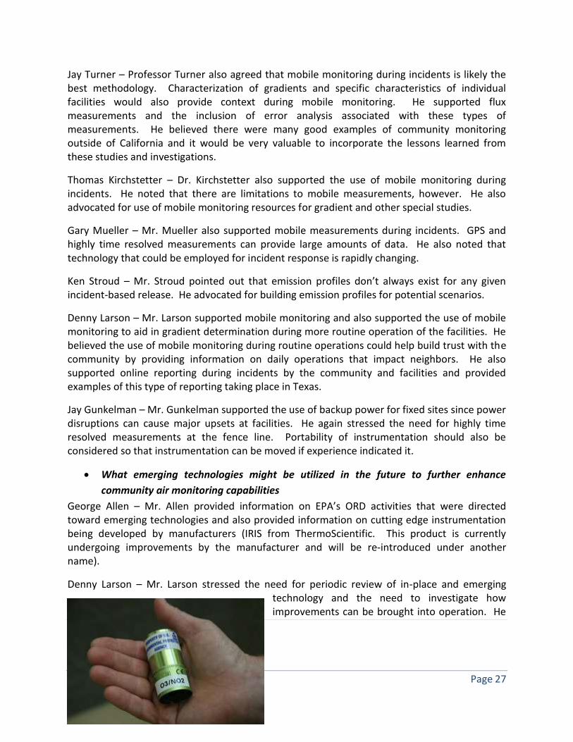
Page 27

Jay Turner – Professor Turner also agreed that mobile monitoring during incidents is likely the best methodology. Characterization of gradients and specific characteristics of individual facilities would also provide context during mobile monitoring. He supported flux measurements and the inclusion of error analysis associated with these types of measurements. He believed there were many good examples of community monitoring outside of California and it would be very valuable to incorporate the lessons learned from these studies and investigations.

Thomas Kirchstetter – Dr. Kirchstetter also supported the use of mobile monitoring during incidents. He noted that there are limitations to mobile measurements, however. He also advocated for use of mobile monitoring resources for gradient and other special studies.

Gary Mueller – Mr. Mueller also supported mobile measurements during incidents. GPS and highly time resolved measurements can provide large amounts of data. He also noted that technology that could be employed for incident response is rapidly changing.

Ken Stroud – Mr. Stroud pointed out that emission profiles don’t always exist for any given incident-based release. He advocated for building emission profiles for potential scenarios.

Denny Larson – Mr. Larson supported mobile monitoring and also supported the use of mobile monitoring to aid in gradient determination during more routine operation of the facilities. He believed the use of mobile monitoring during routine operations could help build trust with the community by providing information on daily operations that impact neighbors. He also supported online reporting during incidents by the community and facilities and provided examples of this type of reporting taking place in Texas.

Jay Gunkelman – Mr. Gunkelman supported the use of backup power for fixed sites since power disruptions can cause major upsets at facilities. He again stressed the need for highly time resolved measurements at the fence line. Portability of instrumentation should also be considered so that instrumentation can be moved if experience indicated it.

What emerging technologies might be utilized in the future to further enhance

community air monitoring capabilities

George Allen – Mr. Allen provided information on EPA’s ORD activities that were directed toward emerging technologies and also provided information on cutting edge instrumentation being developed by manufacturers (IRIS from ThermoScientific. This product is currently undergoing improvements by the manufacturer and will be re-introduced under another name).

Denny Larson – Mr. Larson stressed the need for periodic review of in-place and emerging technology and the need to investigate how improvements can be brought into operation. He

Page 28

also stressed that communication between government, the facilities and the community is critical to continue over time.

Gary Mueller – Mr. Mueller pointed out that there are numerous technologies that need to be investigated, tracked and potentially installed, but it is important to consider that any technology needs to be tested and evaluated thoroughly prior to use to inform the community.

Members of the Public – Members of the public stressed that it is important that government agencies respond to complaints so that the community knows that their observations are being recognized and investigated. The data needs to be made understandable to the public and context must be provided to ensure that the effort provides value to the community. The public would like to focus on preventative actions. Online information, such as wikis should be considered. Members of the public supported providing an explanation of why data are invalidated. The public also supported the development and dissemination of emission profile information, the use of video monitoring and the investigation of better manufacturing processes that reduce emissions.

The Panel provides their final thoughts

Robert Harley – Professor Harley stated that whatever actions are taken, they must provide value to the various stakeholders.

Denny Larson – Mr. Larson pointed out that his principals for air monitoring that were provided to the Panel would be a good starting point for any future discussions.

Jay Turner – Professor Turner stressed that the DRI report provided the appropriate five objectives to consider for additional network development and the emphasis of those objectives will be based on policies developed by the Air District through the various inputs, including the Panel and the community.

Gwen Yoshimura – Ms. Yoshimura reminded that the data can have many uses, including uses for the refineries that should use the data to make improvements to their processes proactively.

Gary Mueller – Mr. Mueller stated that continuing communication between all parties is important and should continue to be developed and supported. He also fully supported the use of mobile monitoring during incidents, especially monitoring of PM.

George Allen – Mr. Allen stated that near-field data was of high value, especially to industry. He noted that there have been improvements, but that tools such as video can be quite valuable to both the community and industry.

Page 29

Jay Gunkelman – Mr. Gunkelman stressed the value of community/government/industry interaction during any process. He was encouraged that monitoring will be taking place at refineries throughout the Bay Area.

Andrea Polidori – Dr. Polidori agreed that good communication is required for any effort to be successful. He suggested that there are practices in place in the South Coast Air District, such as email notifications of planned and unplanned flaring events that could be incorporated in the Bay Area.

Page 30

Panelists Response to Comments –

Members of the Panel were given an opportunity to provide clarification to comments attributed to them and were incorporated into this report. Panel members were then given another opportunity to provide comments on the DRI report not captured above, and comment on input from other Panel members. All input is provided below.

Mr. Denny Larson provided comment:

“We need to make clear that the process of doing these tasks should model what is done with the GLM monitoring network. That is the District provides a general outline for installing the network and provides specific recommendations for equipment. Then it is up to the refinery to install and contract out the operation of the equipment.

The Air District needs allow the refineries to make available to the public the GLM data that is currently being generated immediately. It costs nothing and provides an immediate public good. Again the key would be to let the refineries make it public, not the air district.

Have each refinery set up a process by which it makes public its data. This should also include input/feedback and participation from local communities. It's better to provide local input as compared to a process where a central authority makes all decisions.

The fence line monitor success for 20+ years in Rodeo at Conoco is due in large part to the local community working group working with the refinery and the relevant agency. The District's policies and rules in this regard should require a local working group of refinery neighbors.”

Professor Robert Harley provided comment:

My comments “are all mentioned in the draft report already, but I want to emphasize/elaborate on some key points.

1. That solar occultation or similar open-path techniques be used to survey baseline emissions from each refinery under normal operating conditions (this can be used to check the District's emission inventory; there may be uninventoried fugitive sources of VOC emissions especially).

2. That District monitoring efforts relating to abnormal events/upsets at refineries include measurements of ambient particulate matter using online methods that provide at least hourly updates to the data. Such data on PM mass (measured, for example, by beta attenuation) could be useful in identifying smoke plumes that arise due to fires or large flaring events at the refineries. Fence line and community monitoring efforts seem heavily focused on measuring gaseous pollutants.

Page 31

3. Earthquakes are a known hazard in the Bay area, and both refinery systems and BAAQMD monitoring capabilities should be assessed for safety and resiliency in the face of extended outages in electric power and other lifeline systems (water supply, transportation, communication, natural gas) that may ensue.

4. Enhancements to meteorological data collection (e.g., from one or a few radar wind profilers operating continuously) may help the District assess the transport and magnitude of air pollution plumes from refineries, as well as impacts on nearby communities. Such data may also serve other District needs such as air quality modeling and planning efforts.”

Mr. Ken Stroud provided comment:

“I have reviewed the report, “Air Monitoring Technology and Methodology Expert Panel Report and Findings,” and find that it adequately captures my input to the Panel Discussion of July 11, 2013.”

Dr. Andrea Polidori provided corrections/clarifications to comments attributed to him which have been incorporated into this report and also provided comments on the DRI Report, which will be forward to the author of that report for editing consideration.

Mr. George Allen provided corrections/clarifications to comments attributed to him and have been incorporated into this report.

Page 32

Panelists Written Comments –

District staff invited Panelists to provide additional written comments after the meeting to address the charge questions and provide additional insight. These are attached, represent the position of the Panelist, and have not been edited by Air District staff.

Response to Charge Questions to the Air Monitoring Technology and Methodology Expert Panel

DRAFT – George Allen July 17, 2013

Q 1: What should the size and spatial orientation of a network of monitors be around

refineries

A network of fixed sites should have multiple layers to meet the multiple objectives needed to

properly assess source emissions and population exposures both for routine (normal) operating

conditions as well as abnormal emission scenarios.

1. Near-field source characterization measurements. This component of the network is designed

to measure pollutants at or near the fenceline (up to ~ 100 m away), and potentially at different

heights above the ground. Open path methods are most appropriate here, but not necessarily

located on or near the ground. Near-field sampling should be located at heights that are relevant

to the structure of the refinery and known or likely emission sources). These measurements

would ideally be located both up- and down-wind of the refinery (using prevailing wind

directions).

2. Mid to neighborhood-scale fixed sites with full instrumentation. These sites would be the

backbone of a long-term network with multiple measurements, including both real-time and

integrated sampling. These sites would be between 500 to ~2000 m from the fenceline, and

provide detailed and high quality data for routine (non-event) conditions that could be used for

assessment of chronic health risks. Depending on resources, this could be a single down-wind

site or include several down-wind sites and a single up-wind site. These fixed sites should be

located at the most likely high-concentration area, determined by dispersion modeling using

appropriate on-site wind fields at multiple elevations if possible. One potential routine use of the

data from these sites would be to ground-truth refinery emission inventories. These have been

shown to sometimes be substantial under-estimates of true facility emissions due to the potential

for a large number of unidentified fugitive emission sources. See:

Henry, R.C., Spiegelman, C.H., Collins, J.F., EunSug Park (1997). “Reported emissions of

organic gases are not consistent with observations.” Proceedings of the National Academy of

Sciences of the United States of America, Vol. 94, 6596–6599.

http://www.pnas.org/content/94/13/6596

and

Page 33

Ryerson, T. B., et al., Effect of petrochemical industrial emissions of reactive alkenes and NOx

on tropospheric ozone formation in Houston, Texas. J. Geophys. Res., 108(D8), 4249,

doi:10.1029/2002JD003070, 2003. Report at:

http://www.researchgate.net/publication/225089790_Signatures_of_terminal_alkene_oxidation_i

n_airborne_formaldehyde_measurements_during_TexAQS_2000/file/9fcfd51072f40594aa.pdf

3. Mid to neighborhood-scale fixed sites with limited instrumentation. These sites would be

simpler and lower cost, to provide additional spatial information on a limited number of indicator

pollutants. Passive or low-cost real-time sensors would be used at these sites. One of these sites

should be collocated with a fixed site described in #2 above for QC purposes. One should be up-

wind of the refinery.

Q 2: What network components should be considered (compounds measured, technology

and instrumentation used, methodologies applied, air quality assessment tools utilized, etc.)

For near-field open path measurements, indicator pollutants are appropriate. These could include

methane, benzene or other BTEX VOCs, SO2, or other relevant pollutants. NOx and PM do not

need to be measured.

For the larger fixed site monitoring locations (Q1 #2 above), the following measurements should

be considered, roughly in order of importance:

Real-time BTEX (Synspec or similar) with 5 to 15-minute resolution

SO2 and total gas-phase sulfur (e.g., reduced S compounds) with 5 to 15-minute resolution

Methane and total non-methane HC with 5 to 15-minute resolution

Optical Black Carbon (BC). The new version of the Magee/TAPI model AE33/633 Aethalometer

addresses the limitations of “legacy” Aethalometers, including noisy short-term measurements

and “spot-loading” effects. The instrument provides stable data with high time resolution (1-

minute or less) over the range of 950 to 370 nm, with 1-minute LOD of ~ 50 ng/m3. Enhanced

response at 370 nm relative to 880 or 950 nm is a specific and semi-quantitative indicator of

cellulose combustion.

Particle number concentration (PNC or UFP) down to < 10 nm is readily measured with the TSI

3783 CPC (TAPI model 651) with rapid response time and high sensitivity. PNC along with

time-resolved and sensitive PM2.5 (pDR-1500) can give an indication of the age of the aerosol;

high PNC with relatively low mass is typical of very fresh combustion, while relatively low PNC

and high PM2.5 indicates an aged aerosol.

Page 34

Automated GCs can provide speciated VOCs with high time resolution; these data can be useful

to ground-truth total VOC emissions from large facilities as noted in Q1, #2 above).

NH3 (resolution TBD based on method – electro-chemical for higher “event” concentrations ~1

ppm and up)

Meteorology:

10 meter wind with 5 to 15-minute resolution

Ceilometers give a useful measurement of mixing height up to ~ 5 km and are relatively simple

and inexpensive compared to radar/profiler systems. Example:

http://www.vaisala.com/en/products/ceilometers/Pages/CL31.aspx

Highly time-resolved (1 to 5-minute) PM2.5 (e.g., optical methods supported by BAM or TEOM

measurements that only provide hourly PM data. The Thermo pDR/aDR1500 has been shown to

provide useful measurement of PM2.5 at 1-minute or less time resolution: http://www.thermoscientific.com/ecomm/servlet/productsdetail_11152_L11082_89583_11961321_-1

NO and NO2 (1 to 5-minute resolution)

The EcoTech PAH analyzer provides qualitative highly time-resolved measurement of particle-

bound

PAH. While data quality is not high, the method is inexpensive and easy to run.

http://www.ecochem.biz/PAH/PAS2000.htm

Canister measurements of VOCs, both routine (every x days) and possibly event-triggered

samples driven by the TNMHC real-time measurements. Similar event grab samples could be

taken using the SO2/TS real-time measurements.

The less intensive fixed sites could include passive measurements of VOC, SO2, and possibly

NH3; the two major suppliers of passive samplers and related chemistry are noted in the DRI

report. PM2.5 could be measured using optical scattering methods such as the self-contained

Thermo aDR-1500. Electro-chemical sensors are available for many gases, including CO, H2S,

chlorine, ClO2, mercaptans, HCl and others; this technology has dramatically improved over the

last decade, with improvements in baseline/temperature drift. One leading manufacturer of high

quality electro-chemical cells is City Technology in England:

http://www.citytech.com/

Q 3: How should the data be provided to the public

A web site should be used to provide data to the public. There are several key components of a

web site for this purpose:

Page 35

1. A layered approach to data and interpretation that allows the user to “drill down” to the

desired level of detail. The top layer would be simple, non-technical information, using

messaging similar to the AQI (colors and descriptors) and indicate if conditions are normal or

not. The second layer could include more pollutant-specific information (including health

effects). The third layer would provide access to current and historical data and more detailed

information on health effects, both chronic and acute. All layers should present information in a

spatial context. For example, clicking on a site on a map leads you to the next layer of data.

2. It is critical that data from refinery network monitors be put in context with similar data from

urban-scale contemporary measurements, since source-profiles from refineries under normal

operating conditions are usually similar to ubiquitous mobile-source air toxics such as benzene.

This would require measurements of key real-time pollutants at an urban site not influenced by

refinery emissions. Data for all layers of the web site could be presented as “excess” over urban

background, either alone or (for the third layer) with the actual concentrations from near-refinery

and urban background monitoring sites. This is a health “risk communication” issue,

acknowledging that there is some risk even during normal conditions and at urban background

concentrations.

3. Data must be “time-relevant”. For routine measurements (and non-event conditions), hourly

data is sufficient. But during an event, data must be updated at least every 5-minutes, and ideally

every minute when levels are elevated. While instrument uncertainty (LOD, noise, etc) decreases

at very short time intervals, the periods when high-time resolution is needed would be when high

concentrations of pollution are present. Some degradation in data quality is an acceptable trade-

off for high time resolution during these event conditions.

4. “Missing” data must be addressed in a transparent manner. Why it is missing (specific

information, not just “invalid data” and (for real-time data) when it is expected to be available

again is key information that must be provided.

5. Data quality indicators should be included in some manner at all levels of the web site. For

transparency, data below LOD should be shown with suitable data quality indicators. Colors or

text size, etc. could be used to mark data of inadequate quality, with the reason noted.

6. To the extent possible, web pages should be ADA-compliant, or an ADA-compliant version of

the web site should be provided even if it has limited information relative to the main site. The

web site should be designed to be easy to view for those with some vision impairment. This

means NO low-contrast layout [e.g., no light blue on darker blue] - information should be black

on white wherever possible. Users should be instructed on how to enlarge the page in the

browser (View/zoom, or Ctrl +, -, and 0).

7. The web server must be capable of handling very large traffic that would likely occur during a

substantial event – when the site is most needed. Below is an example of traffic to hazecam.net

Page 36

when superstorm Sandy hit the NY/NJ coast on Oct. 29, 2012; this demonstrates the relative

traffic during an event of note.

8. Web access can not be assumed. A telephone (toll free?) hotline should be part of the data

access system. Information on the hotline would be limited, similar to level 1 of the web site, and

presumably limited to a single location unless all locations are “normal”. Users could enter a zip

code or other geographical locator information such as the name/town of the refinery of interest

when conditions are not normal. A telephone contact number for additional information during

times when conditions are not normal should also be provided.

Q 4: What should be considered when developing measurement quality objectives, such as:

– What type of instrument siting criteria should be used

This is covered under the first charge question.

– What should the time resolution of the equipment be

This is covered under the second charge question.

– How often should the instrumentation be calibrated

For methods that the US EPA has established QC guidelines for, those guidelines should be

followed. For other methods, good laboratory practice should be followed, taking into

consideration the level of data quality needed and the stability of the method.

– What should the accuracy/precision/completeness requirements of the data be

Accuracy and precision are most important when normal (non-event) conditions are present and

hourly data and data “higher than urban background” are the primary products. As noted above,

precision is less important when elevated levels are present and a trade-off between precision and

high time-resolution is needed. Completeness is the most important requirement. Routine

measurements normally have minimal missing data beyond precision/calibration/maintenance

outages. Some methods such as open-path instruments may have substantial missing data due to

the complexity of the method. If high data capture is important for these methods, appropriate

resources must be made available.

– What other quality control/quality assurance requirements should be put in place

Page 37

To the extent possible, “buddy-system” checks may provide useful data quality information

during routine (non-event) monitoring.

Q 5: What technologies, methodologies and tools could be employed to augment any fixed

network to better quantify pollutant variations over space and time, especially during short

duration incidents

Rapid deployment of mobile measurements are critical to provide detail on areas of maximum

concentrations. The mobile platform must have very highly time-resolved measurements of key

indicator pollutants – one minute or less if possible. In addition to methods noted above, portable

photo-ionization detectors (PID) instruments may provide useful data for mobile use.

Real-time dispersion modeling along with the real-time fixed monitors could be used to

determine the most likely area[s] of maximum concentrations. To maximize the accuracy of the

dispersion modeling, wind data at multiple levels at or just down-wind of the refinery are

needed, from 10 meters to stack-top elevation, including

30 and possibly 100 meter wind. Multiple elevations are

essential since wind direction can change dramatically

over several hundred feet as shown in this classic picture

by Bruce Egan of the Salem (MA) Harbor coal-fired

EGU. The coastal meteorology present at these refineries

further complicates estimation of plume impacts using

dispersion modeling. These wind measurements should

be “3D” sensors that include the vertical wind component. Wind data must be highly time-

resolved – 1 minute or less, with vector averaging up to longer time-scales (e.g., 5, 10, 15

minutes or more).

Another source of surface wind data that may be useful during an event is the dense “network”

of personal weather stations (PWS) that report to organizations such as the Citizen’s Weather

Observing Program (CWOP). These data go into the NOAA Meteorological Assimilation and

Data Ingestion System (MADIS) where they are QC’s using a “buddy-system” approach. The

data and related QC parameters are “exposed” by CWOP. See a presentation I gave at the 2009

EPA national monitoring conference:

http://www.epa.gov/ttn/amtic/files/2009conference/AllenFreeMetQC.pdf

Some PWS only report to weather underground and do not receive MADIS QC; all CWOP sites

appear on weather underground, identified as APRSWXNET for the data source and with site

IDs consisting of M and a single letter ©, D, or E) followed by four digits. Example: MD2257. A

list of public stations sending data into MADIS from many different mesonets (CWOP is one of

many) is at: http://madis.noaa.gov/public_stntbl.csv

Weather underground provides maps of station locations that link directly to a station’s data:

http://www.wunderground.com/wundermap/?lat=37.94056&lon=-122.34944&zoom=12

Page 38

Data are also available from the MesoWest database:

http://raws.wrh.noaa.gov/cgi-bin/roman/meso_base.cgi?stn=D2257&unit=0&time=LOCAL

Another “measurement” that may be useful is automated photography. Properly sited high

resolution cameras (not “web-cams”) could be used to track and document plume location,

dispersion, and elevation during an event (the pictures from the August 2012 event demonstrate

the value of this approach). These cameras could be both visual and infra-red (for night-time

use). Ideally each refinery would have three cameras providing views from a few miles away

from three angles of view to allow triangulation of any visible plume. A camera network could

be part of the web-site (a valuable outreach tool), and could capture smaller events that may not

be picked up by the routine monitoring network. A network of “visibility” cameras I run in the

northeast US has captured several notable pollution events (including the direction and intensity

of the 9/11 NYC plume), and has been used as part of an enforcement action against an EGU in

the Boston area by the US EPA. See: www.hazecam.net . Mexico City has a “hazecam” looking

at Popocatepétl:

http://148.243.232.113:8080/calidadaire/vigilancia_cam/hazecams.php

Q 6: What emerging technologies might be utilized in the future to further enhance

community air monitoring capabilities

There are some key pollutants that are difficult to measure, such as carbonyls, especially HCHO

and acetaldehyde. At present, even routine integrated measurement of these carbonyls (using

DNPH cartridges) is difficult; optical (open path) methods are the only reliable technique.

Carbonyl source profiles may be very different than the more common MSAT-related pollutants,

making them important pollutants to measure. There is at least one promising technology under

development. Thermo has their “IRIS” system that uses mid-IR spectroscopy to measure

methane, CO, CO2, and N2O. As this technology matures, wavelengths are expected to get into

the UV range. Conversations with Thermo R&D staff have indicated that measurement of

HCHO and other toxic VOCs with high time-resolution should be possible with this technology

with the next several years. Information on the IRIS method is at:

http://www.thermoscientific.com/ecomm/servlet/productscatalog_11152__89577_-1_4

The US EPA/ORD has a new program to identify and characterize “next-generation air

monitoring” (NGAM) technologies that are in the development stage. Presentations from a

meeting earlier this year are at:

http://sites.google.com/site/airsensors2013/final-materials

Another site related to EPA’s NGAM efforts but run by Sonoma Technology is:

http://citizenair.net/

Page 39

Page 40

Next Steps –

Air District staff will be utilizing the input from the Panel to develop guidance for air monitoring

at and near refineries as part of the proposed Petroleum Refining Emissions Tracking rule, and

to develop appropriate supplemental monitoring conducted by the Air District (e.g., mobile

monitoring during incidents). Additional Expert Panels may be assembled to provide additional

input on other topics associated with emissions from refineries to ensure that the best and

most effective tools are employed to assess impacts from these sources. Lessons learned

during this process may be incorporated in the future.