air quality interventions and spatial dynamics of air...

Int. J. Environment and Waste Management, Vol. 4, Nos. 1/2, 2009 85

Copyright © 2009 Inderscience Enterprises Ltd.

Air quality interventions and spatial dynamics of air pollution in Delhi and its surroundings

Naresh Kumar* Department of Geography, University of Iowa, Iowa City, IA 52242, USA

Population Studies and Training Center, Brown University, Providence, RI 02912, USA Fax: 319-335-2725 E-mail: [email protected] *Corresponding author

Andrew D. Foster Department of Economics, Brown University, Providence, RI 02912, USA Fax: 401-863-3351 E-mail: [email protected]

Abstract: The paper examines the spatial distribution of air pollution in response to recent air quality regulations in Delhi, India. Air pollution was monitored at 113 sites spread across Delhi and its surrounding areas from July–December 2003. From the analysis of these data three important findings emerge. First, air pollution levels in Delhi and its surroundings were significantly higher than that recommended by the World Health Organization (WHO). Second, air quality regulations in the city adversely affected the air quality of the areas surrounding Delhi. Third, industries and trucks were identified as the major contributors of both fine and coarse particles.

Keywords: spatial distribution of air pollution; air quality interventions; CNG; compressed natural gas; air quality; Delhi.

Reference to this paper should be made as follows: Kumar, N. and Foster, A.D. (2009) ‘Air quality interventions and spatial dynamics of air pollution in Delhi and its surroundings’, Int. J. Environment and Waste Management, Vol. 4, Nos. 1/2, pp.85–111.

Biographical notes: Naresh Kumar is an Assistant Professor in the Department of Geography at the University of Iowa (UI), Associate Director of the Institute for Inequality Studies, adjunct faculty in Population Studies and Training Center at Brown University, and a faculty affiliate in Environmental Health Science Research Center (EHSRC) and Center for Global and Regional Environmental Research (CGRER) at the UI. He received his PhD in Geography from the University of Durham. His research focus is on the use of innovative geo-spatial methodologies and geo-spatial technologies to evaluate the time-space dynamics of environmental contaminants and their effects, in turn, on human health.

86 N. Kumar and A.D. Foster

Andrew D. Foster is Professor and Head of Economics Department at Brown University. After receiving his PhD in Economics from the University of California at Berkeley in 1988, he served as an Assistant Professor of Economics at University of Pennsylvania. He subsequently moved to Brown University in 1998. His research has made contributions to the areas of returns to schooling, labour market failures, household division, marriage markets, environmental management, fertility change, and informal insurance mechanisms. His work focuses on the development and testing of formally specified models of household behaviour and how these behaviours interact through institutions and the environment.

1 Introduction

The soaring levels of air pollution that developed countries witnessed in the 1950s and 1960s have begun to threaten public health in the rapidly growing metropolitan areas of developing countries in recent years. As a result, developing countries, particularly in Asia, have begun to enforce air quality regulations, particularly in Asia. The conversion of commercial vehicles from diesel/gasoline to compressed natural gas (CNG) in Delhi, India, is just one example of such regulations (CSE, 2006). Although there is an increasing interest in understanding of the impact of these regulations, the limited coverage of air pollution monitoring restricts our ability to assess the direct impact of these regulations because it requires air pollution estimates in pre- and post-regulation periods. Instead, three indirect methods can be exploited to evaluate the impact of these regulations, namely chemical transportation model, satellite remote sensing and a cross-sectional approach. The first two methods have been employed successfully to compute PM2.5 and aerosol concentration (Tang et al., 2004; Wang and Christopher, 2003; Carmichael et al., 2003; Gupta et al., 2006; Kumar et al., 2007), but at a coarse spatial southeastern resolution (>10 km). Therefore, the only alternate left would be a cross-sectional approach, that builds on the assumption that the air pollution levels and functional characteristics of the areas inside and outside of Delhi’s border would be the same prior to the regulations, because urban sprawl has continued beyond the jurisdictional boundary of Delhi, especially in eastern, southeastern and southwestern parts. Therefore, the differences in the levels of air pollution inside and outside of Delhi’s border during the post-regulation period could be attributed to the enforcement of the regulations inside Delhi. I know you are not looking for this type of advice, but this last sentence is really really long and thus very confusing. I would break it up into at least two parts; there are just too many commas.

Building on the cross-sectional approach, air pollution was monitored at 113 sites that were spread across Delhi and its surroundings from July–December 2003, i.e., the post-regulation period. Using these data, spatially detailed surfaces of PM2.5, PM10and Suspended Particulate Matter (SPM) were generated. The analysis of these data can help answer three important questions:

Air quality interventions and spatial dynamics of air pollution in Delhi 87

• Is the post-regulation air quality in Delhi and its surroundings adequate to protect human health?

• Does air pollution vary geographically in Delhi and in its surroundings?

• Have the regulations in Delhi adversely impacted the air quality of its surrounding areas, which were not subject to these regulations?

The proposed research addresses these three research questions and identifies different sources of PM2.5, PM10 and SPM.

Although there are various measures of air pollution, we rely on PM2.5 and PM10,as these are accepted as the standard measures of air quality by the World Health Organization (WHO, 2000, 2006). The use of the term air quality/air pollution in the remaining parts of this paper will be referring to PM2.5 and PM10 measured by µg/m3. The remainder of this paper is organised into four sections. The first section presents a background of the proposed work, followed by a description of data and methodology in the second section. The third section examines the spatial distribution of air pollution in Delhi and its surrounding areas, and the impact of air quality regulations on the spatial (re)distribution of air pollution using three different approaches:

• a comparison of air pollution in Delhi with the other major cities from 2001 to 2005

• air pollution levels inside and outside Delhi’s border during the year 2003

• air pollution distribution with reference to different sources (of air pollution) affected by the regulations.

The final section presents a discussion, concludes the main findings, and draws our attention to future research in the field.

2 Background

Rising smoke from chimneys, once a symbol of prosperity, began to pose serious threat to human health towards the middle of the 20th century. Alarming health effects of air pollution episodes in the 1950s, including that of smog in Donora, Pennsylvania, in 1948, in Poza Rica, Mexico in 1950, and the infamous London smog in 1952, not only drew public attention worldwide but also led to the enforcement of air quality regulations in western countries, such as the UK Clean Air Act of 1956 and the Air Pollution Control Act in USA of 1955, which was replaced by the Clean Air Act in 1963.

Throughout the second half of the 20th century, air pollution and its health effects have been subject to intensive research scrutiny in developed countries. A substantial body of literature has documented the adverse health effects of various air pollutants. Over a decade ago, the major focus of research in this field was on the association between aggregate estimates of PM10 and mortality (Pope and Dockery, 2006; Pope et al., 1995; Schwartz et al., 1995). After controlling for seasonality and other confounders, the recent literature reiterates this association between mortality/morbidity and air pollution with the special emphasis on the relevance of PM2.5 (Dominici et al., 2003; Samet et al., 2000; National Research Council, 2001). An extended review of literature on this topic is available in Davidson et al. (2005) and Pope and Dockery (2006). While the health effects of air pollution in developed countries are examined


at length, limited air pollution and health data constrain researchers’ ability to pursue research in the field in developing countries.

According to the papers 39 (e), 47 and 48A of the Indian Constitution, it is the responsibility of the State to secure and improve people’s health and protect the environment. The air quality in Delhi continued to deteriorate throughout the 1980s and 1990s despite the environmental laws were enacted during this period. Because of the government’s failure to discharge its constitutional responsibility and growing public discontent over the unabated increase in air pollution, the Indian Supreme Court intervened and directed Delhi’s administration to improve air quality by adopting such measures as the closure of polluting industries in non-conforming areas (generally residential land-use type) and switching commercial vehicles, particularly buses and autorickshaws, from conventional fuel (diesel/gasoline) to CNG. These regulations evolved over 15 years. A detailed discussion on the background of these regulations and its associated environmental laws is available in Bell et al. (2004).

The air quality regulations in Delhi have drawn media attention worldwide. The review of literature shows that a few studies have examined the impact of these regulations on the temporal–spatial distributions of air pollution. Research by Kathuria (2002) and Khillare et al. (2004) is particularly relevant to this study. Using the data collected by high volume gravimetric samplers between July 1997 and June 1998 at four locations, Khillare et al. (2004) examined spatial and temporal variations in the concentration of SPM and heavy metals, namely cadmium, chromium, iron, nickel and lead in the atmospheric aerosols in Delhi. Their main findings revealed that the SPM concentration in Delhi was three times higher than the standards set by the Central Pollution Control Board (CPCB), i.e., 140 µg/m3. Their analysis further showed that

• the concentration of heavy metals and SPM were land-use specific. For example, they found elevated concentrations of SPM and heavy metals in industrial area

• the main sources of SPM and heavy metals (in ambient aerosol) were emissions from automobiles and industries.

While this research provides valuable insight into air pollution estimates in the pre-air-quality-regulation period, it is difficult to generalise spatial patterns of air pollution for the entire city using their data monitored only at four locations.

Kathuria (2002) examined the impact of recent regulations, particularly related to vehicular pollution’s impact on air quality in Delhi. Based on air pollution data from CPCB before and after the interventions, he concluded that recent CNG interventions have led to little improvement in air quality in the city. This research conveys two important points. First, the concentration of most air pollutants in Delhi was significantly higher than the WHO standards, for example the annual average SPM in Delhi was observed as 460 µg/m3 during 1999–2001, which was 23 times higher than the new annual average standard recommended by WHO, i.e., 20 µg/m3 (WHO, 2006). Second, this study recommended that air pollution from vehicle emmissions be checked at three different stages:

• pre-combustion stage, i.e., improvement in the quality of fuel

• combustion stage, which refers to engine efficiency

• post-combustion stage, i.e., exhaust treatment, e.g., the use of catalytic converters.


The findings regarding the impact of CNG interventions on air quality can be questioned for two reasons. First, the conversion of commercial vehicles to CNG was completed by the end of the year 2002, but the data used in the analysis were from before 2001, which failed to capture the full effect of CNG regulations. Second, the analysis was based on air pollution data collected by the CPCB at a limited number of monitoring stations, which did not capture representative estimates for the entire city.

As previously mentioned, few studies have examined the spatial distribution of air pollution in Delhi and its surrounding with reference to recent air quality interventions. Therefore, using spatially detailed air pollution data, this paper makes four important contributions to the literature. First, it will advance our understanding of the spatial distribution of air pollution in Delhi and its surroundings. Second, it will identify and characterise the main sources (of air pollutants) that could be targeted in the future. Third, the paper sheds light on how air quality interventions can guide the course of air pollution redistribution in a city in the presence of air quality interventions vis-à-vis areas in its surroundings, largely unaffected by such interventions. Finally, this research identifies the significance of Environmental Kuznets Curve (EKC) in the context of a developing country.

3 Study area, data and methods

3.1 Delhi and its surroundings

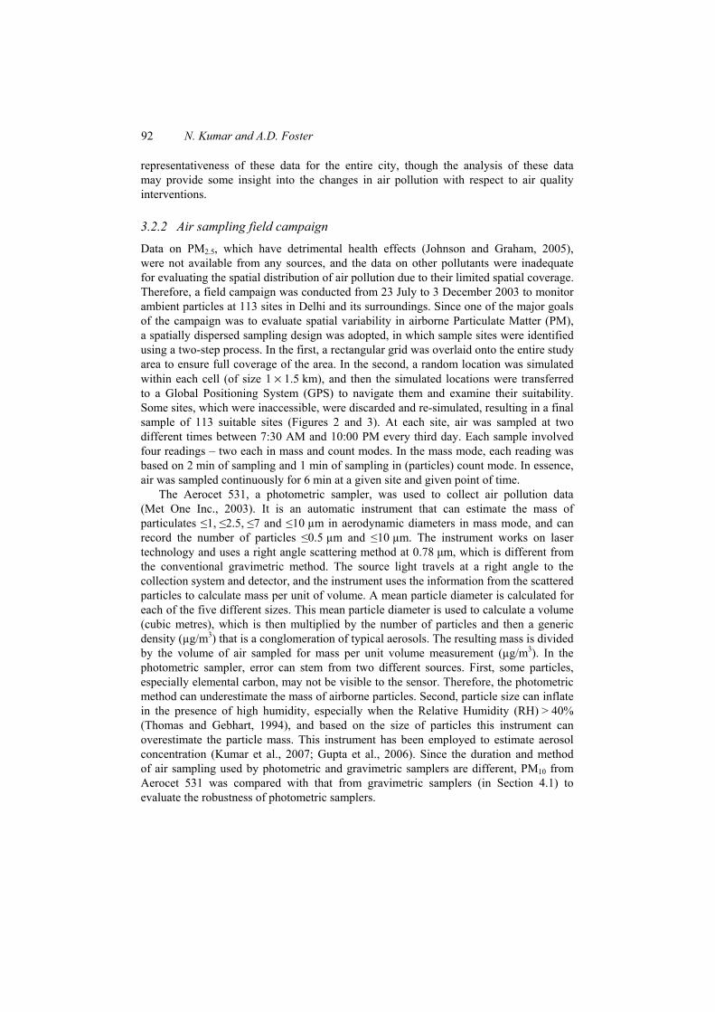
This study focuses on air pollution distribution in Delhi and its surroundings. Delhi and its ten neighbouring districts of three other states form the National Capital Region (NCR), which was enacted to divert the burden of Delhi’s growth in the surrounding areas (Table 1, Figure 1) (DDA, 1996). Delhi is the second largest metropolitan area in India, and its population has increased from 9.4 million in 1991 to 13.2 million in 2001 (at 3.34% annual exponential growth rate) (Census of India, 2001). The number of industrial units in Delhi increased from 8000 in 1951 to 125,000 in 1991, and number of automobiles increased from 235,000 in 1975 to 4,236,675 in 2003–2004 (Government of India, 2006). Prior to the regulations, Delhi was declared to be the 10th most polluted city in the world in terms of airborne SPM (Government of India, 2006). In part, this laid the foundation of recent air quality regulations.

Delhi is an instructive location to study the spatiotemporal distribution of air pollution with reference to a series of rulings by the Indian Supreme Court. Of particular importance was the September 2000 ruling directed at the so-called ‘non-conforming areas’ (TERI, 2001a). These are areas in which most of the industrial activities are supposed to be excluded, but in which industrial growth has continued unabated. The potential impact of these rulings is very large. According to a survey of the Delhi government, 98,000 of the total of 125,000 industries were in non-conforming areas. Subsequent to the decision, 38,000 establishments in sectors with particularly high levels of pollution were subject to this ruling. A large number of industrial plots on the periphery of the city were developed to house roughly 24,000 establishments. While this ruling has been met with substantial resistance and change has proceeded slowly, the ruling remains in force and concerted attempts were made to relocate industries (TERI, 2001b).


Figure 1 National Capital Regions: population density and CNG regulations (see online version for colours)

Table 1 Population growth in national capital region, 1981–1991

1991 1981 Annual exponential

growth rate (%)District/statename Total Rural Urban Total Rural Urban Total Rural Urban

Panipat 677157 467561 209596 492279 340841 151433 3.24 3.21 3.30

Sonipat 754866 576841 178025 593681 467821 125860 2.43 2.12 3.53

Rohtak 1867193 1423133 444060 1516142 1223830 292312 2.10 1.52 4.27

Faridabad 1477240 759727 717513 986076 577446 408630 4.12 2.78 5.79

Gurgaon 1146090 913386 232704 863865 694634 169231 2.87 2.78 3.24

Rewari 623301 528101 95200 496813 437494 59319 2.29 1.90 4.84

Haryana 6545847 4668749 1877098 4948856 3742065 1206786 2.84 2.24 4.52

Alwar 1395513 1115704 279809 1048886 861095 187791 2.90 2.62 4.07


Table 1 Population growth in national capital region, 1981–1991 (continued)

1991 1981 Annual exponential

growth rate (%)District/statename Total Rural Urban Total Rural Urban Total Rural Urban

Rajasthan 1395513 1115704 279809 1048886 861095 187791 2.90 2.62 4.07

Meerut 3447912 2171355 1276557 2767185 1903270 863915 2.22 1.33 3.98

Ghaziabad 2703933 1455673 1248260 1843297 1214180 629117 3.91 1.83 7.09

Bulandshahr 2849859 2257064 592795 2358569 1902422 456147 1.91 1.72 2.65

Uttar Pradesh 9001704 5884092 3117612 6969051 5019871 1949180 2.59 1.60 4.81

Delhi 9420644 949019 8471625 6220300 452216 5768084 4.24 7.69 3.92

Delhi UT 9420644 949019 8471625 6220300 452216 5768084 4.24 7.69 3.92

NCR 26363708 12617564 13746144 19187093 10075247 9111841 3.23 2.28 4.20

Source: Census of India (1981, 1991)

The second Supreme Court ruling mandated the conversion of buses and three-wheelers from gasoline/diesel to CNG in 2000 and 2001. It took the state about two years to implement this ruling, and the final bus registered in Delhi was converted to CNG in December 2002 (Bell et al., 2004). The conversion of a diesel-based engine to CNG was a costly proposition (Rajalakshmi and Venkatesan, 2001). Therefore, most diesel-based commercial vehicles might have been migrated to the neighbouring states, largely unaffected by the CNG regulations. Moreover, it was anticipated that different parts of the region would have been differentially affected by these initiatives, given the differences in levels of traffic through these regions. Though these regulations were expected to reduce the pollution level in Delhi, we expect that the air pollution must have been redistributed, since most polluting vehicles and industries that were subject to these regulations might have migrated to the neighbouring states. Therefore, spatially detailed air pollution data and a cross-sectional comparison of air pollution in Delhi vis-à-vis outside Delhi’s border can provide insight into the effect of these regulations on air pollution redistribution.

3.2 Data

The air pollution data for this research come from two different sources:

• CPCB

• a field campaign from July to December 2003.

3.2.1 Air pollution data from CPCB

Air pollution data for seven major cities were acquired from CPCB to construct the trend of air pollution in Delhi and other cities from 2000 to 2005. Data on sulphur dioxide (SO2), nitrogen dioxide (NO2) and PM10 were collected. The PM10 data are collected in three different shifts 6:00–14:00, 14:00–22:00 and 22:00–6:00 (of the following day) using filter-based high volume samplers. None of the CPCB facilities, however, was equipped to monitor PM2.5. Since the data on these pollutants are monitored continuously at a central location, readers should be cautioned about the


representativeness of these data for the entire city, though the analysis of these data may provide some insight into the changes in air pollution with respect to air quality interventions.

3.2.2 Air sampling field campaign

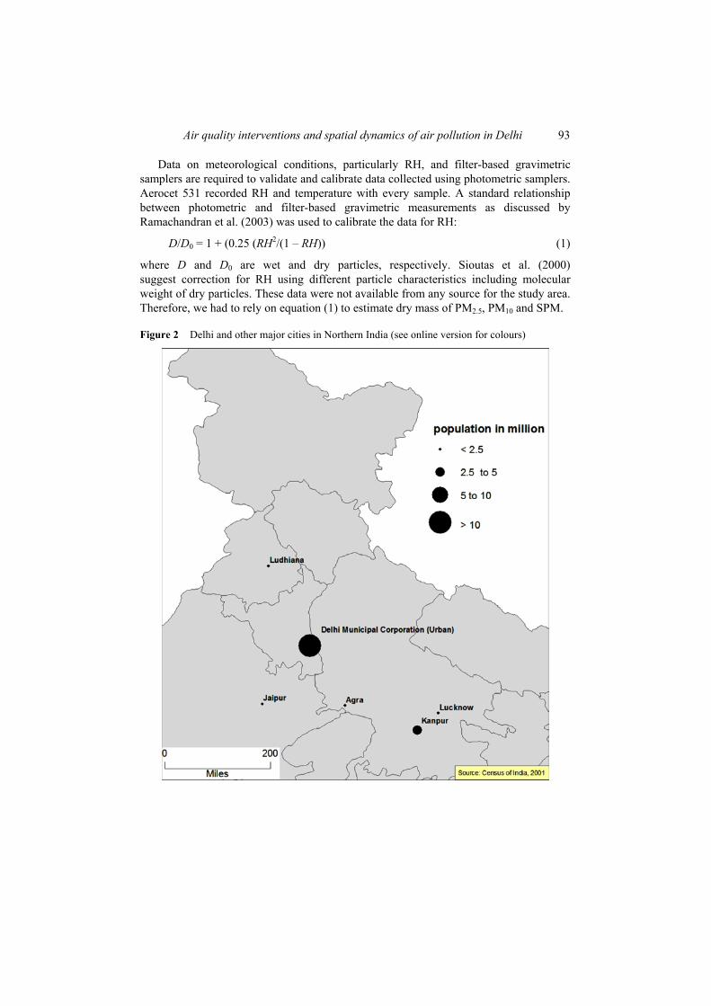
Data on PM2.5, which have detrimental health effects (Johnson and Graham, 2005), were not available from any sources, and the data on other pollutants were inadequate for evaluating the spatial distribution of air pollution due to their limited spatial coverage. Therefore, a field campaign was conducted from 23 July to 3 December 2003 to monitor ambient particles at 113 sites in Delhi and its surroundings. Since one of the major goals of the campaign was to evaluate spatial variability in airborne Particulate Matter (PM), a spatially dispersed sampling design was adopted, in which sample sites were identified using a two-step process. In the first, a rectangular grid was overlaid onto the entire study area to ensure full coverage of the area. In the second, a random location was simulated within each cell (of size 1 × 1.5 km), and then the simulated locations were transferred to a Global Positioning System (GPS) to navigate them and examine their suitability. Some sites, which were inaccessible, were discarded and re-simulated, resulting in a final sample of 113 suitable sites (Figures 2 and 3). At each site, air was sampled at two different times between 7:30 AM and 10:00 PM every third day. Each sample involved four readings – two each in mass and count modes. In the mass mode, each reading was based on 2 min of sampling and 1 min of sampling in (particles) count mode. In essence, air was sampled continuously for 6 min at a given site and given point of time.

The Aerocet 531, a photometric sampler, was used to collect air pollution data (Met One Inc., 2003). It is an automatic instrument that can estimate the mass of particulates 1, 2.5, 7 and 10 µm in aerodynamic diameters in mass mode, and can record the number of particles 0.5 µm and 10 µm. The instrument works on laser technology and uses a right angle scattering method at 0.78 µm, which is different from the conventional gravimetric method. The source light travels at a right angle to the collection system and detector, and the instrument uses the information from the scattered particles to calculate mass per unit of volume. A mean particle diameter is calculated for each of the five different sizes. This mean particle diameter is used to calculate a volume (cubic metres), which is then multiplied by the number of particles and then a generic density (µg/m3) that is a conglomeration of typical aerosols. The resulting mass is divided by the volume of air sampled for mass per unit volume measurement (µg/m3). In the photometric sampler, error can stem from two different sources. First, some particles, especially elemental carbon, may not be visible to the sensor. Therefore, the photometric method can underestimate the mass of airborne particles. Second, particle size can inflate in the presence of high humidity, especially when the Relative Humidity (RH) > 40% (Thomas and Gebhart, 1994), and based on the size of particles this instrument can overestimate the particle mass. This instrument has been employed to estimate aerosol concentration (Kumar et al., 2007; Gupta et al., 2006). Since the duration and method of air sampling used by photometric and gravimetric samplers are different, PM10 from Aerocet 531 was compared with that from gravimetric samplers (in Section 4.1) to evaluate the robustness of photometric samplers.


Data on meteorological conditions, particularly RH, and filter-based gravimetric samplers are required to validate and calibrate data collected using photometric samplers. Aerocet 531 recorded RH and temperature with every sample. A standard relationship between photometric and filter-based gravimetric measurements as discussed by Ramachandran et al. (2003) was used to calibrate the data for RH:

D/D0 = 1 + (0.25 (RH2/(1 – RH)) (1)

where D and D0 are wet and dry particles, respectively. Sioutas et al. (2000) suggest correction for RH using different particle characteristics including molecular weight of dry particles. These data were not available from any source for the study area. Therefore, we had to rely on equation (1) to estimate dry mass of PM2.5, PM10 and SPM.

Figure 2 Delhi and other major cities in Northern India (see online version for colours)


Figure 3 Air pollution monitoring sites and sources of air pollution in Delhi and its surroundings (see online version for colours)

3.2.3 Data on the source of air pollution

This paper focuses on two main sources of air pollutants, namely traffic and industries. Data for traffic were collected along with the air pollution data. Number of vehicles were counted during each sample and then classified by type – heavy vehicles (including buses and trucks), cars, three-wheelers and others. Data on industrial clusters were generated from the Eicher Map of Delhi (EICHER, 2001), in which land-use and land-cover were largely based on the Survey of India’s large-scale topographic maps.

3.3 Methods

Our analysis is based on three different methods:

• proximity analysis for data integration

• spatial interpolation of air pollution surfaces

• regression modelling

which are discussed below.

3.3.1 Data processing

As mentioned earlier, data were collected at each site at two different times every third day. On an average, we have more than 65 samples at each site, which adequately


represent air quality at different times of a day and different days of a week. Each sample included two readings (the first 4 min of sampling in the mass mode). The data used in the analysis are the averages over 23 July through 3 December 2003. The frequency of vehicles is the average number of vehicles (by their types) every 1 min for the same period. Proximity to road and industrial cluster were computed using spatial join in ArcGIS Ver 9.x (ESRI, 2005), which computed the Cartesian distance of all sample sites to their closest sources (road and industrial clusters in our case).

3.3.2 Spatial interpolation

Various methods of interpolation are available to compute continuous surface. We employed Kriging, which estimates air pollution at a given pixel as an inverse function of distance weighted by spatial autocorrelation among the sample sites (Cressie, 1990; Isaaks and Srivastava, 1989), to interpolate surfaces of PM2.5, PM10 and SPM. Kriging uses a semivariogram, developed from the spatial structure in the data, to determine the weight. Another advantage of Kriging is that it yields a set of spatial predictions at sampled locations and also provides an associated variance that measures the uncertainty in the predictions. The optimal parameters, such as distance range, distance exponent, were computed by minimising variance between actual and estimated values at the sample sites (Table 2):

2 2( ) ( )

1

1min | | ( )ˆn

si sisi

zznσ

=

= −ä (1)

wheren: number of sample sites

( )ˆ siz : estimated value at site (si)z(si): observed value at site (si).

Table 2 Parameters used for kriging to create air pollution surface

Parameter Value Semivariogram model Exponential Anisotropic direction 306 Major range (DD) 0.39 Minor range (DD) 0.18 Lag size (degree decimals) 0.033 No. of points included 12 Neighbours to include 15 or at least 10 for each angular sector Angular sector 4

The sill and nugget were computed using the automatic function within ArcMap to obtain the best fit for the semivariogram.


3.3.3 Air pollution and its sources: regression model

Two different sets of regression models were employed to examine the contribution of different sources (of air pollution) on the levels of air pollution observed at a sample site. In the first set, air pollution at a sample site (si) was modelled as a function of the selected covariates X(si), which included proximity to the major roads, industrial clusters, frequency of buses and other heavy vehicles per minute, using an Ordinary Least Square (OLS) regression model:

(si) ( ) ( )= + +si sia Xτ β ε′ (2)

where β is a vector of regression coefficients, and

( ) = unobservablesiε .

In the second set, Spatial Autoregressive Models (SAM) were used because the error term (ε) observed a statistically significant spatial autocorrelation, which cannot be handled by the OLS models as the one of the main assumptions of the OLS is that ε ~ N (0, σ2). Three different models, namely Conditional Autoregressive (CAR), Simultaneous Autoregressive (SAR) and SAM, were considered. In the first, the spatial dependence in the residuals is expected to have a conditional distribution, and joint distribution in the second. In the third (i.e., SAM), we could represent the residuals that are not explained in the OLS with a variable R(si), which can be composed of distance-weighted residuals of neighbours from the OLS model as in equation (1). This way, we would no longer need to assume dependency for the outcome variable. One of the advantages of this approach is that it is easily understandable. Another advantage is that we could avoid the problem of counterintuitive results in SAR and CAR as demonstrated by Wall (2004).

More formally, assuming that the response variable is normally distributed, we could define the model as follows:

( ) ( ) ( ) ( )= + +si si si sia X Rτ β ρ ε′ + (3)

where

R(si): information not explained in the OLS : parameter coefficients

ε ~ N(0, σ2) iid.

There are various ways to estimate R(si). Institutively, R(si) can be estimated as an inverse distance weighted average of residuals at the neighbouring sites ( j), as

( ) ( ) ( )( )( ) 1( )( )( ) 1

1 k

si sj si sjksjsi sjsj

R dd

ωω

τ −

−=

=

= ää

(4)

where

τ (sj): residual at neighbouring site (sj)k: number of neighbouring sites


dij: distance between site si and neighbouring sj, and dij < hh: distance range ω: distance exponent.

The distance range (h) and distance exponent (ω) were estimated with the aid of empirical semivariogram. The distance range refers to the distance threshold where the semivariogram levels off to nearly a constant value, called as the sill, and the shape of semivariogram can help us determine the distance exponent. For PM2.5 and PM10,distance ranges were 4.5 and 3.0 km, respectively, and distance exponent for both was −2, which means that the nearer neighbours were weighted heavily than the distant neighbours.

4 Analysis

4.1 Data validation: photometric and gravimetric measurements

Generally, high volume samplers are used to monitor ambient particles. The field campaign data, however, were collected using photometric samplers, which work on the laser technology and can monitor particles in real time. Gravimetric samplers, however, require a minimum of 8 h of sampling. Filters are weighed before and after the sampling, and based on the mass gained during the sampling period and the amount of air sampled, mass density (µg/m3) is computed. Given the cost of gravimetric samplers, it was not plausible to deploy these samplers at a large number of locations. Therefore, real-time photometric samplers were used to monitor air quality at relatively large number of locations n ~ 113. To assess the robustness of photometric samplers, estimates from these samplers were compared against those from gravimetric samplers at one site in Delhi located near the Income Tax Office (ITO), which is operational continuously.

During August to November 2003, the daily averages of PM10 from CPCB site and our instrument were 203 ± 26.8 µg/m3 and 153 ± 33.5 µg/m3, respectively. The photometric estimates were significantly lower than the gravimetric estimates. Given the differences in the method of operation and duration of sampling by gravimetric (24 h average) and real-time photometric measurements (6 min for each sample), a difference of 49.5 ± 31 µg/m3 (95% CI) seems reasonable. In addition, the regression analysis suggests a statistically significant positive association in the temporal variability in PM10 measured by both methods (Figure 4). It was not possible to validate PM2.5because of the non-availability of PM2.5 data from gravimetric samplers. Based on other research, however, the difference between photometric and gravimetric estimates is expected to be smaller for PM2.5 than for PM10 (Ramachandran et al., 2003). Using the empirical relationship RH and particle size developed by Thomas and Gebhart (1994), photometric estimates can be calibrated to gravimetric standards (Ramachandran et al., 2003).


Figure 4 PM10 (µg/m3) from photometric and gravimetric samplers at ITO, Delhi,23 July–December 2003 (see online version for colours)

4.2 Descriptive analysis

The levels of PM2.5 and PM10 in the study area were significantly higher than the standards recommended by CPCB, the Environmental Protection Agency (EPA) of the USA and WHO. According to EPA, the three-year average of PM2.5 should be

15 µg/m3. The average value of PM2.5 in Delhi over a five-month period was recorded as 28.2 ± 1.8 µg/m3 (95% CI), and PM10 and SPM averages were 157 ± 18.1 µg/m3

and 189 ± 21.8 µg/m3, respectively (Tables 3 and 4). The summary statistics of the different sources of air pollutants is presented in Table 4. Among automobiles, cars and non-CNG heavy vehicles recorded the highest (18.9 ± 3.5) and the lowest frequency (1.8 ± 0.2), respectively; the average distance to the closest industrial cluster was 2.4 ± 0.37 km.

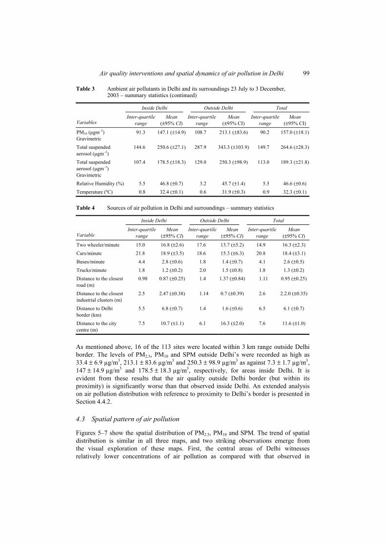
Table 3 Ambient air pollutants in Delhi and its surroundings 23 July to 3 December, 2003 – summary statistics

Inside Delhi Outside Delhi Total

Variables Inter-quartile

rangeMean

(±95% CI)Inter-quartile

rangeMean

(±95% CI) Inter-quartile

rangeMean

(±95% CI)

PM2.5 (µgm–3)Aerosol

11.9 39.1 (±2.3) 21.2 46.7 (±7.1) 14.0 40.2 (±2.3)

PM2.5 (µgm–3)Gravimetric

8.5 27.3(±1.7) 14.9 33.4 (±6.9) 8.8 28.2 (±1.8)

PM7 (µgm–3)Aerosol

91.7 172.9 (±18.0) 210.7 241.1 (±66.7) 94.7 183.1 (±18.7)

PM7 (µgm–3)Gravimetric

67.7 120.4 (±11.8) 82.8 173.1 (±63.3) 67.9 128.3 (±14.1)

PM10 (µgm–3)Aerosol

113.8 207.1 (±22.2) 254.7 291.9 (±86.3) 125.8 219.9 (±23.4)


Table 3 Ambient air pollutants in Delhi and its surroundings 23 July to 3 December, 2003 – summary statistics (continued)


Variables Inter-quartile

rangeMean


rangeMean

(±95% CI) Inter-quartile

rangeMean

(±95% CI)

PM10 (µgm–3)Gravimetric

91.3 147.1 (±14.9) 108.7 213.1 (±83.6) 90.2 157.0 (±18.1)

Total suspended aerosol (µgm–3)

144.6 250.6 (±27.1) 287.9 343.3 (±103.9) 149.7 264.6 (±28.3)

Total suspended aerosol (µgm–3)Gravimetric

107.4 178.5 (±18.3) 129.0 250.3 (±98.9) 113.0 189.3 (±21.8)

Relative Humidity (%) 5.5 46.8 (±0.7) 3.2 45.7 (±1.4) 5.5 46.6 (±0.6) Temperature (ºC) 0.8 32.4 (±0.1) 0.6 31.9 (±0.3) 0.9 32.3 (±0.1)

Table 4 Sources of air pollution in Delhi and surroundings – summary statistics


Variable Inter-quartile

rangeMean


rangeMean


rangeMean

(±95% CI)

Two wheeler/minute 15.0 16.8 (±2.6) 17.6 13.7 (±5.2) 14.9 16.3 (±2.3) Cars/minute 21.8 18.9 (±3.5) 18.6 15.3 (±6.3) 20.8 18.4 (±3.1) Buses/minute 4.4 2.8 (±0.6) 1.8 1.4 (±0.7) 4.1 2.6 (±0.5) Trucks/minute 1.8 1.2 (±0.2) 2.0 1.5 (±0.8) 1.8 1.3 (±0.2) Distance to the closest road (m)

0.98 0.87 (±0.25) 1.4 1.37 (±0.84) 1.11 0.95 (±0.25)

Distance to the closest industrial clusters (m)

2.5 2.47 (±0.38) 1.14 0.7 (±0.39) 2.6 2.2.0 (±0.35)

Distance to Delhi border (km)

5.5 6.8 (±0.7) 1.4 1.6 (±0.6) 6.5 6.1 (±0.7)

Distance to the city centre (m)

7.5 10.7 (±1.1) 6.1 16.3 (±2.0) 7.6 11.6 (±1.0)

As mentioned above, 16 of the 113 sites were located within 3 km range outside Delhi border. The levels of PM2.5, PM10 and SPM outside Delhi’s were recorded as high as 33.4 ± 6.9 µg/m3, 213.1 ± 83.6 µg/m3 and 250.3 ± 98.9 µg/m3 as against 7.3 ± 1.7 µg/m3,147 ± 14.9 µg/m3 and 178.5 ± 18.3 µg/m3, respectively, for areas inside Delhi. It is evident from these results that the air quality outside Delhi border (but within its proximity) is significantly worse than that observed inside Delhi. An extended analysis on air pollution distribution with reference to proximity to Delhi’s border is presented in Section 4.4.2.

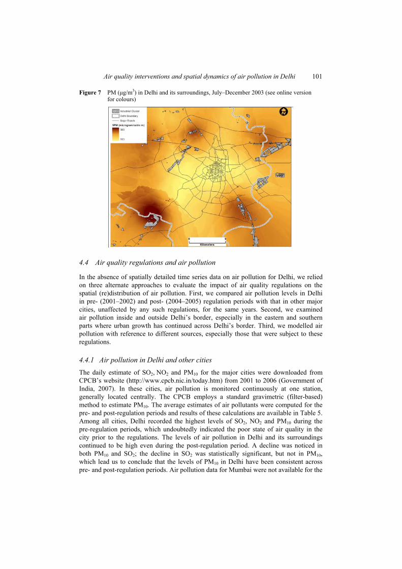
4.3 Spatial pattern of air pollution

Figures 5–7 show the spatial distribution of PM2.5, PM10 and SPM. The trend of spatial distribution is similar in all three maps, and two striking observations emerge from the visual exploration of these maps. First, the central areas of Delhi witnesses relatively lower concentrations of air pollution as compared with that observed in


the peripheral areas, albeit the minimum concentration of PM2.5, PM10 and SPM inside and outside Delhi being much higher than the WHO standards. The elevated levels of air pollution in the areas outside Delhi’s border could be because of the absence of air quality regulations and in-migration of polluting industries and vehicles in these areas. Second, among industrial areas, Ashok Vihar, Sahibabad, Okhla and industrial areas surrounding Delhi–Gurgaon border (around the intersection of National Highway 8 with Delhi border) recorded high levels of the selected pollutants, which indicates that industries are likely to be an important source of PM2.5, PM10 and SPM.

Figure 5 PM2.5 (µg/m3) in Delhi and its surroundings, July–December 2003 (see online version for colours)

Figure 6 PM10 (µg/m3) in Delhi and its surroundings, July–December 2003 (see online version for colours)


Figure 7 PM (µg/m3) in Delhi and its surroundings, July–December 2003 (see online version for colours)

4.4 Air quality regulations and air pollution

In the absence of spatially detailed time series data on air pollution for Delhi, we relied on three alternate approaches to evaluate the impact of air quality regulations on the spatial (re)distribution of air pollution. First, we compared air pollution levels in Delhi in pre- (2001–2002) and post- (2004–2005) regulation periods with that in other major cities, unaffected by any such regulations, for the same years. Second, we examined air pollution inside and outside Delhi’s border, especially in the eastern and southern parts where urban growth has continued across Delhi’s border. Third, we modelled air pollution with reference to different sources, especially those that were subject to these regulations.

4.4.1 Air pollution in Delhi and other cities

The daily estimate of SO2, NO2 and PM10 for the major cities were downloaded from CPCB’s website (http://www.cpcb.nic.in/today.htm) from 2001 to 2006 (Government of India, 2007). In these cities, air pollution is monitored continuously at one station, generally located centrally. The CPCB employs a standard gravimetric (filter-based) method to estimate PM10. The average estimates of air pollutants were computed for the pre- and post-regulation periods and results of these calculations are available in Table 5. Among all cities, Delhi recorded the highest levels of SO2, NO2 and PM10 during the pre-regulation periods, which undoubtedly indicated the poor state of air quality in the city prior to the regulations. The levels of air pollution in Delhi and its surroundings continued to be high even during the post-regulation period. A decline was noticed in both PM10 and SO2; the decline in SO2 was statistically significant, but not in PM10,which lead us to conclude that the levels of PM10 in Delhi have been consistent across pre- and post-regulation periods. Air pollution data for Mumbai were not available for the


year 2001–2002, but during the year 2004–2005 Mumbai, the most populous city in India (Census of India, 2001), witnessed the worst air quality in terms of three air pollutants – PM10, SO2, and NO2 (Table 5).

Table 5 Ambient air pollutants in Delhi and other major cities 2001–2002 and 2004–2005 (µgm–3 (95% CI))


A comparison of the trend of air pollution in Delhi with that in Kanpur can be particularly useful to assess the impact of air quality regulations in Delhi, because Kanpur and Delhi are situated in identical topographic and climatic conditions, and Kanpur is the largest city closest to Delhi (Census of India, 2001), and was not subject to any regulations. The average PM10 in Delhi declined slightly from 240.2 ± 22.7 µg/m3 in 2001–2002 to 239.8 ± 10.9 µg/m3 2004–2005. In Kanpur, however, the PM10 increased from 178.5 ± 12.8 µg/m3 in 2001–2002 to 198.3 ± 15.3 µg/m3 in 2004–2005, a net increase of about 20.42 µg/m3 over a span of just four years. This clearly indicates that the enforcement of environmental regulations in Delhi have been working to stabilise the levels of air pollution. In Kanpur, however, the air quality has deteriorated significantly over a span of four years and this deterioration can be attributed to the absence of air quality regulations similar to what were imposed on Delhi.

Interpretation of these results should be used with caution, because PM10 is not a robust indicator of air quality in a semi-dry climate where dust is a major contributor of PM10 mass (Kumar et al., 2007). Data on PM2.5 are not available for any of the cities. Therefore, using a cross-sectional approach, a comparison of PM2.5 mass (and other pollutant) inside and outside Delhi will be used to evaluate the impact of these regulations on air pollution redistribution.

4.4.2 Air pollution inside and outside Delhi border

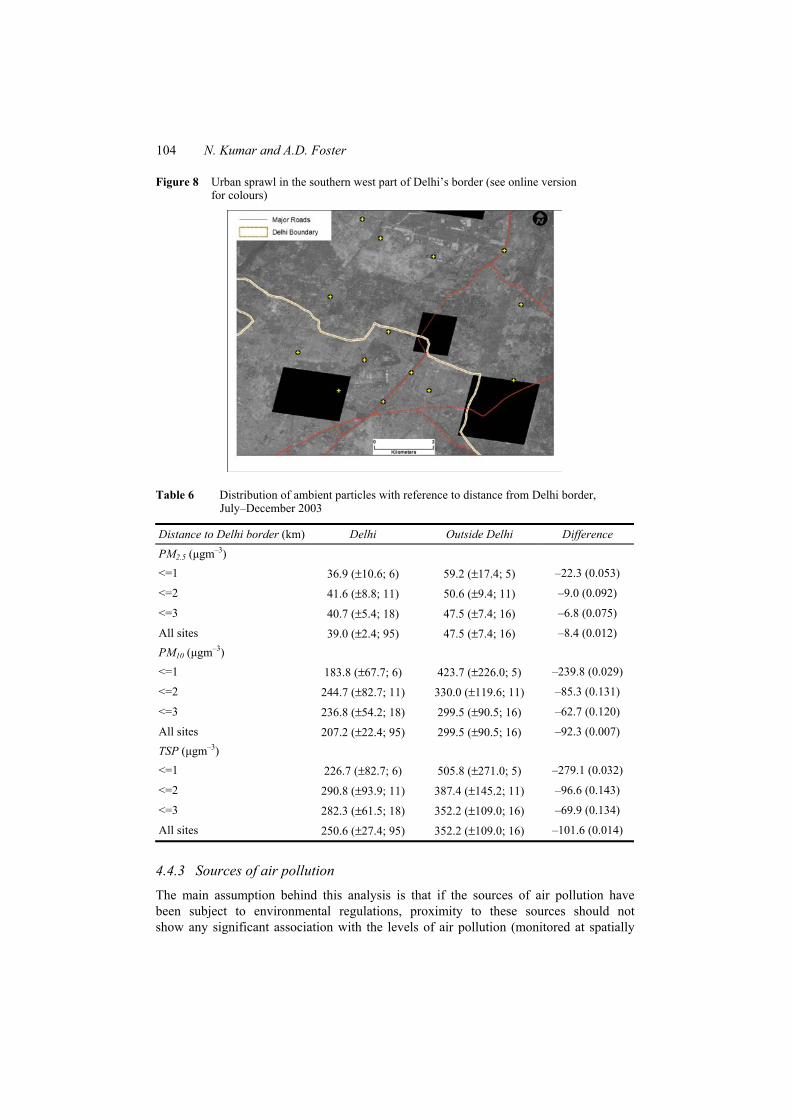
As is evident from Section 4.2, bordering areas (both inside and outside) Delhi recorded relatively high levels of PM2.5 and PM10. In this section, air pollutant is examined inside and outside Delhi border at different distance intervals. This can allow us to evaluate the effect of recent environmental regulations on air pollution redistribution. The main assumption behind the analysis, however, is that the air quality of areas bordering Delhi (both inside and outside) was same prior to the regulations, because urban growth has spread across Delhi’s border in eastern, south eastern and southern parts (Figure 8), and functional characteristics of these areas were expected to the same. Therefore, prior to the regulations, the sources and levels of air pollution should have been the same in these areas. Based on this assumption, we hypothesise that the differences in air pollution levels inside and outside short distances ( 2 km) can be attributed to air quality regulations.

The analysis of our data suggests that the levels of air pollution within 2 km outside Delhi’s border were significantly higher than the areas inside 2 km of Delhi’s border, and the ratio of outside to inside air pollution declines with distance from the border in both directions (Table 6). This proves our hypothesis and demonstrates the differential impact of regulations inside and outside Delhi border. While the regulations, namely conversion of buses to CNG and closure of polluting industries, were expected to improve the air quality in Delhi, these regulations seemed to have adversely impacted the air quality of areas outside Delhi border, because these areas are suspected to have attracted a large number of polluting industries and vehicles that were subject to the regulations. From our analysis, it is evident that the air quality of these areas is very likely to deteriorate further in the absence of air quality regulations.


Figure 8 Urban sprawl in the southern west part of Delhi’s border (see online versionfor colours)

Table 6 Distribution of ambient particles with reference to distance from Delhi border,July–December 2003

Distance to Delhi border (km) Delhi Outside Delhi Difference PM2.5 (µgm–3) <=1 36.9 (±10.6; 6) 59.2 (±17.4; 5) –22.3 (0.053)

<=2 41.6 (±8.8; 11) 50.6 (±9.4; 11) –9.0 (0.092)

<=3 40.7 (±5.4; 18) 47.5 (±7.4; 16) –6.8 (0.075)

All sites 39.0 (±2.4; 95) 47.5 (±7.4; 16) –8.4 (0.012) PM10 (µgm–3) <=1 183.8 (±67.7; 6) 423.7 (±226.0; 5) –239.8 (0.029)

<=2 244.7 (±82.7; 11) 330.0 (±119.6; 11) –85.3 (0.131)

<=3 236.8 (±54.2; 18) 299.5 (±90.5; 16) –62.7 (0.120)

All sites 207.2 (±22.4; 95) 299.5 (±90.5; 16) –92.3 (0.007) TSP (µgm–3) <=1 226.7 (±82.7; 6) 505.8 (±271.0; 5) –279.1 (0.032)

<=2 290.8 (±93.9; 11) 387.4 (±145.2; 11) –96.6 (0.143)

<=3 282.3 (±61.5; 18) 352.2 (±109.0; 16) –69.9 (0.134)

All sites 250.6 (±27.4; 95) 352.2 (±109.0; 16) –101.6 (0.014)

4.4.3 Sources of air pollution

The main assumption behind this analysis is that if the sources of air pollution have been subject to environmental regulations, proximity to these sources should not show any significant association with the levels of air pollution (monitored at spatially


dispersed sites). In the study area, there are three main sources of air pollution, namely industries (including three thermal plants), automobiles and cooking (Government of India, 2006; Elsom and Longhurst, 2004). Among these, only diesel buses and autorickshaws were converted to CNG and a limited number of polluting industries faced closure. To examine the impact of these interventions, spatial distribution of air pollution was examined with respect to sources of air pollution, namely frequency of different types of vehicles (particularly buses and trucks) and proximity to industrial clusters. Two different set models were examined:

• in the first set, the impact of air pollution sources was examined on PM2.5 and PM10inside and outside Delhi (Tables 7 and 8)

• in the second, PM2.5 and PM10 were regressed on the selected sources of air pollution using OLS regression model and spatial autoregressive model (Table 9).

As hypothesised, the frequency of buses, which were converted to CNG (during 2001–2002) observed an insignificant association with PM2.5 and PM10, particularly inside Delhi. In contrast, the frequency of non-CNG heavy vehicles emerged as the most important predictor of both PM2.5 and PM10 (Figure 9(a) and (b)); it explains 21% and 12% of the total variability in PM2.5 and PM10, respectively (Table 7). Among other sources, proximity to industrial clusters, measured by Cartesian distance, emerged as the second most important predictor of PM2.5 and PM10 (Figure 9(c) and (d)) and proximity to road shows a significant positive association with PM10, but its association with PM2.5was statistically insignificant. This means that dust could be one of the major constituents of PM10. The results of our analysis support that the combustion from the heavy vehicles (except CNG buses) and industries were two major contributors of PM2.5 in the post-regulation period (Nagendra and Khare, 2003). These two sources together explain about one-third of the total variability in PM2.5 (Table 9).

Table 7 Log(PM2.5) and pollution sources

(Trucks/minute)^0.5 (Buses/minute)^0.5 (Cars/Minute)^0.5

Distance to the closest industrial

cluster (km) Distance to the

closest road (km)

Covariates Model 1 Model 2 Model 1 Model 2 Model 1 Model 2 Model 1 Model 2 Model 1 Model 2

0.166 0.162 0.036 0.048 0.014 0.016 –0.004 –0.003 0.002 0.002 Pollutionsource (4.47)** (4.48)** –1.400 –1.900 –1.100 –1.310 (3.65)** (2.80)** –1.620 –1.420

0.166 0.197 0.183 0.1 0.168 OutsideDelhi = 1 (2.73)** (3.00)** (2.79)** –1.44 (2.57)*

3.49 3.469 3.599 3.553 3.593 3.557 3.802 3.761 3.598 3.579 Constant

(84.3)** (84.7)** (86.8)** (83.0)** (66.9)** (66.2)** (78.2)** (66.7)** (93.9)** (94.0)**

Obs. 112 112 112 112 112 112 112 112 112 112

R-squared 0.15 0.21 0.02 0.09 0.01 0.08 0.11 0.12 0.02 0.08

Absolute value of t statistics in parentheses. *Significant at 5%. **Significant at 1%.


Table 8 Log(PM10) and pollution sources

(Trucks/minute)^0.5 (Buses/minute)^0.5 (Cars/minute)^0.5

Distance to the closest industrial

cluster (km)Distance to the

closest road (km)

Covariates Model 1 Model 2 Model 1 Model 2 Model 1 Model 2 Model 1 Model 2 Model 1 Model 2

0.201 0.194 –0.015 0.004 –0.017 –0.013 –0.007 –0.006 0.005 0.004 Pollutionsource (2.90)** (2.86)** (0.31) (0.08) (0.75) (0.60) (3.86)** (3.07)** (2.17)* (1.98)

0.29 0.30 0.30 0.15 0.28 OutsideDelhi = 1 (2.52)* (2.53)* (2.51)* (1.22) (2.40)*

5.07 5.03 5.28 5.21 5.32 5.26 5.55 5.49 5.14 5.11 Constant

(65.4)** (65.3)** (70.6)** (66.8)** (55.3)** (54.3)** (64.3)** (54.6)** (75.8)** (75.5)**

Obs. 112.00 112.00 112.00 112.00 112.00 112.00 112.00 112.00 112.00 112.00

R-squared 0.07 0.12 0.00 0.06 0.01 0.06 0.12 0.13 0.04 0.09


Table 9 Ambient particles and sources of air pollution – OLS and Spatial Autoregressive Models

Log(PM2.5) Log(PM10)

OLS SAM OLS SAM 0.258 0.261 0.477 0.46 (Trucks/minute)^0.5

(3.66)** (3.71)** (3.82)** (3.76)** –0.002 –0.002 –0.003 –0.004 SQRT(Distance to Industrial Cluster (m))(1.53) (1.62) (1.46) (1.77) 0.002 0.002 0.003 0.003 SQRT(Distance to the major road) (1.52) (1.46) (1.51) (1.37) –0.067 –0.068 –0.215 –0.203 SQRT(Buses/minute)(1.46) (1.48 (2.63)** (2.55)* 0.079 0.086 0.09 0.102 Outside Delhi Border = 1 (1.14) (1.25) (0.73) (0.85)

0.24 0.385 Spatial autocorrelation (1.31) (2.46)*

3.52 3.523 5.14 5.172 Constant(40.25)** (40.41)** (33.13)** (34.01)**

Observations 111 111 111 111 R-squared 0.3 0.31 0.28 0.32



Figure 9 Air pollution and its sources: (a) PM2.5 and frequency of non-CNG heavy vehicle; (b) PM10 and frequency of non-CNG heavy vehicle; (c) PM2.5 and proximity (distance) to industries and (d) PM10 and proximity to industriesTable-1: population growth in National Capital Region, 1981–1991 (see online version for colours)

(a) (b)

(c) (d)

It is interesting to note that the regression coefficient of the frequency of non-CNG heavy vehicles is stronger outside Delhi when compared with that inside Delhi (Tables 7 and 8). The impact of proximity to industrial cluster on PM2.5 and PM10,however, was stronger inside Delhi. The frequency of buses did not register a significant association with PM2.5, but showed a significant negative association with PM10 inside Delhi and a positive association with PM10 outside Delhi, because buses not registered in Delhi were not subject to CNG regulations, and hence these buses in the areas outside Delhi were diesel-based and hence could be an important contributor of PM2.5.

Our analysis further suggests that the sources that were subject to CNG regulations have done their job, but non-CNG heavy vehicles, industries and addition of a large number of private vehicles (cars) continue to be the major sources of PM2.5 in the study area. Another important thing that emerges from our analysis is that PM10 shows a statistically significant spatial autocorrelation, because coarse particles settle by gravity as distance increases and fine particles stay aloft longer distances and for longer duration.


5 Results and conclusions

From the air quality interventions in Delhi, we can learn a number of lessons. First, these regulations clearly indicate how an independent judicial branch in a democratic society can enact environmental laws, generally reserved to legislators and specialised regulatory bodies of the executive branch, and direct the executive branch to enforce these regulations when political will fails to do so (Bell et al., 2004). Second, until recently it was believed that EKC, which maps the course of environmental pollution as an inverted U-shape function of economic growth, was applicable to western countries (Krupitsky et al., 2005; Stern, 2004). Developing countries, however, have begun to address environment pollution in recent years (Dasgupta et al., 2002). Delhi, which has enforced two major environmental regulations in recent years, is an example of these attempts. The similar CNG regulations are being enforced in Lahore, Pakistan (The Hindustan Times, 2004). These interventions are expected to reverse the increasing trend of air pollution in the City, and its entry in the second phase of EKC, in which air pollution declines, to a certain level, with the positive economic growth. Although the validity of EKC in terms of econometric precision in air pollution–economic growth association is questioned (Stern, 2004), the general idea behind it is still relevant for both developed and developing countries. Now the question before us is to investigate whether the EKC will follow the same course of air pollution (in relation to economic growth) as it did in developed countries. Although this topic is beyond the scope of this research, it will be useful to pursue the application of EKC in Delhi for future research.

Recent air quality interventions were expected to improve air quality in Delhi. But the analysis of our data does not support a significant improvement in air quality in terms of the levels of PM2.5 and PM10 within Delhi, which is consistent with the results reported in Narain and Krupnick (2007). Our analysis further reveals substantial spatial variations in air pollution inside and outside Delhi border. Air quality interventions are most likely to have two major impacts on air pollution (re)distribution inside and outside Delhi. First, closure of H-Class industries – hazardous, noxious, heavy and large polluting – in non-conforming areas resulted in either their relocation to newly developed industrial estates, namely Bawana Industrial Estate in North and Kanjawala in North-West or their migration to the neighbouring states, which were not subject to these regulations. As a result, air quality at the destinations of these polluting industries (whether within the regularised industrial estates in Delhi or outside Delhi) has been adversely affected.

Second, most non-CNG buses that were subject to the regulations are suspected to have moved to the neighbouring states. Therefore, the areas surrounding Delhi have served as a magnet to attract polluting industries and vehicles in the absence of air quality regulations, which could be responsible for high levels of PM2.5, PM10 and SPM in the areas outside Delhi. Polluting industries, particularly, prefer proximity to the city and less stringent environmental regulations. A cross-sectional analysis of data indicates that the elevated levels of PM2.5, PM10 and SPM in the areas outside Delhi could be the result of differential impact of these regulations inside and outside Delhi. Although air pollution levels in most parts of Delhi and its surroundings were significantly higher than the standards recommended by WHO, EPA and CPCB, areas nearing Delhi’s border (±2 km) witnessed significantly higher levels of PM2.5, PM10 and SMP when compared with those observed in the central parts of the study area.


Two important findings emerge from this paper. First, the conversion of buses to CNG seems to be working, as the frequency of buses does not show any significant association with PM2.5 or PM10, particularly inside Delhi. Second, non-CNG heavy vehicles and industries appear to be significant contributors of ambient air pollution, particularly that of PM2.5, product of combustion in urban areas. The proximity to industries and frequency of non-CNG heavy vehicles together accounted for one-third of the total variability in PM2.5. It seems that land-zoning and CNG regulations on commercial vehicles except buses and autorickshaws were not enforced vigorously. In addition, a large number of private vehicles (including diesel cars) are being added every year (Waldman, 2005). Therefore, emission reduced by the CNG regulations could have been offset by the addition of new vehicles (Narain and Krupnick, 2007) and unchecked emission from industries and non-CNG heavy vehicles.

While stringent regulations are required to check air pollution from industries, non-CNG heavy vehicles and private vehicles (such as cars) within the city, areas surrounding Delhi also need to enforce the similar regulations vigorously; otherwise, unabated increase in air pollution in these areas is likely to have severe health consequences. In addition, there is also a need for spatially detailed longitudinal data for effective air quality monitoring and management, because the limited sites in Delhi alone are not sufficient to estimate spatially detailed air pollution surfaces and air quality surveillance. The use of real-time photometric samplers and satellite remote sensing are two substitutes for collecting spatially detailed time-series data (Kumar et al., 2007), which are critically important for computing exposure in micro-environments to study the health effects of air pollution.

Acknowledgements

The Population Studies and Training Center, Brown University and NICHD/NIH (Grant No. R21 HD046571-01A1) supported this research. The authors thank Vineet Kumar, O.P. Malik and Amit Kumar for air pollution and vehicle data collection and O.P. Sharma, IIT Delhi, for his valuable comments and extending access to his laboratory and providing logistic support. Comments and suggestions from Mukesh Khare, Allen Chu, S.N. Tripathi and the anonymous referees are acknowledged with thanks.

ReferencesBell, R.G., Mathur, K., Narain, U. and Simpson, D. (2004) ‘Clearing the air: How Delhi broke the

logjam on air quality reforms’, Environment Magazine, Vol. 46, pp.22–39. Carmichael, G.R., Tang, Y., Kurata, G., Uno, I., Streets, D.G., Thongboonchoo, N., Woo, J.H.,

Guttikunda, S., White, A., Wang, T., Blake, D.R., Atlas, E., Fried, A., Potter, B., Avery, M.A., Sachse, G.W., Sandholm, S.T., Kondo, Y., Talbot, R.W., Bandy, A., Thorton, D. and Clarke, A.D. (2003) ‘Evaluating regional emission estimates using the trace-P observations’, Journal of Geophysical Research-Atmospheres, p.108.

Census of India (2001) Primary Census Abstract, Office of the Registrar General and Census Commissioner of India, Government of India.

Cressie, N. (1990) ‘The origins of kriging’, Mathematical Geology, Vol. 2, pp.239–252.


CSE (2006) The Leapfrog Factor: Clearing the Air in Asian Cities, Centre for Science and Environment, New Delhi.

Dasgupta, S., Laplante, B., Wang, H. and Wheeler, D. (2002) ‘Confronting the environmental Kuznets curve’, Journal of Economic Perspectives, Vol. 16, pp.147–168.

Davidson, C.I., Phalen, R. and Solomon, P. (2005) ‘Airborne particulate matter and human health: a review’, Aerosol Science And Technology, Vol. 39, pp.737–749.

DDA (1996) Master Plan for Delhi: Perspective 2001, T.N.C.T.O.D. (Ed.), Delhi Development Authority, DDA, Delhi.

Dominici, F., Mcdermott, A., Zeger, S.L. and Samet, J.M. (2003) ‘Airborne particulate matter and mortality: timescale effects in four US cities’, American Journal of Epidemiology, Vol. 157, pp.1055–1065.

EICHER (2001) Delhi: City Map, Eicher Goodearth Ltd., New Delhi. Elsom, D.M.M. and Longhurst, J.W.S. (2004) Sectoral Analysis of Air Pollution Control in Delhi,

Wit Press, Billerica, MA. ESRI (2005) Arcgis, Version 9.1, Redlands, CA, Environmental Systems Research Institute. Government of India (2006) White Paper on Pollution in Delhi with an Action Plan, Ministry of

Environment and Forests, New Delhi. Government of India (2007) Air Quality in Major Cities, Board, C.P.C. (Ed.), Government of India. Gupta, P., Christopher, S.A., Wang, J., Gehrig, R., Lee, Y.C. and Kumar, N. (2006)

‘Satellite remote sensing of particulate matter and air quality assessment over global cities’, Atmospheric Environment, Vol. 40, No. 30, pp.5880–5892.

Isaaks, E.H. and Srivastava, R.M. (1989) An Introduction To Applied Geostatistics, Oxford University Press, New York.

Johnson, P.R. and Graham, J.J. (2005) ‘Fine particulate matter national ambient air quality standards: public health impact on populations in the Northeastern United States’, Environ.Health Perspect., Vol. 113, pp.1140–1147.

Kathuria, V. (2002) ‘Vehicular pollution control in Delhi – need for integrated approach’, Economic and Political Weekly, pp.1147–1155.

Khillare, P.S., Balachandran, S. and Meena, R.B. (2004) ‘Spatial and temporal variation of heavy metals in atmospheric aerosol of Delhi’, Environmental Monitoring And Assessment, Vol. 90, pp.1–21.

Krupitsky, E.M., Horton, N.J., Williams, E.C., Lioznov, D., Kuznetsova, M., Zvartau, E. and Samet, J.H. (2005) ‘Alcohol use and HIV risk behaviors among HIV infected hospitalized patients in St. Petersburg, Russia’, Drug and Alcohol Dependence, Vol. 79, pp.251–256.

Kumar, N., Chu, A. and Foster, A. (2007) ‘An empirical relationship between Pm2.5 and aerosol optical depth in Delhi metropolitan’, Atmospheric Environment, Vol. 41, No. 21, pp.4492–4503.

Kumar, N., Chu, A. and Foster, A. (2008) ‘Remote sensing of ambient particles in Delhi and environs: estimation and validation’, International Journal of Remote Sensing, Vol. 29, No. 12, pp.3383–3405.

Met One Inc. (2003) Aerocet 531: Operation Manual, Grants Pass, OR. Nagendra, S.M.S. and Khare, M. (2003) ‘Principal component analysis of urban traffic

characteristics and meteorological data’, Journal of Transportation Research, Vol. 8, pp.285–297.

Narain, U. and Krupnick, A. (2007) The Impact of Delhi’s Cng Program on Air Quality,Resources of for the Future, Washington DC.

National Research Council (2001) Research Priorities for Airborne Particulate Matter, Part III, Early Research Progress, Washington DC.

Pope 3rd, C.A. and Dockery, D.W. (2006) ‘Health effects of fine particulate air pollution: lines that connect’, J. Air Waste Manag. Assoc., Vol. 56, pp.709–742.


Pope, C.A., Thun, M.J., Namboodiri, M.M., Dockery, D.W., Evans, J.S., Speizer, F.E. and Heath, C.W. (1995) ‘Particulate air-pollution as a predictor of mortality in a prospective-study of US adults’, American Journal of Respiratory and Critical Care Medicine, Vol. 151, pp.669–674.

Rajalakshmi, T.K. and Venkatesan, V. (2001) ‘Commuters’ crisis’, Frontline, Vol. 81, No. 8. Ramachandran, G., Adgate, J.L., Pratt, G.C. and Sexton, K. (2003) ‘Characterizing indoor and

outdoor 15 minute average Pm2.5 concentrations in urban neighborhoods’, Aerosol Science and Technology, Vol. 37, pp.33–45.

Samet, J.M., Dominici, F., Curriero, F.C., Coursac, I. and Zeger, S.L. (2000) ‘Fine particulate air pollution and mortality in 20 US cities, 1987–1994’, New England Journal of Medicine,Vol. 343, pp.1742–1749.

Schwartz, J., Dockery, D. and Lipfert, F. (1995) ‘Particulate air-pollution and daily mortality in Steubenville, Ohio (Vol. 135, p.12, 1992)’, American Journal of Epidemiology, Vol. 141, pp.87–87.

Sioutas, C., Kim, S., Chang, M.C., Terrell, L.L. and Gong, H. (2000) ‘Field evaluation of a modified dataram mie scattering monitor for real-time PM2.5 mass concentration measurements’, Atmospheric Environment, Vol. 34, pp.4829–4838.

Stern, D.I. (2004) ‘The rise and fall of the environmental kuznets curve’, World Development,Vol. 32, pp.1419–1439.

Tang, Y.H., Carmichael, G.R., Kurata, G., Uno, I., Weber, R.J., Song, C.H., Guttikunda, S.K., Woo, J.H., Streets, D.G., Wei, C., Clarke, A.D., Huebert, B. and Anderson, T.L. (2004) ‘Impacts of dust on regional tropospheric chemistry during the Ace-Asia experiment: a model study with observations’, Journal of Geophysical Research-Atmospheres, p.109.

TERI (2001a) Air Quality in Delhi, Tata Energy Research Institute, New Delhi. TERI (2001b) Shut Shop or Shift Base, Tata Energy Research Institute, New Delhi. The Hindustan Times (2004) Lahore Eyes Delhi’s Cng, The Hindustan Times, New Delhi. Thomas, A. and Gebhart, J. (1994) ‘Correlations between gravimetry and light-scattering

photometry for atmospheric aerosols’, Atmospheric Environment, Vol. 28, pp.935–938. Waldman, A. (2005) All Roads Lead to Cities, Transforming India, The New York Times,

New York City. Wall, M.M. (2004) ‘A close look at the spatial structure implied by the car and sar models’,

Journal of Statistical Planning and Inference, Vol. 121, pp.311–324. Wang, J. and Christopher, S.A. (2003) ‘Intercomparison between satellite-derived aerosol optical

thickness and PM2.5 mass: implications for air quality studies’, Geophysical Research Letters,p.30.

WHO (2000) Guidelines for Air Quality, World Health Organization, Geneva. WHO (2006) Who Air Quality Guidelines for Particulate Matter, Ozone, Nitrogen Dioxide and

Sulfur Dioxide – Global Update 2005 – Summary of Risk Assessment Geneva, World Health Organization.

air quality interventions and spatial dynamics of air...

Documents