air transportation systems engineering delay analysis …delay analysis workbook . delay analysis...

Delay Analysis Workbook

1 Copyright Lance Sherry 2010

Air Transportation Systems Engineering




Air Transportation Delay Analysis Workbook

Actions:

1. Read Chapter 23 Flows and Queues at Airports

2. Answer the following questions.

Introduction

Page 821

A generic queuing system consists of three components:

1. _____________________________________________

2. _____________________________________________

3. _____________________________________________

Each user of the queuing system is generated by the ______________________, passes

through the _______________ where it remains for some time period (zero to t), and then

is processed by one of the parallel ____________.

A queuing network is a set of _________________________________________. In a

queuing network, the user sources for some of the queuing systems maybe

__________________________________________________.

User Generation Process

Page 822

Two properties of the User Generation Process:



1. The ____________________________ is the rate at which the users arrive

over time. The Greek letter __________ is used to denote this parameter.

Example demand rate: The rate at which flights arrive at La Guardia airport during the

peak period of operations is 8 flights per 15 minutes.

2. The ___________________________ is the time interval between successive

demands. This time interval is referred to as the

____________________________ or shortened to ________________

Example probability distributions: (1) the flights arrive at the runway evenly spaced (i.e.

one flight every 90 seconds), (2) the flight arrive on average once every 90 seconds, but

distributed randomly (and independently) in time.

The probability distribution for the 1st example is known as ________________ (or

__________________) demand.

The probability distribution for the 2nd example is known as

___________________________________

The process of random, independent distribution is known as the

______________________ Process. This process exhibits a negative exponential

probability density function.



Draw a negative exponential probability density function. The x-axis is Demand Rate

Inter-arrival Time, the y-axis is Probability Density

Short demand inter-arrival time occur with high/low probability. (Circle one).

Long-demand inter-arrival times occur with high/low probability (Circle one)



The expected value (average) length of the demand inter-arrival is equal to 1/λ which is

equal to the _________________ demand rate.

Describe in qualitative terms what happens with Poisson probability distributions.

Which type of system is more likely to experience delays – arrival rate with deterministic

inter-arrival time distribution, or an arrival rate with Poisson inter-arrival time

distribution __________________________________________?

Explain why____________________________________________________________

________________________________________________________________________

________________________________________________________________________

Aside: Why do the Washington DC Metro stations have 2 escalators from platform-to-

street and only 1 escalator from street-to-platform? Explain.



Service Processes

Page 823

The service rate is the ____________________________________ per unit time. This

parameter is represented by the Greek letter ________________.

Example. The service rate for a runway is 12 flights per 15 minutes in Visual

Meteorological Conditions (VMC) and 10 flights in Instrument Meteorological

Conditions.

The probability distribution that describes the ___duration___ of service times is

known as _____________________________

Example: The probability distribution for service times of a runway is known as Runway

Occupancy Time (ROT). ROT varies by aircraft type. A typical ROT has µ= 45 seconds,

and σ = 8 secs.

Queuing Process

Page 826

Most queues for aircraft at airports operate on a First-Come/First-Serve (FCFS) discipline.

Explain FCFS ____________________________________________________________

________________________________________________________________________

________________________________________________________________________



A crucial parameter in describing and designing airport queuing systems is queue

capacity. This is the ____________________________________ ________________

Examples of queue capacity for flights:

1. Departure Runway queues are limited by ________________________________

_____________________________________________________________________

2. Arrival Runway queues are limited by __________________________________

____________________________________________________________________

Measures of Performance and Level of Service

Page 828+

Utilization Ratio, also known as _______________________ ratio.

Represented by Greek letter ______________________

Utilization Ratio is defined as ___________ / _____________

Constrained Position Switch (CPS) is an alternate queuing discipline. Explain what

CPS is and how it works.

_____________________________________________________________________



When ρ > 1 system is considered to be ______________________________ and delays

are _______________________

When ρ = 1, delays are __________________________

When ρ < .78, delays are __________________________

Waiting Time, represented by ___________, is defined as ________________________

________________________________________________________________________

Number of Users in the queue, represented by ___________, is defined as ___________

________________________________________________________________________

Waiting Time and Number of Users in queue are ___________________ variables

because demand interval times and service times are _____________________________

As a consequence the Expected Values of these parameters are used.

E[Wq] is the ____________________________________________________________

E[Nq] is the _____________________________________________________________

The most common measure of variability in delay is the variance in Wq represented as

__________________________________ or ________________________________

A large variance or standard deviation indicates high/low (circle on) variability in delay.

To combat high variability flight schedules incorporate _slack time__ in their

schedules. Explain how slack time addresses the issue of variability _________________



________________________________________________________________________

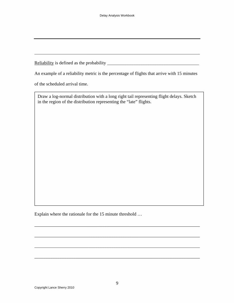
Reliability is defined as the probability ________________________________________

An example of a reliability metric is the percentage of flights that arrive with 15 minutes

of the scheduled arrival time.

Explain where the rationale for the 15 minute threshold …

________________________________________________________________________

________________________________________________________________________

________________________________________________________________________

________________________________________________________________________

Draw a log-normal distribution with a long right tail representing flight delays. Sketch in the region of the distribution representing the “late” flights.



Maximum Queue Length is used by designers to determine the amount of space (e.g.

taxiway lengths for departure queue) that should be provided to handle the maximum

queue. This parameter is measure of the risk of the exceeding the maximum queue length.

Describe the two approaches used to compute Maximum Queue Length;

1) _____________________________________________________________________

________________________________________________________________________

________________________________________________________________________

2) _____________________________________________________________________

________________________________________________________________________

________________________________________________________________________



STOCHASTIC QUEUING BEHAVIOR

Read 23-4 and 23-6

Page 842

Stochastic delays occur when the demand rate is less than the available capacity (i.e. ρ

____ 1). This is due the _____________________________ in the demand inter-arrival

times and/or service times. These arrival clusters appear due to _________________

and/or ________________________.

As ρ approaches 1 over a long period, the stochastic delays can be come significant.

Stochastic queuing systems are analyzed under _____________________ conditions.

Explain this term _____________________________________________________

___________________________________________________________________

____________________________________________________________________

Explain the term steady state _____________________________________________

_____________________________________________________________________

_____________________________________________________________________

Little’s Law is a description of ______________________________________________

Page 843

Little’s Law

Little’s Law computes the following 4 parameters:

1. Total Amount of Time Spent by a User in the Queue represented by ______

2. Total Number of Users in the Queuing System, represented by ___________



3. Waiting Time for a User, represented by Wq

4. Number of Users in the Queue, represented by N

W = sum of amount of time a user spends in the queue and being serviced (Wq).

N = sum of _______________________________________________________

Keep in mind, each of the 4 parameters are random variables. When a queuing system is

in steady-state the expected values (i.e. averages) of the random variables satisfy the

following relationships:

1. E[N] = λ * E[W]

2. E[Nq] = = λ * E[Wq]

3. E[W] = E[Wq] + (1/µ)

Explain each of the relationships above:

1. __________________________________________________________________

________________________________________________________________________

________________________________________________________________________

________________________________________________________________________

2. __________________________________________________________________

________________________________________________________________________

________________________________________________________________________

________________________________________________________________________

3. __________________________________________________________________

________________________________________________________________________

________________________________________________________________________

________________________________________________________________________



Congestion vs Utilization

Page 843+

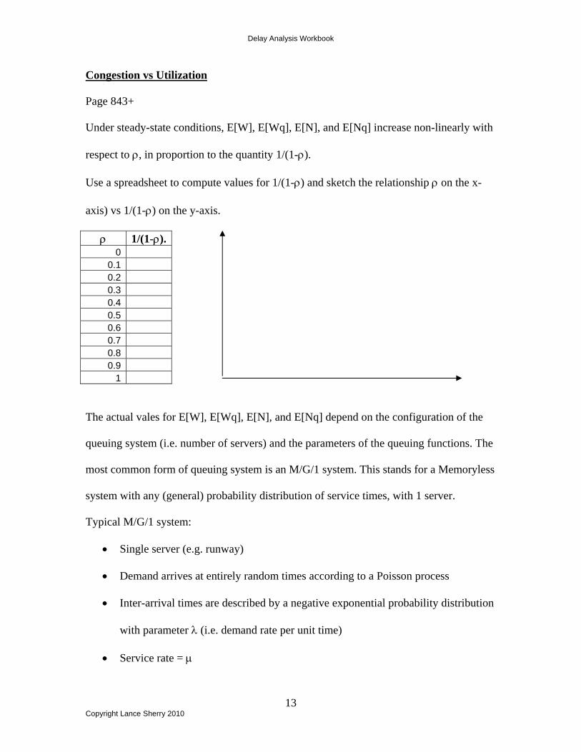
Under steady-state conditions, E[W], E[Wq], E[N], and E[Nq] increase non-linearly with

respect to ρ, in proportion to the quantity 1/(1-ρ).

Use a spreadsheet to compute values for 1/(1-ρ) and sketch the relationship ρ on the x-

axis) vs 1/(1-ρ) on the y-axis.

ρ 1/(1-ρ). 0

0.1 0.2 0.3 0.4 0.5 0.6 0.7 0.8 0.9

1

The actual vales for E[W], E[Wq], E[N], and E[Nq] depend on the configuration of the

queuing system (i.e. number of servers) and the parameters of the queuing functions. The

most common form of queuing system is an M/G/1 system. This stands for a Memoryless

system with any (general) probability distribution of service times, with 1 server.

Typical M/G/1 system:

• Single server (e.g. runway)

• Demand arrives at entirely random times according to a Poisson process

• Inter-arrival times are described by a negative exponential probability distribution

with parameter λ (i.e. demand rate per unit time)

• Service rate = µ



• Service time S, has variance σ2(S)

• System has infinite queuing capacity (e.g. taxiway holds all aircraft submitted to a

departure runway queue).

E[Wq] = __________________________________________

E[Wq] = __________________________________________

Now that you have computed E[Wq] you can compute

E[W] = E[Wq] + (1/µ)

Then you can compute,

E[N] = λ * E[W]

E[Nq] = = λ * E[Wq]

Note 1: the expression for E[Wq] includes the term 1/(1-ρ). This term is a dominant

factor in the equations and determines the overall shape of the function.

Note 2: the σ2(S) term, the variability in Service times determines how fast the E[.]

grow. In general, the higher the variability in inter-arrival times (i.e. bunching or

arrivals represented by λ) or the higher the variability in service times (σ2(S)), the

faster E[.] increases.

Exercise #1: Study the relationship between Service Time variability and Average

Number of Users in the Queue.



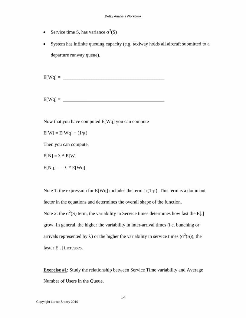
Use a spreadsheet to compute and chart the values for ρ vs E[Nq]. Assume an M/G/1

system. See table below. Explain the difference in E[Nq] between system A and B.

What are the design implications of this result?

System A µ = 60 per hour

(σ2(S) = 0

System B µ = 60 per hour (σ2(S) = 0.81

ρ E[Wq] E[Nq] E[Wq] E[Nq] 0

0.1 0.2 0.3 0.4 0.5 0.6 0.7 0.8 0.9

1

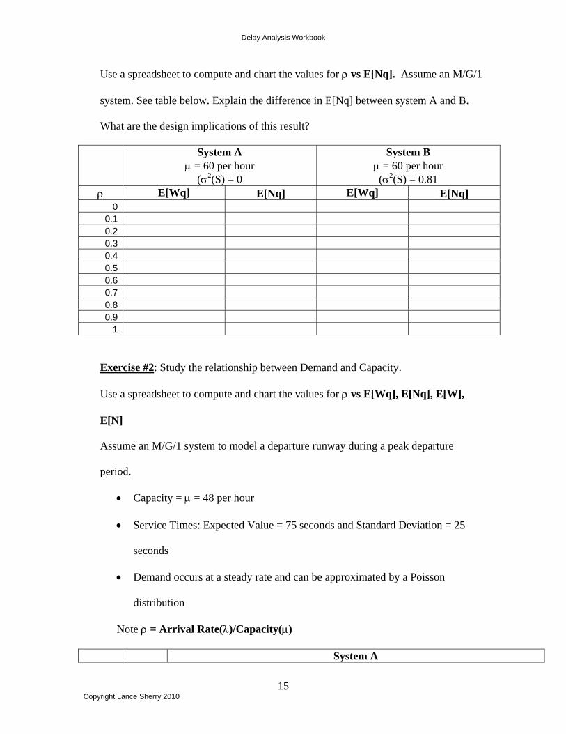
Exercise #2: Study the relationship between Demand and Capacity.

Use a spreadsheet to compute and chart the values for ρ vs E[Wq], E[Nq], E[W],

E[N]

Assume an M/G/1 system to model a departure runway during a peak departure

period.

• Capacity = µ = 48 per hour

• Service Times: Expected Value = 75 seconds and Standard Deviation = 25

seconds

• Demand occurs at a steady rate and can be approximated by a Poisson

distribution

Note ρ = Arrival Rate(λ)/Capacity(µ)

System A



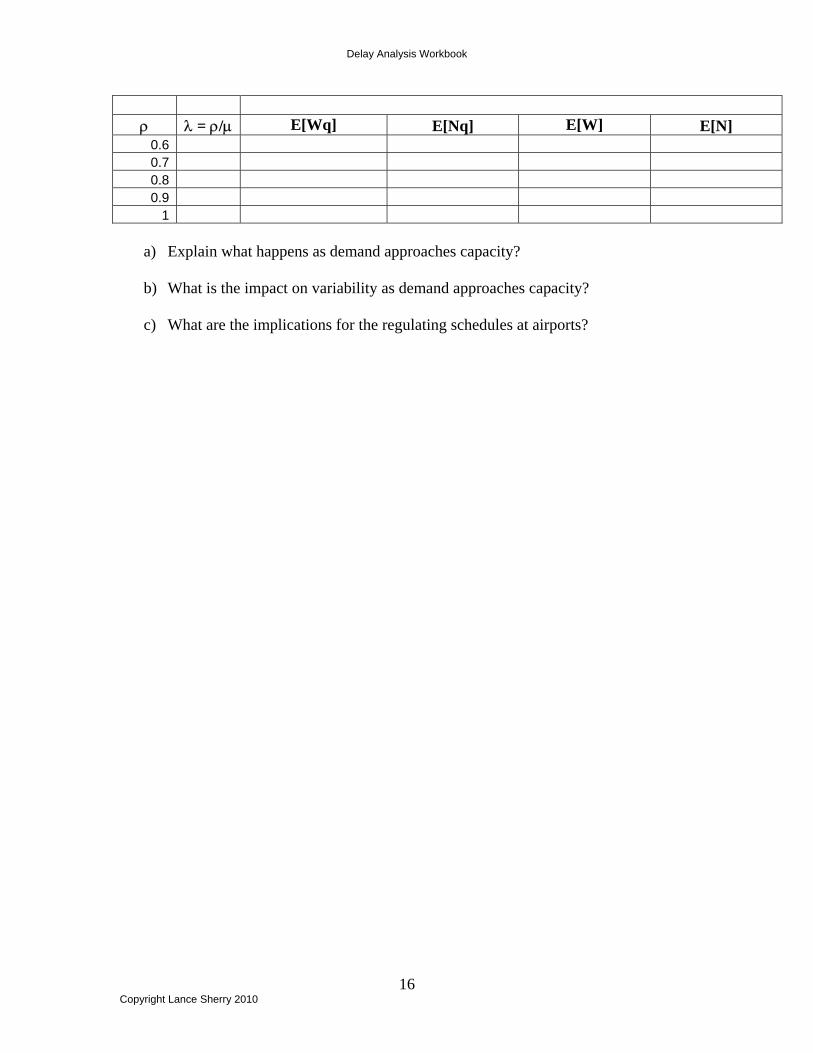
ρ λ = ρ/µ E[Wq] E[Nq] E[W] E[N]

0.6 0.7 0.8 0.9

1

a) Explain what happens as demand approaches capacity?

b) What is the impact on variability as demand approaches capacity?

c) What are the implications for the regulating schedules at airports?



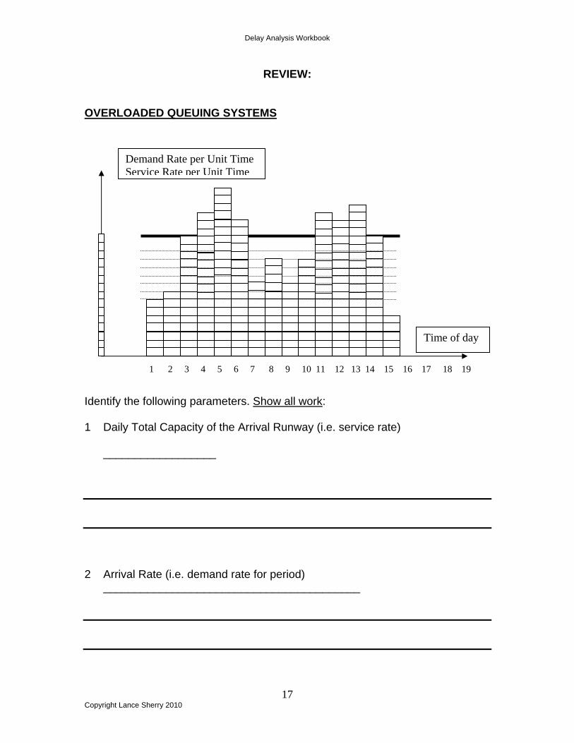
REVIEW: OVERLOADED QUEUING SYSTEMS

Identify the following parameters. Show all work: 1 Daily Total Capacity of the Arrival Runway (i.e. service rate)

__________________

2 Arrival Rate (i.e. demand rate for period)

_________________________________________

Demand Rate per Unit Time Service Rate per Unit Time

1 2 3 4 5 6 7 8 9 10 11 12 13 14 15 16 17 18 19

Time of day



3 Daily Total Demand for the Arrival Runway

________________________________

4 Time periods with Demand in excess of Capacity

___________________________

5 Time periods in which flights will be delayed

_______________________________

6 Daily Total Demand over Capacity Ratio

_________________________________

7 Do you expect to delays to occur? Why

___________________________________



______________________________________________________________________



Learning Objectives:

1. Understand the dynamics of delays that result from over-scheduled

resources

2. Understand the impact of “exemptions” to the dynamics of delays that

result from over-scheduled resources

3. Understand the impact of “cancellations” to the dynamics of delays that


4. Understand the impact of “cancellations with compression” to the

dynamics of delays that result from over-scheduled resources

5. Understand the impact of “slot swapping” to the dynamics of delays that


6. Understand the implications of over-scheduled resources on Proportional

Equity

7. Understand the canonical form of the equations for overscheduled

resources



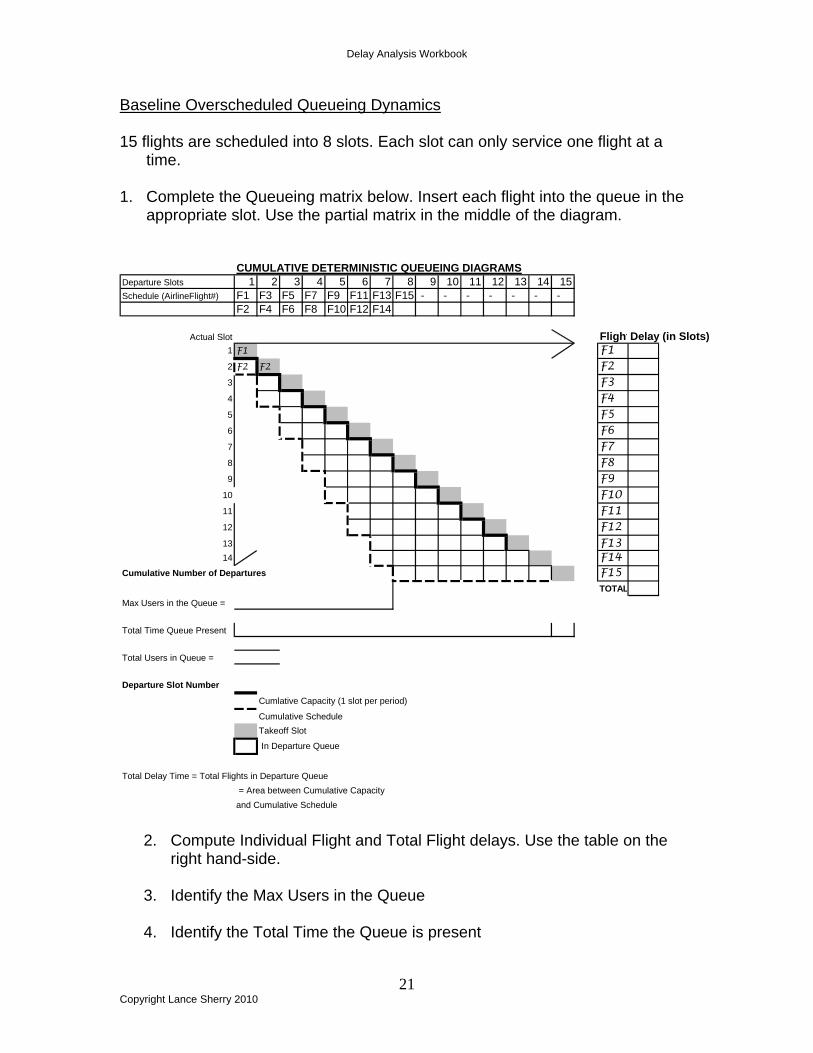
Baseline Overscheduled Queueing Dynamics 15 flights are scheduled into 8 slots. Each slot can only service one flight at a

time. 1. Complete the Queueing matrix below. Insert each flight into the queue in the

appropriate slot. Use the partial matrix in the middle of the diagram.

CUMULATIVE DETERMINISTIC QUEUEING DIAGRAMSDeparture Slots 1 2 3 4 5 6 7 8 9 10 11 12 13 14 15Schedule (AirlineFlight#) F1 F3 F5 F7 F9 F11 F13 F15 - - - - - - -

F2 F4 F6 F8 F10 F12 F14

Actual Slot FlightDelay (in Slots)1 F1 F1 02 F2 F2 F2 13 F3 F3 F3 14 F4 F4 F4 F4 25 F5 F5 F5 F5 26 F6 F6 F6 F6 F6 37 F7 F7 F7 F7 F7 38 F8 F8 F8 F8 F8 F8 49 F9 F9 F9 F9 F9 F9 4

10 F10 F10 F10 F10 F10 F10 F10 511 F11 F11 F11 F11 F11 F11 F11 512 F12 F12 F12 F12 F12 F12 F12 F12 613 F13 F13 F13 F13 F13 F13 F13 F13 614 F14 F14 F14 F14 F14 F14 F14 F14 F14 7

Cumulative Number of Departures F15 F15 F15 F15 F15 F15 F15 F15 F15 7TOTAL 56

Max Users in the Queue =

Total Time Queue Present

Total Users in Queue =

Departure Slot Number

Cumlative Capacity (1 slot per period)

Cumulative ScheduleTakeoff Slot

In Departure Queue

Total Delay Time = Total Flights in Departure Queue = Area between Cumulative Capacityand Cumulative Schedule

2. Compute Individual Flight and Total Flight delays. Use the table on the

right hand-side.

3. Identify the Max Users in the Queue 4. Identify the Total Time the Queue is present



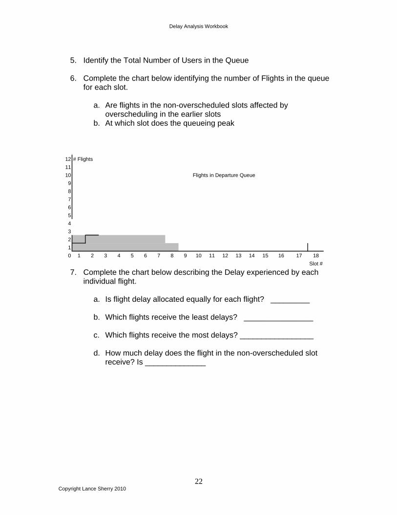
5. Identify the Total Number of Users in the Queue

6. Complete the chart below identifying the number of Flights in the queue

for each slot.

a. Are flights in the non-overscheduled slots affected by overscheduling in the earlier slots

b. At which slot does the queueing peak

12 # Flights1110 Flights in Departure Queue9876543210 1 2 3 4 5 6 7 8 9 10 11 12 13 14 15 16 17 18

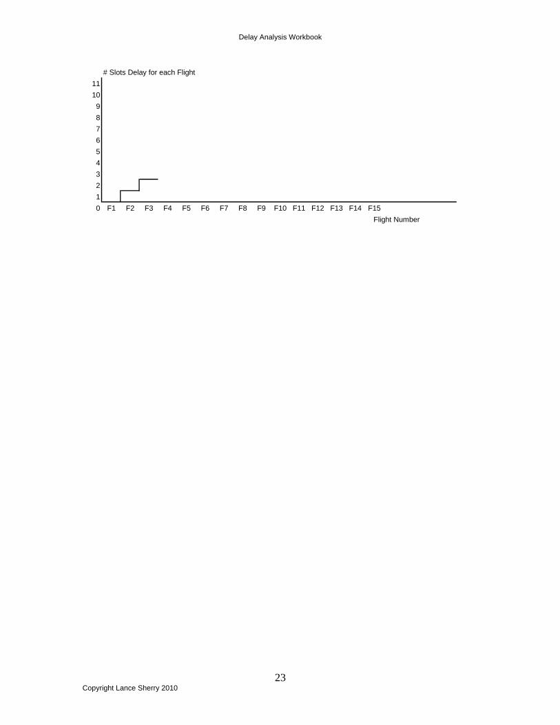
Slot # 7. Complete the chart below describing the Delay experienced by each

individual flight.

a. Is flight delay allocated equally for each flight? _________ b. Which flights receive the least delays? ________________

c. Which flights receive the most delays? _________________

d. How much delay does the flight in the non-overscheduled slot

receive? Is ______________



# Slots Delay for each Flight11109876543210 F1 F2 F3 F4 F5 F6 F7 F8 F9 F10 F11 F12 F13 F14 F15

Flight Number



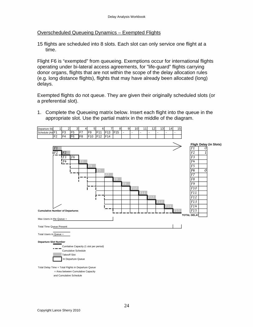
Overscheduled Queueing Dynamics – Exempted Flights 15 flights are scheduled into 8 slots. Each slot can only service one flight at a

time. Flight F6 is “exempted” from queueing. Exemptions occur for international flights operating under bi-lateral access agreements, for ”life-guard” flights carrying donor organs, flights that are not within the scope of the delay allocation rules (e.g. long distance flights), flights that may have already been allocated (long) delays. Exempted flights do not queue. They are given their originally scheduled slots (or a preferential slot). 1. Complete the Queueing matrix below. Insert each flight into the queue in the

appropriate slot. Use the partial matrix in the middle of the diagram. Departure Slo 1 2 3 4 5 6 7 8 9 10 11 12 13 14 15Schedule (Air F1 F3 F5 F7 F9 F11 F13 F15 - - - - - - -

F2 F4 F6 F8 F10 F12 F14

FlightDelay (in Slots)F1 F1 0F2 F2 F2 1

F3 F6 F3 2F4 F3 F3 F4 3

F4 F4 F4 F5 3F5 F5 F5 F5 F6 0

F7 F7 F7 F7 F7 3F8 F8 F8 F8 F8 F8 4

F9 F9 F9 F9 F9 F9 4F10 F10 F10 F10 F10 F10 F10 5

F11 F11 F11 F11 F11 F11 F11 5F12 F12 F12 F12 F12 F12 F12 F12 6

F13 F13 F13 F13 F13 F13 F13 F13 6F14 F14 F14 F14 F14 F14 F14 F14 F14 7

Cumulative Number of Departures F15 F15 F15 F15 F15 F15 F15 F15 F15 7TOTAL DELAY 56




Departure Slot Number

Cumlative Capacity (1 slot per period)

Cumulative ScheduleTakeoff Slot

In Departure Queue




2. Compute Individual Flight and Total Flight delays. Use the table on the right hand-side. How do Total Flight Delays compare with the Baseline queueing? Explain.

3. Identify the Max Users in the Queue. Compare to Baseline queueing?

Explain.

4. Identify the Total Time the Queue is present. Compare to Baseline

queueing? Explain.

5. Identify the Total Number of Users in the Queue. Compare to Baseline

queueing? Explain.



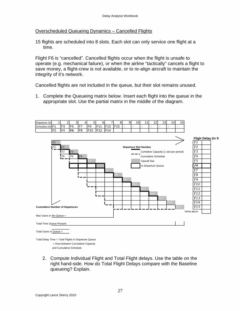
Overscheduled Queueing Dynamics – Cancelled Flights 15 flights are scheduled into 8 slots. Each slot can only service one flight at a

time. Flight F6 is “cancelled”. Cancelled flights occur when the flight is unsafe to operate (e.g. mechanical failure), or when the airline “tactically” cancels a flight to save money, a flight-crew is not available, or to re-align aircraft to maintain the integrity of it’s network. Cancelled flights are not included in the queue, but their slot remains unused. 1. Complete the Queueing matrix below. Insert each flight into the queue in the

appropriate slot. Use the partial matrix in the middle of the diagram. Departure Slo 1 2 3 4 5 6 7 8 9 10 11 12 13 14 15Schedule (Air F1 F3 F5 F7 F9 F11 F13 F15 - - - - - - -

F2 F4 F6 F8 F10 F12 F14

FlightDelay (in SF1 F1 0F2 F2 Departure Slot Number F2 1

F3 F3 Cumlative Capacity (1 slot per period) F3 1F4 F4 F4 Cumulative Schedule F4 2

F5 F5 F5 Takeoff Slot F5 2 In Departure Queue F6 0

F7 F7 F7 F7 F7 3F8 F8 F8 F8 F8 F8 4

F9 F9 F9 F9 F9 F9 4F10 F10 F10 F10 F10 F10 F10 5


F13 F13 F13 F13 F13 F13 F13 F13 6F14 F14 F14 F14 F14 F14 F14 F14 F14 7

Cumulative Number of Departures F15 F15 F15 F15 F15 F15 F15 F15 F15 7TOTAL DELAY 53






right hand-side. How do Total Flight Delays compare with the Baseline queueing? Explain.




Explain.


queueing? Explain.


queueing? Explain.



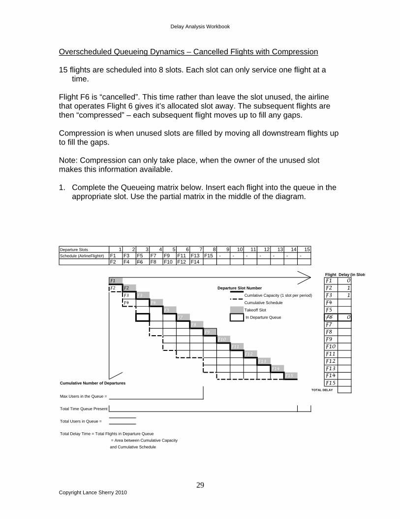
Overscheduled Queueing Dynamics – Cancelled Flights with Compression 15 flights are scheduled into 8 slots. Each slot can only service one flight at a

time. Flight F6 is “cancelled”. This time rather than leave the slot unused, the airline that operates Flight 6 gives it’s allocated slot away. The subsequent flights are then “compressed” – each subsequent flight moves up to fill any gaps. Compression is when unused slots are filled by moving all downstream flights up to fill the gaps. Note: Compression can only take place, when the owner of the unused slot makes this information available. 1. Complete the Queueing matrix below. Insert each flight into the queue in the

appropriate slot. Use the partial matrix in the middle of the diagram. Departure Slots 1 2 3 4 5 6 7 8 9 10 11 12 13 14 15Schedule (AirlineFlight#) F1 F3 F5 F7 F9 F11 F13 F15 - - - - - - -

F2 F4 F6 F8 F10 F12 F14

Flight Delay (in SlotsF1 F1 0F2 F2 Departure Slot Number F2 1


F5 F5 F5 Takeoff Slot F5 2F7 F7 F7 In Departure Queue F6 0F8 F8 F8 F8 F7 2

F9 F9 F9 F9 F8 3F10 F10 F10 F10 F10 F9 3

F11 F11 F11 F11 F11 F10 4F12 F12 F12 F12 F12 F12 F11 4


F15 F15 F15 F15 F15 F15 F15 F14 6Cumulative Number of Departures F15 6

TOTAL DELAY 44Max Users in the Queue =








3. Identify the Max Users in the Queue. Compare to Baseline queueing? Explain.

4. Identify the Total Time the Queue is present. Compare to Baseline queueing? Explain.


queueing? Explain.

6. Under what conditions would the operator of flight F6 gain by giving up their unused slot?Explain.



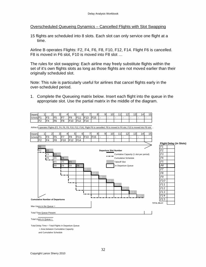
Overscheduled Queueing Dynamics – Cancelled Flights with Slot Swapping 15 flights are scheduled into 8 slots. Each slot can only service one flight at a

time. Airline B operates Flights: F2, F4, F6, F8, F10, F12, F14. Flight F6 is cancelled. F8 is moved in F6 slot, F10 is moved into F8 slot … The rules for slot swapping: Each airline may freely substitute flights within the set of it’s own flights slots as long as those flights are not moved earlier than their originally scheduled slot. Note: This rule is particularly useful for airlines that cancel flights early in the over-scheduled period. 1. Complete the Queueing matrix below. Insert each flight into the queue in the

appropriate slot. Use the partial matrix in the middle of the diagram. Departu 1 2 3 4 5 6 7 8 9 10 11 12 13 14 15Schedu F1 F3 F5 F7 F9 F11 F13 F15 - - - - - - -

F2 F4 F6 F8 F10 F12 F14

Airline B operates Flights (F2, F4, F6, F8, F10, F12, F14). Flight F6 is cancelled. F8 is moved in F6 slot, F10 is moved into F8 slot …

Departu 1 2 3 4 5 6 7 8 9 10 11 12 13 14 15Schedu F1 F3 F5 F7 F9 F11 F13 F15 - - - - - - -

F2 F4 F8 F10 F12 F14Flight Delay (in Slots)

F1 F1 0F2 F2 Departure Slot Number F2 1


F5 F5 F5 Takeoff Slot F5 2F8 F8 F8 F8 In Departure Queue F6 0

F7 F7 F7 F7 F7 3F10 F10 F10 F10 F10 F8 3

F9 F9 F9 F9 F9 F9 4F12 F12 F12 F12 F12 F12 F10 4


F13 F13 F13 F13 F13 F13 F13 F13 6F15 F15 F15 F15 F15 F15 F15 F14 6

Cumulative Number of Departures F15 6TOTAL DELAY 48










Explain.


queueing? Explain.


queueing? Explain.



6. Under what conditions would the operator of flight F6 gain by giving up their unused slot? Explain.



Equity Every society has rules for sharing goods and burdens among it’s members (Young,1994). Some resources are managed through property rights and liabilities that are held and traded by private individuals or held by enterprises according to complex financial regulations. Other property rights are held by a governing entity and allocated according to societal needs. The mechanism for the distribution of property rights expresses the notions of equity in the division of the resources deemed reasonable by societal norms. The appropriateness of the equity is determined in part by principle and in part by precedent. There are three main decisions that must be made in the allocation of commonly held property: (1) the supply decision determines the amount of resources to be distributed (e.g. arrival slots). (2) the distributive decision determines the principles and methods used to allocate the resources (e.g. first-scheduled/first-served), and (3) the reactive decision: determines the owners or users to the allocation scheme (e.g. slot substitutions and slot swapping). The focus of this paper is the implications of the distributive decision. Varieties of Equity Equitable allocation should be a simple process. Each party is allocated an equal distribution measured according to a single yardstick. The reality is that allocated resources are not equal. Claimant parties are in different situations and the agreement of single yardstick is difficult to achieve (Rae 1981). A wide range of philosophers (e.g. Aristotle, Maimonides) have examined the “combinatorics” of allocation of asymmetric resources to claimants using various yardsticks. These philosophers have developed appropriate allocation schemes for specific combinations. One of the emergent themes of these allocation schemes is that the equity formulas are usually based, either explicitly or implicitly, on a standard of comparison that ranks the various claimants on their relative desert (Young, 1994; pg 80). Proportionality and Proportional Equity One of the oldest and most widely used distributive principles is one that ranks claimants rights. This is the “Principle of Proportionality.” Proportionality is implicit in the mechanism of First-Come/First-Serve used in Air Traffic Control (ATC) and is the explicit in the mechanism of First-Scheduled/First-Served used in Traffic Flow Management (ATFM). This principle allocates the resources in proportion to the demand for the resource such that groups (e.g. airlines, passengers with specific demographics, or flights with specific emissive properties) will receive delays in proportion to their number of flights scheduled. Proportional Equity is defined by the following equation:



Proportional Equity for Group (i) = [Total Delay for Group (i) / Total Delay for all Groups] / [Number of Flights for Group (i) / Total Flights for all Groups] where i are groups of users (e.g. airlines) 1 through n.

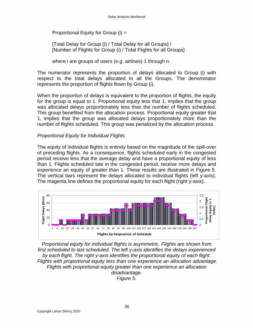
The numerator represents the proportion of delays allocated to Group (i) with respect to the total delays allocated to all the Groups. The denominator represents the proportion of flights flown by Group (i). When the proportion of delays is equivalent to the proportion of flights, the equity for the group is equal to 1. Proportional equity less that 1, implies that the group was allocated delays proportionately less than the number of flights scheduled. This group benefited from the allocation process. Proportional equity greater that 1, implies that the group was allocated delays proportionately more than the number of flights scheduled. This group was penalized by the allocation process. Proportional Equity for Individual Flights The equity of individual flights is entirely based on the magnitude of the spill-over of preceding flights. As a consequence, flights scheduled early in the congested period receive less that the average delay and have a proportional equity of less than 1. Flights scheduled late in the congested period, receive more delays and experience an equity of greater than 1. These results are illustrated in Figure 5. The vertical bars represent the delays allocated to individual flights (left y-axis). The magenta line defines the proportional equity for each flight (right y-axis).

Proportional equity for individual flights is asymmetric. Flights are shown from

first scheduled to last scheduled. The left y-axis identifies the delays experienced by each flight. The right y-axis identifies the proportional equity of each flight.

Flights with proportional equity less than one experience an allocation advantage. Flights with proportional equity greater than one experience an allocation

disadvantage. Figure 5.

0

20

40

60

80

1 8 15 22 29 36 43 50 57 64 71 78 85 92 99 106 113 120 127 134 141 148 155 162 169 176 183 190 197

Flights by Seqeuence of Schedule

Flig

ht D

elay

s (M

ins)

0

0.5

1

1.5

2

2.5

Prop

ortio

nal F

light

D

elay

Equ

ity (>

1

Unf

air)



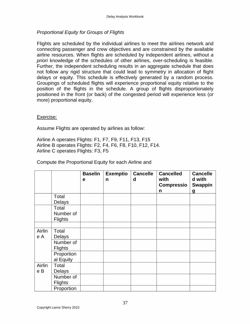
Proportional Equity for Groups of Flights Flights are scheduled by the individual airlines to meet the airlines network and connecting passenger and crew objectives and are constrained by the available airline resources. When flights are scheduled by independent airlines, without a priori knowledge of the schedules of other airlines, over-scheduling is feasible. Further, the independent scheduling results in an aggregate schedule that does not follow any rigid structure that could lead to symmetry in allocation of flight delays or equity. This schedule is effectively generated by a random process. Groupings of scheduled flights will experience proportional equity relative to the position of the flights in the schedule. A group of flights disproportionately positioned in the front (or back) of the congested period will experience less (or more) proportional equity. Exercise: Assume Flights are operated by airlines as follow: Airline A operates Flights: F1, F7, F9, F11, F13, F15 Airline B operates Flights: F2, F4, F6, F8, F10, F12, F14. Airline C operates Flights: F3, F5 Compute the Proportional Equity for each Airline and Baselin

e Exemption

Cancelled

Cancelled with Compression

Cancelled with Swapping

Total Delays

Total Number of Flights

Total Delays

Number of Flights

Airline A

Proportional Equity

Total Delays

Number of Flights

Airline B

Proportion



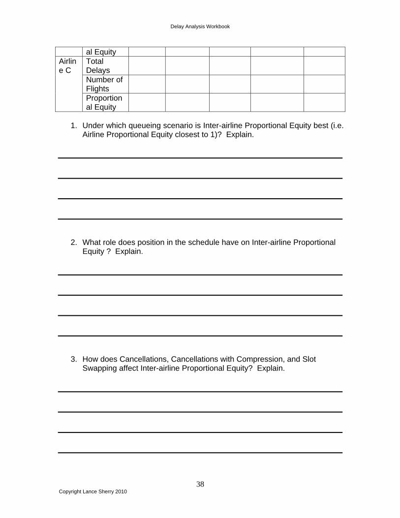
al Equity Total Delays

Number of Flights

Airline C

Proportional Equity

1. Under which queueing scenario is Inter-airline Proportional Equity best (i.e.

Airline Proportional Equity closest to 1)? Explain.

2. What role does position in the schedule have on Inter-airline Proportional Equity ? Explain.

3. How does Cancellations, Cancellations with Compression, and Slot Swapping affect Inter-airline Proportional Equity? Explain.



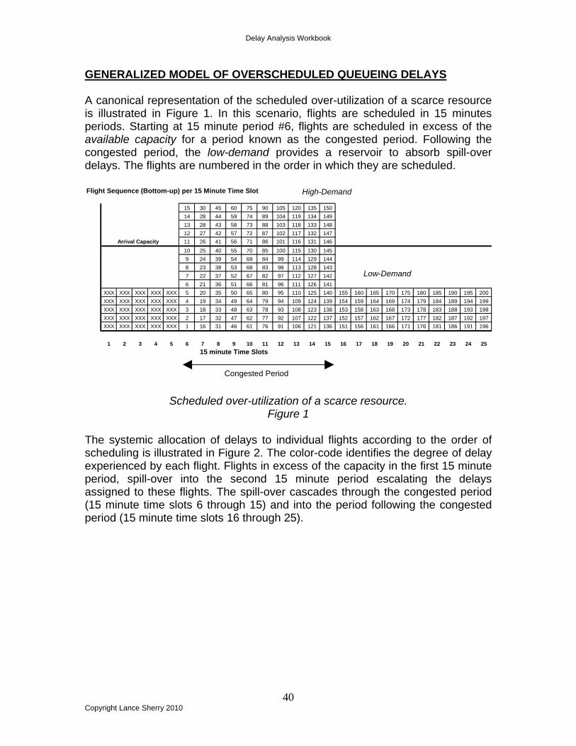
GENERALIZED MODEL OF OVERSCHEDULED QUEUEING DELAYS A canonical representation of the scheduled over-utilization of a scarce resource is illustrated in Figure 1. In this scenario, flights are scheduled in 15 minutes periods. Starting at 15 minute period #6, flights are scheduled in excess of the available capacity for a period known as the congested period. Following the congested period, the low-demand provides a reservoir to absorb spill-over delays. The flights are numbered in the order in which they are scheduled.

Scheduled over-utilization of a scarce resource. Figure 1

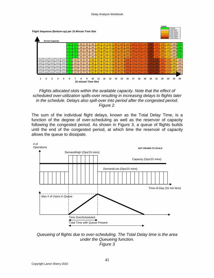
The systemic allocation of delays to individual flights according to the order of scheduling is illustrated in Figure 2. The color-code identifies the degree of delay experienced by each flight. Flights in excess of the capacity in the first 15 minute period, spill-over into the second 15 minute period escalating the delays assigned to these flights. The spill-over cascades through the congested period (15 minute time slots 6 through 15) and into the period following the congested period (15 minute time slots 16 through 25).

Flight Sequence (Bottom-up) per 15 Minute Time Slot

15 30 45 60 75 90 105 120 135 15014 28 44 59 74 89 104 119 134 14913 28 43 58 73 88 103 118 133 14812 27 42 57 72 87 102 117 132 147

Arrival Capacity 11 26 41 56 71 86 101 116 131 14610 25 40 55 70 85 100 115 130 1459 24 39 54 69 84 99 114 129 1448 23 38 53 68 83 98 113 128 1437 22 37 52 67 82 97 112 127 1426 21 36 51 66 81 96 111 126 141

XXX XXX XXX XXX XXX 5 20 35 50 65 80 95 110 125 140 155 160 165 170 175 180 185 190 195 200XXX XXX XXX XXX XXX 4 19 34 49 64 79 94 109 124 139 154 159 164 169 174 179 184 189 194 199XXX XXX XXX XXX XXX 3 18 33 48 63 78 93 108 123 138 153 158 163 168 173 178 183 188 193 198XXX XXX XXX XXX XXX 2 17 32 47 62 77 92 107 122 137 152 157 162 167 172 177 182 187 192 197XXX XXX XXX XXX XXX 1 16 31 46 61 76 91 106 121 136 151 156 161 166 171 176 181 186 191 196

1 2 3 4 5 6 7 8 9 10 11 12 13 14 15 16 17 18 19 20 21 22 23 24 2515 minute Time Slots

High-Demand

Low-Demand

Congested Period



Flights allocated slots within the available capacity. Note that the effect of scheduled over-utilization spills-over resulting in increasing delays to flights later

in the schedule. Delays also spill-over into period after the congested period. Figure 2.

The sum of the individual flight delays, known as the Total Delay Time, is a function of the degree of over-scheduling as well as the reservoir of capacity following the congested period. As shown in Figure 3, a queue of flights builds until the end of the congested period, at which time the reservoir of capacity allows the queue to dissipate.

Queueing of flights due to over-scheduling. The Total Delay time is the area under the Queueing function.

Figure 3

Flight Sequence (Bottom-up) per 15 Minute Time Slot

Arrival Capacity10 20 30 40 50 60 70 80 90 100 110 120 130 140 150 160 170 180 190 2009 19 29 39 49 59 69 79 89 99 109 119 129 139 149 159 169 179 189 1998 18 28 38 48 58 68 78 88 98 108 118 128 138 148 158 168 178 188 1987 17 27 37 47 57 67 77 87 97 107 117 127 137 147 157 167 177 187 1976 16 26 36 46 56 66 76 86 96 106 116 126 136 146 156 166 176 186 196

XXX XXX XXX XXX XXX 5 15 25 35 45 55 65 75 85 95 105 115 125 135 145 155 165 175 185 195XXX XXX XXX XXX XXX 4 14 24 34 44 54 64 74 84 94 104 114 124 134 144 154 164 174 184 194XXX XXX XXX XXX XXX 3 13 23 33 43 53 63 73 83 93 103 113 123 133 143 153 163 173 183 193XXX XXX XXX XXX XXX 2 12 22 32 42 52 62 72 82 92 102 112 122 132 142 152 162 172 182 192XXX XXX XXX XXX XXX 1 11 21 31 41 51 61 71 81 91 101 111 121 131 141 151 161 171 181 191

1 2 3 4 5 6 7 8 9 10 11 12 13 14 15 16 17 18 19 20 21 22 23 24 2515 minute Time Slot

LegendNo Delay15 Min Dely30 Min Delay45 Min Delay60 Min Delay75 Min Delay

Time-of-Day (15 min bins)

# of Operations

Capacity (Ops/15 mins)

DemandLow (Ops/15 mins)

DemandHigh (Ops/15 mins)

Time OverScheduled

Total Time with Queue Present

Max # of Users in Queue

NOT DRAWN TO SCALE



The Total Delay Time resulting from the scheduled utilization is defined by the equation:

Total Delay Time = ½ * (Duration of Congested Period)2* (HighDemand – Capacity) * [1 + HighDemand – Capacity ] Capacity – LowDemand

This equation is derived by calculating the area under the queue curve in Figure 3. The equation highlights the following properties:

(1) Conservation of Total Delays. The Total Delay is independent of the order of the flights. The Total Delay is dependent on the relationship amongst the four terms: Capacity, High_Demand, Low_Demand and Conegsted_Period. Saying this another way, the only way to reduce the Total Delay is to remove flights.

(2) Duration of Congested Period is Critical The factor in the equation that has the biggest effect is the duration of the congested period (TCongestedPeriod). This term is squared. For every additional unit of time in the congested period, the Total Delays increase geometrically.

(3) Reservoirs are Critical: The Total Delays is not only dependent on the degree of over-scheduling, but also on the degree of under-scheduling after the congested period. The degree of under-scheduling provides a reservoir to absorb the spill-over from the congested period. A low degree of under-scheduling can result in extending the queue significantly.

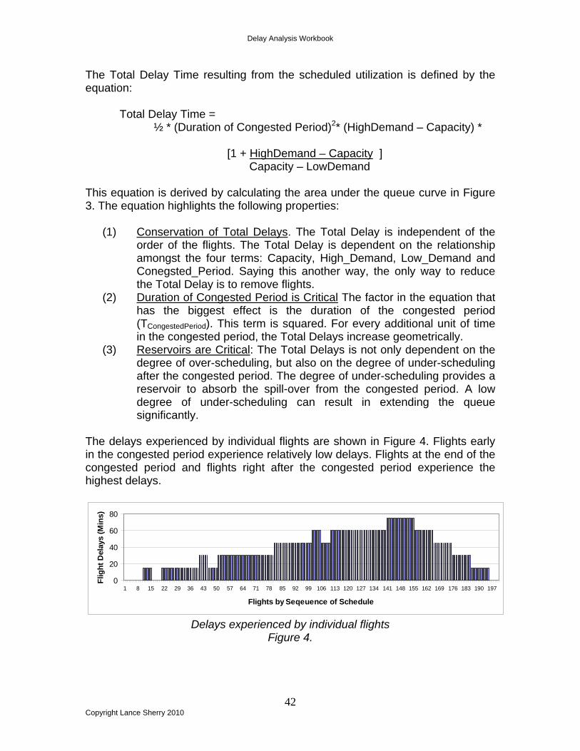
The delays experienced by individual flights are shown in Figure 4. Flights early in the congested period experience relatively low delays. Flights at the end of the congested period and flights right after the congested period experience the highest delays.

Delays experienced by individual flights

Figure 4.

0

20

40

60

80

1 8 15 22 29 36 43 50 57 64 71 78 85 92 99 106 113 120 127 134 141 148 155 162 169 176 183 190 197

Flights by Seqeuence of Schedule

Flig

ht D

elay

s (M

ins)



(4) Asymmettry of Individual Flight Delays: The delays assigned to individual flights are a function of the location of the flight in the schedule. Flights scheduled early in the congested period, are allocated less delays than those flights later in the congested period.

Max Users in Queue = (DemandHigh – Capacity) * TOverScheduled Determined by:

• Degree of Over-scheduling • Duration of Over-scheduling

Total Time Queue Present = TOverScheduled + (DemandHigh – Capacity) * TOverScheduled (Capacity – DemandLow) Spill-over effect depends on degree of over scheduling and available capacity after the over-scheduled slots Total Users in Queue = //Users in the Overscheduled region minus the 1st batch that do not queue [ TOverScheduled * (DemandHigh) ] – [1 * Capacity] + //Users in the duration of the queue [ (DemandHigh – Capacity) * TOverScheduled ] * DemandLow (Capacity – DemandLow) Exercise:



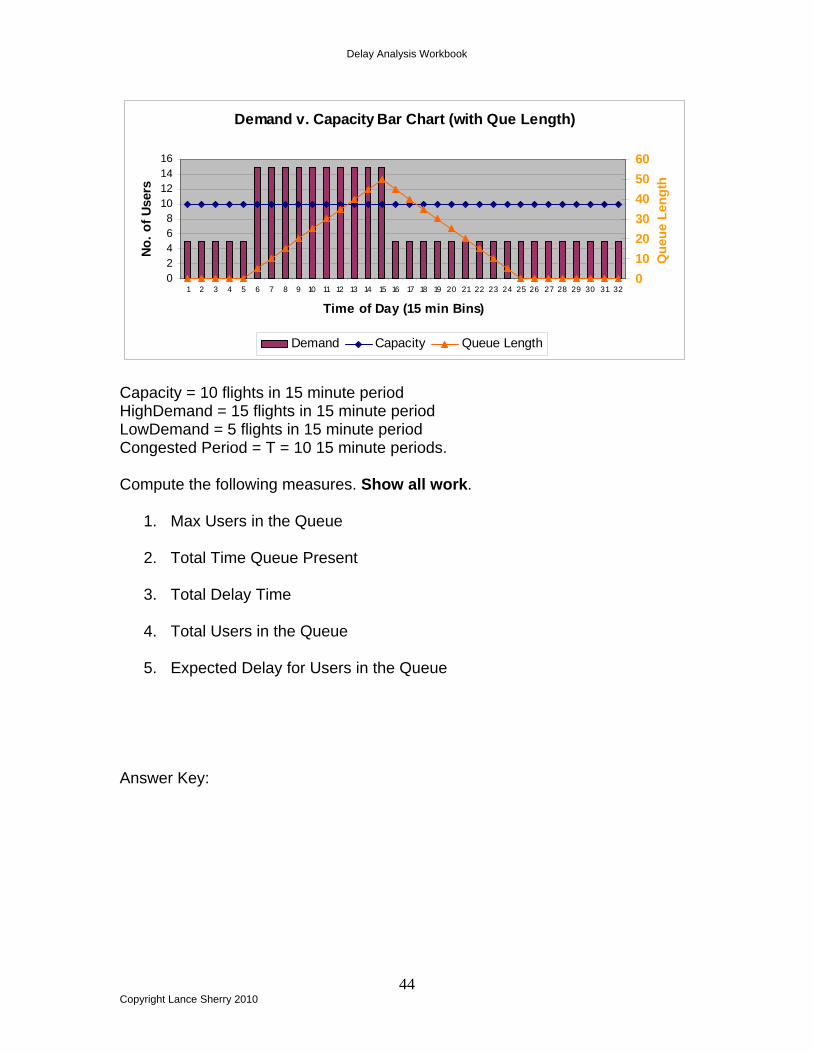
Demand v. Capacity Bar Chart (with Que Length)

02468

10121416

1 2 3 4 5 6 7 8 9 10 11 12 13 14 15 16 17 18 19 20 21 22 23 24 25 26 27 28 29 30 31 32

Time of Day (15 min Bins)

No. o

f Use

rs

0102030405060

Que

ue L

engt

h

Demand Capacity Queue Length

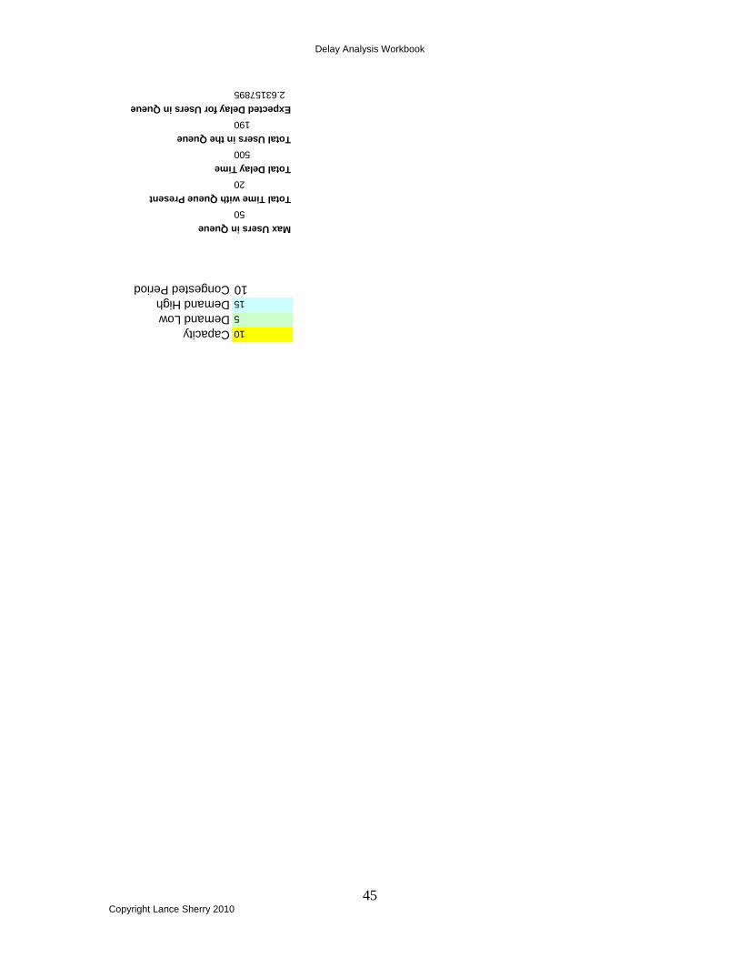
Capacity = 10 flights in 15 minute period HighDemand = 15 flights in 15 minute period LowDemand = 5 flights in 15 minute period Congested Period = T = 10 15 minute periods. Compute the following measures. Show all work.

1. Max Users in the Queue

2. Total Time Queue Present

3. Total Delay Time

4. Total Users in the Queue

5. Expected Delay for Users in the Queue

Answer Key:



10Capacity5Demand Low

15Demand High10Congested Period

Max Users in Queue50

Total Time with Queue Present20

Total Delay Time500

Total Users in the Queue190

Expected Delay for Users in Queue2.63157895

air transportation systems engineering delay analysis …delay analysis workbook . delay analysis...

Documents