airborne and ground-based measurements of the trace gases

Atmos. Chem. Phys., 11, 12197–12216, 2011www.atmos-chem-phys.net/11/12197/2011/doi:10.5194/acp-11-12197-2011© Author(s) 2011. CC Attribution 3.0 License.

AtmosphericChemistry

and Physics

Airborne and ground-based measurements of the trace gases andparticles emitted by prescribed fires in the United States

I. R. Burling 1, R. J. Yokelson1, S. K. Akagi1, S. P. Urbanski2, C. E. Wold2, D. W. T. Griffith 3, T. J. Johnson4,J. Reardon2, and D. R. Weise5

1University of Montana, Department of Chemistry, Missoula, MT 59812, USA2USDA Forest Service, Rocky Mountain Research Station, Fire Sciences Laboratory, Missoula, MT 59808, USA3University of Wollongong, Department of Chemistry, Wollongong, New South Wales, Australia4Pacific Northwest National Laboratories, Richland WA 99354, USA5USDA Forest Service, Pacific Southwest Research Station, Riverside, CA, USA

Received: 8 June 2011 – Published in Atmos. Chem. Phys. Discuss.: 30 June 2011Revised: 17 November 2011 – Accepted: 28 November 2011 – Published: 7 December 2011

Abstract. We have measured emission factors for 19 tracegas species and particulate matter (PM2.5) from 14 pre-scribed fires in chaparral and oak savanna in the southwesternUS, as well as conifer forest understory in the southeasternUS and Sierra Nevada mountains of California. These arelikely the most extensive emission factor field measurementsfor temperate biomass burning to date and the only publishedemission factors for temperate oak savanna fuels. This studyhelps to close the gap in emissions data available for tem-perate zone fires relative to tropical biomass burning. Wepresent the first field measurements of the biomass burningemissions of glycolaldehyde, a possible precursor for aque-ous phase secondary organic aerosol formation. We alsomeasured the emissions of phenol, another aqueous phasesecondary organic aerosol precursor. Our data confirm pre-vious observations that urban deposition can impact the NOxemission factors and thus subsequent plume chemistry. Fortwo fires, we measured both the emissions in the convectivesmoke plume from our airborne platform and the unloftedresidual smoldering combustion emissions with our ground-based platform. The smoke from residual smoldering com-bustion was characterized by emission factors for hydrocar-bon and oxygenated organic species that were up to ten timeshigher than in the lofted plume, including high 1,3-butadieneand isoprene concentrations which were not observed in thelofted plume. This should be considered in modeling the air

Correspondence to:R. J. Yokelson([email protected])

quality impacts for smoke that disperses at ground level. Wealso show that the often ignored unlofted emissions can sig-nificantly impact estimates of total emissions. Preliminaryevidence suggests large emissions of monoterpenes in theresidual smoldering smoke. These data should lead to animproved capacity to model the impacts of biomass burningin similar temperate ecosystems.

1 Introduction

Biomass burning is the largest source of primary, fine car-bonaceous particles and a significant source of trace gases inthe global atmosphere (Bond et al., 2004; Crutzen and An-dreae, 1990) and impacts both the chemical composition aswell as the radiative balance of the atmosphere. The ma-jority of biomass burning occurs unregulated in the tropics(Crutzen and Andreae, 1990). In the United States, formalland management programs use prescribed burning to re-duce wildfire hazards, improve wildlife habitats, and increaseaccess (Biswell, 1989; Wade and Lunsford, 1989). Manyfire-adapted ecosystems depend on the regular occurrence offire for survival (Keeley et al., 2009). In these ecosystems,land managers may implement relatively frequent prescribedburning (every 1–4 yr) of small amounts of biomass underconditions with favorable atmospheric dispersion. The tem-perate regions of the southeastern and southwestern US ex-perience both wildfires and prescribed burning; however, therelative proportion of prescribed burns differs between thetwo regions. Even though the annual average area burned

Published by Copernicus Publications on behalf of the European Geosciences Union.

http://creativecommons.org/licenses/by/3.0/

12198 I. R. Burling et al.: Airborne and ground-based measurements of the trace gases and particles

by wildfire in the southeastern US was 479 000 ha for 2001to 2010, another approximately 650 000 ha were burned byprescribed fires. (NIFC, 2011). Wildfire activity was similarin the southwestern US (New Mexico, Arizona, and south-ern California) where on average 364,000 ha burned annu-ally over 2001 to 2010 (NIFC, 2011). However, prescribedfire has been employed much less in the southwest. TheNational Interagency Fire Center reported a 10-yr average(2001–2010) of 77,000 ha (NIFC, 2011) in the southwest,only about 1/10 of the annual prescribed burning in the south-eastern US.

In the US, burned area data are needed to estimate biomassburning emissions for air quality forecasting and to guide thedevelopment of land and air shed management policy. To thisend, fire detection (Giglio et al., 2003) and burn scar (Giglioet al., 2009; Roy et al., 2008; Urbanski et al., 2009a) ob-servations from the MODIS (Moderate Resolution ImagingSpectroradiometer) satellite have seen increasing use to mapburned area. While under optimum conditions MODIS candetect fires as small as 100 m2 (Giglio et al., 2003), in prac-tice, due to various factors (e.g. fire behavior, cloud cover)the detection rate may be less than 20 % for fires<100 ha insize (Urbanski et al., 2009a). The low MODIS detection ratefor small fires is not critical in the western US where largewildfires dominate annual burned area; however, it poses asignificant impediment to the development of fire emissioninventories in the southeast where small, prescribed fires (av-erage size = 60 ha) comprise∼60 % of annual burned area for2001–2010 (NIFC, 2011).

The contribution of these US temperate burning emis-sions is relatively small on the global scale (van der Werf etal., 2010). However, such burns have the potential to im-pact local visibility and local and regional air quality andemissions data from these regions are therefore necessaryfor land managers to devise appropriate prescribed burningstrategies. Comprehensive field measurements of emissionsfrom biomass burning in these regions are relatively scarce.For field measurements of biomass burning emissions an air-borne measurement platform is usually required for samplingflaming combustion emissions due to the lofting of smokefrom convection created by high flame temperatures. In anairborne study, Yokelson et al. (1999) measured ten of themost common trace gas emissions from a wildfire and twoprescribed fires in North Carolina. In other airborne fieldstudies, Cofer et al. (1988), Hegg et al. (1988) and Radkeet al. (1991) measured the emissions of a limited numberof chemical species from burning of chaparral that was im-pacted by deposition of nitrogenous compounds from adja-cent urban areas. Hardy et al. (1996) measured smoke emis-sions from chaparral fires in southern California using in-strumentation suspended from a cable directly over the fires.They reported emission factors (EF) for particulate matter(PM), CO, CO2, CH4, and total non-methane hydrocarbons(NMHC) by combustion process (i.e. flaming, smoldering).

Prolonged smoldering after local convection from theflame front has ceased is often termed “residual smolder-ing combustion” (RSC, Bertschi et al., 2003) and is respon-sible for many of the negative air quality impacts of pre-scribed burning on a local scale (e.g. smoke exposure com-plaints, visibility-limited highway accidents (Achtemeier,2006)). Ground-based systems are usually required for mea-surements of RSC smoke emissions. The emissions fromRSC burning are quite different from those of flaming com-bustion due to the lower combustion efficiency. The strate-gies adopted by land managers for prescribed burning typ-ically minimize the amount of RSC and its impacts on lo-cal populations. In contrast, wildfires normally burn when“fire danger” is at high levels and forest floor moisture is ata minimum (Deeming et al., 1978), often resulting in sig-nificant amounts of RSC. There are usually few or no op-tions for reducing smoke impacts on populated areas fromwildfires. Although not a factor in this study, in some wild-fires, organic soils (peat) may also burn contributing to RSC.Residual smoldering combustion can continue for weeks af-ter initial ignition and can account for a large portion ofthe total biomass consumed in a fire (Bertschi et al., 2003;Rein et al. 2009). Naeher et al. (2006) measured PM2.5and CO from prescribed fires from sites in South Carolinawith large amounts of down, dead fuel to investigate the ef-fects of preburn mechanical mastication. We are unaware ofany other peer-reviewed field measurements of the emissionsfrom RSC in the temperate regions of the US.

Laboratory measurements of the emissions from biomassburning have some advantages over field studies, includingthe application of more extensive instrumentation, highersmoke concentrations leading to potentially more measur-able species, and the ability to sample all the smoke for anentire fire. Also, fuel characteristics and elemental compo-sition are easier to determine in the laboratory. Due to theseadvantages, laboratory measurements are complementary tofield measurements but emissions data from field measure-ments are usually considered more representative of real fires(Christian et al., 2003) since they reflect actual environmen-tal conditions, real fuels, and similar scale fire behavior. Infact, this work is part of a larger study of the emissions ofbiomass burning of fuel types from biomes of the southeast-ern and southwestern US that has included already publishedlaboratory studies (Burling et al., 2010; Hosseini et al., 2010;Roberts et al., 2010; Veres et al., 2010; Warneke et al., 2011).Here we present smoke emissions data from field measure-ments conducted during prescribed fires burning similar fuelsto those collected for the laboratory phase. We also includesmoke measurements of the lofted emissions from aircraftmeasurements and the RSC emissions using ground-basedinstruments that were conducted on the same fire. Such com-prehensive, simultaneous measurements are rare and espe-cially informative. A more detailed comparison between thelaboratory and field measurements, including all instrumen-tation, will be discussed in a future synthesis paper.

Atmos. Chem. Phys., 11, 12197–12216, 2011 www.atmos-chem-phys.net/11/12197/2011/

I. R. Burling et al.: Airborne and ground-based measurements of the trace gases and particles 12199

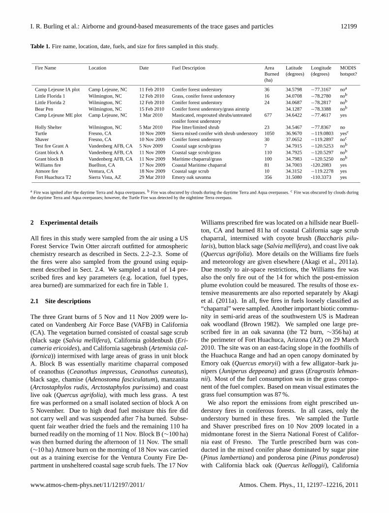
Table 1. Fire name, location, date, fuels, and size for fires sampled in this study.

Fire Name Location Date Fuel Description Area Latitude Longitude MODISBurned (degrees) (degrees) hotspot?(ha)

Camp Lejeune IA plot Camp Lejeune, NC 11 Feb 2010 Conifer forest understory 36 34.5798−77.3167 noa

Little Florida 1 Wilmington, NC 12 Feb 2010 Grass, conifer forest understory 16 34.0708−78.2780 nob

Little Florida 2 Wilmington, NC 12 Feb 2010 Conifer forest understory 24 34.0687−78.2817 nob

Bear Pen Wilmington, NC 15 Feb 2010 Conifer forest understory/grass airstrip 34.1287−78.3388 nob

Camp Lejeune ME plot Camp Lejeune, NC 1 Mar 2010 Masticated, resprouted shrubs/untreated 677 34.6422−77.4617 yesconifer forest understory

Holly Shelter Wilmington, NC 5 Mar 2010 Pine litter/limited shrub 23 34.5467−77.8367 noTurtle Fresno, CA 10 Nov 2009 Sierra mixed conifer with shrub understory 1050 36.9670−119.0803 yesc

Shaver Fresno, CA 10 Nov 2009 Conifer forest understory 30 37.0652−119.2897 noc

Test fire Grant A Vandenberg AFB, CA 5 Nov 2009 Coastal sage scrub/grass 7 34.7915−120.5253 nob

Grant block A Vandenberg AFB, CA 11 Nov 2009 Coastal sage scrub/grass 110 34.7925−120.5297 nob

Grant block B Vandenberg AFB, CA 11 Nov 2009 Maritime chaparral/grass 100 34.7983−120.5250 nob

Williams fire Buellton, CA 17 Nov 2009 Coastal Maritime chaparral 81 34.7003 -120.2083 yesAtmore fire Ventura, CA 18 Nov 2009 Coastal sage scrub 10 34.3152−119.2278 yesFort Huachuca T2 Sierra Vista, AZ 29 Mar 2010 Emory oak savanna 356 31.5080 -110.3373 yes

a Fire was ignited after the daytime Terra and Aqua overpasses.b Fire was obscured by clouds during the daytime Terra and Aqua overpasses.c Fire was obscured by clouds duringthe daytime Terra and Aqua overpasses; however, the Turtle Fire was detected by the nighttime Terra overpass.

2 Experimental details

All fires in this study were sampled from the air using a USForest Service Twin Otter aircraft outfitted for atmosphericchemistry research as described in Sects. 2.2–2.3. Some ofthe fires were also sampled from the ground using equip-ment described in Sect. 2.4. We sampled a total of 14 pre-scribed fires and key parameters (e.g. location, fuel types,area burned) are summarized for each fire in Table 1.

2.1 Site descriptions

The three Grant burns of 5 Nov and 11 Nov 2009 were lo-cated on Vandenberg Air Force Base (VAFB) in California(CA). The vegetation burned consisted of coastal sage scrub(black sage (Salvia mellifera), California goldenbush (Eri-cameria ericoides), and California sagebrush (Artemisia cal-ifornica)) intermixed with large areas of grass in unit blockA. Block B was essentially maritime chaparral composedof ceanothus (Ceanothus impressus, Ceanothus cuneatus),black sage, chamise (Adenostoma fasciculatum), manzanita(Arctostaphylos rudis, Arctostaphylos purissima) and coastlive oak (Quercus agrifolia), with much less grass. A testfire was performed on a small isolated section of block A on5 November. Due to high dead fuel moisture this fire didnot carry well and was suspended after 7 ha burned. Subse-quent fair weather dried the fuels and the remaining 110 haburned readily on the morning of 11 Nov. Block B (∼100 ha)was then burned during the afternoon of 11 Nov. The small(∼10 ha) Atmore burn on the morning of 18 Nov was carriedout as a training exercise for the Ventura County Fire De-partment in unsheltered coastal sage scrub fuels. The 17 Nov

Williams prescribed fire was located on a hillside near Buell-ton, CA and burned 81 ha of coastal California sage scrubchaparral, intermixed with coyote brush (Baccharis pilu-laris), button black sage (Salvia mellifera), and coast live oak(Quercus agrifolia). More details on the Williams fire fuelsand meteorology are given elsewhere (Akagi et al., 2011a).Due mostly to air-space restrictions, the Williams fire wasalso the only fire out of the 14 for which the post-emissionplume evolution could be measured. The results of those ex-tensive measurements are also reported separately by Akagiet al. (2011a). In all, five fires in fuels loosely classified as“chaparral” were sampled. Another important biotic commu-nity in semi-arid areas of the southwestern US is Madreanoak woodland (Brown 1982). We sampled one large pre-scribed fire in an oak savanna (the T2 burn,∼356 ha) atthe perimeter of Fort Huachuca, Arizona (AZ) on 29 March2010. The site was on an east-facing slope in the foothills ofthe Huachuca Range and had an open canopy dominated byEmory oak (Quercus emoryii) with a few alligator–bark ju-nipers (Juniperus deppeana) and grass (Eragrostis lehman-nii). Most of the fuel consumption was in the grass compo-nent of the fuel complex. Based on mean visual estimates thegrass fuel consumption was 87 %.

We also report the emissions from eight prescribed un-derstory fires in coniferous forests. In all cases, only theunderstory burned in these fires. We sampled the Turtleand Shaver prescribed fires on 10 Nov 2009 located in amidmontane forest in the Sierra National Forest of Califor-nia east of Fresno. The Turtle prescribed burn was con-ducted in the mixed conifer phase dominated by sugar pine(Pinus lambertiana) and ponderosa pine (Pinus ponderosa)with California black oak (Quercus kelloggii), California

www.atmos-chem-phys.net/11/12197/2011/ Atmos. Chem. Phys., 11, 12197–12216, 2011


incense cedar (Calocedrus decurrens), and white fir (Abiesconcolor) and a shrub understory of deerbrush (Ceanothusintegerrimus), buckbrush (Ceanothus cuneatus), and prob-ably greenleaf manzanita (Arctostaphylos patula). This firewas ignited using the DAID (Delayed Aerial Ignition Device)system which drops plastic balls containing potassium per-manganate injected with ethylene glycol from a helicopter.The Shaver prescribed burn overstory was dominated byponderosa pine and California incense cedar with scatteredsugar pine and black oak. The understory was dominatedby dense thickets of whiteleaf manzanita (Arctostaphylos vis-cid), bearclover (Chamaebatia foliolosa), with white fir andCalifornia incense cedar regeneration. Due to mountain pinebeetle activity and previous lack of fire, accumulated deadand downed woody fuels exceeded 28 kg m−2. We also sam-pled the smoke from six prescribed fires in pine-dominatedforests in the coastal lowlands of North Carolina (NC) dur-ing February and March of 2010. The 11 February fire atCamp Lejeune (IA plot) had a moderate density coniferousoverstory of loblolly pine (Pinus taeda) and burned under-story fuels, which consisted mainly of fetterbush shrubs (Ly-onia lucida), with some herbaceous fuels. This unit had beenburned∼2–3 yr prior and had light fuel loadings. In addition,due to high fuel moisture, helicopter ignition using the DAIDsystem was required. The second Camp Lejeune (hereafterreferred to as “CL”) fire was on 1 March 2010 (ME plot)and burned through a sequence of several fuel types begin-ning with (1) an area of recently masticated fuels, resproutedfetterbush shrubs and understory hardwoods including redmaple (Acer rubrum) and sweetgum (Liquidambar styraci-flua), followed by (2) an untreated moderate density under-story (red bay (Persea borbonia), red maple, gallberry (Ilexglabra), and fetterbush) with a moderate density loblollypine overstory, and finally, (3) an area of 1–2 yr. regrowthof small shrubs of fetterbush and swamp titi (Cyrilla racemi-flora) with grasses. The two prescribed fires on 12 February(Little Florida Burns 1 and 2) were conducted by the NatureConservancy. The first unit had been logged and containedmostly wiregrass (Aristida stricta) in the interior with a lon-gleaf pine (Pinus palustris) and pond pine (Pinus serotina)coniferous perimeter with a gallberry understory. Some ofthe fuels and soil were saturated with water. The second firewas adjacent to the first and consumed the moderate densitygallberry understory of a longleaf and pond pine forest. TheBear Pen fire on 15 February was conducted to maintain agrass airstrip and also reduce surrounding loblolly pine for-est understory vegetation. Due to strong winds, the smokefrom this burn stayed close to the ground and only a lim-ited number of samples of low concentration could be ob-tained. The Holly Shelter prescribed fire was carried out on5 March 2010. The unit occupied a “sand ridge” and someadjacent low-lying areas. The overstory was dominated byloblolly pine. An aircraft maintenance issue limited us to ac-quiring four low concentration smoke samples early in thefire. Thus, pine litter was the primary fuel burned during our

aircraft sampling and shrub consumption was limited duringthe airborne sampling of this fire.

Ground-based sampling of the smoke from RSC using ourmobile ground-based instrument (Sect. 2.4) was possible ontwo of the NC fires described above: the ME fire at CampLejeune (1 March) and the Holly Shelter fire (5 March). Thefuels consumed by RSC in these two fires were quite differ-ent, allowing us to sample a range of RSC emissions. At theME fire the RSC samples reflected consumption of large di-ameter stumps, dead and downed wood, and a live scarredtree. The RSC samples at Holly Shelter were smoke gener-ated mostly by burning pine litter and some small shrubs.

Given the reliance on MODIS for fire detection and burnedarea mapping, we report on the sensor’s detection of the pre-scribed fires in this study (Table 1). Five of the 14 fires reg-istered MODIS fire detections. Of the nine fires that werenot detected by MODIS, seven were ignited and burned un-der cloud cover that likely obscured observation and anotherwas ignited after the last daytime satellite overpass. The col-lection 5 MODIS burned area product (MCD45, Roy et al.,2008) did not register any of the fires in our study. Overall,this is likely attributable to the fact that many of the fires wereunderstory burns or were of a size comparable to the nominalresolution of the MODIS burned area product (25 ha pixel).The large (1050 ha) Turtle Fire was apparently not detecteddue to snowfall following the burn. The MODIS burned areaproduct flagged the area encompassing the Turtle Fire as ob-scured by snow or high aerosol and in fact, the Assistant FireManagement Officer involved with the Turtle burn reportedthat the area received about 2.5 cm of accumulated snow theday following the burn (T. Gonzalez, personal communica-tion, 2009).

2.2 Airborne Fourier Transform Infrared Spectrometer(AFTIR)

The AFTIR on the Twin Otter was the same instrument as de-scribed by Yokelson et al. (2007b) but with improved opticalstability due to the replacement of the adjustable closed-pathtripled White cell with a new, permanently aligned (78 mpath), closed-path, uncoated, doubled, White cell (IR Analy-sis), and new, simplified transfer optics. The MIDAC1 spec-trometer electronics were upgraded with an improved inter-ferometer mirror-drive board, and a higher resolution dualanalog-to-digital converter for data acquisition. The AFTIRdetection limits ranged from 1–10 ppbv for most species fora 1-min spectral averaging time.

Ram air was collected through a forward-facing halocar-bon wax coated inlet installed on the top of the aircraft.Immediately inside the aircraft, this inlet was connected toa 25 mm diameter PFA (perfluoroalkoxy) tube to direct the

1Trade names are provided for informational purposes only anddo not constitute endorsement by the US Department of Agricul-ture.



air through the White cell. Fast-acting, electronically acti-vated valves located at the cell inlet and outlet were usedto temporarily store the smoke sample within the cell to al-low co-adding scans for increased sensitivity. The samplingprocedure is thus somewhat analogous to grab sampling.The averaged grab sample spectra were analyzed either assingle-beam spectra for those species with significant back-ground concentrations (water (H2O), carbon dioxide (CO2),carbon monoxide (CO), and methane (CH4)) or transmis-sion spectra referenced to an appropriate background spec-trum, for the following gases with negligible backgroundsignals: ethyne (C2H2), ethene (C2H4), propene (C3H6),formaldehyde (HCHO), formic acid (HCOOH), methanol(CH3OH), acetic acid (CH3COOH), furan (C4H4O), gly-colaldehyde (HOCH2CHO), phenol (C6H5OH), hydrogencyanide (HCN), nitrous acid (HONO), ammonia (NH3), per-oxyacetyl nitrate (PAN, CH3COONO2) and ozone (O3). Themixing ratios were obtained by multi-component fits to se-lected regions of the spectra with a synthetic calibration non-linear least-squares method (Burling et al., 2010; Griffith,1996; Yokelson et al., 2007a) utilizing both the HITRAN(Rothman et al., 2009) and Pacific Northwest National Lab-oratory (PNNL) (Johnson et al., 2006; Johnson et al., 2010;Sharpe et al., 2004) spectral databases. NO and NO2 wereanalyzed by peak integration of selected regions of their cor-responding spectral features. The species above accountedfor most of the features observed in the smoke spectra. ForNH3 only, we corrected for losses on the cell walls as de-scribed in Yokelson et al. (2003). The PAN and O3 resultsare discussed elsewhere (Akagi et al., 2011a) as these areprimarily products of plume aging.

2.3 Particulate matter and nephelometry

A large-diameter, fast-flow inlet adjacent to the AFTIR inletsupplied sample air for a Radiance Research Model 903 inte-grating nephelometer that measured bscat at 530 nm every 2seconds. As discussed in (Yokelson et al., 2007b), gravimet-ric (filter-based) measurements of the mass of particles withaerodynamic diameter<2.5 µm (PM2.5) were compared tobscat measurements during 14 fires in pine forest fuels burnedin the US Forest Service Missoula fire simulation facility.This yielded a linear relationship between bscat and PM2.5 inµg m−3 of standard temperature and pressure air (273 K, 1atm), which we applied in this work for fresh smoke samples:

PM2.5(µm−3) = bscat×208800(±11900(2σ)) (1)

This conversion factor is similar to the 250 000 measuredby Nance et al. (1993) for smoke from Alaskan wildfires inconiferous fuels, which they showed was within±20 % ofthe factors determined in other studies of biomass burningsmoke. In addition, an earlier study in the Missoula fire sim-ulation facility, with fires in a larger variety of wildland fuels,found that the conversion factor of 250 000 reproduced gravi-

metric particle mass measurements within±12 % (Trent etal., 2000).

The nephelometer inlet also provided sample air for a non-dispersive infrared instrument (NDIR, LI-COR Model 6262)that provided continuous measurements of CO2 every 2 sec-onds. The PM2.5 for each plume penetration was integratedand compared to the integrated CO2 from the LI-COR toyield mass emission ratios of PM2.5 to CO2. The Twin Ot-ter was also equipped with a single-particle soot-photometer(SP2, Droplet Measurement Technologies) and a compacttime-of-flight aerosol mass spectrometer (c-ToF-AMS, Aero-dyne, Inc.) for the California flights only. The results fromthese instruments will be published elsewhere.

2.4 Land-based Fourier Transform InfraredSpectrometer (LaFTIR)

Ground-based FTIR measurements of RSC were performedwith our battery-powered mobile FTIR system (Christian etal., 2007). The optical bench is based on the same un-modified spectrometer (MIDAC 2500) and detector (GrasebyFTIR-M16) as our airborne system but with a smaller, vi-bration isolated multipass White cell (Infrared Analysis, Inc.16-V; 9 m pathlength) and a more compact geometry. Out-side air is drawn through a 3 m section of 0.635 cm Teflonbellows tubing attached to a telescoping rod into the cell by adownstream diaphragm pump. A pair of manual Teflon shut-off valves allows trapping the sample in the cell for signalaveraging. Temperature and pressure inside the cell are mon-itored in real time (Minco TT176 RTD, MKS Baratron 722A,respectively). Due to the shorter pathlength and other factors,the instrument detection limits ranged from∼50–200 ppb formost gases (Christian et al., 2007). However, this is gener-ally sufficient for most species as much higher concentra-tions are sampled than in the lofted smoke (e.g.>100 ppmof CO in the ground-based samples as opposed to 1-15 ppmCO in the airborne samples). The samples were typicallyheld in the cell for several minutes for signal averaging. Theresulting stored spectrum was the average of 100 interfer-ograms. The spectral quantification method was the sameas that used in the AFTIR analysis, but with the additionalquantification of 1,3-butadiene (C4H6) and isoprene (C5H8)gases. Several compounds that were observed in the AFTIRsystem (HCOOH, phenol, glycolaldehyde, PAN, NO, NO2,and HONO) were below the detection limits of the ground-based system.

2.5 Airborne and ground-based sampling protocols

During flight, the nephelometer, NDIR LI-COR, and the AF-TIR were normally operated continuously in background airwith similar time resolutions (∼0.5–1 Hz). At many key lo-cations, the AFTIR acquired grab samples of background air.We acquired airborne smoke samples for most of the dura-tion of the fire – from ignition until the smoke was no longer



lofted. To measure the initial emissions from the fires, wesampled smoke less than several minutes old by penetratingthe column of smoke 150–1000 m from the flame front. Thegoal of this sampling approach was to sample smoke that hadalready cooled to the ambient temperature since the chemicalchanges associated with smoke cooling are not explicitly in-cluded in most atmospheric models. This approach sampledsmoke before most of the photochemical processing, whichis explicitly included in most models. The NDIR CO2 andnephelometer ran continuously while penetrating the plume.The AFTIR was used to acquire grab samples in the smokeplumes. More than a few kilometers downwind from thesource, smoke samples are usually already “photochemicallyaged” and better for probing post-emission chemistry thanestimating initial emissions (Trentmann et al., 2003). Ourwork considers only the fresh smoke samples. Excess con-centrations in the smoke plume grab samples were obtainedfrom subtraction of background grab samples taken just out-side the plume at a similar pressure and time (see Sect. 2.6).

After the initial flame front had passed through an area ofthe unit and flame-induced convection was no longer loftingthe emissions, numerous spot sources of thick white smokewere typically observed contributing to a dense ground-levellayer of smoke often confined below the canopy. The ground-based sampling consisted of acquiring FTIR snapshots ofthe emissions from as many scattered point sources as wereaccessible. A few sources were sampled multiple times toquantify their variability. The prescribed fires described inthis work were purposely ignited under conditions wherehigh surface fuel moistures would limit prolonged RSC sothe production of smoke from the sources we sampled grad-ually decayed to insignificant levels within several hours.

2.6 Emission ratio and emission factor calculations

For chemical species quantified from the analysis of single-beam spectra, excess mixing ratios above background (de-noted as1X for any species “X”) were calculated for eachFTIR grab sample by subtraction of background values forthose species. The transmission spectra intrinsically use am-bient air as the background reference spectrum, so the mix-ing ratios calculated from fitting of these spectra are alreadyexcess values. Since we collected grab samples of the freshsmoke for nearly the entire duration of the fire, fire-averagemolar emission ratios (ER) were determined from the linearfit of a plot of1X vs.1Y (whereY is often CO or CO2) foreach fire with the intercept forced to zero (Yokelson et al.,1999). For those compounds that were measured with highsignal-to-noise (e.g. CO, CO2, CH3OH, etc.) the standarderror in the slope reflects the natural variation in ER (andsubsequently EF) over the course of the fire. For these com-pounds the variability in the airborne samples was typically<10 %. For those compounds measured with low signal-to-noise (e.g. glycolaldehyde, phenol) or for those fires wherewe obtained a limited number of grab samples from the air-

craft (Bear Pen, Holly Shelter, Atmore, and Shaver) the un-certainty is significantly larger than the natural variability.

Since the emissions from flaming and smoldering pro-cesses are different, a useful quantity describing the relativeamounts of flaming or smoldering combustion is the modi-fied combustion efficiency (MCE), defined as (Yokelson etal., 1996):

MCE=1CO2

1CO2(2)

Higher MCE values indicate more flaming combustionwhereas lower MCE values reflect more smoldering condi-tions, i.e. less complete oxidation.

Emission factors, EF(X) (grams of species X emitted perkilogram dry fuel burned) were calculated by the carbonmass-balance method (Burling et al., 2010; Nelson Jr., 1982;Yokelson et al., 1999). We assumed a carbon mass fraction(Fc) of 50 % for the fuels burned here, an estimate based onthe comprehensive work of Susott et al. (1996) and on mea-surements of similar fuel types (Burling et al., 2010; Ebelingand Jenkins, 1985). The actual fuel carbon percentage likelyvaried from this by less than a few percent. For the similarfuel types investigated by Burling et al. (2010), the percent-ages ranged from 48 to 55 % carbon by mass. Emission fac-tors scale linearly with the assumed fuel carbon fraction. Wealso assumed a particulate carbon mass fraction of 68.8 % inour calculation of the total moles of carbon emitted (Fereket al., 1998). Since the majority of the carbon mass (>98–99 %) is represented by the compounds CO2, CO, and CH4(all of which were measured by FTIR); considering only thecarbon-containing compounds that are detected by the FTIRin the mass balance approach only inflates the emission fac-tors by∼1–2 % (Yokelson et al., 2007b).

3 Results and discussion

The fire-average MCE and emission factors are shown in Ta-bles 2 and 3 for the airborne samples of conifer forest un-derstory and southwestern semi-arid fuels, respectively. Theconifer forest understory fires include all NC fires and alsothe Shaver and Turtle fires of CA. The semi-arid SW burnsinclude the CA chaparral fires and also the AZ oak savannafire. For the airborne samples all emission factors are basedon measurements made in smoke within a few kilometers ofthe fire. As the emissions of any particular species are oftendependent on MCE, we also show the slope, y-intercept andcorrelation coefficients for the plots of EF(X) as a functionof MCE for the two fuel types in Table 4. Those chemi-cal species with negative slope (anti-correlated with MCE)are typically associated with smoldering combustion whilethose with positive slope (correlated with MCE) are usuallyproducts of flaming combustion. This generalization may nothold for those chemical species containing elements otherthan carbon, hydrogen or oxygen, as the emissions of those



Table 2. Airborne emission factors (g kg−1) and MCE for conifer forest understory burns.

State NC NC NC NC NC NC CA CA

Fire Name Camp Little Little Bear Pen Camp Holly Turtle Shaver Average all EF at Yokelson Yokelson RadkeLejeune Florida 1 Florida 2 ME plot Lejeune Shelter pine burns average et al. et al. et al.IA plot ±1σ MCE (1999)a (2011) (1991)

Average Averageb,c

Date 11 Feb 12 Feb 12 Feb 15 Feb 3 Mar 5 Mar 11 Nov 10 Nov2010 2010 2010 2010 2010 2010 2009 2009

MCE 0.943 0.951 0.957 0.942 0.945 0.952 0.913 0.885 0.936±0.024 0.936 0.926 0.908 0.919CO2 1691 1714 1725 1660 1696 1733 1599 1523 1668±72 1668 1677 1603 1641CO 65 56 50 65 63 55 97 126 72±26 72 86 103 93NO 0.83 1.28 1.12 0.91 0.41 0.50 0.84±0.34 0.88 1.60NO2 3.30 2.46 2.56 2.32 2.69 2.85 2.70±0.35 2.68 3.20NOx as NO 2.94 2.89 2.78 2.30 2.03 2.09 2.50±0.41 2.55 3.66 1.32CH4 1.60 1.33 1.20 2.16 1.69 2.69 5.51 7.94 3.02±2.43 3.02 4.46 5.70 3.03C2H2 0.38 0.27 0.33 0.33 0.20 0.24 0.29±0.07 0.30 0.36 0.21C2H4 1.06 0.82 0.99 1.34 1.02 1.01 1.33 1.71 1.16±0.28 1.16 1.26 1.07C3H6 0.32 0.20 0.24 0.32 0.27 0.76 0.89 0.43±0.28 0.40 2.05 0.39HCHO 1.28 1.04 1.15 1.61 1.27 1.24 1.83 2.64 1.51±0.53 1.51 2.25 2.75CH3OH 0.55 0.45 0.43 0.81 0.63 0.52 1.85 3.18 1.05±0.98 1.05 2.03 2.81HCOOH 0.061 0.049 0.047 0.050 0.177 0.25 0.11±0.09 0.094 0.56 0.57CH3COOH 0.71 0.67 0.62 0.92 2.32 3.72 1.49±1.27 1.32 3.11 1.52C6H5OH 0.19 0.072 0.25 0.18 0.51 1.09 0.38±0.38 0.33C4H4O 0.10 0.094 0.057 0.12 0.41 0.57 0.22±0.21 0.20HOCH2CHO 0.12 0.070 0.21 0.28 1.17 0.37±0.45 0.25HCN 0.56 0.45 0.55 0.56 0.71 0.82 0.61±0.13 0.59 0.88NH3 0.23 0.23 0.12 0.074 0.19 1.23 1.84 0.56±0.69 0.50 0.56 0.52 1.30HONO 0.51 0.40 0.63 0.67 0.55 0.25 0.50±0.15 0.52PM2.5 9.45 7.26 6.97 22.58 9.13 19.01 24.20 14.09±7.55 13.55 11.33 13.03

a EF(HCOOH) of Yokelson et al. (1999) is the corrected value (see text).b PM of Radke et al. (1991) is PM3.5. c NH3 and NOx were measured in only 2 of the 3 coniferous firesof Radke et al. (1991) with an average MCE of 0.934.

species can also depend strongly on the elemental composi-tion of the fuel.

3.1 Emissions from understory fires in temperateconiferous forests

All the fires sampled in NC and the Turtle and Shaver firesin CA were in forests with a coniferous (mostly pine) over-story, but burned mostly shrubs and grasses in the understory.As seen in Table 2, the airborne sampling of all the fires inNC revealed similar fire-average MCE (0.949±0.006). Theemission factors for the two CL burns (IA and ME) werequite similar for all emitted species with the exception ofNO2. Although the ME burn was an overlapping sequence ofdifferent fuel types and treatments, the emission ratios werefairly consistent over time during this burn and thus are allconsidered as part of the same fire. This may have occurredbecause the smoke was mixed enough to make it impossi-ble to distinguish the smoke from each individual fuel. Thetwo CA fires both burned at lower MCE, allowing us to bet-ter assess the EF dependence on MCE. Table 2 shows thefire-average and study-average emission factors as measuredfrom the airborne sampling platform for the individual firesof this fuel type. We also show the EF for each chemicalspecies at the average MCE of all our conifer forest under-

story burns based on the line of best fit (red line) of Fig. 1 andthe fit statistics of Table 4 to compensate for any MCE differ-ences for those species that were not detected in all fires. Forcomparison purposes, Table 2 also shows the study-averageemissions factors for three other airborne studies of conif-erous forest fires in rural areas: Radke et al. (1991) mea-sured particulate and trace gas emissions from one prescribedand two wildfires in northwestern US coniferous fuels, pos-sibly reflecting some consumption of canopy fuels. Due tothe large intra-fire uncertainties in the Radke et al. (1991)coniferous emissions, we compare only to their average andstandard deviation of the mean in the following discussion.Yokelson et al. (1999) reported EF for two prescribed un-derstory fires at Camp Lejeune in pine forests in 1997. Fi-nally, Yokelson et al. (2011) sampled fires in pine-oak forestsin rural Mexico: about half of their fires were deforestationfires and thus consumed significant amounts of large diame-ter logs.

A range of study-average MCE was observed in the stud-ies of coniferous forest fires. Our study average MCE was0.936. Yokelson et al. (1999) observed slightly lower MCE(0.926) for their NC fires, Radke et al. (1991) report 0.919,and Yokelson et al. (2011), 0.908. Since EF (and MCE) de-pend on the flaming to smoldering ratio, some variation in EFbetween studies occurs because fires with different average



Table 3. Airborne emission factors (g kg−1) and MCE for chaparrala and Emory oak savanna burns in the southwestern US.

State CA CA CA CA CA AZ CA CA

Fire Name Test fire Grant Grant Williams Atmore Fort Huachuca Average (±1σ ) Radke et al. Hardy et al.Grant block A block A block B Fire Fire T2 plot all semi-arid (1991) (1996)

southwest Averageb,c Average

Date 5 Nov 2009 11 Nov 2009 11 Nov 2009 17 Nov 2009 18 Nov 2009 25 Mar 2010MCE 0.950 0.938 0.903 0.933 0.947 0.940 0.935±0.017 0.946 0.925CO2 1709 1679 1603 1666 1705 1681 1674±38 1687 1617CO 58 70 109 76 61 69 74±18 61 83NO 0.95 0.57 0.41 0.93 0.87 0.75±0.24NO2 1.76 2.55 1.56 2.86 2.28 4.48 2.58±1.05NOx as NO 2.08 2.17 1.29 2.62 1.49 3.42 2.18±0.78 5.11CH4 2.37 3.34 6.31 3.77 3.10 3.23 3.69±1.36 2.30 3.24C2H2 0.25 0.28 0.19 0.19 0.18 0.19 0.21±0.04 0.20C2H4 0.89 1.30 1.21 0.97 0.79 0.91 1.01±0.2C3H6 0.36 0.51 0.95 0.54 0.42 0.41 0.53±0.22 0.43HCHO 1.22 1.63 1.22 1.34 1.08 1.48 1.33±0.2CH3OH 0.84 1.15 1.95 1.45 1.08 1.61 1.34±0.4HCOOH 0.039 0.082 0.020 0.082 0.0020 0.24 0.078±0.087CH3COOH 1.49 2.17 1.76 2.29 0.47 3.29 1.91±0.93C6H5OH 0.21 0.30 0.65 0.38 0.69 0.49 0.45±0.19C4H4O 0.19 0.23 0.57 0.27 0.21 0.34 0.30±0.14HOCH2CHO 0.27 0.40 0.007 0.33 0.25±0.17HCN 0.52 0.65 0.99 0.95 0.41 0.97 0.75±0.26NH3 0.52 1.13 4.24 1.76 0.41 0.95 1.50±1.43 0.90HONO 0.71 0.70 0.36 0.51 0.50 0.43 0.54±0.14PM2.5 5.95 7.49 8.66 8.59 4.86 6.83 7.06±1.5 15.93 8.98

a Coastal sage scrub and maritime chaparral.b PM of Radke et al. (1991) is PM3.5. c NH3 and was measured in only 2 of the 3 chaparral fires of Radke et al. (1991) with an averageMCE of 0.934.

Table 4. Statistics for the linear regression of EF as a function of MCE for conifer forest understory burns and the semi-arid burns of thesouthwest (chaparral and oak savanna). Values in parentheses represent one standard deviation (1σ ).

Conifer forest understory Semi-arid southwest

Slope y-intercept R2 Slope y-intercept R2

NO 10.5(3.2) −8.9(3) 0.72 10.8(5) −9.3(4.7) 0.61NO2 −3.5(6) 6(5.6) 0.08 18.0(30.2) −14.3(28.3) 0.08NOx as NO 11.7(4.7) −8.4(4.4) 0.60 17.1(21.7) −13.8(20.3) 0.13CH4 −96(10.1) 92.9(9.5) 0.94 −81.2(5.4) 79.7(5.1) 0.98C2H2 1.6(0.9) −1.2(0.8) 0.44 0.7(1.2) −0.5(1.1) 0.09C2H4 −10.5(2) 10.9(1.9) 0.82 −7.4(4.8) 7.9(4.5) 0.37C3H6 −10.6(1.1) 10.3(1) 0.95 −12.8(1.1) 12.5(1) 0.97HCHO −20.7(2.3) 20.9(2.1) 0.93 0.5(6) 0.8(5.6) 0.00CH3OH −39.6(2.4) 38.1(2.2) 0.98 −21(5.9) 21(5.5) 0.76HCOOH −3.1(0.2) 3(0.2) 0.98 0.8(2.6) −0.7(2.4) 0.02CH3COOH −45.5(3.3) 43.9(3.1) 0.98 −8.4(27.8) 9.7(26) 0.02C6H5OH −13(2.1) 12.5(2) 0.91 −5.2(5.1) 5.3(4.8) 0.20C4H4O -7.6(0.5) 7.3(0.5) 0.98 −8.1(1.3) 7.9(1.2) 0.90HOCH2CHO −15.0(3.8) 14.2(3.5) 0.84 11.2(16.0) −10.3(15.0) 0.20HCN −4.6(0.8) 4.9(0.7) 0.90 −10.6(5.6) 10.6(5.2) 0.47NH3 -26.5(2.7) 25.3(2.5) 0.95 −85.3(4.8) 81.3(4.5) 0.99HONO 3.7(2.1) −3(1.9) 0.45 5.6(3.3) −4.7(3.1) 0.42PM2.5 −231(83) 230(78) 0.61 −68(29) 71(27) 0.58



Fig. 1. Emission factors (g kg−1) as a function of MCE for the conifer forest understory burns of this study (red circles). We also show theNC pine forest understory data of Yokelson et al. (1999), rural Mexico pine-oak data of Yokelson et al. (2011), and Radke et al. (1991). Weshow only the average and standard deviation of the Radke et al. (1991) data due to the high variability. Regression statistics are shown inTable 4 and apply only to the data collected in this work.

flaming to smoldering ratios were sampled. Thus, when pos-sible, we compare the fits of EF vs. MCE between studies.

Methane is the most abundant organic gas-phase emissionfrom biomass burning and its emission from fires has a sig-nificant impact on the global levels of this greenhouse gas(Simpson et al., 2006). Our fire-average EF(CH4) for USconifer understory burns was 3.02 g kg−1 at an average MCEof 0.936 and all EF lie close to the regression line (R2 = 0.94)of EF(CH4) vs. MCE (Fig. 1). Yokelson et al. (1999) ob-served an average EF(CH4) of 4.46 g kg−1, which is consis-tent with our EF(CH4) vs. MCE fit. The EF(CH4) data pointsof Yokelson et al. (2011) and Radke et al. (1991) also lieclose to our fit. Methane and methanol are the two speciesfor which all the airborne measurements in temperate coniferforests (US and Mexico) lay near the same EF vs. MCE fit(Fig. 1).

The NMHC species measured in these studies tend toexhibit more variability both between and within studies.Ethyne has a slightly positive correlation with MCE, whileappearing weakly anti-correlated with MCE in Yokelson etal. (2011). This is not surprising since C2H2 is mostly pro-duced by flaming combustion but can also be produced bysmoldering combustion. Due to variability in its emissionsthe dominant correlation with flaming may only be more ev-ident when a wider range of MCE is considered (e.g. Fig. 3in Yokelson et al., 2008). For ethene, the North CarolinaEF(C2H4) from Yokelson et al. (1999) lies on our regres-sion line (Fig. 1). On the other hand, the EF(C2H4) valuesfor Mexican pine forest fires by Yokelson et al. (2011) aremuch more scattered and lower than those observed in theUS perhaps partly due to fuel differences. Our EF(C3H6) asa function of MCE (Table 4) is well represented by a straightline with an R2 of 0.95. With the exception of C2H2, all



hydrocarbons measured here were observed to be consistentwith emission from smoldering combustion.

Biomass burning is also a significant source of oxygenatedvolatile organic compounds (OVOC) (Yokelson et al., 1999)which strongly influence the atmosphere as a source of ox-idants (Singh et al., 1995) and also impact photochemicalozone production (Trentmann et al., 2005) and secondaryorganic aerosol (SOA) formation in aging biomass burningplumes (Aiken et al., 2008; Hennigan et al., 2008; Yokel-son et al., 2009). In our study, we detected the more volatilelow molecular weight species. For example, formaldehyde,an air toxin, an oxidant in cloud droplets, and an impor-tant precursor of photochemical O3 production, is emittedby biomass burning and was detected by our AFTIR. Thefire-average EF(HCHO) for the two Camp Lejeune burnsin this study were remarkably similar, with values of 1.28and 1.27 g kg−1 (MCE = 0.944 and 0.946) for the IA and MEburns (respectively), even though these were burns of slightlydifferent fuels and occurred several weeks apart. The aver-age EF(HCHO) for all conifer forest understory fires in ourstudy was 1.51 g kg−1. In comparison, Yokelson et al. (1999)obtained an average value for EF(HCHO) at Camp Lejeuneof 2.25 g kg−1. Using our EF(HCHO) vs. MCE regression(Fig. 1 and Table 4) to calculate an EF at the Yokelson etal. (1999) MCE yields an EF(HCHO) value of 1.7 g kg−1, avalue slightly lower than that of Yokelson et al. (1999). Withthe exception of one fire at low MCE, the EF(HCHO) datafor Mexican pine forest fires (Yokelson et al., 2011) are con-sistent with this trend.

Yokelson et al. (1999) reported EF(HCOOH) measured atCamp Lejeune of 1.17 g kg−1. Dividing their EF(HCOOH)by 2.1 to reflect recent improvements in the absorption lineparameters for HCOOH (Perrin and Vander Auwera, 2007)yields a corrected EF(HCOOH) of 0.56 g kg−1. This EF isstill much higher than our conifer understory fire-averagedvalue of EF(HCOOH) of 0.094 g kg−1 (0.12 g kg−1 at MCEof 0.926) and the difference may be due to the presence of alarger component of logs (caused by hurricane blowdown in1996) in the understory during the 1997 measurements. Fourof the six EF(HCOOH) values measured in rural Mexicanpine forest fires (Yokelson et al., 2011) are fairly close toour fit line, but two are much higher. The high Mexican EFmeasurements were on deforestation fires in Chiapas and soalso probed emissions from fuels that contained more largedowned logs. As noted above, for methanol the EF from allstudies lie close to the fit for our data. For CH3COOH, theother measurement at Camp Lejeune lies close to the line,but two of the three Mexico EF lie well below, with only oneof the low EF being from a deforestation fire.

Glycolaldehyde is a small organic with two functionalgroups and also a precursor for production of several ofthe above compounds including formaldehyde, formic acid,and glyoxal (Butkovskaya et al., 2006). Moreover, hydroxylradical- initiated aqueous photo-oxidation of glycolaldehydemay yield low volatility products leading to secondary or-

ganic aerosol formation (Perri et al., 2009). Glycolaldehydehas previously been observed as a product of smolderingcombustion in studies of laboratory biomass fires (e.g. Yokel-son et al., 1997). Out of the 14 fires we sampled, the highestvalue of EF(HOCH2CHO) (1.17 g kg−1) was observed in theShaver fire, the conifer forest understory fire with the low-est MCE (0.885). We observed fairly good anti-correlationof EF(HOCH2CHO) with MCE for our conifer forest under-story burns (R2 = 0.86). To our knowledge, these observa-tions represent the first field measurements of glycolaldehydeemissions from fires.

We also report field measurements of furan and phenolemissions from temperate coniferous forest fires. The atmo-spheric impact of fire emissions of these species was dis-cussed by Bertschi et al. (2003) and Mason et al. (2001).In addition, phenol is of interest as a precursor for aqueousphase SOA. Our airborne EF for phenol and furan for coniferforest fires are within 12 % and 33 % (respectively) of the EFmeasured from the air for tropical forest fires (Yokelson etal., 2008). Those authors observed much higher emissionsof these species from ground-based field measurements ofRSC; a theme discussed below.

Ammonia is the most abundant alkaline gas in the at-mosphere and is important in neutralizing acidic speciesin particulate matter (Seinfeld and Pandis, 1998). Yokel-son et al. (1999) observed an EF(NH3) of 0.56 g kg−1 atCamp Lejeune, which is identical to our average value forUS conifer forest fires. Our fit predicts an EF(NH3) of0.76 g kg−1 (within 25 %) at the Yokelson et al. (1999) MCEof 0.926. While our study and those of Yokelson et al. (1999)and Radke et al. (1991) are all consistent with our EF(NH3)vs. MCE fit, three of the five EF(NH3) observed by Yokelsonet al. (2011) in Mexico lie below our line with two of thesethree being deforestation fires (Fig. 1). Although NH3 is aproduct of smoldering combustion, its emissions are also de-pendent on the nitrogen content of the vegetation, which al-though unknown in these studies, tends to be lower in woodybiomass (e.g. logs) than in foliage.

Biomass burning particulate matter (PM2.5) is mostlycomposed of organic aerosol, a product of smoldering com-bustion (Reid et al., 2005). In our study, the MCE andEF(PM2.5) of the NC burns were fairly similar for all burnswith the exception of the Bear Pen fire of 15 February 2010with an EF(PM2.5) more than double the next highest valuedespite having similar MCE. This fire was influenced by verystrong surface winds, keeping the smoke close to the ground,making airborne sampling difficult. These strong winds mayhave influenced EF(PM2.5). With the exception of this fire,the EF(PM2.5) as a function of MCE are all close to the lineof best fit. In the other airborne study of US coniferousforest fires that reports EF(PM), Radke et al. (1991) reportan average EF(PM3.5) that lies close to our fit. In general,EF(PM3.5) is not expected to differ greatly from EF(PM2.5)since most of the PM emitted in biomass burning smoke isbelow 1 µm (Reid et al., 2005). Five of the six EF(PM2.5)



Fig. 2. Emission factors (g kg−1) as a function of MCE for chaparral (coastal sage scrub and maritime chaparral) and oak savanna fires ofthis study as well as Radke et al. (1991) and Hardy et al. (1996) (interior chaparral). Regression statistics are shown in Table 4. NH3 wasmeasured in only two of the three chaparral fires of Radke et al. (1991). The MCE and EF(NH3) are based on these two fires (MCE = 0.934).The PM of Radke et al. (1991) is of PM3.5. Regression statistics are shown in Table 4 and apply only to the data collected in this work.

points of Yokelson et al. (2011) from Mexico are 10-50 % be-low our best-fit line and one (at the lowest MCE) is well be-low our line. However, the study averages for Mexican pineforest fires (11.3±4.1 g kg−1) and our conifer forest under-story fires (14.1±7.6 g kg−1) are within 20 %. The fractionalstandard deviation in the average of the Mexican values islower, but the Mexican emission factors are actually less cor-related with MCE. This could reflect the more diverse fuelsand the unregulated nature of the Mexican fires.

In general, our emission factors for all organic speciesare well-represented by a straight line as a function of MCE(Figs. 1 and 2). Of the nitrogen-containing species, NH3 andHCN are well anti-correlated with MCE while the flamingcombustion products NOx and HONO (Roberts et al., 2010;Veres et al., 2010) are fairly well-correlated. In addition toMCE, the emissions of these species will also depend on thenitrogen content of the fuels, which is unknown in this study.

3.2 Emissions from chaparral fires

There has been relatively little previous field work investigat-ing the emissions from chaparral fires. Hardy et al. (1996)(tower-based) and Radke et al. (1991) (aircraft) publishedemission factors for a limited number of trace gas speciesand particulate matter for prescribed chaparral fires. Anotherimportant fire-adapted ecosystem in the semi-arid southwest-ern US is oak savanna. While not consumed in the AZ oaksavanna fire, several species ofArctostaphylosoccur in bothMadrean oak woodland and in California chaparral as wellas the understory of the two coniferous fires sampled in theSierra Nevada. To our knowledge there are no previous fieldmeasurements of the emissions from fires in this land covertype. We present our emission factors for all the CA cha-parral fires and the AZ oak savanna fire in Table 3. We alsoshow the study average EF for all these southwestern fires asa group. Including the oak savanna fire with the chaparralfires is justified here because the emission factors for the oak



savanna are mostly consistent with the regression lines of EFvs. MCE (with the exceptions of HCOOH, CH3COOH, andNO2 as discussed below) which are driven almost completelyby the chaparral fires (Fig. 2). For comparison purposes, wealso show study average EF for two other field studies of cha-parral fires in Table 3. Graphs of EF as a function of MCEfor selected chemical species that were also measured in theprevious field studies are shown in Fig. 2 and the linear re-gression fit statistics for all species measured in this study areshown in Table 4.

The chaparral fires of the studies we compare to burnedwith similar flaming and smoldering fractions. The aver-age MCE for our five chaparral burns plus one oak savannafire was 0.935±0.017, spanning a range from 0.903 to 0.950,while the average MCE of the Radke et al. (1991) and Hardyet al. (1996) studies were 0.946 and 0.925, respectively.

The EF(CH4) in our study are well described as a linearfunction of MCE (R2 = 0.98) (Fig. 2). The EF(CH4) pointsof Radke et al. (1991) and Hardy et al. (1996) also lie close tothis regression line. Our EF(C2H2) plot shows little correla-tion with MCE for reasons discussed earlier. The EF(C2H2)study average of Radke et al. (1991) agrees very well withour data (Fig. 2). The EF(C3H6) points of our study andRadke et al. (1991) are both close to the line of best fit ofour study. Hardy et al. (1996) did not speciate individualNMHC and instead reported an EF(NMHC) for the chaparralfires observed in their study. Their average EF(NMHC) was9.36±6.9 g kg−1. Since we only measured three NMHCspecies, our EF(NMHC) of 4.05±0.96 g kg−1 is lower butwithin the uncertainty.

The linear regression fits for the OVOC species arestrongly influenced by the Grant B fire, which burned at thelowest MCE of the chaparral fuels. For HCHO (Fig. 2),with the exception of the Grant B burn, EF(HCHO) isanti-correlated with MCE (indicating smoldering) but in-clusion of the Grant B point essentially removes the anti-correlation of EF(HCHO) with MCE. This effect also occursfor HCOOH (Fig. 2) and to a lesser extent CH3COOH. Be-cause of the sensitivity to the low MCE point, the possibil-ity exists that acquisition of more data at low MCE wouldsignificantly change the fit. The EF(CH3OH) (Fig. 2) andEF(C4H4O) vs. MCE show good agreement for all the fireswith the line of best fit (R2 = 0.76 and 0.90, respectively).

Radke et al. (1991) also measured the nitrogen-containingspecies NOx and NH3. Our average EF(NOx as NO)(2.03±0.78 g kg−1) is less than half that of Radke etal. (1991) (5.1±1.37 g kg−1). The higher EF(NOx as NO)of Radke et al. (1991) is not surprising since some of thechaparral fires sampled by Radke et al. (1991) were locatedin the San Dimas Experimental Forest which is significantlyimpacted by nitrogen deposition associated with the urbanair pollution generated in the nearby Los Angeles airshed(Hegg et al., 1987). Hegg et al. (1987) compared their ni-trogen emissions from San Dimas chaparral fires to the ni-trogen emissions from fires in coniferous slash in rural areas

of the US and suggested that the enhanced nitrogen emis-sions from the San Dimas fires could be due to nitrogen de-position. However, they could not rule out the possibilitythat fuel differences contributed to the observed differencesin emissions (e.g. different ability to support active nitrogenfixation or variable foliage consumption between the variousplant species). Here we directly confirm that the NOx emis-sions from our rural chaparral fires are significantly lowerthan the reported NOx emissions from urban-impacted cha-parral fires. Recently, Yokelson et al. (2011) showed thatNOx emissions from rural pine-forest fires were half thosefrom pine forest fires adjacent to the Mexico City metropoli-tan area. The data in this paper also confirm the lower NOxemissions from rural pine forest fires. The impact of ur-ban deposition on nearby open burning could be importantto include in some model applications since NOx emissionsalso strongly impact the post-emission formation of ozoneand SOA (Alvarado and Prinn, 2009; Grieshop et al., 2009;Trentmann et al., 2005).

For ammonia, the EF vs. MCE plot of our data has anexcellentR2 (0.99) and EF(NH3) is strongly anti-correlatedwith MCE. The average EF(NH3) of Radke et al. (1991) liesclose to our best fit line (Fig. 2). The average value shownby Radke et al. (1991) (also shown in Hegg et al., 1988) ob-scures the fact that these authors actually observed highlyvariable NH3 emissions for their Lodi 1 and Lodi 2 chaparralfires. These two burns were of similar fuel types but wereburned several months apart so the difference in NH3 emis-sions was attributed to different environments, particularlyfuel and soil moisture. The fire with the higher EF(NH3) wasimpacted by recent rainfall (Hegg et al., 1988). The authorsspeculated that the high fuel moisture from the recent rain-fall moderated soil heating (pyrolysis) which favored NH3over NOx emission, since NOx is a flaming combustion prod-uct. In contrast, in this work the Grant Block A fires actuallyemitted more NH3 after drying for six days (i.e. compare theNH3 emission factors from the 5 and 11 November Block Aburns in Table 3). Certainly, much greater fuel changes couldoccur in several months than in one week and it is also pos-sible that the rainfall noted by Hegg et al. (1988) constituteda deposition event. An important point is that given the verylarge number of environmental variables that could impactfire emissions it can be very difficult to isolate the impact ofany one variable on the emissions from real fires.

The EF(PM2.5) values of Hardy et al. (1996) lie closeto our best fit line (Fig. 2) and they observed an averageEF(PM2.5) of 9.0±1.6 g kg−1 (at an average MCE of 0.925),which is similar to our study-average EF(PM2.5) for thesouthwestern burns of 7.67±1.27 g kg−1. In contrast, the av-erage EF(PM3.5) of Radke et al. (1991) was much higher at15.9 g kg−1 despite a higher average MCE of 0.946 (Fig. 2).This value is much higher than our observed EF(PM2.5) al-though the Radke observed large intrafire variability for theLodi 2 fire (EF = 23.0±19.6 g kg−1).



Fig. 3. Emission factors (g kg−1) as measured from both the air-borne and ground-based FTIR for the ME burn of Camp Lejeune, 1March 2010. AB = airborne, RSC = ground-based sampling.

3.3 Coupled airborne and ground-based measurements

For the Holly Shelter and ME prescribed fires we sampledboth the lofted emissions with the Twin Otter aircraft andthe unlofted emissions with our ground-based FTIR system.The ground-based ME samples were from smoldering andweakly-flaming combustion of stumps, while those at theHolly Shelter site were of smoldering and weakly-flaminglitter and shrubs. When present the flame lengths for thesampled combustion were only∼5–8 cm and too small tocreate a convection column. In both cases the combustionsampled from the ground was dominated overall by smolder-ing and contributed to a dense, ground-level layer of smoke.We therefore classify this as residual smoldering combustionfollowing Bertschi et al. (2003).

The ground-based measurements of RSC emissions fromthe ME site are shown in Table 5 and Fig. 3. Figure 3 showsa comparison of the emission factors from the airborne FTIRand the ground-based samples, with the dead stump sam-ples (samples 1–4) averaged together and the sample fromthe base of the living tree (sample 5) as a separate data se-ries. These stump samples were nearly pure smoldering,with lower MCEs than the smoke sampled from the airborneplatform. The nitrogen-containing emissions associated withflaming combustion, namely NO, NO2 and HONO, were notdetected in the ground-based samples, while gas-phase NH3and HCN which are nitrogen-containing emissions that canbe produced by smoldering were observed in these samples.The sample-to-sample variability in emission factors amongthe dead stump samples was fairly low for each species mea-sured. With the exception of C2H2, which can be a product ofboth flaming and smoldering combustion, the ground-basedRSC EF for the other hydrocarbon species were∼1.5 to 65times higher than the airborne EF. A similar trend is observedfor the oxygenated volatile organic species (OVOC), withhigher emissions from the RSC samples than the airborne.Two species clearly detected in the ground-based emissions

Fig. 4. Absorption spectra of ground samples normalized to theCO absorption band centered at 2143 cm−1. Samples s1–s3 are ofsmoldering emissions from dead stumps while sample s5 is combus-tion occurring at the base of a living tree. The reference spectrumis a linear sum of three equal parts of the monoterpene species,α-pinene,β-pinene, and D-limonene spectra (Sharpe et al., 2004) andis shown only as a qualitative comparison.

that were not observed in the airborne samples were the un-saturated hydrocarbons 1,3-butadiene and isoprene.

The sample of smoke from the smoldering base of a dam-aged, live tree was characterized by much higher hydrocar-bon emissions than the dead stump samples, including veryhigh isoprene and 1,3-butadiene emissions even though itburned with the highest MCE of samples at this site. Iso-prene is emitted from plants and can increase as a bio-logical response to thermal or other stress (Sharkey et al.,2008). Isoprene is also a product of the combustion of manybiomass fuels (Christian et al., 2003; Yokelson et al., 2008).In the samples characterized by detectable isoprene or 1,3-butadiene, there were also several very large unidentifiedspectral features characteristic of monoterpene infrared ab-sorption. Figure 4 shows spectra of RSC for stump samples1-3 and 5 (the live tree). These spectra have all been nor-malized to the CO absorbance band centered at 2143 cm−1.All the sharp, narrow features in these spectra have beenidentified. We first call attention to the C-H stretch regionbetween 2700 and 3100 cm−1 where all molecules with aC-H bond absorb. C1 and C2 hydrocarbons have resolvedrotational lines while C3 and larger NMHCs or OVOCs



Table 5. Ground-based MCE and emission factors (g kg−1).

Date 1 Mar 2010 1 Mar 2010 1 Mar 2010 1 Mar 2010 1 Mar 2010 5 Mar 2010 5 Mar 2010 5 Mar 2010 5 Mar 2010 5 Mar 2010

Sample # Sample 1 Sample 2 Sample 3 Sample 4 Sample 5 Sample 1 Sample 2 Sample 3 Sample 4 Sample 5# samples 4 4 1 1 2 3 1 2 2 1Location CL – CL – CL – CL – CL – Holly Holly Holly Holly Holly

Unit ME Unit ME Unit ME Unit ME Unit ME Shelter Shelter Shelter Shelter ShelterDescription Dead Dead Dead Dead Base of Pine Pine Understory Understory Understory

stump stump stump stump living tree litter litter shrubs shrubs shrubsMCE 0.759 0.796 0.823 0.800 0.850 0.931 0.864 0.914 0.849 0.794CO2 1340 1394 1421 1422 1218 1686 1567 1660 1544 1446CO 271 227 195 226 137 80 156 100 175 238CH4 15.95 19.56 18.67 15.37 42.47 2.07 2.24 1.70 2.89 2.20C2H2 0.12 0.21 0.26 8.86 0.38 0.20 0.42 0.08 0.06C2H4 1.63 1.30 3.57 2.29 31.74 1.56 1.43 1.41 0.72 0.49C3H6 1.40 2.34 3.54 17.57 0.50 0.71 0.37 0.45 0.241,3-butadiene 0.18 0.35 0.37 4.72 0.07 0.13 0.08isoprene 0.28 1.09 3.21 18.02 0.11 0.18 0.11 0.06 0.01HCHO 2.06 2.40 3.77 3.74 1.72 1.33 1.33 0.38 1.03CH3OH 3.13 3.69 5.94 5.04 5.54 0.90 0.79 0.57 0.54 1.02HCOOHCH3COOH 0.72 0.50 1.60 7.05 1.26 1.36 0.52 0.24C6H5OHC4H4O 1.00 1.03 1.59 0.41 0.15 0.22 0.09 0.11 0.27HCN 0.10 0.30 0.08 0.20 0.65 0.47 0.43 0.81 0.31NH3 0.23 0.58 1.45 0.03 0.14 0.02 1.18 0.11

typically tend to have broad continuum absorptions peakingnear 2965 cm−1. Our RSC spectra show a continuum maxi-mizing near 2930 cm−1, which is characteristic of monoter-pene species such as limonene andα- and β-pinene. Themonoterpene-like feature is highest for the emissions fromthe living tree base, which also had the highest isoprene andhydrocarbon emissions. The feature at∼900 cm−1, which ischaracteristic of isoprene and 1,3-butadiene absorption, can-not be fully explained by absorption of these two speciesalone. As suggested by Fig. 4, it appears that monoterpenesare also absorbing in this region. In this figure we have gen-erated a synthetic reference spectrum that is 33 % each ofα-pinene,β-pinene and D-limonene. The synthetic spectrumnicely matches the “residual” non-structured absorption ofthe four spectra, especially S5, smoke from the live tree.

Monoterpenes are present in significant levels in thePi-nusgenus and are a common constituent of a tree’s responseto injury or disease (Paine et al., 1987) and may be intro-duced into the gas phase (distilled) by the heat from a fire. Itis possible that incomplete combustion or pyrolysis of thesemonoterpenes accounts for some of the extremely high emis-sions of lower molecular mass hydrocarbons from the burn-ing live tree. It is also possible that the live sample wasactually what is known as “fatwood”, which is wood thatis naturally impregnated with terpene-containing resin. Re-gardless, all the unsaturated hydrocarbons measured in theseRSC samples are highly reactive and could lead to ozone andSOA formation (Alvarado and Prinn, 2009).

We explore the potential impact of the emissions sampledfrom the ground on the total emissions from the fires in ourstudy. The total fire emission factor, EFTOT, for any emitted

species will be a combination of EF from both the lofted andthe RSC emissions according to the following (Bertschi etal., 2003):

EFTOT = EFRSC×FRSC+EFAB ×FAB (3)

where EFRSC and EFAB are the emission factors from RSCand lofted (airborne) emissions, respectively.FRSC andFABare the fractions of total fuel consumption during RSC andthe fraction of total emissions that are entrained in the loftedplume, respectively.

The strategies adopted by land managers for prescribedburning are designed to minimize both the amount of RSCand its impact on local populations (Hardy et al., 2001).So although the RSC emission factors may be high (EFRSCof Eq. 3), the fraction of fuel consumption by RSC (FRSCof Eq. 3) is usually small for most prescribed fires. Thisfraction is uncertain however and is the subject of futuremeasurements. For now, adopting a modest FRSC estimateof 5 % for prescribed fires, we estimate the impact that in-cluding RSC has on the fire-average emission factors for ourCamp Lejeune ME burn. Setting FRSC and FAB to 5 % and95 %, respectively, and taking EFRSC from the average of thedead stump samples only, the following species showed sig-nificant increases: CO (EFAB = 62.6, EFTOT = 70.9 g kg−1),CH4 (EFAB = 1.69, EFTOT = 2.47 g kg−1), C3H6(EFAB = 0.27, EFTOT = 0.38 g kg−1), CH3OH(EFAB = 0.63, EFTOT = 0.82 g kg−1), furan (EFAB = 0.12,EFTOT = 0.18 g kg−1). With just a 5 % contribution fromRSC to the total emissions, the emission factors of severalspecies increase by up to 32 % for those species measuredin both the ground and airborne platforms for this fire. The



effect we have calculated does not consider the emissionsfrom the smoldering, damaged live tree because we donot have information to estimate the relative weight thissample should have in calculating EFRSC. Since most ofthese emission factors are even higher from this sample, thecontribution of RSC to EFTOT would be even greater whenincluding these measurements.

Due to the hazards associated with fire sampling, the FABand FRSC are difficult to determine. In contrast to the min-imal amount of RSC assumed for prescribed fires, wildfiresnormally burn when “fire danger” is at high levels and mois-ture content of dead forest floor and coarse woody fuelsmoisture is at a minimum (Deeming et al., 1978). More,larger diameter fuels are consumed when their fuel moistureis low which may influence the amount of RSC. Based onthe emission factors as measured from the air and ground forthe ME fire, the flaming compounds that were measured inthe airborne smoke but were not measured from the ground(e.g. NOx, HONO) would be overestimated by up to a factordependent on FRSC if only airborne sampling was performed.On the other hand, as seen in Fig. 3, those smoldering com-pounds with significant RSC emissions would be underesti-mated (e.g. CO, CH4, C2H4, CH3OH) or not predicted at all(1,3-butadiene, isoprene) if ground-based measurements ofRSC were not considered. This case only considers the burn-ing of the understory and RSC from the ME fire. Wildfiresoften can burn canopy fuels (crown fires) and can also resultin different emissions (Cofer et al., 1998) than understoryburns due to the intense nature of a crown fire.

The Holly Shelter ground samples represented burningpine litter and shrubs. The NC winter of 2010 had high rain-fall, and so high fuel moisture likely explains why emissionsfrom these fuels contributed to RSC at this site rather thanmostly flaming combustion as is typically the case for litterand foliage. Under conditions closer to the long-term aver-age, or allowing time for the fuels to dry, consumption of theshrubs and at least the surface of the litter layer would likelyhave contributed to the lofted emissions, although it shouldbe noted that the conditions for this fire were adequate for thefuel management goals. Although the average MCE of theground samples at this site was lower than the average MCEof the airborne samples, the ground-based emission factorsare actually fairly similar to the airborne emission factors.The emission factors from all the Holly Shelter airborne andground-based samples are relatively similar for each speciesacross a wide range of MCE with the exception of Sample 4.Sample 4 had the highest EF(HCN) and EF(NH3) (nearly tentimes the next highest) but also the lowest EF(HCHO), nearlya factor of three lower than the next lowest sample. Theseemissions had much lower EF values for CH4 and many otherspecies than from the RSC at the Camp Lejeune location.

Fig. 5. Comparison of our airborne and ground-based emissionfactors with the recommendations of Andreae and Merlet (2001)(AM2001). For our data, the upper and lower bounds of the barsrepresent the range of our data, while the line inside the bar repre-sents the average EF.

3.4 Comparison of emission factors with compiledreference data for extratropical forests

The emission factors from this study are also being incorpo-rated into an up-to-date compilation of global biomass burn-ing emission factors (Akagi et al., 2011b). In addition to theAkagi et al. (2011b) emission factor compilation there arealso compilations by Urbanski et al. (2009b) and Andreaeand Merlet (2001). We briefly compare our results with aprevious emission factor compilation by Andreae and Mer-let, (2001) (herein referred to as AM2001), which is widelyused in models. We compare the average of our temperateconifer forest understory fires, as well as our ground-basedemission factors from the ME fire to the extratropical forestdata of AM2001. The ground-based data only include thedead stump samples. Figure 5 shows the ratio of our emis-sion factors to those of AM2001 for those species reported inboth. For the ratios we used the range of our emission fac-tors (represented by the upper and lower bounds of the bars)as well as the average EF. Since our EF were dependent onMCE, this should partially compensate for any differencesdue to different MCE. We sampled six temperate conifer for-est fires of high MCE (0.942-0.957) and only two of lowerMCE (0.885–0.913), thus our average values of Fig. 5 favorthe lower values of the range for the smoldering compoundsfor the airborne measurements.

From the figure, for most species the range of our air-borne results is consistent with the EF values of AM2001,although average values are typically lower than AM2001possibly due to the MCE effects discussed previously. Somenotable exceptions are HCOOH, phenol and HCN. Our av-erage airborne EF(HCOOH) is roughly 30 times lower thanAM2001, although it should be noted that about a factor of



two can be attributed to the fact that much of the data usedin AM2001 was based on the now outdated HCOOH spectralparameters (see Sect. 3.1). The airborne EF(phenol) rangesfrom 14 to 220 times higher (off-scale on Fig. 5) than thatfor AM2001. Phenol is potentially important as a precursorto SOA formation through aqueous-phase processing (Sun etal., 2010). Similarly our EF(HCN) is 3 to 5.5 times higherthan AM2001.

On the other hand, for the ground-based samples our emis-sion factors are much higher than AM2001 for the smol-dering compounds, with the exception of CH3COOH (∼3times lower than AM2001) and NH3. This is important as re-searchers who may be modeling the impacts of smoke fromresidual smoldering combustion would be underestimatingmost of the emissions without specific RSC emission inven-tories.

3.5 Preliminary comparison of field and laboratoryresults

A separate paper will present a detailed comparison and syn-thesis of the results from the laboratory and field work of thisproject. Here we briefly summarize some of the main dif-ferences. Two chemical species were observed in the labora-tory fires that burned fuels collected from the sites of the pre-scribed fires sampled in this work (Burling et al., 2010), butwere not observed in the actual prescribed fires. Gas-phasesulfur dioxide (SO2) and hydrochloric acid (HCl) were ob-served during flaming combustion in the laboratory fires, butwere below the detection limits for the airborne field mea-surements. Based on the typical1SO2/1CO2 emission ra-tios observed in the laboratory experiments (e.g. Fig. 2 ofBurling et al., 2010) and the1CO2 measured in our air-borne experiments, SO2 is expected to be below the detec-tion limit in the airborne samples due to the lower smokeconcentrations. Based on the same reasoning, extending the1HCl/1CO2 emission ratios observed in the lab to the mea-sured airborne CO2 should yield detectable HCl concentra-tions. HCl is well known as a “sticky” gas readily adher-ing to system surfaces (Johnson et al., 2003; Komazaki etal., 2002; Webster et al., 1994). While our inlet was coatedwith a halocarbon wax to minimize surface losses the lackof HCl detection was likely due to sampling losses on ourairborne and ground-based (inlet) systems, whereas the lab-oratory system of Burling et al. (2010) utilized an open pathspectrometer.

Gas-phase nitrous acid (HONO) is an important sourceof the hydroxyl radical (OH) and affects the photochem-istry of aging plumes (Alvarado and Prinn, 2009; Trent-mann et al., 2005). HONO was observed from the air inall fires with the exception of the Bear Pen and Holly Shel-ter fires in NC (the two fires with limited sampling) con-firming recent observations with similar fuels in the labora-tory fires of Burling et al. (2010) and Veres et al. (2010).HONO was below the detection limit in the ground-based

Fig. 6. Lower panel: comparison of the average molar1HONO/1NOx ratios for the various fuel types studied in thiswork (airborne) and the laboratory study of Burling et al. (2010).Upper panel: average sum of the molar emission factors of HONOand NOx (in mol kg−1).

samples. The1HONO/1NOx (ppb ppb−1 or mol mol−1) ra-tios ranged from 0.077 to 0.22 for the fires sampled fromthe air. Although HONO has been observed as a productof flaming combustion (Burling et al., 2010), and we ob-served a positive correlation between EF(HONO) and MCE,EF(HONO) is also dependent on the nitrogen-content of thefuels, which while known in the Burling et al. (2010) labo-ratory study, is unknown for the present field experiments.In Fig. 6 we compare the1HONO/1NOx from the labora-tory study of Burling et al. (2010) to the airborne samples inthis work. We group these fires according to location andfuel type. Comparing the field1HONO/1NOx emissionratios with those from the laboratory experiments of Burl-ing et al. (2010) (lower panel of Fig. 6) we obtain: coniferforest understory (0.130±0.045(1σ) airborne, 0.109±0.039lab); oak woodland (0.0806 airborne, 0.036±0.008 lab); cha-parral (0.189±0.039 airborne, 0.064±0.034 lab). Thus, ourfield 1HONO/1NOx values are systematically higher thanthe lab values of Burling et al. (2010) although the enhance-ment is not statistically significant for the conifer forest un-derstory fires. The upper panel of Fig. 6 shows the sum ofthe molar EF for NOx (as NO) and HONO, in mol kg−1 andtheir relative contributions to the sum for the same fuel types.Compared to the lab data in Burling et al. (2010), we ob-served higher values for molar EF(HONO) and lower valuesfor molar EF(NOx as NO) yet the sums of these two are sim-ilar between the respective laboratory and field fires. These



differences may be due to HONO formation via heteroge-neous reaction of NOx on smoke particles early in the plumebefore photolysis, leading to higher HONO (and lower NOx)in the airborne samples. The laboratory samples of Burlinget al. (2010) were a few seconds old while the airborne sam-ples considered in this work were in all cases several minutesold. However, the particle and water concentrations were of-ten higher and the skies often more overcast for the coniferforest understory burns so the differences in these ratios mayinstead reflect subtle differences in fuel type or burning con-ditions. Regardless of the lab/field differences, both the lab-oratory and field experiments clearly confirm that HONO isa major oxidant source in biomass burning plumes.

4 Conclusions

We have measured and compiled emission factors for 14 pre-scribed fires in temperate ecosystems of the southeastern andsouthwestern US. The emission factors as a function of MCEof known smoldering trace gases for the conifer forest un-derstory fires of CA and NC were well-represented by linearregression withR2 ranging from 0.80–0.98. With the excep-tion of one fire, EF(PM2.5) were also well-represented by astraight line (R2 = 0.61). We also compared the emission fac-tors with the limited previous field measurements of similarfuel types. In general, our results agreed well with measure-ments of Yokelson et al. (1999) who measured the emissionsfrom fires of conifer forest understories in the same south-eastern region. The emission factors for fires in rural pine-oak fires in Mexico (Yokelson et al., 2011) were more scat-tered due possibly to the unregulated and less-controlled na-ture of the latter fires or differences in the fuel environments.

Whereas the emission factors for the conifer forest un-derstory chemical species showed excellent correlation (oranti-correlation) with MCE, for several of the emissions fromchaparral fires the EF relation with MCE was strongly influ-enced by the single burn at low MCE (Grant B). This was par-ticularly true for the oxygenated species HCHO, HCOOH,CH3COOH and phenol. The emission factors of CH4, C3H6,CH3OH, furan, and NH3 as a function of MCE had highcorrelation coefficients (>0.76). Compared to the limitedprevious field work on the emissions from burning of cha-parral fuels, our gas-phase emission factors agreed well. OurEF(PM2.5) values agreed well with Hardy et al. (1996), butwere in general lower than the widely scattered EF(PM) ofRadke et al. (1991).

For two fires we were able to measure the mixed flam-ing and smoldering emissions from the aircraft in the smokeplume above the fire while also measuring the emissionsat ground level that were produced by residual smolderingcombustion after the flame front passed. The RSC fromthe Camp Lejeune ME burn consisted of high emissions ofhydrocarbon and OVOC species associated with low-MCE,pure smoldering emissions. We also measured significant

emissions of 1,3-butadiene and isoprene in the RSC smoke,species that were below detection limits in the lofted smoke.The RSC from the base of a live tree had very high hydro-carbon emission factors, including the highest 1,3-butadieneand isoprene of all ground-based samples. The ground-basedsamples from the Holly Shelter burn were probably less typi-cal of RSC due to the low burn intensity at this site. Althoughthese samples burned had a range of MCE values, in general,the ground-based EF were similar to the airborne EF at thissite. Better estimates of the fuel consumption contributing tothe different dispersion regimes will be needed to fully uti-lize these emissions data. We plan to explore the contributionof RSC to the total emission factor in an upcoming study inlate 2011 including ground and airborne measurement of awildfire-like high intensity prescribed fire in a pine stand inthe southern US.

Gas-phase nitrous acid was measured in all fires, con-firming the recent laboratory observations of HONO fromburns of similar fuel types (Burling et al., 2010; Roberts etal., 2010; Veres et al., 2010). The1HONO/1NOx ratiosobserved in our airborne experiment are in general higherthan those measured in the laboratory study of Burling etal. (2010). On the other hand, the molar sums of HONOand NOx were similar for the laboratory study and our worksuggesting possible further production of HONO from NOxduring the several minutes from emission to measurementfrom the airborne platform.

Acknowledgements.This work was supported by the StrategicEnvironmental Research and Development Program (SERDP)Resource conservation projects RC-1648 and RC-1649 andadministered through agreement Forest Service Research JointVenture Agreement 08JV11272166039, and we thank our sponsorsfor their continuing support. Customization of the USFS TwinOtter was supported primarily by NSF grant ATM 0513055. R.Y. and S. A. were also supported by NSF grant ATM-0936321.Deployment to the Turtle and Shaver Fires as well as participationof Shawn Urbanski was supported partially by Joint Fire ScienceProgram grant 08-1-6-09. Special thanks to our pilots Scott Millerand Aaron Knobloch, Twin Otter mechanic Kevin Bailey, AndrewRobillard (San Luis Jet Center), and our many able collaborators onthe ground including: Jason McCarty (SBCFD), Brendan Ripley(VCFD), Dan Ardoin (VAFB), Danny Becker, Susan Cohen,Gary Curcio, Angie Carl, Drew Leiendecker (Ft. Huachuca), JoeyChong, Bonni Corcoran, Gloria Burke, Ania Wrona, Jesse Lozano.

Edited by: A. Engel

References

Achtemeier, G. L.: Measurements of moisture in smoldering smokeand implications for fog, Int. J. Wildland Fire, 15, 517–525,doi:10.1071/WF05115, 2006.

Aiken, A. C., DeCarlo, P. F., Kroll, J. H., Worsnop, D. R., Huff-man, J. A., Docherty, K. S., Ulbrich, I. M., Mohr, C., Kimmel,J. R., Sueper, D., Sun, Y., Zhang, Q., Trimborn, A., Northway,


http://dx.doi.org/10.1071/WF05115


M., Ziemann, P. J., Canagaratna, M. R., Onasch, T. B., Alfarra,M. R., Prevot, A. S. H., Dommen, J., Duplissy, J., Metzger, A.,Baltensperger, U., and Jimenez, J. L.: O/C and OM/OC Ratios ofPrimary, Secondary, and Ambient Organic Aerosols with High-Resolution Time-of-Flight Aerosol Mass Spectrometry, Environ.Sci. Technol., 42, 4478–4485,doi:10.1021/es703009q, 2008.

Akagi, S. K., Craven, J., Taylor, J., McMeeking, G. R., Yokelson,R. J., Burling, I. R., Urbanski, S., Wold, C. E., Seinfeld, J. H.,Coe, H., and Alvarado, M. J.: Evolution of trace gases and parti-cles in smoke from a chaparral fire in California, Atmos. Chem.Phys. Discuss, 11, 22483–22544,doi:10.5194/acpd-11-22483-2011, 2011a.

Akagi, S. K., Yokelson, R. J., Wiedinmyer, C., Alvarado, M. J.,Reid, J. S., Karl, T., Crounse, J. D., and Wennberg, P. O.: Emis-sion factors for open and domestic biomass burning for usein atmospheric models, Atmos. Chem. Phys., 11, 4039–4072,doi:10.5194/acp-11-4039-2011, 2011b.

Alvarado, M. J. and Prinn, R. G.: Formation of ozone and growthof aerosols in young smoke plumes from biomass burning:1. Lagrangian parcel studies, J. Geophys. Res., 114, D09306,doi:10.1029/2008JD011144, 2009.

Andreae, M. O. and Merlet, P.: Emission of trace gases and aerosolsfrom biomass burning, Global Biogeochem. Cy., 15, 955–966,doi:10.1029/2000GB001382, 2001.

Bertschi, I., Yokelson, R. J., Ward, D. E., Babbitt, R. E., Susott,R. A., Goode, J. G., and Hao, W. M.: Trace gas and particleemissions from fires in large diameter and belowground biomassfuels, J. Geophys. Res., 108, 8472,doi:10.1029/2002JD002100,2003.

Biswell, H.: Prescribed Burning in California Wildlands VegetationManagement University of California Press, Berkeley, CA, USA,255 pp., 1999.

Bond, T. C., Streets, D. G., Yarber, K. F., Nelson, S. M., Woo, J.-H., and Klimont, Z.: A technology-based global inventory ofblack and organic carbon emissions from combustion, J. Geo-phys. Res., 109, D14203,doi:10.1029/2003JD003697, 2004.

Brown, D. E.: The Biotic Communities of the American Southwest- United States and Mexico. Desert Plants, 4, 1–341. Reprintedand revised 1994 as Biotic Communities: Southwestern UnitedStates and Northwestern Mexico, University of Utah Press, SaltLake City, Utah, USA, 342 pp., 1982.

Burling, I. R., Yokelson, R. J., Griffith, D. W. T., Johnson, T. J.,Veres, P., Roberts, J. M., Warneke, C., Urbanski, S. P., Rear-don, J., Weise, D. R., Hao, W. M., and de Gouw, J.: Labora-tory measurements of trace gas emissions from biomass burn-ing of fuel types from the southeastern and southwestern UnitedStates, Atmos. Chem. Phys., 10, 11115–11130,doi:10.5194/acp-10-11115-2010, 2010.

Butkovskaya, N. I., Pouvesle, N., Kukui, A., and Le Bras, G.:Mechanism of the OH-Initiated Oxidation of Glycolaldehydeover the Temperature Range 233-296 K, J. Phys. Chem. A, 110,13492–13499,doi:10.1021/jp064993k, 2006.

Christian, T. J., Kleiss, B., Yokelson, R. J., Holzinger, R., Crutzen,P. J., Hao, W. M., Saharjo, B. H., and Ward, D. E.: Comprehen-sive laboratory measurements of biomass-burning emissions: 1.Emissions from Indonesian, African, and other fuels, J. Geophys.Res., 108, 4719,doi:10.1029/2003JD003704, 2003.

Christian, T. J., Yokelson, R. J., Carvalho, J. A., Griffith, D. W. T.,Alvarado, E. C., Santos, J. C., Neto, T. G. S., Veras, C. A. G.,

and Hao, W. M.: The tropical forest and fire emissions exper-iment: Trace gases emitted by smoldering logs and dung fromdeforestation and pasture fires in Brazil, J. Geophys. Res., 112,D18308,doi:10.1029/2006JD008147, 2007.

Cofer, W. R., Winstead, E. L., Stocks, B. J., Goldammer, J. G., andCahoon, D. R.: Crown fire emissions of CO2, CO, H2, CH4, andTNMHC from a dense Jack pine boreal forest fire, Geophys. Res.Lett., 25, 3919–3922,doi:10.1029/1998GL900042, 1998.

Cofer, W. R., Levine, J. S., Riggan, P. J., Sebacher, D. I., Winstead,E. L., Shaw, E. F., Brass, J. A., and Ambrosia, V. G.: Trace GasEmissions From a Mid-Latitude Prescribed Chaparral Fire, J.Geophys. Res., 93, 1653–1658,doi:10.1029/JD093iD02p01653,1988.

Crutzen, P. J. and Andreae, M. O.: Biomass Burning in the Tropics:Impact on Atmospheric Chemistry and Biogeochemical Cycles,Science, 250, 1669–1678,doi:10.1126/science.250.4988.1669,1990.

Deeming, J. E., Burgan, R. E., and Cohen, J. D.: The 1978 NationalFire-Danger Rating System, Gen. Tech. Rep. INT-39, USDAForest Service, Ogden, UT, 1978.

Ebeling, J. M. and Jenkins, B. M.: Physical and chemical propertiesof biomass fuels, Trans. ASAE, 28, 898–902, 1985.

Ferek, R. J., Reid, J. S., Hobbs, P. V., Blake, D. R., and Liousse, C.:Emission factors of hydrocarbons, halocarbons, trace gases andparticles from biomass burning in Brazil, J. Geophys. Res., 103,32107–32118,doi:10.1029/98JD00692, 1998.

Giglio, L., Descloitres, J., Justice, C. O., and Kaufman, Y. J.:An Enhanced Contextual Fire Detection Algorithm for MODIS,Remote Sens. Environ., 87, 273–282,doi:10.1016/S0034-4257(03)00184-6, 2003.

Giglio, L., Loboda, T., Roy, D. P., Quayle, B., and Justice, C.O.: An active-fire based burned area mapping algorithm forthe MODIS sensor, Remote Sens. Environ., 113, 408–420,doi:10.1016/j.rse.2008.10.006, 2009.

Grieshop, A. P., Donahue, N. M., and Robinson, A. L.: Laboratoryinvestigation of photochemical oxidation of organic aerosol fromwood fires 2: analysis of aerosol mass spectrometer data, At-mos. Chem. Phys., 9, 2227–2240,doi:10.5194/acp-9-2227-2009,2009.

Griffith, D. W. T.: Synthetic Calibration and Quantitative Analysisof Gas-Phase FT-IR Spectra, Appl. Spectrosc., 50, 59–70, 1996.

Hardy, C. C., Conard, S. G., Regelbrugge, J. C., and Teesdale, D. R.:Smoke emissions from prescribed burning of southern Californiachaparral, USDA Forest Service, Portland, OR, Research PaperPNW-RP-486, 37 pp., 1996.

Hardy, C. C., Ottmar, R. D., Peterson, J. L., Core, J. E., and Seamon,P.: Smoke management guide for prescribed and wildland fire:2001 edition, National Wildfire Coordination Group, Boise, ID,available online at:http://www.treesearch.fs.fed.us/pubs/5388,last access: May 2011, 2001.

Hegg, D. A., Radke, L. F., Hobbs, P. V., and Riggan, P. J.: Ammoniaemissions from biomass burning, Geophys. Res. Lett., 15, 335–337,doi:10.1029/GL015i004p00335, 1988.

Hegg, D. A., Radke, L. F., Hobbs, P. V., Brock, C. A., and Riggan,P. J.: Nitrogen and sulfur emissions from the burning of forestproducts near large urban areas, J. Geophys. Res., 92, 14701–14709, 1987.

Hennigan, C. J., Sullivan, A. P., Fountoukis, C. I., Nenes, A., Heco-bian, A., Vargas, O., Peltier, R. E., Case Hanks, A. T., Huey, L.


http://dx.doi.org/10.1021/es703009q

http://dx.doi.org/10.5194/acpd-11-22483-2011

http://dx.doi.org/10.5194/acpd-11-22483-2011

http://dx.doi.org/10.5194/acp-11-4039-2011

http://dx.doi.org/10.1029/2008JD011144

http://dx.doi.org/10.1029/2000GB001382

http://dx.doi.org/10.1029/2002JD002100

http://dx.doi.org/10.1029/2003JD003697



http://dx.doi.org/10.1021/jp064993k

http://dx.doi.org/10.1029/2003JD003704

http://dx.doi.org/10.1029/2006JD008147

http://dx.doi.org/10.1029/1998GL900042

http://dx.doi.org/10.1029/JD093iD02p01653

http://dx.doi.org/10.1126/science.250.4988.1669

http://dx.doi.org/10.1029/98JD00692

http://dx.doi.org/10.1016/S0034-4257(03)00184-6

http://dx.doi.org/10.1016/S0034-4257(03)00184-6

http://dx.doi.org/10.1016/j.rse.2008.10.006


http://www.treesearch.fs.fed.us/pubs/5388

http://dx.doi.org/10.1029/GL015i004p00335


G., Lefer, B. L., Russell, A. G., and Weber, R. J.: On the volatil-ity and production mechanisms of newly formed nitrate and wa-ter soluble organic aerosol in Mexico City, Atmos. Chem. Phys.,8, 3761–3768,doi:10.5194/acp-8-3761-2008, 2008.

Hosseini, S., Li, Q., Cocker, D., Weise, D., Miller, A., Shrivas-tava, M., Miller, J. W., Mahalingam, S., Princevac, M., and Jung,H.: Particle size distributions from laboratory-scale biomass firesusing fast response instruments, Atmos. Chem. Phys., 10, 8065–8076,doi:10.5194/acp-10-8065-2010, 2010.

Johnson, T. J., Masiello, T., and Sharpe, S. W.: The quantitativeinfrared and NIR spectrum of CH2I2 vapor: vibrational assign-ments and potential for atmospheric monitoring, Atmos. Chem.Phys., 6, 2581–2591,doi:10.5194/acp-6-2581-2006, 2006.

Johnson, T. J., Disselkamp, R. S., Su, Y.-F., Fellows, R. J., Alexan-der, M. L., and Driver, C. J.: Gas-Phase Hydrolysis of SOCl2 at297 and 309 K: Implications for Its Atmospheric Fate, J. Phys.Chem. A, 107, 6183–6190,doi:10.1021/jp022090v, 2003.

Johnson, T. J., Profeta, L. T. M., Sams, R. L., Griffith, D. W. T. andYokelson, R. L.: An infrared spectral database for detection ofgases emitted by biomass burning, Vib. Spectrosc., 53, 97–102,doi:10.1016/j.vibspec.2010.02.010, 2010.

Keeley, J. E., Aplet, G. H., Christensen, N. L., Conard, S. G., John-son, E. A., Omi, P. N., Peterson, D. L. and Swetnam, T. W.: Eco-logical foundations for fire management in North American for-est and shrubland ecosystems, Gen. Tech. Rep. PNW-GTR-779,US Department of Agriculture, Forest Service, Pacific North-west Research Station, Portland, OR, USA, available online at:http://www.treesearch.fs.fed.us/pubs/32483, 2009.

Komazaki, Y., Hashimoto, S., Inoue, T., and Tanaka, S.: Directcollection of HNO3 and HCl by a diffusion scrubber without in-let tubes, Atmos. Environ., 36, 1241–1246,doi:10.1016/S1352-2310(01)00571-4, 2002.

Mason, S. A., Field, R. J., Yokelson, R. J., Kochivar, M. A., Tins-ley, M. R., Ward, D. E., and Hao, W. M.: Complex effects aris-ing in smoke plume simulations due to inclusion of direct emis-sions of oxygenated organic species from biomass combustion, J.Geophys. Res., 106, 12527–12539,doi:10.1029/2001JD900003,2001.

Naeher, L. P., Achtemeier, G. L., Glitzenstein, J. S., Streng, D.R., and Macintosh, D.: Real-time and time-integrated PM2.5and CO from prescribed burns in chipped and non-chippedplots: firefighter and community exposure and health im-plications, J. Expos. Sci. Environ. Epidemiol., 16, 351–361,doi:10.1038/sj.jes.7500497, 2006.

Nance, J. D., Hobbs, P. V., Radke, L. F., and Ward, D. E.: Airbornemeasurements of gases and particles from an Alaskan wildfire,J. Geophys. Res., 98, 14873–14882,doi:10.1029/93JD01196,1993.

Nelson Jr., R. M.: An evaluation of the carbon balance techniquefor estimating emission factors and fuel consumption, ResearchPaper SE-231, United States Department of Agriculture, ForestService, Southeastern Forest Experiment Station, Asheville, NC,USA, 1982.

NIFC: Geographic Area Coordination Center (GACC) WebsiteTemplate, National Interagency Fire Center [online] Availablefrom: http://www.predictiveservices.nifc.gov/intelligence/2007statssumm/2007Stats&Summ.htmllast access: 26 May 2011,2011.

Paine, T. D., Blanche, C. A., Nebeker, T. E., and Stephen, F.

M.: Composition of loblolly pine resin defenses: comparisonof monoterpenes from induced lesion and sapwood resin, Can. J.For. Res., 17, 1202–1206,doi:10.1139/x87-185, 1987.

Perri, M. J., Seitzinger, S., and Turpin, B. J.: Secondary organicaerosol production from aqueous photooxidation of glycolalde-hyde: Laboratory experiments, Atmos. Environ., 43, 1487–1497,doi:10.1016/j.atmosenv.2008.11.037, 2009.

Perrin, A. and Vander Auwera, J.: An improved database for the9 µm region of the formic acid spectrum, J. Quant. Spectrosc.Radiat. Transfer, 108, 363–370,doi:10.1016/j.jqsrt.2007.05.002,2007.

Radke, L. F., Hegg, D. A., Hobbs, P. V., Nance, J. D., Lyons, J.H., Laursen, K. K., Weiss, R. E., Riggan, P. J. and Ward, D.E.: Particulate and trace gas emissions from large biomass firesin North America, in Global Biomass Burning: Atmospheric,Climatic, and Biospheric Implications, edited by: Levine, J. S.,MIT Press, Cambridge, MA, USA, 209–224, 1991.

Reid, J. S., Koppmann, R., Eck, T. F. and Eleuterio, D. P.: A reviewof biomass burning emissions part II: intensive physical proper-ties of biomass burning particles, Atmos. Chem. Phys., 5, 799–825,doi:10.5194/acp-5-799-2005, 2005.

Rein, G., Cohen, S., and Simeoni, A.: Carbon emissions fromsmouldering peat in shallow and strong fronts, Proc. Comb. Inst.,32, 2489–2496,doi:10.1016/j.proci.2008.07.008, 2009.

Roberts, J. M., Veres, P., Warneke, C., Neuman, J. A., Washen-felder, R. A., Brown, S. S., Baasandorj, M., Burkholder, J. B.,Burling, I. R., Johnson, T. J., Yokelson, R. J., and de Gouw, J.:Measurement of HONO, HNCO, and other inorganic acids bynegative-ion proton-transfer chemical-ionization mass spectrom-etry (NI-PT-CIMS): application to biomass burning emissions,Atmos. Meas. Tech., 3, 981–990,doi:10.5194/amt-3-981-2010,2010.

Rothman, L. S., Gordon, I. E., Barbe, A., Benner, D. C., Bernath,P. F., Birk, M., Boudon, V., Brown, L. R., Campargue, A.,Champion, J. P., Chance, K., Coudert, L. H., Dana, V., Devi,V. M., Fally, S., Flaud, J. M., Gamache, R. R., Goldman,A., Jacquemart, D., Kleiner, I., Lacome, N., Lafferty, W. J.,Mandin, J. Y., Massie, S. T., Mikhailenko, S. N., Miller, C.E., Moazzen-Ahmadi, N., Naumenko, O. V., Nikitin, A. V., Or-phal, J., Perevalov, V. I., Perrin, A., Predoi-Cross, A., Rinsland,C. P., Rotger, M., Simeckova, M., Smith, M. A. H., Sung, K.,Tashkun, S. A., Tennyson, J., Toth, R. A., Vandaele, A. C., andVander Auwera, J.: The HITRAN 2008 molecular spectroscopicdatabase, J. Quant. Spectrosc. Radiat. Transfer, 110, 533–572,2009.

Roy, D. P., Boschetti, L., Justice, C. O., and Ju, J.: The collection 5MODIS burned area product – Global evaluation by comparisonwith the MODIS active fire product, Remote Sens. Environ., 112,3690–3707, doi:16/j.rse.2008.05.013, 2008.

Seinfeld, J. H. and Pandis, S. N.: Atmospheric Chemistry andPhysics – From Air Pollution to Climate Change, John Wiley& Sons, New York, USA, 1998.

Sharkey, T. D., Wiberley, A. E., and Donohue, A. R.: IsopreneEmission from Plants: Why and How, Ann. Bot.-London, 101,5–18,doi:10.1093/aob/mcm240, 2008.

Sharpe, S. W., Johnson, T. J., Sams, R. L., Chu, P. M., Rhoderick,G. C., and Johnson, P. A.: Gas-Phase Databases for QuantitativeInfrared Spectroscopy, Appl. Spectrosc., 58, 1452–1461, 2004.

Simpson, I. J., Rowland, F. S., Meinardi, S., and Blake, D. R.: In-





http://dx.doi.org/10.1021/jp022090v

http://dx.doi.org/10.1016/j.vibspec.2010.02.010

http://www.treesearch.fs.fed.us/pubs/32483

http://dx.doi.org/10.1016/S1352-2310(01)00571-4

http://dx.doi.org/10.1016/S1352-2310(01)00571-4

http://dx.doi.org/10.1029/2001JD900003

http://dx.doi.org/10.1038/sj.jes.7500497


http://www.predictiveservices.nifc.gov/intelligence/2007_statssumm/2007Stats&Summ.html

http://www.predictiveservices.nifc.gov/intelligence/2007_statssumm/2007Stats&Summ.html

http://dx.doi.org/10.1139/x87-185

http://dx.doi.org/10.1016/j.atmosenv.2008.11.037

http://dx.doi.org/10.1016/j.jqsrt.2007.05.002


http://dx.doi.org/10.1016/j.proci.2008.07.008

http://dx.doi.org/10.5194/amt-3-981-2010

http://dx.doi.org/10.1093/aob/mcm240


fluence of biomass burning during recent fluctuations in the slowgrowth of global tropospheric methane, Geophys. Res. Lett., 33,L22808,doi:10.1029/2006GL027330, 2006.

Singh, H. B., Kanakidou, M., Crutzen, P. J., and Jacob, D.J.: High concentrations and photochemical fate of oxygenatedhydrocarbons in the global troposphere, Nature, 378, 50–54,doi:10.1038/378050a0, 1995.

Sun, Y. L., Zhang, Q., Anastasio, C., and Sun, J.: Insights into sec-ondary organic aerosol formed via aqueous-phase reactions ofphenolic compounds based on high resolution mass spectrome-try, Atmos. Chem. Phys., 10, 4809–4822,doi:10.5194/acp-10-4809-2010, 2010.

Susott, R. A., Olbu, G. J., Baker, S. P., Ward, D. E., Kauffmann, J.B., and Shea, R. W.: Carbon, hydrogen, nitrogen, and thermo-gravimetric analysis of tropical ecosystem biomass, in BiomassBurning and Global Change, edited by: Levine, J. S., MIT Press,Cambridge, 249–259, 1996.

Trent, A., Davies, M. A., Fisher, R., Thistle, H., and Babbitt,R.: Evaluation of optical instruments for real-time, continuousmonitoring of smoke particulates, Tech. Rep. 0025-2860-MTDC,USDA Forest Service, Missoula Technology and DevelopmentCenter, Missoula, MT, USA, 2000.

Trentmann, J., Andreae, M. O., and Graf, H.-F.: Chemical processesin a young biomass-burning plume, J. Geophys. Res., 108, 4705,doi:10.1029/2003JD003732, 2003.

Trentmann, J., Yokelson, R. J., Hobbs, P. V., Winterrath, T., Chris-tian, T. J., Andreae, M. O., and Mason, S. A.: An analysis of thechemical processes in the smoke plume from a savanna fire, J.Geophys. Res., 110, D12301,doi:10.1029/2004JD005628, 2005.

Urbanski, S. P., Salmon, J. M., Nordgren, B. L., and Hao, W. M.: AMODIS direct broadcast algorithm for mapping wildfire burnedarea in the western United States, Remote Sens. Environ., 113,2511–2526,doi:10.1016/j.rse.2009.07.007, 2009a.

Urbanski, S. P., Hao, W. M., and Baker, S.: Chemical compositionof wildland fire emissions, in Wildland Fires and Air Pollution,edited by: Bytnerowicz, A., Arbaugh, M., Riebau, A., and An-dersen, C., 79-107, 2009b.

van der Werf, G. R., Randerson, J. T., Giglio, L., Collatz, G. J., Mu,M., Kasibhatla, P. S., Morton, D. C., DeFries, R. S., Jin, Y., andvan Leeuwen, T. T.: Global fire emissions and the contribution ofdeforestation, savanna, forest, agricultural, and peat fires (1997–2009), Atmos. Chem. Phys., 10, 11707–11735,doi:10.5194/acp-10-11707-2010, 2010.

Veres, P., Roberts, J. M., Burling, I. R., Warneke, C., de Gouw, J.,and Yokelson, R. J.: Measurements of gas-phase inorganic andorganic acids from biomass fires by negative-ion proton-transferchemical-ionization mass spectrometry, J. Geophys. Res., 115,D23302,doi:10.1029/2010JD014033, 2010.

Wade, D. D. and Lunsford, J. D.: A guide for prescribed fire insouthern forests, USDA Forest Service Southern Region, At-lanta, GA, USA, 56 pp., 1989.

Warneke, C., Roberts, J. M., Veres, P., Gilman, J., Kuster, W. C.,Burling, I., Yokelson, R., and de Gouw, J. A.: VOC identifica-tion and inter-comparison from laboratory biomass burning us-ing PTR-MS and PIT-MS, Int. J. Mass Spectrom., 303, 6–14,doi:10.1016/j.ijms.2010.12.002, 2011.

Webster, C. R., May, R. D., Trimble, C. A., Chave, R. G., andKendall, J.: Aircraft (ER-2) laser infrared absorption spec-trometer (ALIAS) for in-situ stratospheric measurements ofHCI, N2O, CH4, NO2, and HNO3, Appl. Opt., 33, 454–472,doi:10.1364/AO.33.000454, 1994.

Yokelson, R. J., Burling, I. R., Urbanski, S. P., Atlas, E. L., Adachi,K., Buseck, P. R., Wiedinmyer, C., Akagi, S. K., Toohey, D. W.,and Wold, C. E.: Trace gas and particle emissions from openbiomass burning in Mexico, Atmos. Chem. Phys., 11, 6787–6808,doi:10.5194/acp-11-6787-2011, 2011.

Yokelson, R. J., Christian, T. J., Bertschi, I. T., and Hao, W. M.:Evaluation of adsorption effects on measurements of ammo-nia, acetic acid, and methanol, J. Geophys. Res., 108, 4649,doi:10.1029/2003JD003549, 2003.

Yokelson, R. J., Christian, T. J., Karl, T. G., and Guenther, A.:The tropical forest and fire emissions experiment: laboratory firemeasurements and synthesis of campaign data, Atmos. Chem.Phys., 8, 3509–3527,doi:10.5194/acp-8-3509-2008, 2008.

Yokelson, R. J., Crounse, J. D., DeCarlo, P. F., Karl, T., Urbanski,S., Atlas, E., Campos, T., Shinozuka, Y., Kapustin, V., Clarke,A. D., Weinheimer, A., Knapp, D. J., Montzka, D. D., Holloway,J., Weibring, P., Flocke, F., Zheng, W., Toohey, D., Wennberg, P.O., Wiedinmyer, C., Mauldin, L., Fried, A., Richter, D., Walega,J., Jimenez, J. L., Adachi, K., Buseck, P. R., Hall, S. R., andShetter, R.: Emissions from biomass burning in the Yucatan, At-mos. Chem. Phys., 9, 5785–5812,doi:10.5194/acp-9-5785-2009,2009.

Yokelson, R. J., Goode, J. G., Ward, D. E., Susott, R. A., Babbitt,R. E., Wade, D. D., Bertschi, I., Griffith, D. W. T., and Hao,W. M.: Emissions of formaldehyde, acetic acid, methanol, andother trace gases from biomass fires in North Carolina measuredby airborne Fourier transform infrared spectroscopy, J. Geophys.Res., 104, 30109–30125,doi:10.1029/1999JD900817, 1999.

Yokelson, R. J., Karl, T., Artaxo, P., Blake, D. R., Christian, T. J.,Griffith, D. W. T., Guenther, A., and Hao, W. M.: The Trop-ical Forest and Fire Emissions Experiment: overview and air-borne fire emission factor measurements, Atmos. Chem. Phys.,7, 5175–5196,doi:10.5194/acp-7-5175-2007, 2007a.

Yokelson, R. J., Urbanski, S. P., Atlas, E. L., Toohey, D. W., Al-varado, E. C., Crounse, J. D., Wennberg, P. O., Fisher, M. E.,Wold, C. E., Campos, T. L., Adachi, K., Buseck, P. R., andHao, W. M.: Emissions from forest fires near Mexico City, At-mos. Chem. Phys., 7, 5569–5584,doi:10.5194/acp-7-5569-2007,2007b.

Yokelson, R. J., Griffith, D. W. T., and Ward, D. E.: Open-path Fourier transform infrared studies of large-scale labo-ratory biomass fires, J. Geophys. Res., 101, 21067–21080,doi:10.1029/96JD01800, 1996.

Yokelson, R. J., Susott, R., Ward, D. E., Reardon, J., and Griffith,D. W. T.: Emissions from smoldering combustion of biomassmeasured by open-path Fourier transform infrared spectroscopy,J. Geophys. Res., 102, 18865–18877,doi:10.1029/97JD00852,1997.


http://dx.doi.org/10.1029/2006GL027330

http://dx.doi.org/10.1038/378050a0



http://dx.doi.org/10.1029/2003JD003732

http://dx.doi.org/10.1029/2004JD005628

http://dx.doi.org/10.1016/j.rse.2009.07.007



http://dx.doi.org/10.1029/2010JD014033

http://dx.doi.org/10.1016/j.ijms.2010.12.002

http://dx.doi.org/10.1364/AO.33.000454


http://dx.doi.org/10.1029/2003JD003549



http://dx.doi.org/10.1029/1999JD900817





airborne and ground-based measurements of the trace gases

Documents