aircraft fault detection and classification using multi ... (wong).pdf · aircraft fault detection...

American Institute of Aeronautics and Astronautics

1

Aircraft Fault Detection and Classification Using Multi-Level Immune Learning Detection

Derek Wong* The University of Memphis, Memphis, TN, 38152

Scott Poll† and Kalmanje KrishnaKumar‡ NASA Ames Research Center, Moffett Field, CA, 94035

This work is an extension of a recently developed software tool called MILD (Multi-level Immune Learning Detection), which implements a negative selection algorithm for anomaly and fault detection that is inspired by the human immune system. The immunity-based approach can detect a broad spectrum of known and unforeseen faults. We extend MILD by applying a neural network classifier to identify the pattern of fault detectors that are activated during fault detection. Consequently, MILD now performs fault detection and identification of the system under investigation. This paper describes the application of MILD to detect and classify faults of a generic transport aircraft augmented with an intelligent flight controller. The intelligent control architecture is designed to accommodate faults without the need to explicitly identify them. Adding knowledge about the existence and type of a fault will improve the handling qualities of a degraded aircraft and impact tactical and strategic maneuvering decisions. In addition, providing fault information to the pilot is important for maintaining situational awareness so that he can avoid performing an action that might lead to unexpected behavior – e.g., an action that exceeds the remaining control authority of the damaged aircraft. We discuss the detection and classification results of simulated failures of the aircraft’s control system and show that MILD is effective at determining the problem with low false alarm and misclassification rates.

I. Introduction N this paper, we discuss the extension of a recently developed software tool called Multi-level Immune Learning Detection (MILD)8 to detect and classify various failures in an intelligent flight control system of a generic

transport aircraft. The intelligent flight controller uses direct-adaptive neurocontrol architecture for fault accommodation to maintain desired aircraft handling qualities.14,29 Earlier studies have established the benefits of fault accommodation without explicit identification. One area of weakness that could be strengthened is the control dead band induced by commanding a failed surface. Since the approach uses fault accommodation with no detection, the dead band, although reducing over time due to learning, is still present and causes degradation in handling qualities. This also makes it challenging for outer loop control design. If the failure can be identified, this dead band could be further minimized to ensure rapid fault accommodation and better handling qualities. In addition, experience has shown that lack of fault identification feedback to the pilot can lead to unexpected behavior if a pilot performs an action that exceeds the remaining control authority of the damaged aircraft. Given these difficulties, we desire to provide the pilot fault identification information to improve the situational awareness and to help prevent problems that are associated with trying to maintain desired handling qualities with a degraded aircraft that has less control margin than a nominal aircraft.

We use a biologically inspired software, MILD8, for fault detection and classification. For the detection part, we have implemented the immune-based fault detection using a negative selection algorithm. The biological immune system has been successful at protecting the human body against a vast variety of foreign pathogens. A growing number of computer scientists have carefully studied the success of this competent natural mechanism and proposed computer immune models for solving various problems including fault diagnosis, computer virus detection, and * Graduate Student, Division of Computer Science. † Aerospace Engineer, Intelligent Systems Division, MS 269-1. ‡ Research Scientist, Intelligent Systems Division, MS 269-1, Associate Fellow.

I


2

mortgage fraud detection.9 For the classification part, we use a neural network classifier. The power and usefulness of artificial neural networks have been demonstrated in several applications including speech synthesis, diagnostic problems, medicine, business and finance, robotic control, signal processing, computer vision and many other problems that fall under the category of pattern recognition.24-27

MILD fault detectors are generated using the pitch, roll, and yaw command augmentation signals of the neural flight controller during nominal flight. Then, we learn which detectors fire for the various failure cases to do fault classification. Previous studies used pitch, roll, and yaw error signals that were extracted before the adaptive neural net controller (see Fig. 1). Using the command augmentation signals that are output from the neural flight controller results in better features and improved fault detection. The experiment shows that by using the MILD software tool, we can detect aircraft flight control system faults with low false alarm rates and can correctly identify the fault type by learning the pattern of activated detectors.

In the following sections, we will describe the problem domain, give an overview of the MILD fault detection and classification system, and discuss the experiments and results. We then conclude the paper with potential areas for future work.

Figure 1. MILD flowchart and the intelligent flight control architecture.

Detector

Generation using MILD

Fault Classification using MILD

Fault Detection and

Classification

Error Signals or

Command Augmentation

Signals


3

II. Problem Domain The neural network flight controller18 uses both pre-trained and on-line learning neural networks, and reference

models that specify desired handling qualities (see Fig. 1). The pre-trained neural networks provide estimates of aerodynamic stability and control characteristics required for model inversion. The on-line learning networks generate command augmentation signals to compensate for errors in the stability and control derivative estimates as well as errors from model inversion. Additionally, the on-line learning networks provide the capability to adapt to changes in aircraft dynamics resulting from damage or failure.

Commands generated by the pilot through rudder pedal and lateral and longitudinal control stick displacements are converted into roll rate and aerodynamic normal and lateral acceleration commands by application of stick and rudder pedal gains. These acceleration commands are then transformed into the corresponding roll rate, pitch rate, and yaw rate commands. The reference models are used to filter the rate commands. Finally, the necessary control surface deflections are computed using dynamic inversion of the filtered rate commands.

Neural network flight controllers use aircraft state information to generate pseudo control augmentation commands in order to compensate for errors between the commanded and actual angular velocities. The pilot does not have insight into this process and may not know the nature or degree of the problem for which the controller is compensating. In many cases, the neural network flight controller makes the failure essentially transparent to the pilot. This may become problematic if the pilot performs an action that he might do under normal circumstances, but that action exceeds the remaining control authority of a damaged aircraft. Unexpected and undesirable behavior may result.

In this paper, we use the MILD fault detection and classification system to assist the pilot in determining the type of failure. The process begins by detecting that a failure has occurred if one or more detectors are activated for a specified amount of time. The neural network classifier will then categorize the failure based on the pattern of activated detectors.

III. MILD Overview Our fault detection and classification system has two main components, an immunity-based fault detector and a

neural-network based classifier. The output of the fault detection process, a list of activated detectors, is input to the classifier in order to determine the fault type.

A. Immunity-Based Fault Detection The fault detection methodology employs a real-valued negative selection (RNS) algorithm7,11,16 that is based on

the principle of self-nonself discrimination in the immune system. Basically, the self is the normal pattern of the data, and nonself is the potential abnormal pattern or fault of the data. This negative selection algorithm can be summarized as follows7:

• Define self as a collection S of elements in a feature space U, a collection that needs to be monitored. For

instance, if U corresponds to the space of states of a system represented by a list of features, S can represent the subset of states that are considered as normal for the system.

• Generate a set F of detectors, each of which fails to match any string in S. An approach that mimics the immune system generates random detectors and discards those that match any element in the self set.

• Monitor S for changes by continually matching the detectors in F against S. If any detector ever matches, then a change is known to have occurred, as the detectors are designed not to match any representative samples of S.

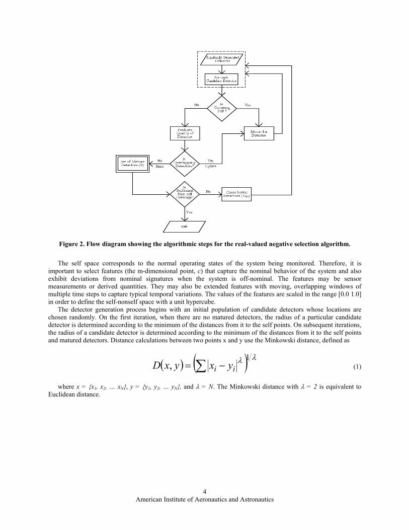
There are two phases in immunity-based fault detection, detector generation and testing. In the detector

generation phase, the RNS algorithm evolves a set of variable-size detectors that cover the non-self space. A detector is defined as d = (c, rd), where c = (c1, c2, …, cm) is an m-dimensional point that corresponds to the center of a hypersphere with radius rd. An iterative process, shown in Fig. 2, updates the set of detectors by random generation, moving a subset of rejected detectors that overlap self or other detectors, and cloning a subset of the matured detectors.


4

Figure 2. Flow diagram showing the algorithmic steps for the real-valued negative selection algorithm.

The self space corresponds to the normal operating states of the system being monitored. Therefore, it is

important to select features (the m-dimensional point, c) that capture the nominal behavior of the system and also exhibit deviations from nominal signatures when the system is off-nominal. The features may be sensor measurements or derived quantities. They may also be extended features with moving, overlapping windows of multiple time steps to capture typical temporal variations. The values of the features are scaled in the range [0.0 1.0] in order to define the self-nonself space with a unit hypercube.

The detector generation process begins with an initial population of candidate detectors whose locations are chosen randomly. On the first iteration, when there are no matured detectors, the radius of a particular candidate detector is determined according to the minimum of the distances from it to the self points. On subsequent iterations, the radius of a candidate detector is determined according to the minimum of the distances from it to the self points and matured detectors. Distance calculations between two points x and y use the Minkowski distance, defined as

( ) ( ) λλ 1, ∑ −= ii yxyxD (1)

where x = {x1, x2, … xN}, y = {y1, y2, … yN}, and λ = N. The Minkowski distance with λ = 2 is equivalent to Euclidean distance.


5

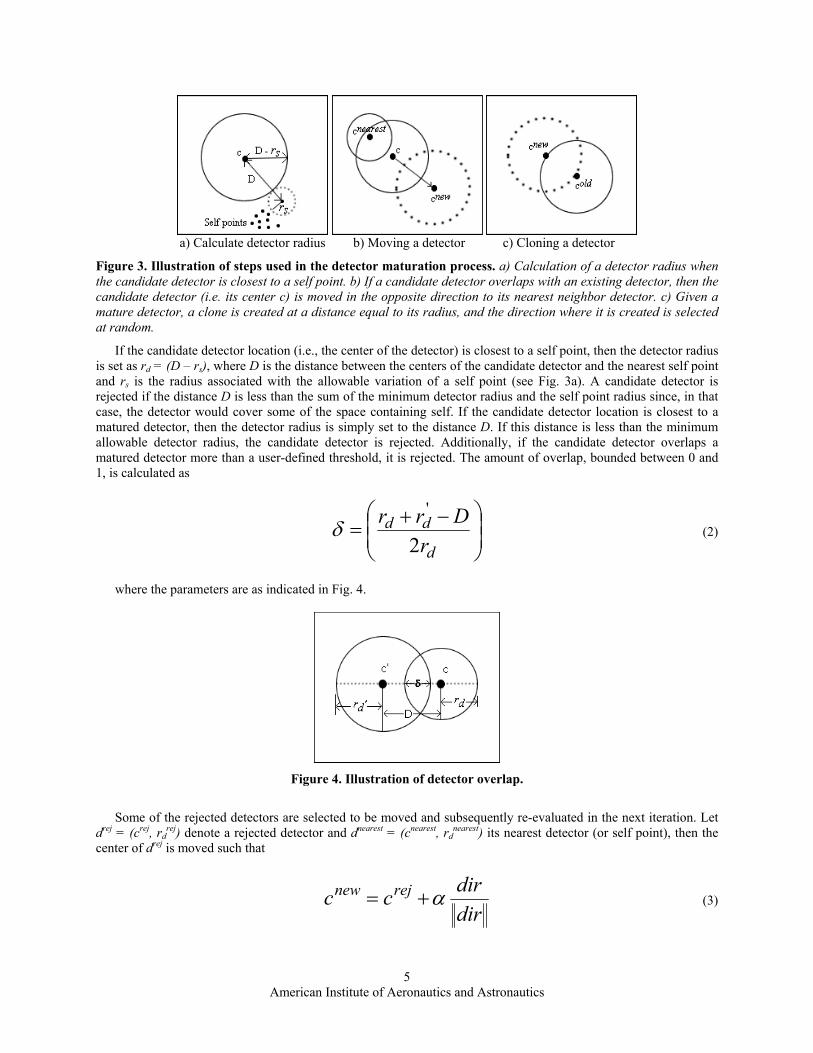
a) Calculate detector radius b) Moving a detector c) Cloning a detector

Figure 3. Illustration of steps used in the detector maturation process. a) Calculation of a detector radius when the candidate detector is closest to a self point. b) If a candidate detector overlaps with an existing detector, then the candidate detector (i.e. its center c) is moved in the opposite direction to its nearest neighbor detector. c) Given a mature detector, a clone is created at a distance equal to its radius, and the direction where it is created is selected at random.

If the candidate detector location (i.e., the center of the detector) is closest to a self point, then the detector radius is set as rd = (D – rs), where D is the distance between the centers of the candidate detector and the nearest self point and rs is the radius associated with the allowable variation of a self point (see Fig. 3a). A candidate detector is rejected if the distance D is less than the sum of the minimum detector radius and the self point radius since, in that case, the detector would cover some of the space containing self. If the candidate detector location is closest to a matured detector, then the detector radius is simply set to the distance D. If this distance is less than the minimum allowable detector radius, the candidate detector is rejected. Additionally, if the candidate detector overlaps a matured detector more than a user-defined threshold, it is rejected. The amount of overlap, bounded between 0 and 1, is calculated as

−+=

d

ddr

Drr2

'δ (2)

where the parameters are as indicated in Fig. 4.

Figure 4. Illustration of detector overlap.

Some of the rejected detectors are selected to be moved and subsequently re-evaluated in the next iteration. Let

drej = (crej, rdrej) denote a rejected detector and dnearest = (cnearest, rd

nearest) its nearest detector (or self point), then the center of drej is moved such that

dirdircc rejnew α+= (3)


6

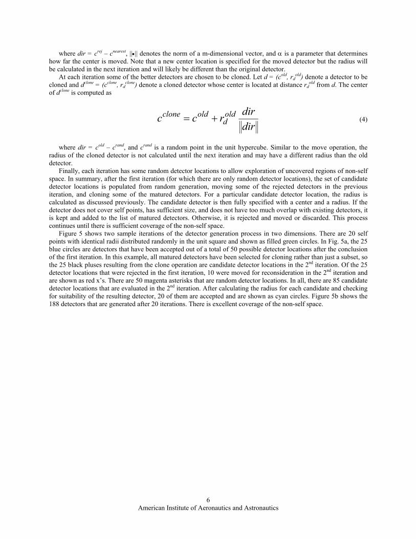
where dir = crej – cnearest, ||•|| denotes the norm of a m-dimensional vector, and α is a parameter that determines how far the center is moved. Note that a new center location is specified for the moved detector but the radius will be calculated in the next iteration and will likely be different than the original detector.

At each iteration some of the better detectors are chosen to be cloned. Let d = (cold, rdold) denote a detector to be

cloned and dclone = (cclone, rdclone) denote a cloned detector whose center is located at distance rd

old from d. The center of dclone is computed as

dirdirrcc old

doldclone += (4)

where dir = cold – crand, and crand is a random point in the unit hypercube. Similar to the move operation, the radius of the cloned detector is not calculated until the next iteration and may have a different radius than the old detector.

Finally, each iteration has some random detector locations to allow exploration of uncovered regions of non-self space. In summary, after the first iteration (for which there are only random detector locations), the set of candidate detector locations is populated from random generation, moving some of the rejected detectors in the previous iteration, and cloning some of the matured detectors. For a particular candidate detector location, the radius is calculated as discussed previously. The candidate detector is then fully specified with a center and a radius. If the detector does not cover self points, has sufficient size, and does not have too much overlap with existing detectors, it is kept and added to the list of matured detectors. Otherwise, it is rejected and moved or discarded. This process continues until there is sufficient coverage of the non-self space.

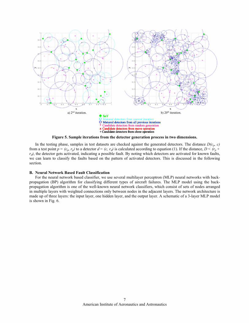
Figure 5 shows two sample iterations of the detector generation process in two dimensions. There are 20 self points with identical radii distributed randomly in the unit square and shown as filled green circles. In Fig. 5a, the 25 blue circles are detectors that have been accepted out of a total of 50 possible detector locations after the conclusion of the first iteration. In this example, all matured detectors have been selected for cloning rather than just a subset, so the 25 black pluses resulting from the clone operation are candidate detector locations in the 2nd iteration. Of the 25 detector locations that were rejected in the first iteration, 10 were moved for reconsideration in the 2nd iteration and are shown as red x’s. There are 50 magenta asterisks that are random detector locations. In all, there are 85 candidate detector locations that are evaluated in the 2nd iteration. After calculating the radius for each candidate and checking for suitability of the resulting detector, 20 of them are accepted and are shown as cyan circles. Figure 5b shows the 188 detectors that are generated after 20 iterations. There is excellent coverage of the non-self space.


7

x x

y y

Matured detectors from all previous iterations

x Candidate detectors from move operation

SelfMatured detectors from current iteration

* Candidate detectors from random generation

+ Candidate detectors from clone operation

a) 2nd iteration. b) 20th iteration.x x

y y











a) 2nd iteration. b) 20th iteration.

Figure 5. Sample iterations from the detector generation process in two dimensions.

In the testing phase, samples in test datasets are checked against the generated detectors. The distance D(cp, c) from a test point p = (cp, rp) to a detector d = (c, rd) is calculated according to equation (1). If the distance, D < (rp + rd), the detector gets activated, indicating a possible fault. By noting which detectors are activated for known faults, we can learn to classify the faults based on the pattern of activated detectors. This is discussed in the following section.

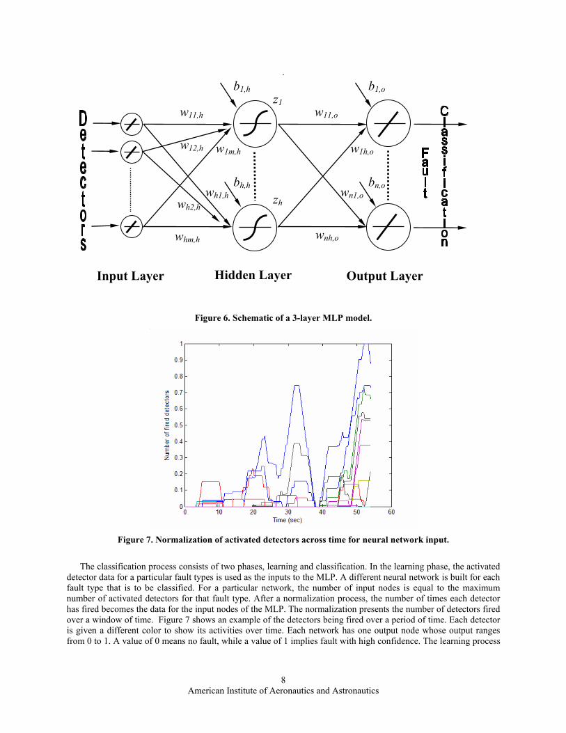
B. Neural Network Based Fault Classification For the neural network based classifier, we use several multilayer perceptron (MLP) neural networks with back-

propagation (BP) algorithm for classifying different types of aircraft failures. The MLP model using the back-propagation algorithm is one of the well-known neural network classifiers, which consist of sets of nodes arranged in multiple layers with weighted connections only between nodes in the adjacent layers. The network architecture is made up of three layers: the input layer, one hidden layer, and the output layer. A schematic of a 3-layer MLP model is shown in Fig. 6.


8

.

Figure 6. Schematic of a 3-layer MLP model.

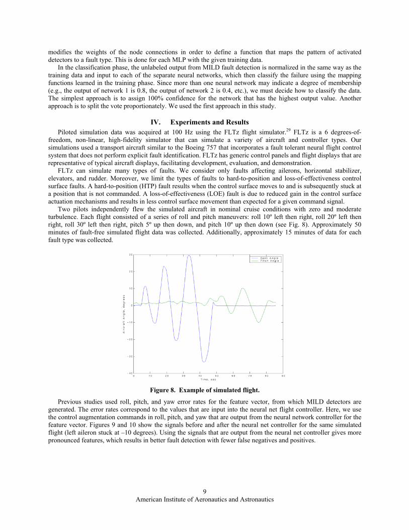
Figure 7. Normalization of activated detectors across time for neural network input.

The classification process consists of two phases, learning and classification. In the learning phase, the activated

detector data for a particular fault types is used as the inputs to the MLP. A different neural network is built for each fault type that is to be classified. For a particular network, the number of input nodes is equal to the maximum number of activated detectors for that fault type. After a normalization process, the number of times each detector has fired becomes the data for the input nodes of the MLP. The normalization presents the number of detectors fired over a window of time. Figure 7 shows an example of the detectors being fired over a period of time. Each detector is given a different color to show its activities over time. Each network has one output node whose output ranges from 0 to 1. A value of 0 means no fault, while a value of 1 implies fault with high confidence. The learning process

b1,h

bh,h

w11,h

whm,h

w1m,hw12,h

wh1,hwh2,h

z1

zh

b1,o

bn,o

w11,o

wnh,o

w1h,o

wn1,o

Input Layer Hidden Layer Output Layer


9

modifies the weights of the node connections in order to define a function that maps the pattern of activated detectors to a fault type. This is done for each MLP with the given training data.

In the classification phase, the unlabeled output from MILD fault detection is normalized in the same way as the training data and input to each of the separate neural networks, which then classify the failure using the mapping functions learned in the training phase. Since more than one neural network may indicate a degree of membership (e.g., the output of network 1 is 0.8, the output of network 2 is 0.4, etc.), we must decide how to classify the data. The simplest approach is to assign 100% confidence for the network that has the highest output value. Another approach is to split the vote proportionately. We used the first approach in this study.

IV. Experiments and Results Piloted simulation data was acquired at 100 Hz using the FLTz flight simulator.29 FLTz is a 6 degrees-of-

freedom, non-linear, high-fidelity simulator that can simulate a variety of aircraft and controller types. Our simulations used a transport aircraft similar to the Boeing 757 that incorporates a fault tolerant neural flight control system that does not perform explicit fault identification. FLTz has generic control panels and flight displays that are representative of typical aircraft displays, facilitating development, evaluation, and demonstration.

FLTz can simulate many types of faults. We consider only faults affecting ailerons, horizontal stabilizer, elevators, and rudder. Moreover, we limit the types of faults to hard-to-position and loss-of-effectiveness control surface faults. A hard-to-position (HTP) fault results when the control surface moves to and is subsequently stuck at a position that is not commanded. A loss-of-effectiveness (LOE) fault is due to reduced gain in the control surface actuation mechanisms and results in less control surface movement than expected for a given command signal.

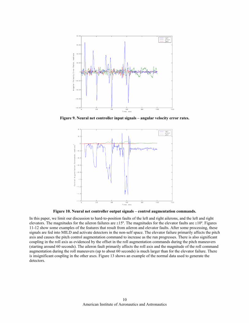
Two pilots independently flew the simulated aircraft in nominal cruise conditions with zero and moderate turbulence. Each flight consisted of a series of roll and pitch maneuvers: roll 10º left then right, roll 20º left then right, roll 30º left then right, pitch 5º up then down, and pitch 10º up then down (see Fig. 8). Approximately 50 minutes of fault-free simulated flight data was collected. Additionally, approximately 15 minutes of data for each fault type was collected.

Figure 8. Example of simulated flight.

Previous studies used roll, pitch, and yaw error rates for the feature vector, from which MILD detectors are generated. The error rates correspond to the values that are input into the neural net flight controller. Here, we use the control augmentation commands in roll, pitch, and yaw that are output from the neural network controller for the feature vector. Figures 9 and 10 show the signals before and after the neural net controller for the same simulated flight (left aileron stuck at –10 degrees). Using the signals that are output from the neural net controller gives more pronounced features, which results in better fault detection with fewer false negatives and positives.


10

Figure 9. Neural net controller input signals – angular velocity error rates.

Figure 10. Neural net controller output signals – control augmentation commands.

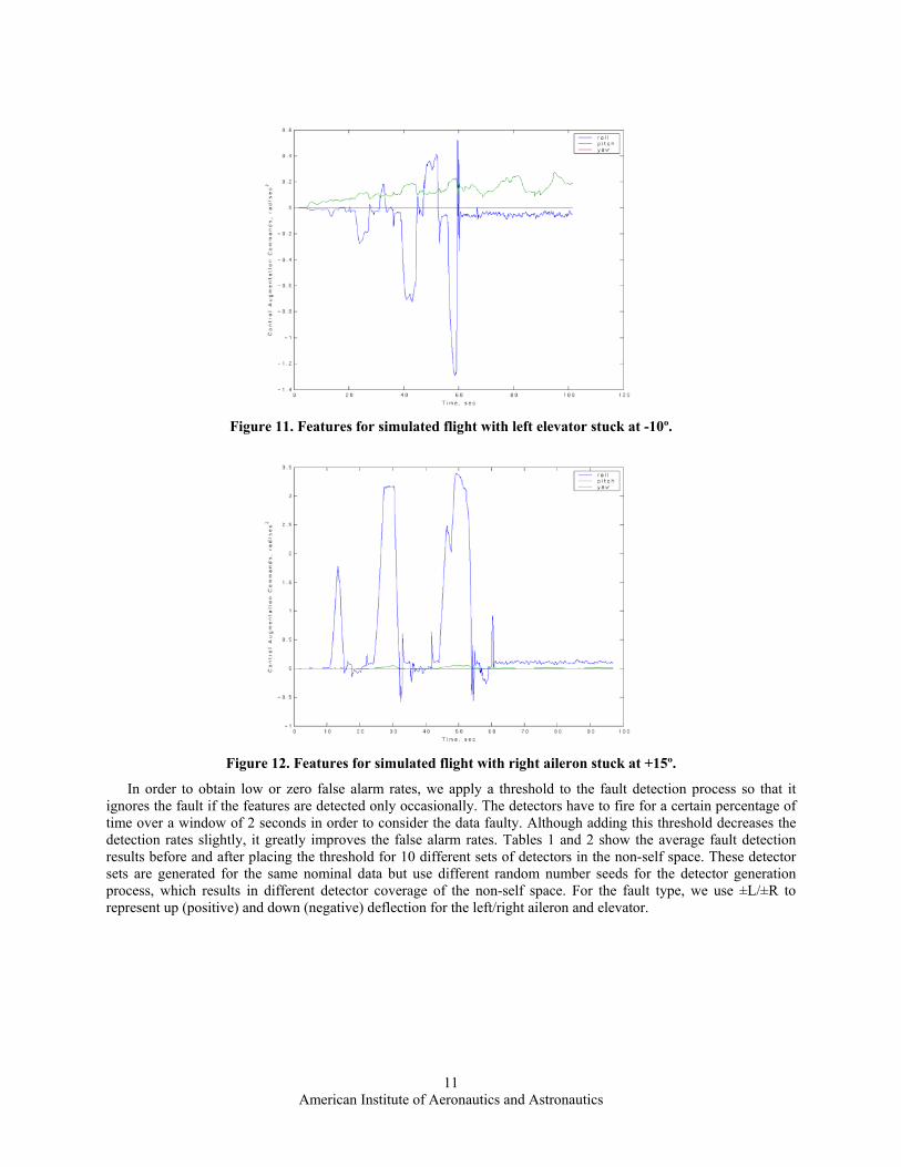
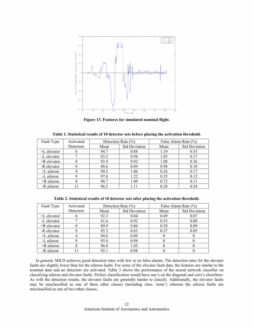
In this paper, we limit our discussion to hard-to-position faults of the left and right ailerons, and the left and right elevators. The magnitudes for the aileron failures are ±15º. The magnitudes for the elevator faults are ±10º. Figures 11-12 show some examples of the features that result from aileron and elevator faults. After some processing, these signals are fed into MILD and activate detectors in the non-self space. The elevator failure primarily affects the pitch axis and causes the pitch control augmentation command to increase as the run progresses. There is also significant coupling in the roll axis as evidenced by the offset in the roll augmentation commands during the pitch maneuvers (starting around 60 seconds). The aileron fault primarily affects the roll axis and the magnitude of the roll command augmentation during the roll maneuvers (up to about 60 seconds) is much larger than for the elevator failure. There is insignificant coupling in the other axes. Figure 13 shows an example of the normal data used to generate the detectors.


11

Figure 11. Features for simulated flight with left elevator stuck at -10º.

Figure 12. Features for simulated flight with right aileron stuck at +15º.

In order to obtain low or zero false alarm rates, we apply a threshold to the fault detection process so that it ignores the fault if the features are detected only occasionally. The detectors have to fire for a certain percentage of time over a window of 2 seconds in order to consider the data faulty. Although adding this threshold decreases the detection rates slightly, it greatly improves the false alarm rates. Tables 1 and 2 show the average fault detection results before and after placing the threshold for 10 different sets of detectors in the non-self space. These detector sets are generated for the same nominal data but use different random number seeds for the detector generation process, which results in different detector coverage of the non-self space. For the fault type, we use ±L/±R to represent up (positive) and down (negative) deflection for the left/right aileron and elevator.


12

Figure 13. Features for simulated nominal flight.

Table 1. Statistical results of 10 detector sets before placing the activation threshold.

Detection Rate (%) False Alarm Rate (%) Fault Type Activated Detectors Mean Std Deviation Mean Std Deviation

+L elevator 6 94.7 0.88 1.19 0.53 -L elevator 7 83.2 0.94 1.03 0.17 +R elevator 8 92.9 0.92 1.08 0.36 -R elevator 9 88.6 0.89 0.98 0.18 +L aileron 4 99.5 1.06 0.26 0.17 -L aileron 9 97.8 1.22 0.35 0.12 +R aileron 8 98.7 1.09 0.72 0.11 -R aileron 11 96.2 1.11 0.28 0.24

Table 2. Statistical results of 10 detector sets after placing the activation threshold.

Detection Rate (%) False Alarm Rate (%) Fault Type Activated Detectors Mean Std Deviation Mean Std Deviation

+L elevator 6 92.3 0.84 0.49 0.07 -L elevator 7 81.6 0.92 0.53 0.08 +R elevator 8 89.9 0.86 0.38 0.09 -R elevator 9 85.3 0.83 0.37 0.05 +L aileron 4 94.6 0.89 0 0 -L aileron 9 93.4 0.98 0 0 +R aileron 8 96.8 1.03 0 0 -R aileron 11 92.1 0.98 0 0

In general, MILD achieves good detection rates with few or no false alarms. The detection rates for the elevator

faults are slightly lower than for the aileron faults. For some of the elevator fault data, the features are similar to the nominal data and no detectors are activated. Table 3 shows the performance of the neural network classifier on classifying aileron and elevator faults. Perfect classification would have one’s on the diagonal and zero’s elsewhere. As with the detection results, the elevator faults are generally harder to classify. Additionally, the elevator faults may be misclassified as one of three other classes (including class ‘none’) whereas the aileron faults are misclassified as one of two other classes.


13

Table 3. Performance of neural network classifier on classifying aileron and elevator faults.

NONE

+L

elevator -L

elevator

+R

elevator -R

elevator +L

aileron -L

aileron +R

aileron -R

aileron

NONE 1 0 0 0 0 0 0 0 0 +L elevator 0.08 0.82 0.02 0 0.08 0 0 0 0 -L elevator 0.11 0.04 0.79 0.06 0 0 0 0 0 +R elevator 0.06 0 0.07 0.84 0.03 0 0 0 0 -R elevator 0.02 0.07 0.03 0 0.88 0 0 0 0 +L aileron 0.02 0 0 0 0 0.92 0 0.06 0 -L aileron 0.04 0 0 0 0 0 0.89 0 0.07 +R aileron 0.07 0 0 0 0 0.11 0 0.82 0 -R aileron 0.02 0 0 0 0 0 0.04 0 0.92

V. Conclusions Previous work has shown that MILD is an effective tool for detecting aircraft faults. In this work, we have

improved on previous detection results by using the output of the neural network instead of the input and have demonstrated a MILD add-on: a neural-network fault classifier, which is able to classify different types of faults based on the pattern of detectors that are activated. Together, the fault detector and classifier provide a means to improve the pilot’s situational awareness of aircraft faults that may be masked by the neural net flight controller. MILD output may also be used in the feedback control loop to improve aircraft handling qualities under failures.

Further areas for research include extending the analysis to other flight regimes such as approach to landing, investigating the sensitivity of the detection and classification results to different pilots, and examining other classification techniques. For MILD, we will explore how we can further optimize the detector generation phase to reduce the training and fault detection time. Furthermore, we plan to examine higher order detector shapes and the concept of a gene library to enrich the detection process.

Acknowledgments Derek Wong was funded by the NASA Ames Educator Associate’s Program. We thank pilots Don Bryant and

Scott Christa for flying the simulator.

References 1Araujo, M., Aguilar, J., and Aponte, H., “Fault detection system in gas lift well based on Artificial Immune System,”

Proceedings of the International Joint Conference on AI, pp. 1673 -1677, No. 3, July 20 - 24, 2003. 2Boskovic, J. D., and Mehra, R. K., “Intelligent Adaptive Control of a Tailless Advanced Fighter Aircraft under Wing

Damage,” Journal of Guidance, Control, and Dynamics (American Institute of Aeronautics and Astronautics), Year: 2000 Volume: 23 Number: 5 Pages: 876-884.

3Boskovic, J. D., and Mehra, R. K., “Multiple-Model Adaptive Flight Control Scheme for Accommodation of Actuator Failures,” Journal of Guidance, Control, and Dynamics (American Institute of Aeronautics and Astronautics), 2002 Volume: 25 Number: 4 Pages: 712-724.

4Bradley, D., and Tyrrell, A., “Hardware Fault Tolerance: An Immunological Solution,” Proceedings of IEEE International Conference on Systems, Man and Cybernetics (SMC), Nashville, October 8-11, 2000.

5Brinker, J. S., and Wise, K. A., “Flight Testing of Reconfigurable Control Law on the X-36 Tailless Aircraft,” Journal of Guidance, Control, and Dynamics (American Institute of Aeronautics and Astronautics) Year: 2001 Volume: 24 Number: 5 Pages: 903-909.

6Chen, Y. M., and Lee, M. L., “Neural networks-based scheme for system failure detection and diagnosis,” Mathematics and Computers in Simulation (Elsevier Science), Year: 2002 Volume: 58 Number: 2 Pages: 101-109.

7Dasgupta, D., and Forrest, S., “An anomaly detection algorithm inspired by the immune system,” Artificial Immune Systems and Their Applications, edited by D. Dasgupta, Springer-Verlag, 1999, pp.262–277.

8Dasgupta, D., KrishnaKumar, K., Wong, D., and Berry, M., “Immunity-Based Aircraft Fault Detection System,” Proceedings of American Institute of Aeronautics and Astronautics Chicago, USA September 20-24, 2004.

9Dasgupta, D., “An Overview of Artificial Immune Systems and Their Applications”, Artificial Immune Systems and Their Applications, edited by D. Dasgupta, Berlin: Springer-Verlag, 1998, pp. 3-21.


14

10D’haeseleer, P., Forrest, S., and Helman, P., “An immunological approach to change detection: algorithms, analysis, and implications,” Proceedings of the IEEE Symposium on Computer Security and Privacy, IEEE Computer Society Press, Los Alamitos, CA, 1996, pp. 110–119.

11Forrest, S., Perelson, A. S., Allen, L., and Cherukuri, R., “Self-nonself discrimination in a computer,” Proceedings of the IEEE Symposium on Research in Security and Privacy, IEEE Computer Society Press, Los Alamitos, CA, 1994, pp. 202–212.

12Gonzales, F., and Dasgupta, D., “Anomaly Detection Using Real-Valued Negative Selection,” Genetic Programming and Evolvable Machines, 4, 2003, pp. 383-403.

13Gundy-Burlet, K., Krishnakumar, K., Limes, G., and Bryant, D., “Control Reallocation Strategies for Damage Adaptation in Transport Class Aircraft,” AIAA 2003-5642, August, 2003.

14KrishnaKumar, K., “Artificial Immune System Approaches for Aerospace Applications,” American Institute of Aeronautics and Astronautics 41st Aerospace Sciences Meeting and Exhibit, Reno, Nevada, 6-9 January 2003.

15KrishnaKumar, K., Limes, G., Gundy-Burlet, K., and Bryant, D., “An Adaptive Critic Approach to Reference Model Adaptation,” AIAA GN&C Conf. 2003.

16Niño, F., Gómez, D., and Vejar, R., “A Novel Immune Anomaly Detection Technique Based on Negative Selection,” Proceedings of the Genetic and Evolutionary Computation Conference (GECCO) [Poster], Chicago, IL, USA, July 12-16, 2003. LNCS 2723, p. 243.

17Pachter, M., and Huang, Y., “Fault Tolerant Flight Control,” Journal of Guidance, Control, and Dynamics (American Institute of Aeronautics and Astronautics) Year: 2003 Volume: 26 Number: 1 Pages: 151-160.

18Rysdyk, R. T., and Calise, A. J., “Fault Tolerant Flight Control via Adaptive Neural Network Augmentation,” AIAA 98-4483, August 1998.

19Shulin, L., Jiazhong, Z., Wengang, S., and Wenhu, H., “Negative-selection algorithm based approach for fault diagnosis of rotary machinery,” Proceedings of American Control Conference, 2002, Vol. 5, pp. 3955 -3960. 8-10 May 8-10, 2002.

20Singh, S., “Anomaly detection using negative selection based on the r-contiguous matching rule,” 1st International Conference on Artificial Immune Systems (ICARIS), University of Kent at Canterbury, UK, September 9th-11th, 2002.

21Taylor, D. W., and Corne, D. W., “An Investigation of the Negative Selection Algorithm for Fault Detection in Refrigeration Systems,” Proceeding of Second International Conference on Artificial Immune Systems (ICARIS), September 1-3, 2003, Napier Uni.,Edinburgh, UK.

22Xanthakis, S., Karapoulios, S., Pajot, R., and Rozz, A., “Immune System and Fault Tolerant Computing,” In J.M. Alliot, editor, Artificial Evolution, volume 1063 of Lecture Notes in Computer Science, pages 181-197. Springer-Verlag, 1996.

23McCelland, J. L., and Rumelhar, D. E., Eds., Parallel Distributed Processing, Vol. 1. Cambridge, MA : MIT Press, 1986. 24Pao, Y. H., Adaptive pattern Recognition and Neural Network, Addition-Wesley Publishing Company, Inc., 1989. 25Bendiktsson, J. A., Swain, P. H., and Ersoy, O. K., "Neural Network Approaches Versus Statistical Methods on

Classification of Multisource Remote Sensing Data", IEEE Trans. Geosci. Remote Sensing, vol. 28, pp. 540-552, July 1990. 26Bichof, H., Schneider, W., and Pinz, A. J., "Multishpectral Classification of Landsat Image using Neural Networks", IEEE

Trans. Geosci. Remote Sensing. Vol. 30, pp. 482-480, May 1992. 27Heermann, P. D., and Khozenie, N., "Classification of Multispectral Remote Sensing Data Using a Back-propagation

Neural Network", IEEE Trans. Geosci, Remote Sensing, vol. 30, pp. 81-88; Jan. 1992. 28Annema, A. J., Feed-Forward Neural Network : Vector Decomposition Analysis Modeling and Analog Implementation,

Kluwer Academic Publishers , 1995. 29Kaneshige, J., Bull, J., and Totah, J., “Generic Neural Flight Control and Autopilot System,” AIAA Journal 4281, 2000.

aircraft fault detection and classification using multi ... (wong).pdf · aircraft fault detection...

Documents