AIRFOIL BOUNDARY LAYER CALCULATIONS USING INTERACTIVE METHOD AND en TRANSITION PREDICTION

TECHNIQUE

MEHMET MERSİNLİGİL

SEPTEMBER 2006

AIRFOIL BOUNDARY LAYER CALCULATIONS USING INTERACTIVE METHOD AND en TRANSITION PREDICTION

TECHNIQUE

A THESIS SUBMITTED TO THE GRADUATE SCHOOL OF NATURAL AND APPLIED SCIENCES

OF MIDDLE EAST TECHNICAL UNIVERSITY

BY

MEHMET MERSİNLİGİL

IN PARTIAL FULFILLMENT OF THE REQUIREMENTS FOR

THE DEGREE OF MASTER OF SCIENCE IN

AEROSPACE ENGINEERING

SEPTEMBER 2006

Approval of the Graduate School of Natural and Applied Sciences

________________________ Prof. Dr. Canan Özgen Director

I certify that this thesis satisfies all the requirements as a thesis for the degree of Master of

Science

________________________ Prof. Dr. Nafiz Alemdaroğlu Head of the Department

We certify that we have read this thesis and in our opinion it is fully adequate, in scope

and quality, as a thesis for the degree of Master of Science in Aerospace Engineering.

________________________ Assoc. Prof. Dr. Serkan Özgen Supervisor

Prof. Dr. Nafiz Alemdaroğlu METU, AE ________________________

Prof. Dr. Zafer Dursunkaya METU, ME ________________________

Prof. Dr. Yusuf Özyörük METU, AE ________________________

Assoc. Prof. Dr. Serkan Özgen METU, AE ________________________

Dr. Oğuz Uzol METU, AE ________________________

iii

PLAGIARISM

I hereby declare that all information in this document has been obtained and presented in

accordance with academic rules and ethical conduct. I also declare that, as required by

these rules and conduct, I have fully cited and referenced all material and results that are

not original to this work.

Mehmet Mersinligil

iv

A B S T R A C T

AIRFOIL BOUNDARY LAYER CALCULATIONS USING INTERACTIVE METHOD AND en TRANSITION PREDICTION TECHNIQUE

MERSİNLİGİL, Mehmet

M.S., Department of Aerospace Engineering

Supervisor: Assoc. Prof. Dr. Serkan Özgen

September, 2006, 102 pages

Boundary layer calculations are performed around an airfoil and its wake. Smith-van Ingen

transition prediction method is employed to find the transition from laminar to turbulent

flow. First, potential flow around the airfoil is solved with the Hess-Smith panel method.

The resulting velocity distribution is input to the boundary layer equations in order to find

a so called blowing velocity distribution. The output of the boundary layer equations are

also used to compute the location of onset of transition using the Smith-van Ingen en

transition prediction method. The obtained blowing velocity distribution is fed back to the

panel method to find a velocity distribution which includes the effects of viscosity. The

procedure described is repeated until convergence is observed. A computer program is

developed using the theory. Results obtained are in good accord with measurements.

Keywords : Boundary Layer Flows, Transition Prediction, Blowing Velocity, Airfoil Performance, Interactive Method

Science Code : 618.01.01

v

Ö Z

KANAT PROFİLİ SINIR TABAKASININ ETKİLEŞİMLİ METOD VE en GEÇİŞ TAHMİN TEKNİĞİ KULLANILARAK HESAPLANMASI

MERSİNLİGİL, Mehmet

Yüksek Lisans, Havacılık ve Uzay Mühendisliği Anabilim Dalı

Tez Danışmanı: Doç. Dr. Serkan Özgen

Eylül, 2006, 102 sayfa

Kanat profili ve ard iz bölgesinde sınır tabakası hesaplamaları yapılmıştır. Geçiş tahmini

için Smith-van Ingen geçiş tahmin metodu kullanılmıştır. İlk önce Hess-Smith panel

metodu kullanılarak kanat profili etrafındaki potansiyel akım çözülmüş ve hız dağılımı

hesaplanmıştır. Elde edilen hız dağılımı ile sınır tabakası denklemleri çözülmüş ve yüzey

üfleme hızları bulunmuştur. Sınır tabakası denklemlerinin sonuçları, Smith-van Ingen en

metodu ile türbülansa geçiş noktasının belirlenmesi için kullanılmıştır. Elde edilen yüzey

üfleme hızları potansiyel akım çözümünde sınır şartları olarak kullanılmış ve sınır

tabakasının etkilerini de içeren potansiyel akım bulunmuştur. Bu yöntem, yakınsama

gözlemleninceye değin sürdürülmüştür. Söz konusu teori kullanılarak bir bilgisayar

programı yazılmış ve iki adet kanat profili etrafında denenmiştir. Sonuçlar deneysel

ölçümler ile uyumludur.

Anahtar Kelimeler : Sınır Tabaka Akışı, Geçiş Tahmini, Yüzey Üfleme Hızı, Kanat Profili Performansı, Etkileşimli Yöntem

Bilim Dalı Sayısal Kodu : 618.01.01

vi

DEDICATION

To my family, without whom this study would be impossible…

vii

A C K N O W L E D G M E N T S

The author wishes to thank to Associate Professor Serkan Özgen for his precious

guidance and sincere efforts which enabled this study to be done.

viii

T A B L E O F C O N T E N T S

PLAGIARISM....................................................................................................................................iii ABSTRACT ....................................................................................................................................... iv ÖZ......................................................................................................................................................... v DEDICATION................................................................................................................................. vi ACKNOWLEDGMENTS............................................................................................................ vii TABLE OF CONTENTS ............................................................................................................ viii LIST OF FIGURES......................................................................................................................... ix CHAPTERS

1 INTRODUCTION ................................................................................................................ 1 2 BOUNDARY LAYER EQUATIONS FOR 2D FLOWS............................................ 6

2.1 Continuity Equation...................................................................................................... 6 2.2 Momentum Equation ................................................................................................... 7 2.3 Boundary Layer Equations .......................................................................................... 9

3 SOLUTION OF 2D BOUNDARY LAYER EQUATIONS..................................... 13 3.1 Interaction Mechanism between Inviscid and Viscous Solutions...................... 14 3.2 Solution of the Standard Problem............................................................................ 17 3.3 Inverse Problem........................................................................................................... 27 3.4 Solution Procedure for the Wake Region ............................................................... 34

4 TRANSITION METHOD IN 2D INCOMPRESSIBLE FLOWS .......................... 37 4.1 Smith-van Ingen en Procedure .................................................................................. 41 4.2 Numerical Scheme ...................................................................................................... 43 4.3 Calculation of the Neutral Stability Curve and the Dimensional Frequencies 48 4.4 Calculating the Onset of Transition......................................................................... 53

5 TURBULENCE MODEL.................................................................................................. 55 5.1 Turbulence Model Used for the Boundary Layer ................................................. 55 5.2 Turbulence Model Used for the Wake Region...................................................... 60

6 RESULTS AND DISCUSSION........................................................................................ 61 6.1 Falkner Skan Flow....................................................................................................... 63 6.2 Airfoil Flow................................................................................................................... 70

7 CONCLUSION..................................................................................................................... 81 BIBLIOGRAPHY........................................................................................................................... 83 APPENDICES

A BLOCK ELIMINATION METHOD............................................................................ 86 A.1. Forward Sweep .......................................................................................................... 87 A.2. Backward Sweep ........................................................................................................ 89

B APPROXIMATION OF THE HILBERT INTEGRAL ........................................... 90 C DERIVATION OF THE ORR-SOMMERFELD EQUATION ............................ 94

C.1. Reduction to a fourth order system ....................................................................... 98 C.2. Special Form of the Stability Equations: Orr-Sommerfeld Equation.............. 99

D DESCRIPTION OF THE COMPUTER PROGRAM............................................ 101

ix

L I S T O F F I G U R E S

Number Page

Figure 1.1 Brief Flowchart of the Solution Procedure............................................................... 3 Figure 3.1 Definition of Displacement Thickness.................................................................... 16 Figure 3.2 Rectangular grid used for centered difference approximation............................ 20 Figure 4.1 Schematic of transition calculation using en method ............................................ 42 Figure 4.2 Change in integrated amplification factor with respect to distance for

Blasius Flow ........................................................................................................................ 43 Figure 6.1 Convergence history for NACA 0012 Airfoil ( cR =6×106, α =12 ° )............... 62 Figure 6.2 Neutral Stability Curve for Blasius Flow................................................................. 64 Figure 6.3 Change in integrated amplification factor with respect to distance for

Falkner Skan Flow with β =-0.1988.............................................................................. 64 Figure 6.4 Change in integrated amplification factor with respect to distance for

Falkner Skan Flow with β =-0.15 .................................................................................. 65 Figure 6.5 Change in integrated amplification factor with respect to distance for

Falkner Skan Flow with β =-0.1 .................................................................................... 65 Figure 6.6 Change in integrated amplification factor with respect to distance for

Falkner Skan Flow with β =-0.05 .................................................................................. 66 Figure 6.7 Change in integrated amplification factor with respect to distance for

Blasius Flow ........................................................................................................................ 66 Figure 6.8 Change in integrated amplification factor with respect to distance for

Falkner Skan Flow with β =0.05.................................................................................... 67 Figure 6.9 Change in integrated amplification factor with respect to distance for

Falkner Skan Flow with β =0.1...................................................................................... 67 Figure 6.10 Change in integrated amplification factor with respect to distance for

Falkner Skan Flow with β =0.2...................................................................................... 68 Figure 6.11 Change in integrated amplification factor with respect to distance for

Falkner Skan Flow with β =0.3...................................................................................... 68 Figure 6.12 Change in integrated amplification factor with respect to distance for

Falkner Skan Flow with β =0.4...................................................................................... 69 Figure 6.13 Change in integrated amplification factor with respect to distance for

Falkner Skan Flow with β =0.5...................................................................................... 69 Figure 6.14 Variation of lift coefficient with respect to angle of attack for NACA 0012

airfoil for cR =2×105 and cR =6×106............................................................................ 70 Figure 6.15 Amplification rates calculated using the en method for lower surface of

NACA 0012 Airfoil at cR =6×106 and α =4° ............................................................ 72 Figure 6.16 Variation of drag coefficient with respect to lift coefficient for NACA

0012 airfoil for cR =2×105 and cR =6×106 .................................................................. 73 Figure 6.17 Variation of the displacement thickness with respect to angle of attack for

NACA 0012 airfoil for cR =6×106................................................................................. 74 Figure 6.18 Inviscid and viscous pressure distribution around NACA 0012 airfoil for

cR =6×106 at α =14° ...................................................................................................... 74

x

Figure 6.19 Displacement thickness distribution at the upper surface of NACA 0012 airfoil and its wake for cR =6×106 and α =10° ......................................................... 75

Figure 6.20 Selected velocity profiles at the upper surface of NACA 0012 airfoil for cR =6×106 and α =15° ................................................................................................... 75

Figure 6.21 Velocity profiles in the wake for NACA 0012 airfoil for cR =6×106 and α =0° .................................................................................................................................. 76

Figure 6.22 Velocity profiles in the wake for NACA 0012 airfoil for cR =6×106 and α =8° .................................................................................................................................. 77

Figure 6.23 Velocity profiles in the wake for NACA 0012 airfoil for cR =6×106 and α =15° ................................................................................................................................ 77

Figure 6.24 Variation of drag surface friction coefficient against surface distance traversed for NACA 0012 airfoil for cR =2×105......................................................... 78

Figure 6.25 Variation of lift coefficient with respect to angle of attack for NACA 4412 airfoil for cR =2×105 and cR =6×106............................................................................ 79

Figure 6.26 Variation of drag coefficient with respect to lift coefficient for NACA 4412 airfoil for cR =2×105 and cR =6×106 .................................................................. 80

Figure 6.27 Variation of drag surface friction coefficient against surface distance traversed for NACA 4412 airfoil for cR =2×105......................................................... 80

1

C H A P T E R 1

INTRODUCTION

As lifting sections play an essential role in performance of any aerodynamic system, two

questions are of particular importance. First is the problem of designing lifting sections,

where the second is to analyze performance characteristics. Analysis of lifting sections is

crucial from design of an airfoil to design of an aircraft.

In order to analyze a lifting section, mainly two approaches are applicable. One is to solve

either full Navier-Stokes (N-S) equations or to solve them in a simplified manner, which is

called the thin-layer Navier-Stokes equations, where diffusion terms in the mean flow

direction are neglected. The main complexity of the so called thin layer Navier-Stokes

equations arise from the fact that, the whole flow field has to be treated simultaneously,

since these equations are not parabolic in nature and therefore does not allow one to use

techniques such as marching technique. Obviously, since one has to handle the whole

flow field at once, this method requires some large amount of computational power and

storage space, which makes it unfeasible.

An alternative method is the so called Interactive Boundary Layer method. In this

method, the major assumption is the one suggested by Prandtl, which implies that for

sufficiently high Reynolds numbers, flow over a lifting section can be considered as

superposition of two different layers, a thin boundary layer, or viscous layer, where all the

viscous effects are included, and an inviscid outer layer. As stated in [1], it is assumed that

the thickness of the boundary layer is very small compared to the characteristic length

scale of the flow ( Lδ ). Using this assumption, Navier-Stokes equations can be further

simplified. Adding the assumptions that diffusion in the mean flow direction, normal

pressure gradient are neglected and also convection terms in the normal direction are

negligible compared to convection terms in the mean flow direction; one can obtain a

resultant flow in which pressure across the boundary layer can be considered constant.

The advantage that these equations bring is their parabolic nature, which enables one to

solve them using the so called marching technique.

2

In order to keep an uncoupled flow, thermal effects are neglected which yields the fact

that variations in fluid properties like density and viscosity are not accounted for. Such

flows can be expected in incompressible flows where the Mach number less than a

predetermined value of 0.3 in order to keep the errors due to this assumption less than

10% ( 0.3M ≤ ), and of course an adiabatic wall, where the wall of the lifting section does

not allow any thermal flux to flow.

Inclusion of the wake region enables one to conform to the Kutta condition in the wake,

when it is not possible to satisfy it at the trailing edge at high angles-of-attack mainly due

to a separation at either one of the surfaces. Also as noted in references [2,3,4] when the

wake is not taken into account, the coefficient of lift, LC , and the stall angle, stallα , are

overestimated.

In order not to overestimate the section lift coefficient and the stall angle-of-attack, the

blowing velocity distribution has to be calculated precisely, as the above explained

overestimation is due to underestimation of the blowing velocity distribution as cited in

[1].

The blowing velocity itself, creates the dividing streamline which approximately describes

the edge of the boundary layer and starts from the stagnation point proceeding in the

downstream direction. The blowing velocity is defined by the below formula:

*( )n edV Ud

δξ

= (1.1)

Where eU is the edge velocity, ξ is the non-dimensional surface distance, and *δ is the

displacement thickness.

In addition to work done by Özgen in 1994 as a Master’s Thesis study [1], in which wake

region was added to the interactive boundary layer solver enabling it to result in rational

solutions at high angles-of-attack; this work is aimed to introduce a useful method for

calculating the laminar to turbulent transition point for the above explained solver, so that

transition prediction is based on methods that have stronger physical foundations and to

standardize this procedure.

3

As this thesis is a continuation to the Master’s Thesis of Özgen [1], chapters 2, 3 and 5,

and appendices A and B are taken form reference [1].

The methodology used in this study may be summarized as follows: First, the inviscid

flow equations are solved in order to obtain an edge-velocity distribution throughout the

chord-wise stations of a lifting section, which are then input into a boundary layer solver.

The two solvers, namely the potential and boundary layer solvers, are communicated via

the so called blowing velocity distribution. Each communication of the potential and the

boundary layer solver is called a cycle. After certain number of cycles, as the results

converge to some values, with the input from the user that the flow field is fully laminar,

the boundary layer solver is modified to output the values of the non-dimensional velocity

and some of its derivatives as required by the solution of the Orr-Sommerfeld equation.

The en technique is based on solution of the Orr-Sommerfeld (O-S) equation and is

explained in detail in Chapter 4. After the solution of the O-S equation is obtained, one

may choose to obtain the neutral stability curve, or to carry on to find amplification rates,

which constructs the basis for Smith-van Ingen en transition prediction technique. After

the transition is found, a new boundary layer solution is then obtained with the value of

transition location given externally.

Figure 1.1 Brief Flowchart of the Solution Procedure

Airfoil Coordinates

+ Conditions (Laminar)

Potential Flow Solver Boundary Layer Solver

Last Cycle?

No

Yes

Stability Transition Program

Airfoil Coordinates

+ Conditions (w/xtr known)

Potential Flow Solver Boundary Layer Solver

Last Cycle?

No

Yes

Results

4

Aside from correlation methods, for predicting transition, the available methods can be

listed as en method which is based on solution of linear stability equations, another

method based on parabolized stability equations (PSE), and finally Direct Navier Stokes

(DNS) method based on the solution of unsteady Navier-Stokes equations.

As DNS method has a potential, its requirement of huge computational power which

yields in large computing times, and large storage brings the fact that this method requires

time in order to achieve such high computational power, and therefore it will not become

a standard for transition prediction in the near future. As noted by Cebeci and Cousteix in

reference [5], another approach is the parabolized stability equations method, which is still

under development, and hence is not mature yet, and therefore the only way of solution

available immediately is the Smith-van Ingen en method, which is based on the solutions

of the linear stability equations.

In two-dimensional incompressible flows, the linear stability equations are embedded into

a single 4th order ordinary differential equation called the Orr-Sommerfeld equation which

is given below:

2 4 2( 2 ) [( )( ) ]iv iR u uφ α φ α φ α ω φ α φ α φ′′ ′′ ′′− + = − − − (1.2)

In the above formulation, primes stand for derivation with respect to y , u denotes the

velocity profile in the main stream direction, and φ is the complex amplitude of the

stream function, therefore consists of a real and an imaginary part. α is the wave number

of the disturbance, and ω stands for the circular frequency. Finally, ν is the kinematic

viscosity of the Newtonian fluid, in which the flow is investigated.

There are two possibilities to solve for the Orr-Sommerfeld equation. In the first case,

α is real and ω is complex, where the amplitude changes with time according to the

formulation exp( )itω− and is named as the temporal amplification theory. The second

case is the one where ω is real but α is complex ( )r iiα α α≡ + . In the latter case,

amplitude of the disturbance varies with distance as exp( )itα− , and is called the spatial

amplification theory.

5

The mean flow is assumed to be steady and spatial amplification theory is used, since it

represents the disturbance growth in a steady-boundary layer more faithfully. Hence, in

spatial amplification theory, the amplification rate and amplitude of a disturbance wave is

independent of time but is a function of the distance from the stagnation point measured

in downstream direction, the change of amplitude can be analyzed in a point by point

manner.

6

C H A P T E R 2

BOUNDARY LAYER EQUATIONS FOR 2D FLOWS

Although integral methods such a Pohlhausen method or Thwaites method are still used

for calculating initial laminar regions up to the onset of transition, they are only good for

quick and rough estimates for a restricted class of laminar flows and their popularity in the

pre-computer era have ended due to recent development of high speed computers as

discussed in ref [5]. As differential methods are more general and accurate, such a method

is preferred for this study.

In a differential method, continuity and momentum equations, and their corresponding

boundary conditions have to be solved in partial differential equation form, with an

accurate term for the Reynolds shear stress.

2.1 Continuity Equation

The compressible continuity equation is given below as:

0D VDtρ ρ+ ∇ =i (2.1)

One shall note that in the above equation the capital letter D denotes total derivative.

Bearing in mind that incompressible flow cases are investigated, in this study one can

assume that if the fluid density remains unchanged, the continuity equation can be

simplified to the below format. In the below expression, ρ and t denotes the density and

time, where V represents the velocity field with ∇ being the divergence operator.

0 0D VDtρ= ⇒∇ =i (2.2)

This can also be written in Cartesian coordinates as:

0u v wx y z∂ ∂ ∂

+ + =∂ ∂ ∂

(2.2)

7

In the above formulation; u , v and w stand for velocity components in x , y and z

directions respectively.

2.2 Momentum Equation

The general momentum equation for constant density and viscosity flow is given below.

Note that in the below equation, f represents the net body force per unit mass exerted

on the fluid as defined in reference [6].

2DV f p VDt

ρ ρ µ= −∇ + ∇ (2.3)

Taking the curl of the above equation, one obtains the vorticity transport equation with

the additional knowledge: Vω = ∇× . One has to note that the term ω is the vorticity

transport equation, but not the frequency term which will be introduced later in chapter 4.

2D V fDtω ω ν ω= ∇ + ∇ +∇×i (2.4)

In equation 2.4, term in the left hand side and the first term in the right hand side stands

for vortex stretching, while the second is for viscous diffusion and the last one represents

body forces. Note that in a two-dimensional flow, the vorticity has no components in x

and y directions, but only in z-direction, which results in the vortex stretching term to

disappear so that the above equation becomes;

2D fDtω ν ω= ∇ +∇× (2.5)

Interpreting equation 2.5, one may conclude that in the flow of our particular interest,

which is two-dimensional, incompressible and with constant viscosity, the vorticity of

fluid elements are constant in stream-wise directions except for the body forces and

viscous diffusion cases.

8

In order to make equation 2.5 valid for turbulent flow cases, one may replace the fluid

property terms and dependent variables with their unsteady versions. These are shown

below in equation 2.6.

ˆu u u= + (2.6a)

ˆv v v= + (2.6b)

ˆw w w= + (2.6c)

ˆρ ρ ρ= + (2.6d)

ˆp p p= + (2.6e)

One shall note that the unsteady versions of the above variables, in other terms, the

instantaneous quantities consist of a mean part denoted by bars, and a fluctuating part

denoted by hats. It is important to recall that when one applies time averaging to any of

the above perturbation quantities, the result is zero shown for velocity component u

below in equation 2.7. Note that in the below equation, the term T denotes the time

segment in which the averaging is done.

0

1 ˆ 0T

udtT

=∫ (2.7)

Substituting these values to conservation equations given by eqn.2.2 and 2.5, one gets the

below equations;

0u v wx y z

∂ ∂ ∂+ + =

∂ ∂ ∂ (2.8a)

22 ˆ ˆ ˆ ˆ ˆ( ) ( ) ( )xDu p u f u uv uwDt x x y z

ρ µ ρ ρ ρ ρ∂ ∂ ∂ ∂= − = ∇ + − − −

∂ ∂ ∂ ∂ (2.8b)

22 ˆ ˆ ˆ ˆ ˆ( ) ( ) ( )yDv p v f vu v vwDt y x y z

ρ µ ρ ρ ρ ρ∂ ∂ ∂ ∂= − = ∇ + − − −

∂ ∂ ∂ ∂ (2.8c)

9

22 ˆ ˆ ˆ ˆ ˆ( ) ( ) ( )zDw p w f wu wv wDt z x y z

ρ µ ρ ρ ρ ρ∂ ∂ ∂ ∂= − = ∇ + − − −

∂ ∂ ∂ ∂ (2.8d)

Noting that the continuity equation remains the same, the momentum equations in the x,

y, and the z-directions gained some extra terms, which are basically multiplications of two

fluctuating velocity components. These are additional terms called the Reynolds stress

terms. If a term consists of multiplication of two velocity components in the same

direction, they are referred to as Reynolds normal stresses, otherwise they are named

Reynolds shear stress terms.

This additional information lets one to visualize stresses caused by turbulence and hence

define stress as superposition of laminar and turbulent stress components as follows:

t lij ij ijσ σ σ= + (2.9)

Where superscript t denotes turbulent and superscript l denotes laminar. Also the

turbulent stress component can be written in general form as defined below. The first

term in the RHS denotes turbulent stresses, where the second is for laminar stresses.

ˆ ˆ jiij i j

j j

uuu ux x

σ ρ µ⎛ ⎞∂∂

= − + +⎜ ⎟⎜ ⎟∂ ∂⎝ ⎠ (2.10)

2.3 Boundary Layer Equations

Navier-Stokes equations can be simplified by neglecting some of the viscous terms and

yield to special simplified versions of the N-S equations such as, Thin Layer N-S

equations, Parabolized N-S equations, Euler Equation of Boundary Layer Equations as

derived in [7]. Essentially the neglecting process is accomplished via an order of

magnitude analysis, and terms that have a lower order of magnitude are dropped to

achieve a simplified form.

In the case of deriving Boundary Layer Equations, as noted in Chapter 1, the major

assumption is that in both laminar and turbulent flows, the thickness of the boundary

layer is very small compared to the characteristic length scale of the flow ( Lδ ). This

10

assumption leads to an unchanged continuity equation, disappearance of the y-

momentum equation and to the fact that pressure is constant along the boundary layer, i.e.

pressure is dependent only on the stream wise distance.

The resultant equations for a steady, two dimensional and incompressible flow, are given

below. Derivations of these equations starting from Reynolds averaged Navier-Stokes

equations can be found in many books including references [8, 9].

Continuity Equation: 0u vx y∂ ∂

+ =∂ ∂

(2.11)

Momentum equation in x-direction: 1 1 ˆ ˆu u p uu v uvx y x y y

µ ρρ ρ

⎛ ⎞∂ ∂ ∂ ∂ ∂+ = − + −⎜ ⎟∂ ∂ ∂ ∂ ∂⎝ ⎠

(2.12)

Momentum equation in y-direction: 0py∂

=∂

(2.13)

Terms at the LHS of equation 2.12 are the convection terms, where the first term at the

RHS is the pressure term followed by viscous diffusion terms. Note that the last term

includes the Reynolds shear stress term.

In order to simplify the last term on the RHS of equation 2.12, one can embed the

division by density term into the terms inside the parenthesis to obtain:

ˆ ˆu uvy yν⎛ ⎞∂ ∂

−⎜ ⎟∂ ∂⎝ ⎠ (2.14)

And also using information provided by equation 2.13, the partial differentiation at the

first term in the RHS of equation 2.12 may be replaced as an ordinary differentiation, and

further may be combined with the Bernoulli’s equation to yield the following relation. The

interpretation of the resultant relation yields the fact that pressure is not a variable through

the solution process but absorbed within the boundary conditions.

eedUdp U

dx dxρ= − (2.15)

11

Rewriting equation 2.12 including the above relations:

ˆ ˆeedUu u uu v U uv

x y dx y yν⎛ ⎞∂ ∂ ∂ ∂

+ = + −⎜ ⎟∂ ∂ ∂ ∂⎝ ⎠ (2.16)

The last term at the RHS of the above equation can be expressed according to

Boussinesque’s relation, introducing the eddy viscosity concept, which implies:

ˆ ˆ muuvy

ε ∂− =

∂ (2.17)

If we define a variable b such that

mb ν ε= + (2.18)

Then equation 2.16 becomes:

eedUu u uu v U b

x y dx y y⎛ ⎞∂ ∂ ∂ ∂

+ = + ⎜ ⎟∂ ∂ ∂ ∂⎝ ⎠ (2.19)

It shall be clarified that the above equation is valid both for laminar and turbulent flows

through the proper values of b .

In case of no mass transfer across the wall, the associated boundary conditions for

eqs.2.11 and 2.13 become:

Wall B.C. 0u = , 0v = at the wall ( 0)y≡ = (2.20a)

Edge B.C. ( )eu U x→ as y→∞ (2.20b)

In the wake region, things get more complicated as one has no solid wall. Therefore, one

has to introduce a dividing streamline where 0y = , which enables one to distinguish the

difference between upper and lower surfaces. It is of particular importance that as there

exist a requirement for inclusion of the wake region at high the angles-of-attack. The

reason for this is the assumption mentioned above stating that pressure is independent of

12

y becomes invalid since as separated regions occur. In addition to this, the boundary-layer

assumption explained above also becomes invalid as the displacement thickness, *δ ,

which is explained in section 3.1 becomes as high as 5-6% of the chord length. In order to

keep simplicity, the dependence of pressure in the normal direction is omitted and so that

the boundary conditions used become:

( )eu U x→ as y→∞ (2.21a)

0v = at 0y = (2.21b)

( )eu U x−→ as y→−∞ (2.21c)

In order to solve equation 2.19 around any lifting section, one has to divide the section

into two as upper and lower surfaces, each starting from the stagnation point proceeding

downstream. After solving for the boundary layer through these surfaces, the solutions are

merged into the wake region and solutions along the wake region are carried for about

three chord-lengths downstream.

13

C H A P T E R 3

SOLUTION OF 2D BOUNDARY LAYER EQUATIONS

Among several different methods for solving differential boundary layer equations, two of

them are very popular, namely the Crank-Nicholson method and the Keller’s box scheme

as described in [10] and they are compared briefly in reference [8]. Keller’s box scheme is

used in this study. The same method can be applied to three-dimensional boundary layer

equations and both two and three-dimensional linear stability equations. As a result, the

same method is used for solving stability equations described later in appendix A. Further

in formation is available in references [1, 5, 7, 11].

Recalling the continuity and momentum equations for a two dimensional boundary layer:

0u vx y∂ ∂

+ =∂ ∂

(2.11)

eedUu u uu v U b

x y dx y y⎛ ⎞∂ ∂ ∂ ∂

+ = + ⎜ ⎟∂ ∂ ∂ ∂⎝ ⎠ (2.19)

The above equation that is equation 2.19 is applicable to both internal and external flows.

On the other hand, in order to solve for external flows, which is essentially the case

investigated throughout this study, the edge velocity distribution, ( )eU x , must be

supplied. Via the Bernoulli’s equation given below:

1 eedUp U

x dxρ∂

− =∂

(3.1)

If in a solution, one specifies the edge velocity distribution or equivalently the pressure

distribution, the approach is defined as the standard problem, requiring that no separated

regions within the solution domain exist, that is the wall shear stress shall never be zero

( 0)wτ≡ ≠ . This is referred to as the singular behavior of boundary layer solutions in case

a separation exists as described in [7].

14

In order to solve for the cases when there exists a separated region, the methodology

applied to the solution of the boundary layer equations given above shall be altered. In

order to treat the problem in a different manner, one does not input neither the edge

velocity distribution nor the pressure distribution, but tries to solve for them also. In this

case, one has to specify the displacement thickness distribution, *( )xδ , as a boundary

condition and solve for the edge velocity distribution, which is referred to as the inverse

method or inverse problem.

Obviously, as the displacement thickness distribution also being unknown, one has to find

another way to overcome this new problem. The solution is reached through leaving these

quantities as a part of the solution, and finding the correct, converged values in a manner

where inviscid and viscous solutions, which are essentially potential and boundary layer

solutions are interacted successively until convergence is achieved.

3.1 Interaction Mechanism between Inviscid and Viscous Solutions

There are two different approaches that may be used to assure interaction between

inviscid and viscous solutions. The first one is called the weak interaction problem in

which, the displacement thickness distribution is used as the interacting agent, and the

second is called the strong interaction problem in which the blowing velocity concept is

used.

In the first approach, the computation starts as if a standard problem is solved. First the

inviscid solver is run, and the resulting edge velocity distribution is input to the boundary

layer solver, from which a displacement thickness distribution is obtained, which is then

used as a boundary condition for the inviscid solver. At the point where a separation is

observed ( 0)wτ≡ ≤ , extrapolation for the displacement thickness is done. This procedure

is repeated until convergence is achieved.

Major drawback of this method is that it can handle small separated zones, essentially

separation bubbles, but is not good enough for long separated regions such as stalled

airfoils, since the obtained results will deviate significantly from the correct ones.

15

The latter method is the employment of the blowing velocity concept which is referred to

as the strong interaction problem and is used commonly by T. Cebeci et al [3, 4, 12, 13,

14]. In this method, both the edge velocity distribution and the displacement thickness

distribution are treated as unknowns. Equations are solved in inverse mode applying

successive sweeps to the calculations. The idea is to alter the inviscid edge velocity

distribution using Veldman’s relation which is described thoroughly in reference [15].

0( ) ( ) ( )e e eU x U x U xδ= + (3.2)

In the above formulation, the first term in the RHS represents inviscid velocity

distribution where the second represents the perturbation velocity distribution which is

caused by viscous effects, and may be calculated using the Hilbert Integral which is given

below:

( ) ( )*1( )

b

a

x

e ex

d dU x Ud x

ξδ δπ ξ ξ

=−∫ (3.3)

In the above formulation the bounds of the integral are actually the start and end points

of the interacting region. The term x is the stream wise distance where ξ stands as a

dummy variable used for integration. Apparently, ( )eU x is the edge velocity distribution

and *δ represents the displacement thickness. Solution procedure is explained in detail in

reference [1]. The Hilbert Integral is based upon thin airfoil theory and the blowing

velocity nV which is:

( )*n e

dV Ud

δξ

= (1.1)

Blowing velocity distribution is used as a boundary condition for the potential flow solver

in order to include the effects of boundary layer in the inviscid flow solutions. Since the

blowing velocity concept employs both the displacement thickness and the edge velocity

distribution, it is superior to weak interaction approach which takes into account only the

displacement thickness distribution. Thus, the blowing velocity concept provides a more

complete mathematical model.

16

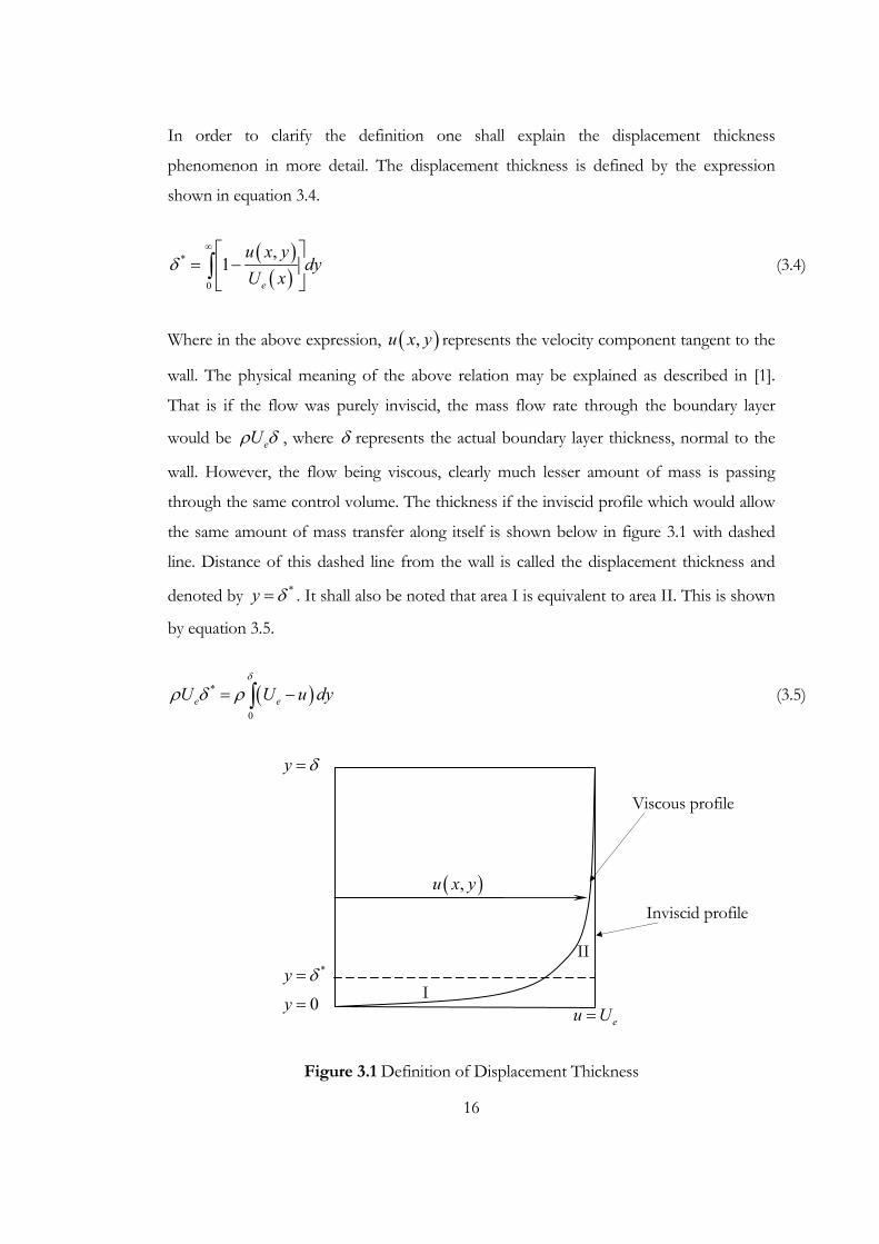
In order to clarify the definition one shall explain the displacement thickness

phenomenon in more detail. The displacement thickness is defined by the expression

shown in equation 3.4.

( )( )

*

0

,1

e

u x ydy

U xδ

∞ ⎡ ⎤= −⎢ ⎥

⎣ ⎦∫ (3.4)

Where in the above expression, ( ),u x y represents the velocity component tangent to the

wall. The physical meaning of the above relation may be explained as described in [1].

That is if the flow was purely inviscid, the mass flow rate through the boundary layer

would be eUρ δ , where δ represents the actual boundary layer thickness, normal to the

wall. However, the flow being viscous, clearly much lesser amount of mass is passing

through the same control volume. The thickness if the inviscid profile which would allow

the same amount of mass transfer along itself is shown below in figure 3.1 with dashed

line. Distance of this dashed line from the wall is called the displacement thickness and

denoted by *y δ= . It shall also be noted that area I is equivalent to area II. This is shown

by equation 3.5.

( )*

0e eU U u dy

δ

ρ δ ρ= −∫ (3.5)

Figure 3.1 Definition of Displacement Thickness

Inviscid profile( ),u x y

y δ=

0y =eu U=

Viscous profile

I

II*y δ=

17

Changing the upper limit of the integral in equation 3.5 from δ to infinity has no

significant effect since at the edge of the boundary layer, it can be told that:

( ), ( )eu x y U x≅ (3.6)

The reasoning of the use of strong interaction approach can be explained as it simplifies

the process bringing a relation between displacement thickness and edge velocity

distribution as shown above.

3.2 Solution of the Standard Problem

Since the boundary layer equations are parabolic, marching technique is applicable starting

from a known solution at say 0x x= . As one proceeds in downstream direction, since the

thickness of the boundary layer increases, one has to maintain sufficiently high resolution,

in order to keep increments in stream-wise direction small, in order to maintain

computational accuracy. In order to solve equation 2.19, one may solve it as it is, or

introduce a more convenient form by using a similarity transformation which eliminates

the problems related to the boundary layer growth phenomenon and therefore the

restrictions in stream-wise grid spacing.

A widely used similarity transformation is the Falkner-Skan transformation, which is a

consequence of group theoretic method described by Hansen in reference [16]. In

Falkner-Skan transformation, x values remain unchanged, even in some cases they are

denoted by the Greek letter ξ . The similarity variables used in Falkner-Skan

transformation is the dimensionless distance in normal direction that is y-direction, η

which is given below in equation 3.7.

eU yx

ην

= (3.7)

And the corresponding dimensionless stream function ( , )f x η is given in equation 3.8

below.

18

( ) ( ), ,ex y U x f xψ ν η= (3.8)

In equation 3.8, ψ is the dimensional stream function, from which the velocity

components may be written as shown below in equation 3.9.

uyψ∂

=∂

(3.9a)

vxψ∂

= −∂

(3.9b)

Using the prescribed similarity transformation, differentiation with respect to x and y

terms become:

y xx x x ηη⎛ ⎞∂ ∂ ∂ ∂⎛ ⎞ ⎛ ⎞= +⎜ ⎟ ⎜ ⎟⎜ ⎟∂ ∂ ∂ ∂⎝ ⎠ ⎝ ⎠⎝ ⎠

(3.10a)

xxy yη⎛ ⎞ ⎛ ⎞∂ ∂ ∂

=⎜ ⎟ ⎜ ⎟∂ ∂ ∂⎝ ⎠⎝ ⎠ (3.10b)

Falkner-Skan transformation enables one to generate initial condition at and near the

stagnation point, and results in the boundary layer equations to become ordinary

differential equations rather than partial ones for similar flows. However, its use is not

limited to similar flows since even if it does not eliminate, it significantly decreases the

dependence in stream-wise position. The latter is valid for the case investigated as the

presence of x as a variable can be recognized from equation 3.10.

Defining ξ as the dimensionless surface distance as /x Lξ = , L being the characteristic

length of the flow, and applying the above transformation to equation 2.19 yields equation

3.11 which is given below.

( ) ( )21 12m f fbf ff m f f fξ

ξ ξ′⎛ ⎞+ ∂ ∂′ ⎡ ⎤′′ ′′ ′ ′ ′′+ + − = −⎜ ⎟⎣ ⎦ ∂ ∂⎝ ⎠

(3.11)

And the corresponding boundary conditions are given below in equation 3.12.

19

0f ′ = , 0f = at 0η = (3.12a)

1f ′ = at eη η= (3.12b)

In equation 3.12, eη is the dimensionless coordinate corresponding to the edge of the

boundary layer as stated in [7]. The definition is given below in equation 3.13.

L ee

R ULδη

ξ= (3.13)

In equation 3.11, primes denote differentiation with respect to the transformation variable

η . Also one shall note that m is the dimensionless pressure gradient defined below in

equation 3.14 and tν+ being the fraction of eddy viscosity to kinematic viscosity of the

fluid. Notice that, definition for the term b is altered to make it also dimensionless as

defined by equation 3.16.

e

e

dUmU dξ

ξ= (3.14)

mt

ενν

+ = (3.15)

1 tb ν += + (3.16)

Equation 3.16 is valid both for laminar and turbulent flows, and its value becomes unity in

case of laminar flows.

In order to solve equation 3.11 together with its boundary conditions, Keller’s box

scheme is employed as explained above. This scheme is essentially a two point finite-

difference scheme, in which the equation itself and the boundary conditions are expressed

as a system of three equations of the first-order. In order to achieve this goal, new

variables are introduced to express derivatives of f . In Keller’s box scheme, the variables

are evaluated at the vertices, where the equations are written for the center of the box.

20

Figure 3.2 Rectangular grid used for centered difference approximation.

The nodes of the above rectangular grid are chosen as:

1n n nkξ ξ −= + 1,2,3, ,n N= (3.17a)

1j j jhη η −= + 1,2,3, ,j J= (3.17b)

As the resultant system of equations is non-linear, Newton’s method, which is introduced

in subsection 3.2.2 is used for linearization, and then solved by the block elimination

method described in subsection 3.2.3.

3.2.1 Numerical Scheme

As described above in section 3.2 new variables are introduced to represent derivatives of

f , enabling one to write equation 3.11 and its associated boundary conditions 3.12 as a

system of first order equations. Note that the newly introduced variables are not velocity

components but the derivatives of the non-dimensional stream function f with respect

to similarity variable η . Defining ( , )u x η and ( , )v x η such that:

f u′ = (3.18a)

f u v′′ ′= = (3.18b)

η

jη

1jη −

ξ1nξ − nξ

jη

1jη −

1nξ − nξ1/ 2nξ −

1/ 2jη − jh

nk

21

Using these new variables, eqs.3.11 and 3.12 are rewritten as eqs.3.19 and 3.20.

( ) 21 12m u fbv fv m u u vξ

ξ ξ⎛ ⎞+ ∂ ∂′ ⎡ ⎤+ + − = −⎜ ⎟⎣ ⎦ ∂ ∂⎝ ⎠

(3.19)

0u = , 0f = at 0η = (3.20a)

1u = at eη η= (3.20b)

Writing equation 3.18 in discrete form using Keller’s box method yields:

1 11/ 22

n n n nj j j j n

jj

f f u uu

h− −

−

− += ≡ (3.21a)

1 11/ 22

n n n nj j j j n

jj

u u v vv

h− −

−

− += ≡ (3.21b)

With L denoting the LHS, and R denoting the RHS, equation 3.19 can be approximated

at the center of the rectangle by first centering in ξ direction as shown below in equation

3.22.

( )1 1

1 1/ 2 1/ 2 1/ 212

n n n nn n n n n

n n

u u f fL L u vk k

ξ− −

− − − −⎡ ⎤⎛ ⎞ ⎛ ⎞− −+ = −⎢ ⎥⎜ ⎟ ⎜ ⎟

⎝ ⎠ ⎝ ⎠⎣ ⎦ (3.22)

Where:

( ) 21 12

nn mL bv fv m u+⎡ ⎤′ ⎡ ⎤= + + −⎣ ⎦⎢ ⎥⎣ ⎦

(3.23a)

( )1

1 21 12

nn mL bv fv m u

−− +⎡ ⎤′ ⎡ ⎤= + + −⎣ ⎦⎢ ⎥⎣ ⎦

(3.23b)

Defining nα as in equation 3.24 one can rewrite equation 3.22 as shown in equation 3.25.

22

1/ 2nn

nkξα

−

= (3.24)

( ) ( ) 12 1 1 1 2 1 1n nn n n n n n n n n n n nL u v f v f v f L u f vα α−− − − − −⎡ ⎤ ⎡ ⎤− − − + = − + − +⎢ ⎥ ⎢ ⎥⎣ ⎦ ⎣ ⎦

(3.25)

Since the values having the superscript ( )1n− are known from the previous station, and

one is trying to obtain the values of current station, one may rearrange terms in equation

3.22 and obtain:

( ) ( ) ( ) ( )2 1 1 11 2

nnn n n n n n nbv fv u f v v f Rα α α − − −⎡ ⎤′ ⎡ ⎤+ − + − =⎣ ⎦⎢ ⎥⎣ ⎦

(3.26)

In the above equation the newly introduced variables are:

11

2

nnmα α+

= + (3.27a)

2n nmα α= + (3.27b)

( ) 11 1 1 1 2 nn n n n n nR L v f u mα−− − − −⎡ ⎤= − + − −⎢ ⎥⎣ ⎦

(3.27c)

As now the equation 3.19 is centered in ξ direction, one may proceed to center it in η

direction, that is to write it at 1/ 2jη − .

( ) ( ) ( ) ( )1 1 2 1 1 11 2 1/ 2 1/ 2 1/ 2 1/ 2 1/ 21/ 2 1/ 2

n nnnj j j j n n n n n n

j j j j jj jj

b v b vfv u f v f v R

hα α α− − − − −

− − − − −− −

−⎡ ⎤+ − + − =⎣ ⎦ (3.28)

Where:

( ) 11 1 1 1 21/ 2 1/ 2 1/ 2 1/ 2 1/ 2

nn n n n n nj j j j jR L v f u mα

−− − − −− − − − −

⎡ ⎤= − + − −⎢ ⎥⎣ ⎦ (3.29a)

23

( ) ( ) ( ) ( )1

1 11 21/ 2 1/ 2 1/ 2

1 12

n

j j j jnj j j

j

b v b v mL fv m uh

−

− −−− − −

⎧ ⎫− +⎪ ⎪⎡ ⎤= + + −⎨ ⎬⎢ ⎥⎣ ⎦⎪ ⎪⎩ ⎭ (3.29b)

Note that equations 3.21 and 3.28 are imposed for 1,2,3, , 1j J= − at any given η . For

0j = and j J= , the boundary conditions given in equation 3.20 are used. The

transformed boundary layer thickness, eη , has to be sufficiently large, so that 1eU →

asymptotically. This is usually satisfied when ( ) 310ev η −< .

Also the boundary conditions given in equation 3.20 can be written in discrete form as

shown in equation 3.30.

0 0nf = 0 0nu = at 0j = (3.30a)

1nJu = at j J= (3.30b)

3.2.2 Newton’s Method

As the above derived discretized system of equations is non-linear, one has to linearize

them in order to solve them in matrix form. In order to accomplish this objective, small

perturbation quantities for all of the variables are introduced, and an iterative scheme

called Newton’s method is employed.

As an initial guess, values of the variables at the previous station are used. Note that in the

below expression, k stands for the order of iteration, δ represents perturbation

quantities.

1k k kj j jf f fδ+ = + (3.31a)

1k k kj j ju u uδ+ = + (3.31b)

1k k kj j jv v vδ+ = + (3.31c)

24

After substituting the above quantities into eqns.3.21 and 3.28, one obtains the following

set of equations after neglecting higher order terms.

( ) ( ) ( ) ( )1 1 1 1 12 2j jn n n n n n n n

j j j j j j j j j

h hf f u u u u f f rδ δ δ δ− − − −− − + = − − − = (3.32)

( ) ( ) ( ) ( )1 1 1 1 3 12 2j jn n n n n n n n

j j j j j j j j j

h hu u v v v v u u rδ δ δ δ− − − − −

− − + = − − − = (3.33)

( ) ( ) ( ) ( ) ( ) ( ) ( )1 2 1 3 4 1 5 6 1 2n n n n n nj j j j j jj j j j j j j

s v s v s f s f s u s u rδ δ δ δ δ δ− − −+ + + + + = (3.34)

Where r terms are:

( ) ( )1 1 1/ 2j j j jjr f f h u− −= − + (3.35a)

( ) ( )3 1 1/ 2j j j jjr u u h v− −= − + (3.35b)

( ) ( ) ( ) ( )1 11 2 1 12 1/ 2 1 2 1/ 2 1/ 2 1/ 2 1/ 21/ 2 1/ 2

nnnj j j jn n n n n n n

j j j j jj jj

b v b vr R fv u v f f v

hα α α α− −− − −

− − − − −− −

−= − − + − + (3.35c)

The coefficients of the perturbation quantities appearing above in equation 3.34 are as

given in equation 3.36.

( ) 1 111 1/ 22 2

nn n n

j j j jjs h b f fα α− −

−= + − (3.36a)

( ) 1 112 1 1 1 1/ 22 2

nn n n

j j j jjs h b f fα α− −

− − − −= − + − (3.36b)

( ) 113 1/ 22 2

nn nj jj

s v vα α −−= + (3.36c)

( ) 114 1 1/ 22 2

nn nj jj

s v vα α −− −= + (3.36d)

25

( )5 2njj

s uα= − (3.36e)

( )6 2 1njj

s uα −= − (3.36f)

The boundary conditions also change as the perturbation equations applied, and become

as shown below:

0 0n n

wf f fδ+ = 0 0nfδ = (3.37a)

0 0 0n nu uδ+ = 0 0nuδ = (3.37b)

1n nJ Ju uδ+ = 0n

Juδ = (3.37c)

Equations 3.32-3.34 are written for each j-station starting from the wall, extending to the

edge of the boundary layer and will be represented in matrix notation as in equation 3.38.

[ ] { } { }A rδ⋅ = (3.38)

Defining terms in the above equation:

A is the tri-diagonal coefficient matrix defined as:

[ ]

0

1 1 1

2 2 2

1 1 1

o

j j j

J J J

J J

A CB A C

B A C

AB A C

B A CB A

− − −

⎡ ⎤⎢ ⎥⎢ ⎥⎢ ⎥⎢ ⎥⎢ ⎥= ⎢ ⎥⎢ ⎥⎢ ⎥⎢ ⎥⎢ ⎥⎢ ⎥⎣ ⎦

(3.39)

And δ is the vector of unknowns.

26

[ ]

0

1

j

J

δδ

δδ

δ

⎧ ⎫⎪ ⎪⎪ ⎪⎪ ⎪⎪ ⎪= ⎨ ⎬⎪ ⎪⎪ ⎪⎪ ⎪⎪ ⎪⎩ ⎭

[ ]

0

1

j

J

rr

rr

r

⎧ ⎫⎪ ⎪⎪ ⎪⎪ ⎪⎪ ⎪= ⎨ ⎬⎪ ⎪⎪ ⎪⎪ ⎪⎪ ⎪⎩ ⎭

(3.40a,b)

The elements in equation 3.40 are vectors defined as follows:

j

j u

j

fuv

δδ δ

δ

⎧ ⎫⎪ ⎪= ⎨ ⎬⎪ ⎪⎩ ⎭

1

2

3

( )( )( )

j

j j

j

rr r

r

⎧ ⎫⎪ ⎪= ⎨ ⎬⎪ ⎪⎩ ⎭

0 j J≤ ≤ (3.41a,b)

In addition, elements of matrix A shown in equation 3.39 are sub-matrices for which

definitions are given below in equation 3.42.

0

1

1 0 00 1 00 1 / 2

Ah

⎡ ⎤⎢ ⎥= ⎢ ⎥⎢ ⎥− −⎣ ⎦

(3.42a)

( ) ( ) ( )3 5 1

1

1 / 2 0

0 1 / 2

j

j j j j

j

hA s s s

h +

⎡ ⎤− −⎢ ⎥

= ⎢ ⎥⎢ ⎥

− −⎢ ⎥⎣ ⎦

1 1j J≤ ≤ − (3.42b)

( ) ( ) ( )3 5 1

1 / 2 0

0 1 0

J

J J J J

hA s s s

−⎡ ⎤⎢ ⎥= ⎢ ⎥⎢ ⎥⎣ ⎦

(3.42c)

( ) ( ) ( )4 6 2

1 / 2 0

0 0 0

j

j j j j

hB s s s

⎡ ⎤− −⎢ ⎥

= ⎢ ⎥⎢ ⎥⎣ ⎦

1 j J≤ ≤ (3.42d)

27

1

0 0 00 0 00 1 / 2

j

j

Ch +

⎡ ⎤⎢ ⎥= ⎢ ⎥⎢ ⎥−⎣ ⎦

0 1j J≤ ≤ − (3.42e)

3.3 Inverse Problem

Since the standard problem can not handle separated regions as in attached regions, the

edge velocity can not be calculated, one has to switch from the standard problem to the

inverse problem. In this study, this switching is automatically done by the computer code

utilized after a few stations in x-direction. For further information see reference [1].

The procedure described above in section 3.2 will be modified to handle the inverse

problem. When the displacement thickness is specified, one can establish a relationship

between the displacement thickness and the edge velocity. In order to establish such a

relationship the solution procedure is modified as described in subsection 3.3.1.

3.3.1 Solution Procedure for Specified Displacement Thickness

Consider an external flow case where the displacement thickness distribution is given as

( )* xδ . The boundary conditions for such a problem would be:

0y = ; 0u = , 0v = (3.43a)

y δ= ; eu u= , ( )* xδ as specified. (3.43b)

One shall follow the same procedure described in section 3.2 and start with a

transformation. The difference is that, in this case, since the edge velocity distribution eU ,

is unknown and therefore can not be used in the definition of the transformation variable.

For this reason, the edge velocity distribution is replaced by the free-stream velocity, U∞ ,

so that the new transformation becomes:

UY yxν∞= (3.44a)

28

( , )U xF Yψ ν ξ∞= (3.44b)

Using these new transformation variables, the boundary layer equations and the

corresponding boundary conditions are rewritten as below.

( ) 12

eedUF FbF FF F F Ud

ξ ξξ ξ ξ′⎛ ⎞∂ ∂′′′ ′′ ′ ′′+ = − −⎜ ⎟∂ ∂⎝ ⎠

(3.45)

0Y = 0F ′ = , 0F = (3.46a)

eY Y= ( )e eF U ξ′ = , ( ) ( )*

Lee

e

RF Y eF L

δ ξξ

ξ= − ≡′

(3.46b)

Where in the above formulations, L is the characteristic length and primes denote

differentiation with respect to transformation variable, Y. Other newly introduced

variables are given in equation 3.47.

xL

ξ = , (3.47a)

LU LRν∞= , (3.47b)

eeUUU∞

= (3.47c)

For the edge boundary condition, we may use the definition of displacement thickness as

shown in equation 3.48 if its value is known prior to these calculations.

( )* ee

eL

L FYFR

ξδ ξ

⎛ ⎞= −⎜ ⎟′⎝ ⎠

(3.48)

Since in the inverse problem value of eU is unknown, it has to be integrated into the

solution. In order to do it, a new variable is introduced.

29

( )ew U ξ= (3.49)

And since the edge velocity is a function of ξ only: ( )w ξ , one may write the following

equation.

0w′ = (3.50)

The next step is to reduce the order of the partial differential equation (PDE) of equation

3.45 as in equation 3.51.

F U′ = (3.51a)

F U V′′ ′= = (3.51b)

( ) 12

U F dwbV FV U V wd

ξ ξξ ξ ξ

⎛ ⎞∂ ∂′ + = − −⎜ ⎟∂ ∂⎝ ⎠ (3.51c)

0w′ = (3.51d)

According to the new PDE, the new boundary conditions are:

0Y = 0F U= = (3.52a)

eY Y= U w= , ( )F e wξ= (3.52b)

In order to solve these equations in a rectangular grid, one has to discretize them by

employing finite difference approximations.

11/ 2

j jj

j

F FU

h−

−

−= (3.53a)

11/ 2

j jj

j

U UV

h−

−

−= (3.53b)

30

1 0n nj j

j

w wh

−−= (3.53c)

( ) ( ) ( )1 1 1 11 1 1/ 2 1/ 2 1/ 2 1/ 2 1/ 21/ 2

12

nn n n n n n n n n n nj j j j j j j j j jjh b V b V FV V F F V Rα α− − − −

− − − − − − −−

⎛ ⎞− + + + − =⎜ ⎟⎝ ⎠

(3.53d)

Where

( ) ( ) 11 21/ 2 1/ 2 1/ 2 1/ 2

nnn n nj j j jR L FV uα

−−− − − −

⎡ ⎤= − + −⎢ ⎥⎣ ⎦ (3.54a)

( ) ( ) ( )1

1 11 21/ 2 1/ 2 1/ 2

12

n

j j j jn nj j j

j

b V b VL FV w

hα

−

− −−− − −

⎧ ⎫−⎪ ⎪= + −⎨ ⎬⎪ ⎪⎩ ⎭

(3.54b)

Note that in equation 3.54b, 1n − in the RHS means, value at station n-1.

If one compares these equations with those of equation 3.26, it is clear that of one sets

0m = in eqs.3.27, the results will be:

112

nα α= + (3.55a)

2nα α= (3.55b)

The final step is to linearize these equations in the same manner as in subsection 3.2.2.

Note that there is one new variable w , and hence a corresponding perturbation has to be

introduced for w .

( ) ( ) ( ) ( )1 1 1 1 12 2j jn n n n n n n n

j j j j j j j j j

h hF F U U U U F F rδ δ δ δ− − − −− − + = − − − = (3.56a)

( ) ( ) ( ) ( )1 1 1 1 3 12 2j jn n n n n n n n

j j j j j j j j j

h hU U V V V V U U rδ δ δ δ− − − − −

− − + = − − − = (3.56b)

( )1 1j j j jw w w wδ δ − −− = − (3.56c)

31

Recall that r terms are:

( ) ( )1 1 1/ 2j j j jjr F F h U− −= − + (3.35a)

( ) ( )3 1 1/ 2j j j jjr U U h V− −= − + (3.35b)

( ) ( ) ( ) ( )1 11 2 1 12 1/ 2 1 2 1/ 2 1/ 2 1/ 2 1/ 21/ 2 1/ 2

nnnj j j jn n n n n n n

j j j j jj jj

b V b Vr R FV U V F F V

hα α α α− −− − −

− − − − −− −

−= − − + − + (3.35c)

Equation 3.57 is written very much like equation 3.34 except for two additional terms

coming from the introduction of our new variable.

( ) ( ) ( ) ( ) ( )( ) ( ) ( ) ( )1 2 1 3 4 1 5

6 1 7 8 1 2

j j j j jj j j j j

j j jj j j j

s V s V s F s F s U

s U s w s w r

δ δ δ δ δ

δ δ δ

− −

− −

+ + + +

+ + + = (3.57)

And the definitions of the s terms are given by equation 3.36, except for ( )7 js and

( )8 js , which are given by equation 3.58.

( ) 1 111 1/ 22 2

nn n n

j j j jjs h b f fα α− −

−= + − (3.36a)

( ) 1 112 1 1 1 1/ 22 2

nn n n

j j j jjs h b f fα α− −

− − − −= − + − (3.36b)

( ) 113 1/ 22 2

nn nj jj

s v vα α −−= + (3.36c)

( ) 114 1 1/ 22 2

nn nj jj

s v vα α −− −= + (3.36d)

( )5 2njj

s uα= − (3.36e)

( )6 2 1njj

s uα −= − (3.36f)

32

( )7n

jjs wα= (3.58a)

( )8 1n

jjs wα −= (3.58b)

The new, linearized boundary conditions are as of equation 3.59.

0 0Fδ = (3.59a)

0 0Uδ = (3.59b)

J J J JU w w Uδ δ− = − (3.59c)

( )n nJ J J JF e w e w Fδ δ− = − (3.59d)

The above discrete equation set is written in matrix form just as in section 3.2. except that

sub-matrices in [ ]A will be 4×4 rather that 3×3.

[ ] { } { }A rδ⋅ = (3.38)

[ ]A is a tri-diagonal matrix with the same form of equation 3.39, except that sub-matrices

in [ ]A will be 4×4 rather that 3×3. Fist two rows of the element matrices 0A and 0C ,

and the last two rows of the element matrices JB and JA constitute the boundary

conditions. Likewise, the vectors { }δ and { }r remain the same with element vectors of

them jδ and jr are now 4×1 vectors.

The solution method is again the block elimination method, which is explained in

appendix A.

3.3.2 Interaction Procedure

In order to solve separated flows with the inverse method described above, one has to

specify either the displacement thickness or the wall shear as noted in [9]. In order to

33

solve for external flows as intended in this study, a potential flow solver is required to

calculate the edge velocity distribution, which enables one to solve the boundary layer

equations in inverse mode. The interaction is accomplished via the blowing velocity

distribution as described in equation 1.1. The blowing velocity itself, serves as a boundary

condition for the next step of the potential flow calculations.

In order to solve the boundary layer equations, the blowing velocity concept in Veldman’s

suggestion is used as discussed in section 3.1. Rewriting equation 3.2 using definition

given in equation 3.3, one obtains equation 3.60.

0( ) ( ) ( )e e eU x U x U xδ= + (3.2)

( ) ( )*1( )

b

a

x

e ex

d dU x Ud x

ξδ δπ ξ ξ

=−∫ (3.3)

( ) ( )0 *1( ) ( )e i e i e

i

d dU x U x Ud x

ξδπ ξ ξ

= +−∫ (3.60)

The Hilbert integral in the above equation can be approximated as described in appendix

B, to yield:

( ) ( ) ( ) ( )0 *

1

N

e i e i ij i jj

U x U x C x xδ=

= +∑ (3.61)

( ) ( ) ( ) ( )* 0 *e i ii i e i ij j i

j i

U x C x U x C x gδ δ≠

− = + =∑ (3.62)

Rewriting equation 3.48 as in equation 3.63 and substituting into equation 3.62, one may

get equation 3.64.

( )* e ei e e

e eL

L Fx y YU UR

ξψδ⎛ ⎞

= − = −⎜ ⎟⎝ ⎠

(3.63)

( ) ee i ii e i

e

U x C y gUψ⎡ ⎤

− − =⎢ ⎥⎣ ⎦

(3.64)

34

Since the above formulation is non-linear, one has to linearize it in eψ and eU to use as a

boundary condition.

[ ]e e ii iU U C p p gδ δ+ − + = (3.65)

Where the term p and pδ in the above equation is defined by equation 3.66

( )( )

e ie

e i

xp y

U xψ

= − (3.66a)

2e e

ee e

p UU Uδψ ψδ δ−

= + (3.67b)

Hence the linearized equation becomes equation 3.68.

21ii e ee ii e i e ii e

e e e

C C U g U C yU U U

ψ ψδψ δ⎛ ⎞ ⎛ ⎞ ⎛ ⎞

+ + = − + −⎜ ⎟ ⎜ ⎟ ⎜ ⎟⎝ ⎠ ⎝ ⎠ ⎝ ⎠

(3.68)

From the above equations, one can easily note that in order to calculate ig , ijC and

( )*jxδ have to be known. In order to calculate them, sweeps within the boundary layer

are performed. For j i> , the displacement thickness values are taken from the previous

sweep and in case j i< , values calculated in the current sweep are used. With this

additional information, one can now proceed to calculate the summation term in equation

3.62 in an iterative manner. Once it is converged, the calculations proceed to the next x

station where the whole process is repeated. For calculation of coefficients iiC , refer to

appendix B.

3.4 Solution Procedure for the Wake Region

As described thoroughly in [1], solution procedure for the wake region is much more

complex compared to solution on the body itself. In order to eliminate problems related

to transition from no-slip wall boundary condition to smooth flow in the wake region,

one has to prepare an extremely fine grid near the trailing edge of a lifting section in order

35

to impose this change gradually to the solution domain. One of the major difficulties in

wake calculation is that since at high angles-of-attack, the boundary layer coming from the

upper surface is turbulent, separated and thick compared to a thin, laminar or transitional

boundary layer coming from the lower surface, merging process of these boundary layers

is complicated, and may be considered like a mixing layer with considerable backflow.

In order to solve the boundary layer equations within the wake region, one has to recall

equation 2.19.

eedUu u uu v U b

x y dx y y⎛ ⎞∂ ∂ ∂ ∂

+ = + ⎜ ⎟∂ ∂ ∂ ∂⎝ ⎠ (2.19)

As in the case of wall boundary layers, the above equation is written as a system of first

order equations as shown in equation 3.51.

F U′ = (3.51a)

U V′ = (3.51b)

( ) 12

U F dwbV FV U V wd

ξ ξξ ξ ξ

⎛ ⎞∂ ∂′ + = − −⎜ ⎟∂ ∂⎝ ⎠ (3.51c)

0w′ = (3.51d)

However, the boundary conditions for the wake region are different, and are given as:

F w′ = at eY Y−= (3.69a)

0F = at 0Y = (3.69b)

F w′ = at eY Y= (3.69c)

( ) ( )ii e e e e iw C w Y Y F F g− −− − − − =⎡ ⎤⎣ ⎦ (3.69d)

36

Where

12

0ii iiC C

Uνξ⎛ ⎞

= ⎜ ⎟⎝ ⎠

(3.70)

Where eY and eY− are the values of the transformation variable at the upper and lower

edges of the boundary layer for the wake region respectively. Similarly, eF and eF− are the

values for the dimensionless stream function for the upper and lower edges. In order to

stabilize the solutions of the above system, its sensitivity to the boundary conditions

involving the dimensionless stream function is reduced by employing the so called Mechul

function prescribed in reference [3]. With the introduction of Mechul function, eF− is

denoted by s . And as s is a function of x only one may write,

0s′ = (3.71)

The boundary conditions for the system given in equation 3.69 can now be rewritten as:

F w′ = , es F−= at eY Y−= (3.72a)

0F = at 0Y = (3.72b)

( ) ( )ii e e e i

F w

w C w Y Y F s g−

′ = ⎫⎪⎬− − − − =⎡ ⎤ ⎪⎣ ⎦ ⎭

at eY Y= (3.72c)

The solution procedure is pretty much the same as of the above sections, expect that the

elements of matrix [ ]A , which are sub-matrices are now 5×5. Accordingly the vectors

{ }δ and { }r become 5×1 vectors, and solved using the block elimination method

described in appendix A.

37

C H A P T E R 4

TRANSITION METHOD IN 2D INCOMPRESSIBLE FLOWS

Early attempts to understand turbulence phenomenon focused on the original laminar

flow, and tried to explain the reasons of its end, which is the start of the turbulent flow.

Rayleigh introduced the inflectional instability and worked mainly on inviscid flows until

Taylor and Prandtl introduced the effects of viscosity. A complete boundary layer

instability theory was first introduced by Tollmien and Schlichting, who also calculate the

amplification rates for most of the unstable frequencies. After the experiments carried out

by Schubauer and Skramstad in 1947, which demonstrated the presence of two

dimensional sinusoidal instability waves within a boundary layer, their connection with

transition and quantitative description were given by the theory of Tollmien and

Schlichting. It was in 1956 that the en transition prediction method was introduced by

Smith, Gamberon and van Ingen, which is still in use today and is the basis of this study.

Pretch provided a large amount of numerical results by calculating the stability

characteristics of Falkner-Skan velocity profiles in 1942. Further reading is available in

reference [17].

The balance between stabilizing viscous forces and destabilizing shear forces are

represented by the critical Reynolds number. Perturbations that lead to instabilities arise

from small changes in the boundary conditions which may be due to free-stream

turbulence, surface roughness, noise, etc. which constitute the so called disturbance

environment. The problem about how these disturbances are entrained in the flow is

related to the subject of receptivity.

Receptivity may be defined as the mechanisms that cause the above described

disturbances to enter the flow which yield the creation of the initial amplitudes for the

waves generating instabilities. These disturbances are usually very small so that they can

not be measured using the modern instruments until the instabilities are developed. To

date, this mechanism still remains as not fully understood.

38

The initial growth of the two dimensional Tollmien-Schlichting waves can be described by

the linear stability theory which constitutes the basis of the famous Smith-van Ingen en

transition prediction method. After their growth, three dimensional waves and/or non-

linear interactions are observed, which means that normally the linear stability theory can

no longer be used. However, a bracketing assumption that extends the use of linear

stability theory until transition is employed. The transition data obtained from such an

approach has been shown to agree acceptably for most of the engineering problems of

interest.

Currently the most popular method for predicting transition which is accepted as an

engineering tool is the so called Smith-van Ingen en transition prediction method. As

briefly discussed in chapter 1, it is based on solution of two-dimensional linear stability

equations which are given by the fourth order ordinary differential equation (ODE) called

the Orr-Sommerfeld equation given in equation 1.2. Derivation of this equation is

explained in detail in Appendix C.

2 4 2( 2 ) [( )( ) ]iv iR u uφ α φ α φ α ω φ α φ α φ′′ ′′ ′′− + = − − − (1.2)

In the above equation, primes denote differentiation in the normal direction, u denotes

the velocity profile in the stream-wise direction. Finally ( ) ( )r iy iφ φ φ≡ + represents the

complex amplitude of the disturbance stream function ψ defined by the fluctuating

velocity components u and v defined as shown in equation 4.1. In the below equation,

hats stand for fluctuating quantities.

ˆu

yψ∂

=∂

ˆ

vxψ∂

= −∂

(4.1)

The parameter α is the wave-number of the disturbance which is related to the

wavelength λ via equation 4.2, where ω is the circular frequency, whose unit is either

radians per second or Hertz.

2πλα

= (4.2)

39

The case where the wave-number is complex ( )r iiα α α≡ + but the circular frequency is

real is called the spatial amplification theory in which the amplitude of the disturbance

varies with stream-wise position as ( )exp i xα− . On the other hand the case when the

circular frequency is complex ( )r iiω ω ω≡ + , but the wave-number is real is called the

temporal amplification theory in which the amplitude varies with time as ( )exp itω− .

These two may be related to each other using the Gaster’s transformation. These theories

are discussed in great detail in references [5, 11, 17 and 18]. Also some more information

is available in references [19, 20].

For the sake of convenience, quantities are transformed into their respective

dimensionless forms. In order to non-dimensionalize the Orr-Sommerfeld equation given

above, a dimensionless time variable is introduced as:

UtL

τ ∞= (4.3)

Where L is the reference length, defined as the characteristic length of the flow in the

above sections, namely chord for external flows. Dividing all the velocity terms by the

reference velocity, which is the free-stream velocity for external flows, and all lengths by

the reference length, the dimensionless Orr-Sommerfeld equation becomes:

( )( )2 4 22ivL L L L LiR u uφ α φ α φ α ω φ α φ α φ⎡ ⎤′′ ′′ ′′− + = − − −⎣ ⎦ (4.4)

Note that in the above equation primes denote differentiation with respect to

dimensionless distance in the normal direction as y∂∂

where y bar term is defined as

yyL

= . With the proper choice of L , the non-dimensional distance in the normal

direction becomes the same as the one used in the boundary layer calculations. Also

( )yφ is the complex amplitude of the disturbance stream function ( ), ,x yψ τ′ defined

as shown in equation 4.5.

40

( ) ( ) ( ), , exp Lx y y i xψ τ φ α ωτ′ = −⎡ ⎤⎣ ⎦ (4.5)

Where

L Lα α= (4.6a)

uuU∞

= (4.6b)

UL

ω ω∞= (4.6c)

U LRν∞= (4.6d)

In order to solve for equation 4.4, the boundary conditions are given in equation 4.7.

Wall B.C.: 0y = 0y = , 0φ = , 0φ′ = (4.7a)

Infinity B.C.: y→∞ ˆ ˆ 0u v= = (4.7b)

It is convenient to write the infinity boundary condition by taking into account that

perturbation velocities will decay as the edge of the boundary layer is approached. In this

case, the infinity boundary condition may be satisfied at the edge of the boundary layer by

equation 4.8.

( ) ( )( )( )( )

21 1 2 1

2 22 1

0

0

D D

D D

ε φ ε ε ε φ

ε ε φ

⎫− + + + = ⎪⎬

+ − = ⎪⎭ at y

Lδ

= (4.8)

Where

dDdy

= (4.9a)

21 Lε α= (4.9b)

41

( )2 22 1 LiR uε ε α ω= + − (4.9c)

The onset of transition is obtained by solving the dimensionless Orr-Sommerfeld

equation with give boundary conditions and following the en procedure. The solution

procedure may either be based on the spatial amplification theory or the temporal

amplification theory.

In this study, the former one is preferred since the amplification of a disturbance can be

measured in a steady mean flow. Since in the spatial amplification theory, the amplitude at

a fixed point is independent of time, calculations of group velocities are not required. Also

the spatial amplification theory gives the change in amplification values in a more direct

manner than does the temporal theory as noted in [11].

4.1 Smith-van Ingen en Procedure

The en procedure requires the calculation of the amplification factors denoted by ( )iα−

as a function of either the stream-wise position or Reynolds number based on the stream-

wise distance for a range of dimensional frequencies defined by equation 4.10.

* UL

ω ω ∞= (4.10)

The laminar boundary layer equations for a given external velocity distribution denoted by

( )eU x and the free-stream Reynolds number denoted by R are solved to obtain stream-

wise velocity distribution u and its second derivative u′′ . Note that the amplification rate

term ( )iα− , represents damping if it is negative, a neutrally stable condition of it is zero,

and amplification when it is positive.

At a point where the instabilities begin say at 1x x= , shown in figure 4.1 by point 1,

where the amplification rate term transits from negative to positive, the eigenvalues rα

and ω are computed provided that the local velocity distribution, its second derivative

and the local Reynolds number are known. The dimensional frequency computed from

equation 4.10 is kept constant along line 1 which is determined by this frequency itself.

42

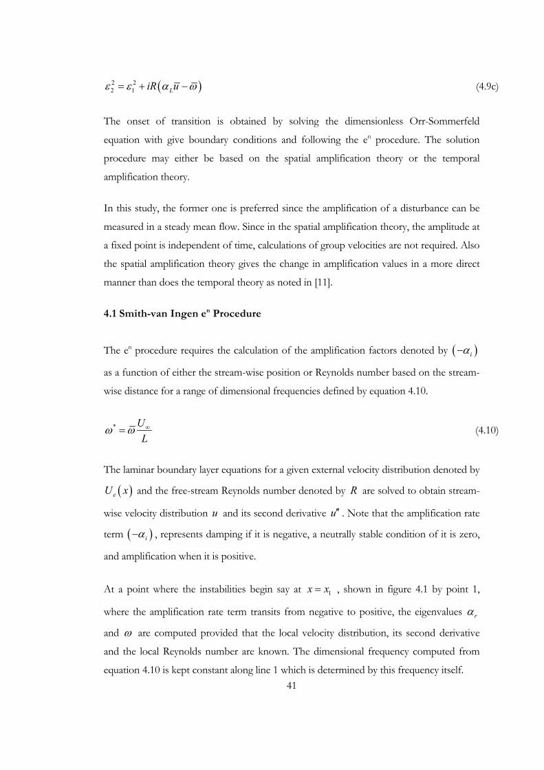
Figure 4.1 Schematic of transition calculation using en method

At the next location say 2x , two separate calculations are performed for the boundary

parameters which are newly computed. In one set of calculations the new eigenvalues are

computed on the neutral curve as shown by point 2 in the figure using the same

procedure explained for the prior station, so that a new dimensional frequency is obtained

which defines line 2. In the second set of calculations, point 1a, the dimensionless

frequency ω together with L and U∞ being known, is determined from the dimensional

frequency of line 1. With ω and the local Reynolds number of point 2 known, α is

obtained using the eigenvalue procedure.

The above explained procedure for point 1a is then repeated for points 2b and 1b

respectively and a dimensional frequency is computed for line 3. For example, at point 1b,

the values rα and iα are computed with the known dimensional frequency of line 1 and

the specified local Reynolds number at point 3. At point 2b, they are computed with the

known dimensional frequency of line 2 and specified Reynolds number of point 3.

This procedure is repeated for several number of lines (i.e. frequencies) specified by the

user and the variation of the integrated amplification rate defined by n is computed along

each line with 0x corresponding to the first value of x on the neutral stability curve.

line 1line 2

line 3

12

3

1a1b

2b

rα

xR

43

0

iRn dξ

ξ

α ξξ

⎛ ⎞= − ⎜ ⎟

⎝ ⎠∫ (4.11)

R E Y N O LD S

N

0 5 00 1 0 0 0 1 5 0 0 2 0 00 0 1 2 3 4 5 6 7 8 9

10 11 12 13 14

F R Q N UM= 2 ,PHYS. FRQ= 1536.13F R Q N UM= 3 ,PHYS. FRQ= 1184.51F R Q N UM= 4 ,PHYS. FRQ= 971.845F R Q N UM= 5 ,PHYS. FRQ= 828.402F R Q N UM= 6 ,PHYS. FRQ= 724.654F R Q N UM= 7 ,PHYS. FRQ= 645.873F R Q N UM= 8 ,PHYS. FRQ= 583.857F R Q N UM= 9 ,PHYS. FRQ= 533.673

Figure 4.2 Change in integrated amplification factor with respect to distance for Blasius

Flow

This procedure leads to curves of constant frequency, with each curve defining the

amplification rate as a function of the Reynolds number as shown in figure 4.2 and their

envelope corresponds to maximum amplification factors from which transition is

computed with a value of n which is commonly assumed between 8 and 9. Note that in

the above figure, the y-axis corresponds to amplification factor, where the x-axis

corresponds to the Reynolds number. As the figure shows Blasius flow, the Reynolds

number is defined as square root of local Reynolds number based on the stream-wise

distance due to the definition of Blasius length scale.

4.2 Numerical Scheme

Since the solution of the Orr-Sommerfeld equation is required in order to predict

transition, one has to apply a numerical scheme. The problem that requires attention is

44

that, since both the equation itself and all the boundary conditions are homogeneous; one

faces the problem of obtaining trivial solutions. It is only possible to end up with a non-

trivial solution, for some combinations of the Reynolds number, circular frequency and

the wave-number. Hence the problem becomes an eigenvalue problem in which values of

R , α and ω are the eigenvalues and the corresponding amplitude functions are

eigenfunctions. Note that subscript l in α , and bar on top of ω are dropped for the

sake of simplicity. Summarizing, there exists non-trivial solutions of the famous Orr-

Sommerfeld equation. In order to find such a solution, one has to define a relation such as

that of equation 4.12

( ), , 0F Rα ω = (4.12)

In this study, a finite difference method is employed which is again based on Keller’s box

scheme. Numerical formulation can be found below recalling again that subscript l in α ,

and bar on top of ω are dropped for the sake of simplicity.

21ε α= (4.9b)

( )2 22 1 iR uε ε α ω= + − (4.9c)

3 iR uε α ′′= (4.13)

With the introduction of 3ε the Orr-Sommerfeld equation can be written in a compact

form as below:

( )2 2 21 2 1 3 0ivφ ε φ ε φ ε φ ε φ′′ ′′− − − + = (4.14)

In order to write the above equation as an equivalent system of equations of the first

order, new parameters are defined. It is important to distinguish the newly introduced f

from the prior one used for the dimensionless stream-function.

fφ′ = (4.15a)

45

21f s ε φ′ = + (4.15b)

s g′ = (4.15c)

Hence the above equation 4.14 and its boundary conditions reduce to:

22 3g sε ε φ′ = − (4.16)

0y = ; { 0φ = , 0f = (4.17a)

yLδ

= ; ( ) ( )1 2 1 1 2

2

00

s fg s

ε ε ε ε ε φε

⎧ + + + + =⎪⎨

+ =⎪⎩ (4.17b)

In order to approximate the quantities ( ), , ,f s g φ , a mesh grid same as that of the

boundary layer solution is applied in the y-direction, where the edge of the boundary layer

is represented by Jy . As explained in the sections above, equation 4.15 is approximated

using a finite-difference method to yield:

( ) ( ) ( )1 3 1 1 0

jj j jj jc f f rφφ φ

− −− − + = = (4.18a)

( ) ( ) ( ) ( ) ( )1 3 1 1 1 3 10j j j j j jj j j

f f c s s c rφ φ− − − −− + + + + + = = (4.18b)

( ) ( ) ( )1 3 1 2 0j j j jj js s c g g r− −− − + = = (4.18c)

( ) ( ) ( ) ( ) ( )1 4 1 2 1 4 1 0j j j j j jj j jg g c s s c rφ φ− − − −

− + + + + + = = (4.18d)

With

( ) ( )21 1 3j jc cε= , ( ) ( ) ( )2 3 31/ 2j j j

c cε−

= − (4.19a, b)

( ) 1 13 2 2

j j jj

h y yc − −−

= = , ( ) ( ) ( )24 2 31/ 2j jjc cε

−= − (4.19c, d)

46

It is important to emphasize that, equations 4.18 are written in such a sequence that the

solution matrix [ ]A is non-singular, which means it has a non-zero determinant. In

addition, note that equations 4.18 are written for all values of j as: 1,2, , 1j J= −

where to values at 0j = and j J= are obtained from the boundary conditions which are

given below.

( )0 1 00rφ = = , ( )0 2 0

0f r= = (4.20a, b)

( ) ( ) ( )3 1 3 0J J JJ J Jf c s c rφ+ + = = (4.20c)

( ) ( )4 4J JJ Jg c s r+ = (4.20d)

Where

( )1 1Jc ε= , ( )3

1 2

1J

cε ε

=+

, ( )4 2Jc ε= (4.21)

Extensive care must be given for the solutions of these equations, since the Orr-

Sommerfeld equation itself and its boundary conditions are homogeneous, therefore

trivial solutions such as 0j j j jf s gφ= = = = are valid for all j for all values of α , ω

and R . In order to obtain a non-trivial solution, the eigenvalues and eigenfunctions have

to be calculated using an iteration procedure to find the values of parameters α , ω and

R to ensure that such a solution exists. Also one has to supply an external non-

homogeneous boundary condition to be satisfied. A clever idea offered by Cebeci et al. is

to change the boundary condition ( ) ( )00 0 0fφ′ = ≡ = with ( ) ( )00 1 1sφ′′ = ≡ = , so that

the difference equations may have a non-trivial solution since ( )0 0φ′′ ≠ . If one

determines the values of parameters using this suggestion, the original boundary condition

is satisfied and a non-trivial solution is obtained. This is achieved by an iterative scheme,

again based on Newton’s method as described in detail in sub-section 3.2.2 using equation

4.18 and wall boundary conditions given below:

( )0 1 00rφ = = , ( )0 2 0

1s r= = (4.22)

47

Also the edge boundary conditions given in equation 4.20 are written in matrix form as in

equation 3.38.

[ ] { } { }A rδ⋅ = (3.38)

However, in this case the vectors { }δ and { }r are different and given in equation 4.23.

j

jj

j

j

sfg

φ

δ

⎧ ⎫⎪ ⎪⎪ ⎪= ⎨ ⎬⎪ ⎪⎪ ⎪⎩ ⎭

( )( )( )( )

1

2

3

4

j

jj

j

j

r

rr

r

r

⎧ ⎫⎪ ⎪⎪ ⎪⎪ ⎪= ⎨ ⎬⎪ ⎪⎪ ⎪⎪ ⎪⎩ ⎭

(4.23a, b)

The sub-matrices jA , jB and jC , which are coefficients of matrix [ ]A (previously 3×3

but now 4×4 matrices) are given below in equation 4.24.

( ) ( )( ) ( )

01 31 1

2 41 1

1 0 0 00 1 0 0

1 00 1

Ac cc c

⎡ ⎤⎢ ⎥⎢ ⎥=⎢ ⎥⎢ ⎥⎢ ⎥⎣ ⎦

(4.24a)

( )( )

( ) ( )( ) ( )

3

3

1 31 1

2 41 1

1 0 0

0 1 0

1 0

0 1

j

jj

j j

j j

c

cA

c c

c c+ +

+ +

⎡ − ⎤⎢ ⎥⎢ ⎥

= ⎢ ⎥⎢ ⎥⎢ ⎥⎢ ⎥⎣ ⎦

11 j J≤ ≤ − (4.24b)

( )( )

( ) ( )( )

3

3

1 3

4

1 0 00 1 0

1 00 0 1

J

JJ

cc

Ac c

c

−⎡ ⎤⎢ ⎥−⎢ ⎥=⎢ ⎥⎢ ⎥⎢ ⎥⎣ ⎦

(4.24c)

48

( )( )

3

3

1 0 0

0 1 0

0 0 0 00 0 0 0

j

jj

c

cB

⎡− − ⎤⎢ ⎥

− −⎢ ⎥= ⎢ ⎥⎢ ⎥⎢ ⎥⎣ ⎦

1 j J≤ ≤ (4.24d)

( ) ( )( ) ( )

1 31 1

3 41 1

0 0 0 00 0 0 0

1 0

0 1

Jj j

j j

C c c

c c+ +

+ +

⎡ ⎤⎢ ⎥⎢ ⎥= ⎢ ⎥−⎢ ⎥

−⎢ ⎥⎣ ⎦

0 1j J≤ ≤ − (4.24e)

In order to solve equation 3.38, block algorithm is utilized as explained in appendix A. As

the solution is also dependent on α , ω and R as ( ), ,Rδ δ α ω= with α complex and

ω real in case of spatial amplification theory implies that the solution of equation 3.38

depends upon 4 scalars. With any two of these fixed, the solution procedure can be

carried out to determine the other two in order to satisfy the unmodified boundary

conditions.

4.3 Calculation of the Neutral Stability Curve and the Dimensional Frequencies

The calculated eigenvalues of the Orr-Sommerfeld equation define whether the

disturbances are damped, or amplified as explained in section 4.1. For two dimensional

flows, locus defined by 0iα = is named the neutral stability curve which separates the

amplified region from damped region. If imaginary part of the wave-number is plotted

against Reynolds number, the point on the curve with the smallest Reynolds number is of

particular interest, since all frequencies prior to this point are stable, and this value is

named as the critical Reynolds number.

As described in the above section 4.2, the dimensional frequencies are required in order to

use the en method, and it is found from the solution of the eigenvalue problem in which

the solution parameters are the real part of the wave-number and the dimensionless

frequency where the Reynolds number and the imaginary part of the wave-number is

specified on the neutral curve. Note that this method yields no valid solution if the given

Reynolds number is less than the critical Reynolds number. Since in the neutral stability

49

curve, the complex part of the wave-number is nil, and furthermore the dimensionless

frequency is real because of the use of spatial amplification theory, the below given

equation 4.25 represents two equations with two unknowns as described at the end of

section 4.1, and can be solved using Newton’s method in two variables.

( )0 , , 0f Rα ω = (4.25)

In order to obtain values for the (k+1)th iteration, the values obtained in the kth iteration

are used as shown below.

1k k kr r rα α δα+ = + (4.26a)

1k k kr r rω ω δω+ = + (4.26b)

Expanding equation 4.25 at the kth iterate around krα and k

rω by Taylor series and

neglecting the non-linear terms, one may obtain the following linear system of equations:

0k k kr rr r

r

f ff δα δωα ω

⎛ ⎞∂ ∂⎛ ⎞+ + =⎜ ⎟ ⎜ ⎟∂ ∂⎝ ⎠⎝ ⎠ (4.27a)

0k k ki r

r

f ff δα δωα ω

⎛ ⎞∂ ∂⎛ ⎞+ + =⎜ ⎟ ⎜ ⎟∂ ∂⎝ ⎠⎝ ⎠ (4.27b)

And the solution to the above system of linear equations is given by equation 4.28.

0

1 k kk k kr rr i r

f ff fδαω ω

⎡ ⎤∂ ∂⎛ ⎞ ⎛ ⎞= −⎢ ⎥⎜ ⎟ ⎜ ⎟∆ ∂ ∂⎝ ⎠ ⎝ ⎠⎢ ⎥⎣ ⎦ (4.28a)

0

1k k

k k ki rr r i

r r

f ff fδωα α

⎡ ⎤⎛ ⎞ ⎛ ⎞∂ ∂⎢ ⎥= −⎜ ⎟ ⎜ ⎟∆ ∂ ∂⎢ ⎥⎝ ⎠ ⎝ ⎠⎣ ⎦

(4.28b)

Where 0∆ is the Jacobian of the linear system of equations of equation 4.27, and it is

defined by equation 4.28c.

50

0

k kk ki ir r

r r

f ff fα ω α ω

⎛ ⎞ ⎛ ⎞∂ ∂∂ ∂⎛ ⎞ ⎛ ⎞∆ = −⎜ ⎟ ⎜ ⎟ ⎜ ⎟⎜ ⎟∂ ∂ ∂ ∂⎝ ⎠⎝ ⎠⎝ ⎠ ⎝ ⎠ (4.28c)

Equation 3.38 is differentiated with respect to rα and ω in order to evaluate the

derivatives noticed in equation 4.28c.

[ ] { } { }A rδ⋅ = (3.38)

Noting that the vector r is independent of our variables, one obtains the following

equations named as the variational equations of equation 3.38 with respect to variables rα

and ω .

k kk

r r

AA δ δα α

⎛ ⎞ ⎛ ⎞∂ ∂= −⎜ ⎟ ⎜ ⎟∂ ∂⎝ ⎠ ⎝ ⎠

(4.29a)

k kkAA δ δ

ω ω∂ ∂⎛ ⎞ ⎛ ⎞= −⎜ ⎟ ⎜ ⎟∂ ∂⎝ ⎠ ⎝ ⎠

(4.29b)

For the former one, vectors at the RHS are found form equations 4.18, 4.20 and 4.22.

Also ( ) ( )1 2 0j j

r r= = for 0 j J≤ ≤ where the other terms of the vector r are given by

equation 4.30 are valid for 1 j J≤ ≤ .

( ) 13 1/ 21

2 jjr j

cr φα −−

⎛ ⎞∂= − ⎜ ⎟∂⎝ ⎠

(4.30a)

( ) 4 24 1/ 2 1/ 21

2 2j jjr rj j

c cr s φα α− −−

⎛ ⎞ ⎛ ⎞∂ ∂= +⎜ ⎟ ⎜ ⎟∂ ∂⎝ ⎠ ⎝ ⎠

(4.30b)

( ) 3 13 J JJ

r rJ J

c cr s φα α

⎛ ⎞ ⎛ ⎞∂ ∂= − −⎜ ⎟ ⎜ ⎟∂ ∂⎝ ⎠ ⎝ ⎠

(4.30c)

51

( ) 44 JJ

r J

cr sα

⎛ ⎞∂= −⎜ ⎟∂⎝ ⎠

(4.30d)

For the latter one, that is equation 4.28b, again ( ) ( )1 2 0j j

r r= = for 0 j J≤ ≤ where the

other terms of the vector r are given by equation 4.31 valid for 1 j J≤ ≤ .

( )3 10

jr

−= (4.31a)

( ) 44 1/ 21

2 jjj

cr sω −−

∂⎛ ⎞= − ⎜ ⎟∂⎝ ⎠ (4.31b)

( ) 33 JJ

J

cr sω∂⎛ ⎞= ⎜ ⎟∂⎝ ⎠

(4.31c)

( ) 44 JJ

J

cr sω∂⎛ ⎞= −⎜ ⎟∂⎝ ⎠

(4.31d)

Using assumed values of rα and ω , at a fixed R , if equation 4.25 is satisfied, and also to

a good approximation if 0 0f = , one may ensure that assumed values are good enough so

that no further computation of rα and ω is required. But if 0 0f ≠ , one has to compute

new values of rα and ω using Newton’s method. After solving equation 4.29, one may

obtain the derivatives of f with respect to rα and ω . Using this new information,

equation 4.28 may be solved. The iteration process is repeated until the values of

parameters in equation 4.28 are less than a specified value to check for convergence.

After a valid solution for equation 4.25 is obtained, one seeks for the values for the

derivatives of rα and ω with respect to Reynolds number at a specific location 0R R= .

One gets the following equation after taking the total derivative of equation 4.25.

00 0 00

r r r r

r

f f fR R Rα ω

α ω⎛ ⎞∂ ∂ ∂ ∂∂⎛ ⎞ ⎛ ⎞ ⎛ ⎞⎛ ⎞+ = −⎜ ⎟ ⎜ ⎟⎜ ⎟ ⎜ ⎟ ⎜ ⎟∂ ∂ ∂ ∂ ∂⎝ ⎠⎝ ⎠ ⎝ ⎠ ⎝ ⎠⎝ ⎠

(4.32a)

52

00 0 00

i i ir

r

f f fR R Rα ω

α ω⎛ ⎞∂ ∂ ∂∂ ∂⎛ ⎞ ⎛ ⎞⎛ ⎞ ⎛ ⎞+ = −⎜ ⎟ ⎜ ⎟⎜ ⎟ ⎜ ⎟ ⎜ ⎟∂ ∂ ∂ ∂ ∂⎝ ⎠⎝ ⎠ ⎝ ⎠ ⎝ ⎠⎝ ⎠

(4.32b)

In addition,

0 0 00 00

1 i ir r rf ff fR R Rα

ω ω⎡ ⎤∂ ∂∂ ∂ ∂⎛ ⎞ ⎛ ⎞⎛ ⎞ ⎛ ⎞ ⎛ ⎞= −⎢ ⎥⎜ ⎟ ⎜ ⎟ ⎜ ⎟⎜ ⎟ ⎜ ⎟∂ ∆ ∂ ∂ ∂ ∂⎝ ⎠ ⎝ ⎠ ⎝ ⎠⎝ ⎠ ⎝ ⎠⎣ ⎦

(4.33a)

0 0 00 0 0

1 i ir r

r r

f ff fR R Rω

α α⎡ ⎤⎛ ⎞ ⎛ ⎞∂ ∂∂ ∂∂ ⎛ ⎞⎛ ⎞⎛ ⎞ = −⎢ ⎥⎜ ⎟ ⎜ ⎟⎜ ⎟ ⎜ ⎟ ⎜ ⎟∂ ∆ ∂ ∂ ∂ ∂⎝ ⎠ ⎝ ⎠ ⎝ ⎠⎢ ⎥⎝ ⎠ ⎝ ⎠⎣ ⎦

(4.33b)

Where the term 0∆ is given in equation 4.33c.

0000 0

i ir r

r r

f ff fα ω ω α

⎛ ⎞ ⎛ ⎞∂ ∂∂ ∂⎛ ⎞ ⎛ ⎞∆ = −⎜ ⎟ ⎜ ⎟⎜ ⎟⎜ ⎟∂ ∂ ∂ ∂⎝ ⎠⎝ ⎠⎝ ⎠ ⎝ ⎠ (4.33c)

In order to evaluate the derivatives with respect to Reynolds number in equation 4.33,

variational equations with respect to Reynolds number are written in equation 4.34.

kk AAR Rδ δ

⎛ ⎞∂ ∂⎛ ⎞= −⎜ ⎟ ⎜ ⎟∂ ∂⎝ ⎠⎝ ⎠ (4.34)

Vectors at the RHS are ( ) ( )1 2 0j j

r r= = for 0 j J≤ ≤ where the other terms of the

vector r are given by equation 4.35 valid for 1 j J≤ ≤ .

( )3 10

jr

−= (4.35a)

( ) 4 24 1/ 2 1/ 21

2 2j jj

c cr sR R

φ− −−

∂ ∂⎛ ⎞ ⎛ ⎞= +⎜ ⎟ ⎜ ⎟∂ ∂⎝ ⎠ ⎝ ⎠ (4.35b)

( ) 33 JJ

J

cr sR

∂⎛ ⎞= −⎜ ⎟∂⎝ ⎠ (4.35c)

53

( ) 44 JJ

J

cr sR

∂⎛ ⎞= −⎜ ⎟∂⎝ ⎠ (4.35d)

Derivatives of f with respect to R are obtained from the solution of the variational

equation with respect to Reynolds number.

4.4 Calculating the Onset of Transition

In order to calculate the onset of transition, a slightly different eigenvalue problem has to

be imposed. In the case of calculating neutral stability, the methodology used is to set the

imaginary part of the wave-number as zero at a fixed position that is a local Reynolds

number and solve for the other two unknown eigenvalues. However, this case differs

from the previous one at the point where the two eigenvalues are input in order to solve

for the other two. In the previous case, the frequencies are determined, and therefore

value of ω is known. The procedure is to check each point until a station where transition

is found. Therefore, two unknown eigenvalues are needed to be found for fixed ω and

R .

Expanding equation 4.25 at the kth iterate again using Taylor series, but this time with

other variables, as our problem is different, and furthermore neglecting the non-linear

terms, one obtains:

0k k kr rr r i

r i

f ff δα δαα α

⎛ ⎞⎛ ⎞∂ ∂+ + =⎜ ⎟⎜ ⎟∂ ∂⎝ ⎠ ⎝ ⎠

(4.36a)

0k k ki ii r i

r i

f ff δα δαα α

⎛ ⎞⎛ ⎞∂ ∂+ + =⎜ ⎟⎜ ⎟∂ ∂⎝ ⎠ ⎝ ⎠

(4.36b)

Also the solution to the above set of linear equations is very similar to those of equation

4.27.

0

1k k

k k kr rr i r

i i

f ff fδαα α

⎡ ⎤⎛ ⎞ ⎛ ⎞∂ ∂⎢ ⎥= −⎜ ⎟ ⎜ ⎟∆ ∂ ∂⎢ ⎥⎝ ⎠ ⎝ ⎠⎣ ⎦ (4.37a)

54

0

1k k

k k ki ri r i

r r

f ff fδαα α

⎡ ⎤⎛ ⎞ ⎛ ⎞∂ ∂⎢ ⎥= −⎜ ⎟ ⎜ ⎟∆ ∂ ∂⎢ ⎥⎝ ⎠ ⎝ ⎠⎣ ⎦

(4.37b)

Where 0∆ is given in equation 4.37c

0

k kk k

i ir r

r i r i

f ff fα α α α

⎛ ⎞ ⎛ ⎞⎛ ⎞ ⎛ ⎞∂ ∂∂ ∂∆ = −⎜ ⎟ ⎜ ⎟⎜ ⎟ ⎜ ⎟∂ ∂ ∂ ∂⎝ ⎠ ⎝ ⎠⎝ ⎠ ⎝ ⎠

(4.37c)

This time, equation 3.38 is differentiated with respect to α in order to evaluate the

derivatives noticed in equation 4.37c.

[ ] { } { }A rδ⋅ = (3.38)

Again the vectors at the RHS are found form equations 4.18, 4.20 and 4.22.

( ) ( )1 2 0j j

r r= = for 0 j J≤ ≤ where the other terms of the vector r are given again by

equation 4.30 valid for 1 j J≤ ≤ . Note that the )r terms in coefficients must be dropped,

since the differentiation is not done with respect to rα , but for ( )r iiα α α≡ + itself.

55

C H A P T E R 5

TURBULENCE MODEL

5.1 Turbulence Model Used for the Boundary Layer

Since the viscosity term ν is replaced by a b as defined in equation 2.18, which includes

the eddy viscosity term, the equations written are valid for both laminar and turbulent

flows. However, this brings the requirement to introduce an appropriate definition of the

eddy viscosity term, mε . This is achieved by introduction of a turbulence model, which in

this study is selected as the Cebeci and Smith algebraic turbulence model. The model used

was first introduced by Cebeci and Smith [21]. This method is feasible and it is shown that

for external flows, use of higher order models does not bring much more accuracy [22,

23].

First person to assume that turbulent stresses act like laminar stresses was Boussineque.

This implies the fact that turbulent stresses also can be explained with respect to the

velocity gradient. In this case, the proportionality constant is named as the eddy viscosity

and is defined below in equation 2.17.

ˆ ˆ muuvy

ε ∂− =

∂ (2.17)

In the above equation, eddy viscosity is assumed to be a product of a length and a

velocity. The trick is to select the proper length and velocity scales for turbulent flow. The

mixing length concept follows this fact. In mixing length theory, motions of fluid eddies

are considered to be analogous to motions of the free gas molecules. It is assumed that,

after the fluid eddies travel for some distance they breakdown and new eddies are formed

from those which have broken down. The distance traveled in transverse direction is

named the mixing length denoted by l and the velocity at which they move is

proportional to the fluctuation velocity. Therefore the eddy viscosity is defined as shown

in equation 5.1.

56

ˆm vlε = (5.1)

Generalizing this idea, Prandtl has introduced a mixing length theory with the following

formulation:

2ˆ ˆ u uuv ly y∂ ∂

− =∂ ∂

(5.2)

As described in [21], the fluctuation velocity v′ is approximated by the following relation:

uv ly

⎛ ⎞∂′ ⎜ ⎟∂⎝ ⎠∼ (5.3)

So that equation 5.1 can be written as:

2m

uly

ε ∂=

∂ (5.4)

According to van Driest, the mixing length is:

0.4 1 exp yl yA

⎡ ⎤⎛ ⎞= − −⎜ ⎟⎢ ⎥⎝ ⎠⎣ ⎦ (5.5)

Where A is the damping factor defined in equation 5.6.

126A uτν −= (5.6)

With newly introduced terms defined in equation 5.7.

1/ 2

max

lamuττρ

⎛ ⎞= ⎜ ⎟⎝ ⎠

lamuy

τ µ ∂=

∂ (5.7a, b)

It is of particular importance that in a turbulent boundary layer as 0y→ , that is as the

laminar sub-layer is approached, the mixing length approaches zero and hence the eddy

viscosity vanishes. Therefore, the expression of eddy viscosity given above is only

57

acceptable at the inner layer, wherein according to Klebanoff, both mixing length and the

eddy viscosity are linear functions of the distance from the wall, which is y .

As departed from the wall that is in the outer layer, non-linear effects gain higher

importance for the eddy viscosity, and the eddy viscosity decreases slowly according to

Klebanoff. On the other hand, the mixing length remains the same, and according to [21],

the eddy viscosity in the outer layer may be given as:

*m eUε α δ= (5.8)

In the above formulation, the factor α is a coefficient defined as:

0.0168α = for 5000Rθ ≥ (5.9a)

1.550.01681

απ

=+

elsewhere (5.9b)

Where the term π is called the Cole’s wake function and given by equation 5.10.

( )1/ 21 10.342 0.2980.55 1 z zeπ − −⎡ ⎤= −⎢ ⎥⎣ ⎦

(5.10)

Where

1 1425Rz θ= − for 425Rθ > (5.11)

It is literally impossible to determine whether the edge of the boundary layer is reached or

not, since it is hard to distinguish the very outer end of the boundary layer from the free-

stream. In order to eliminate problems related to this situation, Klebanoff introduced a so

called intermittency factor as shown in equation 5.12.

16

1 5.5 yγδ

−⎡ ⎤⎛ ⎞= +⎢ ⎥⎜ ⎟

⎝ ⎠⎢ ⎥⎣ ⎦ (5.12)

58

And using the above factor, equation 5.8 is rewritten as equation 5.13.

*m eUε α δ γ= (5.13)

Therefore, with cy denoting the point at which inner layer is separated from the outer

layer, the eddy viscosity is given by equation 5.14. The definition of cy is that it is the

point at which the inner and outer eddy viscosity formulations gives the same result.

( )

( ) ( )

2

0

0tr c

m

e tr c

y yuly

U u dy y y

γ

εα γ γ δ

∞

≤ ≤⎧ ⎫∂⎪ ⎪∂⎪ ⎪= ⎨ ⎬⎪ ⎪− ≤ ≤⎪ ⎪⎩ ⎭∫

(5.14)

Where the term trγ is the factor which accounts for smooth transition from laminar to

turbulent flow and it is given by equation 5.15.

( )1 exptr

x

tr trex

dxG x xU

γ⎡ ⎤

= − − −⎢ ⎥⎢ ⎥⎣ ⎦

∫ with 3

1.342 2

2tr

ex

UG RC ν

−= (5.15, 16)

In the above equation, the term trx

R is the transition Reynolds number. The parameter C

is a coefficient which is given below:

60C = for 64.5 10cR > × (5.17a)

2 213 log 4.7323trx

C R⎡ ⎤= −⎣ ⎦ for 64.5 10cR < × (5.17b)

For the case of flows with strong pressure gradient, the value of coefficient alpha has to

be a variable dependent on Rθ even if it is larger than 5000. In order to take this case into

account, Simpson’s suggestion as described in [24] is used. For further information refer

to reference [25] also. Simpson’s suggestion relates to value of α to F ; which represents

the ratio of the turbulent energy multiplied by normal stresses to the turbulent energy

multiplied by shear stress, evaluated where the shear stress is maximum.

59

2.5

0.0168F

α = (5.18)

( )

( )max

2 2

ˆ ˆ

ˆ ˆ

ˆ ˆuv

uu vxF uuv

y −

⎧ ⎫∂−⎪ ⎪⎪ ⎪∂= ⎨ ⎬∂⎪ ⎪−∂⎪ ⎪⎩ ⎭

(5.19)

Also defining a parameter β as:

( )max

2 2

ˆ ˆ

ˆ ˆˆ ˆ

uv

u vuv

β−

⎧ ⎫−⎪ ⎪= ⎨ ⎬−⎪ ⎪⎩ ⎭

(5.20)

Which according to Nakayama as referenced in [26] is expressed as a function of TR

defined in equation 5.21.

( )max

ˆ ˆw

TRuvτ

=−

(5.21)

So that β becomes:

( )6

1 2 2T TR Rβ =

+ − for 1.0TR < (5.22a)

21

T

T

RR

β =+

for 1.0TR ≥ (5.22b)

Combining all these relations in a single one written for α , one gets equation 5.23.

2.51

0.0168

1 u ux y

α

β−

=⎡ ⎤⎛ ⎞∂ ∂⎛ ⎞−⎢ ⎥⎜ ⎟⎜ ⎟∂ ∂⎝ ⎠⎝ ⎠⎢ ⎥⎣ ⎦

(5.23)

60

5.2 Turbulence Model Used for the Wake Region

Like the boundary layer equations for the wake region, the turbulence model for the wake

region has to be modified since the wake is not a wall bounded flow. Also analogous to

the change of boundary conditions from no-slip conditions to smooth flow conditions,

the change on the eddy viscosity must be applied gradually. The eddy viscosity shall be

close to that of the wall near the trailing edge, and gradually approach the far-wake value

as proceeded in the downstream direction. Chang et al. suggests applying the following

relation as referenced in [22].

( ) 1. .

Bm w T E w eε ν ν ν −= + − (5.24)

Where in the above formulation, . .T Eν represents the value of eddy viscosity at the trailing

edge. The term wν stands for value of the eddy viscosity at the far wake region, and has it

maximum values for the upper and lower parts of the wake defined as shown in equation

5.25. The location miny corresponds to the point on the velocity profile with minimum

velocity value.

( )

( )

min

min

0.064

0.064

l

u

y

w e

w ey

U u dy

U u dy

ν

ν

−∞

∞

⎫= − ⎪

⎪⎬⎪= − ⎪⎭

∫

∫ (5.25)

The coefficient 1B is defined as shown below in equation 5.26.

( ). .1

. .20T E

T E

x xB

δ−

= (5.26)

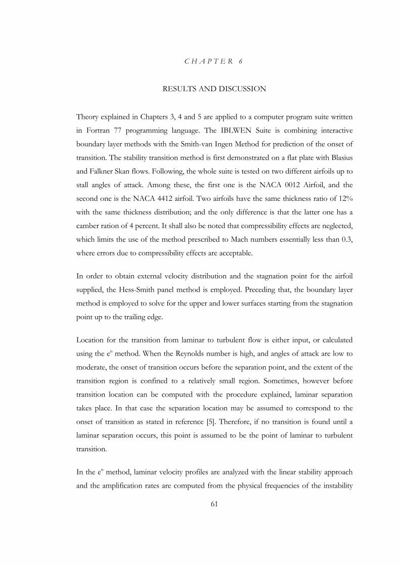
61

C H A P T E R 6

RESULTS AND DISCUSSION

Theory explained in Chapters 3, 4 and 5 are applied to a computer program suite written

in Fortran 77 programming language. The IBLWEN Suite is combining interactive

boundary layer methods with the Smith-van Ingen Method for prediction of the onset of

transition. The stability transition method is first demonstrated on a flat plate with Blasius

and Falkner Skan flows. Following, the whole suite is tested on two different airfoils up to

stall angles of attack. Among these, the first one is the NACA 0012 Airfoil, and the

second one is the NACA 4412 airfoil. Two airfoils have the same thickness ratio of 12%

with the same thickness distribution; and the only difference is that the latter one has a

camber ration of 4 percent. It shall also be noted that compressibility effects are neglected,

which limits the use of the method prescribed to Mach numbers essentially less than 0.3,

where errors due to compressibility effects are acceptable.

In order to obtain external velocity distribution and the stagnation point for the airfoil

supplied, the Hess-Smith panel method is employed. Preceding that, the boundary layer

method is employed to solve for the upper and lower surfaces starting from the stagnation

point up to the trailing edge.

Location for the transition from laminar to turbulent flow is either input, or calculated

using the en method. When the Reynolds number is high, and angles of attack are low to

moderate, the onset of transition occurs before the separation point, and the extent of the

transition region is confined to a relatively small region. Sometimes, however before

transition location can be computed with the procedure explained, laminar separation

takes place. In that case the separation location may be assumed to correspond to the

onset of transition as stated in reference [5]. Therefore, if no transition is found until a

laminar separation occurs, this point is assumed to be the point of laminar to turbulent

transition.

In the en method, laminar velocity profiles are analyzed with the linear stability approach

and the amplification rates are computed from the physical frequencies of the instability

62

waves as described in Chapter 4. When the n-factor, that is the integrated amplification

rate, reaches a value between 8 and 10 upon preference of the user, transition is assumed

to be found.

After the onset of transition is determined, the value is supplied to the program suite

externally and inviscid-viscous calculations are carried on to obtain the flow field around

the airfoil. Given an external velocity distribution, each boundary layer solution starting

form the stagnation point and ending in the wake region is called a sweep. After a number

of sweeps are accomplished, the blowing velocity distribution is found and is used to

obtain a new external velocity distribution using the Hess-Smith panel method. This

whole procedure including the updating of the external velocity distribution and doing

some number of sweeps is called a cycle. One must set the number of cycles to a high

enough value to ensure convergence.

Number of iterations

Cl

10 20 30 40 501

1.1

1.2

1.3

1.4

1.5

1.6

1.7

Value calculated at cycleConverged value

Figure 6.1 Convergence history for NACA 0012 Airfoil ( cR =6×106, α =12 ° )

63

While calculating the potential flow around the airfoil at high angles of attack (i.e. when a

separated zone exists near the trailing edge, one has to evaluate the velocities and supply

the Kutta condition at the edge of the displacement thickness as stated in references [1]

and [3]. On the other hand, even if this is the case, the blowing velocity distribution

obtained from the boundary layer solutions are applied on to the airfoil surface as

boundary conditions. An over relaxation scheme which is taken from the work done by

Özgen is applied in order to accelerate convergence. A sample convergence history plot is

given in figure 6.1. As seen in figure 6.1, after 20 cycles, one obtains the final converged

result.

6.1 Falkner Skan Flow

In order to demonstrate the transition prediction procedure, the en program was first run

using Falkner-Skan velocity profiles, for which after transformation of variables, velocity

profile is the same for all stations. Calculations are carried out for Falkner-Skan parameter

β which is defined in equation 6.1, ranging from -0.1988 to 0.5. Note that the parameter

m seen in equation 6.1 is the pressure gradient parameter.

21m

mβ =

+ (6.1)

e

e

dUxmU dx

= (6.2)

Neutral stability calculations agree very well with Özgen and Mack as in figure 6.2 given

for Blasius flow, which is a Falkner-Skan flow with no pressure gradient. Figures from 6.3

to 6.13 are the integrated amplification factor, n , plotted against the local Reynolds

number. It shall once again be emphasized that the local Reynolds number used is based

on the Falkner-Skan length scale, which is the square root of actual (i.e. non-transformed)

Reynolds number. One may easily notice that the transition location moves downstream

as the pressure gradient parameter increases, that is pressure gradient changes from

adverse to favorable. Values of the parameter β indicate an adverse pressure gradient if it

is less than zero, no gradient if it is equal to zero and a favorable pressure gradient if it is

greater than zero.

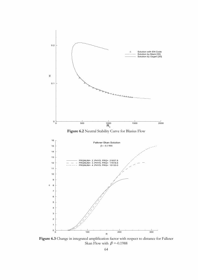
64

Rx

α

0 500 1000 1500 20000

0.1

0.2

Solution with EN CodeSolution by Mack [35]Solution by Ozgen [30]

Figure 6.2 Neutral Stability Curve for Blasius Flow

R

n

0 100 200 3000

1

2

3

4

5

6

7

8

9

10

11

12

13

14

15

16

FRQNUM= 2 ,PHYS. FRQ= 21837.6FRQNUM= 3 ,PHYS. FRQ= 17918.6FRQNUM= 4 ,PHYS. FRQ= 15133.0

Falkner-Skan Solutionβ=−0.1988

Figure 6.3 Change in integrated amplification factor with respect to distance for Falkner

Skan Flow with β =-0.1988

65

R

n

0 100 200 300 400 500 600 700 8000

1

2

3

4

5

6

7

8

9

10

11

12

13

14

15

16

FRQNUM= 2 ,PHYS. FRQ= 7595.01FRQNUM= 3 ,PHYS. FRQ= 6467.94FRQNUM= 4 ,PHYS. FRQ= 5638.31FRQNUM= 5 ,PHYS. FRQ= 5001.84FRQNUM= 6 ,PHYS. FRQ= 4497.93

Falkner-Skan Solutionβ=−0.15

Figure 6.4 Change in integrated amplification factor with respect to distance for Falkner

Skan Flow with β =-0.15

R

n

0 250 500 750 10000

1

2

3

4

5

6

7

8

9

10

11

12

13

FRQNUM= 2 ,PHYS. FRQ= 4270.79FRQNUM= 3 ,PHYS. FRQ= 2897.42FRQNUM= 4 ,PHYS. FRQ= 2216.37

Falkner-Skan Solutionβ=−0.1

Figure 6.5 Change in integrated amplification factor with respect to distance for Falkner

Skan Flow with β =-0.1

66

R

n

0 500 10000

1

2

3

4

5

6

7

8

9

10

11

FRQNUM= 2 ,PHYS. FRQ= 3555.20FRQNUM= 3 ,PHYS. FRQ= 2420.02FRQNUM= 4 ,PHYS. FRQ= 1858.14FRQNUM= 5 ,PHYS. FRQ= 1519.64FRQNUM= 6 ,PHYS. FRQ= 1292.08FRQNUM= 7 ,PHYS. FRQ= 1127.97

Falkner-Skan Solutionβ=−0.05

Figure 6.6 Change in integrated amplification factor with respect to distance for Falkner

Skan Flow with β =-0.05

R

n

0 200 400 600 800 1000 1200 1400 1600 1800 2000 22000

1

2

3

4

5

6

7

8

9

10

11

12

13

14

FRQNUM= 2 ,PHYS. FRQ= 1537.53FRQNUM= 3 ,PHYS. FRQ= 1185.55FRQNUM= 4 ,PHYS. FRQ= 972.682FRQNUM= 5 ,PHYS. FRQ= 829.118FRQNUM= 6 ,PHYS. FRQ= 725.284FRQNUM= 7 ,PHYS. FRQ= 646.437FRQNUM= 8 ,PHYS. FRQ= 584.375

Flakner-Skan Solution

β=0.0 (Blasius Flow)

Figure 6.7 Change in integrated amplification factor with respect to distance for Blasius

Flow

67

R

n

0 1000 2000 30000

1

2

3

4

5

6

7

8

9

10

11

12

13

14

FRQNUM= 2 ,PHYS. FRQ= 1140.20FRQNUM= 3 ,PHYS. FRQ= 876.443FRQNUM= 4 ,PHYS. FRQ= 718.014FRQNUM= 5 ,PHYS. FRQ= 611.512FRQNUM= 6 ,PHYS. FRQ= 534.631FRQNUM= 7 ,PHYS. FRQ= 476.322FRQNUM= 8 ,PHYS. FRQ= 430.459FRQNUM= 9 ,PHYS. FRQ= 393.369

Falkner-Skan Solutionβ=0.05

Figure 6.8 Change in integrated amplification factor with respect to distance for Falkner

Skan Flow with β =0.05

R

n

0 1000 2000 30000

1

2

3

4

5

6

7

8

9

10

11

12

13

FRQNUM= 2 ,PHYS. FRQ= 805.409FRQNUM= 3 ,PHYS. FRQ= 616.914FRQNUM= 4 ,PHYS. FRQ= 504.547FRQNUM= 5 ,PHYS. FRQ= 429.275FRQNUM= 6 ,PHYS. FRQ= 375.046FRQNUM= 7 ,PHYS. FRQ= 333.969

Falkner-Skan Solutionβ=0.1

Figure 6.9 Change in integrated amplification factor with respect to distance for Falkner

Skan Flow with β =0.1

68

R

n

0 1000 2000 3000 4000 50000

1

2

3

4

5

6

7

8

9

10

11

12

13

14

15

FRQNUM= 2 ,PHYS. FRQ= 411.643FRQNUM= 3 ,PHYS. FRQ= 333.983FRQNUM= 4 ,PHYS. FRQ= 282.788FRQNUM= 5 ,PHYS. FRQ= 246.241

Falkner-Skan Solutionβ=0.2

Figure 6.10 Change in integrated amplification factor with respect to distance for Falkner

Skan Flow with β =0.2

R

n

0 1000 2000 3000 4000 5000 6000 70000

1

2

3

4

5

6

7

8

9

10

11

12

13

14

15

16

17

18

19

20

21

22

23

24

FRQNUM= 6 ,PHYS. FRQ= 392.545FRQNUM= 7 ,PHYS. FRQ= 293.909FRQNUM= 8 ,PHYS. FRQ= 237.879FRQNUM= 9 ,PHYS. FRQ= 201.102

Falkner-Skan Solutionβ=0.3

Figure 6.11 Change in integrated amplification factor with respect to distance for Falkner

Skan Flow with β =0.3

69

R

n

0 1000 2000 3000 4000 5000 60000

1

2

3

4

5

6

7

8

9

10

11

12

13

14

15

16

FRQNUM= 2 ,PHYS. FRQ= 397.203FRQNUM= 5 ,PHYS. FRQ= 350.396FRQNUM= 7 ,PHYS. FRQ= 326.065FRQNUM= 9 ,PHYS. FRQ= 305.421FRQNUM= 11 ,PHYS. FRQ= 287.590FRQNUM= 13 ,PHYS. FRQ= 271.982

Falkner-Skan Solutionβ=0.4

Figure 6.12 Change in integrated amplification factor with respect to distance for Falkner

Skan Flow with β =0.4

R

n

0 1000 2000 3000 4000 5000 6000 70000

1

2

3

4

5

6

7

8

9

10

11

12

13

14

15

16

17

18

FRQNUM= 2 ,PHYS. FRQ= 395.027FRQNUM= 3 ,PHYS. FRQ= 366.453FRQNUM= 4 ,PHYS. FRQ= 342.910FRQNUM= 5 ,PHYS. FRQ= 322.868FRQNUM= 6 ,PHYS. FRQ= 305.463

Falkner-Skan Solutionβ=0.5

Figure 6.13 Change in integrated amplification factor with respect to distance for Falkner

Skan Flow with β =0.5

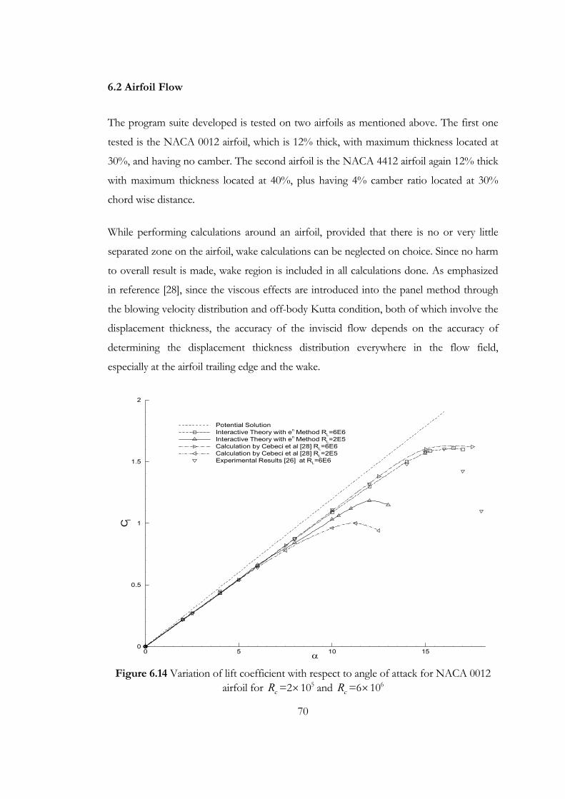
70

6.2 Airfoil Flow

The program suite developed is tested on two airfoils as mentioned above. The first one

tested is the NACA 0012 airfoil, which is 12% thick, with maximum thickness located at

30%, and having no camber. The second airfoil is the NACA 4412 airfoil again 12% thick

with maximum thickness located at 40%, plus having 4% camber ratio located at 30%

chord wise distance.

While performing calculations around an airfoil, provided that there is no or very little

separated zone on the airfoil, wake calculations can be neglected on choice. Since no harm

to overall result is made, wake region is included in all calculations done. As emphasized

in reference [28], since the viscous effects are introduced into the panel method through

the blowing velocity distribution and off-body Kutta condition, both of which involve the

displacement thickness, the accuracy of the inviscid flow depends on the accuracy of

determining the displacement thickness distribution everywhere in the flow field,

especially at the airfoil trailing edge and the wake.

α

Cl

0 5 10 150

0.5

1

1.5

2

Potential SolutionInteractive Theory with en Method RL=6E6Interactive Theory with en Method RL=2E5Calculation by Cebeci et al [28] RL=6E6Calculation by Cebeci et al [28] RL=2E5Experimental Results [26] at RL=6E6

Figure 6.14 Variation of lift coefficient with respect to angle of attack for NACA 0012

airfoil for cR =2×105 and cR =6×106

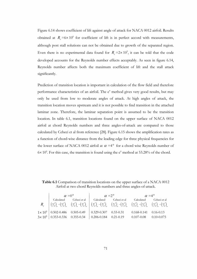
71

Figure 6.14 shows coefficient of lift against angle of attack for NACA 0012 airfoil. Results

obtained at cR =6×106 for coefficient of lift is in perfect accord with measurements,

although post stall solutions can not be obtained due to growth of the separated region.

Even there is no experimental data found for cR =2×105, it can be told that the code

developed accounts for the Reynolds number effects acceptably. As seen in figure 6.14,

Reynolds number affects both the maximum coefficient of lift and the stall attack

significantly.

Prediction of transition location is important in calculation of the flow field and therefore

performance characteristics of an airfoil. The en method gives very good results, but may

only be used from low to moderate angles of attack. At high angles of attack, the

transition location moves upstream and it is not possible to find transition in the attached

laminar zone. Therefore, the laminar separation point is assumed to be the transition

location. In table 6.1, transition locations found on the upper surface of NACA 0012

airfoil at chord Reynolds numbers and three angles-of-attack are compared to those

calculated by Cebeci et al from reference [28]. Figure 6.15 shows the amplification rates as

a function of chord-wise distance from the leading edge for three physical frequencies for

the lower surface of NACA 0012 airfoil at α =4° for a chord wise Reynolds number of

6×106. For this case, the transition is found using the en method at 53.28% of the chord.

Table 6.1 Comparison of transition locations on the upper surface of a NACA 0012 Airfoil at two chord Reynolds numbers and three angles-of-attack.

α =0° α =2° α =4° Calculated Cebeci et al Calculated Cebeci et al Calculated Cebeci et al

cR ( ) ( )tr tr

s xc c− ( ) ( )

tr trs xc c− ( ) ( )

tr trs xc c− ( ) ( )

tr trs xc c− ( ) ( )

tr trs xc c− ( ) ( )

tr trs xc c−

1×106 0.502-0.486 0.505-0.49 0.329-0.307 0.33-0.31 0.168-0.141 0.16-0.13 3×106 0.353-0.336 0.355-0.34 0.206-0.184 0.21-0.19 0.107-0.08 0.10-0.075

72

x/c

n

0 0.2 0.4 0.60

1

2

3

4

5

6

7

8

9

Physical Frequency = 4472.448 rad/sPhysical Frequency = 3638.217 rad/sPhysical Frequency = 2730.906 rad/s

Smith van-Ingen en Method Solution

Figure 6.15 Amplification rates calculated using the en method for lower surface of

NACA 0012 Airfoil at cR =6×106 and α =4 ° .

Figure 6.16 shows the variation of drag coefficient with respect to lift coefficient. Drag is

estimated using the formulation by Squire and Young [24] which is given below in

equation 6.3. In equation 6.5 the same formula is given in another form.

. . 52

. . . .2T EH

T E T Ed

uCc Uθ

+

∞

⎛ ⎞= ⎜ ⎟

⎝ ⎠ (6.3)

*. .

. .. .

T ET E

T E

H δθ

= (6.4)

2dC c

θ∞= (6.4)

In equation the terms . .T Eθ and . .T Eu are the momentum thickness and the edge velocity

at the trailing edge respectively. Free stream velocity is U∞ , while . .T EH is the shape factor

at the trailing edge and is defined in equation 6.4. In equation 6.5, the term θ∞ denotes

the momentum thickness at the far wake.

73

Cl

Cd

0 0.5 1 1.50

0.005

0.01

0.015

0.02

0.025

0.03

Interactive Theory with en Method RL=6E6Interactive Theory with en Method RL=2E5Experimental Results [26] at RL=6E6

Figure 6.16 Drag polar for NACA 0012 airfoil for cR =2×105 and cR =6×106

As seen in figure 6.16, the estimated drag value agrees well with the measurements except

for slight underestimation at moderate to high lift values. The maximum deviation is

observed at a lift coefficient value of 1.25 as 12.5%.

Given in figure 6.17 is the variation of displacement thickness at the trailing edge with

respect to the angle of attack. Notice that slope of the curve increases with increasing

angle of attack. At 17 degrees, the displacement thickness value reaches approximately

about 6% of the chord.

Figure 6.18 shows the viscous and inviscid pressure distribution. Since the area enclosed

by inviscid pressure distribution is slightly higher than the area enclosed by the viscous

one, the inviscid method overestimates the lift coefficient, as expected.

In figure 6.19, the displacement thickness distribution on the upper surface of the NACA

0012 airfoil at α =10° is shown. The displacement thickness first rises in the stream wise

direction until trailing edge and then falls as going towards the far wake.

74

α

δ∗

0 5 10 150

0.01

0.02

0.03

0.04

0.05

0.06

Figure 6.17 Variation of the displacement thickness with respect to angle of attack at the

trailing edge for NACA 0012 airfoil for cR =6×106

x/c

Cp

0 0.2 0.4 0.6 0.8 1

-10

-5

0

Potential SolutionInteractive Theory with en Method

Figure 6.18 Inviscid and viscous pressure distribution around NACA 0012 airfoil for

cR =6×106 at α =14°

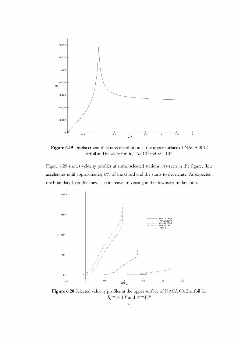
75

x/c

δ∗

0 0.5 1 1.5 2 2.5 3 3.5 40

0.002

0.004

0.006

0.008

0.01

0.012

0.014

Figure 6.19 Displacement thickness distribution at the upper surface of NACA 0012

airfoil and its wake for cR =6×106 and α =10°

Figure 6.20 shows velocity profiles at some selected stations. As seen in the figure, flow

accelerates until approximately 6% of the chord and the starts to decelerate. As expected,

the boundary layer thickness also increases traversing in the downstream direction.

u/Uo

η

-0.5 0 0.5 1 1.5 2 2.5

0

50

100

150

200

x/c=.007879x/c=.062610x/c=.441136x/c=.957467x/c=1.0

Figure 6.20 Selected velocity profiles at the upper surface of NACA 0012 airfoil for

cR =6×106 and α =15°

76

In figures 6.21 to 6.23, velocity profiles in the wake region are shown for NACA 0012

airfoil at cR =6×106 with angles of attack values of 0° , 8 ° and 15° respectively.

Velocity profiles for α =0 ° shown in figure 6.21 are perfectly symmetrical as expected.

One other important result is that the high velocity gradients no longer exist in the far

wake and are replaced by smooth gradients. At 3 chords downstream from the trailing

edge, where the calculations end, maximum deviation from the free stream velocity is

found to be approximately 5%. In figure 6.22, which is for α =8° , it is not possible to

mention about symmetry but the far wake velocity profiles are very close to the free

stream profile as expected.

Figure 6.23 shows the wake velocity profiles for α =15° . In this figure, flow at the lower

surface is laminar where the upper surface is turbulent. Moreover, the last 10% of the

flow is separated. Therefore the thickness of the boundary layer coming from the upper

surface is approximately 20 times larger than that of the lower surface. As desired, the two

velocity profiles merge and result in a free stream like velocity profile at the far wake.

u/Uo

η

0 0.1 0.2 0.3 0.4 0.5 0.6 0.7 0.8 0.9 1

-50

0

50 x/c=1.000000x/c=1.013303x/c=1.090166x/c=1.428687x/c=4.00000

η=0

Figure 6.21 Velocity profiles in the wake for NACA 0012 airfoil for cR =6×106 and

α =0°

77

u/Uo

η

0 0.1 0.2 0.3 0.4 0.5 0.6 0.7 0.8 0.9 1

-50

0

50

100

x/c=1.000000x/c=1.013626x/c=1.091757x/c=1.432677x/c=3.985334

η=0

Figure 6.22 Velocity profiles in the wake for NACA 0012 airfoil for cR =6×106 and

α =8°

u/Uo

η

-0.1 0 0.1 0.2 0.3 0.4 0.5 0.6 0.7 0.8 0.9 1

-100

0

100

200

x/c=1.000000x/c=1.014106x/c=1.094067x/c=1.437976x/c=3.950347

η=0

Figure 6.23 Velocity profiles in the wake for NACA 0012 airfoil for cR =6×106 and

α =15°

78

Given in figure 6.24 is the variation of surface friction coefficient with respect to distance

traversed in downstream direction measured from the stagnation point for upper surface

of the NACA 0012 airfoil with Reynolds number based on chord of 2×105. The jumps in

fC values show transition. fC values less than zero show separation. For α =12° ,

approximately 26% of the flow is separated. Also one may notice the laminar separation

taking place at s c=0.82 for α =0°

s/c

Cf

0 0.1 0.2 0.3 0.4 0.5 0.6 0.7 0.8 0.9 1 1.1-0.0025

0

0.0025

0.005

0.0075

0.01

α=0ο

α=6ο

α=8ο

α=10ο

α=12ο

Figure 6.24 Variation of drag surface friction coefficient against surface distance

traversed for NACA 0012 airfoil for cR =2×105

The other airfoil tested is the NACA 4412 airfoil with 4% of camber. The test were

carried out for cR =6×106 and for cR =2×105. Lift coefficient with respect to angle of

attack is plotted in figure 6.25. Again, the results obtained are in good accord with

measurements. Like in NACA 0012 airfoil, large separated regions on the upper surface at

high angles of attack prevent to find solutions for post stall cases.

79

Figure 6.26 shows variation of drag coefficient with respect to lift coefficient. For

moderate values of lift coefficient, a slight overestimation of drag coefficient is observed.

On the other hand for low and high values the values are slightly underestimated. Overall,

the drag polar is within acceptable values. Maximum deviation between measured

calculated values of drag coefficient is found to be 15%.

α

Cl

0 5 10 15

0

1

2

Potential SolutionInteractive Theory with en Method RL=6E6Interactive Theory with en Method RL=2E5Experimental Results at RL=6e6 [26] at RL=6E6

Figure 6.25 Variation of lift coefficient with respect to angle of attack for NACA 4412

airfoil for cR =2×105 and cR =6×106

Given in figure 6.27 is the variation of surface friction coefficient with respect to distance

traversed in downstream direction measured from the stagnation point for upper surface

of the NACA 4412 airfoil with Reynolds number based on chord of 2×105. The jumps in

fC values show transition. fC values less than zero show separation. For α =12° ,

approximately 32% of the flow is separated. Also one may notice the laminar separation

taking place at s c=0.16 for α =12°

80

Cl

Cd

0 0.5 1 1.50

0.005

0.01

0.015

0.02

0.025

0.03

Interactive Theory with en Method RL=6E6Interactive Theory with en Method RL=2E5Experimental Results ar RL=6E6 [26]

Figure 6.26 Drag polar for NACA 4412 airfoil for cR =2×105 and cR =6×106

s/c

Cf

0.1 0.2 0.3 0.4 0.5 0.6 0.7 0.8 0.9 1 1.1-0.0025

0

0.0025

0.005

0.0075

α=0ο

α=6ο

α=8ο

α=10ο

α=12ο

Figure 6.27 Variation of drag surface friction coefficient against surface distance

traversed for NACA 4412 airfoil for cR =2×105

81

C H A P T E R 7

CONCLUSION

In this study, Smith-van Ingen transition prediction procedure is implemented into the

previous study carried out by Özgen. The resultant program suite is tested for Falkner

Skan flows and two airfoils. For airfoil solutions, the results are in good accord with

measurements until the stall angle of attack.

At high angles of attack, due the growth of the boundary layer and the displacement

thickness, constant pressure assumption across the boundary layer becomes less accurate.

Due to this reason and excessive separated regions in the flow, post stall solutions can not

be performed.

In this study, Cebeci-Smith algebraic turbulence model is used. Any empirical model

which formulated the turbulent viscosity may easily be implemented to the computer

program. On the other hand, in order to solve for largely separated flows, employment of

a higher order turbulence model may be more suitable.

As stated in reference [1], determination of transition plays a key role in obtaining correct

solutions. Implementing a more concrete physical means to calculate transition was aimed

in this study. For moderate Reynolds numbers, results show that use of Smith-van Ingen

transition prediction procedure does not bring much compared to empirical correlations

such as Michel’s formula. On the other hand, it proved to be useful for low Reynolds

numbers where Michel’s formula failed. Since the en transition prediction method is valid

for both incompressible and compressible flows, its applicability ranges from low to high

Reynolds numbers where empirical correlations are not valid. Another advantage is that en

transition procedure used in this study may easily be extended to three dimensional flows

without much effort, where in such a case using such a method is essential since no

empirical correlation is present for 3D flows.

In terms of computational time, solving for a single angle of attack varies from 3 to 8

minutes depending on the value of angle of attack. Time required increases with

82

increasing angle-of attack. The reasoning for this is that separated flows require much

more cycles to be done and also it is necessary to use the Homotopy continuation method

for largely separated flows which also requires additional computational time. However,

compared to thin-layer Navier Stokes solutions, this method is much faster and therefore

proves that it is useful.

The computer program presented in this study currently applies to single element airfoils

with incompressible flows. In the future, modifications such as adding the ability of

solving flow around multi-element airfoils, including compressibility effects or making the

program suite able to handle three dimensional flows may be done. The author hopes that

this study may be a reliable basis for such studies.

83

BIBLIOGRAPHY

[1] Serkan Özgen. “INTERACTIVE BOUNDARY LAYER CALCULATION OVER AN AIRFOIL AND ITS RESULTING WAKE”, Master’s Thesis, Middle East Technical University, Ankara, 1994.

[2] K.C. Chang, N. Alemdaroğlu, U. Mehta, T. Cebeci. “FURTHER COMPARISONS OF INTERACTIVE BOUNDARY LAYER AND THIN-LAYER NAVIER STOKES PROCEDURES”, Journal of Aircraft 25/10, 897-903, AIAA, 1988

[3] T. Cebeci, R.W. Clark, K.C. Chang, N.D. Halsey, K. Lee. “AIRFOILS WITH SEPARATION AND THE RESULTING WAKES”, Journal of Fluid Mechanics, 163, 323-247, 1986.

[4] T. Cebeci, J. Jau, D. Vitiello, K.C. Chang. “PREDICTION OF POST STALL FLOWS ON AIRFOILS”, 4th Symposium on Numerical and Physical Aspects of Aerodynamic Flows, California State University, Long Beach, 1989

[5] T. Cebeci, J. Cousteix. “MODELING AND COMPUTATION OF BOUNDARY LAYER FLOWS”, Springer Verlag, New York, 1999

[6] J. D. Anderson. “FUNDAMENTALS OF AERODYNAMICS”, McGraw Hill, 1991

[7] H.N. Alemdaroğlu. “NUMERICAL SOLUTIONS OF BOUNDARY LAYER EQUATIONS”, Lecture Series Presented at School of Aeronautics and Astronautics, İstanbul Technical University, 1990

[8] T. Cebeci, P. Bradshaw. “PHYSICAL AND COMPUTATIONAL ASPECTS OF CONVECTIVE HEAT TRANSFER”, Springer Verlag, New York, 1984

[9] J.A. Schetz. “FOUNDATIONS OF BOUNDARY LAYER THEORY”, Prentice Hall Inc., New Jersey, 1984

[10] H.B. Keller. “A NEW DIFFERENCE SCHEME FOR PARABOLIC PROBLEMS IN NUMERICAL SOLUTION OF PARTIAL DIFFERENTIAL EQUATIONS VOLUME II”, Academic, New York, 1970

[11] T. Cebeci. “AN ENGINEERING APPROACH TO THE CALCULATION OF AERODYNAMIC FLOWS”, Springer Verlag, New York, 1999

[12] T. Cebeci. “CALCULATION OF MULTI-ELEMENT AIRFOILS AND WINGS AT HIGH LIFT”, 71st Fluid Dynamics Panel Meeting, Banff-Alberta Canada, 1992.

84

[13] T. Cebeci S.M. Schimke. “THE CALCULATION OF SEPARATION BUBBLES IN INTERACTIVE TURBULENT BOUNDARY LAYERS”, Journal of Fluid Mechanics, 131, 305-317, 1983

[14] T. Cebeci. “ESSENTIAL INGREDIENTS OF A METHOD FOR LOW REYNOLDS NUMBER AIRFOILS”, AIAA Journal, 26, 1680-1688, 1989

[15] A.E.P. Veldman. “NEW, QUASI-SIMULTANEOUS METHOD TO CALCULATE INTERACTING BOUNDARY LAYERS”, AIAA Journal, 154, 79-84, 1981

[16] A.G. Hansen. “SIMILARITY ANALYSIS OF BOUNDARY VALUE PROBLEMS IN ENGINEERING”, Prentice Hall Inc., New Jersey, 1964

[17] S. Özgen. “LECTURE NOTES OF AE549: LINEAR STABILITY THEORY AND LAMINAR TO TURBULENT BOUNDARY LAYER TRANSITION”, Middle East Technical University, Ankara, 2004

[18] L. M. Mack. “BOUNDARY LAYER LINEAR STABILITY THEORY”, Special Course on Stability and Transition of Laminar Flow, AGARD No.84-33757, p.23-34, 1984

[19] T. Cebeci., J.P. Shao, H.H. Chen, K.C. Chang. “THE PREFERRED APPROACH FOR CALCULATING TRANSITION BY STABILITY THEORY”, International Conference on Boundary and Interior Layers – Computational and Asymptotic Methods, ONERA Centre de Toulouse, 2004

[20] T. Herbert. “PARABOLIZED STABILITY EQUATIONS”, Special Course on Progress in Transition Modeling, AGARD Rep. No. 793, 1994

[21] T. Cebeci, A.M.O. Smith., “ANALYSIS OF TURBULENT BOUNDARY LAYERS”, Academic, New York, 1974

[22] K.C. Chang, M.N. Bui, T. Cebeci, J.H. Whitelaw. “THE CALCULATION OF TURBULENT WAKES”, AIAA Journal, 24, 200, 1986

[23] T. Cebeci, K.C. Chang, C. Li, J.H. Whitelaw. “TURBULENCE MODELS FOR WALL BOUNDARY LAYERS”, AIAA Journal, 24, 359-360, 1986

[24] R.L. Simpson, Y.T. Chew, B.G. Shivaprasad. “THE STRUCTURE OF A SEPARATING TURBULENT BOUNDARY LAYER. PART 1. MEAN FLOW AND REYNOLDS STRESS”, Journal of Fluid Mechanics, 113, 1981

[25] M.R. Head., “EDDY VISCOSITY IN TURBULENT BOUNDARY LAYERS”, Aero. Quart., 27, 200, 1976

85

[26] A. Nakayama. “MEASUREMENTS IN THE BOUNDARY LAYER AND WAKE OF TWO AIRFOIL MODELS”, Douglas Aircraft Company, Report No. MDC J2403, Long Beach, California, 1982

[27] T. Cebeci, P. Bradshaw. “MOMENTUM TRANSFER IN BOUNDARY LAYERS”, Hemisphere Publishing Co., Washington, 1977

[28] U. Mehta, K.C. Chang, T. Cebeci. “RELATIVE ADVANTAGES OF THIN-LAYER NAVIER-STOKES AND INTERACTIVE BOUNDARY LAYER PROCEDURES”, Numerical and Physical Aspects of Aerodynamic Flow III, Springer Verlag, New York, 1986.

[29] J. Moran. “AN INTRODUCTION TO THEORETICAL AND COMP-UTATIONAL AERODYNAMICS”, John Wiley and Sons, New York, 1984

[30] R. Michel. “ETUDE DE LA TRANSITION SUR LES PROFILES D’AILE; ESTABLISHEMENT D’UN CRITÈRE DE DETERMINATION DE POINT DE TRANSITION ET CALCUL DE LA TRINEE DE PROFILE INCOMPRESSIBLE”, ONERA Rept. 1/1578A, 1951

[31] W.J. Duncan. A.S. Thom, A.D. Young. “MECHANICS OF FLUIDS”, Arnold, London, 1970

[32] I.H. Abott, A.E. von Doenhoff. “THEORY OF WING SECTIONS”, Dover Publications, New York, 1959

[33] S. Özgen, H.N. Alemdaroğlu. “KANAT PROFILI ÜZERINDE ART-İZ BÖLGESINDE SINIR TABAKASININ ETKILEŞIMLI OLARAK HESAPLANMASI”, 1. Havacılık Sempozyumu, İstanbul, Turkey, 1994

[34] H. Dumitrescu, V. Cardo. “AN INTERACTIVE BOUNDARY LAYER FOR AIRFOILS”, Proceedings of the Romanian Academy, Series A, Volume 3, No:1-2, 2002

[35] K.C. Chang. “Computational Fluid Dynamics Tool Development and Validation – A General Interactive Boundary-Layer Method for Three Dimensional Flows”, California State University, Long Beach, 2001

86

A P P E N D I X A

BLOCK ELIMINATION METHOD

To solve the system constructed above in sub-section 3.2.2, a technique called the block

elimination method is used. The method is explained in detail in references [7],[8] and

[27]. The method is analogous to the Gaussian elimination technique.

First step is to decompose the coefficient matrix [ ]A , into lower and upper triangular

matrices as:

[ ] { } { }A rδ⋅ = (3.38)

[ ] [ ] { } { } . L U rδ = (A.1)

The tri-diagonal coefficient matrix can be written as:

0 0

1 1 1 1 1 1

2 2 2 2

1 1 1 1 1 1

0 0 0 0 0 00 0 0

0 0 00 0 0 0 0 0

o o

j j j j j j

J J J J J J

J J J J

I C A CI C B A C

I B A C

I C B A C

I C B A CI B A

− − − − − −

∆⎡ ⎤ ⎡ ⎤ ⎡ ⎤⎢ ⎥ ⎢ ⎥ ⎢ ⎥Γ ∆⎢ ⎥ ⎢ ⎥ ⎢ ⎥⎢ ⎥ ⎢ ⎥ ⎢ ⎥Γ⎢ ⎥ ⎢ ⎥ ⎢ ⎥⎢ ⎥ ⎢ ⎥ ⎢ ⎥=⎢ ⎥ ⎢ ⎥ ⎢Γ ∆⎢ ⎥ ⎢ ⎥ ⎢⎢ ⎥ ⎢ ⎥ ⎢⎢ ⎥ ⎢ ⎥ ⎢Γ ∆⎢ ⎥ ⎢ ⎥ ⎢

Γ ∆⎢ ⎥ ⎢ ⎥ ⎢⎣ ⎦ ⎣ ⎦ ⎣ ⎦

⎥⎥⎥⎥⎥⎥

(A.2)

Where I is the identity matrix. The solution procedure consists of two major steps: the

forward sweep and the backward sweep.

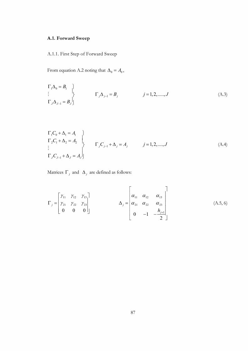
87

A.1. Forward Sweep

A.1.1. First Step of Forward Sweep

From equation A.2 noting that 0 0A∆ = ,

1 0 1

1J J J

B

B−

Γ ∆ = ⎫⎪⎬⎪Γ ∆ = ⎭

1j j jB−Γ ∆ = 1,2,.....,j J= (A.3)

1 0 1 1

2 1 2 2

1J J J J

C AC A

C A−

Γ + ∆ = ⎫⎪Γ + ∆ = ⎪⎬⎪⎪Γ + ∆ = ⎭

1j j j jC A−Γ + ∆ =

1,2,....,j J= (A.4)

Matrices jΓ and j∆ are defined as follows:

11 12 13

21 22 23

0 0 0j

γ γ γγ γ γ⎡ ⎤⎢ ⎥Γ = ⎢ ⎥⎢ ⎥⎣ ⎦

11 12 13

21 22 23

10 12

j

jh

α α αα α α

+

⎡ ⎤⎢ ⎥⎢ ⎥

∆ = ⎢ ⎥⎢ ⎥⎢ ⎥− −⎣ ⎦

(A.5, 6)

88

A.1.2. Second Step of Forward Sweep

Letting:

{ } [ ] { }w U δ= ⋅ (A.7)

equation A.1 becomes:

[ ] { } { }L w r⋅ = (A.8)

or:

0 0

1 1 1

2

0 00

00 0

j j j

J J J

I w rI w r

I

I w r

I w r

⎡ ⎤ ⎧ ⎫ ⎧ ⎫⎢ ⎥ ⎪ ⎪ ⎪ ⎪Γ⎢ ⎥ ⎪ ⎪ ⎪ ⎪⎢ ⎥ ⎪ ⎪ ⎪ ⎪Γ⎢ ⎥ ⎪ ⎪ ⎪ ⎪

⎪ ⎪ ⎪ ⎪⎢ ⎥ =⎨ ⎬ ⎨ ⎬⎢ ⎥Γ ⎪ ⎪ ⎪ ⎪⎢ ⎥ ⎪ ⎪ ⎪ ⎪⎢ ⎥ ⎪ ⎪ ⎪ ⎪⎢ ⎥ ⎪ ⎪ ⎪ ⎪⎢ ⎥ ⎪ ⎪ ⎪ ⎪Γ⎢ ⎥⎣ ⎦ ⎩ ⎭ ⎩ ⎭

(A.9)

From the above expression:

0 0w r=

1 0 1 1

2 1 2 2

1 J J J J

w w rw w r

w w r−

Γ + = ⎫⎪Γ + = ⎪⎬⎪⎪Γ + = ⎭

1jj j jw r w −= −Γ 1,2,.....,j J= (A.10)

All the terms on the right hand side of the above equation are known so jw vectors can

be easily found. With this, the forward sweep is completed.

89

A.2. Backward Sweep

Recalling:

{ } [ ] { }w U δ= ⋅ (A.11)

or:

0 0 0 0

1 1 1 1

1

0 00

00 0

j j j j

J

J J J

C wC w

C w

Cw

δδ

δ

δ−

∆⎡ ⎤ ⎧ ⎫ ⎧ ⎫⎢ ⎥ ⎪ ⎪ ⎪ ⎪∆⎢ ⎥ ⎪ ⎪ ⎪ ⎪⎢ ⎥ ⎪ ⎪ ⎪ ⎪⎢ ⎥ ⎪ ⎪ ⎪ ⎪

⎪ ⎪ ⎪ ⎪⎢ ⎥ =⎨ ⎬ ⎨ ⎬⎢ ⎥∆ ⎪ ⎪ ⎪ ⎪⎢ ⎥ ⎪ ⎪ ⎪ ⎪⎢ ⎥ ⎪ ⎪ ⎪ ⎪⎢ ⎥ ⎪ ⎪ ⎪ ⎪⎢ ⎥ ⎪ ⎪ ⎪ ⎪∆⎢ ⎥⎣ ⎦ ⎩ ⎭ ⎩ ⎭

(A.12)

From the above expression:

J J Jwδ∆ =

1 1 1 1

0 0 0 1 0

J J J J JC w

C w

δ δ

δ δ

− − − −∆ + = ⎫⎪⎬⎪∆ + = ⎭

1j j j j jw Cδ δ +∆ = − 1, 2,....,0j J J= − − (A.13)

In the above expression, everything except the jδ vector is known, so it is easy to extract

jδ . In this way, the perturbation quantities which are searched for are solved. This step

completes the block elimination method.

90

A P P E N D I X B

APPROXIMATION OF THE HILBERT INTEGRAL

Recalling the definition of the Hilbert integral:

( )1

1( ) ( )Lx

e iix

dU x Gxξδ ξ

π ξ=

−∫ (B.1)

Where ( ) dFGd

ξξ

= , and ( )*e

iF U δ= .

Where ξ is a dummy variable over the integration range 1 Lx xξ≤ ≤ within ix is

confined. Over each subinterval ( )1,k kx x− , ( )G ξ will be approximated by its midpoint

value:

( ) ( )1

11/ 2 ln

k

k

xi k

ki i kx

x xdG Gx x xξξξ

−

−−

⎡ ⎤−= ⎢ ⎥− −⎣ ⎦

∫ (B.2)

where:

11/ 2

11/ 2

k kk

k kk

F FdFGd x xξ

−−

−−

⎛ ⎞ −= =⎜ ⎟ −⎝ ⎠

(B.3)

Replacing 1/ 2kG − by its equivalent expression given by equation B.3, equation B.2 can be

written as:

( ) ( )1

1 1

1

lnk

k

xk k i k

i k k i kx

F F x xdGx x x x xξξξ

−

− −

−

⎡ ⎤− −= ⎢ ⎥− − −⎣ ⎦

∫ (B.4)

91

Letting:

( ) 1 11 ln i k

k k ki k

x xE x xx x

− −−

⎡ ⎤−= − ⎢ ⎥−⎣ ⎦

(B.5)

equation B.4 can be further written as:

( ) ( ) ( ) ( )1

* *1 1

k

k

x

e ek k k k k kix

dF d F F E E U Ud x

ξ δ δξ ξ

−

− −⎡ ⎤= − = −⎣ ⎦−∫ (B.6)

Within the subinterval ( ) ( )1 , 1i i− +⎡ ⎤⎣ ⎦ , the calculation will be performed assuming a

linear variation of ( )G ξ as:

( ) ( )iG A x Bξ ξ= − + (B.7)

Then:

( ) 11/ 2 2

i ii i

x xG x A x Bξ −−

+⎛ ⎞= = − +⎜ ⎟⎝ ⎠

(B.8a)

1-1/ 2 2

i ii

x xG A B− −⎛ ⎞= +⎜ ⎟⎝ ⎠

(B.8b)

and in the same manner, 1/ 2iG + can be written as:

11/ 2 2

i ii

x xG A B++

−⎛ ⎞= +⎜ ⎟⎝ ⎠

(B.9)

Solving for A and B :

( )-1/ 2 1/ 2

1 1

2 i i

i i

G GA

x x+

− +

−=

− (B.10)

92

( ) ( )1/ 2 1 1/ 2 1

1 1

i i i i i i

i i

G x x G x xB

x x+ − − +

+ −

− − + −=

− (B.11)

Hence equation B.7 can be written as:

( ) ( )( ) ( ) ( ) ( )

( )1/ 2 1/ 2 1/ 2 1 1/ 2 1

1 1 1 1

2 i i i i i i i ii

i i i i

G G G x x G x xG x

x x x xξ ξ+ − + − − +

+ − + −

− − − + −= − +

− − (B.12)

So the expression for the Hilbert Integral becomes:

( ) ( ) ( ) ( )( ) ( )

( )( ) ( )

11

11

1

1

11/ 2 1/ 2 1/ 2

! 1

11/ 2

1 1

2 ln

ln

ii

ii

i

i

xxi i

i i i i xi i ix

xi ii i x

i i

x xdG G G G xx x x

x xG x

x x

ξξ ξξ

ξ

++

−−

+

−

−+ − +

+ −

+−

+ −

−= − − − −

− −

−− −

−

∫

( ) ( ) ( ) ( ) ( )( )

1

1

1/ 2 1 1/ 2 1 11/ 2 1/ 2

1 1 1

2 lni

i

xi i i i i i i i

i ii i i i ix

G x x G x x x xdG G Gx x x x xξξξ

+

−

+ − − + −+ −

+ − +

⎡ ⎤− + − ⎡ ⎤−= − − + ⎢ ⎥ ⎢ ⎥− − −⎣ ⎦⎣ ⎦

∫ (B

.13)

Now, G can be expressed in terms of /dF dξ :

11/ 2

11/ 2

i ii

i ii

F FdFGd x xξ

++

++

⎛ ⎞ −= =⎜ ⎟ −⎝ ⎠

11/ 2

11/ 2

i ii

i ii

F FdFGd x xξ

−−

−−

⎛ ⎞ −= =⎜ ⎟ −⎝ ⎠

(B.14, 15)

Equation B.13 can be written as:

( ) ( )( )( )

( )( )

( )( )

( )( )

1

1

1 11 1 1

1 1 1 1 1 1

1 1

1 1 1

2 ln

i

i

xi i i ii i i i i i

i i i i i i i i i i ix

i i i i

i i i i

F F x xF F F F x xdGx x x x x x x x x x x

F F x xx x x x

ξξξ

+

−

+ −+ − −

+ − + + − +

− +

− + −

− −⎡ ⎤− − −= − − +⎢ ⎥− − − − − −⎣ ⎦

− −+

− −

∫

1

1

ln i i

i i

x xx x

−

+

−−

(B.16)

Let ( )( )( ) ( )

1 1

1 1 1 1 1

2lni ii i ii

i i i i i i i i

x x x xEx x x x x x x x

+ −

− + − + −

− −= +

− − − − (B.17)

93

And ( )( )( ) ( )

1 11

1 1 1 1 1

2lni ii i ii

i i i i i i i i

x x x xEx x x x x x x x

− −+

+ + − + +

− −= −

− − − − (B.18)

Therefore, Hilbert Integral can be approximated by the formula:

( ) ( ) ( ) ( )( ) ( )

2 2 1 3 3 2 1 1 2 1

2 1 2 3 2 1 1

..........

..........

i i i iL L L L L L

i i i i i iL L L L L

Hi E F F E F F E F F E F F

E F E E F E E F E F− − − −

− −

= − + − + + − + −

= − + − + + − + (B.19)

and 1 0i ii LE E += = .

The coefficients ijC are now defined as:

( )11 i i

ij j jC E Eπ += − and *( ) ( )ej j jF x U xδ= (B.19, 20)

Recalling that ieU can be written as:

1i i

Noe e ij j

j

U U C D=

= +∑ (B.22)

where ijC as defined above and *ejD U δ= . In this form equation B.22 provides a

boundary condition which represents the viscous/inviscid interaction. It can be

generalized to the form:

( ) ( )* *

1

( ) ( )N

e e e eij j jj

U x U x C U Uκκ

δ δ=

⎡ ⎤= + −⎢ ⎥⎣ ⎦∑ (B.23)

where ( )eU xκ

corresponds to the inviscid velocity distribution which contains the

displacement thickness effect ( )* κδ coming from the previous iteration κ .

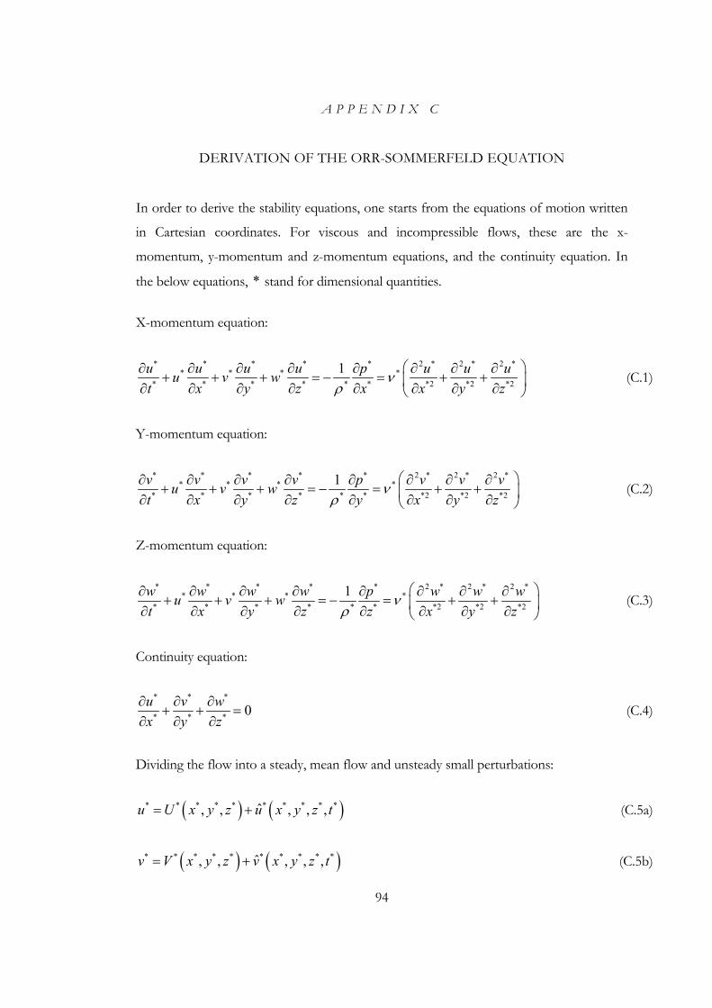
94

A P P E N D I X C

DERIVATION OF THE ORR-SOMMERFELD EQUATION

In order to derive the stability equations, one starts from the equations of motion written

in Cartesian coordinates. For viscous and incompressible flows, these are the x-

momentum, y-momentum and z-momentum equations, and the continuity equation. In

the below equations, * stand for dimensional quantities.

X-momentum equation:

* * * * * 2 * 2 * 2 ** * * *

* * * * * * *2 *2 *2

1u u u u p u u uu v wt x y z x x y z

νρ

⎛ ⎞∂ ∂ ∂ ∂ ∂ ∂ ∂ ∂+ + + = − = + +⎜ ⎟∂ ∂ ∂ ∂ ∂ ∂ ∂ ∂⎝ ⎠

(C.1)

Y-momentum equation:

* * * * * 2 * 2 * 2 ** * * *

* * * * * * *2 *2 *2

1v v v v p v v vu v wt x y z y x y z

νρ

⎛ ⎞∂ ∂ ∂ ∂ ∂ ∂ ∂ ∂+ + + = − = + +⎜ ⎟∂ ∂ ∂ ∂ ∂ ∂ ∂ ∂⎝ ⎠

(C.2)

Z-momentum equation:

* * * * * 2 * 2 * 2 ** * * *

* * * * * * *2 *2 *2

1w w w w p w w wu v wt x y z z x y z

νρ

⎛ ⎞∂ ∂ ∂ ∂ ∂ ∂ ∂ ∂+ + + = − = + +⎜ ⎟∂ ∂ ∂ ∂ ∂ ∂ ∂ ∂⎝ ⎠

(C.3)

Continuity equation:

* * *

* * * 0u v wx y z∂ ∂ ∂

+ + =∂ ∂ ∂

(C.4)

Dividing the flow into a steady, mean flow and unsteady small perturbations:

( ) ( )* * * * * * * * * *ˆ, , , , ,u U x y z u x y z t= + (C.5a)

( ) ( )* * * * * * * * * *ˆ, , , , ,v V x y z v x y z t= + (C.5b)

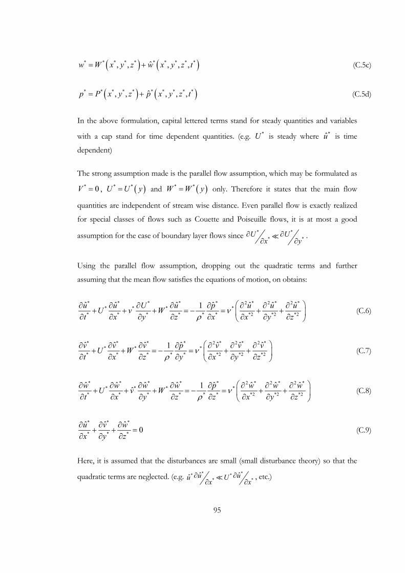
95

( ) ( )* * * * * * * * * *ˆ, , , , ,w W x y z w x y z t= + (C.5c)

( ) ( )* * * * * * * * * *ˆ, , , , ,p P x y z p x y z t= + (C.5d)

In the above formulation, capital lettered terms stand for steady quantities and variables

with a cap stand for time dependent quantities. (e.g. *U is steady where *u is time

dependent)

The strong assumption made is the parallel flow assumption, which may be formulated as * 0V = , ( )* *U U y= and ( )* *W W y= only. Therefore it states that the main flow

quantities are independent of stream wise distance. Even parallel flow is exactly realized

for special classes of flows such as Couette and Poiseuille flows, it is at most a good

assumption for the case of boundary layer flows since * ** *

U Ux y

∂ ∂∂ ∂

.

Using the parallel flow assumption, dropping out the quadratic terms and further

assuming that the mean flow satisfies the equations of motion, on obtains:

* * * * * 2 * 2 * 2 ** * * *

* * * * * * *2 *2 *2

ˆ ˆ ˆ ˆ ˆ ˆ ˆ1u u U u p u u uU v Wt x y z x x y z

νρ

⎛ ⎞∂ ∂ ∂ ∂ ∂ ∂ ∂ ∂+ + + = − = + +⎜ ⎟∂ ∂ ∂ ∂ ∂ ∂ ∂ ∂⎝ ⎠

(C.6)

* * * * 2 * 2 * 2 ** * *

* * * * * *2 *2 *2

ˆ ˆ ˆ ˆ ˆ ˆ ˆ1v v v p v v vU Wt x z y x y z

νρ

⎛ ⎞∂ ∂ ∂ ∂ ∂ ∂ ∂+ + = − = + +⎜ ⎟∂ ∂ ∂ ∂ ∂ ∂ ∂⎝ ⎠

(C.7)

* * * * * 2 * 2 * 2 ** * * *

* * * * * * *2 *2 *2

ˆ ˆ ˆ ˆ ˆ ˆ ˆ ˆ1ˆw w w w p w w wU v Wt x y z z x y z

νρ

⎛ ⎞∂ ∂ ∂ ∂ ∂ ∂ ∂ ∂+ + + = − = + +⎜ ⎟∂ ∂ ∂ ∂ ∂ ∂ ∂ ∂⎝ ⎠

(C.8)

* * *

* * *

ˆ ˆ ˆ0u v w

x y z∂ ∂ ∂

+ + =∂ ∂ ∂

(C.9)

Here, it is assumed that the disturbances are small (small disturbance theory) so that the

quadratic terms are neglected. (e.g. * ** ** *

ˆ ˆˆ u uu Ux x∂ ∂

∂ ∂, etc.)

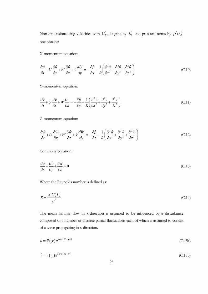
96

Non-dimensionalizing velocities with *RU , lengths by *

RL and pressure terms by 2* *RUρ

one obtains:

X-momentum equation:

2 2 2

2 2 2

ˆ ˆ ˆ ˆ ˆ ˆ ˆ1ˆu u u dU p u u uU W vt x z dy x R x y z

⎛ ⎞∂ ∂ ∂ ∂ ∂ ∂ ∂+ + + = − − + +⎜ ⎟∂ ∂ ∂ ∂ ∂ ∂ ∂⎝ ⎠

(C.10)

Y-momentum equation:

2 2 2

2 2 2

ˆ ˆ ˆ ˆ ˆ ˆ ˆ1v v v p v v vU Wt x z y R x y z

⎛ ⎞∂ ∂ ∂ ∂ ∂ ∂ ∂+ + = − − + +⎜ ⎟∂ ∂ ∂ ∂ ∂ ∂ ∂⎝ ⎠

(C.11)

Z-momentum equation:

2 2 2

2 2 2

ˆ ˆ ˆ ˆ ˆ ˆ ˆ1ˆw w w dW p w w wU W vt x z dy z R x y z

⎛ ⎞∂ ∂ ∂ ∂ ∂ ∂ ∂+ + + = − − + +⎜ ⎟∂ ∂ ∂ ∂ ∂ ∂ ∂⎝ ⎠

(C.12)

Continuity equation:

ˆ ˆ ˆ0u v w

x y z∂ ∂ ∂

+ + =∂ ∂ ∂

(C.13)

Where the Reynolds number is defined as:

* * *

*R RU LR ρ

µ= (C.14)

The mean laminar flow in x-direction is assumed to be influenced by a disturbance

composed of a number of discrete partial fluctuations each of which is assumed to consist

of a wave propagating in x-direction.

( ) ( )ˆ i x z tu u y e α β ω+ −= (C.15a)

( ) ( )ˆ i x z tv v y e α β ω+ −= (C.15b)

97

( ) ( )ˆ i x z tw w y e α β ω+ −= (C.15c)

( ) ( )ˆ i x z tp p y e α β ω+ −= (C.15d)

In the above equation C.15, ( )u y , ( )v y , ( )w y and ( )p y are the disturbance

amplitude functions with:

α : Wave number in x-direction and 2πα λ= with λ being the wavelength.

β : Wave number is z-direction.

ω : Circular frequency (complex) as r iiω ω ω= + .

The term rω in the above definition is the frequency and iω is the amplification rate.

Substituting the above relations into equations of motion, one obtains equations C.16-19

which are given below with primes denoting y∂∂

or d dy .

X-momentum equation:

( )2 21i u Ui u Wi u vU i p u u uRω α β α α β′ ′′− + + + = − + − + − (C.16)

Y-momentum equation:

( )2 21i v Ui v Wi v p v v vRω α β α β′′− + + = + − + − (C.17)

Z-momentum equation:

( )2 21i w Ui w Wi w i p w w wRω α β β α β′′− + + = − + − + − (C.18)

Continuity equation:

0i u v i wα β′+ + = (C.19)

98

Now with D denoting y∂∂

or d dy and rearranging terms, one obtainsthe following

system of equations:

( ) ( )2 2 21DUv i U W u i p D uRα β ω α α β⎡ ⎤+ + − = − + − +⎣ ⎦ (C.20)

( ) ( )2 2 21 i U W v p D vRα β ω α β⎡ ⎤′+ − = − + − +⎣ ⎦ (C.21)

( ) ( )2 2 21DWv i U W w i p D wRα β ω β α β⎡ ⎤+ + − = − + − +⎣ ⎦ (C.22)

( ) 0i u w Dvα β+ + = (C.23)

The boundary conditions for the above system of equations are given below in equation

C.24.

( ) ( ) ( )0 0 0 0u v w= = = at 0y = (no slip) (C.24a)

0u → , 0v → , 0w→ as y→∞ (free stream) (C.24b)

C.1. Reduction to a fourth order system

Multiplying the x-momentum equation by α , and z-momentum equation by β , and

adding them, one obtains the following equation after rearranging.

( )( ) ( ) ( )( ) ( )

2 2

2 2 21

i U W u w DU DW v i p

D u wR

α β ω α β α β α β

α β α β

+ − + + + = − +

⎡ ⎤+ − + +⎣ ⎦ (C.25)

Multiplying the x-momentum equation by β and subtracting the resultant from z-

momentum equation multiplied with α , one obtains equation C.26.

( )( ) ( ) ( ) ( )2 2 21i U W w u DW DU v D w uRα β ω α β α β α β α β⎡ ⎤+ − − + − = − + −⎣ ⎦ (C.26)

After these steps, the new equation system becomes:

99

( )( ) ( ) ( )( ) ( )

2 2

2 2 21

i U W u w DU DW v i p

D u wR

α β ω α β α β α β

α β α β

+ − + + + = − +

⎡ ⎤+ − + +⎣ ⎦ (C.25)

( ) ( )2 2 21_i U W v p D vRα β ω α β⎡ ⎤′− = − + − +⎣ ⎦ (C.27)

( )( ) ( ) ( ) ( )2 2 21i U W w u DW DU v D w uRα β ω α β α β α β α β⎡ ⎤+ − − + − = − + −⎣ ⎦ (C.26)

( ) 0i u w Dvα β+ + = (C.23)

The dependent variables or in other words, the eigenfunctions of the above system of

equations are: u wα β+ , v , p and Du Dwα β+ . Above equations C.23, C.25, C.26 and

C.27 constitute a fourth order system. The variable ( )w uα β− appears only in equation

C.26. Therefore, the eigenvalues α , β , ω and R can be determined from this fourt

order system. If one needs to solve the eigenfunctions u and w , equation C.26 must be

solved as well. If α and β are real, equation C.25 is the momentum equation in the

direction of wave motion whereas equation C.26 is the momentum equation normal to

the direction of wave motion in the x-z plane.

C.2. Special Form of the Stability Equations: Orr-Sommerfeld Equation

A single fourth order equation is obtained from equations C.23, C.25, C.26 and C.27 by

eliminating u wα β+ from equation C.25 by equation C.23, and, after differentiation with

respect to y, eliminating Dp by equation C.27. The resultant equation is:

( ) ( ) ( ) ( ){ }22 2 2 2 2 2 2 2D v iR U W D D U D W vα β α β ω α β α β⎡ ⎤ ⎡ ⎤− + = + − − + − +⎣ ⎦ ⎣ ⎦ (C.28)

With the boundary conditions given below in equation C.29.

( ) ( )0 0 0v Dv= = at 0y = (no slip) (C.29a)

0v → , 0Dv → as y→∞ (free stream) (C.29b)

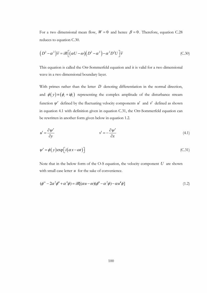
100

For a two dimensional mean flow, 0W = and hence 0β = . Therefore, equation C.28

reduces to equation C.30.

( ) ( )( )2 2 2 2 2 2D v iR U D D U vα α ω α α⎡ ⎤− = − − −⎣ ⎦ (C.30)

This equation is called the Orr-Sommerfeld equation and it is valid for a two dimensional

wave in a two dimensional boundary layer.

With primes rather than the letter D denoting differentiation in the normal direction,

and ( ) ( )r iy iφ φ φ≡ + representing the complex amplitude of the disturbance stream

function ψ ′ defined by the fluctuating velocity components u′ and v′ defined as shown

in equation 4.1 with definition given in equation C.31, the Orr-Sommerfeld equation can

be rewritten in another form given below in equation 1.2.

uyψ ′∂′ =∂

vxψ ′∂′ = −∂

(4.1)

( ) ( )expy i x tψ φ α ω′ = −⎡ ⎤⎣ ⎦ (C.31)

Note that in the below form of the O-S equation, the velocity component U are shown

with small case letter u for the sake of convenience.

2 4 2( 2 ) [( )( ) ]iv iR u uφ α φ α φ α ω φ α φ α φ′′ ′′ ′′− + = − − − (1.2)

101

A P P E N D I X D

DESCRIPTION OF THE COMPUTER PROGRAM

In order to conduct this study, a computer program written before in reference [1] has

been utilized. The Smith-van Ingen en procedure is implemented through another one

whish has been written in Fortan 77 programming language. The theory and procedure is

thoroughly explained in the above chapters 2, 3, 4 and 5. In order to prepare the inputs

for the en code, the original interactive boundary layer code is altered so that it now prints

out the boundary layer grid information which is used by the en code.

The program suite which is used in this study consists of three program codes, from

which two are essentially the same except for the input and output files are different to

examine upper and lower surfaces of the airfoil in consideration. The first program

written originally by Dr. Serkan Özgen during his Master of Science studies in 1994 is the

interactive boundary layer code with wake effects included is called the IBLW. In order to

solve for the stability equations and to employ the en procedure, a stability transition code

is written which originally inputs a single velocity profile and solves for the Falkner-Skan

profiles which are used to prove the feasibility of the procedure. The other two are altered

versions of the stability transition code called as ENLO and ENUP, where the only

difference between the two are the input and output files as mentioned above. These

altered versions read the velocity profiles stored at each boundary layer grid station which

are prepared by the IBLW code. The EN code can either be used to solve for the neutral

stability curve, or to predict transition.

In order to analyze an airfoil at any given angle of attack, user runs the IBLW code with

laminar region as long as feasible, and then runs the ENLO and ENUP code for the

upper and lower surfaces of the airfoil separating from the stagnation point which is also

calculated by the IBLW program extending through the trailing edge. The codes ENLO

and ENUP provide the user the physical frequencies, and the amplification rates related to

these frequencies. Depending on the user’s choice, at a value where the original instability

is amplified by a factor between e8 to e10, the transition location is determined and fed

back into the IBLW code as an external input. The actual solution is then obtained.

102

Note that as the compressibility effects are neglected, the solutions are valid only within

the incompressible range typically where the Mach number is less than 0.3. Therefore the

solution is limited to low to moderate Reynolds numbers. Also the Smith-van Ingen en

procedure is feasible for low to moderate angles-of-attack. For high values, laminar

separation point must be used as the transition mechanism for flows with adverse

pressure gradient.

The EN code has a MAIN routine and four subroutines which are briefly described

below.

In MAIN routine, the number of stations, their values, and the initial station for starting

the calculations are inputted. Also the user selects whether neutral stability curve or

transition is required. If transition is required, number of lines to be followed is entered.

This is done by giving a value for the mode flag as 0 for neutral stability of any integer less

than or equal to 20 for transition prediction. Also the non-dimensional station

coordinates; distances along the surface starting from the stagnation point and the

external velocity distribution at each station are input. With the additional information

about the chord Reynolds number, the stability Reynolds number for each station is

computed. One other input parameter is the initial guesses for eigenvalues α and ω to

be used at initiation. One may find good estimates from the Falkner-Skan solutions after

determining the pressure gradient.

The velocity profiles u and u′′ at stations are read by the subroutine PROFILE, the

neutral stability calculations are done by subroutine NEWTON, where the amplification

rated are calculated by the subroutine AMPL.

The subroutine OS is used to solve for the Orr-Sommerfeld equation, and includes the

block elimination algorithm described above. In the NEWTON subroutine, the

eigenvalue procedure explained is done. After convergence is achieved, physical

frequencies are computed. The AMPL subroutine is used for calculating the amplification

factor which is the key value in determining the onset of transition. After the code is run,

the amplification factors are printed at all stations, where the user is responsible to curve-

fit the data and to probe the location where the amplification rate has reached the value

desired to set the transition point.