Proceedings of ASME-JSME-KSME Joint Fluids Engineering Conference 2011 AJK2011-FED

July 24-29, 2011, Hamamatsu, Shizuoka, JAPAN

AJK2011-03023 MODELLING MULTIPHASE JET FLOWS FOR HIGH VELOCITY EMULSIFICATION

Mr David Ryan School of Chemical Engineering

University of Birmingham Birmingham, UK

Dr Mark Simmons School of Chemical Engineering

University of Birmingham Birmingham, UK

Dr Mike Baker Unilever Research &

Development Port Sunlight, Merseyside, UK

ABSTRACT Single phase steady-state Computational Fluid Dynamics

(CFD) simulations are presented for turbulent flow inside a

Sonolator (an industrial static mixer). Methodology is given

for obtaining high quality, converged, mesh-independent

results. Pressures, velocities and local specific turbulent

energy dissipation rates throughout the fluid domain are

obtained for three industrially-relevant mass flow rates at a

fixed nozzle orifice size. Discharge coefficients calculated at

the orifice are compared to literature values and to pilot plant

experiments for initial validation. Streamlines in the flow are

used to illustrate the presence of recirculation zones after the

nozzle. Thus, residence time and peak local specific turbulent

energy dissipation rates are calculated from streamline data as a

function of inlet position. Values of local specific turbulent

energy dissipation rate obtained are used to infer drop sizes for

emulsification of a multiphase mixture under dilute,

homogeneous flow conditions. The results show that different

drop size distributions may be produced depending on the inlet

condition of the multiphase mixture.

INTRODUCTION The Sonolator (Figure 1, Figure 2) is a static high shear

mixer used by industry to emulsify multiphase liquids by

forcing them at high pressure through a nozzle with a small

cats-eye shaped orifice. The high velocity jet formed impinges

on a fixed blade which splits the flow and is thought to cause

cavitation. A backpressure valve downstream maintains the

pressure in the main chamber. High local specific turbulent

energy dissipation rate ε (W∙kg-1

) is encountered which breaks

down larger dispersed phase droplets into smaller ones. The

physical mechanisms by which ε is generated are not currently

known.

Since these devices are used by industry, there is a need to

identify the precise mechanisms and locations of droplet

breakage and emulsification in different flow regimes, enabling

predictions of performance to be made. Mechanisms of

emulsification may include turbulent mixing, shear forces,

elongation or cavitation. Techniques for investigating the first

three of these mechanisms using single phase CFD are the

focus of this paper. The last mechanism, cavitation, is not

considered.

Previous literature results for the Sonolator or for liquid

whistles include: usage to disinfect wastewater in conjunction

with ozone [1], usage to remove unwanted dissolved gas from a

liquid [2] and investigations into the cavitation noise and its

interpretation [3]; however none of these works include any

flow analysis or application to emulsions. It is therefore

necessary to carry out research into the flow fields within the

Sonolator so that these processes could be better understood.

This paper presents the results of single phase steady-state

CFD simulations of the flow field inside the Sonolator. The

data is used to predict the likely maximum drop size obtained

when performing emulsification in such a device, assuming that

this occurs under dilute (< 1% by volume dispersed phase),

homogeneous flow (zero slip velocity) conditions [4]. Thus the

dispersed phase may be assumed to faithfully follow the

continuous phase flow field without affecting its properties.

Water was the working fluid and three mass flow rates of 0.033,

0.067 and 0.100 kg∙s-1

(2, 4 and 6 kg∙min-1

), were simulated

with a fixed Sonolator geometry, (nozzle orifice area

3.871 mm2 [0.0060 in

2]), using the Shear Stress Transport

(SST) turbulence model.

Basic validation is performed against pilot plant data, using

the discharge coefficient. Streamlines are introduced, from

them quantities at the inlet are derived which can be used for

multiphase analysis. The industrial application of this analysis

is discussed..

MODELLING THE SONOLATOR STATIC MIXER Figure 1 shows the main features of the Sonolator: a nozzle

with a narrow orifice, a turbulent jet from the liquid forced

through the orifice, the jet impinging on a fixed blade in the

main chamber, and the liquid travelling though the rest of the

device, past a back-pressure valve (not shown) and out of the

outlet.

The flow conditions and emulsification effect of the

Sonolator depend greatly on the exact cross-sectional area of

the orifice. The CFD carried out below is for a fixed area of

3.8710 mm2 (0.0060 in

2), unless stated otherwise. This area

represents a typical industrial nozzle.

FIGURE 1. DIAGRAM OF SONOLATOR DEVICE

CFD simulations The programs used to carry out the CFD simulations were

ANSYS ICEM for geometry creation and meshing, ANSYS

CFX-Pre for simulation set-up and ANSYS CFX-Solver for

running the simulations. Post-processing was carried out in

ANSYS CFD-Post and Microsoft Excel 2007.

Creating the Geometry in ANSYS ICEM The Sonolator 3D geometry dimensions were obtained

from scale drawings from Sonic Corp, Inc (US) and from

photographs of the nozzle, orifice, main chamber and blade of a

dismantled Sonolator taken at a pilot plant facility at Unilever

Research and Development, Port Sunlight, UK.

The 3D geometry shown in Figure 2 was constructed in

ANSYS ICEM by hand from the dimensions given.

Furthermore, all sharp corners in the fluid domain (angles

greater than 30°) were rounded off. This was to enable good

quality meshes and good convergence of the simulations. In

regions of high interest, such as the nozzle orifice, rounding

was still carried out but with a very tight radius of curvature.

The implications of the rounding of corners upon the results are

discussed later.

FIGURE 2. 3D WHOLE SONOLATOR GEOMETRY

The Sonolator was 165.1 mm in length along its axis. The

inlet diameter was 22.1 mm.

This paper presents simulation results generated using the

0.0060 in2 orifice geometry, see Figure 4. Industrial orifice

sizes range from 0.001 to 0.01 in2, thus the size used is within

this range.

The backpressure valve was omitted from the geometry,

since previous simulations had shown that local specific

turbulent energy dissipation rate at the valve was 1 or 2 orders

of magnitude lower than at either the orifice or the blade. This

meant that, in the following analysis, the presence of the valve

could not affect maximum droplet size predictions given.

Omitting the valve from the CFD geometry meant that the

geometry was a long narrow tube between the blade and the

outlet, as shown in Fig. 3.

FIGURE 3. 3D QUARTER SONOLATOR GEOMETRY FROM

TWO ANGLES

FIGURE 4. NOZZLE ORIFICE IN QUARTER MODEL

The Sonolator without its orifice and blade possesses

cylindrical symmetry. The orifice and blade break this

symmetry but instead create rectangular symmetry with two

symmetry planes: one vertical and one horizontal, see Figure 2.

These symmetries were used to model only one quarter of the

Sonolator instead of the whole flow domain, with consequent

75% saving in computational resources, see Figure 3. A closer

view of the orifice geometry in the quarter model is shown in

Figure 4. The physical and mathematical appropriateness of

this simplification is discussed later.

Creating the Mesh in ANSYS ICEM The mesh was created in ANSYS ICEM in three stages:

surface mesh, volume mesh, then prism mesh for each complete

mesh. Furthermore, each geometry had three meshes of

different resolutions created by this method. This was done to

demonstrate mesh independence in the simulation results.

The triangular surface mesh shown in Figure 5 was created

using patch independent triangular meshing, with increased

detail in regions of high curvature of the surface. Detail varied

from 3 mm maximum element size on flat surfaces to around

0.0625 mm on highly curved surfaces. This compared to an

inlet diameter of 22.1 mm, and a total geometry length of

165 mm. The maximum element size was 3.00 mm, 2.00 mm

and 1.75 mm for the three different size meshes for each

geometry.

FIGURE 5. SURFACE MESH FOR QUARTER MODEL

SHOWING TWO SYMMETRY PLANES

The tetrahedral volume mesh was created using the

Delaunay method from the existing surface mesh.

To ensure good wall treatment, a single-layer triangular

prism mesh was extruded into the volume mesh interior from

the surface mesh. ICEM then automated the merging of the

tetrahedral and prism meshes.

The local height of the single layer prism mesh was 1.5 of

a mesh element. This single layer was then split into 8, 12 or 15

layers according to which of the three overall mesh resolution

was needed. The height ratio between successive layers

was 1.4, this ensured many nodes were available close to the

wall for good wall treatment. This is visible in Figure 6 and

Figure 7.

FIGURE 6. CUTPLANE SHOWING TETRAHEDRAL AND

PRISM VOLUME ELEMENTS

FIGURE 7. CUTPLANE ON HIGHER RESOLUTION MESH

After each mesh generation step the intermediate mesh was

smoothed to, if possible, a quality statistic of 0.4 or above as

measured in ICEM. For the meshes used in these results

virtually all mesh elements in the final smoothed meshes had

quality about 0.4, with only a few isolated elements below this

cutoff.

The final smoothing step carried out on prism and

tetrahedral layers simultaneously had a slight decrease in prism

quality, but much greater compensating increase in tetrahedra

quality, rendering a much higher quality mesh overall.

The number of nodes in the simulations used for this paper

was between 48,000 and 200,000. Note that in CFX elements

define the mesh, however nodes are taken at vertices where the

volume elements join. Thus a typical 200,000 element mesh,

with 180,000 volume elements, only 70,000 nodes may exist.

Each simulation for each geometry or set of flow

conditions was carried out on three or four separate meshes of

different resolutions. This established mesh independence.

Results were then quoted from the highest resolution mesh.

Statistics such as pressure drop were read from the average of

the two highest resolution meshes, and error bars given as the

sample standard deviation of these two. The lowest resolution

mesh results were not used except as an extra check for mesh

independence. The average size of meshes 1, 2 and 3 were

respectively 80,000, 150,000 and 170,000 nodes.

Tetrahedral and prism meshing were used throughout. It

was not found possible to form a hexahedral (cubic) mesh of

sufficient mesh quality to run the simulation. This was probably

due to the many sharp internal 30º angles in the geometry

which did not lend themselves to being meshed with 90º-angled

cubes. Although it may have been possible to segment the

geometry, mesh different segments with tetra- or hexa-

elements and use generalised grid interfaces (GGI) to link

segments, earlier simulations found no advantage of using this

method over pure tetra-meshes, and extra overheads due to the

computationally intensive nature of GGI.

The symmetry plane geometries in ICEM were flat. The

surface mesh on each plane was checked to ensure that all mesh

elements were exactly in the geometric plane. All nodes which

deviated slightly from the plane, due to rounding errors while

smoothing the mesh, were moved back in the exact plane. The

maximum distance moved was 0.002 mm. This did not affect

the mesh quality appreciably.

Up to this point all work was carried out in ANSYS ICEM.

Once a mesh of suitable quality was obtained, it was exported

from ICEM in “Fluent v6” format for use in ANSYS CFX-Pre.

Simulation Setup in ANSYS CFX-Pre CFX-Pre was used to set up a simulation. Five main areas

had to be covered: simulation physics, symmetry conditions,

initial conditions, boundary conditions, simulation specific

options.

Simulation Physics. For the simulation physics the

following assumptions were made: single phase flow, water as

the fluid in the flow domain, incompressible flow, no heat

model or heat transfer, constant temperature 298.15 K (25°C),

constant density 997 kg∙m-3

, constant dynamic viscosity

8.684×10-4

Pa∙s (Tab. 1).

Flow fields in emulsions with oil phase less than 1 percent

by volume were considered similar enough to flow fields with

pure water to justify the single phase model to help investigate

multiphase flow. Furthermore, due to the low viscosity of

water, heating would be negligible. No heat model meant that

fluid properties such as density and viscosity could be treated

as constant.

Turbulence was modelled by the SST turbulence model.

This was chosen because it combined the good wall treatment

of the k-ω model with the good free stream behaviour of the k-ε

model. For the kind of conditions present in the Sonolator –

complex flows with severe pressure gradients, boundary layer

separation, strong streamline curvature – it overcame some

limitations of both k-ω and k-ε turbulence models [5-6]. In

addition, automatic wall treatment was used so that the

software would include a wall function wherever appropriate to

make the boundary flows physically realistic.

Steady state was felt justified since the turbulence model

eliminated the need to model individual turbulent eddies, and

provided parameters in steady state to approximate unsteady

variations in effective viscosity from turbulent eddy dissipation.

CFX would therefore model the Navier Stokes equations

with these physical assumptions.

Symmetry Conditions. Symmetry conditions were

imposed. The whole Sonolator geometry would have had

rectangular symmetry if it was modelled in totality. The

simplified quarter model for the Sonolator geometry, and the

resulting mesh which was actually used, therefore were

bounded by two extra symmetry plane conditions. The effect of

a symmetry plane was to force any velocity vector on the plane

to point within the same plane. (Velocity vectors on the central

axis where the two symmetry planes met were therefore were

doubly constrained, and could only point up or down the axis.)

The reasoning why it was felt valid to use symmetry to

simplify the geometry in this way was as follows. The steady

state solution obtained would represent a time averaged

solution. Although temporal oscillations in the flow fields

would temporarily break spatial rectangular symmetry; by time-

averaging, the symmetry of the geometric flow domain should

result in regained symmetry in the time-averaged flow solution.

Exceptions to this do occur: the Coanda effect [7] for example

causes a jet of fluid to cling to a nearby wall. In the case of the

Sonolator, the thin jet exits in the middle of a cylindrical

chamber, well away from the wall. So the Coanda effect would

not be likely to cause symmetry breaking in this case. In fact,

inside the Sonolator the jet was incident on a fixed blade which

it would cling to, both above and below, and in this way retain

the rectangular symmetry, not destroy it, by the Coanda effect.

Initial Conditions. Initial conditions would normally be

considered in a fully transient simulation. However, since these

simulations were steady state, initial conditions were not

needed.

Boundary Conditions. Boundary conditions came in

three varieties: wall, outlet and inlet.

The walls were smooth, no slip, stationary walls. All metal

surfaces in the real Sonolator device, including the inlet tube,

nozzle and orifice, main chamber, blade and outlet tubing, were

modelled with this wall condition. Future research may cover

small oscillations in the wall conditions, e.g. any small

oscillations the fixed blade may undergo.

The outlet was modelled in CFX as an “Opening”, with

absolute pressure 101,325 Pa (1 atm). This level could be set

freely without changing the simulation results, since cavitation

was not modelled. Mass, momentum and turbulence fields were

conserved at this boundary.

At the inlet a mass flow condition of 8.333×10-3

kg∙s-1

,

1.667×10-2

kg∙s-1

or 2.500×10-2

kg∙s-1

was set on the quarter

model. These correspond to flows of 2 kg∙min-1

, 4 kg∙min-1

,

6 kg∙min-1

on the whole model. Each of these three flow rates

was used in industry, and could be used to validate the CFD

work with pilot plant data. This mass flow condition was

equivalent to a fixed volumetric flow, and also equivalent to a

uniform velocity across the whole of the inlet tube.

Turbulence input at the inlet was kept at “Medium

(Intensity = 5%)” according to ANSYS’s recommendation in

the CFX-Pre help documentation for situations where the

incoming turbulence is unknown or not specified [8].

Simulation Specific Options. Some general simulation

specific parameters needed to be set for the simulation runs.

The simulation was run with a “physical timescale” of

0.01 s, the exact level did not affect the final results, but would

affect the speed at which they converged. For this system,

0.01 s was found optimal.

Each simulation was run for between 100 and 500

iterations until it had converged suitably. Convergence was

judged by ensuring the RMS residuals for momentum and mass

were below 10-5

, and that relevant monitor points, such as

average orifice velocity and pressure drop across the Sonolator,

had ceased to oscillate but each converged to a single value to 3

significant figures. Every result presented in this paper was

proved to be mesh independent by obtaining the same values

within suitable error bars from at least 3 different resolution

meshes.

A conservation target of 0.1% across the whole flow

domain was also set, ensuring that mass and momentum

conservation across the domain would not deviate by more than

1 part in 1,000. Comparisons of mass flow at the inlet with

those at the nozzle orifice verified this.

When the CFX-Pre simulation definition was finished it

was saved to a definition file for running in CFX-Solver.

Running the Simulation in ANSYS CFX-Solver For each different simulation, a run was set up in CFX-

Solver from the definition file exported from CFX-Pre. The

simulation could be iteratively converged from a flow field

which was zero everywhere. However to aid swifter

convergence the converged results of a relevant previous

simulation were normally used to initialize a later simulation.

Double precision arithmetic was selected. Although it

required more memory, it allowed RMS residuals to converge

to potentially 10-10

, instead of not converging below 10-4

in

single precision in some cases.

The results shown in this paper were run on a single Intel

Core 2 Duo processor. RMS residuals and user monitor points

were viewed, to judge convergence. When the simulation was

judged to have adequately converged it was stopped. Values

such as pressure drop across the Sonolator were noted from

relevant monitor points.

ANSYS CFD-Post was used to post-process the results

which are discussed below.

RESULTS AND DISCUSSION

TABLE 1. CONSTANT VALUES IN CFD EXPERIMENTS

Velocities and Pressures inside the Sonolator The parameters taken as constant in the simulations are

shown in Table 1. Two critical variables are the pressure drop

across the Sonolator, and orifice velocity. These are shown in

Table 2 for three different flow rates, and illustrated in Figure 8

and Figure 9 respectively. These two logarithmic plots are

both straight lines with slopes of two and unity respectively,

demonstrating that pressure drop was proportional to flow rate

squared (Figure 8), and velocity at orifice was proportional to

flow rate (Figure 9), in line with fundamental fluid dynamics

theory and dimensional analysis.

The error levels given in Table 2 represent the level of

mesh independence found within CFD, not a confidence that a

physical experiment would duplicate the result to within that

range.

TABLE 2. CFD PREDICTIONS OF FLOW PRESSURES AND

VELOCITIES

TABLE 3. REYNOLDS NUMBERS AND CFD PREDICTIONS

OF DISCHARGE COEFFICIENTS

FIGURE 8. PRESSURE DROP ACROSS SONOLATOR VS

FLOW RATE

FIGURE 9. VELOCITY AT NOZZLE ORIFICE VS FLOW RATE

Reynolds numbers and discharge coefficients were

calculated from the orifice velocity and device pressure drop.

The formulae used for Reynolds number is shown in Eq. (1),

and that for discharge coefficient [9] is shown in Eq. (2); the

values are shown in Table 3. (Note that to simplify the

discharge coefficient formula it has been assumed that “cross-

sectional area of orifice” divided by “cross-sectional area of

surrounding tube” is negligible.)

The discharge coefficients obtained from CFD were ≈ 0.75

(Table 3), which are approximately 15% higher than values

obtained from pilot plant studies carried out by the author,

which gave values of ≈ 0.65. These studies were carried out on

a Sonolator unit at the pilot plant at Unilever Research &

Development, Port Sunlight, UK. (This pilot plant data is

expected to be published in a future paper.)

Nevertheless, the CFD values compare favourably with

literature values for discharge coefficient for an orifice plate of

between 0.4 and 0.8 [9].

Therefore, the comparisons show that the CFD results were

of the right order of magnitude, and furthermore, CFD results

were within a tolerable margin of existing experimental data.

Reasons to explain the remaining 15% discrepancy

between CFD and pilot plant values for the discharge

coefficient include:

The orifice area value given by the manufacturer could

have been inaccurate given wear on the device and also

that the orifice edge sharpness in CFD and in the pilot

plant Sonolator was almost certainly different, a factor

which has a large effect on discharge coefficient [9].

The SST turbulence model, which assumes isotropic

turbulence, may not have complete accuracy when applied

to the flattened anisotropic turbulent jet present in the

Sonolator.

Flow Visualisation CFD illustrations are now given for various flow properties

in the Sonolator. The single flow chosen to illustrate these

properties is the medium mass flow rate of 0.0167 kg∙s-1

quarter

inlet (4 kg∙min-1

whole inlet), on the highest resolution mesh.

Values for y+ on the wall. Figure 10 shows a contour

plot of y+ (dimensionless wall distance) on the walls for the

medium flow rate. The peak y+ values were obtained on each

mesh with the highest flow rate; y+ peaks of 1.92 for the

highest resolution mesh and 5.25 for the medium resolution

mesh were obtained. Since the SST turbulence model used had

“Automatic” wall treatment, a wall function was introduced by

the software wherever necessary, and for either high or low y+

values the wall treatment would be suitable [10].

FIGURE 10. Y-PLUS VALUE CONTOUR PLOT ON WALLS

Velocity, pressure and turbulence. Figure 11 shows

the velocity field along the vertical symmetry plane with Fig.

12 providing a zoomed in view near to the nozzle and blade.

Figure 13 shows flow along the horizontal symmetry plane.

Axial velocity in Figure 11, Figure 12 and Figure 13 showed

flow moving from left (inlet) to right (outlet). The overall value

of axial velocity was positive, as expected for mass flow

downstream, however negative axial velocity (blue colour)

above the blade and nozzle represented material travelling

backwards in a recirculation zone (Figure 11, Figure 12). A fast

flattened jet (coloured red) was found exiting the nozzle orifice

and passing over the blade (Figure 11, Figure 12 and Figure

13). Note that the colour scheme is from -4 m∙s-1

to 4 m∙s-1

: any

velocities lower/higher than these are coloured completely blue

or red respectively. The peak velocity obtained in the middle of

the jet at the highest flow rate (6 kg∙min-1

whole inlet) was

36.4 m∙s-1

.

FIGURE 11. AXIAL VELOCITY ON VERTICAL SYMMETRY

PLANE OVER WHOLE SONOLATOR

FIGURE 12. AXIAL VELOCITY ON VERTICAL SYMMETRY

PLANE NEAR NOZZLE AND BLADE

FIGURE 13. AXIAL VELOCITY ON HORIZONTAL

SYMMETRY PLANE

Pressure drop from the inlet to the outlet of the Sonolator

at the highest flow rate was 591 kPa (5.91 bar), and at the

medium flow rate illustrated in Figure 14 was 265 kPa

(2.65 bar). One important feature was that almost all of the

pressure drop occurred across the nozzle orifice. The blade had

little effect on pressure drop.

Pressure drop over a volume of fluid is related to the

energy dissipated by turbulence, which is plotted as the local

specific turbulent energy dissipation rate, ε. After the sharp

pressure drop across the nozzle, turbulence is greatly increased,

as shown in Figure 15 in the turbulent jet directly after the

nozzle. Medium levels of turbulence remain in the recirculation

zone above the blade, and gradually die down as the flow

continues down the device. A log colour-scale is used to reveal

this spatial evolution.

FIGURE 14. TOTAL PRESSURE (INCLUDING VELOCITY

CONTRIBUTION) ON VERTICAL SYMMETRY PLANE

FIGURE 15. LOCAL SPECIFIC ENERGY DISSIPATION

RATE, ε (LOG SCALE) ON VERTICAL SYMMETRY PLANE

3D Structure. To visualise the 3D structure of the

turbulent jet an isosurface was created to show all points in the

flow with velocity magnitude of 5 m∙s-1

(Figure 16). The colour

of the surface represents the axial velocity, with pure red

representing exact downstream travel. (The white reflections

are only to help visualise the 3D structure, and do not contain

flow information.) The structure of the jet is seen to be

flattening and widening as it moves away from the orifice and

towards the blade, and then forming a thick lobe above the

blade, which would be expected to repeat symmetrically in the

other three quarters of the flow.

FIGURE 16. ISOSURFACE OF VELOCITY MAGNITUDE

5 m∙s-1

, COLOURED BY AXIAL VELOCITY.

Streamlines were constructed which started at the inlet and

followed the flow throughout the whole flow domain. Three

different 3D angles are given in Figure 17. The streamlines

make recirculation zones much more visible than a plane

colouration.

A prominent vortex is revealed in the third view diagonally

above the turbulent jet. It is thought that the mass flow

downstream in the turbulent jet entrains the fluid above it, and

thus conservation of mass causes a recirculation to form in this

region.

The colour of the streamlines also reveal the 3D region in

the jet where ε is high, since the colour represents turbulent

dissipation of 1 to 10,000 W∙kg-1

on a log colour scale by blue

through to red. The saturated red streamline region thereby

represents ε above 10,000 W∙kg-1

.

FIGURE 17. STREAMLINES OF VELOCITY ORIGINATING

FROM WHOLE INLET FROM 3 DIFFERENT ANGLES

FIGURE 18. DIFFERENT BEHAVIOUR OF STREAMLINES

ORIGINATING FROM DIFFERENT INLET REGIONS

The flow structure revealed by the streamlines originating

from the inlet is complex. However, the streamlines originating

from some regions of the inlet do not have complex behaviour

associated with them. Figure 18 shows how one inlet region

gives rise to streamlines which go straight through the

Sonolator with no recirculation, whereas an different small inlet

region when transported downstream by the streamlines shows

chaotic recirculation. These differences between inlet regions,

as revealed by streamlines evolution downstream, will later be

used to characterise different regions of the inlet.

Each point on a streamline has flow properties such as

pressure, velocity and turbulence associated with it. By

considering that a small oil droplet introduced into an otherwise

aqueous flow will hardly affect the flow at all, but instead

follow the existing streamlines, it is possible to deduce results

about a low-concentration, homogeneous multiphase flow [4]

from the single phase flow data.

Streamline Analysis Therefore streamlines may be used to deduce multiphase

results. A streamline is a potential way for a multiphase droplet

to travel through the fluid, and at each point on the streamline

fluid properties such as ε exist which could cause measurable

changes in the dispersed phase droplet.

Pairs of properties existing on streamlines can be plotted

on a suitable x-y scatter graph. Moreover, streamlines from

different flow rates can be plotted on the same graph to enable

direct comparison of flow properties of the different flow rates.

Figure 19 shows axial velocity plotted against axial

distance, as experienced on various streamlines in the flow. The

three colours (green, blue, red) here represent the three mass

flow rates (2, 4 and 6 kg∙min-1

) investigated. The multiple lines

of the same colour represent the multiple streamlines for the

same flow rate originating from points evenly spread across the

inlet. The total space occupied by each colour graph represents

information about what flow properties exist for that flow rate.

By superimposing these three graphs, it is clearly visible that

they are self-similar by scaling the vertical axis appropriately.

This indicates that axial velocities are proportional to the flow

rate. A hypothesis would therefore be that velocity vectors

overall scale according to the flow rate, within the range of

Reynolds numbers investigated here.

Figure 20 plots ε against axial distance for the same three

sets of 24 streamlines. Again, the scaling relationship reveals

itself as a vertical shift in the graphs, supporting the hypothesis.

Closer inspection reveals an 8-fold (equivalent to (4/2)3-fold)

increase in ε when increasing flow rate from 2 to 4 kg∙min-1

,

and a (6/4)3-fold increase from 4 to 6 kg∙min

-1. This is evidence

for ε scaling according to the cube of the flow rate.

Dimensional analysis confirms that this is the correct

proportionality between ε and flow rate.

FIGURE 19. AXIAL VELOCITY VS AXIAL DISTANCE FOR 3

DIFFERENT FLOW RATES, EACH ILLUSTRATED ALONG 24 STREAMLINES

FIGURE 20. LOCAL SPECIFIC ENERGY DISSIPATION

RATE, ε (LOG SCALE) VS AXIAL DISTANCE.

Both Figure 19 and Figure 20 clearly show spatial

evolution of streamlines, and identify recirculation zones in

terms of loops traced on the respective graphs.

Figure 20 also reveals where the peaks in ε are situated, in

terms of axial position. The two biggest peaks are at z = 0 mm

and z = 6 mm. These correspond to the orifice and sharp front

edge of the blade.

Closer inspection, and some extra analysis, has shown that

for around 80% of streamlines the maximum value of ε is

located at the orifice, but for the remaining 20% of streamlines

a higher value of ε is experienced at the blade instead. These

are the only two high peaks given in the chart. Isosurfaces of ε

in CFD-Post show that the reason why less streamlines

experience peak ε at the blade edge is due to the smaller surface

area of the blade edge compared with the cross-sectional area

of the orifice.

Supposing that a small oil droplet travelled along such a

streamline, it would be expected that this maximum value of ε

would play a major role in determining the final droplet size

distribution from the oil droplet as it breaks.

Moreover, the orifice would be expected to determine

around 80% (by volume) of oil droplet sizes in a dilute

emulsion, compared to 20% at the blade.

Inlet Functions and Flow Zones For any incident oil droplet, the only factor which

determines the history of local specific turbulent energy

dissipation rate it undergoes is the position it starts at on the

inlet. Therefore, by tracing relevant flow variables backwards

from streamlines, or measuring their maximum across the

whole streamline, such derived variables can be plotted across

the whole inlet surface.

Relevant derived streamline variables are thought to

include the following: residence time on a streamline,

maximum value of ε experienced along a streamline. By

taking a balance between the dynamic pressure forces in a

turbulent flow acting to disrupt a droplet and the restorative

forces due to surface tension acting to stabilize it, Hinze [11]

developed a criterion for droplet breakage based upon a critical

Weber number, We, which is the ratio of these quantities

By relating the average kinetic energy per unit mass,

represented in Eq. (3) by u2, to the local specific turbulent

energy dissipation rate, ε, assuming homogeneous isotropic

turbulence, Hinze obtained [11]

This correlation allows maximum droplet diameter to be

calculated if the history of ε is known, albeit with the

limitations of the assumptions made of isotropic homogeneous

turbulence and a dilute dispersed phase with no drop

coalescence. Assuming a constant continuous phase density

of 997 kg∙m-3

and approximate interfacial tension of

10 mN∙m-1

, Eq. (4) can be simplified to Eq. (5) which gives a

typical maximum droplet diameter on each streamline from the

corresponding maximum value of ε:

where B = 7.2631×10-4

. Since Dmax is proportional to ε-0.4

, and

ε is proportional to Q3 and also to M

3 (volumetric and mass

flow rates cubed), therefore Dmax is proportional to Q-1.2

and to

M-1.2

. This scaling relation makes it possible to derive

maximum droplet sizes for different flow rates, based on the

data for the fixed flow rate of 0.01667 kg∙s-1

quarter inlet

(4 kg∙min-1

whole inlet)

The three derived functions; residence time on streamline,

maximum ε on streamline, maximum droplet size on

streamline; are now given for the fixed flow rate as 2D plots

across the whole inlet surface in Figure 21, Figure 22 and

Figure 23 respectively. Note that the data for the whole inlet

was found by using the symmetry conditions to reflect the data

on the quarter inlet twice.

(continued overleaf)

FIGURE 21. RESIDENCE TIME ACROSS WHOLE INLET

FIGURE 22. PEAK LOCAL SPECIFIC TURBULENT ENERGY

DISSIPATION RATES ACROSS WHOLE INLET

These three surface plots (Figure 21, Figure 22 and Figure

23) reveal information about what dispersed phase droplets

present in low concentration are likely to experience when

introduced into various inlet regions. These results could be

extrapolated to higher concentrations with the caveat that drop

coalescence and the need to treat the motion of drops as a

discrete phase from the continuum become increasingly

important as the concentration increases, with consequent

effects of the drops upon the continuum mean flow and

turbulence [e.g. 12].

To make interpretation clearer, the information in these

three charts is combined into a single chart, Figure 24, which

separates out the streamline experiences into 6 main zones.

FIGURE 23. TYPICAL MAXIMUM DROPLET DIAMETER VS

INLET POSITION

FIGURE 24. ZONING OF WHOLE INLET SURFACE BY

CHARACTERISTICS OF STREAMLINES ORIGINATING AT EACH LOCATION ON SURFACE

Table 4 gives the corresponding names and flow properties

in each zone. Of particular note is the fact that recirculating

streamlines are not found in zones E and F, and that comparable

values of ε between 30 kW∙kg-1

and 70 kW∙kg-1

are found

across streamlines from nearly the whole inlet surface, with the

exception of streamlines originating in zone B (Blade), which

experience values of an order of magnitude higher (circa

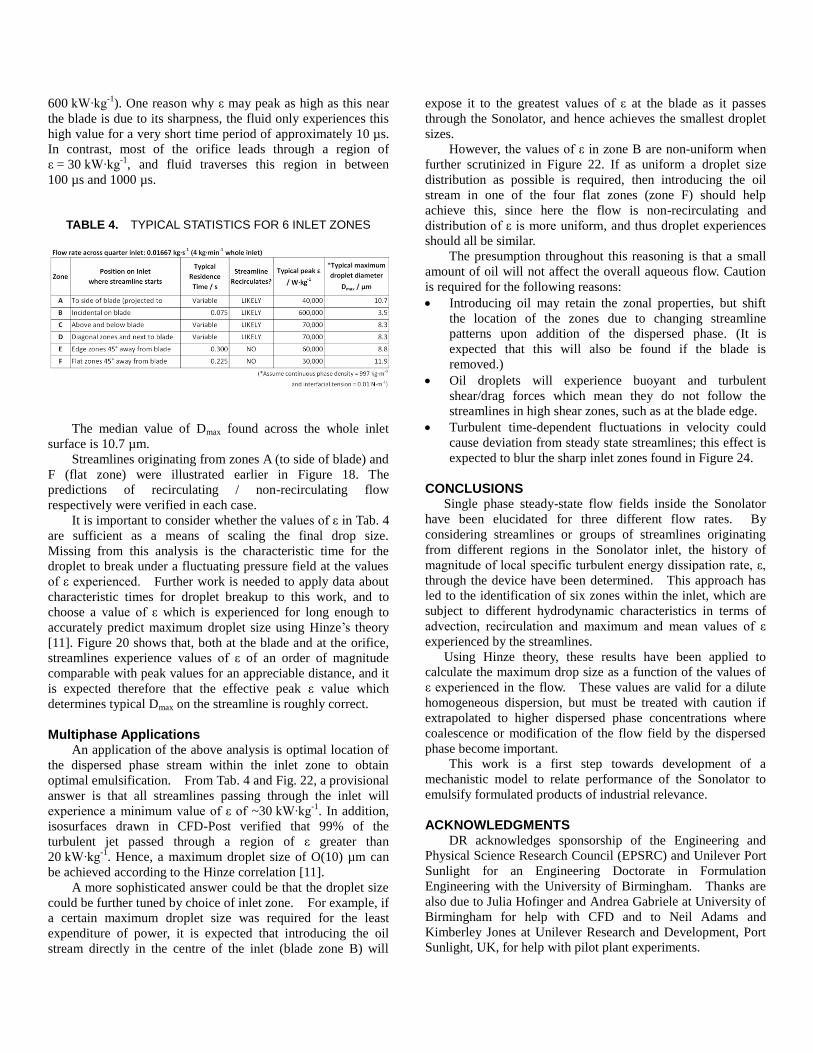
600 kW∙kg-1

). One reason why ε may peak as high as this near

the blade is due to its sharpness, the fluid only experiences this

high value for a very short time period of approximately 10 µs.

In contrast, most of the orifice leads through a region of

ε = 30 kW∙kg-1

, and fluid traverses this region in between

100 µs and 1000 µs.

TABLE 4. TYPICAL STATISTICS FOR 6 INLET ZONES

The median value of Dmax found across the whole inlet

surface is 10.7 µm.

Streamlines originating from zones A (to side of blade) and

F (flat zone) were illustrated earlier in Figure 18. The

predictions of recirculating / non-recirculating flow

respectively were verified in each case.

It is important to consider whether the values of ε in Tab. 4

are sufficient as a means of scaling the final drop size.

Missing from this analysis is the characteristic time for the

droplet to break under a fluctuating pressure field at the values

of ε experienced. Further work is needed to apply data about

characteristic times for droplet breakup to this work, and to

choose a value of ε which is experienced for long enough to

accurately predict maximum droplet size using Hinze’s theory

[11]. Figure 20 shows that, both at the blade and at the orifice,

streamlines experience values of ε of an order of magnitude

comparable with peak values for an appreciable distance, and it

is expected therefore that the effective peak ε value which

determines typical Dmax on the streamline is roughly correct.

Multiphase Applications An application of the above analysis is optimal location of

the dispersed phase stream within the inlet zone to obtain

optimal emulsification. From Tab. 4 and Fig. 22, a provisional

answer is that all streamlines passing through the inlet will

experience a minimum value of ε of ~30 kW∙kg-1

. In addition,

isosurfaces drawn in CFD-Post verified that 99% of the

turbulent jet passed through a region of ε greater than

20 kW∙kg-1

. Hence, a maximum droplet size of O(10) µm can

be achieved according to the Hinze correlation [11].

A more sophisticated answer could be that the droplet size

could be further tuned by choice of inlet zone. For example, if

a certain maximum droplet size was required for the least

expenditure of power, it is expected that introducing the oil

stream directly in the centre of the inlet (blade zone B) will

expose it to the greatest values of ε at the blade as it passes

through the Sonolator, and hence achieves the smallest droplet

sizes.

However, the values of ε in zone B are non-uniform when

further scrutinized in Figure 22. If as uniform a droplet size

distribution as possible is required, then introducing the oil

stream in one of the four flat zones (zone F) should help

achieve this, since here the flow is non-recirculating and

distribution of ε is more uniform, and thus droplet experiences

should all be similar.

The presumption throughout this reasoning is that a small

amount of oil will not affect the overall aqueous flow. Caution

is required for the following reasons:

Introducing oil may retain the zonal properties, but shift

the location of the zones due to changing streamline

patterns upon addition of the dispersed phase. (It is

expected that this will also be found if the blade is

removed.)

Oil droplets will experience buoyant and turbulent

shear/drag forces which mean they do not follow the

streamlines in high shear zones, such as at the blade edge.

Turbulent time-dependent fluctuations in velocity could

cause deviation from steady state streamlines; this effect is

expected to blur the sharp inlet zones found in Figure 24.

CONCLUSIONS Single phase steady-state flow fields inside the Sonolator

have been elucidated for three different flow rates. By

considering streamlines or groups of streamlines originating

from different regions in the Sonolator inlet, the history of

magnitude of local specific turbulent energy dissipation rate, ε,

through the device have been determined. This approach has

led to the identification of six zones within the inlet, which are

subject to different hydrodynamic characteristics in terms of

advection, recirculation and maximum and mean values of ε

experienced by the streamlines.

Using Hinze theory, these results have been applied to

calculate the maximum drop size as a function of the values of

ε experienced in the flow. These values are valid for a dilute

homogeneous dispersion, but must be treated with caution if

extrapolated to higher dispersed phase concentrations where

coalescence or modification of the flow field by the dispersed

phase become important.

This work is a first step towards development of a

mechanistic model to relate performance of the Sonolator to

emulsify formulated products of industrial relevance.

ACKNOWLEDGMENTS DR acknowledges sponsorship of the Engineering and

Physical Science Research Council (EPSRC) and Unilever Port

Sunlight for an Engineering Doctorate in Formulation

Engineering with the University of Birmingham. Thanks are

also due to Julia Hofinger and Andrea Gabriele at University of

Birmingham for help with CFD and to Neil Adams and

Kimberley Jones at Unilever Research and Development, Port

Sunlight, UK, for help with pilot plant experiments.

NOMENCLATURE AND ABBREVIATIONS ANSYS Software developers of the CFX package

A Nozzle Orifice Cross-sectional Area (m2)

B Constant (s3m

-1 )

CD Discharge Coefficient

CFD Computational Fluid Dynamics

CFX Implementation of CFD software by ANSYS

Dmax Maximum droplet diameter

DH Nozzle Orifice Hydraulic Diameter (m)

GGI Generalised Grid Interface: used to join two different

surface meshes in a plane separating

two different flow domains

k Turbulent kinetic energy

M Mass Flow Rate (whole) (kg∙s-1

)

P Pressure drop from inlet to outlet (Pa)

Q Volumetric Flow Rate (whole) (m3∙s

-1)

SST Shear Stress Transport turbulence model

Re Reynolds Number

T Ambient Temperature (K)

v Nozzle Orifice Average Velocity (m∙s-1

)

z Axial Position (m)

ε Local specific turbulent energy dissipation rate

(W∙kg-1

or m2s

-3)

ρ Water Density under ambient conditions (kg∙m-3

)

µ Dynamic viscosity of water under experimental

conditions (Pa∙s)

σ Interfacial tension (N∙m-1

)

ν Kinematic viscosity of water (m2∙s

-1)

ω Turbulent frequency (Hz)

REFERENCES [1] Chand, R., Bremner, D. H., Namkung, K. C., Collier, P. J.,

Gogate, P. R., 2007 “Water disinfection using the novel

approach of ozone and a liquid whistle reactor”.

Biochemical Engineering Journal, 35(3), August, pp. 357-

364

[2] Clark, A., Dewhurst. R. J., Payne, P. A., Ellwood, C., 2001

“Degassing a liquid stream using an ultrasonic whistle”

IEEE Ultrasonics Symposium Proceedings. eds. Yuhas, D.

E., Schneider, S. C., Vols 1 and 2 of Ultrasonics

Symposium, pp. 579-582

[3] Quan, K., Avvaru, B., Pandit, A. B., 2010 “Measurement

and interpretation of cavitation noise in a hybrid

hydrodynamic cavitating device” AlChE Journal. In Print.

[4] Wallis, G.B., 1969. One Dimensional Two-Phase Flow,

McGraw-Hill, New York.

[5] Menter, F. R., 1994 “Two-Equation Eddy-Viscosity

Turbulence Models for Engineering Applications,” AIAA

Journal, 32(8), pp. 1598-1605

[6] Bardina, J.E., Huang, P.G. and Coakley, T.J., 1997

“Turbulence Modeling Validation Testing and Development”

NASA Technical Memorandum 110446

[7] Tritton, D.J., 1977. “Physical Fluid Dynamics”, Van

Nostrand Reinhold. Section 22.7, The Coanda Effect

[8] “CFX-Pre Release Notes” ANSYS Inc, software CFX-Pre

v12.1, page “Inlet (subsonic), Mass and Momentum,

Turbulence”

[9] Perry, R. H., Green, D. W., eds., 1998. Perry’s Chemical

Engineers’ Handbook, 7th ed., McGraw-Hill, New York,

Chap. 8, p. 48, Chap. 10, p. 16.

[10] “CFX-Pre Release Notes” ANSYS Inc, software CFX-Pre

v12.1, page “ANSYS CFX-Solver Modeling Guide,

Turbulence and Near-Wall Modeling, Modeling Flow Near

the Wall”

[11] Hinze, J. O., 1955. “Fundamentals of the Hydrodynamic

Mechanism of Splitting in Dispersion Processes”. A.I.Ch.E.

Journal, 1(3), September, p. 295. [12] Simmons, M.J.H., Azzopardi, B.J., 2001. “Drop size

distributions in dispersed liquid-liquid pipe flow”, Int. J.

Multiphase Flow, 27(5), p. 843.