albert-lászló barabási network science communities · pdf...
TRANSCRIPT

ALBERT-LÁSZLÓ BARABÁSI
NETWORK SCIENCECOMMUNITIES
9
ACKNOWLEDGEMENTS MÁRTON PÓSFAI NICOLE SAMAYROBERTA SINATRA
SARAH MORRISONAMAL HUSSEINI
NORMCOREONCE UPON A TIME PEOPLE WERE BORN INTO COMMUNITIES AND HAD TO FIND THEIR INDIVIDUALITY. TODAY PEOPLE ARE BORN INDIVIDUALS AND HAVE TO FIND THEIR COMMUNITIES.
MASS INDIE RESPONDS TO THIS SITUATION BY CREATING CLIQUES OF PEOPLE IN THE KNOW, WHILE NORMCORE KNOWS THE REAL FEAT IS HARNESSING THE POTENTIAL FOR CONNECTION TO SPRING UP. IT'S ABOUT ADAPABILITY, NOT EXCLUSIVITY.
Introduction
Introduction
Basics of Communities
Hierarchical Clustering
Modularity
Overlapping Communities
Characterizing Communities
Testing Communities
Summary
Homework
ADVANCED TOPICS 9.A
Counting Partitions
ADVANCED TOPICS 9.B
Hiearchical Modularity
ADVANCED TOPICS 9.C
Modularity
ADVANCED TOPICS 9.D
Fast Algorithms for Community Detection
ADVANCED TOPICS 9.E
Threshold for clique percolation
Homework
Bibliography
1
2
3
4
5
6
7
8
9
INDEX
This book is licensed under aCreative Commons: CC BY-NC-SA 2.0.PDF V26, 05.09.2014
Figure 9.0 (cover image)
Art & Networks: K-Mode: Youth Mode
K-Mode is an art collective that publishes trend reports with an unusual take on various concepts. The image shows a page from Youth Mode: A Report on Freedom, discussing the subtle shift in the origins and the meaning of communities, the topic of this chapter [1].
10
11
12
13
14

INTRODUCTIONCOMMUNITIES 3
SECTION 9.1
Belgium appears to be the model bicultural society: 59% of its citizens are Flemish, speaking Dutch and 40% are Walloons who speak French. As multiethnic countries break up all over the world, we must ask: How did this country foster the peaceful coexistence of these two ethnic groups since 1830? Is Belgium a densely knitted society, where it does not matter if one is Flemish or Walloon? Or we have two nations within the same bor-ders, that learned to minimize contact with each other?
The answer was provided by Vincent Blondel and his students in 2007, who developed an algorithm to identify the country’s community struc-ture. They started from the mobile call network, placing individuals next to whom they regularly called on their mobile phone [2]. The algorithm revealed that Belgium’s social network is broken into two large clusters of communities and that individuals in one of these clusters rarely talk with individuals from the other cluster (Figure 9.1). The origin of this separation became obvious once they assigned to each node the language spoken by each individual, learning that one cluster consisted almost exclusively of French speakers and the other collected the Dutch speakers.
In network science we call a community a group of nodes that have a higher likelihood of connecting to each other than to nodes from other communities. To gain intuition about community organization, next we discuss two areas where communities play a particularly important role:
• Social NetworksSocial networks are full of easy to spot communities, something that scholars have noticed decades ago [3,4,5,6,7]. Indeed, the employees of a company are more likely to interact with their coworkers than with employees of other companies [3]. Consequently work places ap-pear as densely interconnected communities within the social net-work. Communities could also represent circles of friends, or a group of individuals who pursue the same hobby together, or individuals living in the same neighborhood.A social network that has received particular attention in the context
INTRODUCTION
Communities extracted from the call pattern of the consumers of the largest Belgian mo-bile phone company. The network has about two million mobile phone users. The nodes correspond to communities, the size of each node being proportional to the number of in-dividuals in the corresponding community. The color of each community on a red–green scale represents the language spoken in the particular community, red for French and green for Dutch. Only communities of more than 100 individuals are shown. The commu-nity that connects the two main clusters con-sists of several smaller communities with less obvious language separation, capturing the culturally mixed Brussels, the country’s cap-ital. After [2].
Figure 9.1Communities in Belgium
COMMUNITIES

INTRODUCTION4COMMUNITIES
of community detection is known as Zachary’s Karate Club (Figure 9.2) [7], capturing the links between 34 members of a karate club. Given the club's small size, each club member knew everyone else. To uncov-er the true relationships between club members, sociologist Wayne Zachary documented 78 pairwise links between members who regu-larly interacted outside the club (Figure 9.2a).
The interest in the dataset is driven by a singular event: A conflict be-tween the club’s president and the instructor split the club into two. About half of the members followed the instructor and the other half the president, a breakup that unveiled the ground truth, representing club's underlying community structure (Figure 9.2a). Today communi-ty finding algorithms are often tested based on their ability to infer these two communities from the structure of the network before the split.
• Biological NetworksCommunities play a particularly important role in our understand-ing of how specific biological functions are encoded in cellular net-works. Two years before receiving the Nobel Prize in Medicine, Lee Hartwell argued that biology must move beyond its focus on single genes. It must explore instead how groups of molecules form func-tional modules to carry out a specific cellular functions [10]. Ravasz and collaborators [11] made the first attempt to systematically iden-tify such modules in metabolic networks. They did so by building an algorithm to identify groups of molecules that form locally dense communities (Figure 9.3).
Communities play a particularly important role in understanding human diseases. Indeed, proteins that are involved in the same dis-ease tend to interact with each other [12,13]. This finding inspired the disease module hypothesis [14], stating that each disease can be linked to a well-defined neighborhood of the cellular network.
The examples discussed above illustrate the diverse motivations that drive community identification. The existence of communities is rooted in who connects to whom, hence they cannot be explained based on the de-gree distribution alone. To extract communities we must therefore inspect a network’s detailed wiring diagram. These examples inspire the starting hypothesis of this chapter:
H1: Fundamental Hypothesis
A network’s community structure is uniquely encoded in its wiring diagram.
According to the fundamental hypothesis there is a ground truth about a network’s community organization, that can be uncovered by inspecting Aij.
The purpose of this chapter is to introduce the concepts necessary to
(a) The connections between the 34 members of Zachary's Karate Club. Links capture in-teractions between the club members out-side the club. The circles and the squares denote the two fractions that emerged af-ter the club split in two. The colors capture the best community partition predicted by an algorithm that optimizes the modulari-ty coefficient M (SECTION 9.4). The commu-nity boundaries closely follow the split: The white and purple communities capture one fraction and the green-orange communi-ties the other. After [8].
(b) The citation history of the Zachary karate club paper [7] mirrors the history of com-munity detection in network science. In-deed, there was virtually no interest in Zachary’s paper until Girvan and Newman used it as a benchmark for community de-tection in 2002 [9]. Since then the number of citations to the paper exploded, reminis-cent of the citation explosion to Erdős and Rényi’s work following the discovery of scale-free networks (Figure 3.15).
The frequent use Zachary’s Karate Club network as a benchmark in community detection inspired the Zachary Karate Club Club, whose tongue-in-cheek statute states: “The first scientist at any conference on networks who uses Zachary's karate club as an example is inducted into the Zachary Karate Club Club, and awarded a prize.”
Hence the prize is not based on merit, but on the simple act of participation. Yet, its recipients are prominent network scien-tists (http://networkkarate.tumblr.com/). The figure shows the Zachary Karate Club trophy, which is always held by the latest inductee. Photo courtesy of Marián Boguñá.
Figure 9.2Zachary’s Karate Club
4
20
22
21 9
28
3
27
18
19
23
297
17
24
33
16
30 34
26
25
328
21
12
11
65
13
14
31
1015
908070605040302010
1980
CITATIONS
YEAR1985 1990 1995 2000 2005 2010 2015
(a)
(b)

INTRODUCTION5COMMUNITIES
understand and identify the community structure of a complex network. We will ask how to define communities, explore the various community characteristics and introduce a series of algorithms, relying on different principles, for community identification.
The E. coli metabolism offers a fertile ground to investigate the community structure of bi-ological systems [11].
(a) The biological modules (communities) iden-tified by the Ravasz algorithm [11] (SECTION 9.3). The color of each node, capturing the predominant biochemical class to which it belongs, indicates that different func-tional classes are segregated in distinct network neighborhoods. The highlighted region selects the nodes that belong to the pyrimidine metabolism, one of the predict-ed communities.
(b) The topologic overlap matrix of the E. coli metabolism and the corresponding den-drogram that allows us to identify the mod-ules shown in (a). The color of the branches reflect the predominant biochemical role of the participating molecules, like car-bohydrates (blue), nucleotide and nucleic acid metabolism (red), and lipid metabo-lism (cyan).
(c) The red right branch of the dendrogram tree shown in (b), highlighting the region corresponding to the pyridine module.
(d) The detailed metabolic reactions within the pyrimidine module. The boxes around the reactions highlight the communities pre-dicted by the Ravasz algorithm.
After [11].
Figure 9.3Communities in Metabolic Networks
(a)
(c)
(d)
(b)

BASICS OF COMMUNITIESCOMMUNITIES 6
SECTION 9.2
What do we really mean by a community? How many communities are in a network? How many different ways can we partition a network into communities? In this section we address these frequently emerging ques-tions in community identification.
DEFINING COMMUNITIESOur sense of communities rests on a second hypothesis (Figure 9.4):
H2: Connectedness and Density Hypothesis
A community is a locally dense connected subgraph in a network.
In other words, all members of a community must be reached through oth-er members of the same community (connectedness). At the same time we expect that nodes that belong to a community have a higher probability to link to the other members of that community than to nodes that do not belong to the same community (density). While this hypothesis consider-ably narrows what would be considered a community, it does not uniquely define it. Indeed, as we discuss below, several community definitions are consistent with H2.
Maximum CliquesOne of the first papers on community structure, published in 1949, de-
fined a community as group of individuals whose members all know each other [5]. In graph theoretic terms this means that a community is a com-plete subgraph, or a clique. A clique automatically satisfies H2: it is a con-nected subgraph with maximal link density. Yet, viewing communities as cliques has several drawbacks:
• While triangles are frequent in networks, larger cliques are rare.
• Requiring a community to be a complete subgraph may be too re-strictive, missing many other legitimate communities. For example, none of the communities of Figure 9.2 and 9.3 correspond to complete subgraphs.
BASICS OF COMMUNITIES
Communities are locally dense connected subgraphs in a network. This expectation re-lies on two distinct hypotheses:
Connectedness HypothesisEach community corresponds to a connected subgraph, like the subgraphs formed by the orange, green or the purple nodes. Conse-quently, if a network consists of two isolated components, each community is limited to only one component. The hypothesis also im-plies that on the same component a commu-nity cannot consist of two subgraphs that do not have a link to each other. Consequently, the orange and the green nodes form separate communities.
Density HypothesisNodes in a community are more likely to con-nect to other members of the same commu-nity than to nodes in other communities. The orange, the green and the purple nodes satisfy this expectation.
Figure 9.4Connectedness and Density Hypothesis

BASICS OF COMMUNITIES7COMMUNITIES
(a) CliquesA clique corresponds to a complete sub-graph. The highest order clique of this net-work is a square, shown in orange. There are several three-node cliques on this network. Can you find them?
(b) Strong CommunitiesA strong community, defined in (9.1), is a connected subgraph whose nodes have more links to other nodes in the same com-munity that to nodes that belong to other communities. Such a strong community is shown in purple. There are additional strong communities on the graph - can you find at least two more?
(c) Weak CommunitiesA weak community defined in (9.2) is a sub-graph whose nodes’ total internal degree exceeds their total external degree. The green nodes represent one of the several possible weak communities of this network.
Figure 9.5Defining Communities
(a)
(b)
(c)
Strong and Weak CommunitiesTo relax the rigidity of cliques, consider a connected subgraph C of NC
nodes in a network. The internal degree kiint of node i is the number of links
that connect i to other nodes in C. The external degree kiext is the number of
links that connect i to the rest of the network. If kiext=0, each neighbor of
i is within C, hence C is a good community for node i. If kiint=0, then node i
should be assigned to a different community. These definitions allow us to distinguish two kinds of communities (Figure 9.5):
• Strong CommunityC is a strong community if each node within C has more links within the community than with the rest of the graph [15,16]. Specifically, a subgraph C forms a strong community if for each node i ∈ C,
. (9.1)
• Weak CommunityC is a weak community if the total internal degree of a subgraph ex-ceeds its total external degree [16]. Specifically, a subgraph C forms a weak community if
. (9.2)
A weak community relaxes the strong community requirement by al-lowing some nodes to violate (9.1). In other words, the inequality (9.2) ap-plies to the community as a whole rather than to each node individually.
Note that each clique is a strong community, and each strong commu-nity is a weak community. The converse is generally not true (Figure 9.5).
The community definitions discussed above (cliques, strong and weak communities) refine our notions of communities. At the same time they indicate that we do have some freedom in defining communities.
NUMBER OF COMMUNITIESHow many ways can we group the nodes of a network into commu-
nities? To answer this question consider the simplest community find-ing problem, called graph bisection: We aim to divide a network into two non-overlapping subgraphs, such that the number of links between the nodes in the two groups, called the cut size, is minimized (BOX 9.1).
Graph PartitioningWe can solve the graph bisection problem by inspecting all possible di-
visions into two groups and choosing the one with the smallest cut size. To determine the computational cost of this brute force approach we note that the number of distinct ways we can partition a network of N nodes into groups of N1 and N2 nodes is
. (9.3)
k inti (C ) > kext
i (C )
∑i∈C
k inti (C ) > ∑
i∈Ckext
i (C )
N!N1!N2!
BASICS OF COMMUNITIES8COMMUNITIES
BOX 9.1GRAPH PARTITIONING
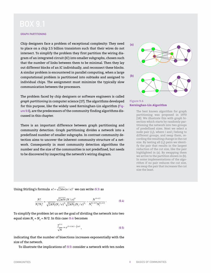
Chip designers face a problem of exceptional complexity: They need to place on a chip 2.5 billion transistors such that their wires do not intersect. To simplify the problem they first partition the wiring dia-gram of an integrated circuit (IC) into smaller subgraphs, chosen such that the number of links between them to be minimal. Then they lay out different blocks of an IC individually, and reconnect these blocks. A similar problem is encountered in parallel computing, when a large computational problem is partitioned into subtasks and assigned to individual chips. The assignment must minimize the typically slow communication between the processors.
The problem faced by chip designers or software engineers is called graph partitioning in computer science [17]. The algorithms developed for this purpose, like the widely used Kerninghan-Lin algorithm (Fig-
ure 9.6), are the predecessors of the community finding algorithms dis-cussed in this chapter.
There is an important difference between graph partitioning and community detection: Graph partitioning divides a network into a predefined number of smaller subgraphs. In contrast community de-tection aims to uncover the inherent community structure of a net-work. Consequently in most community detection algorithms the number and the size of the communities is not predefined, but needs to be discovered by inspecting the network’s wiring diagram.
The best known algorithm for graph partitioning was proposed in 1970 [18]. We illustrate this with graph bi-section which starts by randomly par-titioning the network into two groups of predefined sizes. Next we select a node pair (i,j), where i and j belong to different groups, and swap them, re-cording the resulting change in the cut size. By testing all (i,j) pairs we identi-fy the pair that results in the largest reduction of the cut size, like the pair highlighted in (a). By swapping them we arrive to the partition shown in (b). In some implementations of the algo-rithm if no pair reduces the cut size, we swap the pair that increases the cut size the least.
Figure 9.6Kerninghan-Lin Algorithm
Using Stirling's formula n!! 2πn(n / e)n we can write (9.3) as
. (9.4)
To simplify the problem let us set the goal of dividing the network into two equal sizes N1 = N2 = N/2. In this case (9.4) becomes
, (9.5)
indicating that the number of bisections increases exponentially with the size of the network.
To illustrate the implications of (9.5) consider a network with ten nodes
N!N1!N2!
2 N (N / e)N
2 N1(N1 / e)N1 2 N2 (N2 / e)
N2
NN+1/2
N1N1 +1/2N2
N2+1/2
2N+1
Ne(N+1)ln ln2 – N2
1
(a)
(b)

BASICS OF COMMUNITIES9COMMUNITIES
which we bisect into two subgraphs of size N1 = N2 = 5. According to (9.3)
we need to check 252 bisections to find the one with the smallest cut size. Let us assume that our computer can inspect these 252 bisections in one millisecond (10-3 sec). If we next wish to bisect a network with a hundred nodes into groups with N1 = N2 = 50, according to (9.3) we need to check approximately 1029 divisions, requiring about 1016 years on the same com-puter. Therefore our brute-force strategy is bound to fail, being impossible to inspect all bisections for even a modest size network.
Community DetectionWhile in graph partitioning the number and the size of communities
is predefined, in community detection both parameters are unknown. We call a partition a division of a network into an arbitrary number of groups, such that each node belongs to one and only one group. The number of pos-sible partitions follows [19-22]
. (9.6)
As Figure 9.7 indicates, BN grows faster than exponentially with the net-work size for large N.
Equations (9.5) and (9.6) signal the fundamental challenge of communi-ty identification: The number of possible ways we can partition a network into communities grows exponentially or faster with the network size N. Therefore it is impossible to inspect all partitions of a large network (BOX
9.2).
In summary, our notion of communities rests on the expectation that each community corresponds to a locally dense connected subgraph. This hypothesis leaves room for numerous community definitions, from cliques to weak and strong communities. Once we adopt a definition, we could identify communities by inspecting all possible partitions of a net-work, selecting the one that best satisfies our definition. Yet, the number of partitions grows faster than exponentially with the network size, mak-ing such brute-force approaches computationally infeasible. We therefore need algorithms that can identify communities without inspecting all par-titions. This is the subject of the next sections.
BN = 1e
∞
∑j=0
jN
j!
The number of partitions of a network of size N is provided by the Bell number (9.6). The figure compares the Bell number to an expo-nential function, illustrating that the number of possible partitions grows faster than expo-nentially. Given that there are over 1040 parti-tions for a network of size N=50, brute-force approaches that aim to identify communities by inspecting all possible partitions are com-putationally infeasible.
Figure 9.7
Number of Partitions
10 0
10 10
10 20
10 30
0 10 20 30 40 50
BN
N
Bell Number
eN

BASICS OF COMMUNITIES10COMMUNITIES
BOX 9.2NP COMPLETENESS
How long does it take to execute an algorithm? The answer is not given in minutes and hours, as the execution time depends on the speed of the computer on which we run the algorithm. We count instead the number of computations the algorithm performs. For example an al-gorithm that aims to find the largest number in a list of N numbers has to compare each number in the list with the maximum found so far. Consequently its execution time is proportional to N. In general, we call an algorithm polynomial if its execution time follows Nx.
An algorithm whose execution time is proportional to N3 is slower on any computer than an algorithm whose execution time is N. But this difference dwindles in significance compared to an exponential algo-rithm, whose execution time increases as 2N. For example, if an algo-rithm whose execution time is proportional to N takes a second for N = 100 elements, then an N3 algorithm takes almost three hours on the same computer. Yet an exponential algorithm (2N) will take 1020 years to complete.
The problem that an algorithm can solve in polynomial time is called a class P problem. Several computational problems encountered in network science have no known polynomial time algorithms, but the available algorithms require exponential running time. Yet, the correctness of the solution can be checked quickly, i.e. in polynomi-al time. Such problems, called NP-complete, include the traveling salesman problem (Figure 9.8), the graph coloring problem, maximum clique identification, partitioning a graph into subgraphs of specific type, and the vertex cover problem (Box 7.4).
The ramifications of NP-completeness has captured the fascination of the popular media as well. Charlie Epps, the main character of the CBS TV series Numbers, spends the last three months of his mother's life trying to solve an NP complete problem, convinced that the solution will cure her disease. Similarly the motive for a double homicide in the CBS TV series Elementary is the search for a solution of an NP-com-plete problem, driven by its enormous value for cryptography.
Traveling Salesman is a 2012 intellectu-al thriller about four mathematicians who have solved the P versus NP prob-lem, and are now struggling with the implications of their discovery. The P versus NP problem asks whether every problem whose solution can be verified in a polynomial time can also be solved in a polynomial time. This is one of the seven Millennium Prize Problems, hence a $1,000,000 prize waits for the first correct solution. The Traveling Salesman refers to a salesman who tries to find the shortest route to visit several cities exactly once, at the end returning to his starting city. While the problem appears simple, it is in fact NP-com-plete - we need to try all combination to find the shortest path.
Figure 9.8Night at the Movies

HIERARCHICAL CLUSTERINGCOMMUNITIES 11
SECTION 9.3
To uncover the community structure of large real networks we need algorithms whose running time grows polynomially with N. Hierarchical clustering, the topic of this section, helps us achieve this goal.
The starting point of hierarchical clustering is a similarity matrix, whose elements xij indicate the distance of node i from node j. In commu-nity identification the similarity is extracted from the relative position of nodes i and j within the network.
Once we have xij, hierarchical clustering iteratively identifies groups of nodes with high similarity. We can use two different procedures to achieve this: agglomerative algorithms merge nodes with high similarity into the same community, while divisive algorithms isolate communities by re-moving low similarity links that tend to connect communities. Both proce-dures generate a hierarchical tree, called a dendrogram, that predicts the possible community partitions. Next we explore the use of agglomerative and divisive algorithms to identify communities in networks.
AGGLOMERATIVE PROCEDURES: THE RAVASZ ALGORITHMWe illustrate the use of agglomerative hierarchical clustering for com-
munity detection by discussing the Ravasz algorithm, proposed to identify functional modules in metabolic networks [11]. The algorithm consists of the following steps:
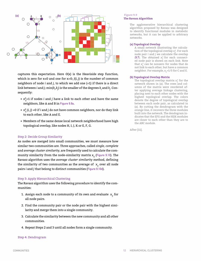
Step 1: Define the Similarity Matrix In an agglomerative algorithm similarity should be high for node pairs that belong to the same community and low for node pairs that belong to different communities. In a network context nodes that connect to each other and share neighbors likely belong to the same community, hence their xij should be large. The topological overlap matrix (Figure 9.9) [11]
(9.7)xoij = J (i, j)
min(ki, kj)+1‒Θ(Aij)
HIERARCHICAL CLUSTERING
HIERARCHICAL CLUSTERING12COMMUNITIES
captures this expectation. Here Θ(x) is the Heaviside step function, which is zero for x≤0 and one for x>0; J(i, j) is the number of common neighbors of node i and j, to which we add one (+1) if there is a direct link between i and j; min(ki,kj) is the smaller of the degrees ki and kj. Con-sequently:
• x0ij=1 if nodes i and j have a link to each other and have the same
neighbors, like A and B in Figure 9.9a.
• x0ij (i, j) =0 if i and j do not have common neighbors, nor do they link
to each other, like A and E.
• Members of the same dense local network neighborhood have high topological overlap, like nodes H, I, J, K or E, F, G.
Step 2: Decide Group Similarity As nodes are merged into small communities, we must measure how similar two communities are. Three approaches, called single, complete and average cluster similarity, are frequently used to calculate the com-munity similarity from the node-similarity matrix xij (Figure 9.10). The Ravasz algorithm uses the average cluster similarity method, defining the similarity of two communities as the average of xij over all node pairs i and j that belong to distinct communities (Figure 9.10d).
Step 3: Apply Hierarchical Clustering The Ravasz algorithm uses the following procedure to identify the com-munities:
1. Assign each node to a community of its own and evaluate xij for all node pairs.
2. Find the community pair or the node pair with the highest simi-larity and merge them into a single community.
3. Calculate the similarity between the new community and all other communities.
4. Repeat Steps 2 and 3 until all nodes form a single community.
Step 4: Dendrogram
The agglomerative hierarchical clustering algorithm proposed by Ravasz was designed to identify functional modules in metabolic networks, but it can be applied to arbitrary networks. (a) Topological Overlap
A small network illustrating the calcula-tion of the topological overlap xij
0. For each node pair i and j we calculate the overlap (9.7). The obtained xij
0 for each connect-ed node pair is shown on each link. Note that xij
0 can be nonzero for nodes that do not link to each other, but have a common neighbor. For example, xij
=1/3 for C and E.
(b) Topological Overlap Matrix The topological overlap matrix xij
0 for the network shown in (a). The rows and col-umns of the matrix were reordered af-ter applying average linkage clustering, placing next to each other nodes with the highest topological overlap. The colors denote the degree of topological overlap between each node pair, as calculated in (a). By cutting the dendrogram with the orange line, it recovers the three modules built into the network. The dendogram in-dicates that the EFG and the HIJK modules are closer to each other than they are to the ABC module.
After [11].
Figure 9.9The Ravasz Algorithm1
1 1
1/3
1/3
1 11
1
11
1/3
1/3 2/32/3
A B
C
D
IE
G
J
HK
F
archical tree according to the predominantbiochemical class of the substrates it produc-es, using the classification of metabolismbased on standard, small molecule biochem-
). As shown in Fig. 4A, and in thethree-dimensional representation in Fig. 4B,most substrates of a given small moleculeclass are distributed on the same branch ofthe tree (Fig. 4A) and correspond to relativelywell delimited regions of the metabolic net-work (Fig. 4B). Therefore, there are strongcorrelations between shared biochemicalclassification of metabolites and the globaltopological organization ofE. coli metabo-lism (Fig. 4A, bottom) (16).To correlate the putative modules ob-
tained from our graph theory–based analy-sis to actual biochemical pathways, we con-centrated on the pathways involving the
A
B
C
D
K
J
I
H
0.900.700.500.300.10
11 1
1/3
1/3
1 11
1
11
1/3
1/3 2/32/3
A (1) B(1)
C(3)
D(0)
I(1/3)E(1/3)
G (1/3)
J(2/3)
H(1/3)
K(1)F(1)
GFEHIJKDCBA
F
E
Fig. 3. Uncovering the underlyingmodularity of a complex network.(A) Topological overlap illustratedon a small hypothetical network. Foreach pair of nodes,i and j, we definethe topological overlapOT(i, j)J (i, j)/[min (k, k )], where J (i, j)
(a) (b)

HIERARCHICAL CLUSTERING13COMMUNITIES
The pairwise mergers of Step 3 will eventually pull all nodes into a sin-gle community. We can use a dendrogram to extract the underlying community organization.
The dendrogram visualizes the order in which the nodes are assigned to specific communities. For example, the dendrogram of Figure 9.9b tells us that the algorithm first merged nodes A with B, K with J and E with F, as each of these pairs have x0
ij=1. Next node C was added to the (A, B) community, I to (K, J) and G to (E, F).
To identify the communities we must cut the dendrogram. Hierarchical clustering does not tell us where that cut should be. Using for example the cut indicated as a dashed line in Figure 9.9b, we recover the three obvious communities (ABC, EFG, and HIJK).
Applied to the E. coli metabolic network (Figure 9.3a), the Ravasz algo-rithm identifies the nested community structure of bacterial me-tabolism. To check the biological relevance of these communities, we color-coded the branches of the dendrogram according to the known biochemical classification of each metabolite. As shown in Figure 9.3b, substrates with similar biochemical role tend to be located on the same branch of the tree. In other words the known biochemical classification of these metabolites confirms the biological relevance of the communi-ties extracted from the network topology.
Computational Complexity How many computations do we need to run the Ravasz algorithm? The
algorithm has four steps, each with its own computational complexity:
F
D
EB
A
C
G
F
D
EB
A
C
G
F
D
EB
A
C
G
A
C E
G
F
D
B
Single Linkage:
Average Linkage:Complete Linkage:
x12 = 1.59
x12 = 3.97 x12 = 2.84
1 2 1 2
1 21 2
D E F GA 2.75 2.22 3.46 3.08B 3.38 2.68 3.97 3.40C 2.31 1.59 2.88 2.34
x ij = rij =
F
D
EB
A
C
G
F
D
EB
A
C
G
F
D
EB
A
C
G
A
C E
G
F
D
B
Single Linkage:
Average Linkage:Complete Linkage:
x12 = 1.59
x12 = 3.97 x12 = 2.84
1 2 1 2
1 21 2
D E F GA 2.75 2.22 3.46 3.08B 3.38 2.68 3.97 3.40C 2.31 1.59 2.88 2.34
x ij = rij =
(a)
(c)
(b)
(d)
Figure 9.10Cluster Similarity
In agglomerative clustering we need to deter-mine the similarity of two communities from the node similarity matrix xij
. We illustrate this procedure for a set of points whose sim-ilarity xij
is the physical distance rij between
them. In networks xij corresponds to some
network-based distance measure, like xijo de-
fined in (9.7).
(a) Similarity MatrixSeven nodes forming two distinct com-munities. The table shows the distance rij
between each node pair, acting as the sim-ilarity xij
.
(b) Single Linkage Clustering The similarity between communities 1 and 2 is the smallest of all xij
, where i and j are in different communities. Hence the similarity is x12=1.59, corresponding to the distance between nodes C and E.
(c) Complete Linkage Clustering The similarity between two communities is the maximum of xij
, where i and j are in distinct communities. Hence x12=3.97.
(d) Average Linkage Clustering The similarity between two communities is the average of xij
over all node pairs i and j that belong to different communities. This is the procedure implemented in the Ravasz algorithm, providing x12=2.84.

HIERARCHICAL CLUSTERING14COMMUNITIES
Step 1: The calculation of the similarity matrix x0ij requires us to com-
pare N2 node pairs, hence the number of computations scale as N2. In other words its computational complexity is 0(N2).
Step 2: Group similarity requires us to determine in each step the dis-tance of the new cluster to all other clusters. Doing this N times re-quires 0(N2) calculations.
Steps 3 & 4: The construction of the dendrogram can be performed in 0(NlogN) steps.
Combining Steps 1-4, we find that the number of required computa-tions scales as 0(N2) + 0(N2) + 0(NlogN). As the slowest step scales as 0(N2), the algorithm’s computational complexity is 0(N2). Hence hierarchal clus-tering is much faster than the brute force approach, which generally scales as 0(eN).
DIVISIVE PROCEDURES: THE GIRVAN-NEWMAN ALGORITHMDivisive procedures systematically remove the links connecting nodes
that belong to different communities, eventually breaking a network into isolated communities. We illustrate their use by introducing an algorithm proposed by Michelle Girvan and Mark Newman [9,23], consisting of the following steps:
Step 1: Define Centrality While in agglomerative algorithms xij selects node pairs that belong to the same community, in divisive algorithms xij, called centrality, selects node pairs that are in different communities. Hence we want xij to be high (or low) if nodes i and j belong to different communities and small if they are in the same community. Three centrality measures that sat-isfy this expectation are discussed in Figure 9.11. The fastest of the three is link betweenness, defining xij as the number of shortest paths that go through the link (i, j). Links connecting different communities are expected to have large xij while links within a community have small xij.
Step 2: Hierarchical Clustering The final steps of a divisive algorithm mirror those we used in agglom-erative clustering (Figure 9.12):
1. Compute the centrality xij of each link.
2. Remove the link with the largest centrality. In case of a tie, choose one link randomly.
3. Recalculate the centrality of each link for the altered network.
0.29
0.29 0.57
0.31
0.31
0.17
0.17
0.2
0.2 0.4
0.23
0.23
0.18
0.18
0.29
0.29 0.57
0.31
0.31
0.17
0.17
0.2
0.2 0.4
0.23
0.23
0.18
0.18
Figure 9.11Centrality Measures
Divisive algorithms require a centrality mea-sure that is high for nodes that belong to dif-ferent communities and is low for node pairs in the same community. Two frequently used measures can achieve this:
(a) Link Betweenness Link betweenness captures the role of each link in information transfer. Hence xij
is proportional to the number of short-est paths between all node pairs that run along the link (i,j). Consequently, inter-community links, like the central link in the figure with xij
=0.57, have large betweenness. The calculation of link be-tweenness scales as 0(LN), or 0(N2) for a sparse network [23].
(b) Random-Walk Betweenness A pair of nodes m and n are chosen at random. A walker starts at m, following each adjacent link with equal probability until it reaches n. Random walk between-ness xij
is the probability that the link i→j was crossed by the walker after averaging over all possible choices for the starting nodes m and n. The calculation requires the inversion of an NxN matrix, with 0(N3) computational complexity and averaging the flows over all node pairs, with 0(LN2). Hence the total computational complexity of random walk betweenness is 0[(L + N)N2], or 0(N3) for a sparse network.
(a) (b)

HIERARCHICAL CLUSTERING15COMMUNITIES
4. Repeat steps 2 and 3 until all links are removed.
Girvan and Newman applied their algorithm to Zachary’s Karate Club (Figure 9.2a), finding that the predicted communities matched almost perfectly the two groups after the break-up. Only node 3 was classified incorrectly.
Computational Complexity The rate limiting step of divisive algorithms is the calculation of cen-
trality. Consequently the algorithm’s computational complexity depends on which centrality measure we use. The most efficient is link between-ness, with 0(LN) [24,25,26] (Figure 9.11a). Step 3 of the algorithm introduces an additional factor L in the running time, hence the algorithm scales as 0(L2N), or 0(N3) for a sparse network.
HIERARCHY IN REAL NETWORKSHierarchical clustering raises two fundamental questions:
Nested Communities First, it assumes that small modules are nested into larger ones. These nested communities are well captured by the dendrogram (Figures 9.9b and 9.12e). How do we know, however, if such hierarchy is indeed pres-ent in a network? Could this hierarchy be imposed by our algorithms, whether or not the underlying network has a nested community struc-ture?
Communities and the Scale-Free PropertySecond, the density hypothesis states that a network can be partitioned into a collection of subgraphs that are only weakly linked to other sub-graphs. How can we have isolated communities in a scale-free network, if the hubs inevitably link multiple communities?
D
J
A
C
B
K
E
HGI
FHF
E I
B
JKG
A
D
C
E
KI
A
H
C
D
F
B
GJ
BA
IF G
C
E
D
JKH
A B C D E F J H I J K
0
0.1
0.2
0.3
0.4
0.5
30 2 4 6 8 10
M
n
x
x
xD
J
A
C
B
K
E
HGI
FHF
E I
B
JKG
A
D
C
E
KI
A
H
C
D
F
B
GJ
BA
IF G
C
E
D
JKH
A B C D E F J H I J K
0
0.1
0.2
0.3
0.4
0.5
30 2 4 6 8 10
M
n
x
x
x
D
J
A
C
B
K
E
HGI
FHF
E I
B
JKG
A
D
C
E
KI
A
H
C
D
F
B
GJ
BA
IF G
C
E
D
JKH
A B C D E F J H I J K
0
0.1
0.2
0.3
0.4
0.5
30 2 4 6 8 10
M
n
x
x
xD
J
A
C
B
K
E
HGI
FHF
E I
B
JKG
A
D
C
E
KI
A
H
C
D
F
B
GJ
BA
IF G
C
E
D
JKH
A B C D E F J H I J K
0
0.1
0.2
0.3
0.4
0.5
30 2 4 6 8 10
M
n
x
x
x
D
J
A
C
B
K
E
HGI
FHF
E I
B
JKG
A
D
C
E
KI
A
H
C
D
F
B
GJ
BA
IF G
C
E
D
JKH
A B C D E F J H I J K
0
0.1
0.2
0.3
0.4
0.5
30 2 4 6 8 10
M
n
x
x
x
D
J
A
C
B
K
E
HGI
FHF
E I
B
JKG
A
D
C
E
KI
A
H
C
D
F
B
GJ
BA
IF G
C
E
D
JKH
A B C D E F J H I J K
0
0.1
0.2
0.3
0.4
0.5
30 2 4 6 8 10
M
n
x
x
x
(a) (b) (e)
(f) (c) (d)
Figure 9.12The Girvan-Newman Algorithm
(a) The divisive hierarchical algorithm of Gir-van and Newman uses link betweenness (Figure 9.11a) as centrality. In the figure the link weights, assigned proportionally to xij
, indicate that links connecting dif-ferent communities have the highest xij. Indeed, each shortest path between these communities must run through them.
(b)-(d) The sequence of images illustrates how the algorithm removes one-by-one the three highest xij
links, leaving three iso-lated communities behind. Note that be-tweenness needs to be recalculated after each link removal.
(e) The dendrogram generated by the Gir-van-Newman algorithm. The cut at level 3, shown as an orange dotted line, repro-duces the three communities present in the network.
(f) The modularity function, M, introduced in SECTION 9.4, helps us select the optimal cut. Its maxima agrees with our expecta-tion that the best cut is at level 3, as shown in (e).
HIERARCHICAL CLUSTERING16COMMUNITIES
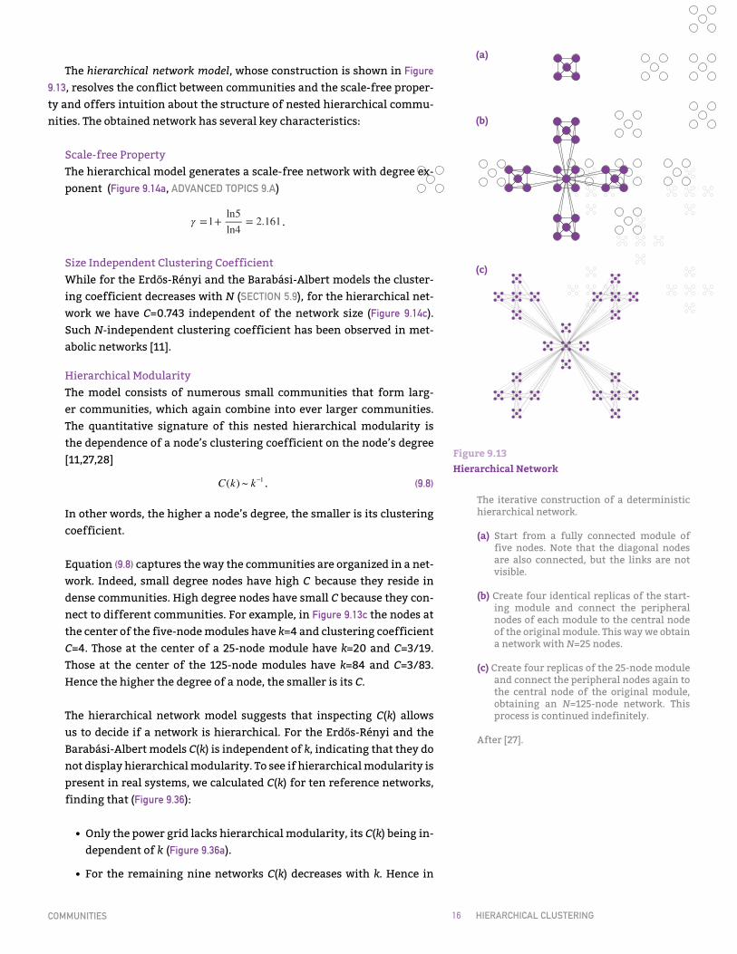
The hierarchical network model, whose construction is shown in Figure
9.13, resolves the conflict between communities and the scale-free proper-ty and offers intuition about the structure of nested hierarchical commu-nities. The obtained network has several key characteristics:
Scale-free Property The hierarchical model generates a scale-free network with degree ex-ponent (Figure 9.14a, ADVANCED TOPICS 9.A) .
Size Independent Clustering CoefficientWhile for the Erdős-Rényi and the Barabási-Albert models the cluster-ing coefficient decreases with N (SECTION 5.9), for the hierarchical net-work we have C=0.743 independent of the network size (Figure 9.14c). Such N-independent clustering coefficient has been observed in met-abolic networks [11].
Hierarchical ModularityThe model consists of numerous small communities that form larg-er communities, which again combine into ever larger communities. The quantitative signature of this nested hierarchical modularity is the dependence of a node’s clustering coefficient on the node’s degree [11,27,28]
. (9.8)
In other words, the higher a node’s degree, the smaller is its clustering coefficient.
Equation (9.8) captures the way the communities are organized in a net-work. Indeed, small degree nodes have high C because they reside in dense communities. High degree nodes have small C because they con-nect to different communities. For example, in Figure 9.13c the nodes at the center of the five-node modules have k=4 and clustering coefficient C=4. Those at the center of a 25-node module have k=20 and C=3/19. Those at the center of the 125-node modules have k=84 and C=3/83. Hence the higher the degree of a node, the smaller is its C.
The hierarchical network model suggests that inspecting C(k) allows us to decide if a network is hierarchical. For the Erdős-Rényi and the Barabási-Albert models C(k) is independent of k, indicating that they do not display hierarchical modularity. To see if hierarchical modularity is present in real systems, we calculated C(k) for ten reference networks, finding that (Figure 9.36):
• Only the power grid lacks hierarchical modularity, its C(k) being in-dependent of k (Figure 9.36a).
• For the remaining nine networks C(k) decreases with k. Hence in
γ =1+ ln5ln4 = 2.161
C(k) ~ k−1
(a)
(b)
(c)
Figure 9.13Hierarchical Network
The iterative construction of a deterministic hierarchical network.
(a) Start from a fully connected module of five nodes. Note that the diagonal nodes are also connected, but the links are not visible.
(b) Create four identical replicas of the start-ing module and connect the peripheral nodes of each module to the central node of the original module. This way we obtain a network with N=25 nodes.
(c) Create four replicas of the 25-node module and connect the peripheral nodes again to the central node of the original module, obtaining an N=125-node network. This process is continued indefinitely.
After [27].

HIERARCHICAL CLUSTERING17COMMUNITIES
these networks small nodes are part of small dense communities, while hubs link disparate communities to each other.
• For the scientific collaboration, metabolic, and citation network C(k) follows (9.8) in the high-k region. The form of C(k) for the In-ternet, mobile, email, protein interactions, and the WWW needs to be derived individually, as for those C(k) does not follow (9.8). More detailed network models predict C(k)~k-β, where β is between 0 and 2 [27,28].
In summary, in principle hierarchical clustering does not require pre-liminary knowledge about the number and the size of communities. In practice it generates a dendrogram that offers a family of community partitions characterizing the studied network. This dendrogram does not tell us which partition captures best the underlying community structure. Indeed, any cut of the hierarchical tree offers a potentially valid partition (Figure 9.15). This is at odds with our expectation that in each network there is a ground truth, corresponding to a unique community structure.
10 0 10 1 10 2 10 3 10 410 -8
10 -7
10 -6
10 -5
10 -4
10 -3
10 -2
10 -1
10 0
P(k)
10 0 10 1 10 2 10 3 10 4k10 -8
10 -7
10 -6
10 -5
10 -4
10 -3
10 -2
10 -1
10 0
P(k)
10 0 10 1 10 2 10 3 10 4 10 5k10 -4
10 -3
10 -2
10 -1
10 0
C(k)
10 2 10 3 10 4 10 5N10 -4
10 -3
10 -2
10 -1
10 0
C(N)pk
10 0 10 1 10 2 10 3 10 410 -8
10 -7
10 -6
10 -5
10 -4
10 -3
10 -2
10 -1
10 0
P(k)
10 0 10 1 10 2 10 3 10 4k10 -8
10 -7
10 -6
10 -5
10 -4
10 -3
10 -2
10 -1
10 0
P(k)
10 0 10 1 10 2 10 3 10 4 10 5k10 -4
10 -3
10 -2
10 -1
10 0
C(k)
10 2 10 3 10 4 10 5N10 -4
10 -3
10 -2
10 -1
10 0
C(N)pk
10 0 10 1 10 2 10 3 10 410 -8
10 -7
10 -6
10 -5
10 -4
10 -3
10 -2
10 -1
10 0
P(k)
10 0 10 1 10 2 10 3 10 4k10 -8
10 -7
10 -6
10 -5
10 -4
10 -3
10 -2
10 -1
10 0
P(k)
10 0 10 1 10 2 10 3 10 4 10 5k10 -4
10 -3
10 -2
10 -1
10 0
C(k)
10 2 10 3 10 4 10 5N10 -4
10 -3
10 -2
10 -1
10 0
C(N)pk
Figure 9.15Ambiguity in Hierarchical Clustering
Hierarchical clustering does not tell us where to cut a dendrogram. Indeed, depending on where we make the cut in the dendrogram of Figure 9.9a, we obtain (b) two, (c) three or (d) four communities. While for a small network we can visually decide which cut captures best the underlying community structure, it is im-possible to do so in larger networks. In the next section we discuss modularity, that helps us select the optimal cut.
Figure 9.14Scaling in Hierarchical Networks
Three quantities characterize the hierarchical network shown in Figure 9.13:
(a) Degree Distribution The scale-free nature of the generated network is illustrated by the scaling of pk with slope γ=ln 5/ln 4, shown as a dashed line. See ADVANCED TOPICS 9.A for the deri-vation of the degree exponent.
(b) Hierarchical ClusteringC(k) follows (9.8), shown as a dashed line. The circles show C(k) for a randomly wired scale-free network, obtained from the original model by degree-preserving ran-domization. The lack of scaling indicates that the hierarchical architecture is lost under rewiring. Hence C(k) captures a property that goes beyond the degree dis-tribution.
(c) Size Independent Clustering Coefficient The dependence of the clustering coef-ficient C on the network size N. For the hierarchical model C is independent of N (filled symbols), while for the Barabási-Al-bert model C(N) decreases (empty sym-bols).
After [27].
E
C
D
HI
A
GJ
F K
B
K
A
E
C
GF
D
HJ
I
B
K
A
E
C
GF
D
HJ
I
B
A B C D E F J H I J K
(a)
(a)
(b)
(b)
(c)
(c) (d)

HIERARCHICAL CLUSTERING18COMMUNITIES
While there are multiple notions of hierarchy in networks [29,30], in-specting C(k) helps decide if the underlying network has hierarchical mod-ularity. We find that C(k) decreases in most real networks, indicating that most real systems display hierarchical modularity. At the same time C(k) is independent of k for the Erdős-Rényi or Barabási-Albert models, indicating that these canonical models lack a hierarchical organization.

MODULARITYCOMMUNITIES 19
SECTION 9.4
In a randomly wired network the connection pattern between the nodes is expected to be uniform, independent of the network's degree distribu-tion. Consequently these networks are not expected to display systematic local density fluctuations that we could interpret as communities. This ex-pectation inspired the third hypothesis of community organization:
H3: Random Hypothesis
Randomly wired networks lack an inherent community structure.
This hypothesis has some actionable consequences: By comparing the link density of a community with the link density obtained for the same group of nodes for a randomly rewired network, we could decide if the original community corresponds to a dense subgraph, or its connectivity pattern emerged by chance.
In this section we show that systematic deviations from a random con-figuration allow us to define a quantity called modularity, that measures the quality of each partition. Hence modularity allows us to decide if a par-ticular community partition is better than some other one. Finally, modu-larity optimization offers a novel approach to community detection.
MODULARITYConsider a network with N nodes and L links and a partition into nc
communities, each community having Nc nodes connected to each other by Lc links, where c =1,...,nc. If Lc is larger than the expected number of links between the Nc nodes given the network’s degree sequence, then the nodes of the subgraph Cc could indeed be part of a true community, as expected based on the Density Hypothesis H2 (Figure 9.2). We therefore measure the difference between the network’s real wiring diagram (Aij) and the expect-ed number of links between i and j if the network is randomly wired (pij),
. (9.9)Mc = 12L ∑
(i, j)∈Cc
(Aij − pij)
MODULARITY

MODULARITY20COMMUNITIES
Here pij can be determined by randomizing the original network, while keeping the expected degree of each node unchanged. Using the degree preserving null model (7.1) we have
. (9.10)
If Mc is positive, then the subgraph Cc has more links than expected by chance, hence it represents a potential community. If Mc is zero then the connectivity between the Nc nodes is random, fully explained by the degree distribution. Finally, if Mc is negative, then the nodes of Cc do not form a community.
Using (9.10) we can derive a simpler form for the modularity (9.9) (AD-
VANCED TOPICS 9.B)
, (9.11)
where Lc is the total number of links within the community Cc and kc is the total degree of the nodes in this community.
To generalize these ideas to a full network consider the complete par-tition that breaks the network into nc communities. To see if the local link density of the subgraphs defined by this partition differs from the expect-ed density in a randomly wired network, we define the partition’s modu-larity by summing (9.11) over all nc communities [23]
. (9.12)
Modularity has several key properties:
• Higher Modularity Implies Better Partition The higher is M for a partition, the better is the corresponding com-munity structure. Indeed, in Figure 9.16a the partition with the maxi-mum modularity (M=0.41) accurately captures the two obvious com-munities. A partition with a lower modularity clearly deviates from these communities (Figure 9.16b). Note that the modularity of a parti-tion cannot exceed one [31,32].
• Zero and Negative Modularity By taking the whole network as a single community we obtain M=0, as in this case the two terms in the parenthesis of (9.12) are equal (Figure
9.16c). If each node belongs to a separate community, we have Lc=0 and the sum (9.12) has nc negative terms, hence M is negative (Figure
9.16d).
We can use modularity to decide which of the many partitions predict-ed by a hierarchical method offers the best community structure, select-ing the one for which M is maximal. This is illustrated in Figure 9.12f, which shows M for each cut of the dendrogram, finding a clear maximum when
pij =kikj
2L
Mc = Lc
L− ( kc
2L )2
M =nc
∑c=1
[ Lc
L− ( kc
2L )2
]
SINGLE COMMUNITYM = 0
OPTIMAL PARTITION SUBOPTIMAL PARTITION
NEGATIVE MODULARITY
M = 0 .22
M = − 0.12
M = 0 .41
SINGLE COMMUNITYM = 0
OPTIMAL PARTITION SUBOPTIMAL PARTITION
NEGATIVE MODULARITY
M = 0 .22
M = − 0.12
M = 0 .41
SINGLE COMMUNITYM = 0
OPTIMAL PARTITION SUBOPTIMAL PARTITION
NEGATIVE MODULARITY
M = 0 .22
M = − 0.12
M = 0 .41
SINGLE COMMUNITYM = 0
OPTIMAL PARTITION SUBOPTIMAL PARTITION
NEGATIVE MODULARITY
M = 0 .22
M = − 0.12
M = 0 .41
Figure 9.16Modularity
To better understand the meaning of modu-larity, we show M defined in (9.12) for several partitions of a network with two obvious com-munities.
(a) Optimal Partition The partition with maximal modularity M=0.41 closely matches the two distinct communities.
(b) Suboptimal Partition A partition with a sub-optimal but posi-tive modularity, M=0.22, fails to correctly identify the communities present in the network.
(c) Single Community If we assign all nodes to the same commu-nity we obtain M=0, independent of the network structure.
(d) Negative Modularity If we assign each node to a different com-munity, modularity is negative, obtaining M=-0.12.
(a)
(b)
(c)
(d)

MODULARITY21COMMUNITIES
the network breaks into three communities.
THE GREEDY ALGORITHM The expectation that partitions with higher modularity corresponds to
partitions that more accurately capture the underlying community struc-ture prompts us to formulate our final hypothesis:
H4: Maximal Modularity Hypothesis
For a given network the partition with maximum modularity corre-sponds to the optimal community structure.
The hypothesis is supported by the inspection of small networks, for which the maximum M agrees with the expected communities (Figures 9.12 and 9.16).
The maximum modularity hypothesis is the starting point of several community detection algorithms, each seeking the partition with the larg-est modularity. In principle we could identify the best partition by check-ing M for all possible partitions, selecting the one for which M is largest. Given, however, the exceptionally large number of partitions, this brute-force approach is computationally not feasible. Next we discuss an algo-rithm that finds partitions with close to maximal M, while bypassing the need to inspect all partitions.
Greedy AlgorithmThe first modularity maximization algorithm, proposed by Newman [33], iteratively joins pairs of communities if the move increases the partition's modularity. The algorithm follows these steps:
1. Assign each node to a community of its own, starting with N com-munities of single nodes.
2. Inspect each community pair connected by at least one link and compute the modularity difference ∆M obtained if we merge them. Identify the community pair for which ∆M is the largest and merge them. Note that modularity is always calculated for the full network.
3. Repeat Step 2 until all nodes merge into a single community, re-cording M for each step.
4. Select the partition for which M is maximal.
To illustrate the predictive power of the greedy algorithm consider the collaboration network between physicists, consisting of N=56,276 sci-entists in all branches of physics who posted papers on arxiv.org (Figure
9.17). The greedy algorithm predicts about 600 communities with peak modularity M = 0.713. Four of these communities are very large, togeth-er containing 77% of all nodes (Figure 9.17a). In the largest community 93% of the authors publish in condensed matter physics while 87% of the authors in the second largest community publish in high energy

MODULARITY22COMMUNITIES
physics, indicating that each community contains physicists of similar professional interests. The accuracy of the greedy algorithm is also il-lustrated in Figure 9.2a, showing that the community structure with the highest M for the Zachary Karate Club accurately captures the club’s subsequent split.
Computational Complexity Since the calculation of each ∆M can be done in constant time, Step 2 of the greedy algorithm requires O(L) computations. After deciding which communities to merge, the update of the matrix can be done in a worst-case time O(N). Since the algorithm requires N–1 community mergers, its complexity is O[(L + N)N], or O(N2) on a sparse graph. Optimized im-plementations reduce the algorithm’s complexity to O(Nlog2N) (ONLINE
RESOURCE 9.1).
LIMITS OF MODULARITYGiven the important role modularity plays in community identifica-
tion, we must be aware of some of its limitations.
Resolution Limit
Modularity maximization forces small communities into larger ones [34]. Indeed, if we merge communities A and B into a single community, the network’s modularity changes with (ADVANCED TOPICS 9.B)
, (9.13)
where lAB is number of links that connect the nodes in community A with total degree kA to the nodes in community B with total degree kB. If A and B are distinct communities, they should remain distinct when M is maximized. As we show next, this is not always the case.
Consider the case when kAkB|2L < 1, in which case (9.13) predicts ∆MAB
> 0 if there is at least one link between the two communities (lAB ≥ 1). Hence we must merge A and B to maximize modularity. Assuming for simplicity that kA ~ kB= k, if the total degree of the communities satisfies
ΔMAB = lAB
L− kAkB
2L2
+ 600 smaller communities
Physics E−print Archive, 56,276 nodes
11,070
87% H.E.P.
9,278
1,0091,0051,744
98% astro
9,35086% C.M.
93% C.M.
13,454
power−law distribution of group sizes
615480
460
mostly condensed matter, 9,350 nodes subgroup, 134 nodes
28 nodessingle research group
Figure 9.17The Greedy Algorithm
(a) Clustering Physicists The community structure of the collabo-ration network of physicists. The greedy algorithm predicts four large communi-ties, each composed primarily of phys-icists of similar interest. To see this on each cluster we show the percentage of members who belong to the same subfield of physics. Specialties are determined by the subsection(s) of the e-print archive in which individuals post papers. C.M. indi-cates condensed matter, H.E.P. high-ener-gy physics, and astro astrophysics. These four large communities coexist with 600 smaller communities, resulting in an overall modularity M=0.713.
(b) Identifying SubcommunitiesWe can identify subcommunities by applying the greedy algorithm to each community, treating them as separate networks. This procedure splits the con-densed matter community into many smaller subcommunities, increasing the modularity of the partition to M=0.807.
(c) Research GroupsOne of these smaller communities is fur-ther partitioned, revealing individual re-searchers and the research groups they belong to.
After [33].
(a) (b) (c)

MODULARITY23COMMUNITIES
(9.14)
then modularity increases by merging A and B into a single communi-ty, even if A and B are otherwise distinct communities. This is an arti-fact of modularity maximization: if kA and kB are under the threshold (9.14), the expected number of links between them is smaller than one. Hence even a single link between them will force the two communities together when we maximize M. This resolution limit has several conse-quences:
• Modularity maximization cannot detect communities that are smaller than the resolution limit (9.14). For example, for the WWW sample with L=1,497,134 (Table 2.1) modularity maximization will have difficulties resolving communities with total degree kC ≲
1,730.
• Real networks contain numerous small communities [36-38]. Giv-en the resolution limit (9.14), these small communities are system-atically forced into larger communities, offering a misleading characterization of the underlying community structure.
To avoid the resolution limit we can further subdivide the large com-munities obtained by modularity optimization [33,34,39]. For example, treating the smaller of the two condensed-matter groups of Figure 9.17a as a separate network and feeding it again into the greedy algorithm, we obtain about 100 smaller communities with an increased modulari-ty M = 0.807 (Figure 9.17b) [33].
Modularity Maxima
All algorithms based on maximal modularity rely on the assumption that a network with a clear community structure has an optimal par-tition with a maximal M [40]. In practice we hope that Mmax is an easy to find maxima and that the communities predicted by all other parti-tions are distinguishable from those corresponding to Mmax. Yet, as we show next, this optimal partition is difficult to identify among a large number of close to optimal partitions.
Consider a network composed of nc subgraphs with comparable link densities kC ≈ 2L/nc. The best partition should correspond to the one where each cluster is a separate community (Figure 9.18a), in which case M=0.867. Yet, if we merge the neighboring cluster pairs into a single community we obtain a higher modularity M=0.87 (Figure 9.18b). In general (9.13) and (9.14) predicts that if we merge a pair of clusters, we change modularity with
. (9.15)
In other words the drop in modularity is less than ∆M = −2/nc2. For a
network with nc = 20 communities, this change is at most ∆M = −0.005, tiny compared to the maximal modularity M≃0.87 (Figure 9.18b). As the
k ≤ 2L
ΔM = lAB
L− 2
n2c
>
Online Resource 9.1
Modularity-based Algorithms
There are several widely used community finding algorithms that maximize modular-ity.
Optimized Greedy Algorithm The use of data structures for sparse matrices can decrease the greedy algorithm’s computa-tional complexity to 0(Nlog2N) [35]. See http://cs.unm.edu/~aaron/research/fastmodulari-ty.htm for the code.
Louvain AlgorithmThe modularity optimization algorithm achieves a computational complexity of 0(L) [2]. Hence it allows us to identify commu-nities in networks with millions of nodes, as illustrated in Figure 9.1. The algorithm is de-scribed in ADVANCED TOPICS 9.C. See https://sites.google.com/site/findcommunities/ for the code. >
MODULARITY24COMMUNITIES
7
in the network, so too does the height of the modularityfunction. Further, the number of these structures k islimited mainly by the size of the network, since therecannot be more modular structures than nodes in thenetwork. In practical contexts, variations in n are very
Qmax and increasing n (or) will generally tend to increase Qmax . If the intention
is to compare modularity scores across networks, theseects must be accounted for in order to ensure a fair
Of course, the precise dependence ofQmax on n and kdepends on the particular network topology and how it
increases. For instance, in Appendix A,we derive the exact dependence for the ring network andcalculate precisely how many ofits degenerate solutions
. Because of this dependence,for any empirical network should
not typically be interpreted without a null expectation
M=0.867
M=0.871
M=0.80
MO
DU
LAR
ITY,
M
Figure 9.18Modularity Maxima
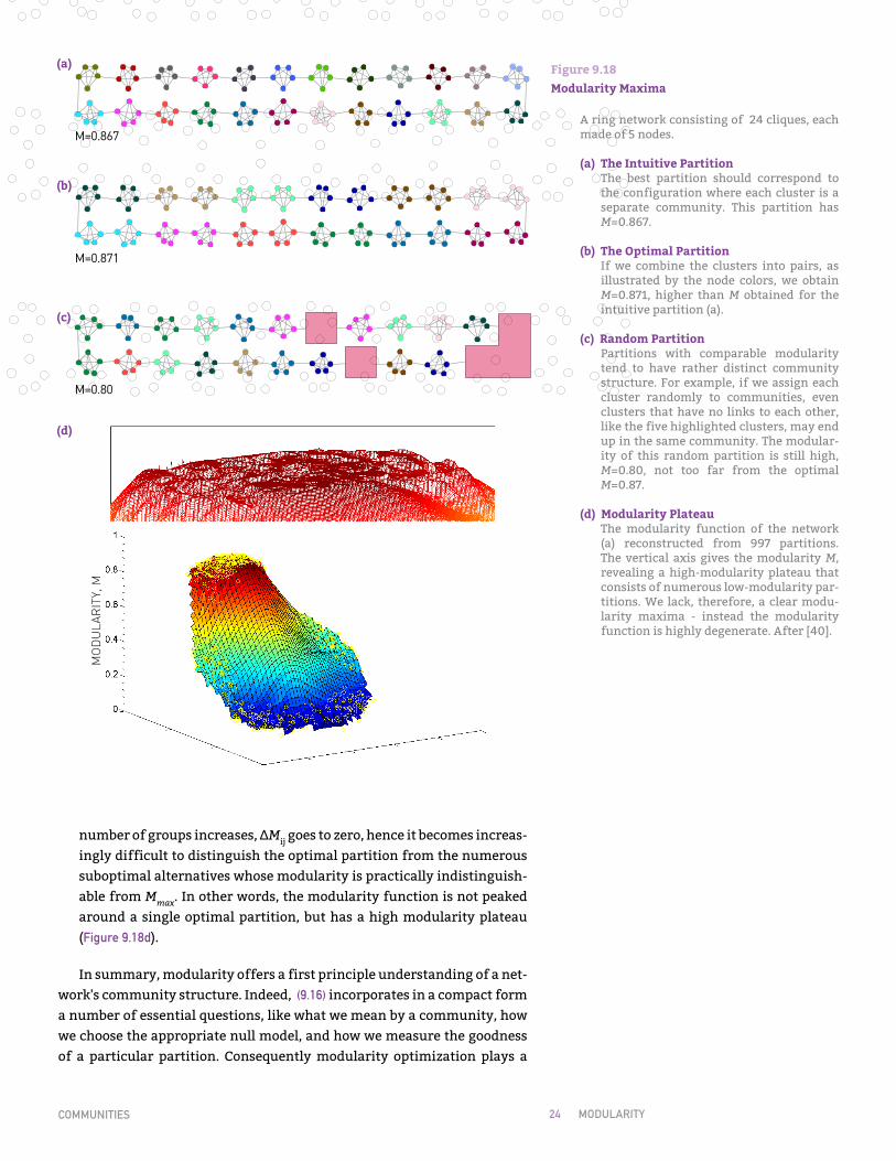
A ring network consisting of 24 cliques, each made of 5 nodes.
(a) The Intuitive PartitionThe best partition should correspond to the configuration where each cluster is a separate community. This partition has M=0.867.
(b) The Optimal PartitionIf we combine the clusters into pairs, as illustrated by the node colors, we obtain M=0.871, higher than M obtained for the intuitive partition (a).
(c) Random PartitionPartitions with comparable modularity tend to have rather distinct community structure. For example, if we assign each cluster randomly to communities, even clusters that have no links to each other, like the five highlighted clusters, may end up in the same community. The modular-ity of this random partition is still high, M=0.80, not too far from the optimal M=0.87.
(d) Modularity PlateauThe modularity function of the network (a) reconstructed from 997 partitions. The vertical axis gives the modularity M, revealing a high-modularity plateau that consists of numerous low-modularity par-titions. We lack, therefore, a clear modu-larity maxima - instead the modularity function is highly degenerate. After [40].
(a)
(b)
(c)
(d)
number of groups increases, ∆Mij goes to zero, hence it becomes increas-ingly difficult to distinguish the optimal partition from the numerous suboptimal alternatives whose modularity is practically indistinguish-able from Mmax. In other words, the modularity function is not peaked around a single optimal partition, but has a high modularity plateau (Figure 9.18d).
In summary, modularity offers a first principle understanding of a net-work's community structure. Indeed, (9.16) incorporates in a compact form a number of essential questions, like what we mean by a community, how we choose the appropriate null model, and how we measure the goodness of a particular partition. Consequently modularity optimization plays a
MODULARITY25COMMUNITIES
central role in the community finding literature.
At the same time, modularity has several well-known limitations: First, it forces together small weakly connected communities. Second, networks lack a clear modularity maxima, developing instead a modularity plateau containing many partitions with hard to distinguish modularity. This pla-teau explains why numerous modularity maximization algorithms can rapidly identify a high M partition: They identify one of the numerous par-titions with close to optimal M. Finally, analytical calculations and numer-ical simulations indicate that even random networks contain high mod-ularity partitions, at odds with the random hypothesis H3 that motivated the concept of modularity [41-43].
Modularity optimization is a special case of a larger problem: Finding communities by optimizing some quality function Q. The greedy algorithm and the Louvain algorithm described in ADVANCED TOPICS 9.C assume that Q = M, seeking partitions with maximal modularity. In ADVANCED TOPICS 9.C we also describe the Infomap algorithm, that finds communities by min-imizing the map equation L, an entropy-based measure of the partition quality [44-46].

OVERLAPPING COMMUNITIESCOMMUNITIES 26
SECTION 9.5
A node is rarely confined to a single community. Consider a scientist, who belongs to the community of scientists that share his professional in-terests. Yet, he also belongs to a community consisting of family members and relatives and perhaps another community of individuals sharing his hobby (Figure 9.19). Each of these communities consists of individuals who are members of several other communities, resulting in a complicated web of nested and overlapping communities [36]. Overlapping communities are not limited to social systems: The same genes are often implicated in multiple diseases, an indication that disease modules of different disor-ders overlap [14].
While the existence of a nested community structure has long been ap-preciated by sociologists [47] and by the engineering community interest-ed in graph partitioning, the algorithms discussed so far force each node into a single community. A turning point was the work of Tamás Vicsek and collaborators [36,48], who proposed an algorithm to identify overlap-ping communities, bringing the problem to the attention of the network science community. In this section we discuss two algorithms to detect overlapping communities, clique percolation and link clustering.
CLIQUE PERCOLATIONThe clique percolation algorithm, often called CFinder, views a commu-
nity as the union of overlapping cliques [36]:
• Two k-cliques are considered adjacent if they share k – 1 nodes (Figure
9.20b).
• A k-clique community is the largest connected subgraph obtained by the union of all adjacent k-cliques (Figure 9.20c).
• k-cliques that can not be reached from a particular k-clique belong to other k-clique communities (Figure 9.20c,d).
The CFinder algorithm identifies all cliques and then builds an Nclique x Nclique clique–clique overlap matrix O, where Nclique is the number of cliques and Oij is the number of nodes shared by cliques i and j (Figure 9.39). A typical
OVERLAPPING COMMUNITIES
COMMUNITIES
Figure 9.19Overlapping Communities
Schematic representation of the communities surrounding Tamás Vicsek, who introduced the concept of overlapping communities. A zoom into the scientific community illus-trates the nested and overlapping structure of the community characterizing his scientific interests. After [36].
>
Online Resource 9.2
CFinder
The CFinder software, allowing us to identify overlapping communities, can be downloaded from www.cfinder.org.
>

OVERLAPPING COMMUNITIES27COMMUNITIES
output of the CFinder algorithm is shown in Figure 9.21, displaying the com-munity structure of the word bright. In the network two words are linked to each other if they have a related meaning. We can easily check that the overlapping communities identified by the algorithm are meaningful: The word bright simultaneously belongs to a community containing light-re-lated words, like glow or dark; to a community capturing colors (yellow, brown); to a community consisting of astronomical terms (sun, ray); and to a community linked to intelligence (gifted, brilliant). The example also illustrates the difficulty the earlier algorithms would have in identifying communities of this network: they would force bright into one of the four communities and remove from the other three. Hence communities would be stripped of a key member, leading to outcomes that are difficult to in-terpret.
Could the communities identified by CFinder emerge by chance? To dis-tinguish the real k-clique communities from communities that are a pure consequence of high link density we explore the percolation properties of k-cliques in a random network [48]. As we discussed in CHAPTER 3, if a ran-dom network is sufficiently dense, it has numerous cliques of varying or-der. A large k-clique community emerges in a random network only if the connection probability p exceeds the threshold (ADVANCED TOPICS 9.D)
. (9.16)
Under pc(k) we expect only a few isolated k-cliques (Figure 9.22a). Once p ex-ceeds pc(k), we observe numerous cliques that form k-clique communities (Figure 9.22b). In other words, each k-clique community has its own thresh-old:
• For k =2 the k-cliques are links and (9.16) reduces to pc(k)~1/N, which
pc(k) = 1[(k − 1)N ]1/(k−1)
Figure 9.20The Clique Percolation Algorithm (CFinder)
To identify k=3 clique-communities we roll a triangle across the network, such that each subsequent triangle shares one link (two nodes) with the previous triangle.
(a)-(b) Rolling CliquesStarting from the triangle shown in green in (a), (b) illustrates the second step of the algorithm.
(c) Clique Communities for k=3The algorithm pauses when the final tri-angle of the green community is added. As no more triangles share a link with the green triangles, the green community has been completed. Note that there can be multiple k-clique communities in the same network. We illustrate this by show-ing a second community in blue. The fig-ure highlights the moment when we add the last triangle of the blue community. The blue and green communities overlap, sharing the orange node.
(d) Clique Communities for k=4k=4 community structure of a small net-work, consisting of complete four node subgraphs that share at least three nodes. Orange nodes belong to multiple commu-nities.
Images courtesy of Gergely Palla.
(a) (b)
(c) (d)
Figure 9.21Overlapping Communities
Communities containing the word bright in the South Florida Free Association network, whose nodes are words, connected by a link if their meaning is related. The community structure identified by the CFinder algorithm accurately describes the multiple meanings of bright, a word that can be used to refer to light, color, astronomical terms, or intelli-gence. After [36].

OVERLAPPING COMMUNITIES28COMMUNITIES
is the condition for the emergence of a giant connected component in Erdős–Rényi networks.
• For k = 3 the cliques are triangles (Figure 9.22a,b) and (9.16) predicts pc(k)~1/√2N.
In other words, k-clique communities naturally emerge in sufficiently dense networks. Consequently, to interpret the overlapping community structure of a network, we must compare it to the community structure obtained for the degree-randomized version of the original network.
Computational ComplexityFinding cliques in a network requires algorithms whose running time
grows exponentially with N. Yet, the CFinder community definition is based on cliques instead of maximal cliques, which can be identified in polynomial time [49]. If, however, there are large cliques in the network, it is more efficient to identify all cliques using an algorithm with O(eN) com-plexity [36]. Despite this high computational complexity, the algorithm is relatively fast, processing the mobile call network of 4 million mobile phone users in less then one day [50] (see also Figure 9.28).
LINK CLUSTERINGWhile nodes often belong to multiple communities, links tend to be
community specific, capturing the precise relationship that defines a node’s membership in a community. For example, a link between two in-dividuals may indicate that they are in the same family, or that they work together, or that they share a hobby, designations that only rarely overlap. Similarly, in biology each binding interaction of a protein is responsible for a different function, uniquely defining the role of the protein in the cell. This specificity of links has inspired the development of community finding algorithms that cluster links rather than nodes [51,52].
The link clustering algorithm proposed by Ahn, Bagrow and Lehmann [51] consists of the following steps:
Step 1: Define Link Similarity The similarity of a link pair is determined by the neighborhood of the nodes connected by them. Consider for example the links (i,k) and (j,k), connected to the same node k. Their similarity is defined as (Figure
9.23a-c)
, (9.17)
where n+(i) is the list of the neighbors of node i, including itself. Hence S measures the relative number of common neighbors i and j have. Con-sequently S=1 if i and j have the same neighbors (Figure 9.23c). The less is the overlap between the neighborhood of the two links, the smaller is S (Figure 9.23b).
S ((i,k),( j,k))=|n+(i) ∩ n+( j) ||n+(i) ∪ n+( j) |
Figure 9.22The Clique Percolation Algorithm (CFinder)
Random networks built with probabilities p=0.13 (a) and p=0.22 (b). As both p's are larg-er than the link percolation threshold (pc=1/N=0.05 for N=20), in both cases most nodes belong to a giant component.
(a) Subcritical CommunitiesThe 3-clique (triangle) percolation thresh-old is pc(3)=0.16 according to (9.16), hence at p=0.13 we are below it. Therefore, only two small 3-clique percolation clusters are observed, which do not connect to each other.
(b) Supercritical CommunitiesFor p=0.22 we are above pc(3), hence we ob-serve multiple 3-cliques that form a giant 3-clique percolation cluster (purple). This network also has a second overlapping 3-clique community, shown in green.
After [48].
(a)
(b)

OVERLAPPING COMMUNITIES29COMMUNITIES
Step 2: Apply Hierarchical Clustering The similarity matrix S allows us to use hierarchical clustering to iden-tify link communities (SECTION 9.3). We use a single-linkage procedure, iteratively merging communities with the largest similarity link pairs (Figure 9.10).
Taken together, for the network of Figure 9.23e, (9.17) provides the sim-ilarity matrix shown in (d). The single-linkage hierarchical clustering leads to the dendrogram shown in (d), whose cuts result in the link com-munities shown in (e) and the overlapping node communities shown in (f).
Figure 9.24 illustrates the community structure of the characters of Victor Hugo’s novel Les Miserables identified using the link clustering algorithm. Anyone familiar with the novel can convince themselves that the communities accurately represent the role of each character. Several characters are placed in multiple communities, reflecting their overlapping roles in the novel. Links, however, are unique to each com-munity.
Computational Complexity The link clustering algorithm involves two time-limiting steps: sim-
ilarity calculation and hierarchical clustering. Calculating the similarity (9.17) for a link pair with degrees ki and kj requires max(ki,kj) steps. For a scale-free network with degree exponent γ the calculation of similarity has complexity O(N2/(γ-1)), determined by the size of the largest node, kmax. Hier-archical clustering requires O(L2) time steps. Hence the algorithm's total
12
4
5
67
8
93
A B
a b
c
a b
cC
Figure 1: (A) The similarity measureS eik ejk between edgeseik andejk sharing nodek. For this example,n i n j12 and n i n j 4, giving S 1 3. Two simple cases: (B) an isolated (ka kb 1), connected triple (a,c,b) hasS 1 3, while (C) an isolated triangle hasS 1.
21
3
5
21
3
5
a
b
c
Figure 2: An example network with nodecommunities (a) and link communities (b).(c) The resulting link similarity matrix andlink dendrogram. Compare with main textFig. 1.
index [1]:
S eik ejkn i n j
n i n j(2)
An example illustration of this similarity measure is shown in Fig.1 (see Sec.4.1 for generalizations of
k
i j
k
i j
S ( (i,k), ( j,k)) = 1 S ( (i,k), ( j,k)) = 13
jk
i
12
4
5
67
8
933-4
2-4
1-4
2-3
1-2
1-3
4-7
5-6
4-6
4-5
7-9
7-8
8-9
Figure 9.23Identifying Link Communities
The link clustering algorithm identifies links with a similar topological role in a network. It does so by exploring the connectivity patterns of the nodes at the two ends of each link. In-spired by the similarity function of the Ravasz algorithm [4] (Figure 9.19), the algorithm aims to assign to high similarity S the links that connect to the same group of nodes.
(a) The similarity S of the (i,k) and (j,k) links connected to node k detects if the two links belong to the same group of nodes. Denot-ing with n+(i) the list of neighbors of node i, including itself, we obtain |n+(i)∪n+(j)| =12 and |n+(i)∩n+(j)| =4, resulting in S = 1/3 according to (9.17).
(b) For an isolated (ki = kj = 1) connected triple we obtain S = 1/3.
(c) For a triangle we have S = 1.
(d) The link similarity matrix for the network shown in (e) and (f). Darker entries corre-spond to link pairs with higher similarity S. The figure also shows the resulting link dendrogram.
(e) The link community structure predicted by the cut of the dendrogram shown as an or-ange dashed line in (d).
(f) The overlapping node communities derived from the link communities shown in (e).
After [51].
(a)
(d)
(b) (c)
(e)
(f)
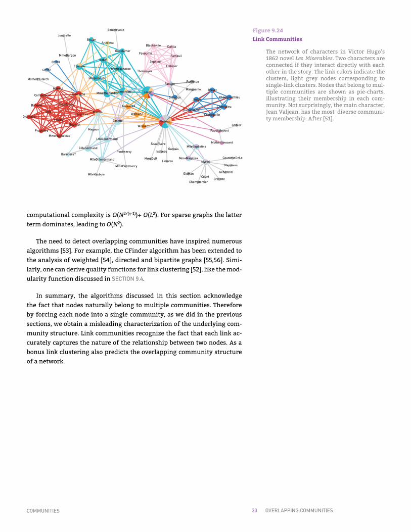
OVERLAPPING COMMUNITIES30COMMUNITIES
computational complexity is O(N2/(γ-1))+ O(L2). For sparse graphs the latter term dominates, leading to O(N2).
The need to detect overlapping communities have inspired numerous algorithms [53]. For example, the CFinder algorithm has been extended to the analysis of weighted [54], directed and bipartite graphs [55,56]. Simi-larly, one can derive quality functions for link clustering [52], like the mod-ularity function discussed in SECTION 9.4.
In summary, the algorithms discussed in this section acknowledge the fact that nodes naturally belong to multiple communities. Therefore by forcing each node into a single community, as we did in the previous sections, we obtain a misleading characterization of the underlying com-munity structure. Link communities recognize the fact that each link ac-curately captures the nature of the relationship between two nodes. As a bonus link clustering also predicts the overlapping community structure of a network.
Gavroche
ValjeanBossuet
Mabeuf
Bahorel
Grantaire
Gervais
FaucheleventGribier
Fameuil
Listolier
Thenardier
Bamatabois
Champmathieu
MmeHucheloup
Montparnasse
Courfeyrac
Enjolras
Gillenormand
Fantine
Tholomyes
MariusJoly
Brujon
GueulemerFavourite
ZephineEponine
MmeMagloireMyriel
MmeThenardier
Cosette
LtGillenormand
MlleGillenormand
Feuilly
MlleBaptistine
Blacheville
Claquesous
CombeferreJavert
Woman1
Dahlia
Child1
Child2
Perpetue
Simplice
Babet
Pontmercy
Chenildieu
Napoleon
CravatteChamptercier
Scaufflaire
Boulatruelle
Labarre
Judge
BaronessTCountessDeLo
Isabeau
Marguerite Brevet
Cochepaille
MmePontmercy
MlleVaubois
Magnon
Woman2
Prouvaire
MmeDeR
Toussaint
Count
MotherPlutarch
MmeBurgon
MotherInnocent
Anzelma
OldMan
Jondrette
Geborand
Figure 9.24Link Communities
The network of characters in Victor Hugo’s 1862 novel Les Miserables. Two characters are connected if they interact directly with each other in the story. The link colors indicate the clusters, light grey nodes corresponding to single-link clusters. Nodes that belong to mul-tiple communities are shown as pie-charts, illustrating their membership in each com-munity. Not surprisingly, the main character, Jean Valjean, has the most diverse communi-ty membership. After [51].

TESTING COMMUNITIESCOMMUNITIES 31
SECTION 9.6
Community identification algorithms offer a powerful diagnosis tool, al-lowing us to characterize the local structure of real networks. Yet, to inter-pret and use the predicted communities, we must understand the accuracy of our algorithms. Similarly, the need to diagnose large networks prompts us to address the computational efficiency of our algorithms. In this sec-tion we focus on the concepts needed to assess the accuracy and the speed of community finding.
ACCURACYIf the community structure is uniquely encoded in the network’s wiring diagram, each algorithm should predict precisely the same communities. Yet, given the different hypotheses the various algorithms embody, the partitions uncovered by them can differ, prompting the question: Which community finding algorithm should we use? To assess the performance of community finding algorithms we need to measure an algorithm’s accuracy, i.e. its ability to uncover communities in networks whose community structure is known. We start by discussing two benchmarks, which are networks with predefined community struc-ture, that we can use to test the accuracy of a community finding algo-rithm.
Girvan-Newman (GN) BenchmarkThe Girvan-Newman benchmark consists of N=128 nodes partitioned into nc=4 communities of size Nc=32 [9,57]. Each node is connected with probability pint to the Nc–1 nodes in its community and with probability pext to the 3Nc nodes in the other three communities. The control pa-rameter
, (9.18)
captures the density differences within and between communities. We
μ = kext
kext + kint
TESTING COMMUNITIES
COMMUNITIES

TESTING COMMUNITIES32COMMUNITIES
0
0.2
0.4
0.6
0.8
1
0.1 0.2 0.3 0.4 0.5 0.6
In
µ
Ravasz
(a)
(b)
(c)
Figure 9.25Testing Accuracy with the NG Benchmark
The position of each node in (a) and (c) shows the planted communities of the Girvan-New-man (GN) benchmark, illustrating the pres-ence of four distinct communities, each with Nc=32 nodes.
(a) The node colors represent the partitions predicted by the Ravasz algorithm for mixing parameter µ=0.40 given by (9.18). As in this case the communities are well separated, we have an excellent agree-ment between the planted and the detect-ed communities.
(b) The normalized mutual information in function of the mixing parameter µ for the Ravasz algorithm. For small µ we have In≃1 and nc≃4, indicating that the algorithm can easily detect well separated commu-nities, as illustrated in (a). As we increase µ the link density difference within and between communities becomes less pro-nounced. Consequently the communities are increasingly difficult to identify and In decreases.
(c) For µ=0.50 the Ravasz algorithm misplaces a notable fraction of the nodes, as in this case the communities are not well sepa-rated, making it harder to identify the cor-rect community structure.
Note that the Ravasz algorithm generates mul-tiple partitions, hence for each µ we show the partition with the largest modularity, M. Next to (a) and (c) we show the normalized mutual information associated with the correspond-ing partition and the number of detected com-munities nc. The normalized mutual informa-tion (9.23), developed for non-overlapping communities, can be extended to overlapping communities as well [59].
expect community finding algorithms to perform well for small µ (Fig-
ure 9.25a), when the probability of connecting to nodes within the same community exceeds the probability of connecting to nodes in different communities. The performance of all algorithms should drop for large µ (Figure 9.25b), when the link density within the communities becomes comparable to the link density in the rest of the network.
Lancichinetti-Fortunato-Radicchi (LFR) BenchmarkThe GN benchmark generates a random graph in which all nodes have comparable degree and all communities have identical size. Yet, the de-gree distribution of most real networks is fat tailed, and so is the com-munity size distribution (Figure 9.29). Hence an algorithm that performs well on the GN benchmark may not do well on real networks. To avoid

TESTING COMMUNITIES33COMMUNITIES
this limitation, the LFR benchmark (Figure 9.26) builds networks for which both the node degrees and the planted community sizes follow power laws [58].
Having built networks with known community structure, next we need tools to measure the accuracy of the partition predicted by a particular community finding algorithm. As we do so, we must keep in mind that the two benchmarks discussed above correspond to a particular definition of communities. Consequently algorithms based on clique percolation or link clustering, that embody a different notion of communities, may not fare so well on these.
Measuring AccuracyTo compare the predicted communities with those planted in the bench-
mark, consider an arbitrary partition into non-overlapping communities. In each step we randomly choose a node and record the label of the com-munity it belongs to. The result is a random string of community labels that follow a p(C) distribution, representing the probability that a random-ly selected node belongs to the community C.
Consider two partitions of the same network, one being the benchmark (ground truth) and the other the partition predicted by a community find-ing algorithm. Each partition has its own p(C1) and p(C2) distribution. The joint distribution, p(C1, C2), is the probability that a randomly chosen node belongs to community C1 in the first partition and C2 in the second. The similarity of the two partitions is captured by the normalized mutual in-formation [38]
. (9.19)
The numerator of (9.19) is the mutual information I, measuring the in-formation shared by the two community assignments: I=0 if C1 and C2 are independent of each other; I equals the maximal value H({p(C1)}) = H({p(C2)}) when the two partitions are identical and
(9.20)
In =∑
C1,C2
p(C1, C2)log2p(C1, C2)
p(C1)p(C2)
12 H({p(C1)}) + 1
2 H({p(C2)})
H({p(C )}) = − ∑C
p(C )log2 p(C )
(a)
(b)
(c)
(d)
(e) Figure 9.26LFR Benchmark
The construction of the Lancichinetti-Fortu-nato-Radicchi (LFR) benchmark, which gener-ates networks in which both the node degrees and community sizes follow a power law. The benchmark is built as follows [57]:
(a) Start with N isolated nodes.
(b) Assign each node to a community of size Nc where Nc follows the power law distri-bution PNc
~Nc-ζ with community exponent
ζ. Also assign each node i a degree ki select-ed from the power law distribution pk~k -γ with degree exponent γ.
(c) Each node i of a community receives an in-ternal degree (1-µ)ki, shown as links whose color agrees with the node color. The re-maining µki degrees, shown as black links, connect to nodes in other communities.
(d) All stubs of nodes of the same community are randomly attached to each other, until no more stubs are ‘‘free’’. In this way we maintain the sequence of internal degrees of each node in its community. The re-maining µki stubs are randomly attached to nodes from other communities.
(e) A typical network and its community struc-ture generated by the LFR benchmark with N=500, γ=2.5, and ζ=2.
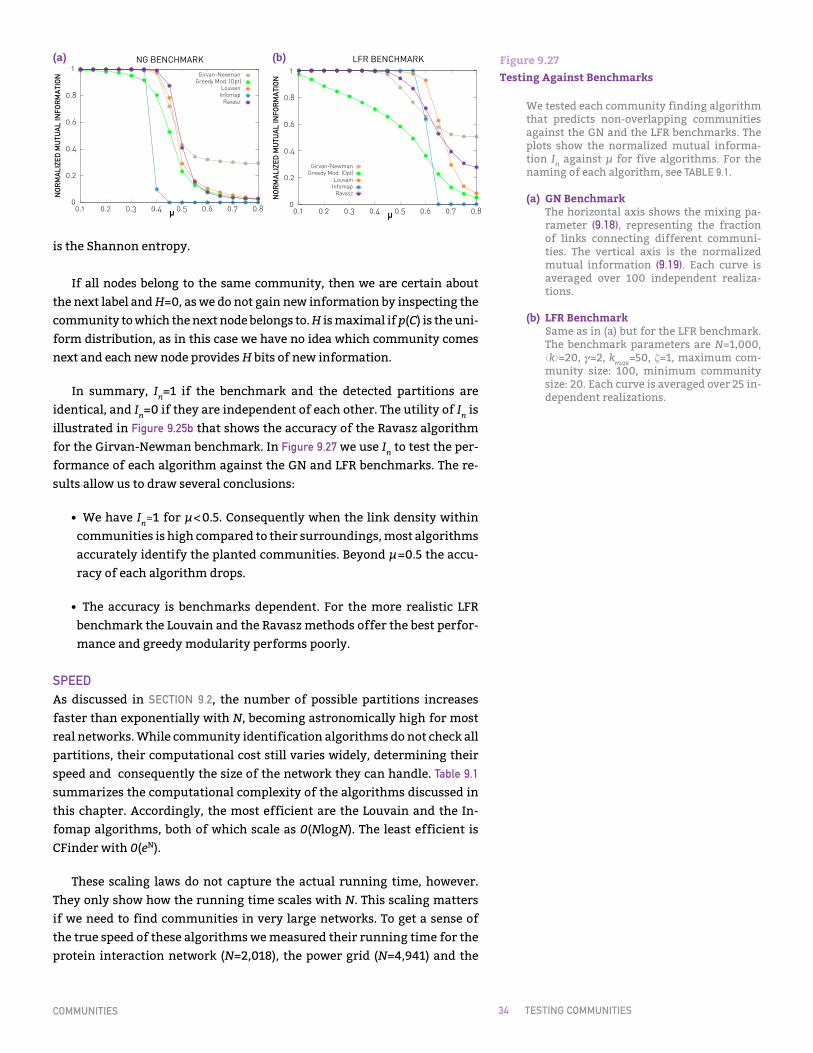
TESTING COMMUNITIES34COMMUNITIES
is the Shannon entropy.
If all nodes belong to the same community, then we are certain about the next label and H=0, as we do not gain new information by inspecting the community to which the next node belongs to. H is maximal if p(C) is the uni-form distribution, as in this case we have no idea which community comes next and each new node provides H bits of new information.
In summary, In=1 if the benchmark and the detected partitions are identical, and In=0 if they are independent of each other. The utility of In is illustrated in Figure 9.25b that shows the accuracy of the Ravasz algorithm for the Girvan-Newman benchmark. In Figure 9.27 we use In to test the per-formance of each algorithm against the GN and LFR benchmarks. The re-sults allow us to draw several conclusions:
• We have In≃1 for µ<0.5. Consequently when the link density within communities is high compared to their surroundings, most algorithms accurately identify the planted communities. Beyond µ=0.5 the accu-racy of each algorithm drops.
• The accuracy is benchmarks dependent. For the more realistic LFR benchmark the Louvain and the Ravasz methods offer the best perfor-mance and greedy modularity performs poorly.
SPEEDAs discussed in SECTION 9.2, the number of possible partitions increases faster than exponentially with N, becoming astronomically high for most real networks. While community identification algorithms do not check all partitions, their computational cost still varies widely, determining their speed and consequently the size of the network they can handle. Table 9.1 summarizes the computational complexity of the algorithms discussed in this chapter. Accordingly, the most efficient are the Louvain and the In-fomap algorithms, both of which scale as 0(NlogN). The least efficient is CFinder with 0(eN).
These scaling laws do not capture the actual running time, however. They only show how the running time scales with N. This scaling matters if we need to find communities in very large networks. To get a sense of the true speed of these algorithms we measured their running time for the protein interaction network (N=2,018), the power grid (N=4,941) and the
NG BENCHMARK
LFR BENCHMARK
Girvan-NewmanGreedy Mod. (Opt)
LouvainInfomap
Ravasz
0
0.2
0.4
0.6
0.8
1
0.1 0.2 0.3 0.4 0.5 0.6 0.7 0.8µ
NORM
ALIZ
ED M
UTUA
L IN
FORM
ATIO
N
Girvan-NewmanGreedy Mod. (Opt)
LouvainInfomap
Ravasz
0
0.2
0.4
0.6
0.8
1
0.1 0.2 0.3 0.4 0.5 0.6 0.7 0.8µ
NORM
ALIZ
ED M
UTUA
L IN
FORM
ATIO
N
(a) (b) Figure 9.27Testing Against Benchmarks
We tested each community finding algorithm that predicts non-overlapping communities against the GN and the LFR benchmarks. The plots show the normalized mutual informa-tion In against µ for five algorithms. For the naming of each algorithm, see TABLE 9.1.
(a) GN Benchmark The horizontal axis shows the mixing pa-rameter (9.18), representing the fraction of links connecting different communi-ties. The vertical axis is the normalized mutual information (9.19). Each curve is averaged over 100 independent realiza-tions.
(b) LFR BenchmarkSame as in (a) but for the LFR benchmark. The benchmark parameters are N=1,000, ⟨k⟩=20, γ=2, kmax=50, ζ=1, maximum com-munity size: 100, minimum community size: 20. Each curve is averaged over 25 in-dependent realizations.
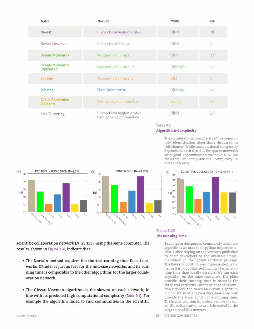
TESTING COMMUNITIES35COMMUNITIES
NAME NATURE COMP. REF
Ravasz
Girvan-Newman
Greedy Modularity
Greedy Modularity
Louvain
Infomap
Clique Percolation
Link Clustering
Hierarchical Agglomerative
Hierarchical Divisive
Modularity Optimization
Modularity Optimization
Modularity Optimization
Flow Optimization
Overlapping Communities
Hierarchical Agglomerative;Overlapping Communities
O(N2)
O(N3)
O(N2)
O(Nlog2N)
O(L)
O(NlogN)
Exp(N)
O(N2)
[11]
[9]
[33]
[35]
[2]
[44]
[48]
[51]
(CFinder)
(Optimized)
Table 9.1Algorithmic Complexity
The computational complexity of the commu-nity identification algorithms discussed in this chapter. While computational complexity depends on both N and L, for sparse networks with good approximation we have L~N. We therefore list computational complexity in terms of N only.
scientific collaboration network (N=23,133), using the same computer. The results, shown in Figure 9.28, indicate that:
• The Louvain method requires the shortest running time for all net-works. CFinder is just as fast for the mid-size networks, and its run-ning time is comparable to the other algorithms for the larger collab-oration network.
• The Girvan-Newman algorithm is the slowest on each network, in line with its predicted high computational complexity (Table 9.1). For example the algorithm failed to find communities in the scientific
Figure 9.28The Running Time
To compare the speed of community detection algorithms we used their python implementa-tion, either relying on the versions published by their developers or the available imple-mentation in the igraph software package. The Ravasz algorithm was implemented by us, hence it is not optimized, having a larger run-ning time than ideally possible. We ran each algorithm on the same computer. The plots provide their running time in seconds for three real networks. For the science collabora-tion network the Newman-Girvan algorithm did not finish after seven days, hence we only provide the lower limit of its running time. The higher running time observed for the sci-entific collaboration network is rooted in the larger size of this network.
10-2
10-1
100
101
102
103
t[s]
Newman-Girvan
Greedy Mod. (Opt.)
Louvain
Infomap
Ravasz
CFinder
Link
10-2
10-1
100
101
102
103
t[s]
Newman-Girvan
Greedy Mod. (Opt.)
Louvain
Infomap
Ravasz
CFinder
Link
10-2
10-1
100
101
102
103
104
105
t[s]
Newman-Girvan
Greedy Mod. (Opt.)
Louvain
Infomap
Ravasz
CFinder
Link
PROTEIN INTERACTIONs (N=2,018)
SCIENTIFIC COLLABORATION (N=4,941)
POWER GRID (N=23,133)
10-2
10-1
100
101
102
103
t[s]
Newman-Girvan
Greedy Mod. (Opt.)
Louvain
Infomap
Ravasz
CFinder
Link
10-2
10-1
100
101
102
103
t[s]
Newman-Girvan
Greedy Mod. (Opt.)
Louvain
Infomap
Ravasz
CFinder
Link
10-2
10-1
100
101
102
103
104
105
t[s]
Newman-Girvan
Greedy Mod. (Opt.)
Louvain
Infomap
Ravasz
CFinder
Link
PROTEIN INTERACTIONs (N=2,018)
SCIENTIFIC COLLABORATION (N=4,941)
POWER GRID (N=23,133)
(a) (b) (c)

TESTING COMMUNITIES36COMMUNITIES
collaboration network in seven days.
In summary, benchmarks allow us to compare the accuracy and the speed of the available algorithms. Given that the development of the fast-est and the most accurate community detection tool remains an active arms race, those interested in the subject should consult the literature that compares algorithms across multiple dimensions [31,58,60,61].

CHARACTERIZING COMMUNITIESCOMMUNITIES 37
SECTION 9.7
CHARACTERIZING COMMUNITIES
COMMUNITIES
Research in network science is driven by the desire to quantify the fundamental principles that govern how networks emerge and how they are organized. These organizing principles impact the structure of com-munities, as well as our ability to identify them. In this section we discuss community evolution, the characteristics of community size distribution and the role of the link weights in community identification, allowing us to uncover the generic principles of community organization.
COMMUNITY SIZE DISTRIBUTION According to the fundamental hypothesis (H1) the number and the size
of communities in a network are uniquely determined by the network’s wiring diagram. We must therefore ask: What is the size distribution of these communities?
Many studies report fat tailed community size distributions, imply-ing that numerous small communities coexist with a few very large ones [16,33,35,36,60]. To explore how widespread this pattern is, in Figure 9.29 we show pNc
for three networks, as predicted by various community finding algorithms. The plots indicate several patterns:
• For the protein interaction and the science collaboration network all algorithms predict an approximately fat tailed pNc
. Hence in these net-works numerous tiny communities coexist with a few large commu-nities.
• For the power grid different algorithms lead to distinct outcomes. Modularity-based algorithms predict communities with comparable size Nc ≃ 102. In contrast, the Ravasz algorithm and Infomap predict numerous communities with size Nc ≃ 10 and a few larger communi-ties. Finally, clique percolation and link clustering predict an approxi-mately fat tailed community size distribution.
These differences suggest that the fat tailed community size distribu-tion is not a byproduct of a particular algorithm. Rather it is an inherent
Figure 9.29Community Size Distribution
The community size distribution pNc predicted
by the community finding algorithms explored in this chapter. The name convention for the al-gorithms is shown in Table 9.1. For the protein interaction (a) and the scientific collaboration network (b) all algorithms predict an approxi-mately fat-tailed community size distribution, hence the predictions are more-or-less consis-tent with each other. The algorithms offer con-flicting results for the power grid, shown in (c).
10-4
10-3
10-2
10-1
100
100 101 10 2 103
Girvan-NewmanGreedyModOpt
LouvainInfomapRavaszCFinder
Link
PROTEIN INTERACTIONS
Nc
NcP
10-4
10-5
10-3
10-2
10-1
100
100 101 10 2 10 3 103104
GreedyModOptLouvainInfomapRavaszCFinder
Link
SCIENTIFIC COLLABORATION
Nc
NcP
10-4
10-3
10-2
10-1
100
100 101 10 2 103
Girvan-NewmanGreedyModOpt
LouvainInfomapRavaszCFinder
Link
POWER GRID
Nc
NcP
10-4
10-3
10-2
10-1
100
100 101 10 2 103
Girvan-NewmanGreedyModOpt
LouvainInfomapRavaszCFinder
Link
PROTEIN INTERACTIONS
Nc
NcP
10-4
10-5
10-3
10-2
10-1
100
100 101 10 2 10 3 103104
GreedyModOptLouvainInfomapRavaszCFinder
Link
SCIENTIFIC COLLABORATION
Nc
NcP
10-4
10-3
10-2
10-1
100
100 101 10 2 103
Girvan-NewmanGreedyModOpt
LouvainInfomapRavaszCFinder
Link
POWER GRID
Nc
NcP
(c)
(b)
(a)

CHARACTERIZING COMMUNITIES38COMMUNITIES
property of some networks, like the protein and the scientific collabora-tion network. The different outcomes for the power grid suggests that this network lacks a unique and detectable community structure.
COMMUNITIES AND LINK WEIGHTSLink weights are deeply correlated with the community structure. Yet,
as we discuss next, the nature of these correlations is system dependent.
Social Networks The more time two individuals spend together, the more likely that they share friends, which increases the chance that they belong to the same community. Consequently communities in social networks tend to be nucleated around strong ties. Links connecting different communities are weaker in comparison. This pattern, known as the weak tie hypoth-esis [62], is illustrated in Figure 9.30a for the mobile call network [63]. We observe that strong ties are indeed predominantly within the numer-ous small communities, and links connecting communities are visibly weaker.
Transport SystemsThe purpose of many technological and biological networks is to trans-port materials or information. In this case the link weights are expect-ed to correlate with betweenness centrality [64,65,66], a proxy of the local traffic carried by a network. As links connecting different com-munities must transport considerable amount of traffic, in transport networks strong ties are between communities. In contrast links within communities are weaker in comparison (Figure 9.30b).
The coupling between link weights and community structure suggests that incorporating the link weights could enhance the accuracy of commu-nity finding algorithms. Yet, the different nature of the coupling in social and technological systems serves as a cautionary note: Algorithms that aim to place in the same community nodes connected by strong ties may be only effective in social systems. They may offer potentially misleading results in technological and biological systems, where strong ties connect different communities.
COMMUNITY EVOLUTIONChanges in a network’s wiring diagram can have multiple consequenc-
es for communities: they can lead to the birth of new communities, the growth or the contraction of the existing communities, communities can merge with each other or split into several smaller communities, and fi-nally communities can die (Figure 9.31) [50]. Studies focusing on social and communication networks offer several insights into the changes commu-nities experience [50,67-73]:
Growth
B
C
A
B
1
10010
Figure 9.30Communities and Link Weights
The mobile call network helps us illustrate the relationship between link weights and communities. Links represent mutual calls between the users. We show only nodes that are at distance six or less from the individual highlighted as a black circle in (a).
(a) Real WeightsThe link colors capture the aggregate call duration in minutes (see color bar). In line with the weak tie hypothesis we find strong ties mainly within communities and weak ties between communities [62].
(b) Betweenness CentralityIf the link weights are driven by the need to transport information or materials, as it is often the case in technological and biological systems, the weights are well approximated by betweenness centrality (Figure 9.11). We colored the links based on each link’s betweenness centrality. As the figure indicates, links connecting commu-nities have high betweenness (red), where-as the links within communities have low betweenness (green).
After [63].
(a)
(b)
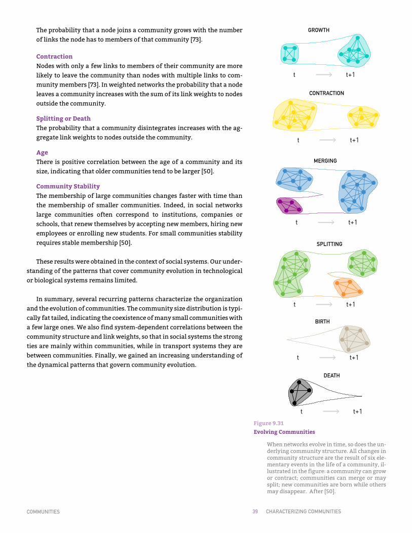
CHARACTERIZING COMMUNITIES39COMMUNITIES
The probability that a node joins a community grows with the number of links the node has to members of that community [73].
ContractionNodes with only a few links to members of their community are more likely to leave the community than nodes with multiple links to com-munity members [73]. In weighted networks the probability that a node leaves a community increases with the sum of its link weights to nodes outside the community.
Splitting or DeathThe probability that a community disintegrates increases with the ag-gregate link weights to nodes outside the community.
AgeThere is positive correlation between the age of a community and its size, indicating that older communities tend to be larger [50].
Community StabilityThe membership of large communities changes faster with time than the membership of smaller communities. Indeed, in social networks large communities often correspond to institutions, companies or schools, that renew themselves by accepting new members, hiring new employees or enrolling new students. For small communities stability requires stable membership [50].
These results were obtained in the context of social systems. Our under-standing of the patterns that cover community evolution in technological or biological systems remains limited.
In summary, several recurring patterns characterize the organization and the evolution of communities. The community size distribution is typi-cally fat tailed, indicating the coexistence of many small communities with a few large ones. We also find system-dependent correlations between the community structure and link weights, so that in social systems the strong ties are mainly within communities, while in transport systems they are between communities. Finally, we gained an increasing understanding of the dynamical patterns that govern community evolution.
GROWTH
t t+1
MERGING SPLITTING
BIRTH DEATH
CONTRACTION
t t+1
t t+1t t+1
t t+1
t t+1
GROWTH
t t+1
MERGING SPLITTING
BIRTH DEATH
CONTRACTION
t t+1
t t+1t t+1
t t+1
t t+1
GROWTH
t t+1
MERGING SPLITTING
BIRTH DEATH
CONTRACTION
t t+1
t t+1t t+1
t t+1
t t+1
GROWTH
t t+1
MERGING SPLITTING
BIRTH DEATH
CONTRACTION
t t+1
t t+1t t+1
t t+1
t t+1
GROWTH
t t+1
MERGING SPLITTING
BIRTH DEATH
CONTRACTION
t t+1
t t+1t t+1
t t+1
t t+1GROWTH
t t+1
MERGING SPLITTING
BIRTH DEATH
CONTRACTION
t t+1
t t+1t t+1
t t+1
t t+1
Figure 9.31Evolving Communities
When networks evolve in time, so does the un-derlying community structure. All changes in community structure are the result of six ele-mentary events in the life of a community, il-lustrated in the figure: a community can grow or contract; communities can merge or may split; new communities are born while others may disappear. After [50].

SUMMARYCOMMUNITIES 40
SECTION 9.8
The ubiquity of communities across different networks has turned community identification into a dynamically developing chapter of net-work science. Many of the developed algorithms are now available as soft-ware packages, allowing their immediate use for network diagnosis. Yet, the efficient use of these algorithms and the interpretation of their pre-dictions requires us to be aware of the assumptions built into them. In this chapter we provided the intellectual and the quantitative foundations of community detection, helping us understand the origin and the assump-tions behind the most frequently used algorithms.
Despite the successes of community identification, the field is faced with numerous open questions:
Do We Really Have Communities? Throughout this chapter we avoided a fundamental question: How do we know that there are indeed communities in a particular network? In other words, could we decide that a network has communities without first identifying the communities themselves? The lack of an answer to this question represents perhaps the most glaring gap of the commu-nity finding literature. Community finding algorithms are designed to identify communities, whether they are there or not.
Hypotheses or Theorems? Community identification relies on four hypotheses, summarized in BOX 9.3. We call them hypotheses because we can not prove their cor-rectness. Further advances might be able to turn the Fundamental, the Random and the Maximal Modularity Hypotheses into theorems. Or we may learn about their limitations, as we did in the case of the Maximal Modularity Hypothesis (SECTION 9.6).
Must all Nodes Belong to Communities?Community detection algorithm force all nodes into communities. This is likely an overkill for most real networks: some nodes belong to a sin-gle community, others to multiple communities, and likely many nodes
SUMMARY
COMMUNITIES
BOX 9.3AT A GLANCE: COMMUNITIES
Community identification rests on several hypotheses, pertaining to the nature of communities:
Fundamental HypothesisCommunities are uniquely encod-ed in a network’s wiring diagram. They represent a grand truth that remains to be discovered using ap-propriate algorithms.
Connectedness and Density Hy-pothesisA community corresponds to a lo-cally dense connected subgraph.
Random Hypothesis Randomly wired networks do not have communities.
Maximal Modularity Hypothesis The partition with the maximum modularity offers the best commu-nity structure, where modularity is given by
M lcL
kc2L
2
c 1
nc
.

SUMMARY41COMMUNITIES
t 0:00
MIDNIGHT
NOON
do not belong to any community. Most algorithms used in community identification do not make this distinction, forcing instead all nodes into some community.
Dense vs. Sparse CommunitiesMost networks explored in this book are sparse. Yet, with improvements in data collection, many real network maps will likely gain numerous links. In dense networks we often see numerous highly overlapping communities, forcing us to reevaluate the validity of the various hy-potheses, and the appropriateness of the community detection algo-rithms discussed in this chapter. For example, in highly overlapping communities nodes may have higher external than internal degrees, limiting the validity of the density hypothesis.
Do Communities Matter? We resort to an example to answer this question. Figure 9.32a shows a local neighborhood of the mobile call network, highlighting four com-munities identified by the link clustering algorithm (SECTION 9.5). The figure also shows the call frequency at noon (b) and at midnight (c), documenting different calling habits at different parts of the day. We find that the members of the top right community, shown as brown nodes in (a), are active at midnight (b), but they stop calling each other at noon (c). In contrast the light and the dark blue communities are ac-tive at noon, but are sleepy at midnight. This indicates that communi-ties, identified only from the network’s wiring diagram, have coherent community-specific activity patterns.
Figure 9.32 suggests that once present, communities have a profound impact on network behavior. Numerous measurements support this con-clusion: Information travels fast within a community but has difficulty reaching other communities [63]; communities influence the link weights [62]; the presence of communities can lead to degree correlations [74].
Communities are equally remarkable for their potential applications. For example, strengthening the links between clients that belong to the same community on the WWW can improve the performance of Web-based services [75]. In marketing, community finding can be used to iden-tify customers with similar interests or purchasing habits, helping design efficient product recommendation systems [76]. Communities are often used to create data structures that can handle queries in a timely fashion [77,78]. Finally, community finding algorithms run behind many social networks sites, like Facebook, Twitter, or LinkedIn, helping these services discover potential friends, posts of interests and target advertising.
While community finding has deep roots in social and computer sci-ence, it is a relatively young chapter of network science (BOX 9.4). As such, our understanding of community organization continues to develop rap-idly, offering increasingly accurate tools to diagnose the local structure of large networks.
(a)
(b)
(c)
Figure 9.32Communities and Call Patterns
The direct impact of communities on the ac-tivity of their members is illustrated by the mobile call network, offering us simultane-ous information on community structure and user activity. (a) Community Structure
Four communities of the mobile phone network, each community being colored differently. These communities represent local neighborhoods in the call patterns of over one million consumers, as predicted by the link clustering algorithm (SECTION 9.5). The rest of the mobile phone network is not shown.
(b) Midnight ActivityThe calling patterns of the users in the four communities shown in (a). The link colors reflect the frequency of calls in the hourlong interval around midnight. Red links signal numerous calls around mid-night; white or missing links imply that the users talked little or did not call each other in this time frame.
(c) Noon ActivityThe same as in (b) but at noon.
Image courtesy of Sune Lehmann.

SUMMARY42COMMUNITIES
BO
X 9.
4CO
MM
UN
ITY
FIN
DIN
G: A
BR
IEF
HIS
TOR
Y
2005
2010
prop
ose
the
hier
achi
cal d
ivis
ive
algo
rith
m, i
gniti
ng a
n ex
plos
ive
inte
rest
in
com
mun
ity id
entif
icat
ion
[9].
They
als
o in
trod
uce
mod
ular
ity in
200
4 [2
3].
Bria
n W
ilson
Ker
min
gham
an
d Sh
en L
in d
evel
op a
gr
aph
part
ition
ing
algo
rith
m [1
8], w
idel
y us
ed in
chi
p de
sign
(B
OX
9.1)
Geor
ge H
oman
s re
cord
ed th
e co
mm
unic
atio
n of
ban
k te
llers
(t
op),
iden
tifyi
ng th
eir
com
mun
ities
(bot
tom
) [3]
.
The
soci
olog
ist S
tuar
t Rice
us
es v
otin
g pa
tter
ns to
id
entif
y co
mm
uniti
es in
po
litic
al b
odie
s [4
].
Dunc
an R
Luc
e an
d Al
bert
D Pe
rry d
efin
e co
mm
uniti
es a
s cl
ique
s [5
].
Robe
rt W
eiss
and
Eu
gene
Jac
obso
n id
entif
y co
mm
uniti
es b
y re
mov
ing
indi
vidu
als
lin
ked
to m
ultip
le
grou
ps [6
].
Way
ne W
. Zac
hary
map
s ou
t the
kar
ate
club
, tha
t a q
uart
er o
f a
cent
ury
late
r be
com
es a
te
st b
ed fo
r co
mm
unity
id
entif
icat
ion
[7].
Mar
k Gr
anov
ette
r ex
plor
es th
e in
terp
lay
betw
een
com
mun
ities
and
w
eak
ties
[62]
.
prop
oses
a h
iera
rchi
cal a
gglo
mer
-at
ive
algo
rith
m, u
nlea
shin
g an
ex
plos
ion
of r
esea
rch
with
in
syst
ems
biol
ogy
[11]
.
Tam
ás V
icsek
in
trod
uces
the
CFin
der
algo
rith
m to
id
entif
y ov
erla
ppin
g co
mm
uniti
es [3
6].
Gary
Fla
ke, S
teve
Law
renc
e an
d Le
e Gi
les
defin
e a
WW
W c
omm
unity
as
docu
men
ts th
at h
ave
mor
e lin
ks to
eac
h ot
her
than
to
docu
men
ts o
utsi
de th
eir
com
mun
ity [1
5].
Mich
elle
Girv
an a
nd M
ark
New
man
Erzs
ébet
Rav
asz
Early
Com
mun
ities
Pre
dece
ssor
s to
com
mun
ity
findi
ng, g
raph
par
titio
ning
al
gori
thm
s op
timiz
e th
e la
yout
of
inte
grat
ed c
ircu
its
Grap
h Pa
rtitio
ning
YEAR
1927
1949
1950
1955
2002
1973
1977
2000
1930
1940
1960
1970
1980
1990
W1
W2
W3
W4
W5
W5
W7
W8
W9
S 1
I 1
CLIQ
UE A
CLIQ
UE B
I 3
S 2S 4
W1
S 2S 4
W3
W4
W5
W6
W7
W8
I 1I 3
W2
W9
S 1
The
Roo
tsM
any
of t
he
con
cept
s u
sed
in c
omm
un
ity
fin
din
g h
ave
thei
r ro
ots
in
soci
al a
nd
com
pute
r sc
ien
ce, p
rece
edin
g n
etw
ork
scie
nce
.
The
Expl
osio
nTh
e cu
rren
t in
tere
st in
com
mu
nit
y fi
ndi
ng
was
ign
ited
by
two
pape
rs, p
ropo
sin
g al
gori
thm
s to
iden
tify
com
mu
nit
ies
in s
ocia
l [9]
an
d [1
1] b
iolo
gica
l sys
tem
s.

HOMEWORKCOMMUNITIES 43
SECTION 9.9
HOMEWORK
9.1. Hierarchical Networks
Calculate the degree exponent of the hierarchical network shown in Figure 9.33.
9.2. Communities on a Circle
Consider a one dimensional lattice with N nodes that form a circle, where each node connects to its two neighbors. Partition the line into nc consecutive clusters of size Nc=N/nc.
(a) Calculate the modularity of the obtained partition.(b) According to the Maximum Modularity Hypothesis (SECTION 9.4), the
maximum of Mc corresponds to the best partition. Obtain the com-munity size nc corresponding to the best partition.
9.3. Modularity Resolution Limit
Consider a network consisting of a ring of nc cliques, each clique having Nc nodes and m(m–1)/2 links. The neighboring cliques are connected by a single link (Figure 9.34). The network has an obvious community structure, each community corresponding to a clique.
(a) Determine the modularity Msingle of this natural partition, and the modularity Mpairs of the partition in which pairs of neighboring cliques are merged into a single community, as indicated by the dotted lines in Figure 9.34.
(b) Show that only for nc < 2L will the modularity maximum predict the intuitively correct community partition, where
(c) Discuss the consequences of violating the above inequality.
9.4. Modularity Maximum.
Show that the maximum value of modularity M defined in (9.12) cannot exceed one.
L n m m n( 1) / 2 .c c= − +
Figure 9.33Hierarchical Networks
The colors represent the subsequent stages of the network's construction.
Figure 9.34Modularity
!!!!
!!
!!
!!!!
!!
!!
!!
!!kl
kl
kl
kl
klkl
kl
kl
kl
kl

ADVANCED TOPICS 9.ACOMMUNITIES 44
SECTION 9.10
In this section we discuss the scaling properties of the hierarchical mod-el introduced in Figure 9.13. We calculate the degree distribution and the degree-dependent clustering coefficient, deriving (9.8). Finally, we explore the presence of hierarchy in the ten real networks.
Degree DistributionTo compute the model's degree distribution we count the nodes with
different degrees. Starting with the five nodes of the first module in Fig-
ure 9.13a, we label the middle one a hub and call the remaining four nodes peripheral. All copies of this hub are again called hubs and we continue calling copies of peripheral nodes peripheral (Figure 9.35).
The largest hub at the center of the network acquires 4n links during the nth iteration. Let us call this central hub Hn and the four copies of this hub Hn–1 (Figure 9.35). We call Hn–2 the 4 · 5 leftover module centers whose size equals the size of the network at the (n–2)th iteration.
At the nth iteration the degree of the hub Hi follows
, (9.35)
where we used
, (9.36)
or
. (9.37)
For i < n the number of Hi modules is
, (9.38)
kn(Hi) =i
∑l=1
4l = 43 (4i − 1)
i
∑l=0
xl = xi+1 − 1x − 1
i
∑l=1
xl = xi+1 − 1x − 1 − 1
Nn(Hi) = 4 ⋅ 5n−i−1
ADVANCED TOPICS 9.AHIERARCHICAL MODULARITY
COMMUNITIES
PERIPHERAL
HUBS
Hn
Hn-1
Hn-2
Figure 9.35Calculating the degree exponent
The structure of a hierarchical network and the naming convention we use to refer to the hubs. After [11].

ADVANCED TOPICS 9.A45COMMUNITIES
i.e. there are four modules for i = n – 1; 4 · 5 modules for i = n – 2; ...; and 4 · 5 n–2 for i=n. Since we have 4 · 5 n–i–1 Hi-type hubs of degree kn(Hi), (4.35) and
(4.38) allow us to write
(9.39)
(9.40)
where
. (9.41)
Note that in (9.40) we used the approximation 4i–1≃4i.
For all k > n + 2 we can combine (9.40) and (9.41) to obtain
(9.42)
or
. (9.43)
To calculate the degree distribution we need to normalize Nn(Hi) by cal-culating the ratio
. (9.44)
Using
(9.45)
we obtain
. (9.46)
In other words the obtained hierarchical network’s degree exponent is
. (9.47)
Clustering CoefficientIt is somewhat straightforward to calculate the clustering coefficient
of the Hi hubs. Their i
∑l=1
4l links come from nodes linked in a square, thus the connections between them equals their number. Consequently the number of links between the Hi’s neighbors is
, (9.48)
providing
(9.49)
In other words we obtain
lnNn(Hi) =Cn − i ⋅ ln5
ln kn(Hi) ≃ i ⋅ ln 4 + ln (4/3)
Cn = ln4 + (n − 1)ln5
ln Nn(Hi) = C ′n − ln kiln 5ln 4
Nn(Hi) ∼ k− ln 5ln 4
i
pki∼ Nn(Hi)
ki+1 − ki∼ k−γ
i
i+1
∑l=1
4li
∑l=1
4 3l 4i+1=== − kikiki+1 +4−
pki=
k− ln 5ln 4
i
3ki + 4 ∼ k−1− ln 5ln 4
i
γ = 1 + ln 5ln 4 = 2.16
i
∑l=1
4l = kn(Hi)
C(Hi) = 2ki
ki(ki − 1) = 2ki − 1
.

ADVANCED TOPICS 9.A46COMMUNITIES
, (9.50)
indicating that C(k) for the hubs scales as k–1, in line with (9.8).
Empirical ResultsFigure 9.36 shows the C(k) function for the ten reference networks. We
also show C(k) for each network after we applied degree-preserving ran-domization (green symbols), allowing us to make several observations:
• For small k all networks have an order of magnitude higher C(k) than their randomized counterpart. Therefore the small degree nodes are located in much denser neighborhoods than expected by chance.
• For the scientific collaboration, metabolic, and citation networks with a good approximation we have C(k)~k–1, while the randomized C(k) is flat. Hence these networks display the hierarchical modularity of the model of Figure 9.13.
• For the Internet, mobile phone calls, actors, email, protein interac-tions and the WWW C(k) decreases with k, while their randomized C(k) is k-independent. Hence while these networks display a hierarchical modularity, the observed C(k) is not captured by our simple hierarchi-cal model. To fit the C(k) of these systems we need to build models that accurately capture their evolution. Such models predict that C(k)~k–β, where β can be different from one [27].
• Only for the power grid we observe a flat, k-independent C(k), indicat-ing the lack of a hierarchical modularity.
Taken together, Figure 9.36 indicates that most real networks display some nontrivial hierarchical modularity.
C(k) ≃ 2k
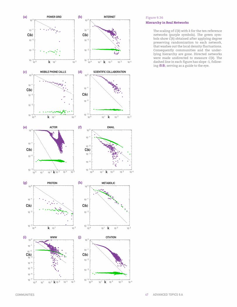
ADVANCED TOPICS 9.A47COMMUNITIES
10 -4
10 -3
10 -2
10 -1
10 0
10 0 10 1 10 2
POWER GRID
k
10 0 10 1 10 2k
C(k)
10 -5
10 -4
10 -3
10 -2
10 -1
10 0
C(k)
10 -4
10 -3
10 -2
10 -1
10 0
10 0 10 1 10 410 310 2
INTERNET
k
10 0 10 1 10 410 310 2k
10 0 10 1 10 410 310 2k
C(k)
10 -4
10 -3
10 -2
10 -1
10 0
10 0 10 1 10 2
MOBILE PHONE CALLS
k
C(k)
10 -7
10 -3
10 -4
10 -5
10 -6
10 -2
10 -1
10 0
C(k)
10 -4
10 -3
10 -2
10 -1
10 0
C(k)
10 -3
10 -2
10 -1
10 0
10 0 10 1 10 310 2
SCIENTIFIC COLLABORATION
k
10 0 10 1 10 310 2k
C(k)
10 -3
10 -2
10 -1
10 0
C(k)
10 -3
10 -2
10 -1
10 0
C(k)
10 -3
10 -2
10 -1
10 0
C(k)
ACTOR EMAIL
PROTEIN METABOLIC
WWW CITATION
10 0 10 1 10 4 10 510 310 2 k
10 0 10 1 10 4 10 510 310 2 k
(a)
(e)
(b)
(f)
(c)
(g)
(i)
(d)
(h)
(j)
Figure 9.36Hierarchy in Real Networks
The scaling of C(k) with k for the ten reference networks (purple symbols). The green sym-bols show C(k) obtained after applying degree preserving randomization to each network, that washes out the local density fluctuations. Consequently communities and the under-lying hierarchy are gone. Directed networks were made undirected to measure C(k). The dashed line in each figure has slope -1, follow-ing (9.8), serving as a guide to the eye.

ADVANCED TOPICS 9.BCOMMUNITIES 48
SECTION 9.11
In this section we derive the expressions (9.12) and (9.13), characterizing the modularity fuction and its changes.
Modularity as a Sum Over CommunitiesUsing (9.9) and (9.10) we can write the modularity of a full network as
, (9.51)
where Ci is the label of the community to which node i belongs to. As only node pairs that belong to the same community contribute to the sum in (9.51), we can rewrite the first term as a sum over communities,
(9.52)
where Lc is the number of links within community Cc. The factor 2 disap-pears because each link is counted twice in Aij.
In a similar fashion the second term of (9.51) becomes
, (9.53)
where kc is the total degree of the nodes in community Cc. Indeed, in the configuration model the probability that a stub connects to a randomly chosen stub is 1
2L, as in total we have 2L stubs in the network. Hence the
likelihood that our stub connects to a stub inside the module is kc
2L. By re-
peating this procedure for all kc stubs within the community Cc and adding 1/2 to avoid double counting, we obtain the last term of (9.53).
Combining (9.52) and (9.53) leads to (9.12).
M = 12L
N
∑i, j=1
(Aij −kikj
2L)δCi ,Cj
Ci ,Cj
12L
N
∑i, j=1
Aijδ =nc
∑c=1
12L ∑
i, j∈Cc
Aij =nc
∑c=1
Lc
L
12L ∑
i, j=1
kikj
2Lδ =
nN c
∑c=1
1(2L)2 ∑
i, j∈Cc
kikj =nc
∑c=1
kc2
4L2Ci ,Cj
ADVANCED TOPICS 9.BMODULARITY
COMMUNITIES

ADVANCED TOPICS 9.B49COMMUNITIES
Merging Two CommunitiesConsider communities A and B and denote with kA and kB the total de-
gree in these communities (equivalent with kc above). We wish to calculate the change in modularity after we merge these two communities. Using (9.12), this change can be written as
, (9.54)
where
, (9.55)
lAB is the number of direct links between the nodes of communities A and B, and
. (9.56)
After inserting (9.55) and (9.56) into (9.54), we obtain
(9.57)
which is (9.13).
ΔMAB = LAB
L−( kAB
2L )2
− LA
L− ( kA
2L )2+ LB
L− ( kB
2L )2
LAB= LA +LB + lAB
kAB = kA + kB
ΔMAB = lAB
L− kAkB
2L2

ADVANCED TOPICS 9.CCOMMUNITIES 50
SECTION 9.12
The algorithms discussed in this chapter were chosen to illustrate the fundamental ideas and concepts pertaining to community detection. Con-sequently they are not guaranteed to be neither the fastest nor the most ac-curate algorithms. Recently two algorithms, called the Louvain algorithm and Infomap have gained popularity, as their accuracy is comparable to the accuracy of the algorithms covered in this chapter but offer better scalability. Consequently we can use them to identify communities in very large networks.
There are many similarities between the two algorithms:
• They both aim to optimize a quality function Q . For the Louvain al-gorithm Q is modularity, M, and for Infomap Q is an entropy-based measure called the map equation or L.
• Both algorithms use the same optimization procedure.
Given these similarities, we discuss the algorithms together.
THE LOUVAIN ALGORITHMThe O(N2) computational complexity of the greedy algorithm can be
prohibitive for very large networks. A modularity optimization algorithm with better scalability was proposed by Blondel and collaborators [2]. The Louvain algorithm consists of two steps that are repeated iteratively (Figure
9.37):
Step IStart with a weighted network of N nodes, initially assigning each node to a different community. For each node i we evaluate the gain in mod-ularity if we place node i in the community of one of its neighbors j. We then move node i in the community for which the modularity gain is the largest, but only if this gain is positive. If no positive gain is found, i stays in its original community. This process is applied to all nodes until no further improvement can be achieved, completing Step I.
ADVANCED TOPICS 9.CFAST ALGORITHMS FOR COMMUNITY DETECTION
COMMUNITIES

ADVANCED TOPICS 9.C51COMMUNITIES
The modularity change ∆M obtained by moving an isolated node i into a community C can be calculated using
(9.58)
where ∑in is the sum of the weights of the links inside C (which is LC for an unweighted network); ∑tot is the sum of the link weights of all nodes in C; ki is the sum of the weights of the links incident to node i; ki,in is the sum of the weights of the links from i to nodes in C and W is the sum of the weights of all links in the network.
Note that ∆M is a special case of (9.13), which provides the change in modularity after merging communities A and B. In the current case B is an isolated node. We can use ∆M to determine the modularity change when i is removed from the community it belonged earlier. For this we calculate ∆M for merging i with the community C after we excluded i from it. The change after removing i is –∆M.
Step II We construct a new network whose nodes are the communities iden-tified during Step I. The weight of the link between two nodes is the sum of the weight of the links between the nodes in the correspond-ing communities. Links between nodes of the same community lead to weighted self-loops.
Once Step II is completed, we repeat Steps I - II, calling their combi-nation a pass (Figure 9.37). The number of communities decreases with each pass. The passes are repeated until there are no more changes and maximum modularity is attained.
ΔM = [ Σin + 2ki,in2W
− (Σtot + ki
2W )2
] − [ Σin
2W− (Σtot
2W )2
− ( ki
2W )2
]
15
2
212
44
4
9
5
1
1 1 1
7
3
3
14
14STEP I STEP II
1ST PASS
2ND PASS
16
811
1013
6
0
STEP I STEP II
15
2
12
4
9
7
3
13
65
1
14
8
11
10
0
2
44
1 1 1
3
14
16
243
26
2
44
1 1 1
3
14
16
∆M0,2 = 0 .023∆M0,3 = 0 .032∆M0,4 = 0 .026∆M0,5 = 0 .026
Figure 9.37The Louvain Algorithm
The main steps of the Louvain algorithm. Each pass consists of two distinct steps:
Step IModularity is optimized by local changes. We choose a node and calculate the change in modularity, (9.58), if the node joins the com-munity of its immediate neighbors. The figure shows the expected modularity change ∆Mo,i for node 0. Accordingly node 0 will join node 3, as the modularity change for this move is the largest, being ∆M0,3=0.032. This process is repeated for each node, the node colors corre-sponding to the resulting communities, con-cluding Step I.
Step II The communities obtained in Step I are aggre-gated, building a new network of communi-ties. Nodes belonging to the same community are merged into a single node, as shown on the top right. This process will generate self-loops, corresponding to links between nodes in the same community that are now merged into a single node.
The sum of Steps I & II are called a pass. The network obtained after each pass is processed again (Pass 2), until no further increase of modularity is possible. After [2].

ADVANCED TOPICS 9.C52COMMUNITIES
Computational Complexity The Louvain algorithm is more limited by storage demands than by computational time. The number of computations scale linearly with L for the most time consuming first pass. With subsequent passes over a decreasing number of nodes and links, the complexity of the algorithm is at most O(L). It therefore allows us to identify communities in net-works with millions of nodes.
INFOMAPIntroduced by Martin Rosvall and Carl T Bergstrom, Infomap exploits
data compression for community identification (Figure 9.38) [44-46]. It does it by optimizing a quality function for community detection in directed and weighted networks, called the map equation.
Consider a network partitioned into nc communities. We wish to encode in the most efficient fashion the trajectory of a random walker on this net-work. In other words, we want to describe the trojectory with the smallest number of symbols. The ideal code should take advantage of the fact that the random walker tends to get trapped into communities, staying there for a long time (Figure 9.38c).
To achieve this coding we assign:
• One code to each community (index codebook). For example the pur-ple community in Figure 9.38c is assigned the code 111.
• Codewords for each node within each community. For example thetop left node in (c) is assigned 001. Note that the same node code canbe reused in different communities.
• Exit codes that mark when the walker leavers a community, like 0001for the purple community in (c).
The goal, therefore, is to build a code that offers the shortest description of the random walk. Once we have this code, we can identify the network's community structure by reading the index codebook, which is uniquely as-
1111100
01011
1100
10000
0110
11011
001110111
10010100
111111 11010
10110
10101
11110
00011
00100000
1111101
10100
01010
1110
100010111
00010
0000
001
11
100
01
101
110011
00111
1010 100
010
00
10
011
11011
0010
010
1101
10
000111
1100
110 00010 0001
0 1011111 0001
110
10
0
111
1111100 1100 0110 11011 10000 11011 0110 0011 10111 1001 00111001 0100 0111 10001 1110 0111 10001 0111 1110 0000 1110 100010111 1110 0111 1110 1111101 1110 0000 10100 0000 1110 10001 01110100 10110 11010 10111 1001 0100 1001 10111 1001 0100 1001 01000011 0100 0011 0110 11011 0110 0011 0100 1001 10111 0011 01000111 10001 1110 10001 0111 0100 10110 111111 10110 10101 1111000011
111 0000 11 01 101 100 101 01 0001 0 110 011 00 110 00 111 1011 10111 000 10 111 000 111 10 011 10 000 111 10 111 10 0010 10 011 010011 10 000 111 0001 0 111 010 100 011 00 111 00 011 00 111 00 111110 111 110 1011 111 01 101 01 0001 0 110 111 00 011 110 111 101110 111 000 10 000 111 0001 0 111 010 1010 010 1011 110 00 10 011
111 0 110 011 00 110 00 111 1011 10111 000 10 111 000 111 10 011 10 000 111 10 111 10 0010 10 011 010011 10 000 111 0001 0 111 010 100 011 00 111 00 011 00 111 00 111110 111 110 1011 111 0 110 111 00 011 110 111 101110 111 000 10 000 111 0001 0 111 010 1010 010 1011 110 00 10 011
1111100
01011
1100
10000
0110
11011
001110111
10010100
111111 11010
10110
10101
11110
00011
00100000
1111101
10100
01010
1110
100010111
00010
0000
001
11
100
01
101
110011
00111
1010 100
010
00
10
011
11011
0010
010
1101
10
000111
1100
110 00010 0001
0 1011111 0001
110
10
0
111
1111100 1100 0110 11011 10000 11011 0110 0011 10111 1001 00111001 0100 0111 10001 1110 0111 10001 0111 1110 0000 1110 100010111 1110 0111 1110 1111101 1110 0000 10100 0000 1110 10001 01110100 10110 11010 10111 1001 0100 1001 10111 1001 0100 1001 01000011 0100 0011 0110 11011 0110 0011 0100 1001 10111 0011 01000111 10001 1110 10001 0111 0100 10110 111111 10110 10101 1111000011
111 0000 11 01 101 100 101 01 0001 0 110 011 00 110 00 111 1011 10111 000 10 111 000 111 10 011 10 000 111 10 111 10 0010 10 011 010011 10 000 111 0001 0 111 010 100 011 00 111 00 011 00 111 00 111110 111 110 1011 111 01 101 01 0001 0 110 111 00 011 110 111 101110 111 000 10 000 111 0001 0 111 010 1010 010 1011 110 00 10 011
111 0000 11 01 101 100 101 01 0001 0 110 011 00 110 00 111 1011 10111 000 10 111 000 111 10 011 10 000 111 10 111 10 0010 10 011 010011 10 000 111 0001 0 111 010 100 011 00 111 00 011 00 111 00 111110 111 110 1011 111 01 101 01 0001 0 110 111 00 011 110 111 101110 111 000 10 000 111 0001 0 111 010 1010 010 1011 110 00 10 011
(a) (b) (c) (d)
Figure 9.38From Data Compression to Communities
Infomap detect communities by compressing the movement of a random walker on a net-work.
(a) The orange line shows the trajectory of a random walker on a small network. We want to describe this trajectory with a minimal number of symbols, which we can achieve by assigning repeatedly used structures (communities) short and unique names.
(b) We start by giving a unique name to each node. This is derived using a Huffman coding, a data compression algorithm that assigns each node a code using the esti-mated probability that the random walk visits that node. The 314 bits under the network describe the sample trajectory of the random walker shown in (a), starting with 1111100 for the first node of the walk in the upper left corner, 1100 for the sec-ond node, etc., and ending with 00011 for the last node on the walk in the lower right corner.
(c) The figure shows a two-level encoding of the random walk, in which each commu-nity receives a unique name, but the name of nodes within communities are reused. This code yields on average a 32% shorter coding. The codes naming the communi-ties and the codes used to indicate an exit from each community are shown to the left and the right of the arrows under the network, respectively. Using this code, we can describe the walk in (a) by the 243 bits shown under the network in (c). The first three bits 111 indicate that the walk begins in the red community, the code 0000 spec-ifies the first node of the walk, etc.
( ) By reporting only the community names, and not the locations of each node within the communities, we obtain an efficient coarse graining of the network, which cor-responds to its community structure.

ADVANCED TOPICS 9.C53COMMUNITIES
signed to each community (Figure 9.38c).
The optimal code is obtained by finding the minimum of the map equa-tion
. (9.59)
In a nutshell, the first term of (9.59) gives the average number of bits neces-sary to describe the movement between communities where q is the prob-ability that the random walker switches communities during a given step.
The second term gives the average number of bits necessary to describe movement within communities. Here H(Pc) is the entropy of within-com-munity movements — including an “exit code” to capture the departure from a community i.
The specific terms of the maps equation and their calculation in terms of the probabilities capturing the movement of a random walker on a net-work, is somewhat involved. They are described in detail in Ref [44-46]. Online Resource 9.3 offers an interactive tool to illustrate the mechanism be-hind (9.59) and its use.
At the end L serves as a quality function, that takes up a specific value for a particular partition of the network into communities. To find the best partition, we must minimize L over all possible partitions. The popular im-plementation of this optimization procedure follows Steps I and II of the Louvain algorithm: We assign each node to a separate community, and we systematically join neighboring nodes into modules if the move decreases L. After each move L is updated using (9.59). The obtained communities are joined into supercommunities, finishing a pass, after which the algorithm is restarted on the new, reduced network.
Computational Complexity The computational complexity of Infomap is determined by the pro-
cedure used to minimize the map equation L. If we use the Louvain pro-cedure, the computational complexity is the same as that of the Louvain algorithm, i.e. at most O(LlogL) or O(NlogN) for a sparse graph.
In summary, the Louvain algorithm and Infomap offer tools for fast community identification. Their accuracy across benchmarks is compara-ble to the accuracy of the algorithms discussed throughout this chapter (Figure 9.28).
L= qH(Q) +nc
∑c =1
p↻cH(Pc)
>Online Resource 9.3
Map Equation for Infomap
For a dynamic visualization of the mechanism behind the map equation, see http://www.tp.umu. se/~rosvall/livemod/mapequation/.
>

ADVANCED TOPICS 9.DCOMMUNITIES 54
SECTION 9.13
In this section we derive the percolation threshold (9.20) for clique percola-tion on a random network and discuss the main steps of the CFinder algo-rithm (Figure 9.39).
When we roll a k-clique to an adjacent k-clique by relocating one of its nodes, the expectation value of the number of adjacent k-cliques for the template to roll further should equal exactly one at the percolation thresh-old (Figure 9.20). Indeed, a smaller than one expectation value will result in a premature end of the k-clique percolation clusters, because starting from any k-clique, the rolling would quickly come to a halt. Consequently the size of the clusters would decay exponentially. A larger than one expecta-tion value, on the other hand, allows the clique community to grow indefi-nitely, guaranteeing that we have a giant cluster in the system.
The above expectation value is provided by
, (9.63)
where the term (k–1) counts the number of nodes of the template that can be selected for the next relocation; the term (N-k–1)k–1 counts the number of potential destinations for this relocation, out of which only the fraction pk–1 is acceptable, because each of the new k–1 edges (associated with the relocation) must exist in order to obtain a new k-clique. For large N, (9.63) simplifies to
(k–1)Npck–1 = 1 ,
which leads to (9.16).
(k − 1)(N − k − 1)k−1
ADVANCED TOPICS 9.DTHRESHOLD FOR CLIQUE PERCOLATION
COMMUNITIES

ADVANCED TOPICS 9.DCOMMUNITIES 55
1 2 3 4 51 0 1 0 0 02 1 0 0 0 03 0 0 0 1 04 0 0 1 0 15 0 0 0 1 0
O=
1
23 4 5
1 23
45
(a)
(b)
(c)
Figure 9.39CFinder algorithm
The main steps of the CFinder algorithm.
(a) Starting from the network shown in the figure, our goal is to identify all cliques. All five k=3 cliques present in the network are highlighted.
(b) The overlap matrix O of the k=3 cliques. This matrix is viewed as an adjacency matrix of a network whose nodes are the cliques of the original network. The ma-trix indicates that we have two connect-ed components, one consisting of cliques (1,2) and the other of cliques (3, 4, 5). The connected components of this network map into the communities of the original network.
(c) The two clique communities predicted by the adjacency matrix.
(d) The two clique communities shown in (c), mapped on the original network.
(d)

BIBLIOGRAPHYCOMMUNITIES 56
[1] B. Droitcour. Young Incorporated Artists. Art in America, 92-97, April 2014.
[2] V. D. Blondel, J.-L. Guillaume, R. Lambiotte, and E. Lefebvre. Fast un-folding of communities in large networks. J. Stat. Mech., 2008.
[3] G.C. Homans. The Human Groups. Harcourt, Brace & Co, New York, 1950.
[4] S.A. Rice. The identification of blocs in small political bodies. Am. Polit. Sci. Rev., 21:619–627, 1927.
[5] R.D. Luce and A.D. Perry. A method of matrix analysis of group struc-ture. Psychometrika, 14:95–116, 1949.
[6] R.S. Weiss and E. Jacobson. A method for the analysis of the struc-ture of complex organizations. Am. Sociol. Rev., 20:661–668, 1955.
[7] W.W. Zachary. An information flow model for conflict and fission in small groups. J. Anthropol. Res., 33:452–473, 1977.
[8] L. Donetti and M.A. Muñoz. Detecting network communities: a new systematic and efficient algorithm. J. Stat. Mech., P10012, 2004.
[9] M. Girvan and M.E.J. Newman. Community structure in social and biological networks. PNAS, 99:7821–7826, 2002.
[10] L.H. Hartwell, J.J. Hopfield, and A.W. Murray. From molecular to modular cell biology. Nature, 402:C47–C52, 1999.
[11] E. Ravasz, A. L. Somera, D. A. Mongru, Z. N. Oltvai, and A.-L. Barabási. Hierarchical organization of modularity in metabolic networks. Science, 297:1551-1555, 2002.
[12] K.-I. Goh, M. E. Cusick, D. Valle, B. Childs, M. Vidal, and A.-L. Barabá-si. The human disease network. PNAS, 104:8685-8690, 2007.
SECTION 9.14
BIBLIOGRAPHY
COMMUNITIES
57 BIBLIOGRAPHY
[13] J. Menche, A.Sharma, M. Kitsak, S. Ghiassian, M. Vidal, J. Loscalzo, A.-L. Barabási. Oncovering disease-disease relationships through the hu-man interactome. 2014.
[14] A.-L. Barabási, N. Gulbahce, and J. Loscalzo. Network medicine: a network-based approach to human disease. Nature Review Genetics, 12:56-68, 2011.
[15] G. W. Flake, S. Lawrence, and C.L. Giles. Efficient identification of web communities. Proceedings of the sixth ACM SIGKDD international conference on Knowledge discovery and data mining, 150-160, 2000.
[16] F. Radicchi, C. Castellano, F. Cecconi, V. Loreto, and D. Parisi. Defin-ing and identifying communities in networks. PNAS, 101:2658–2663, 2004.
[17] A.B. Kahng, J. Lienig, I.L. Markov, and J. Hu. VLSI Physical Design: From Graph Partitioning to Timing Closure. Springer, 2011.
[18] B.W. Kernighan and S. Lin. An efficient heuristic procedure for par-titioning graphs. Bell Systems Technical Journal, 49:291–307, 1970.
[19] G.E. Andrews. The Theory of Partitions. Addison-Wesley, Boston, USA, 1976.
[20] L. Lovász. Combinatorial Problems and Exercises. North-Holland, Amsterdam, The Netherlands, 1993.
[21] G. Pólya and G. Szegő. Problems and Theorems in Analysis I. Spring-er-Verlag, Berlin, Germany, 1998.
[22] V. H. Moll. Numbers and Functions: From a classical-experimental mathematician’s point of view. American Mathematical Society, 2012.
[23] M.E.J. Newman and M. Girvan. Finding and evaluating community structure in networks. Physical Review E, 69:026113, 2004.
[24] M.E.J. Newman. A measure of betweenness centrality based on random walks. Social Networks, 27:39–54, 2005.
[25] U. Brandes. A faster algorithm for betweenness centrality. J. Math. Sociol., 25:163–177, 2001.
[26] T. Zhou, J.-G. Liu, and B.-H. Wang. Notes on the calculation of node betweenness. Chinese Physics Letters, 23:2327–2329, 2006.
[27] E. Ravasz and A.-L. Barabasi. Hierarchical organization in complex networks. Physical Review E, 67:026112, 2003.
[28] S. N. Dorogovtsev, A. V. Goltsev, and J. F. F. Mendes. Pseudofractal scale-free web. Physical Review E, 65:066122, 2002.
[29] E. Mones, L. Vicsek, and T. Vicsek. Hierarchy Measure for Complex Networks. PLoS ONE, 7:e33799, 2012.
COMMUNITIES

58 BIBLIOGRAPHY
[30] A. Clauset, C. Moore, and M. E. J. Newman. Hierarchical structure and the prediction of missing links in networks. Nature, 453:98-101, 2008.
[31] L. Danon, A. Díaz-Guilera, J. Duch, and A. Arenas. Comparing com-munity structure identification. Journal of Statistical Mechanics, P09008, 2005.
[32] S. Fortunato and M. Barthélemy. Resolution limit in community de-tection. PNAS, 104:36–41, 2007.
[33] M.E.J. Newman. Fast algorithm for detecting community structure in networks. Physical Review E, 69:066133, 2004.
[34] S. Fortunato and M. Barthélemy. Resolution limit in community de-tection. PNAS, 104:36–41, 2007.
[35] A. Clauset, M.E.J. Newman, and C. Moore. Finding community structure in very large networks. Physical Review E, 70:066111, 2004.
[36] G. Palla, I. Derényi, I. Farkas, and T. Vicsek. Uncovering the over-lapping community structure of complex networks in nature and society. Nature, 435:814, 2005.
[37] R. Guimerà, L. Danon, A. Díaz-Guilera, F. Giralt, and A. Arenas. Self-similar community structure in a network of human interactions. Physical Review E, 68:065103, 2003.
[38] L. Danon, A. Díaz-Guilera, J. Duch, and A. Arenas. Comparing com-munity structure identification. J. Stat. Mech., P09008, 2005.
[39] J. Ruan and W. Zhang. Identifying network communities with a high resolution. Physical Review E 77: 016104, 2008.
[40] B. H. Good, Y.-A. de Montjoye, and A. Clauset. The performance of modularity maximization in practical contexts. Physical Review E, 81:046106, 2010.
[41] R. Guimerá, M. Sales-Pardo, and L.A.N. Amaral. Modularity from fluctuations in random graphs and complex networks. Physical Review E, 70:025101, 2004.
[42] J. Reichardt and S. Bornholdt. Partitioning and modularity of graphs with arbitrary degree distribution. Physical Review E, 76:015102, 2007.
[43] J. Reichardt and S. Bornholdt. When are networks truly modular? Physica D, 224:20–26, 2006.
[44] M. Rosvall and C.T. Bergstrom. Maps of random walks on complex networks reveal community structure. PNAS, 105:1118, 2008.
[45] M. Rosvall, D. Axelsson, and C.T. Bergstrom. The map equation. Eur. Phys. J. Special Topics, 178:13, 2009.
COMMUNITIES

BIBLIOGRAPHY59COMMUNITIES
[46] M. Rosvall and C.T. Bergstrom. Mapping change in large networks. PLoS ONE, 5:e8694, 2010.
[47] A. Perey. Oksapmin Society and World View. Dissertation for De-gree of Doctor of Philosophy. Columbia University, 1973.
[48] I. Derényi, G. Palla, and T. Vicsek. Clique percolation in random net-works. Physical Review Letters, 94:160202, 2005.
[49] J.M. Kumpula, M. Kivelä, K. Kaski, and J. Saramäki. A sequential al-gorithm for fast clique percolation. Physical Review E, 78:026109, 2008.
[50] G. Palla, A.-L. Barabási, and T. Vicsek. Quantifying social group evo-lution. Nature, 446:664-667, 2007.
[51] Y.-Y. Ahn, J. P. Bagrow, and S. Lehmann. Link communities reveal multiscale complexity in networks. Nature, 466:761-764, 2010.
[52] T.S. Evans and R. Lambiotte. Line graphs, link partitions, and over-lapping communities. Physical Review E, 80:016105, 2009.
[53] M. Chen, K. Kuzmin, and B.K. Szymanski. Community Detection via Maximization of Modularity and Its Variants. IEEE Trans. Computational Social Systems, 1:46-65, 2014.
[54] I. Farkas, D. Ábel, G. Palla, and T. Vicsek. Weighted network mod-ules. New J. Phys., 9:180, 2007.
[55] S. Lehmann, M. Schwartz, and L.K. Hansen. Biclique communities. Physical Review E, 78:016108, 2008.
[56] N. Du, B. Wang, B. Wu, and Y. Wang. Overlapping community de-tection in bipartite networks. IEEE/WIC/ACM International Conference on Web Intelligence and Intelligent Agent Technology, IEEE Computer Soci-ety, Los Alamitos, CA, USA: 176–179, 2008.
[57] A. Condon and R.M. Karp. Algorithms for graph partitioning on the planted partition model. Random Struct. Algor., 18:116–140, 2001.
[58] A. Lancichinetti, S. Fortunato, and F. Radicchi. Benchmark graphs for testing community detection algorithms. Physical Review E, 78:046110, 2008.
[59] A. Lancichinetti, S. Fortunato, and J. Kertész. Detecting the over-lapping and hierarchical community structure of complex networks. New Journal of Physics, 11:033015, 2009.
[60] S. Fortunato. Community detection in graphs. Physics Reports, 486:75–174, 2010.
[61] D. Hric, R.K. Darst, and S. Fortunato. Community detection in networks: structural clusters versus ground truth. Physical Review E, 90:062805, 2014.

BIBLIOGRAPHY60COMMUNITIES
[62] M. S. Granovetter. The Strength of Weak Ties. The American Journal of Sociology, 78:1360–1380, 1973.
[63] J.-P. Onnela, J. Saramäki, J. Hyvönen, G. Szabó, D. Lazer, K. Kaski, J. Kertész, and A.-L. Barabási. Structure and tie strengths in mobile commu-nication networks. PNAS, 104:7332, 2007.
[64] K.-I. Goh, B. Kahng, and D. Kim. Universal Behavior of Load Distri-bution in Scale-Free Networks. Physical Review Letters, 87:278701, 2001.
[65] A. Maritan, F. Colaiori, A. Flammini, M. Cieplak, and J.R. Banavar. Universality Classes of Optimal Channel Networks. Science, 272:984 –986, 1996.
[66] L.C. Freeman. A set of measures of centrality based upon between-ness. Sociometry, 40:35–41, 1977.
[67] J. Hopcroft, O. Khan, B. Kulis, and B. Selman. Tracking evolving communities in large linked networks. PNAS, 101:5249–5253, 2004.
[68] S. Asur, S. Parthasarathy, and D. Ucar. An event-based frame-work for characterizing the evolutionary behavior of interaction graphs. KDD ’07: Proceedings of the 13th ACM SIGKDD International Conference on Knowledge Discovery and Data Mining, ACM, New York, NY, USA, pp. 913–921, 2007.
[69] D.J. Fenn, M.A. Porter, M. McDonald, S. Williams, N.F. Johnson, and N.S. Jones. Dynamic communities in multichannel data: An application to the foreign exchange market during the 2007–2008 credit crisis. Chaos, 19:033119, 2009.
[70] D. Chakrabarti, R. Kumar, and A. Tomkins. Evolutionary cluster-ing, in: KDD ’06: Proceedings of the 12th ACM SIGKDD International Con-ference on Knowledge Discovery and Data Mining, ACM, New York, NY, USA, pp. 554–560, 2006.
[71] Y. Chi, X. Song, D. Zhou, K. Hino, and B.L. Tseng. Evolutionary spec-tral clustering by incorporating temporal smoothness. KDD ’07: Proceed-ings of the 13th ACM SIGKDD International Conference on Knowledge Dis-covery and Data Mining, ACM, New York, NY, USA, pp. 153–162, 2007.
[72] Y.-R. Lin, Y. Chi, S. Zhu, H. Sundaram, and B.L. Tseng. Facetnet: a framework for analyzing communities and their evolutions in dynamic networks. in: WWW ’08: Proceedings of the 17th International Conference on the World Wide Web, ACM, New York, NY, USA, pp. 685–694, 2008.
[73] L. Backstrom, D. Huttenlocher, J. Kleinberg, and X. Lan. Group formation in large social networks: membership, growth, and evolution. KDD ’06: Proceedings of the 12th ACM SIGKDD International Conference on Knowledge Discovery and Data Mining, ACM, New York, NY, USA, pp. 44–54, 2006.

BIBLIOGRAPHY61COMMUNITIES
[74] M. E. J. Newman and J. Park. Why social networks are different from other types of networks. Physical Review E, 03G122, 2003.
[75] B. Krishnamurthy and J. Wang. On network-aware clustering of web clients. SIGCOMM Comput. Commun. Rev., 30:97–110, 2000.
[76] K.P. Reddy, M. Kitsuregawa, P. Sreekanth, and S.S. Rao. A graph based approach to extract a neighborhood customer community for collab-orative filtering. DNIS ’02: Proceedings of the Second International Work-shop on Databases in Networked Information Systems, Springer-Verlag, London, UK, pp. 188–200, 2002.
[77] R. Agrawal and H.V. Jagadish. Algorithms for searching massive graphs. Knowl. Data Eng., 6:225–238, 1994.
[78] A.Y. Wu, M. Garland, and J. Han. Mining scale-free networks using geodesic clustering. KDD ’04: Proceedings of the Tenth ACM SIGKDD Inter-national Conference on Knowledge Discovery and Data Mining, ACM Press, New York, NY, USA, 2004, pp. 719–724, 2004.