alberto abad, antonio elipe grupo de mec´anica espacial...
TRANSCRIPT
Analytical Model for Lunar Orbiter
Alberto Abad, Antonio Elipe
Grupo de Mecanica Espacial, University of Zaragoza, Spain
Juan Felix San-Juan, Montserrat San-Martın
Dpt. Maths & Computation, University of La Rioja, Spain
A. Abad, A. Elipe, J.F. San-Juan & M. San-Martın CADE 2007. Turku. 2
Moon orbiter
• Theoretical interest:
– Normal forms in perturbed Hamiltonians
– Periodic orbits
– Bifurcations, . . .
• Practical interest:
– Science missions to the Moon, Jovian satellites, . . .

A. Abad, A. Elipe, J.F. San-Juan & M. San-Martın CADE 2007. Turku. 3
Frozen orbits
Definition: Those whose average e and I are constant.
They are the equilibria of the zonal problem, once short period terms
are removed. That is, mean orbits with fixed e, I and ω.
Example: Critical inclination in the main problem
Interest: avoiding maneuvers
repeated elevation at each pass
maintaining relative configuration
. . .

A. Abad, A. Elipe, J.F. San-Juan & M. San-Martın CADE 2007. Turku. 4
How are they determined?
• Find equilibria in the Gauss (Lagrange) equations
• Normal forms
• Continuation of families of periodic orbits
• . . .
A. Abad, A. Elipe, J.F. San-Juan & M. San-Martın CADE 2007. Turku. 5
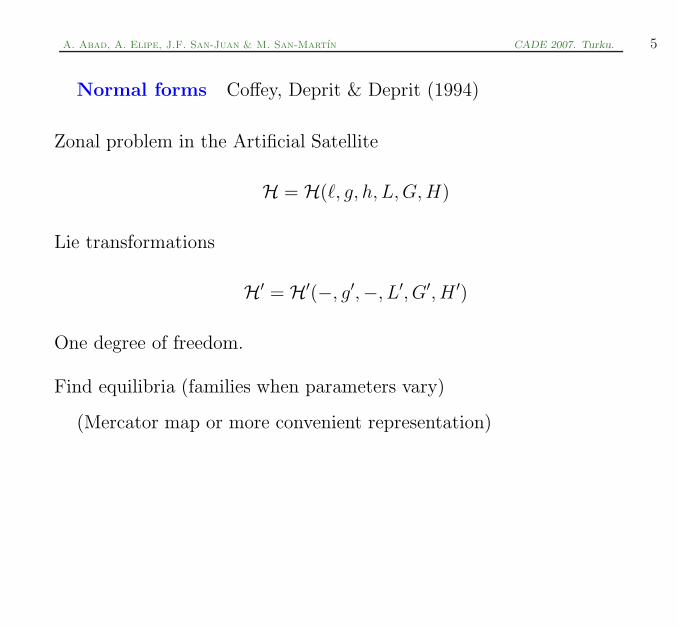
Normal forms Coffey, Deprit & Deprit (1994)
Zonal problem in the Artificial Satellite
H = H(ℓ, g, h, L, G, H)
Lie transformations
H′ = H′(−, g′,−, L′, G′, H ′)
One degree of freedom.
Find equilibria (families when parameters vary)
(Mercator map or more convenient representation)

A. Abad, A. Elipe, J.F. San-Juan & M. San-Martın CADE 2007. Turku. 6
Families of periodic orbits
Broucke; Deprit, Elipe & Lara, . . .
Consider the system
x = 2Ay + Wx,
y = −2Ay + Wy,
with the integral
C = 2W − (x2 + y2)
and
A = A(x, y; σ), W = W (x, y; σ). σ a parameter
A. Abad, A. Elipe, J.F. San-Juan & M. San-Martın CADE 2007. Turku. 7
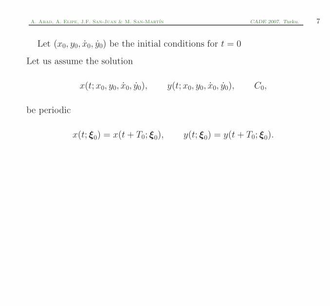
Let (x0, y0, x0, y0) be the initial conditions for t = 0
Let us assume the solution
x(t; x0, y0, x0, y0), y(t; x0, y0, x0, y0), C0,
be periodic
x(t; ξ0) = x(t + T0; ξ0), y(t; ξ0) = y(t + T0; ξ0).
A. Abad, A. Elipe, J.F. San-Juan & M. San-Martın CADE 2007. Turku. 8
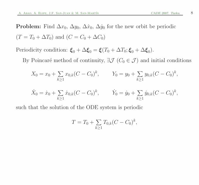
Problem: Find ∆x0, ∆y0, ∆x0, ∆y0 for the new orbit be periodic
(T = T0 + ∆T0) and (C = C0 + ∆C0)
Periodicity condition: ξ0 + ∆ξ0 = ξ(T0 + ∆T0; ξ0 + ∆ξ0).
By Poincare method of continuity, ∃J (C0 ∈ J ) and initial conditions
X0 = x0 +∑
k≥1
x0,k(C − C0)k, Y0 = y0 +
∑
k≥1
y0,k(C − C0)k,
X0 = x0 +∑
k≥1
x0,k(C − C0)k, Y0 = y0 +
∑
k≥1
y0,k(C − C0)k,
such that the solution of the ODE system is periodic
T = T0 +∑
k≥1
T0,k(C − C0)k,
A. Abad, A. Elipe, J.F. San-Juan & M. San-Martın CADE 2007. Turku. 9
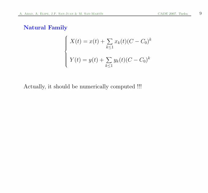
Natural Family
X(t) = x(t) +∑
k≤1
xk(t)(C − C0)k
Y (t) = y(t) +∑
k≤1
yk(t)(C − C0)k
Actually, it should be numerically computed !!!
A. Abad, A. Elipe, J.F. San-Juan & M. San-Martın CADE 2007. Turku. 10
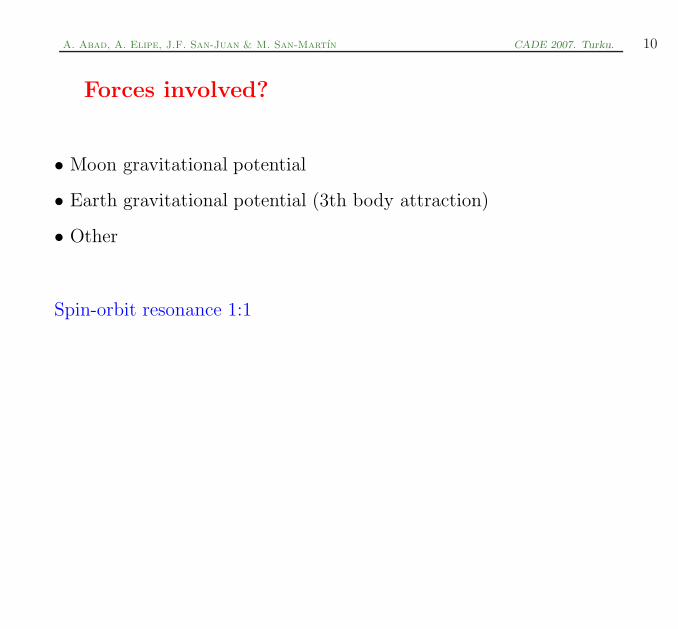
Forces involved?
• Moon gravitational potential
• Earth gravitational potential (3th body attraction)
• Other
Spin-orbit resonance 1:1
A. Abad, A. Elipe, J.F. San-Juan & M. San-Martın CADE 2007. Turku. 11
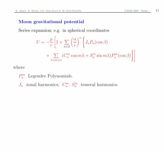
Moon gravitational potential
Series expansion; e.g. in spherical coordinates
U = −µ
r
1 +
∑
n≥2
(α
r
)nJnPn(cosβ)
+∑
1≤m≤n
(Cmn cos mλ + Sm
n sin mλ)Pmn (cosβ)
where
Pmn Legendre Polynomials.
Jn zonal harmonics; Cmn , Sm
n tesseral harmonics.
A. Abad, A. Elipe, J.F. San-Juan & M. San-Martın CADE 2007. Turku. 12
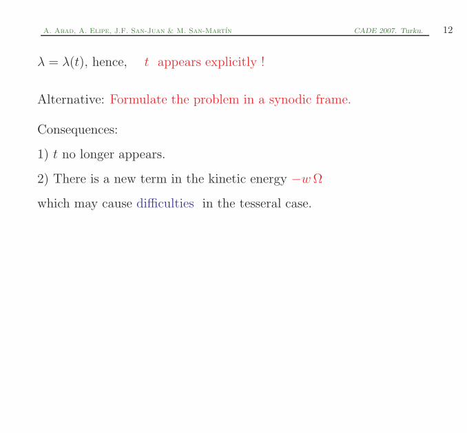
λ = λ(t), hence, t appears explicitly !
Alternative: Formulate the problem in a synodic frame.
Consequences:
1) t no longer appears.
2) There is a new term in the kinetic energy −w Ω
which may cause difficulties in the tesseral case.
A. Abad, A. Elipe, J.F. San-Juan & M. San-Martın CADE 2007. Turku. 13
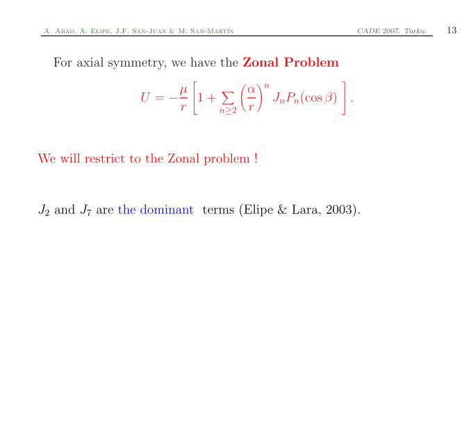
For axial symmetry, we have the Zonal Problem
U = −µ
r
1 +
∑
n≥2
(α
r
)n
JnPn(cosβ)
.
We will restrict to the Zonal problem !
J2 and J7 are the dominant terms (Elipe & Lara, 2003).
A. Abad, A. Elipe, J.F. San-Juan & M. San-Martın CADE 2007. Turku. 14
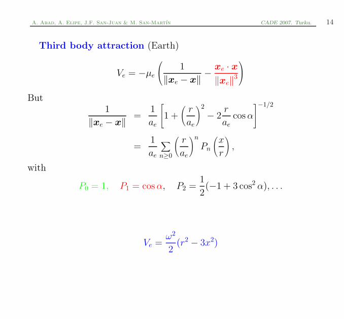
Third body attraction (Earth)
Ve = −µe
1
‖xe − x‖−
xe · x
‖xe‖3
But1
‖xe − x‖=
1
ae
1 +
(r
ae
)2
− 2r
aecos α
−1/2
=1
ae
∑
n≥0
(r
ae
)n
Pn
(x
r
),
with
P0 = 1, P1 = cos α, P2 =1
2(−1 + 3 cos2 α), . . .
Ve =ω2
2(r2 − 3x2)
A. Abad, A. Elipe, J.F. San-Juan & M. San-Martın CADE 2007. Turku. 15
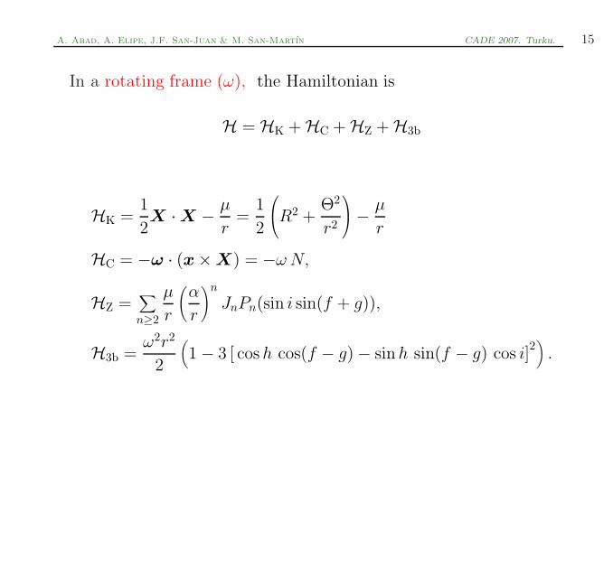
In a rotating frame (ω), the Hamiltonian is
H = HK + HC + HZ + H3b
HK =1
2X · X −
µ
r=
1
2
R2 +
Θ2
r2
−
µ
r
HC = −ω · (x × X) = −ω N,
HZ =∑
n≥2
µ
r
(α
r
)n
JnPn(sin i sin(f + g)),
H3b =ω2r2
2
(1 − 3 [ cos h cos(f − g) − sinh sin(f − g) cos i]
2)
.
A. Abad, A. Elipe, J.F. San-Juan & M. San-Martın CADE 2007. Turku. 16
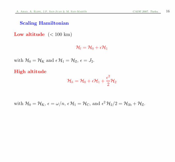
Scaling Hamiltonian
Low altitude (< 100 km)
Hl = H0 + ǫH1
with H0 = HK and ǫH1 = HZ, ǫ = J2.
High altitude
Hh = H0 + ǫH1 +ǫ2
2H2
with H0 = HK, ǫ = ω/n, ǫH1 = HC, and ǫ2 H2/2 = H3b + HZ.
A. Abad, A. Elipe, J.F. San-Juan & M. San-Martın CADE 2007. Turku. 17
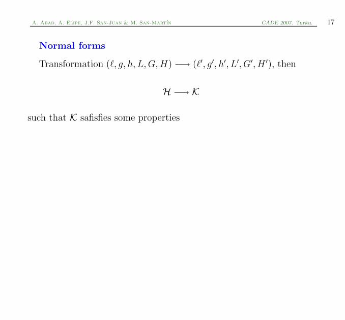
Normal forms
Transformation (ℓ, g, h, L, G, H) −→ (ℓ′, g′, h′, L′, G′, H ′), then
H −→ K
such that K safisfies some properties
A. Abad, A. Elipe, J.F. San-Juan & M. San-Martın CADE 2007. Turku. 18
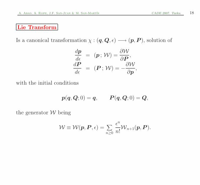
Lie Transform
Is a canonical transformation χ : (q, Q, ǫ) −→ (p, P ), solution of
dp
dǫ= (p ; W) =
∂W
∂P,
dP
dǫ= (P ; W) = −
∂W
∂p,
with the initial conditions
p(q, Q; 0) = q, P (q, Q; 0) = Q,
the generator W being
W ≡ W(p, P , ǫ) =∑
n≥0
ǫn
n!Wn+1(p, P ).
A. Abad, A. Elipe, J.F. San-Juan & M. San-Martın CADE 2007. Turku. 19
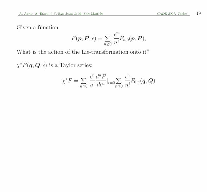
Given a function
F (p, P , ǫ) =∑
n≥0
ǫn
n!Fn,0(p, P ),
What is the action of the Lie-transformation onto it?
χ∗F (q, Q, ǫ) is a Taylor series:
χ∗F =∑
n≥0
ǫn
n!
dnF
dǫn|ǫ=0
∑
n≥0
ǫn
n!F0,n(q, Q)
A. Abad, A. Elipe, J.F. San-Juan & M. San-Martın CADE 2007. Turku. 20
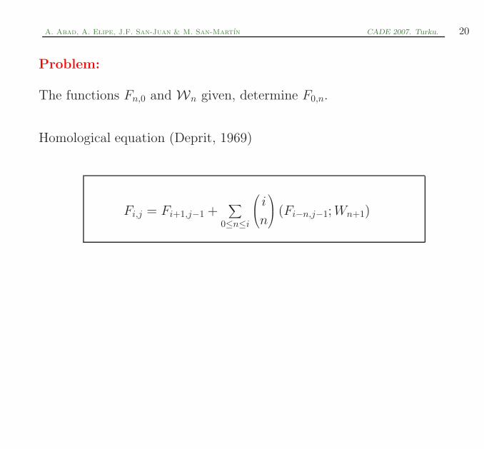
Problem:
The functions Fn,0 and Wn given, determine F0,n.
Homological equation (Deprit, 1969)
Fi,j = Fi+1,j−1 +∑
0≤n≤i
i
n
(Fi−n,j−1; Wn+1)
A. Abad, A. Elipe, J.F. San-Juan & M. San-Martın CADE 2007. Turku. 21
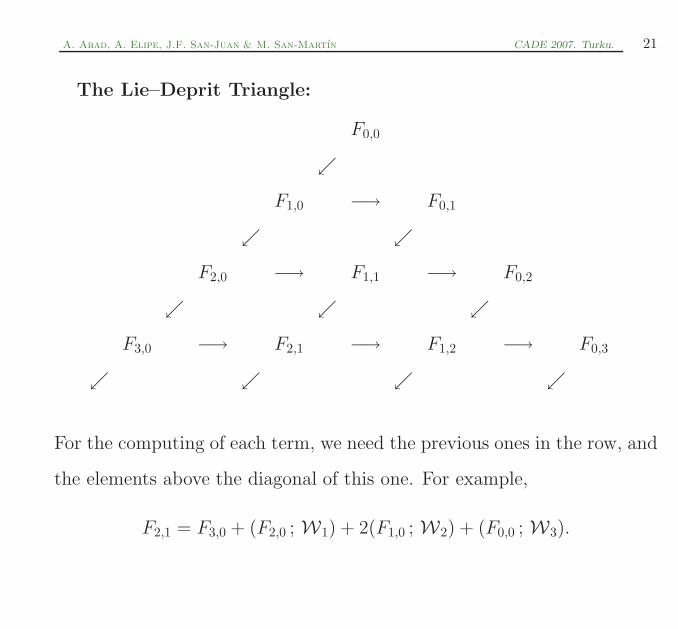
The Lie–Deprit Triangle:
F0,0
ւ
F1,0 −→ F0,1
ւ ւ
F2,0 −→ F1,1 −→ F0,2
ւ ւ ւ
F3,0 −→ F2,1 −→ F1,2 −→ F0,3
ւ ւ ւ ւ
For the computing of each term, we need the previous ones in the row, and
the elements above the diagonal of this one. For example,
F2,1 = F3,0 + (F2,0 ; W1) + 2(F1,0 ; W2) + (F0,0 ; W3).
A. Abad, A. Elipe, J.F. San-Juan & M. San-Martın CADE 2007. Turku. 22
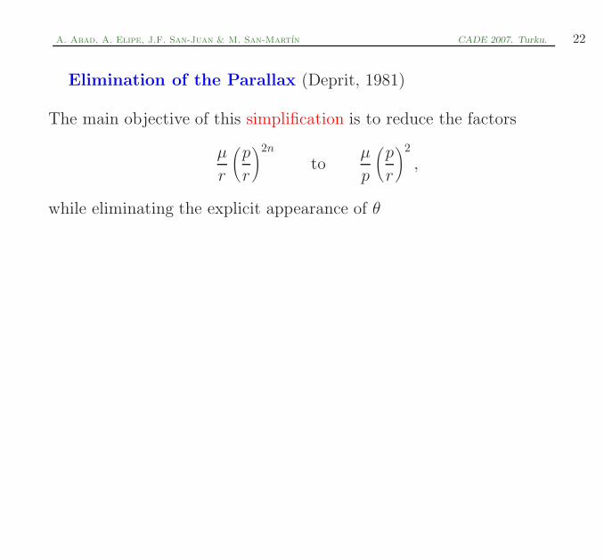
Elimination of the Parallax (Deprit, 1981)
The main objective of this simplification is to reduce the factors
µ
r
(p
r
)2n
toµ
p
(p
r
)2
,
while eliminating the explicit appearance of θ
A. Abad, A. Elipe, J.F. San-Juan & M. San-Martın CADE 2007. Turku. 23
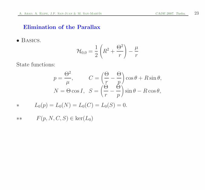
Elimination of the Parallax
• Basics.
H0,0 =1
2
R2 +
Θ2
r
−
µ
r
State functions:
p =Θ2
µ, C =
(Θ
r−
Θ
p
)cos θ + R sin θ,
N = Θ cos I, S =
(Θ
r−
Θ
p
)sin θ − R cos θ,
∗ L0(p) = L0(N) = L0(C) = L0(S) = 0.
∗∗ F (p, N, C, S) ∈ ker(L0)
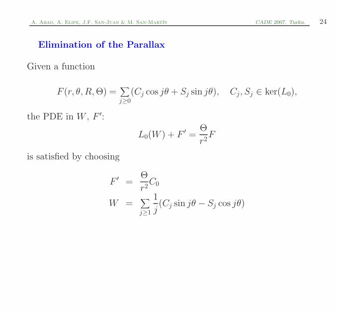
A. Abad, A. Elipe, J.F. San-Juan & M. San-Martın CADE 2007. Turku. 24
Elimination of the Parallax
Given a function
F (r, θ, R, Θ) =∑
j≥0
(Cj cos jθ + Sj sin jθ), Cj, Sj ∈ ker(L0),
the PDE in W , F ′:
L0(W ) + F ′ =Θ
r2F
is satisfied by choosing
F ′ =Θ
r2C0
W =∑
j≥1
1
j(Cj sin jθ − Sj cos jθ)
A. Abad, A. Elipe, J.F. San-Juan & M. San-Martın CADE 2007. Turku. 25
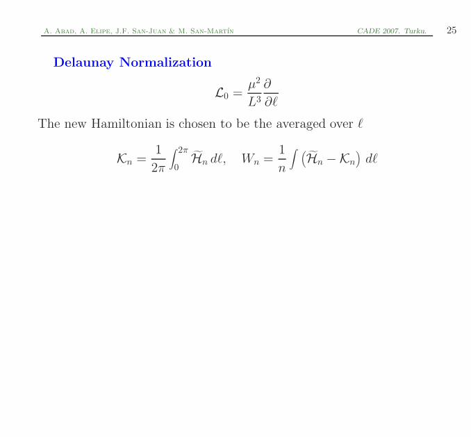
Delaunay Normalization
L0 =µ2
L3
∂
∂ℓ
The new Hamiltonian is chosen to be the averaged over ℓ
Kn =1
2π
∫ 2π
0Hn dℓ, Wn =
1
n
∫ (Hn −Kn
)dℓ
A. Abad, A. Elipe, J.F. San-Juan & M. San-Martın CADE 2007. Turku. 26
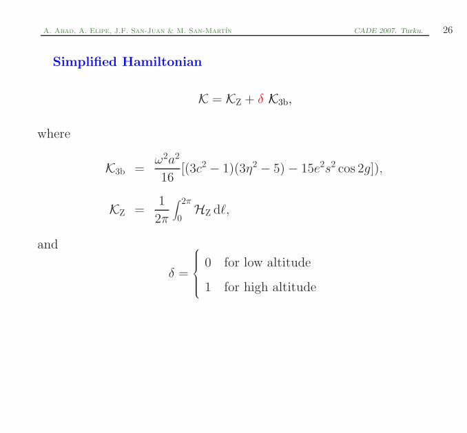
Simplified Hamiltonian
K = KZ + δ K3b,
where
K3b =ω2a2
16[(3c2 − 1)(3η2 − 5) − 15e2s2 cos 2g]),
KZ =1
2π
∫ 2π
0HZ dℓ,
and
δ =
0 for low altitude
1 for high altitude
A. Abad, A. Elipe, J.F. San-Juan & M. San-Martın CADE 2007. Turku. 27
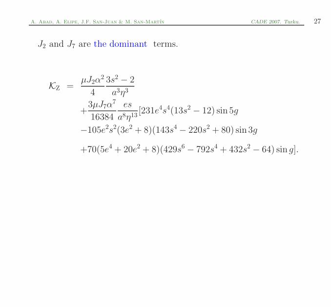
J2 and J7 are the dominant terms.
KZ =µJ2α
2
4
3s2 − 2
a3η3
+3µJ7α
7
16384
es
a8η13[231e4s4(13s2 − 12) sin 5g
−105e2s2(3e2 + 8)(143s4 − 220s2 + 80) sin 3g
+70(5e4 + 20e2 + 8)(429s6 − 792s4 + 432s2 − 64) sin g].
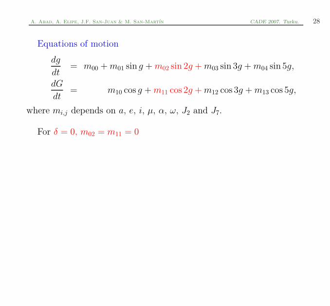
A. Abad, A. Elipe, J.F. San-Juan & M. San-Martın CADE 2007. Turku. 28
Equations of motion
dg
dt= m00 + m01 sin g + m02 sin 2g + m03 sin 3g + m04 sin 5g,
dG
dt= m10 cos g + m11 cos 2g + m12 cos 3g + m13 cos 5g,
where mi,j depends on a, e, i, µ, α, ω, J2 and J7.
For δ = 0, m02 = m11 = 0
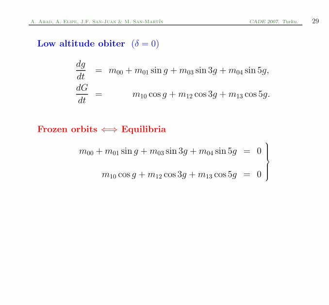
A. Abad, A. Elipe, J.F. San-Juan & M. San-Martın CADE 2007. Turku. 29
Low altitude obiter (δ = 0)
dg
dt= m00 + m01 sin g + m03 sin 3g + m04 sin 5g,
dG
dt= m10 cos g + m12 cos 3g + m13 cos 5g.
Frozen orbits ⇐⇒ Equilibria
m00 + m01 sin g + m03 sin 3g + m04 sin 5g = 0
m10 cos g + m12 cos 3g + m13 cos 5g = 0

A. Abad, A. Elipe, J.F. San-Juan & M. San-Martın CADE 2007. Turku. 30
Low altitude frozen orbits
m00 + m01 sin g + m03 sin 3g + m04 sin 5g = 0,
m10 cos g + m12 cos 3g + m13 cos 5g = 0,
g = π/2, 3π/2
0
0.5
1
1.5
00.050.10.1511.051.11.151.2
11.051.1
a
e
i
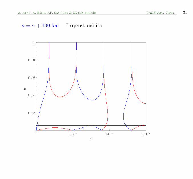
A. Abad, A. Elipe, J.F. San-Juan & M. San-Martın CADE 2007. Turku. 31
a = α + 100 km Impact orbits
0 30 ° 60 ° 90 °i
0.2
0.4
0.6
0.8
1
e
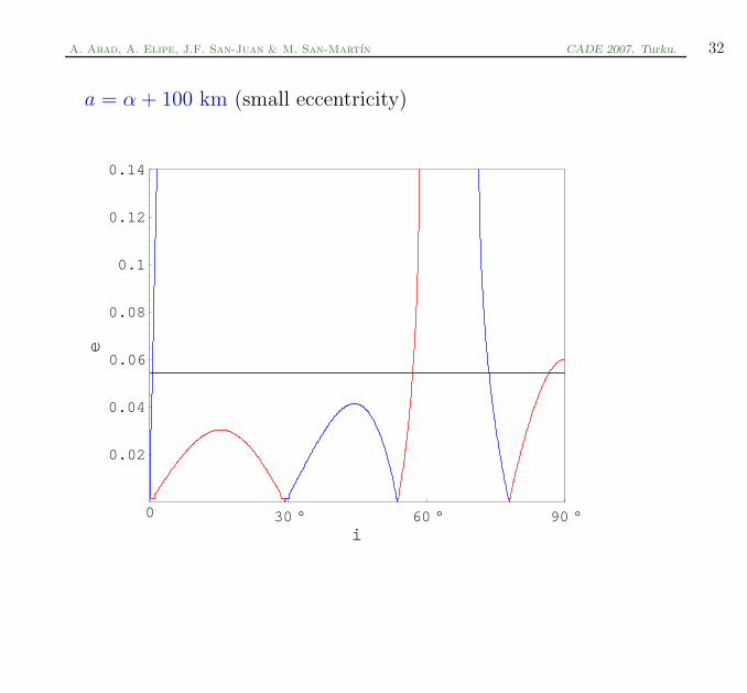
A. Abad, A. Elipe, J.F. San-Juan & M. San-Martın CADE 2007. Turku. 32
a = α + 100 km (small eccentricity)
0 30 ° 60 ° 90 °i
0.02
0.04
0.06
0.08
0.1
0.12
0.14
e
A. Abad, A. Elipe, J.F. San-Juan & M. San-Martın CADE 2007. Turku. 33
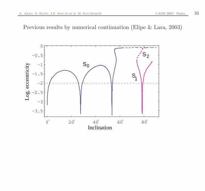
Previous results by numerical continuation (Elipe & Lara, 2003)
0 20 40 60 80
-3.5
-3
-2.5
-2
-1.5
-1
-0.5
0
Log
. ecc
entr
icity
Inclination
o o o o o
S
S
S
0
1
2
A. Abad, A. Elipe, J.F. San-Juan & M. San-Martın CADE 2007. Turku. 34
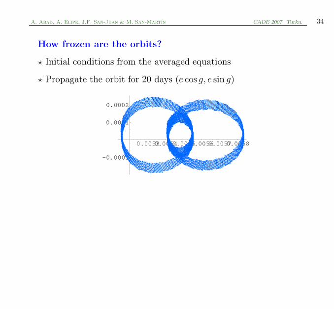
How frozen are the orbits?
⋆ Initial conditions from the averaged equations
⋆ Propagate the orbit for 20 days (e cos g, e sin g)
0.00530.00540.00550.00560.00570.0058
-0.0001
0.0001
0.0002
A. Abad, A. Elipe, J.F. San-Juan & M. San-Martın CADE 2007. Turku. 35
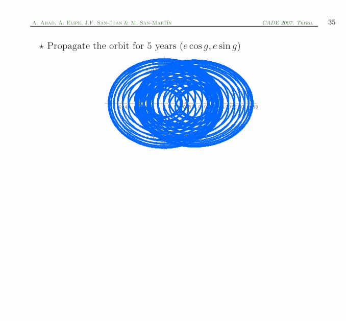
⋆ Propagate the orbit for 5 years (e cos g, e sin g)
0.0046 0.0048 0.0052 0.0054 0.0056 0.0058
-0.0004
-0.0002
0.0002
0.0004
A. Abad, A. Elipe, J.F. San-Juan & M. San-Martın CADE 2007. Turku. 36
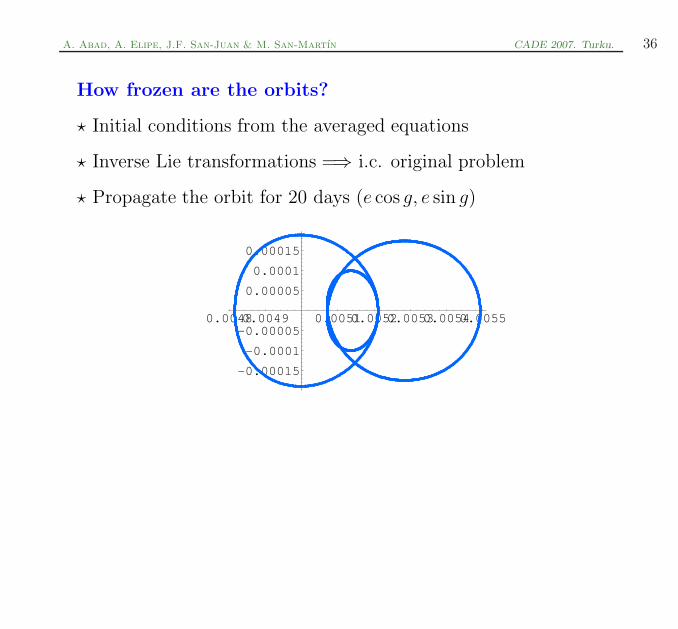
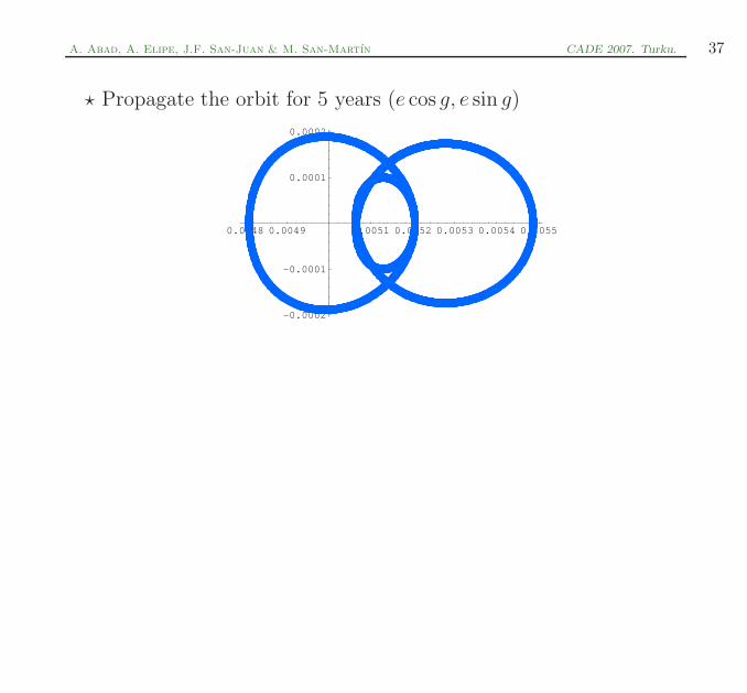
How frozen are the orbits?
⋆ Initial conditions from the averaged equations
⋆ Inverse Lie transformations =⇒ i.c. original problem
⋆ Propagate the orbit for 20 days (e cos g, e sin g)
0.00480.0049 0.00510.00520.00530.00540.0055
-0.00015
-0.0001
-0.00005
0.00005
0.0001
0.00015
A. Abad, A. Elipe, J.F. San-Juan & M. San-Martın CADE 2007. Turku. 37
⋆ Propagate the orbit for 5 years (e cos g, e sin g)
0.0048 0.0049 0.0051 0.0052 0.0053 0.0054 0.0055
-0.0002
-0.0001
0.0001
0.0002
A. Abad, A. Elipe, J.F. San-Juan & M. San-Martın CADE 2007. Turku. 38
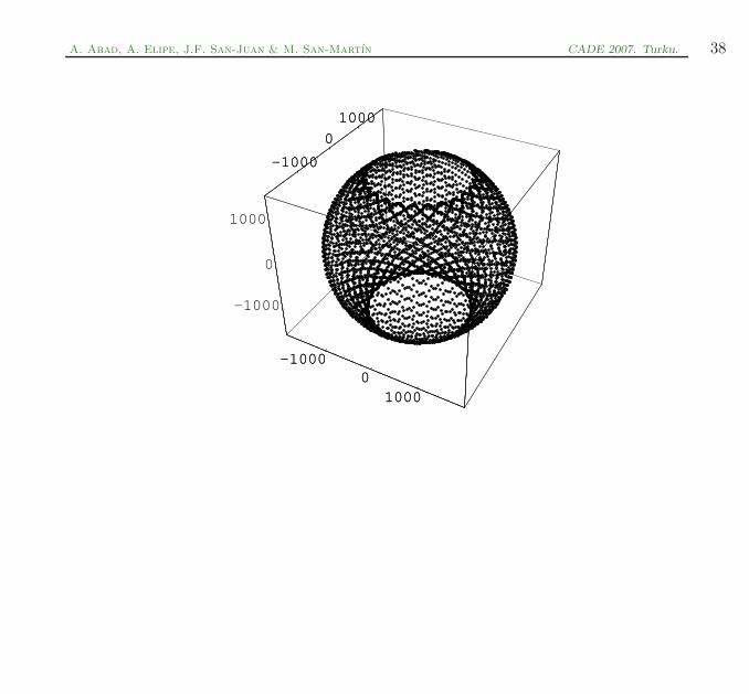
-10000
1000
-1000
0
1000
-1000
0
1000
-10000
1000
-1000
0
1000
A. Abad, A. Elipe, J.F. San-Juan & M. San-Martın CADE 2007. Turku. 39
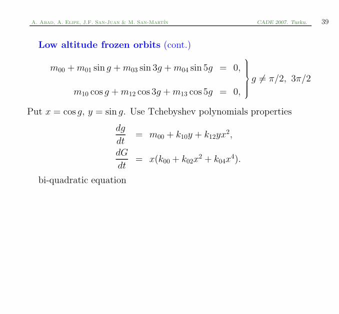
Low altitude frozen orbits (cont.)
m00 + m01 sin g + m03 sin 3g + m04 sin 5g = 0,
m10 cos g + m12 cos 3g + m13 cos 5g = 0,
g 6= π/2, 3π/2
Put x = cos g, y = sin g. Use Tchebyshev polynomials properties
dg
dt= m00 + k10y + k12yx2,
dG
dt= x(k00 + k02x
2 + k04x4).
bi-quadratic equation
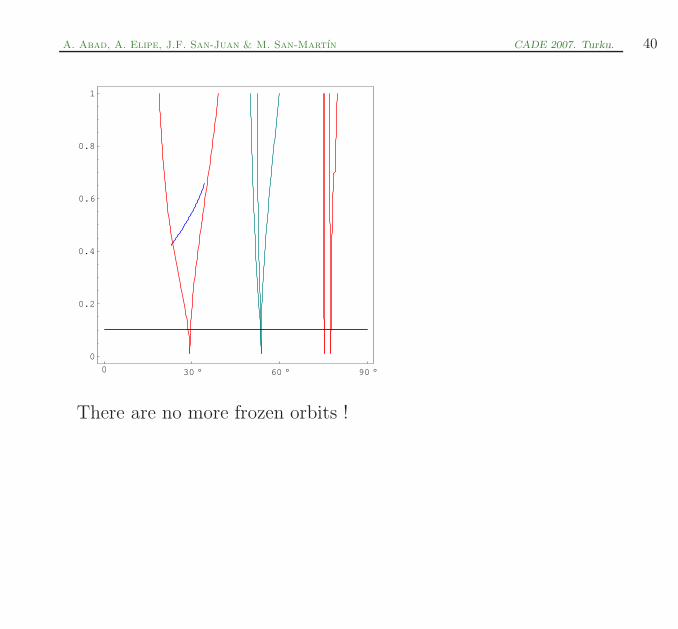
A. Abad, A. Elipe, J.F. San-Juan & M. San-Martın CADE 2007. Turku. 40
0 30 ° 60 ° 90 °
0
0.2
0.4
0.6
0.8
1
There are no more frozen orbits !
A. Abad, A. Elipe, J.F. San-Juan & M. San-Martın CADE 2007. Turku. 41
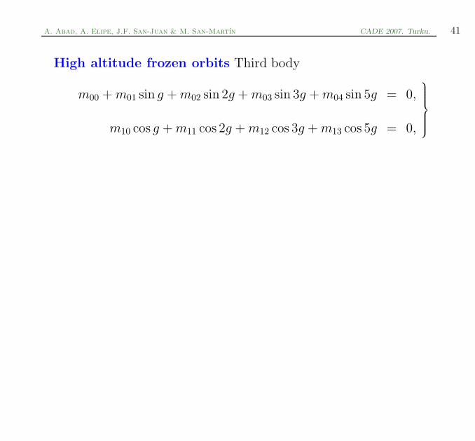
High altitude frozen orbits Third body
m00 + m01 sin g + m02 sin 2g + m03 sin 3g + m04 sin 5g = 0,
m10 cos g + m11 cos 2g + m12 cos 3g + m13 cos 5g = 0,
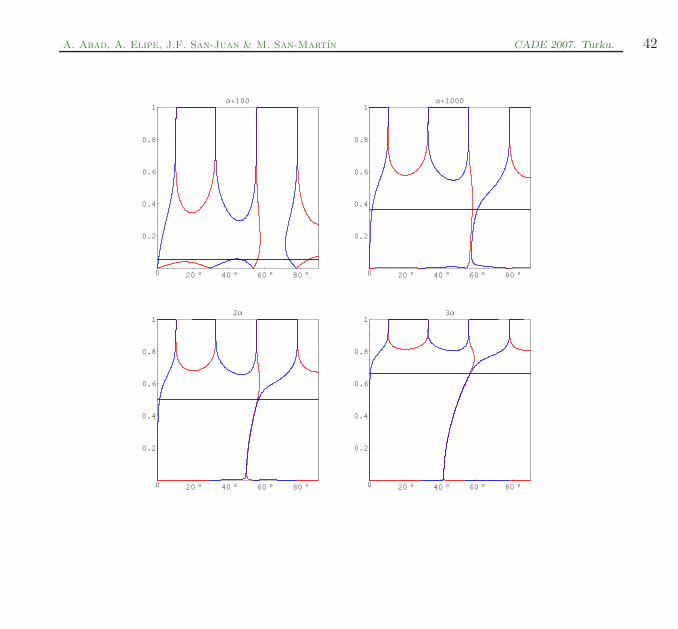
A. Abad, A. Elipe, J.F. San-Juan & M. San-Martın CADE 2007. Turku. 42
0 20 ° 40 ° 60 ° 80 °
0.2
0.4
0.6
0.8
1Α+100
0 20 ° 40 ° 60 ° 80 °
0.2
0.4
0.6
0.8
1Α+1000
0 20 ° 40 ° 60 ° 80 °
0.2
0.4
0.6
0.8
12Α
0 20 ° 40 ° 60 ° 80 °
0.2
0.4
0.6
0.8
13Α