alberto bisin dept. of economics nyu november 9, 2009 notes micro1.pdf · general equilibrium...
TRANSCRIPT

General equilibrium theoryLecture notes
Alberto Bisin
Dept. of Economics
NYU
November 9, 2009

Contents
Preface ix
1 Introduction 1
2 Demand theory: A quick review 3
3 Arrow-Debreu economies 53.1 Competitive equilibrium . . . . . . . . . . . . . . . . . . . . . 53.2 Existence . . . . . . . . . . . . . . . . . . . . . . . . . . . . . 53.3 Welfare . . . . . . . . . . . . . . . . . . . . . . . . . . . . . . 53.4 Di¤erentiable approach: A rough primer . . . . . . . . . . . . 5
3.4.1 Mathematical Appendix . . . . . . . . . . . . . . . . . 83.4.2 References . . . . . . . . . . . . . . . . . . . . . . . . . 8
3.5 Strategic foundations . . . . . . . . . . . . . . . . . . . . . . . 9
4 Two-period economies 114.0.1 Time and state contingent commodities . . . . . . . . . 114.0.2 Financial market economy . . . . . . . . . . . . . . . . 144.0.3 No Arbitrage . . . . . . . . . . . . . . . . . . . . . . . 154.0.4 Equilibrium economies and the stochastic discount factor 184.0.5 Arrow theorem . . . . . . . . . . . . . . . . . . . . . . 20
4.1 Constrained Pareto Optimality . . . . . . . . . . . . . . . . . 224.2 Aggregation . . . . . . . . . . . . . . . . . . . . . . . . . . . . 28
4.2.1 The Representative Agent Theorem . . . . . . . . . . . 324.3 Asset Pricing . . . . . . . . . . . . . . . . . . . . . . . . . . . 37
4.3.1 Some classic representation of asset pricing . . . . . . . 37
v

vi CONTENTS
5 Asymmetric information 435.1 The Economy: Moral Hazard and Adverse Selection . . . . . . 455.2 The Symmetric Information Benchmark . . . . . . . . . . . . 475.3 Incentive Constrained Pareto Optimality . . . . . . . . . . . . 505.4 Walrasian Equilibria: Fully Observable Trades . . . . . . . . . 505.5 Walrasian Equilibria: Non-Observable Trades . . . . . . . . . 505.6 References . . . . . . . . . . . . . . . . . . . . . . . . . . . . . 50
6 In�nite Horizon Economies 536.1 Bubbles . . . . . . . . . . . . . . . . . . . . . . . . . . . . . . 536.2 . . . . . . . . . . . . . . . . . . . . . . . . . . . . . . . . . . 53

Preface
These notes constitute the material for the second half of the Micro I (�rstyear) graduate course at NYU.Other books: Mas Colell, Gale lecture notes.
ix


Chapter 1
Introduction
1


Chapter 2
Demand theory: A quickreview
3


Chapter 3
Arrow-Debreu economies
3.1 Competitive equilibrium
3.2 Existence
3.3 Welfare
3.4 Di¤erentiable approach: A rough primer
Let an economy be parametrized by the endowment vector ! 2 RLI++ keepingpreferences (ui)i2I �xed. Furthermore, normalize pL = 1 and eliminate theL-th component of the excess demand. Then
z : RL�1++ � RLI++ ! RL�1
represents an aggregate excess demand for an exchange economy ! = (!i)i2I 2RLI++. Assume the economy is such that z (p; !) satis�es the following prop-erties:
1. smoothness: z (p; !) is C1;
2. homogeneity of degree 0: z (�p; !) = z (p; !) ;for any � > 0;
3. Walras Law: pz (p; !) = 0; 8p >> 0;
4. Lower boundedness: 9s such that zl (p; !) > �s, 8l 2 L;
5

6 CHAPTER 3 ARROW-DEBREU ECONOMIES
5. Boundary property:
pn ! p 6= 0; with pl = 0 for some l;) max fz1(pn; !); :::; zL(pn; !)g ! 1
De�nition 1 A p 2 RL++ such that z (p; !) = 0 is regular if Dpz (p; !) hasrank L� 1:
De�nition 2 An economy ! 2 RLI++ is regular if Dpz (p; !) has rank L � 1for any p 2 RL�1++ such that z (p; !) = 0.
De�nition 3 An equilibrium price p 2 RL�1++ is locally unique if 9 an openset P such that p 2 P and for any p0 6= p 2 P , z (p0; !) 6= 0:
Proposition 4 A regular equilibrium price p 2 RL�1++ is locally unique. Fur-thermore, the set of equilibrium prices of an economy ! 2 RLI++ is a smoothmanifold (see Math Appendix) of dimension LI:
Proof. Fix an arbitrary ! 2 RLI++: Since Dpz (p; !) has rank L � 1; byregularity of p, the Inverse function theorem - Local (see Math Appendix)applied to the map z : RL�1++ ! RL�1, directly implies local uniqueness of p 2RL�1++ . Since Dpz (p; !) has rank L�1; by regularity of p, the Inverse functiontheorem - Global (see Math Appendix) applied z : RL�1++ � RLI++ ! RL�1;directly implies that the set p 2 z�1(0); as a function of ! 2 RLI++, is asmooth manifold of dimension LI:
Proposition 5 Any economy ! in a full measure Lebesgue subset of RLI++is regular.
Proof. The statement follows by the Transversality theorem (see MathAppendix), if z t 0:We now show that z t 0: Pick an arbitrary agent i 2 I: Itwill be su¢ cient to show that, for any (p; !) 2 RL�1++ �RLI++ such that z(p; !) =0; we can �nd a perturbation d!i 2 RL such that dz = D!iz(p; !)d!
i = �d!i:But any perturbation d!i such that pd!i = 0 leaves each agent i 2 I demandunchanged and hence it implies D!iz(p; !)d!
i = �d!i:
De�nition 6 The index i(p; !) of a price p 2 RL�1++ such that z (p; !) = 0is de�ned as
i(p; !) = (�1)L�1sign jDpz (p; !)j :The index i(!) of an economy (ui; !i)i2I is de�ned as
i(!) =X
p:z(p;!)=0
i(p; !):

3.4 DIFFERENTIABLE APPROACH: A ROUGH PRIMER 7
Theorem 7 For any regular economy ! 2 RLI++, i(!) = 1:
Proof. The theorem is a deep mathematical result whose proof is clearlybeyond the scope of this class. Let it su¢ ce to say that the proof reliescrucially on the boundary property of excess demand. Adventurous readermight want to look at Mas Colell (1985), section 5,6, p. 201-15.
Corollary 8 Any regular economy ! 2 RLI++ has an odd number of equilibria.In particular, any regular economy ! 2 RLI++ has at least one equilibrium.
Proposition 9 Any economy ! 2 RLI++ has at least one equilibrium pricep 2 RL�1++ :
Proof. Sketch. Let ! 2 RLI++ be an arbitrary regular economy. Pick theeconomy !0 2 RLI++ such that there exist a unique price p 2 RL�1++ suchthat z(p) = 0; and Dpz(p) has rank L � 1: One such economy can alwaysbe constructed by choosing !0 2 RLI++ to be a Pareto optimal allocation(show that generic regularity holds in the subset of economies with Paretooptimal endowments). Let t! + (1 � t)!0; for 0 � t � 1; represent a 1-dimensional subset of economies. Let z(p; t) be the map z : RL�1++ � [0; 1]induced by z(p; t) = z(p; t! + (1 � t)!0) for given (!; !0): It follows fromthe Inverse function theorem - Global (see Math Appendix) that the set ofequilibrium prices p 2 z�1(0); as a function of t 2 [0; 1], is a smooth manifoldof dimension 1: Since both ! and !0 2 RLI++ are regular, i(!0) = i(!0) = 1by the Index theorem. By the Classi�cation theorem (see Math Appendix),z�1(0) is homeomorphic to a countable set of lines and circles. Along acomponent of z�1(0) (a line or a circle), a change in index occurs when themanifold folds. Regularity of z�1(0) at the boundary, t = 0 and t = 1implies that at least one component of z�1(0) is di¤eomorphic to a line withboundary at t = 0 and t = 1: It looks confusing, but it�s easier with a �gure.Finally, we need to show that the assumption that ! 2 RLI++ is regular is
without loss of generality. In this respect, suppose ! 2 RLI++ is critical (i.e.,not regular). It is easy to show that the regularity of !0 2 RLI++ implies thatthere exists a regular economy !00 2 RLI++ in an open ball of ! 2 RLI++ suchthat
! = t!0 + (1� t)!00; for 0 < t < 1:But since !0 and !00 2 RLI++ are both regular, any economy ! = t!0+(1�t)!00has at least one equilibrium.

8 CHAPTER 3 ARROW-DEBREU ECONOMIES
3.4.1 Mathematical Appendix
Theorem 10 (Inverse function theorem - Local). Let f : Rn++ ! Rn++ beC1: If Df has rank n; at some x 2 Rn++, there exist an open set V � Rn++and a function f�1 : V ! Rn++ such that f(x) 2 V and f�1(f(z)) = z in aneighborhood of x:
De�nition 11 A subset X � Rm+ is a smooth manifold of dimension n if forany x 2 X there exist a neighborhood U � X and a C1 function f : U !Rn++ such that Df has rank n in the whole domain.
Theorem 12 (Inverse function theorem - Global). Let f : Rm++ ! Rn++;m � n; be C1: Suppose that Dxf has rank n for any x 2 Rm++. Thenf�1(0) =
�x 2 Rm++ jf(x) = 0
is a smooth manifold of dimension m� n:
De�nition 13 Let f : Rm++ ! Rn++; m � n; be C1: f is transversal to 0,denoted f t 0; if Df has rank n for any x 2 Rm++ such that f(x) = 0:
Theorem 14 (Transversality). Let f : Rm++ ! Rn++; m � n; be C1 andtransversal to 0, f t 0: Decompose any vector x 2 Rm++ as x =
�x1x2
�; with
x1 2 Rm�n++ ; x2 2 Rn++: Then Dx2f(x) has rank n for all x in a Lebesguemeasure-1 subset of Rm++:
Theorem 15 (Classi�cation). Every smooth manifold of dimension 1 ishomeomorphic to a disjoint union of countably many copies of R (the realline) and S (the circle).
3.4.2 References
The main reference is:
Andreu Mas Colell, The Theory of General Economic Equilibrium: A Dif-ferentiable Approach, Econometric SocietyMonograph, Cambridge Uni-versity Press, Cambridge, 1985.
But, as Andreu told me once, "I do not hate students so much that Iwould give them this book to read." Similar comments hold, in my opinion,for

3.5 STRATEGIC FOUNDATIONS 9
Yves Balasko, Foundations of the Theory of General Equilibrium, AcademicPress, New York, 1988.
You are then left with:
Andreu Mas Colell, Michael D. Whinston, and Jerry R. Green, Microeco-nomic Theory, Oxford University Press, New York, 1995; ch. 17.D.
Andreu Mas Colell, Four Lectures on the Di¤erentiable Approach to GeneralEquilibrium Theory, inMathematical Economics (Montecatini Terme),A. Ambrosetti, F. Gori, and R. Lucchetti (eds), Lecture Notes in Math-ematics, No. 1330, Springer-Verlag, Berlin, 1986.
� � � � � � � � � � � � � � -Production
3.5 Strategic foundations


Chapter 4
Two-period economies
In a two-period pure exchange economy we study �nancial market equilib-ria. In particular, we study the welfare properties of equilibria and theirimplications in terms of asset pricing.In this context, as a foundation for macroeconomics and �nancial eco-
nomics, we study su¢ cient conditions for aggregation, so that the standardanalysis of one-good economies is without loss of generality, su¢ cient condi-tions for the representative agent theorem, so that the standard analysis ofsingle agent economies is without loss of generality.The No-arbitrage theorem and the Arrow theorem on the decentraliza-
tion of equilibria of state and time contingent good economies via �nancialmarkets are introduced as useful means to characterize �nancial market equi-libria.
4.0.1 Time and state contingent commodities
Consider an economy extending for 2 periods, t = 0; 1. Let i 2 f1; :::; Igdenote agents and l 2 f1; :::; Lg physical goods of the economy. In addition,the state of the world at time t = 1 is uncertain. Let f1; :::; Sg denote thestate space of the economy at t = 1. For notational convenience we typicallyidentify t = 0 with s = 0, so that the index s runs from 0 to S:De�ne n = L(S+1): The consumption space is denoted then by X � Rn+.
Each agent is endowed with a vector !i = (!i0; !i1; :::; !
iS), where !
is 2 RL+;
for any s = 0; :::S. Let ui : X �! R denote agent i�s utility function. Wewill assume:
Assumption 1 !i 2 Rn++ for all i
11

12 CHAPTER 4 TWO-PERIOD ECONOMIES
Assumption 2 ui is continuous, strongly monotonic, strictly quasiconcaveand smooth, for all i (see Magill-Quinzii, p.50 for de�nitions and details).Furthermore, ui has a Von Neumann-Morgernstern representation:
ui(xi) = ui(xi0) +
SXs=1
probsui(xis)
Suppose now that at time 0, agents can buy contingent commodities.That is, contracts for the delivery of goods at time 1 contingently to therealization of uncertainty. Denote by xi = (xi0; x
i1; :::; x
iS) the vector of all
such contingent commodities purchased by agent i at time 0, where xis 2 RL+;for any s = 0; :::; S: Also, let x = (x1; :::; xI):Let � = (�0; �1; :::; �S); where �s 2 RL+ for each s; denote the price of
state contingent commodities; that is, for a price �ls agents trade at time 0the delivery in state s of one unit of good l:Under the assumption that the markets for all contingent commodities
are open at time 0, agent i�s budget constraint can be written as1
�0(xi0 � !i0) +
SXs=0
�s(xis � !is) = 0 (4.1)
De�nition 16 An Arrow-Debreu equilibrium is a (x�; ��) such that
1: x�i 2 argmaxui(xi) s.t. �0(xi0 � !i0) +
SXs=0
�s(xis � !is) = 0; and
2:IXi=1
x�i � !is = 0, for any s = 0; 1; :::; S
Observe that the dynamic and uncertain nature of the economy (con-sumption occurs at di¤erent times t = 0; 1 and states s 2 S) does notmanifests itself in the analysis: a consumption good l at a time t and state sis treated simply as a di¤erent commodity than the same consumption goodl at a di¤erent time t0 or at the same time t but di¤erent state s0. This isthe simple trick introduced in Debreu�s last chapter of the Theory of Value.
1We write the budget constraint with equality. This is without loss of generality undermonotonicity of preferences, an assumption we shall maintain.

13
It has the fundamental implication that the standard theory and results ofstatic equilibrium economies can be applied without change to our dynamic)environment. In particular, then, under the standard set of assumptions onpreferences and endowments, an equilibrium exists and the First and SecondWelfare Theorems hold.2
De�nition 17 Let (x�; ��) be an Arrow-Debreu equilibrium. We say that x�
is a Pareto optimal allocation if there does not exist an allocation y 2 XI
such that
1: u(yi) � u(x�i) for any i = 1; :::; I (strictly for at least one i), and
2:IXi=1
yi � !is = 0, for any s = 0; 1; :::; S
Theorem 18 Any Arrow-Debreu equilibrium allocation x� is Pareto Opti-mal.
Proof. By contradiction. Suppose there exist a y 2 X such that 1) and 2)in the de�nition of Pareto optimal allocation are satis�ed. Then, by 1) inthe de�nition of Arrow-Debreu equilibrium, it must be that
��0(yi0 � !i0) +
SXs=0
��s(yis � !is) � 0;
for all i; and
��0(yi0 � !i0) +
SXs=0
��s(yis � !is) > 0;
for at least one i.Summing over i, then
��0
IXi=1
(yi0 � !i0) +SXs=0
��s
IXi=1
(yis � !is) > 0
which contradicts requirement 2) in the de�nition of Pareto optimal alloca-tion.The proof exploits strict monotonicity of preferences. Where?2Having set de�nitions for 2-periods Arrow-Debreu economies, it should be apparent
how a generalization to any �nite T -periods economies is in fact e¤ectively straightforward.In�nite horizon will be dealt with in successive notes.

14 CHAPTER 4 TWO-PERIOD ECONOMIES
4.0.2 Financial market economy
Consider the 2-period economy just introduced. Suppose now contingentcommodities are not traded. Instead, agents can trade in spot markets andin j 2 f1; :::; Jg assets. An asset j is a promise to pay ajs � 0 units of goodl = 1 in state s = 1; :::; S.3 Let aj = (a
j1; :::; a
jS): To summarize the payo¤s
of all the available assets, de�ne the S � J asset payo¤ matrix
A =
0BBB@a11 ::: a
J1
::: :::
a1S ::: aJS
1CCCA :It will be convenient to de�ne as to be the s-th row of the matrix. Note thatit contains the payo¤ of each of the assets in state s.Let p = (p0; p1; :::; pS), where ps 2 RL+ for each s, denote the spot price
vector for goods. That is, for a price pls agents trade one unit of good lin state s: Recall the de�nition of prices for state contingent commodities inArrow-Debreu economies, denoted �: Note the di¤erence. Let good l = 1at each date and state represent the numeraire; that is, p1s = 1, for alls = 0; :::; S.Let xisl denote the amount of good l that agent i consumes in good s. Let
q = (q1; :::; qJ) 2 RJ+, denote the prices for the assets.4 Note that the pricesof assets are non-negative, as we normalized asset payo¤ to be non-negative.Given prices (p; q) and the asset structure A, any agent i picks a con-
sumption vector xi 2 X and a portfolio zi 2 RJ to
maxui(xi)
s.t.
p0(xi0 � !i0) = �qzi
ps(xis � !is) = Asz
i; for s = 1; :::S:
3The non-negativity restriction on asset payo¤s is just for notational simplicity.4Quantities will be row vectors and prices will be column vectors, to avoid the annoying
use of transposes.

15
De�nition 19 A Financial markets equilibrium is a (x�; z�; p�; q�) such that
1: x�i 2 argmaxui(xi) s.t.
p0(xi0 � !i0) = �qzi; and
ps(xis � !is) = asz
i; for s = 1; :::S; and furthermore
2:IXi=1
x�i � !is = 0, for any s = 0; 1; :::; S; andIXi=1
z�i
Financial markets equilibrium is the equilibrium concept we shall careabout. This is because i) Arrow-Debreu markets are perhaps too demanding arequirement, and especially because ii) we are interested in �nancial marketsand asset prices q in particular. Arrow-Debreu equilibrium will be a usefulconcept insofar as it represents a benchmark (about which we have a wealthof available results) against which to measure Financial markets equilibrium.
De�nition 20 Remark 21 The economy just introduced is characterizedby asset markets in zero net supply, that is, no endowments of assets areallowed for. It is straightforward to extend the analysis to assets in positivenet supply, e.g., stocks. In fact, part of each agent i�s endowment (to bespeci�c: the projection of his/her endowment on the asset span, < A >=f� 2 RS : � = Az; z 2 RJg) can be represented as the outcome of an assetendowment, ziw; that is, letting !
i1 = (!
i11; :::; !
i1S), we can write
!i1 = wi1 + Az
iw
and proceed straightforwardly by constructing the budget constraints and theequilibrium notion.
4.0.3 No Arbitrage
Before deriving the properties of asset prices in equilibrium, we shall investsome time in understanding the implications that can be derived from themilder condition of no-arbitrage. This is because the characterization of no-arbitrage prices will also be useful to characterize �nancial markets equilbria.For notational convenience, de�ne the (S + 1)� J matrix
W =
24 �qA
35 :

16 CHAPTER 4 TWO-PERIOD ECONOMIES
De�nition 22 W satis�es the No-arbitrage condition if there does not exista
there does not exist a z 2 RJ such that Wz > 0:5
The No-Arbitrage condition can be equivalently formulated in the follow-ing way. De�ne the span of W to be
< W >= f� 2 RS+1 : � = Wz; z 2 RJg:
This set contains all the feasible wealth transfers, given asset structure A.Now, we can say that W satis�es the No-arbitrage condition if
< W >\RS+1+ = f0g:
Clearly, requiring that W = (�q; A) satis�es the No-arbitrage condition isweaker than requiring that q is an equilibrium price of the economy (withasset structure A). By strong monotonicity of preferences, No-arbitrage isequivalent to requiring the agent�s problem to be well de�ned. The nextresult is remarkable since it provides a foundation for asset pricing basedonly on No-arbitrage.
Theorem 23 (No-Arbitrage theorem)
< W >\RS+1+ = f0g () 9�̂ 2 RS+1++ such that �̂W = 0:
First, observe that there is no uniqueness claim on the �̂, just existence.Next, notice how �̂W = 0 implies �̂� = 0 for all � 2< W > : It then providesa pricing formula for assets:
�̂W =
0BBB@:::
��̂0qj + �̂1aj1 + :::+ �̂SajS
:::
1CCCA =
0BBB@:::
0
:::
1CCCAJx1
and, rearranging, we obtain for each asset j,
qj = �1aj1 + :::+ �Sa
jS; for �s =
�̂s�̂0
(4.2)
5Wz > 0 requires that all components of Wz are � 0 and at least one of them > 0:

17
Note how the positivity of all components of �̂ was necessary to obtain(4.2).Proof. =) De�ne the simplex in RS+1+ as � = f� 2 RS+1+ :
PSs=0 � s = 1g.
Note that by the No-arbitrage condition, < W >T� is empty. The proof
hinges crucially on the following separating result, a version of Farkas Lemma,which we shall take without proof.
Lemma 24 Let X be a �nite dimensional vector space. Let K be a non-empty, compact and convex subset of X. Let M be a non-empty, closed andconvex subset of X. Furthermore, let K and M be disjoint. Then, thereexists �̂ 2 Xnf0g such that
sup�2M
�̂� < inf�2K
�̂� :
Let X = RS+1+ , K = � and M =< W >. Observe that all the requiredproperties hold and so the Lemma applies. As a result, there exists �̂ 2Xnf0g such that
sup�2<W>
�̂� < inf�2�
�̂� : (4.3)
It remains to show that �̂ 2 RS+1++ : Suppose, on the contrary, that thereis some s for which �̂s � 0. Then note that in (4.3 ), the RHS� 0: By (4.3),then, LHS < 0: But this contradicts the fact that 0 2< W > .We still have to show that �̂W = 0, or in other words, that �̂� = 0 for
all � 2< W >. Suppose, on the contrary that there exists � 2< W > suchthat �̂� 6= 0: Since < W > is a subspace, there exists � 2 R such that�� 2< W > and �̂�� is as large as we want. However, RHS is boundedabove, which implies a contradiction.(= The existence of �̂ 2 RS+1++ such that �̂W = 0 implies that �̂� = 0
for all � 2< W > : By contradiction, suppose 9� � 2< W > and such that� � 2 RS+1+ nf0g: Since �̂ is strictly positive, �̂� � > 0; the desired contradiction.
A few �nal remarks to this section.
Remark 25 An asset which pays one unit of numeraire in state s and noth-ing in all other states (Arrow security), has price �s according to (4.2). Suchasset is called Arrow security.

18 CHAPTER 4 TWO-PERIOD ECONOMIES
Remark 26 Is the vector �̂ obtained by the No-arbitrage theorem unique?Notice how (??) de�nes a system of J equations and S unknowns, representedby �. De�ne the set of solutions to that system as
R(q) = f� 2 RS++ : q = �Ag:
Suppose, the matrix A has rank J 0 � J (that it, A has J 0 linearly independentcolumn vectors and J 0 is the e¤ective dimension of the asset space). Ingeneral, then R(q) will have dimension S � J 0. It follows then that, in thiscase, the No-arbitrage theorem restricts �̂ to lie in a S � J 0 + 1 dimensionalset. If we had S linearly independent assets, the solution set has dimensionzero, and there is a unique � vector that solves (??). The case of S linearlyindependent assets is referred to as Complete markets.
Remark 27 Let preferences be Von Neumann-Morgernstern:
ui(xi) = ui(xi0) +X
s=1;:::;S
probsui(xis)
whereX
s=1;:::;S
probs = 1: Let then ms =�sprobs
. Then
qj = E (maj)
In this representation of asset prices the vector m 2 RS++ is called Stochasticdiscount factor.
4.0.4 Equilibrium economies and the stochastic dis-count factor
In the previous section we showed the existence of a vector that provides thebasis for pricing assets in a way that is compatible with equilibrium, albeitmilder than that. In this section, we will strengthen our assumptions andstudy asset prices in a full-�edged economy. Among other things, this willallow us to provide some economic content to the vector �Recall the de�nition of Financial market equilibrium. Let MRSis(x
i)denote agent i�s marginal rate of substitution between consumption of thenumeraire good 1 in state s and consumption of the numeraire good 1 atdate 0:
19
MRSis(xi) =
@ui(xis)
@xi1s
@ui(xi0)
@xi10
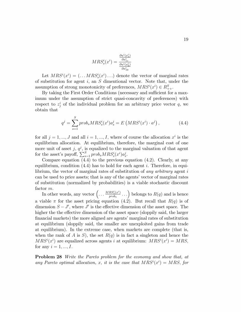
Let MRSi(xi) = (: : :MRSis(xi) : : :) denote the vector of marginal rates
of substitution for agent i, an S dimentional vector. Note that, under theassumption of strong monotonicity of preferences, MRSi(xi) 2 RS++:By taking the First Order Conditions (necessary and su¢ cient for a max-
imum under the assumption of strict quasi-concavity of preferences) withrespect to zij of the individual problem for an arbitrary price vector q, weobtain that
qj =
SXs=1
probsMRSis(x
i)ajs = E�MRSi(xi) � aj
�; (4.4)
for all j = 1; :::; J and all i = 1; :::; I; where of course the allocation xi is theequilibrium allocation. At equilibrium, therefore, the marginal cost of onemore unit of asset j, qj, is equalized to the marginal valuation of that agentfor the asset�s payo¤,
PSs=1 probsMRS
is(x
i)ajs.Compare equation (4.4) to the previous equation (4.2). Clearly, at any
equilibrium, condition (4.4) has to hold for each agent i. Therefore, in equi-librium, the vector of marginal rates of substitution of any arbitrary agent ican be used to price assets; that is any of the agents�vector of marginal ratesof substitution (normalized by probabilities) is a viable stochastic discountfactor m:In other words, any vector
�: : : MRSis(x
i)probs
: : :�belongs to R(q) and is hence
a viable � for the asset pricing equation (4.2). But recall that R(q) is ofdimension S�J 0; where J 0 is the e¤ective dimension of the asset space. Thehigher the the e¤ective dimension of the asset space (sloppily said, the larger�nancial markets) the more aligned are agents�marginal rates of substitutionat equilibrium (sloppily said, the smaller are unexploited gains from tradeat equilibrium). In the extreme case, when markets are complete (that is,when the rank of A is S), the set R(q) is in fact a singleton and hence theMRSi(xi) are equalized across agents i at equilibrium: MRSi(xi) = MRS;for any i = 1; :::; I:
Problem 28 Write the Pareto problem for the economy and show that, atany Pareto optimal allocation, x; it is the case that MRSi(xi) = MRS; for

20 CHAPTER 4 TWO-PERIOD ECONOMIES
any i = 1; :::; I: Furthermore, show that an allocation x which satis�es thefeasibility conditions (market clearing) for goods and is such thatMRSi(xi) =MRS; for any i = 1; :::; I: is Pareto optimal.
We conclude that, when markets are Complete, equilibrium allocationsare Pareto optimal. That is, the First Welfare theorem holds for Financialmarket equilibria when markets are Complete.
Problem 29 (Economies with bid-ask spreads) Extend our economy by as-suming that, given an exogenous vector 2 RJ++:
the buying price of asset j is qj + j
whilethe selling price of asset j is qj
for any j = 1; :::; J:and exogenous. Write the budget constraint and the FirstOrder Conditions for an agent i�s problem. Derive a generalized asset pricingrelation (not an equation, is it?) that relates MRSi(xi) to asset prices.
4.0.5 Arrow theorem
The Arrow theorem is the fondamental decentralization result in �nancialeconomics. It states su¢ cient conditions for a form of equivalence betweenthe Arrow-Debreu and the Financial market equilibrium concepts. It wasessentially introduced by Arrow (1952). The proof of the theorem introducesa reformulation of the budget constraints of the Financial market economywhich focuses on feasible wealth transfers across states directly, on the spanof A,
< A >=�� 2 RS : � = Az; z 2 RJ
in particular. Such a reformulation is important not only in itself but as alemma for welfare analysis in Financial market economies.
Proposition 30 Let (x�; ��) represent an Arrow-Debreu equilibrium. Sup-pose rank(A) = S (�nancial markets are Complete). Then (x�; z�; p�; q�) isa Financial market equilibrium, where
�� = p��: : :MRSis(x
i�)
probs: : :
�and
q� =
SXs=1
probsMRSis(x
i�)as

21
Proof. Financial market equilibrium prices of assets q� satisfy No-arbitrage.There exists then a vector �̂ 2 RS+1++ such that �̂W = 0; or q� = �A. Thebudget constraints in the �nancial market economy are
p�0�xi�0 � !i0
�+ q�zi� = 0
p�s�xi�s � !is
�= asz
i�; for s = 1; :::S:
Substituting q = �A; expanding the �rst equation, and writing the con-straints at time 1 in vector form, we obtain:
p�0�xi�0 � !i0
�+
SXs=1
�sp�s
�xi�s � !is
�= 0 (4.5)26666666664
:
:
p�s (xi�s � !is)
:
:
377777777752 < A > (4.6)
But if rank(A) = S; it follows that< A >= RS; and the constraint
26666666664
:
:
p�s (xi�s � !is)
:
:
377777777752<
A > is never binding. Each agent i�s problem is then subject only to
p�0�xi�0 � !i0
�+
SXs=1
�sp�s
�xi�s � !is
�= 0;
the budget constraint in the Arrow-Debreu economy with
��s = �sp�s; for any s = 1; :::; S:
Furthermore, by No-arbitrage
q� =
SXs=1
probsMRSis(x
i�)as:
22 CHAPTER 4 TWO-PERIOD ECONOMIES
Finally, using �s =MRSis(x
i�)probs
, for any s = 1; :::; S; proves the result. (Recallthat, with Complete markets MRSi(xi�) =MRS; for any i = 1; :::; I.)
4.1 Constrained Pareto Optimality
Under Complete markets, the First Welfare Theorem holds for Financialmarket equilibrium. This is a direct implication of Arrow theorem.
Proposition 31 Let (x�; z�; p�; q�) be a Financial market equilibrium of aneconomy with Complete markets (with rank(A) = S): Then x� is a Paretooptimal allocation.
However, under Incomplete markets Financial market equilibria are gener-ically ine¢ cient in a Pareto sense. That is, a planner could �nd an allocationthat improves some agents without making any other agent worse o¤.
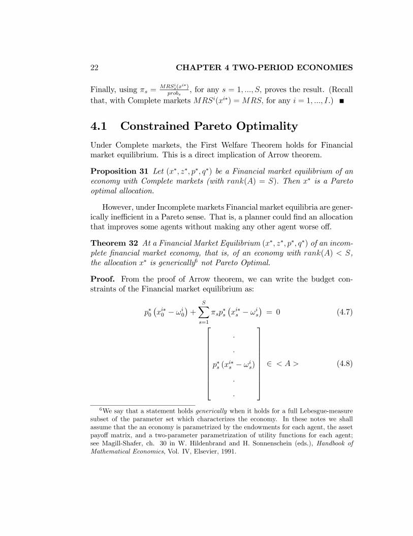
Theorem 32 At a Financial Market Equilibrium (x�; z�; p�; q�) of an incom-plete �nancial market economy, that is, of an economy with rank(A) < S,the allocation x� is generically6 not Pareto Optimal.
Proof. From the proof of Arrow theorem, we can write the budget con-straints of the Financial market equilibrium as:
p�0�xi�0 � !i0
�+
SXs=1
�sp�s
�xi�s � !is
�= 0 (4.7)26666666664
:
:
p�s (xi�s � !is)
:
:
377777777752 < A > (4.8)
6We say that a statement holds generically when it holds for a full Lebesgue-measuresubset of the parameter set which characterizes the economy. In these notes we shallassume that the an economy is parametrized by the endowments for each agent, the assetpayo¤ matrix, and a two-parameter parametrization of utility functions for each agent;see Magill-Shafer, ch. 30 in W. Hildenbrand and H. Sonnenschein (eds.), Handbook ofMathematical Economics, Vol. IV, Elsevier, 1991.

4.1 CONSTRAINED PARETO OPTIMALITY 23
for some � 2 RS++: Pareto optimality of x�requires that there does not existan allocation y such that
1: u(yi) � u(x�i) for any i = 1; :::; I (strictly for at least one i), and
2:
IXi=1
yi � !is = 0, for any s = 0; 1; :::; S
Reproducing the proof of the First Welfare theorem, it is clear that, if such
a y exists, it must be that
26666666664
:
:
p�s (yi�s � !is)
:
:
37777777775=2< A >; for some i = 1; :::; I;
otherwise the allocation y would be budget feasible for all agent i at theequilibrium prices. Generic Pareto sub-optimality of x� follows then directlyfrom the following Lemma, which we leave without proof.7
Lemma 33 Let (x�; z�; p�; q�) represent a Financial Market Equilibrium ofan economy with rank(A) < S: For a generic set of economies, the con-
straints
26666666664
:
:
p�s (xi�s � !is)
:
:
377777777752< A > are binding for some i = 1; :::; I.
Remark 34 The Lemma implies a slightly stronger result than generic Paretosub-optimality of Financial market equilibrium for economies with incompletemarkets. It implies in fact that a Pareto improving allocation can be foundlocally around the equilibrium, as a perturbation of the equilibrium.
7The proof can be found in Magill-Shafer, ch. 30 in W. Hildenbrand and H. Sonnen-schein (eds.), Handbook of Mathematical Economics, Vol. IV, Elsevier, 1991. It requiresmathematical tecniques from di¤erential topology which are not appropriate to be intro-duced in this course.

24 CHAPTER 4 TWO-PERIOD ECONOMIES
Pareto optimality might however represent too strict a de�nition of socialwelfare of an economy with frictions which restrict the consumption set, as inthe case of incomplete markets. In this case, markets are assumed incompleteexogenously. There is no reason in the fundamentals of the model why theyshould be, but they are. Under Pareto optimality, however, the social welfarenotion does not face the same contraints. For this reason, we typically de�ne aweaker notion of social welfare, Constrained Pareto optimality, by restrictingthe set of feasible allocations to satisfy the same set of constraints on theconsumption set imposed on agents at equilibrium. In the case of incompletemarkets, for instance, the feasible wealth vectors across states are restrictedto lie in the span of the payo¤ matrix. That can be interpreted as theeconomy�s ��nancial technology�and it seems reasonable to impose the sametechnological restrictions on the planner�s reallocations. The formalizationof an e¢ ciency notion capturing this idea follows. Let xit=1 = (x
is)Ss=1 2 RSL+ ;
and similarly pt=1 = (ps)Ss=1 2 RSL+
De�nition 35 (Diamond, 1968; Geanakoplos-Polemarchakis, 1986) Let (x�; z�; p�; q�)represent a Financial market equilibrium of an economy whose consumptionset at time t = 1 is restricted by
xit=1;2 B(pt=1); for any i = 1; :::; I
In this economy, the allocation x� is Constrained Pareto optimal if there doesnot exist a (y; �) such that
1: u(yi) � u(x�i) for any i = 1; :::; I, strictly for at least one i
2:IXi=1
yis � !is = 0, for any s = 0; 1; :::; S
and3: yit=1 2 B(g�t=1(!; �)); for any i = 1; :::; I
where g�t=1(!; �) is a vector of equilibrium prices for spot markets at t = 1opened after each agent i = 1; :::; I has received income transfer A�i:
The constraint on the consumption set restricts only time 1 consump-tion allocations. More general constraints are possible but these formulationis consistent with the typical frictions we encounter in economics, e.g., on�nancial markets. It is important that the constraint on the consumption

4.1 CONSTRAINED PARETO OPTIMALITY 25
set depends in general on g�t=1(!; �), that is on equilibrium prices for spotmarkets opened at t = 1 after income transfers to agents. It implicit identi-�es income transfers (besides consumption allocations at time t = 0) as theinstrument available for Constrained Pareto optimality; that is, it implicitlyconstrains the planner implementing Constraint Pareto optimal allocationsto interact with markets, speci�cally to open spot markets after transfers.On the other hand, the planner is able to anticipate the spot price equilib-rium map, g�t=1(!; �); that is, to internalize the e¤ects of di¤erent transferson spot prices at equilibrium.
Proposition 36 Let (x�; z�; p�; q�) represent a Financial market equilibriumof an economy with complete markets (rank(A) = S) and whose consumptionset at time t = 1 is restricted by
xit=1 2 B � RSL+ ; for any i = 1; :::; IIn this economy, the allocation x� is Constrained Pareto optimal.
Crucially, markets are Complete and B is independent of prices. Theproof is then a straightforward extension of the First Welfare theorem com-bined with Arrow theorem. Constraint Pareto optimality of Financial marketequilibrium allocations is guaranteed as long as the constraint set B is ex-ogenous.
Proposition 37 Let (x�; z�; p�; q�) represent a Financial market equilibriumof an economy with Incomplete markets (rank(A) < S). In this economy,the allocation x� is not Constrained Pareto optimal.
Proof. By the decomposition of the budget constraints in the proof of Arrowtheorem, this economy is equivalent to one with Complete markets whoseconsumption set at time t = 1 is restricted by
xit=1 2 B(g�t=1(!; z)); for any i = 1; :::; I; for any i = 1; :::; Iwith the set B(g�t=1(!; z)) de�ned implicitly by26666666664
:
:
g�s(!s; z) (xis � !is)
:
:
377777777752< A >; for any i = 1; :::; I
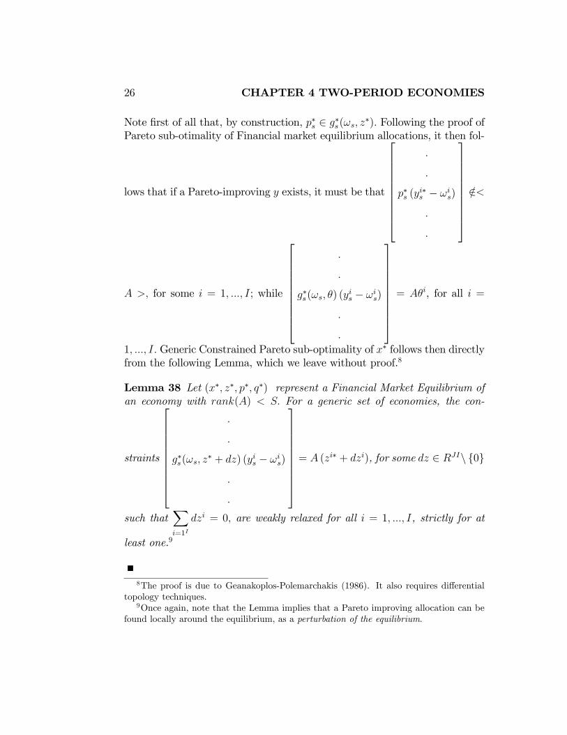
26 CHAPTER 4 TWO-PERIOD ECONOMIES
Note �rst of all that, by construction, p�s 2 g�s(!s; z�): Following the proof ofPareto sub-otimality of Financial market equilibrium allocations, it then fol-
lows that if a Pareto-improving y exists, it must be that
26666666664
:
:
p�s (yi�s � !is)
:
:
37777777775=2<
A >; for some i = 1; :::; I; while
26666666664
:
:
g�s(!s; �) (yis � !is)
:
:
37777777775= A�i, for all i =
1; :::; I: Generic Constrained Pareto sub-optimality of x� follows then directlyfrom the following Lemma, which we leave without proof.8
Lemma 38 Let (x�; z�; p�; q�) represent a Financial Market Equilibrium ofan economy with rank(A) < S: For a generic set of economies, the con-
straints
26666666664
:
:
g�s(!s; z� + dz) (yis � !is)
:
:
37777777775= A (zi� + dzi), for some dz 2 RJIn f0g
such thatXi=1I
dzi = 0; are weakly relaxed for all i = 1; :::; I, strictly for at
least one.9
8The proof is due to Geanakoplos-Polemarchakis (1986). It also requires di¤erentialtopology techniques.
9Once again, note that the Lemma implies that a Pareto improving allocation can befound locally around the equilibrium, as a perturbation of the equilibrium.
4.1 CONSTRAINED PARETO OPTIMALITY 27
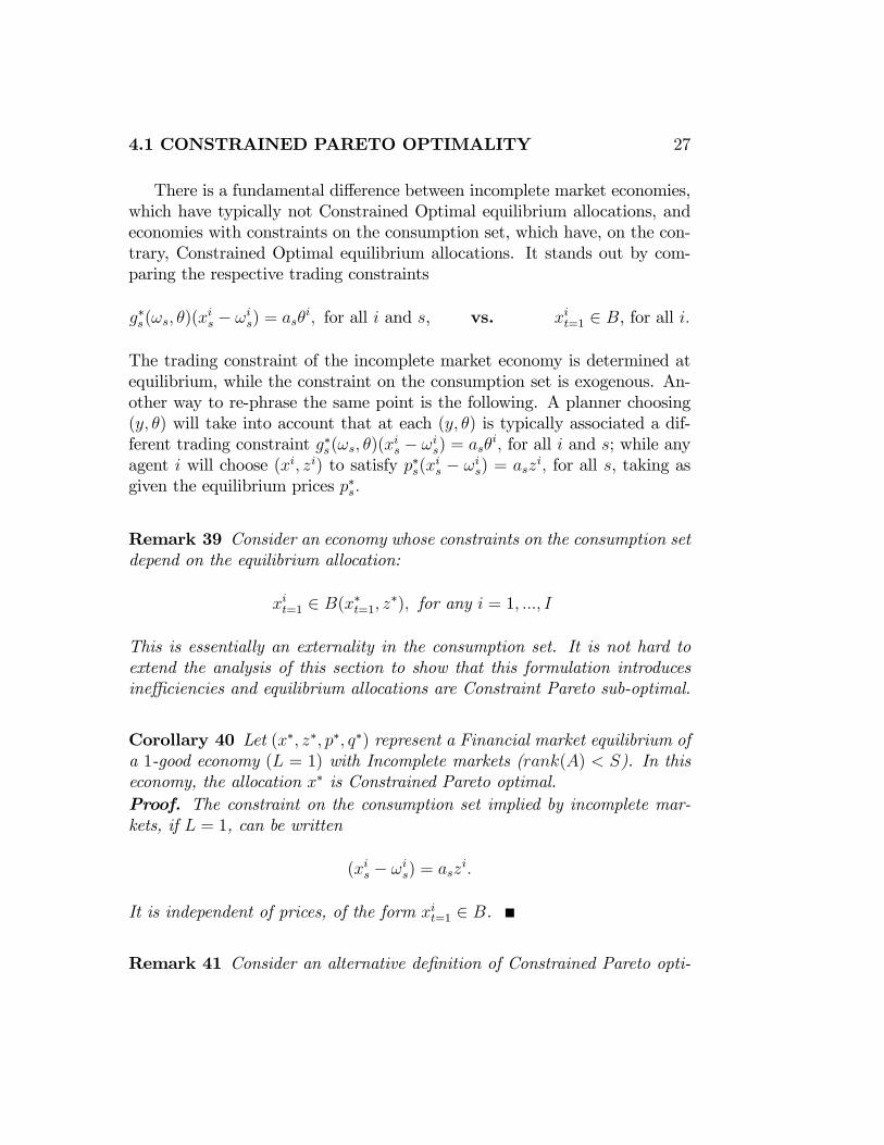
There is a fundamental di¤erence between incomplete market economies,which have typically not Constrained Optimal equilibrium allocations, andeconomies with constraints on the consumption set, which have, on the con-trary, Constrained Optimal equilibrium allocations. It stands out by com-paring the respective trading constraints
g�s(!s; �)(xis � !is) = as�i; for all i and s, vs. xit=1 2 B, for all i:
The trading constraint of the incomplete market economy is determined atequilibrium, while the constraint on the consumption set is exogenous. An-other way to re-phrase the same point is the following. A planner choosing(y; �) will take into account that at each (y; �) is typically associated a dif-ferent trading constraint g�s(!s; �)(x
is � !is) = as�i; for all i and s; while any
agent i will choose (xi; zi) to satisfy p�s(xis � !is) = aszi; for all s, taking as
given the equilibrium prices p�s:
Remark 39 Consider an economy whose constraints on the consumption setdepend on the equilibrium allocation:
xit=1 2 B(x�t=1; z�); for any i = 1; :::; I
This is essentially an externality in the consumption set. It is not hard toextend the analysis of this section to show that this formulation introducesine¢ ciencies and equilibrium allocations are Constraint Pareto sub-optimal.
Corollary 40 Let (x�; z�; p�; q�) represent a Financial market equilibrium ofa 1-good economy (L = 1) with Incomplete markets (rank(A) < S). In thiseconomy, the allocation x� is Constrained Pareto optimal.Proof. The constraint on the consumption set implied by incomplete mar-kets, if L = 1, can be written
(xis � !is) = aszi:
It is independent of prices, of the form xit=1 2 B.
Remark 41 Consider an alternative de�nition of Constrained Pareto opti-

28 CHAPTER 4 TWO-PERIOD ECONOMIES
mality, due to Grossman (1970), in which constraints 3 are substituted by
30:
26666666664
:
:
p�s (xi�s � !is)
:
:
37777777775= Azi; for any i = 1; :::; I
where p� is the spot market Financial market equilibrium vector of prices.That is, the planner takes the equilibrium prices as given. It is immediate toprove that, with this de�nition of Constrained Pareto optimality, any Finan-cial market equilibrium allocation x�of an economy with Incomplete marketsis in fact Constrained Pareto optimal, independently of the �nancial marketsavailable (rank(A) � S):
Problem 42 Consider a Complete market economy (rank(A) = S) whosefeasible set of asset portfolios is restricted by:
zi 2 Z ( RJ ; for any i = 1; :::; I
A typical example is borrowing limits:
zi � �b; for any i = 1; :::; I
Are equilibrium allocations of such an economy Constrained Pareto optimal(also if L > 1)?
Problem 43 Consider a 1-good (L = 1) Incomplete market economy (rank(A) <S) which lasts 3 periods. De�ne an Financial market equilibrium for thiseconomy as well as Constrained Pareto optimality. Are Financial marketequilibrium allocations of such an economy Constrained Pareto optimal?
4.2 Aggregation
Agent i�s optimization problem in the de�nition of Financial market equi-librium requires two types of simultaneous decisions. On the one hand, the

4.2 AGGREGATION 29
agent has to deal with the usual consumption decisions i.e., she has to decidehow many units of each good to consume in each state. But she also hasto make �nancial decisions aimed at transferring wealth from one state tothe other. In general, both individual decisions are interrelated: the con-sumption and portfolio allocations of all agents i and the equilibrium pricesfor goods and assets are all determined simultaneously from the system ofequations formed by (??) and (??). The �nancial and the real sectors ofthe economy cannot be isolated. Under some special conditions, however,the consumption and portfolio decisions of agents can be separated. Thisis typically very useful when the analysis is centered on �nancial issue. Inorder to concentrate on asset pricing issues, most �nance models deal in factwith 1-good economies, implicitly assuming that the individual �nancial de-cisions and the market clearing conditions in the assets markets determinethe �nancial equilibrium, independently of the individual consumption deci-sions and market clearing in the goods markets; that is independently of thereal equilibrium prices and allocations. In this section we shall identify theconditions under which this can be done without loss of generality. This issometimes called "the problem of aggregation."The idea is the following. If we want equilibrium prices on the spot
markets to be independent of equilibrium on the �nancial markets, thenthe aggregate spot market demand for the L goods in each state s shouldmust depend only on the incomes of the agents in this state (and not inother states) and should be independent of the distribution of income amongagents in this state.
Theorem 44 Budget Separation. Suppose that each agent i�s prefer-ences are separable across states, identical, homothetic within states, andvon Neumann-Morgenstern; i.e. suppose that there exists an homotheticu : RL ! R such that
ui(xi) = u(xi0) +SXs=1
probsu(xis); for all i = 1; ::; I:
Then equilibrium spot prices p� are independent of asset prices q and of theincome distribution; that is, constant in
n!i 2 RL(S+1)++
���PIi=1 !
i giveno:
Proof. The consumer�s maximization problem in the de�nition of Financialmarket equilibrium can be decomposed into a sequence of spot commodity

30 CHAPTER 4 TWO-PERIOD ECONOMIES
allocation problems and an income allocation problem as follows. The spotcommodity allocation problems. Given the current and anticipated spot pricesp = (p0; p1; :::; pS) and an exogenously given stream of �nancial income yi =(yi0; y
i1; :::; y
iS) 2 RS+1++ in units of numeraire, agent i has to pick a consumption
vector xi 2 RL(S+1)+ to
maxui(xi)
s:t:
p0xi0 = y
i0
psxis = y
is; for s = 1; :::S:
Let the L(S + 1) demand functions be given by xils(p; yi), for l = 1; :::; L;
s = 0; 1; :::S. De�ne now the indirect utility function for income by
vi(yi; p) = ui(xi(p; yi)):
The Income allocation problem. Given prices (p; q); endowments !i, and theasset structure A, agent i has to pick a portfolio zi 2 RJ and an incomestream yi 2 RS+1++ to
max vi(yi; p)
s:t:
p0!i0 � qzi = yi0
ps!is + asz
i = yis; for s = 1; :::S:
By additive separability across states of the utility, we can break the con-sumption allocation problem into S+1 �spot market�problems, each of whichyields the demands xis(ps; y
is) for each state. By homotheticity, for each
s = 0; 1; :::S; and by identical preferences across all agents,
xis(ps; yis) = y
isxis(ps; 1);
and since preferences are identical across agents,
yisxis(ps; 1) = y
isxs(ps; 1)

4.2 AGGREGATION 31
Adding over all agents and using the market clearing condition in spot mar-kets s, we obtain, at spot markets equilibrium,
xs(p�s; 1)
IXi=1
yis �IXi=1
!is = 0:
Again by homothetic utility,
xs(p�s;
IXi=1
yis)�IXi=1
!is = 0: (4.9)
Recall from the consumption allocation problem that psxis = yis; for s =0; 1; :::S: By adding over all agents, and using market clearing in the spotmarkets in state s,
IXi=1
yis = p�s
IXi=1
xis; for s = 0; 1; :::S (4.10)
= p�s
IXi=1
!is; for s = 0; 1; :::S:
By combining (4.9) and (4.10), we obtain
xs(p�s; p
�s
IXi=1
!is) =IXi=1
!is: (4.11)
Note how we have passed from the aggregate demand of all agents in theeconomy to the demand of an agent owning the aggregate endowments. Ob-serve also how equation (4.11) is a system of L equations with L unknownsthat determines spot prices p�s for each state s independently of asset pricesq: Note also that equilibrium spot prices p�s de�ned by (4.11) only depend !
i
throughPI
i=1 !is:
Remark 45 The Budget separation theorem can be interpreted as identifyingconditions under which studying a single good economy is without loss ofgenerality. To this end, consider the income allocation problem of agent i,

32 CHAPTER 4 TWO-PERIOD ECONOMIES
given equilibrium spot prices p� :
maxyi2RS+1++
vi(yi; p�)
s:t:
yi0 = p�0!i0 � qzi
yis = p�s!is + asz
i; for s = 1; :::S
If preferences separable across states, identical, homothetic within states, andvon Neumann-Morgenstern, it is straightforward to show that vi(yi; p�) isidentical across agents i and, seen as a function of yi, it satis�es the as-sumptions we have imposed on ui as a function of xi, in Assumption A.2.Let w0 = p�0!
i0; ws = p
�s!
is; for any s = 1; :::; S; and disregard for notational
simplicity the dependence of vi(yi; p�) on p�: The income allocation problembecomes:
maxyi2RS+1++
v(yi)
s:t:
yi0 � w0 = �qzi
yis � ws = aszi; for s = 1; :::S
which is homeomorphic to any agent i�s optimization problem in the de�-nition of Financial market equilibrium with l = 1. Note that yis gains theinterpretation of agent i�s consumption expenditure in state s, while ws isinterpreted as agent i�s income endowment in state s:
4.2.1 The Representative Agent Theorem
A representative agent is the following theoretical construct.
De�nition 46 Consider a Financial market equilibrium (x�; z�; p�; q�) of aneconomy populated by i = 1; :::; I agents with preferences ui : X ! R andendowments !i: A Representative agent for this economy is an agent withpreferences UR : X ! R and endowment !R such that the Financial marketequilibrium of an associated economy with the Representative agent as theonly agent has prices (p�; q�).

4.2 AGGREGATION 33
In this section we shall identify assumptions which guarantee that theRepresentative agent construct can be invoked without loss of generality.This assumptions are behind much of the empirical macro/�nance literature.
Theorem 47 Representative agent. Suppose there exists an homotheticu : RL ! R such that
ui(xi) = u(xi0) +SXs=1
probsu(xis); for all i = 1; ::; I:
Let p� denote equilibrium spot prices. If p�s!is 2< A >; then there exist a
map uR : RS+1 ! R such that:
!R =IXi=1
!is;
UR(x) = uR(y0) +SXs=1
probsuR(ys) where ys = p�
IXi=1
xis; s = 0; 1; :::; S
constitutes a Representative agent.
Since the Representative agent is the only agent in the economy, herconsumption allocation and portfolio at equilibrium,
�x�R; z�R
�; are:
x�R = !R =IXi=1
!i
z�R = 0
If the Representative agent�s preferences can be constructed indepen-dently of the equilibrium of the original economy with I agents, then equilib-rium prices can be read out of the Representative agent�s marginal rates ofsubstitution evaluated at
PIi=1 !
i. SincePI
i=1 !i is exogenously given, equi-
librium prices are obtained without computing the consumption allocationand portfolio for all agents at equilibrium, (x�; z�):Proof. The proof is constructive. Under the assumptions on preferences inthe statement, we need to show that, for all agents i = 1; :::; I, equilibriumasset prices q� are constant in
n!i 2 RL(S+1)++
���PIi=1 !
i giveno.If preferences

34 CHAPTER 4 TWO-PERIOD ECONOMIES
satisfy ui(xi) = u(xi0) +PS
s=1 probsu(xis); for all i = 1; ::; I, with an homo-
thetic u; by the Budget separation theorem, equilibrium spot prices p� areindependent of q� and constant in
n!i 2 RL(S+1)++
���PIi=1 !
i giveno: There-
fore, p�s!is 2< A > is an assumption on fundamentals; in particular on !i:
Furthermore, we can restrict our analysis to the single good economy derivedin the previous remark, whose agent i�s optimization problem is:
maxyi2RS+1++
v(yi)
s:t:
yi0 � w0 = �qzi
yis � ws = aszi; for s = 1; :::S
Write the budget constraints
yi0 � w0 = �qzi
yis � ws = aszi; for s = 1; :::S
as
26666664yi0 � w0:
yis � ws:
37777775 2<��qA
�>. Under the homothetic representation of prefer-
ences ui(xi), we can show that v(yi) is von Neumann-Morgernstern and
v(yi) = uR(yi0) +SXs=1
probsuR(yis)
for some function uR : R ! R: By Arrow theorem�we can write budgetconstraints as
yi0 � wi0 +SXs=1
�s�yis � ws
�= 0�
yis � wis�Ss=1
2 < A >
But, (wis)Ss=1 2< A > implies that there exist a ziw such that (ws)
Ss=1 = Az
iw:
Therefore, (wis)Ss=1 2< A > implies that (yis)
Ss=1 = A (z
i + ziw) :We can then

4.2 AGGREGATION 35
write each agent i�s optimization problem in terms of (yi0 � wi0; zi); and thevalue of agent i0s endowment is wi0+
PSs=1 �sw
is = +
PSs=1 �sasz
iw = w
i0+qz
iw:
By the fact that preferences are identical across agents and by homotheticityof v; then we can write�yi0 (q; w
i0 + qz
iw)� wi0
zi (q; wi0 + qziw)
�=
�y0 (q; w
i0 + qz
iw)� wi0
z (q; wi0 + qziw)
�=�wi0 + qz
iw
� �y0 (q; 1)� wi0z (q; 1)
�At equilibrium then
�y0 (q
�; 1)� wi0z (q�; 1)
� IXi=1
�wi0 + q
�ziw�=
�y0 �q�;PIi=1w
i0 + q
�PIi=1 z
iw
��PI
i=1wi0
z�q�;PI
i=1wi0 + q
�PIi=1 z
iw
� �=
=
�0
0
�:
and prices q� only depend onPI
i=1wi0 and
PIi=1 z
iw: But since (w
is)Ss=1 = Az
iw;PI
i=1 ziw is a linear translation of
PIi=1w
i: Finally, let
UR(x) = v(IXi=1
yi) where yis = p�
IXi=1
xis; s = 0; 1; :::; S
to end the proof.The Representative agent theorem, as noted, allows us to obtain equilib-
rium prices without computing the consumption allocation and portfolio forall agents at equilibrium, (x�; z�):Let w =
PIi=1w
i: Under the assumptionsof the Representative agent theorem,
q =
SXs=1
MRSs(w)as; for MRSs(w) =@uR(ws)@ws
@uR(w0)@w0
That is, asset prices can be computed from agents�preferences uR : R ! Rand from the aggregate endowment w: This is called the Lucas� trick forpricing assets.
Problem 48 Note that, under the Complete markets assumption, the spanrestriction on endowments, p�s!
is 2< A >; is trivially satis�ed. Does the
assumption p�s!is 2< A >; for all agents i imply Pareto optimal allocations
in equilibrium.
36 CHAPTER 4 TWO-PERIOD ECONOMIES
Problem 49 Assume all agents have identical quadratic preferences. Deriveindividual demands for assets (without assuming p�s!
is 2< A >) and show
that the Representative agent theorem is obtained.
Another interesting but misleading result is the "weak" representativeagent theorem, due to Constantinides (1982).
Theorem 50 Suppose markets are complete (rank(A) = S) and preferencesui(xi) are von Neumann-Morgernstern (but not necessarily identical nor ho-mothetic). Let (x�; z�; p�; q�) be a Financial markets equilibrium. Then,
!R =IXi=1
!i;
UR(x) = max(xi)Ii=1
IXi=1
�iui(xi) s.t.IXi=1
xi = x; where �i = (�i)�1 and �i =
@ui(xi�)
@xi�10
constitutes a Representative agent.
Clearly, then,
q� =SXs=1
MRSRs (!Rs )as;
where MRSRs (x) =@UR(x)@xs
@UR(x)@x0
:
Proof. Consider a Financial market equilibrium (x�; z�; p�; q�). By completemarkets, the First welfare theorem holds and x� is a Pareto optimal alloca-tion. Therefore, there exist some weights that make x� the solution to theplanner�s problem. It turns out that the required weights are given by
�i =
�@ui(xi�)
@xi�10
��1:
This is left to the reader to check; it�s part of the celebrated Negishi theorem..
This result is certainly very general, as it does not impose identical ho-mothetic preferences, however, it is not as useful as the �real�Representativeagent theorem to �nd equilibrium asset prices. The reason is that to de�nethe speci�c weights for the planner�s objective function, (�i)Ii=1; we need toknow what the equilibrium allocation, x�; which in turn depends on the wholedistribution of endowments over the agents in the economy.

4.3 ASSET PRICING 37
4.3 Asset Pricing
Relying on the aggregation theorem in the previous section, in this sectionwe will abstract from the consumption allocation problems and concentrateon one-good economies. This allows us to simplify the equilibrium de�nitionas follows.
4.3.1 Some classic representation of asset pricing
Often in �nance, especially in empirical �nance, we study asset pricing rep-resentation which express asset returns in terms of risk factors. Factors areto be interpreted as those component of the risks that agents do require ahigher return to hold.How do we go from our basic asset pricing equation
q = E(mA)
to factors?
Single factor beta representation
Consider the basic asset pricing equation for asset j;
qj = E(maj)
Let the return on asset j, Rj, be de�ned as Rj =Ajqj. Then the asset pricing
equation becomes1 = E(mRj)
This equation applied to the risk free rate, Rf , becomes Rf = 1Em. Using the
fact that for two random variables x and y, E(xy) = ExEy + cov(x; y), wecan rewrite the asset pricing equation as:
ERj =1
Em� cov(m;Rj)
Em= Rf � cov(m;Rj)
Em
or, expressed in terms of excess return:
ERj �Rf = �cov(m;Rj)
Em
38 CHAPTER 4 TWO-PERIOD ECONOMIES
Finally, letting
�j = �cov(m;Rj)
var(m)
and
�� =var(m)
Em
we have the beta representation of asset prices:
ERj = Rf + �j�m (4.12)
We interpret �j as the "quantity" of risk in asset j and �m (which is thesame for all assets j) as the "price" of risk. Then the expected return ofan asset j is equal to the risk free rate plus the correction for risk, �j�m.Furthermore, we can read (4.12) as a single factor representation for assetprices, where the factor is m, that is, if the representative agent theoremholds, her intertemporal marginal rate of substitution.
Multi-factor beta representations
A multi-factor beta representation for asset returns has the following form:
ERj = Rf +FXf=1
�jf�mf(4.13)
where (mf )Ff=1 are orthogonal random variables which take the interpretation
of risk factors and
�jf = �cov(mf ; Rj)
var(mf )
is the beta of factor f , the loading of the return on the factor f .
Proposition 51 A single factor beta representation
ERj = Rf + �j�m
is equivalent to a multi-factor beta representation
ERj = Rf +
FXf=1
�jf�mfwith m =
FXf=1
bfmf

4.3 ASSET PRICING 39
In other words, a multi-factor beta representation for asset returns isconsistent with our basic asset pricing equation when associated to a linearstatistical model for the stochastic discount factor m, in the form of m =PF
f=1 bfmf .
Proof. Write 1 = E(mRj) as Rj = Rf � cov(m;Rj)
Emand then to substitute
m =PF
f=1 bfmf and the de�nitions of �jf , to have
�mf=var(mf )bfEmf
The CAPM
The CAPM is nothing else than a single factor beta representation of thefollowing form:
ERj = Rf + �jf�mf
wheremf = a+ bR
w
the return on the market portfolio, the aggregate portfolio held by the in-vestors in the economy.It can be easily derived from an equilibrium model under special assump-
tions.For example, assume preferences are quadratic:
u(xio; xi1) = �
1
2(xi � x#)2 � 1
2�
SXs=1
probs(xis � x#)2
Moreover, assume agents have no endowments at time t = 1. LetPI
i=1 xis =
xs; s = 0; 1; :::; S; andPI
i=1wi0 = w0. Then budget constraints include
xs = Rws (w0 � x0)
Then,
ms = �xs � x#x0 � x#
=�(w0 � x0)(x0 � x#)
Rws ��x#
x0 � x#
which is the CAPM for a = � �x#
x0�x# and b =�(w0�x0)(x0�x#) :

40 CHAPTER 4 TWO-PERIOD ECONOMIES
Note however that a = �x#
x0�x# and b =�(w0�x0)(x0�x#) are not constant, as they
do depend on equilibrium allocations. This will be important when we studyconditional asset market representations, as it implies that the CAPM isintrinsically a conditional model of asset prices.
Bounds on stochastic discount factors
Write the beta representation of asset returns as:
ERj �Rf = cov(m;Rj)
Em=�(m;Rj)�(m)�(Rj)
Emwhere 0 � �(m;Rj) � 1 denotes the correlation coe¢ cient and �(:), thestandard deviation. Then
j ERj �Rf�(Rj)
j� �(m)
Em
The left-hand-side is the Sharpe-ratio of asset j.The relationship implies a lower bound on the standard deviation of any
stochastic discount factor m which prices asset j. Hansen-Jagannathan areresponsible for having derived bounds like these and shown that, when thestochastic discount factor is assumed to be the intertemporal marginal rateof substitution of the representative agent (with CES preferences), the datadoes not display enough variation in m to satisfy the relationship.
A related bound is derived by noticing that no-arbitrage implies the ex-istence of a unique stochastic discount factor in the space of asset payo¤s,denoted mp, with the property that any other stochastic discount factor msatis�es:
m = mp + �
where � is orthogonal to mp.The following corollary of the No-arbitrage theorem leads us to this result.
Corollary 52 Let (A; q) satisfy No-arbitrage. Then, there exists a unique� � 2< A > such that q = A� �:
Proof. By the No-arbitrage theorem, there exists � 2 RS++ such that q = �A:We need to distinguish notationally a matrix M from its transpose, MT :Wewrite then the asset prices equation as qT = AT�T . Consider �p:
�Tp = A(ATA)�1q:

4.3 ASSET PRICING 41
Clearly, qT = AT�Tp ; that is, �Tp satis�es the asset pricing equation. Further-
more, such �Tp belongs to < A >, since �Tp = Azp for zp = (ATA)�1q: Prove
uniqueness.We can now exploit this uniqueness result to yield a characterization of
the �multiplicity�of stochastic discount factors when markets are incomplete,and consequently a bound on �(m). In particular, we show that, for a given(q; A) pair a vector m is a stochastic discount factor if and only if it canbe decomposed as a projection on < A > and a vector-speci�c componentorthogonal to < A >. Moreover, the previous corollary states that such aprojection is unique.
Let m 2 RS++ be any stochastic discount factor, that is, for any s =1; : : : ; S, ms =
�sprobs
and qj = E(mAj); for j = 1; :::; J: Consider the orthogo-nal projection of m onto < A >, and denote it by mp. We can then write anystochastic discount factors m as m = mp + ", where " is orthogonal to anyvector in < A >; in particular to any Aj. Observe in fact that mp+ " is alsoa stochastic discount factors since qj = E((mp+")aj) = E(mpaj)+E("aj) =E(mpaj), by de�nition of ". Now, observe that qj = E(mpaj) and that wejust proved the uniqueness of the stochastic discount factors lying in < A > :In words, even though there is a multiplicity of stochastic discount factors,they all share the same projection on < A >. Moreover, if we make the eco-nomic interpretation that the components of the stochastic discount factorsvector are marginal rates of substitution of agents in the economy, we caninterpret mp to be the economy�s aggregate risk and each agents " to be theindividual�s unhedgeable risk.It is clear then that
�(m) � �(mp)
the bound on �(m) we set out to �nd.


Chapter 5
Asymmetric information
Do competitive insurance markets function orderly in the presence of moralhazard and adverse selection? What are the properties of allocations at-tainable as competitive equilibria of such economies? And in particular, arecompetitive equilibria incentive e¢ cient?The fundamental contribution on competitive markets for insurance con-
tracts is Prescott and Townsend (1984). They analyze Walrasian equilibriaof economies with moral hazard and with adverse selection when exclusivecontracts are enforceable. While for moral hazard economies they prove ex-istence and constrained versions of the �rst and second theorems of welfareeconomics,their method does not succeed in the case of adverse selectioneconomies. They conclude (p. 44) that �there do seem to be fundamentalproblems for the operation of competitive markets for economies or situationswhich su¤er from adverse selection.1�More generally, the analysis of competitive equilibria of economies with
1The standard strategic analysis of competition in insurance economies, due toRothschild-Stiglitz (1976), considers the Nash equilibria of a game in which insurancecompanies simultaneously choose the contracts they issue, and the competitive aspect ofthe market is captured by allowing the free entry of insurance companies. Such equi-librium concept does not perform too well: equilibria in pure strategies do not exist forrobust examples (Rothschild-Stiglitz (1976)), while equilibria in mixed strategies exist(Dasgupta-Maskin (1986)) but, in this set-up, are of di¢ cult interpretation. Even whenequilibria in pure strategies do exist, it is not clear that the way the game is modelled isappropriate for such markets, since it does not allow for dynamic reactions to new contracto¤ers (Wilson (1977) and Riley (1979); see also Maskin-Tirole (1992)). Moreover, oncesequences of moves are allowed, equilibria are not robust to �minor�perturbations of theextensive form of the game (Hellwig (1987)).
43

44 CHAPTER 5 ASYMMETRIC INFORMATION
asymmetric information has recently received renewed attention. For sucheconomies the interaction between the private information dimension (e.g.,the unobservable action in the moral hazard case, the unobservable type inthe adverse selection case) and the observability of agents�trades plays a cru-cial role, since trades have typically informational content over the agents�private information. In particular, to decentralize incentive e¢ cient Paretooptimal allocations the availability of fully exclusive contracts, i.e., of con-tracts whose terms (price and payo¤) depend on the transactions in all othermarkets of the agent trading the contract, is generally required. The imple-mentation of these contracts imposes typically the very strong informationalrequirement that all trades of an agent need to be observed. Full observabilityof trades is in fact the economic environment which Prescott and Townsendstudy. It is then of interest to analyze also situations where contracts tradedare necessarily non-exclusive, because perfect monitoring of trades is notavailable. The case of complete anonymity of trades, where no transaction ofthe agents is observable, constitutes an important benchmark in this respect.In summary, an important dichotomy arises in the study of economies
with asymmetric information: economies in which each agent�s trades areobservable behave very di¤erently from economies in which trades are notobservable (often these economies are referred to, respectively, as economieswith exclusive and non-exclusive contractual relationships).Many di¤erent approaches have been taken in the literature to analyze
equilibria of economies with asymmetric information. Even restricting toWalrasian equilibria, many di¤erent de�nitions are available (a situation thatDouglas Gale has referred to as �Balkanization�). In these notes we attemptan analysis of such concepts. To facilitate comparisons we apply all suchconcepts to the same simple moral hazard and adverse selection economy.We will show that the equilibrium concepts developed for moral hazard
economies have an analogous applications to adverse selection economies,and viceversa. We will also show that, in economies with observable trades,for which di¤erent concepts have been developed, all such concepts generatecoincident predictions in terms of equilibrium allocations and prices. In otherwords, di¤erent equilibrium concepts give rise to di¤erent equilibrium predic-tions only when they capture di¤erent assumptions about the observabilityof trades. All this for both moral hazard and adverse selection economies, inour simple example economies.Our classi�cation of equilibrium concepts follows. In the framework of a
Walrasian competitive equilibrium model, alternative assumptions on the ob-

5.1 THE ECONOMY:MORALHAZARDANDADVERSE SELECTION45
servability of agents�trades may be captured in a reduced form by alternativeassumptions on the possible non-linearities of equilibrium prices.Complete anonymity of trades (full non-exclusivity) corresponds to re-
stricting price schedules to be a linear function of trades. The intermediatecase in which only short and long trading positions can be distinguished,will turn out to be central in our analysis: a minimal form of non-linearity,e.g., the possibility of having a di¤erent price for buyers and sellers (a bid-ask spread), is in fact necessary and su¢ cient for competitive equilibria toexist; see Dubey and Geanakoplos (2004), Bisin and Gottardi (2000), Bisin,Geanakoplos, Gottardi, Minelli and Polemarchakis (2001).At the other extreme, complete observability of trades (exclusivity) is
captured by allowing price schedules to be general non-linear function ofagents�trades. We distinguish two main approaches to the analysis of sucheconomies:
Prices are arbitrarily non-linear maps; as a consequence minimal restric-tions are imposed by the equilibrium notion, and hence the plethoraof resulting equilibria is re�ned by a formal concept in the spirit ofsequential equilibria; see Gale (1993), Dubey and Geanakoplos (2004).
The speci�cation of agents�budget sets restricts admissible trades to lie inthe set of incentive compatible trades; in other words, non-incentivecompatible trades are just non available for trade, or, say, are tradedat in�nite price; Prescott and Townsend (1984); see also Bisin andGottardi (2004) for the adverse selection case.
The literature on the strategic analysis of economies of asymmetric in-formation presents us with many equilibrium concepts and strategic gameforms, and few robust predictions about equilibrium allocations. We surveyin this note instead Walrasian equilibrium concepts, with the objective ofidentifying robust predictions in terms of equilibrium allocations.
5.1 The Economy: Moral Hazard and Ad-verse Selection
We study two simple economies, workhorses of economics of uncertainty. The�rst economy is characterized by moral hazard in the form of hidden action;

46 CHAPTER 5 ASYMMETRIC INFORMATION
see Grossman and Hart (1983). The second economy is characterized byadverse selection in the form of unobservable risk types; see Rothschild andStiglitz (1977), Wilson (19??). We will introduce such economies in a asmuch uni�ed way as possible.There is measure 1 of agents who live two periods, t = 0; 1; and consume,
only in period 1, a single consumption good. Uncertainty is purely idiosyn-cratic, and is described by the collection of random variables ~s� ; where � in-dexes the names of the agent and lies in a countable space. It is assumed that~s� are identically and independently distributed, with support S = fH;Lg;the realization of all ~s� variables is commonly observable.2 Uncertainty en-ters the economy via the agents�endowments. The (date 1) endowment ofan agent ~w� = w(~s� ); let wH � w(H); wL � w(L) be the agent�s endowmentin, respectively, the idiosyncratic state H and state L.The probability distribution of the period 1 endowment that each agent
faces depends from the value taken by a variable e 2 fh; lg. The interpreta-tion of e is what distinguishes moral hazard from adverse selection economies.In moral hazard economies, e is an unobservable level of e¤ort which
is chosen by the agent. In adverse selection economies e describes the ex-ogenously given risk type of an agent, and its realization is only privatelyobservable. Let �h (resp. �l = 1 � �l) be the probability that an agent isof type e = h (resp. e = l); by the Law of Large Numbers, �h is then alsothe fraction of agents in the population which are of type h: Importantly,in adverse selection economies, all markets open after agents observe theprobability distribution of their endowments.Let �es be the probability of the realization s given e 2 fh; lg (obviously
�eH = 1 � �eL, for any e). By the Law of Large Numbers, �es is also thefraction of agents with e for which state s is realized. Agents�preferencesare represented by a (Von Neumann - Morgenstern) utility function of thefollowing form:
�esu(cH) + (1� �es)u(cL)� v(e)
where (cH ; cL) denotes consumption respectively in state H and L; let c �(cH ; cL), w � (wH ; wL):
In moral hazard economies, v(e) denotes the disutility of e¤ort e, and we
2Measurability issues arise in probability spaces with a continuum of indipendent ran-dom variables. We adopt the usual abuse of the Law of Large Numbers.

5.2 THE SYMMETRIC INFORMATION BENCHMARK 47
assume that
�hH > �lH ; v(h) > v(l); wH > wL > 0
so that h is the �high�e¤ort and H is the �good�state.
In adverse selection economies, v(e) is just a utility constant and hence isdisregarded from the analysis without loss of generality.
Assumption 1 Preferences are strictly monotonic, strictly concave, twicecontinuously di¤erentiable, and limx!0 u
0(x) =1:
Let be the set of parameter values (v(h); v(l); �hH ; �lH ; w
H ; wL) of theeconomy which satisfy the above assumptions.
5.2 The Symmetric Information Benchmark
We consider now the benchmark case of symmetric information, in which e,be it endogenous e¤ort or risk type, is commonly observed. Even though,tautologically, no issues of moral hazard nor adverse selection arise withsymmetric information, we nonetheless refer to the economy in which e ischosen by each agent (resp. e is exogenous) as a �moral hazard�economy(resp. an �adverse selection�economy).
De�nition 53 An allocation (c; e) 2 <2+ � fh; lg of consumption and e¤ortis optimal in the moral hazard economy under symmetric information if itsolves:
maxc;eXs
�esu(cs)� v(e) (5.1)
s.t. Xs
�es (cs � ws) = 0
De�nition 54 An allocation (ch; cl) 2 <4+ of consumption is optimal in theadverse selection economy under symmetric information if it solves:
maxch;clXe
�eXs
�esu(ces) (5.2)

48 CHAPTER 5 ASYMMETRIC INFORMATION
s.t. Xe
�eXs
�es (ces � ws) = 0
for some (�h; �l)� 0 such that �h = 1� �l.
Let qes denote the (linear) price of consumption in state s for agents e.By allowing the prices of the securities whose payo¤ is contingent on theidiosyncratic uncertainty to depend on e, we e¤ectively allow agents to tradein a complete set of markets.In addition to consumers we introduce �rms. Firms �pool�payments in dif-
ferent states of the world. The Law of Large Numbers provides, in the econ-omy under consideration, a mechanism - or a technology - for transformingaggregates of the commodity contingent on di¤erent individual states. Thus�rms are characterized by the following constant returns to scale technology:
Y = fy 2 <4 :Xe
Xs
�esyes � 0g
where y � [yes]e2s2S: :The �rms�problem is then the choice of a vector y of the commodity
contingent on the agents�individual states, lying in the set Y (i.e., a collectionof trades, or contracts to o¤er; contracts of the same type are then pooledand transformed according to the Law of Large Numbers) so as to maximizepro�ts:
maxy2Y
Xe
Xs
qesyes (P f)
taking prices q as given.
De�nition 55 A Walrasian equilibrium with symmetric information in themoral hazard economy is given by prices qe 2 �2, for all e, a consumptionallocation and e¤ort choice (c; e) 2 <2+�fh; lg, , a production vector y 2 <4;such that:(i) (c; e) solves the agent�s optimization problem
maxc;eXs
�esu(cs)� v(e) (5.3)
s.t. Xs
qes (cs � ws) = 0

5.2 THE SYMMETRIC INFORMATION BENCHMARK 49
(ii) y solves the �rms�pro�t maximization problem (P f ); at prices q;(iii) markets clear:
(cs � ws) � yes; 8s; e (5.4)
De�nition 56 A Walrasian equilibrium with symmetric information in theadverse selection economy is given by prices qe 2 �2 and a consumptionallocation �ce 2 <2+, for all e, such that:(i) �ce solves the optimization problem of agents of type e:
maxceXs
�esu(ces) (5.5)
s.t. Xs
qes (ces � ws) = 0
(ii) y solves the �rms�pro�t maximization problem (P f ); at prices q;(iii) markets clear:
(ces � ws) � yes; 8s; e (5.6)
The First and Second Welfare theorems hold straightforwardly for boththe moral hazard and the adverse selection economies under symmetric in-formation.Any Walrasian equilibrium with symmetric information in the moral haz-
ard economy is optimal.Any optimal allocation of a moral hazard economy with symmetric in-
formation can be decentralized as a Walrasian equilibrium with symmetricinformation with transfers.Any Walrasian equilibrium with symmetric information in the adverse
selection economy is optimal.Any optimal allocation of an adverse selection economy with symmetric
information can be decentralized as a Walrasian equilibrium with symmetricinformation with transfers.

50 CHAPTER 5 ASYMMETRIC INFORMATION
5.3 Incentive Constrained Pareto Optimality
De�nition 57 An allocation (c; e) 2 <2+ � fh; lg of consumption and e¤ortis incentive constrained optimal in the moral hazard economy if it solves:
maxc;eXs
�esu(cs)� v(e) (5.7)
s.t. Xs
�es (cs � ws) = 0Xs
�esu(cs)� v(e) �Xs
�e0
s u(cs)� v(e0); 8e; e0
De�nition 58 An allocation (ch; cl) 2 <4+ of consumption is incentive con-strained optimal in the adverse selection economy if it solves:
maxch;clXe
�eXs
�esu(ces) (5.8)
s.t. Xe
�eXs
�es (ces � ws) = 0X
s
�hsu(chs ) �
Xs
�hsu(cls)X
s
�lsu(cls) �
Xs
�lsu(chs )
for some (�h; �l) 2 <2++ such that �h = 1� �l.
5.4 Walrasian Equilibria: Fully ObservableTrades
5.5 Walrasian Equilibria: Non-Observable Trades
5.6 References
Bennardo, A. and P.A. Chiappori (2003): �Bertrand and Walras Equilibriaunder Moral Hazard�, Journal of Political Economy, 111(4), 785-817.

5.6 REFERENCES 51
Bisin, A. and P. Gottardi (2001): �E¢ cient Competitive Equilibria withAdverse Selection,�mimeo, NYU.
Bisin, A. and P. Gottardi (1999): �Competitive Equilibria with AsymmetricInformation�, Journal of Economic Theory, 87, 1-48.
Dubey, P., J. Geanakoplos (2004): �Competitive Pooling: Rothschild-StiglitzRe-considered,�Quarterly Journal of Economics.
Gale, D. (1992): �A Walrasian Theory of Markets with Adverse Selection�,Review of Economic Studies, 59, 229-55.
Gale, D. (1996): �Equilibria and Pareto Optima of Markets with AdverseSelection�, Economic Theory, 7, 207-36.
Grossman, S. and O. Hart (1983): �An Analysis of the Principal-AgentProblem,�Econometrica, Vol. 51, No. 1.
Hellwig, M. (1987): �Some Recent Developments in the Theory of Compe-tition in Markets with Adverse Selection�, European Economic Review,31, 319-325.
Prescott, E.C. and R. Townsend (1984): �Pareto Optima and CompetitiveEquilibria with Adverse Selection and Moral Hazard�, Econometrica,52, 21-45; and extended working paper version dated 1982.
Prescott, E.C. and R. Townsend (1984b): �General Competitive Analysisin an Economy with Private Information�, International Economic Re-view, 25, 1-20.
Rothschild, M. and J. Stiglitz (1976): �Equilibrium in Competitive Insur-ance Markets: An Essay in the Economics of Imperfect Information�,Quarterly Journal of Economics, 80, 629-49.
Wilson, C. (1977): �A Model of Insurance Markets with Incomplete Infor-mation�, Journal of Economic Theory, 16, 167-207.


Chapter 6
In�nite Horizon Economies
6.1 Bubbles
6.2
53