ale method fsi

UCRL-CONF-208379

AN INCOMPRESSIBLE ALEMETHOD FORFLUID-STRUCTUREINTERACTION

Timothy A. Dunn

December 3, 2004

NECDCLivermore, CA, United StatesOctober 4, 2004 through October 7, 2004

Disclaimer

This document was prepared as an account of work sponsored by an agency of the United States Government. Neither the United States Government nor the University of California nor any of their employees, makes any warranty, express or implied, or assumes any legal liability or responsibility for the accuracy, completeness, or usefulness of any information, apparatus, product, or process disclosed, or represents that its use would not infringe privately owned rights. Reference herein to any specific commercial product, process, or service by trade name, trademark, manufacturer, or otherwise, does not necessarily constitute or imply its endorsement, recommendation, or favoring by the United States Government or the University of California. The views and opinions of authors expressed herein do not necessarily state or reflect those of the United States Government or the University of California, and shall not be used for advertising or product endorsement purposes.

Proceedings from the NECDC 2004

An Incompressible ALE Method forFluid-Structure Interaction

Timothy A. Dunn

Lawrence Livermore National Laboratory

An ALE finite element method was developed to investigate fluid-structureinteraction. The write-up contains information about the method, the problemformulation, and some results from example test problems.

1 Introduction

Multi-disciplinary analysis is becoming more and more important to tackletodays complex engineering problems. Therefore, computational tools must be ableto handle the complex multi-physics requirements of these problems. A computercode may need to handle the physics associated with fluid dynamics, structuralmechanics, heat transfer, chemistry, electro-magnetics, or a variety of otherdisciplines–all coupled in a highly non-linear system. The objective of this projectwas to couple an incompressible fluid dynamics package to a solid mechanics code.The code uses finite-element methods and is useful for three-dimensional transientproblems with fluid-structure interaction. The code is designed for efficientperformance on large multi-processor machines.

2 Fluid Methodology

The main code-development effort associated with this project involvedmodification to the incompressible flow package. The code was originally developedin an Eulerian reference frame. To couple the fluid to the solid motion, the flowsolver needed to handle moving geometries. Therefore, the fluid equations werereformulated to account for grid motion using an ALE formulation.

2.1 The Arbitrary Lagrangian/Eulerian Method

Several numerical methods are available for fluid flow problems. Based on thearrangement of the computational mesh, these methods can be grouped into the

Dunn, T.A.


Lagrange method, the Euler method, or the arbitrary Lagrangian Eulerian (ALE)method. Each of these methods has advantages and disadvantages in solving flowproblems with moving boundaries.

In the Lagrangian description, the mesh moves with the fluid motion. Thus,moving boundaries are easily expressed. This is the technique typically used instructural mechanics codes. However, for fluid problems, the computation can easilyencounter grid tangling caused by large boundary motions or complex motion of theflow-field.

The Eulerian method employs a mesh which is fixed in space. Here the fluid isallowed to flow through the mesh. This is the usual technique used for fluidsproblems. Grid tangling is not an issue for a fixed grid and complex fluid motionscan be studied. However, without special treatment, the conservation equations arenot exactly satisfied at moving boundaries.

As its name implies, the ALE method is a hybrid of the Lagrangian andEulerian methods. In the ALE method, the mesh is arranged independent of thefluid motion. The grid can be moved to follow boundary motion, resolve complexflow features, and prevent the grid from tangling. Due to its general applicability,the ALE method was chosen for use in our current code.

From a mathematical point of view, the three methods differ in the referenceframe in which the derivatives are expressed. This boils down to how the materialderivative is evaluated. A nice discussion of each of these reference frames ispresented by Uchiyama [1]. The transport of a generic variable (φ) in one-dimensionwill be used to help describe the difference in the three approaches. In the followingequations, X denotes the material coordinate system, x denotes the spatialcoordinate system, and χ denotes the referential coordinate system:

Lagrangian: Material Reference Frame

∂φ(X, t)

∂t

∣∣∣∣∣X

= f (1)

Here the derivatives express the change in the transport variable as it moves withthe material.

Eulerian: Spatial Reference Frame

∂φ(x, t)

∂t

∣∣∣∣∣x

+ u∂φ

∂x= f (2)

Here the derivatives express the change in the transport variable at a point fixed inspace. The advective derivative accounts for the material flowing through the fixed

Dunn, T.A.


reference frame where the material velocity is given as

u =∂x

∂t

∣∣∣∣∣X

The advective term is non-linear and therefore requires special consideration whensolving.

ALE: Referential Reference Frame

∂φ(χ, t)

∂t

∣∣∣∣∣χ

+ (u− u)∂φ

∂x= f (3)

Here the derivatives express the change in the transport variable at a point movingwith the reference frame. The advective derivative not only accounts for the motionof the material, but also the motion of the reference frame, given by

u =∂x

∂t

∣∣∣∣∣χ

Eqn. 3 can be solved directly or the convective term can be split out as a secondstep.

∂φ(x, t)

∂t

∣∣∣∣∣x

+ u∂φ

∂x= f

∂φ(χ, t)

∂t

∣∣∣∣∣χ

+ (−u)∂φ∂x

= 0

(4)

This method is common in hydrocodes as discussed in Benson [2]. Both methodshave been implemented for this study. Part of this project is to compare the resultsobtained from each method. Eqn. 3 will be referred to as Advection Option #1 andEqn. 4 will be called Advection Option #2.

2.2 The Incompressible Flow Equations

For the purposes of this paper, an incompressible fluid will be defined as onewhere the density is constant in both space and time. The motion of anincompressible viscous fluid is governed by a set of partial differential equations thatarises from the laws of conservation for a physical system. The physical laws ofinterest are the conservation of mass (continuity) and the conservation ofmomentum (Newton’s second law). Together, these coupled equations are known asthe Incompressible Navier-Stokes equations. Their derivation can be found in anystandard text on fluid mechanics. The mass and momentum equations can be

Dunn, T.A.


expressed respectively in differential form as

∂uβ

∂xβ

= 0

∂uα

∂t+ u∗β

∂uα

∂xβ

=∂ταβ

∂xβ

+ gα

(5)

where the Greek subscripts α and β represent the three spatial coordinate directions,and repeated indices imply summation. The pseudo-stress term is defined as

ταβ = −Pδαβ + (ν + νt)∂uα

∂xβ

+ νt∂uβ

∂xα

(6)

and the rest of the symbols are defined in the table at the end of the section. Theeddy-viscosity coefficient (νt) arises from an averaging or filtering technique andallows for the inclusion of a turbulence model. The eddy viscosity equals zero if noturbulence model is used.

These equations are usually formulated in an Eulerian reference frame. Here, theequations are presented in the ALE formulation where the advective velocity (u∗)accounts for the grid motion as described in Eqn. 3. The IncompressibleNavier-Stokes equations are complex, non-linear, and difficult to solve. Thus,numerical techniques are required for all but the simplest problems.

Notation:gα = body force (acceleration due to gravity, etc.)ν = kinematic viscosityνt = kinematic eddy viscosityP = kinematic pressure = p

ρ

p = static pressureρ = fluid densityδαβ = Kronecker deltat = timeuα = fluid velocity componentu∗ = advective velocity = (u− u)u = velocity of the reference frame (grid)xα = coordinate component

2.3 The Weak Form

Let us cast Eqn. 5 in a general form, represented by operator A, acting ondomain Ω, such that

A(u, P ) = 0 (7)

where u and P are the solution. Since u and P are not known, define discretefunctions u and P to approximate the solution functions. In general, the

Dunn, T.A.


approximate solutions will not satisfy the original equation on a point-by-pointbasis, resulting in some local error

ε = A(u, P ) 6= 0 (8)

at every point in the domain. This error can be minimized with the method ofweighted residuals (MWR). Apply the MWR to Eqn. 8 by multiplying by aspatially varying weighting function v(Ω) and integrating over the domain∫

Ω

v(Ω)ε dΩ =

∫Ω

v(Ω)A(u, P ) dΩ = 0 (9)

in order to satisfy the original equation in an average sense over the domain.

To apply the method of weighted residuals to the system of equations in Eqn. 5,multiply each equation by a test function. Use w for the mass equation and v forthe momentum equation. Next integrate over Ω∫

w∂uβ

∂xβ

= 0∫v∂uα

∂t+

∫vu∗β

∂uα

∂xβ

−∫v∂ταβ

∂xβ

−∫vgα = 0

(10)

where dΩ is implied inside the integral. The stress term can be simplified, i.e. theorder of the derivatives can be reduced. First integrate by parts∫

v∂ταβ

∂xβ

= −∫ταβ

∂v

∂xβ

+

∫∂

∂xβ

(vταβ)

Next, the last term in the above equation can be simplified with the divergencetheorem ∫

∂

∂xβ

(vταβ) =

∮vnβ ταβ

where nβ is the β component of the surface outward unit normal vector, and∮

indicates an integral over the surface boundary, ∂Ω. Combine the above to get thefinal form of the momentum equation∫

v∂uα

∂t+

∫vu∗β

∂uα

∂xβ

+

∫ταβ

∂v

∂xβ

−∮vnβ ταβ −

∫vgα = 0 (11)

Finally, substitute the stress term back in and obtain the final weak form of themass and momentum equations ∫

w∂uβ

∂xβ

= 0∫v∂uα

∂t+

∫vu∗β

∂uα

∂xβ

−∫P∂v

∂xα

+∫ [(ν + νt)

∂uα

∂xβ

∂v

∂xβ

+ νt∂uβ

∂xα

∂v

∂xβ

]−

∮vnβ ταβ −

∫vgα = 0

(12)

Dunn, T.A.


2.4 The Galerkin Form

As discussed in Section 2.3, numerical procedures for solving our equationsrequired the replacement of the unknown solution (u, P ) with an approximation(u, P ) throughout the solution domain Ω. The approximate velocity and pressurewill now be defined using the Finite-Element Method. The first step to expand thesolution is to discretize the domain Ω, forming a union Ω of elements Ωe

Ω ≈ Ω =⋃e

Ωe

where the sum over e is taken over the total number of elements. We use thisdiscretization to define a set of locally defined basis functions which are piecedtogether to form a global basis for the approximation subspace. These basisfunctions will be described in more detail in Section 2.6. At this point we define theapproximate solution as a linear combination of the basis functions φ and ψ

uα(t, x, y, z) ≈ uα(t, x, y, z) =N∑

j=1

ujα(t)φj(x, y, z)

P (t, x, y, z) ≈ P (t, x, y, z) =M∑

j=1

P j(t)ψj(x, y, z)

(13)

where the summations are performed over the total number of velocity nodes N andthe total number of pressure nodes M . We can now substitute into the continuityand momentum equations [∫

w∂φj

∂xβ

]uj

β = 0[∫vφj

]∂uj

α

∂t+

[u∗kβ

∫vφk

∂φj

∂xβ

]uj

α −[∫

ψj∂v

∂xα

]P j +[∫

(ν + νt)∂φj

∂xβ

∂v

∂xβ

]uj

α +

[∫νt∂φj

∂xα

∂v

∂xβ

]uj

β −∮vnβταβ −

∫vgα = 0

(14)

where summation over j and k are implied and the integrals are now performed overthe discretized volume Ω. Recall that uj and P j are functions of time only andtherefore can be pulled out of the volume integrals. The time discretization of thesevariables will be discussed later.

At this point we will focus on the weighting functions v and w which can bechosen arbitrarily. Notice that the above system contains 3N velocity unknownsand M pressure unknowns. In order to solve this system, there must be the samenumber of equations as unknowns. We can obtain the necessary number ofequations by defining one weighting function per unknown. Remember that the

Dunn, T.A.


weighting functions were included in the equations to reduce the effects of the errorover the area influenced by the weighting functions. Therefore, each weightingfunction should be chosen to amplify the error over a limited subregion in thevicinity of its corresponding unknown. The most common error distributionprinciple used for finite elements is the Galerkin method. According to the Galerkinmethod, the weighting functions are chosen to be the same as the basis functionsused to define the approximate solution. Applying this method to our equations,with w = ψi and v = φi, yields [∫

ψi∂φj

∂xβ

]uj

β = 0[∫φiφj

]∂uj

α

∂t+

[u∗kβ

∫φiφk

∂φj

∂xβ

]uj

α −[∫

ψj∂φi

∂xα

]P j +[∫

(ν + νt)∂φj

∂xβ

∂φi

∂xβ

]uj

α +

[∫νt∂φj

∂xα

∂φi

∂xβ

]uj

β −∮φinβταβ −

∫φigα = 0

(15)

resulting in M continuity equations and N momentum vector equations.

2.5 Matrix Form

The system in Eqn. 15 represents a system of 3N +M ordinary differentialequations with the same number of unknown time-dependent functions. Eachbracketed term, [ ], can be expressed as a matrix, resulting in

Mu+ (K + N(u∗))u+ CP = F

CTu = 0(16)

where the matrix entries are computed from integrals of the shape functions. Thedefinitions of each of these matrices are given below.

Mass

M =

mij 0 00 mij 00 0 mij

,mij =

∫φiφj (17)

Diffusion

K =

kij(xx)kij(xy)

kij(xz)

kij(yx)kij(yy)

kij(yz)

kij(zx)kij(zy)

kij(zz)

,kij(αβ)

=

∫ (δαβ (ν + νt)

∂φj

∂xγ

∂φi

∂xγ

+ νt∂φj

∂xα

∂φi

∂xβ

) (18)

Dunn, T.A.


Advection

N(u∗) =

nij 0 00 nij 00 0 nij

, nij = u∗kβ

∫φiφk

∂φj

∂xβ

(19)

Gradient

C =

cij(1)cij(2)cij(3)

, cij(α)= −

∫ψj∂φi

∂xα

(20)

Divergence

CT =[cji(1) cji(2) cji(3)

], cji(α)

= −∫ψi∂φj

∂xα

(21)

Force Vector

F =

fi(1)

fi(2)

fi(3)

, fi(α)=

∮φinβταβ +

∫φigα (22)

The above equations represent global finite-element matrices. However, theirform is identical to the element versions. These integrals can be computedelement-by-element and “assembled” to form the global system (see [3]).

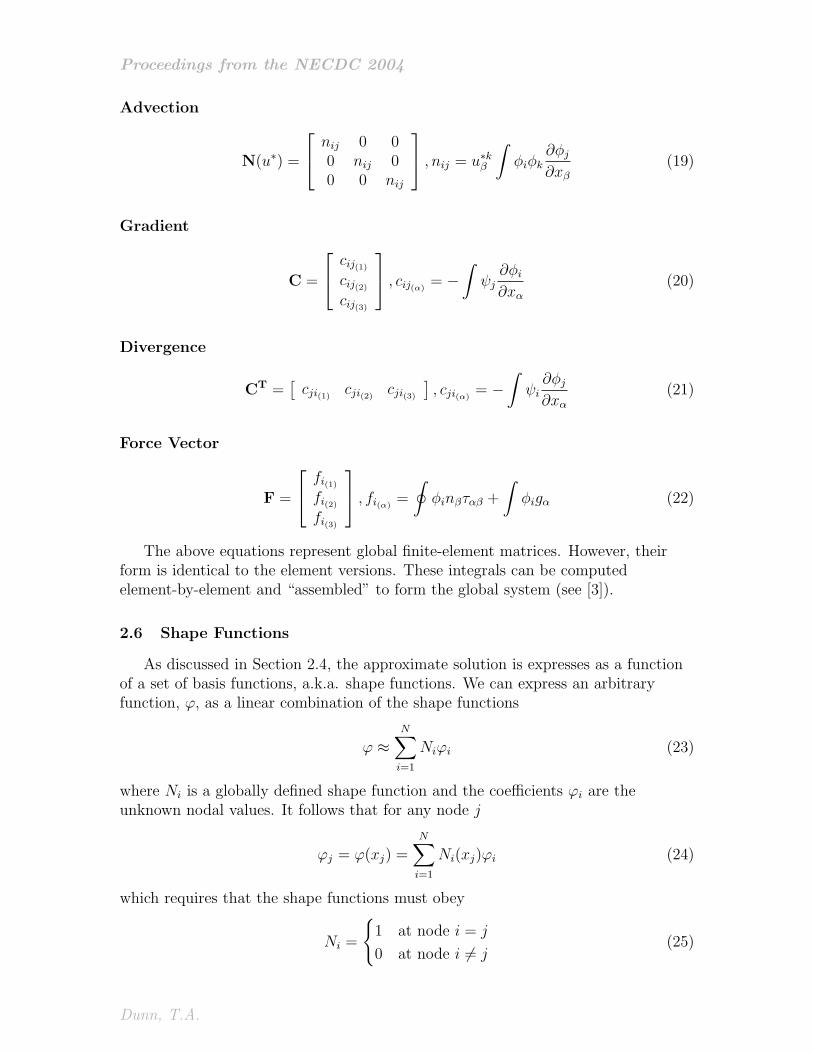
2.6 Shape Functions

As discussed in Section 2.4, the approximate solution is expresses as a functionof a set of basis functions, a.k.a. shape functions. We can express an arbitraryfunction, ϕ, as a linear combination of the shape functions

ϕ ≈N∑

i=1

Niϕi (23)

where Ni is a globally defined shape function and the coefficients ϕi are theunknown nodal values. It follows that for any node j

ϕj = ϕ(xj) =N∑

i=1

Ni(xj)ϕi (24)

which requires that the shape functions must obey

Ni =

1 at node i = j

0 at node i 6= j(25)

Dunn, T.A.


This implies the following identities:

N∑i=1

Ni = 1

N∑i=1

Nixi = x

N∑i=1

Niyi = y

(26)

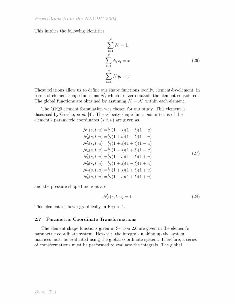
These relations allow us to define our shape functions locally, element-by-element, interms of element shape functions N , which are zero outside the element considered.The global functions are obtained by assuming Ni = Ni within each element.

The Q1Q0 element formulation was chosen for our study. This element isdiscussed by Gresho, et.al. [4]. The velocity shape functions in terms of theelement’s parametric coordinates (s, t, u) are given as

N1(s, t, u) =1/8(1− s)(1− t)(1− u)

N2(s, t, u) =1/8(1 + s)(1− t)(1− u)

N3(s, t, u) =1/8(1 + s)(1 + t)(1− u)

N4(s, t, u) =1/8(1− s)(1 + t)(1− u)

N5(s, t, u) =1/8(1− s)(1− t)(1 + u)

N6(s, t, u) =1/8(1 + s)(1− t)(1 + u)

N7(s, t, u) =1/8(1 + s)(1 + t)(1 + u)

N8(s, t, u) =1/8(1− s)(1 + t)(1 + u)

(27)

and the pressure shape functions are

NP (s, t, u) = 1 (28)

This element is shown graphically in Figure 1.

2.7 Parametric Coordinate Transformations

The element shape functions given in Section 2.6 are given in the element’sparametric coordinate system. However, the integrals making up the systemmatrices must be evaluated using the global coordinate system. Therefore, a seriesof transformations must be performed to evaluate the integrals. The global

Dunn, T.A.


Figure 1: Node numbering of element in local coordinates.

coordinates can be expressed in terms of the parametric coordinates as

x(s, t, u) =ne∑i=1

Ni(s, t, u)xi

y(s, t, u) =ne∑i=1

Ni(s, t, u)yi

z(s, t, u) =ne∑i=1

Ni(s, t, u)zi

(29)

whereNi(s, t, u) = Ni [x(s, t, u), y(s, t, u), z(s, t, u)]

Therefore, the derivatives of the shape functions can be expressed using the chainrule as

∂Ni

∂s=∂Ni

∂x

∂x

∂s+∂Ni

∂y

∂y

∂s+∂Ni

∂z

∂z

∂s∂Ni

∂t=∂Ni

∂x

∂x

∂t+∂Ni

∂y

∂y

∂t+∂Ni

∂z

∂z

∂t∂Ni

∂u=∂Ni

∂x

∂x

∂u+∂Ni

∂y

∂y

∂u+∂Ni

∂z

∂z

∂u

(30)

or equivalently in matrix form as ∂Ni

∂s∂Ni

∂t∂Ni

∂u

=

∂x∂s

∂y∂s

∂z∂s

∂x∂t

∂y∂t

∂z∂t

∂x∂u

∂y∂u

∂z∂u

∂Ni

∂x∂Ni

∂y∂Ni

∂z

= J

∂Ni

∂x∂Ni

∂y∂Ni

∂z

(31)

where J is the Jacobian matrix. The Jacobian matrix can be expressed asderivatives of the element shape functions

Jαβ =∂xα

∂sβ

=ne∑i=1

∂Ni(s, t, u)

∂sβ

xα,i (32)

Dunn, T.A.


The shape function derivatives in terms of the global coordinate system can becomputed using the inverse of the Jacobian matrix ∂Ni

∂x∂Ni

∂y∂Ni

∂z

= J−1

∂Ni

∂s∂Ni

∂t∂Ni

∂u

(33)

These values can then be used to evaluate the integrals in the matrix equations.From Calculus we know that the determinant of the Jacobian matrix can be used totransform an integral from one coordinate system to another using the relation

dΩ = dx dy dz = detJ ds dt du

Therefore, the matrix integrals can be evaluated with the transformation∫Ωe

ϕdΩ =

∫Ωe

ϕ(x, y, z) dx dy dz

=

∫ 1

−1

∫ 1

−1

∫ 1

−1

ϕ(s, t, u) detJ ds dt du

(34)

These integrals are then evaluated using Gaussian quadrature as described byComini [3]. Typically eight quadrature points are used. Single-point integration isalso useful, but requires hour-glass stabilization as discussed in Goudreau andHallquist [5].

2.8 Time-stepping Algorithm

Eqn. 16 represents a system of ordinary differential equations which must besolved in time. This presents a challenge, as this system is very difficult to solveefficiently in its coupled form. Therefore, we use a segregated solve to obtain thevelocity and pressure solutions in separate steps. In particular, we use an implicitprojection method to discretize the ODEs. This procedure is described in Gresho,et.al. [6]. The philosophy behind projection methods is to provide a way to decouplethe pressure and velocity fields to provide an efficient computational method tosolve transient incompressible flow problems.

First the momentum equation is discretized using a two-level split-thetatime-stepping scheme

[M + ∆tθKK + ∆tθNN(u∗)]u

∆t=

Mun

∆t− (1− θK)Kun − (1− θN)N(u∗n)un + Fn −MML

−1CP n

(35)

This equation is solved for an intermediate velocity u which does not satisfy thedivergence-free condition in the continuity equation. The value of the θs can bechosen to tailor your time-stepping scheme. Use θ = 0 for an explicit forward-Eulerscheme, θ = 1 for implicit backward-Euler, or θ = 1/2 for Crank-Nicholson. The

Dunn, T.A.


right-hand-side of this equation is computed using the pressure from the previoustime-step and the non-linear advection term is computed using a linearized guess forthe new velocity

u∗ = un + (∆t)∂un

∂t+ · · ·

For all results presented here, a zeroth-order approximation is used such that

u∗ = un

After we implicitly move the material with the momentum equation, the discretepressure-Poisson equation (PPE) is solved to enforce the continuity equation.[

CTML−1C− S

]λ = CT u

∆t

= CTML−1ML

u

∆t

(36)

where λ is a Lagrange multiplier used to update the pressure. ML is the lumpedmass matrix and S is a stabilization matrix used to remove spurious pressuremodes [7]. Note that multiplying the lumped mass matrix by its inverse on theright-hand-side is done purely for computational reasons to enforce boundaryconditions. We end the step by computing the final values of the pressure andvelocity

λ = P n+1 − P n ⇒ P n+1 = λ+ P n

un+1 = ∆tML−1

(ML

u

∆t−Cλ

)(37)

3 Solid Methodology

The implicit structural mechanics algorithm for solid materials is based on anupdated Lagrangian formulation. Dynamic equilibrium is obtained by solving a setof non-linear equations using the state and configuration at the end of thetime-step. Non-linearities arise due to material response and configuration changes.The method handles these non-linearities using a Newton-Raphson iteration toobtain the final configuration.

The local dynamic equilibrium relation is given by

ρuα =∂σαβ

∂xβ

+ ρbα (38)

where σ is the stress tensor, b is a body force vector per unit mass, ρ is the density,and u is the second time derivative of the nodal displacement vector. The principleof virtual work is used to obtain a weak form of the equation and the finite-elementmethod is used to discretize and solve the equation. This analysis can be found inthe report by Becker [8] and will not be repeated here as its derivation was not thefocus of the current project.

Dunn, T.A.


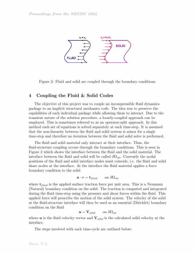
Figure 2: Fluid and solid are coupled through the boundary conditions.

4 Coupling the Fluid & Solid Codes

The objective of this project was to couple an incompressible fluid dynamicspackage to an implicit structural mechanics code. The idea was to preserve thecapabilities of each individual package while allowing them to interact. Due to thetransient nature of the solution procedure, a loosely-coupled approach can beemployed. This is sometimes referred to as an operator-split approach. In thismethod each set of equations is solved separately at each time-step. It is assumedthat the non-linearity between the fluid and solid system is minor for a singletime-step and therefore no iteration between the fluid and solid solve is performed.

The fluid and solid material only interact at their interface. Thus, thefluid-structure coupling occurs through the boundary conditions. This is seen inFigure 2 which shows the interface between the fluid and the solid material. Theinterface between the fluid and solid will be called ∂Ωint. Currently the nodalpositions of the fluid and solid interface nodes must coincide, i.e. the fluid and solidshare nodes at the interface. At the interface the fluid material applies a forceboundary condition to the solid

n · σ = tfluid on ∂Ωint

where tfluid is the applied surface traction force per unit area. This is a Neumann(Natural) boundary condition on the solid. The traction is computed and integratedduring the fluid time-step using the pressure and shear forces within the fluid. Thisapplied force will prescribe the motion of the solid system. The velocity of the solidat the fluid-structure interface will then be used as an essential (Dirichlet) boundarycondition on the fluid

u = Vsolid on ∂Ωint

where u is the fluid velocity vector and Vsolid is the calculated solid velocity at theinterface.

The steps involved with each time-cycle are outlined below:

Dunn, T.A.


1. Solid Solution

• Solve for new solid configuration (using force obtained during previousfluid cycle)

• Solve for velocity at the interface

2. Mesh Relaxation

• Move fluid grid to account for new solid configuration

• Compute grid velocity based on change in grid position

• Advect fluid variables (Advection Option #2 Only)

3. Fluid Solution

• Solve for fluid velocity and pressure

• Compute force acting on interface

4. Complete the Cycle

• Post-Process

• Increment Time

• Return To Step 1

5 Results

Two test cases were run for this project. The first test looked at flow around arigid sphere with a moving grid. This test was designed to validate the grid motioncapability of the incompressible flow model. Therefore, the solid mechanics codewas not utilized for this test. The second test also looked at flow around a movingsphere, but the sphere was solid and it’s motion was computed by the solidmechanics code.

5.1 Test Case #1: Flow Around a Sphere

Test problem #1 looked at flow around a three-dimensional circular sphere. Inthis case the sphere was rigid and the flow conditions were

D = 1 Diameter of SphereUinf = 1 Freestream Velocityν = 0.1 Kinematic Viscosity⇒ Re = 10 Reynolds Number

At a Reynolds Number of 10, the flow has not yet separated but the streamlines areasymmetric (see Van Dyke [9]). In order to test the grid motion, this test was runon a fixed grid with a uniform freestream velocity and on a moving grid where the

Dunn, T.A.


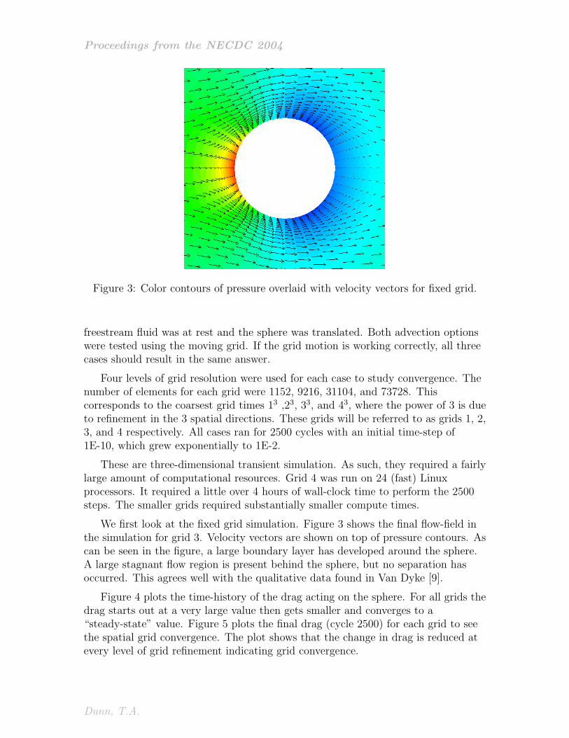
Figure 3: Color contours of pressure overlaid with velocity vectors for fixed grid.

freestream fluid was at rest and the sphere was translated. Both advection optionswere tested using the moving grid. If the grid motion is working correctly, all threecases should result in the same answer.

Four levels of grid resolution were used for each case to study convergence. Thenumber of elements for each grid were 1152, 9216, 31104, and 73728. Thiscorresponds to the coarsest grid times 13 ,23, 33, and 43, where the power of 3 is dueto refinement in the 3 spatial directions. These grids will be referred to as grids 1, 2,3, and 4 respectively. All cases ran for 2500 cycles with an initial time-step of1E-10, which grew exponentially to 1E-2.

These are three-dimensional transient simulation. As such, they required a fairlylarge amount of computational resources. Grid 4 was run on 24 (fast) Linuxprocessors. It required a little over 4 hours of wall-clock time to perform the 2500steps. The smaller grids required substantially smaller compute times.

We first look at the fixed grid simulation. Figure 3 shows the final flow-field inthe simulation for grid 3. Velocity vectors are shown on top of pressure contours. Ascan be seen in the figure, a large boundary layer has developed around the sphere.A large stagnant flow region is present behind the sphere, but no separation hasoccurred. This agrees well with the qualitative data found in Van Dyke [9].

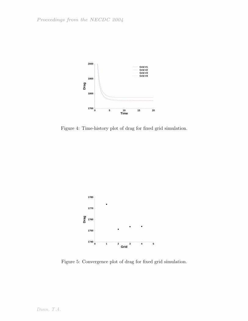
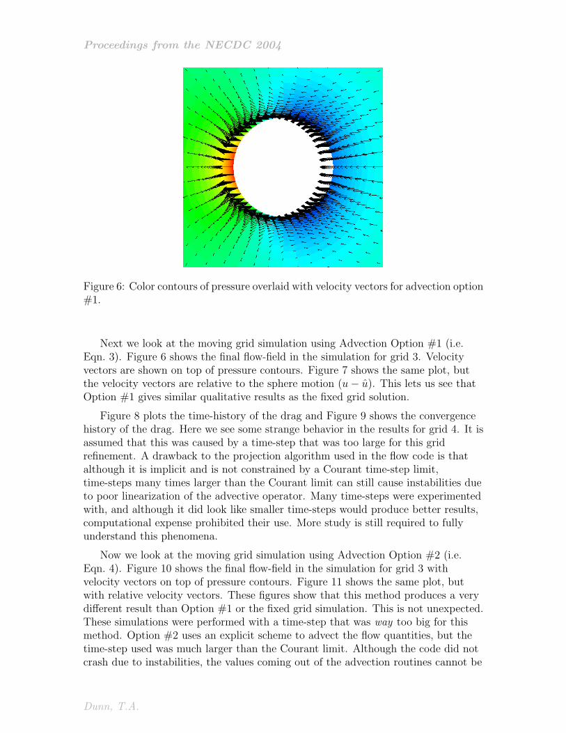
Figure 4 plots the time-history of the drag acting on the sphere. For all grids thedrag starts out at a very large value then gets smaller and converges to a“steady-state” value. Figure 5 plots the final drag (cycle 2500) for each grid to seethe spatial grid convergence. The plot shows that the change in drag is reduced atevery level of grid refinement indicating grid convergence.

Dunn, T.A.


0 5 10 15 20Time

1700

1800

1900

2000

Dra

g

Grid #1Grid #2Grid #3Grid #4

Figure 4: Time-history plot of drag for fixed grid simulation.

0 1 2 3 4 5Grid

1740

1750

1760

1770

1780

Dra

g

Figure 5: Convergence plot of drag for fixed grid simulation.

Dunn, T.A.


Figure 6: Color contours of pressure overlaid with velocity vectors for advection option#1.

Next we look at the moving grid simulation using Advection Option #1 (i.e.Eqn. 3). Figure 6 shows the final flow-field in the simulation for grid 3. Velocityvectors are shown on top of pressure contours. Figure 7 shows the same plot, butthe velocity vectors are relative to the sphere motion (u− u). This lets us see thatOption #1 gives similar qualitative results as the fixed grid solution.

Figure 8 plots the time-history of the drag and Figure 9 shows the convergencehistory of the drag. Here we see some strange behavior in the results for grid 4. It isassumed that this was caused by a time-step that was too large for this gridrefinement. A drawback to the projection algorithm used in the flow code is thatalthough it is implicit and is not constrained by a Courant time-step limit,time-steps many times larger than the Courant limit can still cause instabilities dueto poor linearization of the advective operator. Many time-steps were experimentedwith, and although it did look like smaller time-steps would produce better results,computational expense prohibited their use. More study is still required to fullyunderstand this phenomena.

Now we look at the moving grid simulation using Advection Option #2 (i.e.Eqn. 4). Figure 10 shows the final flow-field in the simulation for grid 3 withvelocity vectors on top of pressure contours. Figure 11 shows the same plot, butwith relative velocity vectors. These figures show that this method produces a verydifferent result than Option #1 or the fixed grid simulation. This is not unexpected.These simulations were performed with a time-step that was way too big for thismethod. Option #2 uses an explicit scheme to advect the flow quantities, but thetime-step used was much larger than the Courant limit. Although the code did notcrash due to instabilities, the values coming out of the advection routines cannot be

Dunn, T.A.


Figure 7: Color contours of pressure overlaid with relative velocity vectors for ad-vection option #1.

0 5 10 15 20Time

1700

1800

1900

2000

Dra

g


Figure 8: Time-history plot of drag for advection option #1 simulation.

Dunn, T.A.


0 1 2 3 4 5Grid

1700

1800

1900

Dra

g

Figure 9: Convergence plot of drag for advection option #1 simulation.

Figure 10: Color contours of pressure overlaid with velocity vectors for advectionoption #2.

Dunn, T.A.


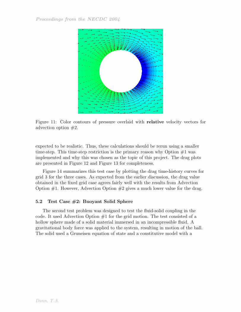
Figure 11: Color contours of pressure overlaid with relative velocity vectors foradvection option #2.

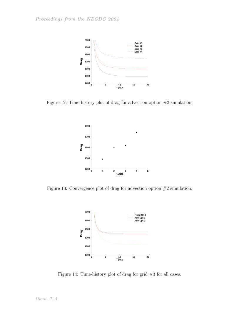
expected to be realistic. Thus, these calculations should be rerun using a smallertime-step. This time-step restriction is the primary reason why Option #1 wasimplemented and why this was chosen as the topic of this project. The drag plotsare presented in Figure 12 and Figure 13 for completeness.

Figure 14 summarizes this test case by plotting the drag time-history curves forgrid 3 for the three cases. As expected from the earlier discussion, the drag valueobtained in the fixed grid case agrees fairly well with the results from AdvectionOption #1. However, Advection Option #2 gives a much lower value for the drag.

5.2 Test Case #2: Buoyant Solid Sphere

The second test problem was designed to test the fluid-solid coupling in thecode. It used Advection Option #1 for the grid motion. The test consisted of ahollow sphere made of a solid material immersed in an incompressible fluid. Agravitational body force was applied to the system, resulting in motion of the ball.The solid used a Gruneisen equation of state and a constitutive model with a

Dunn, T.A.


0 5 10 15 20Time

1400

1500

1600

1700

1800

1900

2000

Dra

g


Figure 12: Time-history plot of drag for advection option #2 simulation.

0 1 2 3 4 5Grid

1400

1500

1600

1700

1800

Dra

g

Figure 13: Convergence plot of drag for advection option #2 simulation.

0 5 10 15 20Time

1500

1600

1700

1800

1900

2000

Dra

g

Fixed GridAdv Opt 1Adv Opt 2

Figure 14: Time-history plot of drag for grid #3 for all cases.

Dunn, T.A.


Figure 15: Initial Configuration and Hydrostatic Pressure

constant shear modulus. The following parameters were used:

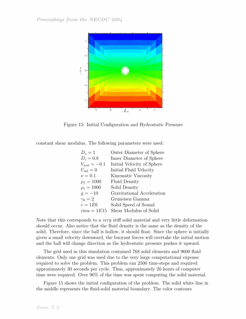
Do = 1 Outer Diameter of SphereDi = 0.8 Inner Diameter of SphereVinit = −0.1 Initial Velocity of SphereUinf = 0 Initial Fluid Velocityν = 0.1 Kinematic Viscosityρf = 1000 Fluid Densityρs = 1000 Solid Densityg = −10 Gravitational Accelerationγ0 = 2 Gruneisen Gammac = 1E6 Solid Speed of Soundcmu = 1E15 Shear Modulus of Solid

Note that this corresponds to a very stiff solid material and very little deformationshould occur. Also notice that the fluid density is the same as the density of thesolid. Therefore, since the ball is hollow, it should float. Since the sphere is initiallygiven a small velocity downward, the buoyant forces will overtake the initial motionand the ball will change direction as the hydrostatic pressure pushes it upward.

The grid used in this simulation contained 768 solid elements and 9600 fluidelements. Only one grid was used due to the very large computational expenserequired to solve the problem. This problem ran 2500 time-steps and requiredapproximately 30 seconds per cycle. Thus, approximately 20 hours of computertime were required. Over 90% of the time was spent computing the solid material.

Figure 15 shows the initial configuration of the problem. The solid white line inthe middle represents the fluid-solid material boundary. The color contours

Dunn, T.A.


Figure 16: Initial Configuration and Flow Around Solid Ball

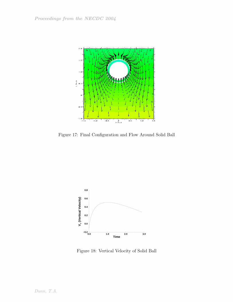
represent pressure. Notice that the fluid has established the hydrostatic pressurethroughout the solution. Figure 16 shows the same configuration, but zoomed in toview the ball. Fluid velocity vectors are also added to the plot. Notice that thevelocity vectors are initially pointing downward, following the motion of the ball.Figure 17 shows the final configuration of the simulation. At this point the ball hasan upward velocity and has moved a distance a little more than the ball diameter.The motion of the solid has started to cause the fluid to recirculate. The fluid nearthe solid boundary is moving upward with the ball. Away from the sphere, the fluidis rushing downward to fill in the gap left by the moving solid.

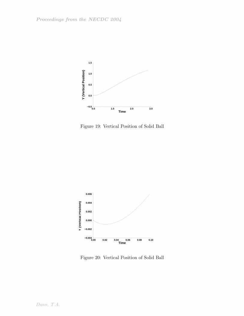
The next plots provide a time-history of the motion of the ball. Figure 18 showsthe vertical velocity of the sphere verses time. The sphere initially has a negativevelocity, but as the hydrostatic pressure in the fluid pushes the ball upward thevelocity increases. Towards the end of the simulation, drag begins to decelerate thesphere. It is unclear why the ball overshoots its terminal velocity. This will need tobe investigated with a grid convergence study. Figure 19 shows the ball’s positionverses time (Figure 20 provides a zoomed in look at the start-up). As discussed forthe velocity plot, the ball initially moves downward, then changes direction andmoves upward.

Without a formal validation and grid convergence study no conclusions can bedrawn to the accuracy of the method. However, the simulation does provide resultsthat are qualitatively similar to what would be expected.

Dunn, T.A.


Figure 17: Final Configuration and Flow Around Solid Ball

0.0 1.0 2.0 3.0Time

−0.2

0.0

0.2

0.4

0.6

0.8

VY (

Ver

tica

l Vel

oci

ty)

Figure 18: Vertical Velocity of Solid Ball

Dunn, T.A.


0.0 1.0 2.0 3.0Time

−0.5

0.0

0.5

1.0

1.5

Y (

Ver

tica

l Po

siti

on

)

Figure 19: Vertical Position of Solid Ball

0.00 0.02 0.04 0.06 0.08 0.10Time

−0.004

−0.002

0.000

0.002

0.004

0.006

Y (

Ver

tica

l Po

siti

on

)

Figure 20: Vertical Position of Solid Ball

Dunn, T.A.


6 Conclusions

An incompressible flow code was coupled to an implicit solids code to investigatefluid-structure interaction. In order to do this, the fluids code was modified to allowgrid motion using the ALE methodology. Two test cases were run: one to validatethe grid motion capability in the fluid code and a second to check the fluid-structurecoupling. A few conclusions are summarized here.

• Advection Option #1 was able to reasonably reproduce a fixed grid solutionusing a moving grid. Both agreed qualitatively with flow-field visualizationexperiments.

• Advection Option #2 did not predict the correct flow. It is assumed that thiswas caused by time-steps which were too large. This should be investigatedmore.

• The implicit projection method used for the fluid equations requires“reasonably” sized time-steps for accurate solutions. This could haveinfluenced the convergence study results.

• Test problem 1 should be investigated further with an analysis oftime-discretization effects.

• The code was able to provide some insight into the fluid-structure interactionfor a buoyant sphere.

• A more detailed grid-resolution study is required for test problem 2.

The following items may be considered for future projects to improve theperformance of the code:

• Non-linear iteration may be required for convergence between the fluid andsolid.

• Strong coupling may be required–solve both fluid and solid in the same matrixsolution.

• Iteration within the incompressible flow step to better address the non-linearadvective term could improve the projection algorithm.

This is an ongoing project. There is still plenty of work to be done.

Acknowledgments

This work was performed under the auspices of the U.S. Department of Energyby University of California, Lawrence Livermore National Laboratory underContract W-7405-Eng-48.

Dunn, T.A.


References

[1] Uchiyama T, ALE finite element method for gas-liquid two-phase flow includingmoving boundary based on an incompressible two-fluid model. NuclearEngineering and Design, 2001; 205:69–82.

[2] Benson DJ, Computational methods in Lagrangian and Eulerian hydrocodes.Computer Methods in Applied Mechanics and Engineering, 1992; 99:235–394.

[3] Comini G, Del Giudice S, Nonino C, Finite Element Analysis in Heat TransferBasic Formulation and Linear Problems, 1994, Taylor & Francis.

[4] Gresho PM, Chan ST, Lee RL, Upson CD. A modified finite element method forsolving the time-dependent, incompressible Navier-Stokes equations part 1:theory. International Journal for Numerical Methods in Fluids 1984;4(6):557–598.

[5] Goudreau GL, Hallquist JO. Recent developments in large-scale finite elementLagrangian hydrocode technology. Computational Methods in Applied Mechanicsand Engineering 1982; 33(1-3):725-757.

[6] Gresho PM, Chan ST, Projection 2 goes turbulent–and fully implicit.International Journal of Computational Fluid Dynamics, 1998; 9(3-4):249–272.

[7] Silvester DJ, Kechkar N, Stabilised bilinear-constant velocity-pressure finiteelements for the conjugate gradient solution of the Stokes problem. ComputerMethods in Applied Mechanics and Engineering, 1990; 79:71–86.

[8] Becker R, The implicithydro package in ALE3D. Unpublished Draft, 2004.

[9] Van Dyke M, An Album of Fluid Motion, 1982, The Parabolic Press.

Dunn, T.A.

ale method fsi

Documents

fluid motion

fluid flow problems

fluid equations

united states government

euler method

lagrange method

united statesoctober

university of california