algebraicity criteria and their applications
TRANSCRIPT
Algebraicity Criteria and Their ApplicationsThe Harvard community has made this
article openly available. Please share howthis access benefits you. Your story matters
Citation Tang, Yunqing. 2016. Algebraicity Criteria and Their Applications.Doctoral dissertation, Harvard University, Graduate School of Arts &Sciences.
Citable link http://nrs.harvard.edu/urn-3:HUL.InstRepos:33493480
Terms of Use This article was downloaded from Harvard University’s DASHrepository, and is made available under the terms and conditionsapplicable to Other Posted Material, as set forth at http://nrs.harvard.edu/urn-3:HUL.InstRepos:dash.current.terms-of-use#LAA

Algebraicity criteria and their applications
A dissertation presented
by
Yunqing Tang
to
The Department of Mathematics
in partial fulfillment of the requirementsfor the degree of
Doctor of Philosophyin the subject ofMathematics
Harvard UniversityCambridge, Massachusetts
May 2016

c 2016 – Yunqing TangAll rights reserved.

Dissertation Advisor: Professor Mark Kisin Yunqing Tang
Algebraicity criteria and their applications
Abstract
We use generalizations of the Borel–Dwork criterion to prove variants of the Grothedieck–Katz
p-curvature conjecture and the conjecture of Ogus for some classes of abelian varieties over number
fields.
The Grothendieck–Katz p-curvature conjecture predicts that an arithmetic differential equation
whose reduction modulo p has vanishing p-curvatures for all but finitely many primes p, has finite
monodromy. It is known that it suffices to prove the conjecture for differential equations on P1 −
0, 1,∞. We prove a variant of this conjecture for P1−0, 1,∞, which asserts that if the equation
satisfies a certain convergence condition for all p, then its monodromy is trivial. For those p for
which the p-curvature makes sense, its vanishing implies our condition. We deduce from this a
description of the differential Galois group of the equation in terms of p-curvatures and certain
local monodromy groups. We also prove similar variants of the p-curvature conjecture for a certain
elliptic curve with j-invariant 1728 minus its identity and for P1 − ±1,±i,∞.
Ogus defined a class of cycles in the de Rham cohomology of smooth proper varieties over number
fields. This notion is a crystalline analogue of -adic Tate cycles. In the case of abelian varieties,
this class includes all the Hodge cycles by the work of Deligne, Ogus, and Blasius. Ogus predicted
that such cycles coincide with Hodge cycles for abelian varieties. We confirm Ogus’ conjecture for
some classes of abelian varieties, under the assumption that these cycles lie in the Betti cohomology
with real coefficients. These classes include abelian varieties of prime dimension that have nontrivial
endomorphism ring. The proof uses a crystalline analogue of Faltings’ isogeny theorem due to Bost
and the known cases of the Mumford–Tate conjecture. We also discuss some strengthenings of the
theorem of Bost.
iii

Contents
Acknowledgements v
Chapter 1. Introduction 1
The Grothendieck–Katz p-curvature conjecture 2
The conjecture of Ogus 3
A relative version of Bost’s theorem 6
Chapter 2. Algebraicity criteria 8
1. Formal power series 8
2. Formal subschemes 11
Chapter 3. Grothendieck–Katz p-curvature conjecture 19
3. Statement of the main results 20
4. The proof: an application of theorems due to André and Bost–Chambert-Loir 26
5. Interpretation using the Faltings height 32
6. The affine elliptic curve case and examples 38
Chapter 4. The conjecture of Ogus 44
7. De Rham–Tate cycles and a result of Bost 45
8. Frobenius Tori and the Mumford–Tate conjecture 53
9. Proof of the main theorem 64
Chapter 5. A relative version of Bost’s theorem 73
10. The known cases 73
11. A strengthening of Theorem 7.3.7 and its application 75
Bibliography 80
iv
Acknowledgements
I thank my advisor Mark Kisin for introducing these problems to me and for all the enlight-
ening discussions and encouragement. I thank Yves André, Noam Elkies, Hélène Esnault, and
Benedict Gross for useful comments. I thank George Boxer,Victoria Cantoral-Farfán, Kęstutis Čes-
navičius, Erick Knight, Chao Li, Yifeng Liu, Andreas Maurischat, Barry Mazur, Curtis McMullen,
Ananth Shankar, Koji Shimizu, Junecue Suh, Cheng-Chiang Tsai, Jerry Wang, Shou-wu Zhang,
Yihang Zhu for helpful discussions or/and remarks on previous drafts on these results. I thank
Harvard math department as a fantastic place for my graduate study and research. In addition
to the above list, I thank Gabriel Bujokas, Hansheng Diao, Mboyo Esole, Jessica Fintzen, Bao Le
Hung, Tom Lovering, Yong Suk Moon, Anand Patel, Pei-Yu Tsai, Carl Wang Erickson, Rong Zhou
and other members of the math department for mathematics and related conversations. I thank
Susan Gilbert, who has been supportive on all administrative related things. I thank my family for
always being supportive.
v

CHAPTER 1
Introduction
Many problems in arithmetic geometry concern the existence of certain algebraic cycles or
subvarieties and one strategy to prove such existence is to construct analytic objects first and then
to develop suitable criteria which use arithmetic properties to show the algebraicity. These criteria
are originated from the classical Borel–Dwork criterion, which asserts that a nice formal power series
with rational coefficients is the power series expansion of a rational function if the product of its
convergence radii at all places is larger than 1. Here by a nice power series, we mean that the set
of primes dividing some of the denominators of the coefficients is finite. Dwork used this criterion
to prove that the zeta function of a smooth projective variety over a finite field is rational, which
was part of the Weil conjectures.
Informally speaking, generalizations of the Borel–Dwork criterion concern the algebraicity of
analytic subvarieties of smooth algebraic varieties defined over number fields. There are many
instances in arithmetic geometry where the algebraicity of certain analytic subvarieties is desired,
as illustrated in the following examples.
The first example is the Grothendieck–Katz p-curvature conjecture, which concerns vector bun-
dles with flat connections. This conjecture is a local-global principle of the algebraicity of the
solutions of an arithmetic linear homogenous differential equation. The p-curvature is an invariant
of the differential equation modulo p and its vanishing is equivalent to the existence of a full set of
mod p rational solutions. Under the assumption of the vanishing of p-curvatures for all but finitely
primes, one needs to show the algebraicity of the formal solutions of the differential equation.
The second example is a conjecture of Ogus, which is a crystalline analogue of the Mumford–
Tate conjecture. Ogus defined absolute Tate cycles using the structure of de Rham and crystalline
cohomologies and conjectured that these cycles coincide with Hodge cycles. A variant of Ogus’
conjecture for abelian varieties over number fields would follow from the conjectural algebraicity of
certain formal subschemes of the moduli space of principally polarized abelian varieties.
We use generalizations of the Borel–Dwork criterion (see chapter 2) to prove:
1

(1) Variants of the Grothedieck–Katz p-curvature conjecture under the assumption of vanishing
p-curvature at all primes (see chapter 3);
(2) The conjecture of Ogus for some classes of abelian varieties over number fields under the
assumption that all absolute Tate cycles lie in Betti cohomology with real coefficients (see
chapter 4).
In chapter 5, we discuss a conjecture arising naturally from our study of the conjecture of Ogus.
The Grothendieck–Katz p-curvature conjecture
Let X be a smooth variety over a number field K and (M,∇) a vector bundle with a flat
connection over X. The Grothendieck–Katz p-curvature conjecture predicts that (M,∇) has finite
monodromy if and only if, for all but finitely many primes p, (M,∇) modulo p has vanishing p-
curvature. It is known that it suffices to prove the conjecture when X = P1K − 0, 1,∞. We prove
a variant of the conjecture for X = P1K − 0, 1,∞ where the condition for all but finitely many p
is replaced by a condition for all p. A slightly informal formulation of our result is the following:
Theorem 1 (Theorem 3.2.1). Let (M,∇) be a vector bundle with a connection over X = P1K −
0, 1,∞. If the p-curvature of (M,∇) vanishes for all p, then (M,∇) is trivial, that is, M∇=0
generates M as an OX-module.
Let us explain the meaning of the condition of vanishing p-curvature at all primes p: at primes
where the p-curvature is either not defined or non-vanishing, we impose a condition on the p-adic
radii of convergence of the horizontal sections of (M,∇). When (M,∇) has an integral model at a
prime p so that one can make sense of its reduction mod p, this convergence condition is implied
by the vanishing of the p-curvature.
One can extend the notion of vanishing p-curvature for all p to vector bundles with connections
over smooth algebraic curves equipped with either a semistable model over OK or a flat model over
OK with a smooth OK-point. However, the property of all p-curvatures vanishing is not preserved
under push-forward along finite maps from the curve in question to P1 − 0, 1,∞. Therefore, one
cannot deduce from Theorem 1 that vanishing p-curvature for all p implies trivial monodromy in
the case of arbitrary algebraic curves. Nevertheless, when X is an elliptic curve with j-invariant
1728 minus its identity point, we prove:2

Theorem 2 (Theorem 6.1.1). Let X ⊂ A2Zbe the affine curve defined by y
2 = x(x− 1)(x+ 1) and
let (M,∇) be a vector bundle with a connection over XK . If the p-curvature of (M,∇) vanishes for
all p, then (M,∇) has finite monodromy. That is, there exists a finite étale morphism f : Y → X
such that f∗(M,∇) is trivial.
Unlike in Theorem 1, passing to a finite étale cover is necessary. In the setting of Theorem 2,
there is an example of an (M,∇) with monodromy group equal to Z/2Z.
The main tools used to prove Theorem 1 and Theorem 2 are the algebraicity results of André
[And04a, Thm. 5.4.3] and Bost–Chambert-Loir [BCL09, Thm. 6.1, Thm. 7.8]. André and Bost
used these techniques to prove the p-curvature conjecture when one knows a priori that the mon-
odromy group of (M,∇) is solvable. Our estimates of archimedean radii use the properties of theta
functions, the Chowla–Selberg formula, and works of Hempel [Hem79] and Eremenko [Ere11].
The conjecture of Ogus
The Mumford–Tate conjecture asserts that, via the Betti–étale comparison isomorphism, the Q-
linear combinations of Hodge cycles coincide with the -adic Tate cycles. As a crystalline analogue,
Ogus defined the notion of absolute Tate cycles for any smooth projective variety X over a number
field K and predicted that for any embedding σ : K → C, via the de Rham–Betti comparison
isomorphism
cBdR : H iB(Xσ(C),Q)⊗Q C ∼= H
idR(X/K)⊗K,σ C,
absolute Tate cycles coincide with absolute Hodge cycles ([Ogu82, Hope 4.11.3]). For any finite
extension L of K, an element in the tensor algebra of
2 dimXi=0 H
idR(X/K)⊗ L
is called an absolute Tate cycle if it is fixed by all but finitely many crystalline Frobenii ϕv. When
v is unramified, ϕv can be viewed as acting on HidR(X/K) ⊗ Kv via the canonical isomorphism
between de Rham and crystalline cohomologies.
Ogus proved that all Hodge cycles are absolute Tate for abelian varieties and verified the agree-
ment of absolute Hodge cycles and absolute Tate cycles when X is a product of abelian varieties
with complex multiplication, Fermat hypersurfaces, and projective spaces ([Ogu82, Thm. 4.16]).3

It is natural to take the archimedean places into account: complex conjugation on the Betti
cohomology can be viewed as the analogue of the Frobenii acting on the crystalline cohomology.
We define the de Rham–Tate cycles to be those absolute Tate cycles which, for any embedding
σ : K → C, lie in the tensor algebra of
cBdR(2 dimX
i=0 HiB(Xσ(C),Q)⊗Q R).
Our first result is the following:
Theorem 3 (Theorem 8.2.4). If A is a polarized abelian variety over Q and its -adic algebraic
monodromy group G is connected, then the Mumford–Tate conjecture for A implies that the de
Rham–Tate cycles coincide with the Hodge cycles.
The Mumford–Tate conjecture for abelian varieties is known in many cases. When the abelian
variety A over K satisfies EndK(A) = Z, Pink proved that the conjecture holds when 2 dimA is not
in the set ([Pin98])
SPink = a2b+1,
4b+ 2
2b+ 1
|a, b ∈ N\0.
To show this, he constructed a Q-model of G
which is independent of and “looks like” the
Mumford–Tate group GMT in the following sense. The group GMT (resp. the Q-model of G
)
with its tautological faithful absolutely irreducible representation H1B(A,Q) (resp. H1
ét(AK ,Q)) is
an (absolutely) irreducible strong Mumford–Tate pair over Q: the group is reductive and generated
over Q by the image of a cocharacter of weights (0, 1). Based on the work of Serre, Pink gave a
classification of irreducible Mumford–Tate pairs; see [Pin98, Prop. 4.4, 4.5, and Table 4.6]. This
classification unconditionally shows that G is of a very restricted form.
In the crystalline setting, we define the de Rham–Tate group GdR of a polarized abelian variety
A over K to be the algebraic subgroup of GL(H1dR(A/K)) stabilizing all of the de Rham–Tate
cycles. This group is reductive by our assumption that de Rham–Tate cycles are fixed by complex
conjugation. We show that Pink’s classification also applies to GdR in the following situation:
Theorem 4 (Theorem 8.2.6). Let A be a polarized abelian variety over Q and assume that its -adic
algebraic monodromy group is connected. If EndQ(A) = Z, then the neutral connected component of
GdR with its tautological representation is an irreducible strong Mumford–Tate pair over Q.
4

A key input to the proofs of both theorems is:
Proposition 5. Let M be a set of rational primes of natural density one and let A be a polarized
abelian variety over K. If s ∈ End(H1dR(A/K) ⊗ L) satisfies that ϕv(s) = s for all v lying over
some p ∈ M , then s comes from an algebraic cycle over L.
Bost proved such algebraicity of s assuming ϕv(s) = s for all but finitely many v ([Bos06,
Thm. 6.4]). Both results may be viewed as analogues of Faltings’ isogeny theorem. Based on Bost’s
work, on [Gas10], and on [Her12], we prove a strengthening (Corollary 11.1.2, Remark 11.1.3)
only assume the density of M to be strictly larger than 1 − 12(dimA+1) for general A or 3/4 for A
absolutely simple.
Before we present a result valid for a general number field K, we explain the main difficulty
in going beyond the K = Q case in Theorem 3 and Theorem 4. For simplicity, we focus on
the case when EndK(A) = Z. Pink’s classification applies to connected reductive groups with an
absolutely irreducible representation. Though we can deduce the irreducibility of H1dR(A/K) as
a GdR-representation from Bost’s theorem, GdR is a priori not known to be connected. In the
-adic setting, Serre, using the Chebotarev density theorem, showed that G will be connected after
passing to a finite extension ([Ser13]). There seems to be no easily available analogous argument
for GdR. However, when K = Q, the absolute Frobenii coincide with the relative ones. Thus the
connectedness of G implies that GdR is almost connected: ϕp ∈ G
dR(Qp) for all p in a set of natural
density 1. In other words, although one cannot prove directly that elements fixed by G
dR are de
Rham–Tate cycles, such elements are fixed by ϕp for all p in a density one set.
Beyond the K = Q case, we have proved the following result.
Theorem 6. Let A be an abelian variety over some number field such that it is isogenous to
ni=1A
ni
i , where Ai is absolutely simple and Ai is not isogenous to Aj over any number field for
i = j. Assume that each Ai is one of the following cases:
(1) Ai is an elliptic curve or has complex multiplication.
(2) The dimension of Ai is a prime number and EndK(Ai) is not Z.
(3) The polarized abelian variety Ai of dimension g with EndK(Ai) = Z is defined over a finite
Galois extension K over Q such that [K : Q] is prime to g! and 2g /∈ SPink.
5

and that if there is an Ai of case (2) with EndK(Ai)⊗Q being an imaginary quadratic field, then all
the other Aj are not of type IV. Then the de Rham–Tate cycles of A coincide with its Hodge cycles.
Case (1) was known before our work: Ogus proved the case of abelian varieties with complex
multiplication and the case of elliptic curves is a direct consequence of the Serre–Tate theory. For
the rest, the main task is to show that the centralizer of G
dR in End(H1dR(A/K)) coincides with that
of GdR. In case (2), since the Mumford–Tate group is not too large, we use Bost’s theorem to show
that otherwise G
dR must be a torus. Then we deduce that A must have complex multiplication
by a theorem of Noot ([Noo96, Thm. 2.8]) on formal deformation spaces at a point of ordinary
reduction and hence we reduce this case to case (1). To exploit Proposition 5 to tackle case (3), we
need to understand ϕv for all v lying over p ∈ M , where M is a set of rational primes of natural
density 1. While Serre’s theorem on the ranks of Frobenius tori only provides information about
completely split primes, we prove a refinement when G = GSp2g that takes into account the other
primes. This refinement asserts that the Frobenius tori are of maximal rank for all v lying over
p ∈ M . The rest of the argument is similar to that of case (2). In order to prove the result for the
product of abelian varieties in these three cases, we record a proof of the Mumford–Tate conjecture
for abelian varieties studied in the theorem following the idea of [Lom15].
A relative version of Bost’s theorem
In the description of -adic Tate cycles over some number field L, one uses relative Frobenii in-
stead of the absolute ones. It is natural to use relative Frobenii acting on the crystalline cohomology
to define an analogous notion of absolute Tate cycles (see Definition 10.1.1). In analogy with the
Mumford–Tate conjecture and the conjecture of Ogus, one may expect that such cycles are L-linear
combinations of the absolute Hodge cycles. In particular, we expect the following counterpart of
Bost’s theorem (see Proposition 5) for an abelian variety A over a number field K.
Conjecture 7. Let L be a finite extension of K and for any finite place v with residue characteristic
p, write mv = [Lv : Qp]. If s ∈ End(H1dR(AL/L)) is fixed by all but finitely many relative Frobenii
ϕmv
v , then s is an L-linear combination of algebraic cycles.
6
The validity of this conjecture implies that the agreement of de Rham–Tate cycles and Hodge
cycles is a consequence of the Mumford–Tate conjecture, generalizing Theorem 3. The full validity
of this conjecture seems difficult. Nevertheless, we prove
Theorem 8 (section 10.2). Conjecture 7 is valid when A is an elliptic curve, has complex multipli-
cation, or is an abelian surface with quaternion multiplication.
Notation and convention. Let K be a number field and OK its ring of integers. For a place
v of K, either archimedean or finite, let Kv be the completion of K with respect to v. When v is
finite, we denote by p, Ov, and kv the corresponding prime ideal, the ring of integers, and residue
field of Kv. We also denote by pv the characteristic of kv and when there is no confusion, we will
also write p for pv. When we say all places or any place v of K, this v can be both archimedean
and finite. If there is no specific indication, L denotes a finite extension of K.
For any vector space or vector bundle V , let V∨ be its dual and we denote V
⊗m ⊗ (V ∨)⊗n
by Vm,n. For a vector space V , we use GL(V ),GSp(V ), . . . to denote the algebraic groups rather
than the rational points of these algebraic groups. For any scheme X or vector bundle/space V
over Spec(R), we denote by XR or V
R the base change to SpecR for any R-algebra R
. For any
archimedean place σ of K and any variety X over K, we use Xσ to denote the base change of X to
C via a corresponding embedding σ : K → C.
A reductive algebraic group here could be nonconnected.
Given an algebraic group G, we use G to denote its neutral connected component and use Z(G)
to denote its center. We use Z(G) to denote the connected component of Z(G).
For any field F , we use F to denote a chosen algebraic closure of F . For any finite dimensional
vector space V over F and any subset S of V , we use SpanF (S) to denote the smallest sub F -vector
space of V containing S.
For an Hermitian vector bundle E over an OK-scheme X, we may use E to denote both the
vector bundle over X and that over XK . If necessary, we may use E and E to distinguish the one
over X and the one over XK .
7

CHAPTER 2
Algebraicity criteria
In section 1, we state results on formal power series by André and Bost–Chambert-Loir which
will be used in chapter 3. In section 2, we discuss results used in chapter 4 and chapter 5 on formal
subschemes in a given quasi-projective scheme over K. The key method to prove these results is
the slope method due to Bost, which will be briefly reviewed in section 2.1.
1. Formal power series
We denote by K[[x]] the ring of formal power series in variable x with coefficients in K. We say
y is algebraic (resp. rational) if y is the Taylor series of some algebraic (resp. rational) function.
1.1. The algebraicity criterion of André. For simplicity, we only discuss the formal power
series in one variable. André proved his theorem for the multi-variable situation.
1.1.1. Let y ∈ K[[x]], and let v be a place of K. Let | · |v be the v-adic norm normalized so that
|p|v = p−
[Kv :Qp][K:Q] if v is finite, and |x|v = |x|
−[Kv :R][K:Q]
∞ for x ∈ K, if v is archimedean, where |x|∞ denotes
the Euclidean norm on Kv. When there is no confusion, we will also write | · | for | · |∞. For a positive
real number R, we denote by Dv(0, R) the rigid analytic z-disc of v-adic radius R. That is Dv(0, R)
is defined by the inequality |z|v < R.
We first state the definition of v-adic uniformization and the associated radius Rv defined in
André’s paper ([And04a, Def. 5.4.1]).
Definition 1.1.2.
(1) For R ∈ R+, a v-adic uniformization of y by Dv(0, R) is a pair of meromorphic v-adic
functions g(z), h(z) on Dv(0, R) such that h(0) = 0, h(0) = 1 and y(h(z)) is the germ at
0 of the meromorphic function g(z).
(2) Let Rv be the supremum of the set of positive real R for which a v-adic uniformization of
y by Dv(0, R) exists. We call Rv the v-adic radius (of uniformizability).
8

1.1.3. In order to state the algebraicity criterion, we need to introduce two constants τ(y), ρ(y),
which play similar roles as the condition in the Borel–Dwork criterion that all of the coefficients of
y are in OK [ 1N ] for some N ∈ Z. Let y =
∞
n=0 anxn. We define
τ(y) = infllim sup
n
v, p≥l
1
nsupj≤n
log+ |aj |v, ρ(y) =
v
lim supn
1
nsupj≤n
log+ |aj |v,
where log+ is the positive part of log, that is log+(a) = log(a) if a > 1 and is zero otherwise. The
following is a slight reformulation of André’s criterion.
Theorem 1.1.4. ([And04a, Thm. 5.4.3]) Let y ∈ K[[x]] such that τ(y) = 0 and ρ(y) < ∞. Let
Rv be the v-adic radius of y. If
v Rv > 1, then y is algebraic over K(x).
In general the v-adic radius Rv may be infinity or zero. We refer the reader to [And04a] for a
precise definition of the infinite product in such situations. In our applications of this theorem, Rv
will always be non-zero.
Remark 1.1.5. Suppose that y is a (component of a) formal solution of a vector bundle with an
integrable connection (M,∇). By [And04a, Cor. 5.4.5], if the p-curvatures of (M,∇) vanish for all
but finitely many places, then τ(y) = 0 and ρ(y) < ∞.
1.2. The rationality criterion of Bost and Chambert-Loir. We now review the definition
of adélic tube adapted to a given point, the definition of capacity norms for the special case we need,
and the rationality criterion in [BCL09].
Definition 1.2.1. ([BCL09, Def. 5.16]) Let Y be a smooth projective curve over K, and let (x0) be
the divisor corresponding to a given point x0 ∈ Y (L) for some number field L ⊃ K. For each finite
place w of L, let Ωw be a rigid analytic open subset of YLwcontaining x0. For each archimedean
place w, we choose one embedding σ : L → C corresponding to w and we let Ωw be an analytic open
set of Yσ(C) containing x0. The collection (Ωw) is an adélic tube adapted to (x0) if the following
conditions are satisfied:
(1) for an archimedean place, the complement of Ωw is non-polar (e.g. a finite collection of
closed domains and line segments); if w is real, we further assume that Ωw is stable under
complex conjugation.9

(2) for a finite place, the complement of Ωw is a nonempty affinoid subset;
(3) for almost all finite places, Ωw is the tube of the specialization of x0 in the special fiber of
Y. That is, Ωw, is the open unit disc with center at x0.
We call (Ωw) a weak adélic tube if we drop the condition that Ωw is stable under complex conjugation
when w is real.
1.2.2. Now let Y be P1OK
and X be P1OK
− 0, 1,∞. The weak adélic tube that we will use in
chapter 3 can be described as follows:
(1) For an archimedean place, Ωw will be an open simply connected domain inside Xw(C).
(2) For a finite place, Ωw will be chosen to be an open disc of form D(x0, ρw).
(3) For almost all finite places, ρw = 1.
1.2.3. For Ωw as above, Bost and Chambert-Loir have defined the local capacity norms || · ||capw (see
[BCL09, Chp. 5]). These are norms on the tangent bundle Tx0X over Spec(OL). The Arakelov
degree of the line bundle Tx0X (with respect to these norms)
deg(Tx0X, || · ||cap) =
w
− log(||s||capw ), where t is a section of Tx0X
plays the same role as log(
Rw) in Theorem 1.1.4. Note that this degree is independent of the
choice of t by the product formula. We will use the section ddx , in which case one has the following
simple description of local capacity norms:
(1) For an archimedean place, let φ : D(0, R) → Ωw be a holomorphic isomorphism that maps
0 to x0, then || ddx ||
capw = |Rφ
(0)|−1w (see [Bos99, Example 3.4]).
(2) For a finite place, || ddx ||
capw = ρ
−1w (see [BCL09, Example 5.12]).
Theorem 1.2.4. ([BCL09, Theorem 7.8]) Let (Ωw)be an adélic tube adapted to (x0). A formal
power series y over X centered at x0 is rational if y satisfies the following conditions:
(1) For all w, y extends to an analytic meromorphic function on Ωw;
(2) The formal power series y is algebraic over the function field K(X).
(3) The Arakelov degree deg(Tx0X, || · ||cap) is positive.
10
Remark 1.2.5. Bost and Chambert-Loir ([BCL09, Thm. 7.9]) showed that the condition (2) can
be deduced from (1) and (3) under certain assumption on y similar to the assumption that both
τ(y) = 0 and ρ(y) < ∞ in Theorem 1.1.4 by using the slope method.
Corollary 1.2.6. The theorem still holds if we only assume that (Ωw) is a weak adélic tube.
Proof. The idea is implicitly contained in the discussion in [Bos99, section 4.4]. We only need
to prove that y is rational over XL , where L/L is a finite extension which we may assume does
not have any real places. Let w be a place of L and w a place of L over w.
For w is archimedean, choose the embedding σ : L → C corresponding to w
which extends the
chosen embedding σ : L → C corresponding to w. We have a natural identification Yσ(C) = Yσ(C),
and we take Ωw := Ωw. If w is a finite place, we set Ωw = Ωw ⊗LwLw .
Since L does not have any real places, the weak adélic tube (Ωw) is an adélic tube. The first
two conditions in Theorem 1.2.4 still hold and the Arakelov degree of Tx0X with respect to (Ωw)
is the same as that of Tx0X with respect to (Ωw). We can apply Theorem 1.2.4 to y over XL and
conclude that y is rational.
2. Formal subschemes
In this section, we prove a strengthening (Corollary 2.2.8) of the following theorem due to Bost
following closely the arguments in [Bos01,Gas10,Her12].
Theorem 2.0.1 ([Bos01, Thm. 2.3]). Let G be a commutative algebraic group over a number field
K and let W be a K-sub vector space of LieG. If for all but finitely many finite places v of K, the
kv-Lie algebra W ⊗ kv1is closed under the p-th power map of derivatives, then W is the Lie algebra
of some algebraic subgroup of G.
Although the proof of Corollary 2.2.8 only involves the study of formal subschemes of commu-
tative algebraic groups, we start from the general setting of algebraicity criteria.
2.0.2. Let X be a geometrically irreducible quasi-projective variety of dimension N over some
number field K and let P be a K-point of X. We denote by X/P the formal completion of X at
P . Let V be a smooth formal subvariety of X/P of dimension d. Throughout this section, we will
1This makes sense after choosing a spread out of W and G over OK [ 1N] and that this assumption holds for all but
finitely many v is independent of the choice of the spread out.
11

assume that for any place v, the base change to Kv: VKv⊂ XKv
is analytic. That is, the power
series defining VKvhave positive radii of convergence. We say V is algebraic if the smallest Zariski
closed subset Y of X containing P such that V ⊂ Y/P has the same dimension as V . Without loss
of generality, we assume in this subsection that V is Zariski dense in X.
2.1. The slope method of Bost. In this section, we briefly recall the slope method by Bost
([Bos01, Sec. 4]). See also [Gas10, Sec. 2].
2.1.1. We fix a choice of X flat projective scheme over Spec(OK) such that X := XK is some
compactification of X. We also fix a choice of a relatively ample Hermitian line bundle (L, || · ||σσ)
on X . We denote by L the restriction of (L, || · ||σσ) on X to X.
For D ∈ N, let ED be the finitely generated projective OK-module Γ(X ,LD). For n ∈ N, let Vn
be the n-th infinitesimal neighborhood of P in V and let V−1 be ∅. We define a decreasing filtration
on ED as follows: for i ∈ N, let EiD be the sub OK-module of ED consisting of elements vanishing
on Vi−1. We consider
φiD : Ei
D → ker(L⊗D|Vi→ L⊗D|Vi−1)
∼= Si(TP
V )∨ ⊗ (LP )⊗D
,
where the first map is evaluation on Vi and Si denotes the i-th symmetric power. We will also use
φiD to denote its linear extension E
iD ⊗K → S
i(TPV )∨ ⊗ (LP )⊗D.
2.1.2. To define the height h(φiD), we need to specify the structure of the source and the target of
φiD as Hermitian vector bundles (over OK) . Notice that the choice of X gives rise to a projective
OK-module T ∨ in (TPV )∨. More precisely, since X is projective, there is a unique extension P of
P over OK , we take T ∨ to be the image of P∗ΩX/OKin (TP
V )∨. Moreover, P∗L is a projective
OK-module in LP . Then for any finite place v, we have a unique norm || · ||v on EiD ⊗ K (resp.
Si(TP
V )∨⊗ (LP )⊗D) such that for any element s, ||pms||v ≤ p−m[Kv :Qp] if and only if s ∈ E
iD (resp.
s ∈ SiT ∨ ⊗ (P∗L)⊗D). For an archimedean place σ, given the Hermitian norm on L, we equip
EiD ⊗K and LP with the supremum norm and the restriction norm. We fix a choice of Hermitian
norm on TPV and then obtain the induced norm on S
iT ∨ ⊗ (P∗L)⊗D.2 We define
h(φiD) =
1
[K : Q]
all places v
hv(φiD), where hv(φ
iD) = sup
s∈Ei
D,||s||v≤1
log ||φiD(s)||v.
2To obtain the norm on SiT
∨, we view it as a quotient of (T ∨)⊗i.
12

2.1.3. Let E be an Hermitian vector bundle over Spec(OK). The Arakelov degree deg(E) is defined
to be the Arakelov degree3 of the determinant line bundle det(E). The slope µ(E) is defined to
be deg(E) · (rk(E))−1 and the maximal slope µmax(E) is defined to be maxF µ(F ) where F runs
through all sub bundles of E.
We recall some basic properties of the Arakelov degree and the maximal slope.
Proposition 2.1.4 (Slope inequality [Bos01, Prop. 4.6, Eqn. (4.18)]). Since V is Zariski dense in
X, we have
deg(ED) ≤∞
i=0
rk(EiD/E
i+1D )(µmax(S
iT ∨ ⊗ (P∗L)⊗D) + h(φiD)).
Here as EiD = 0 for i large enough, the right hand side is a finite sum.
Proposition 2.1.5. There exists a positive constant C such that
(1) (Arithmetic Hilbert–Samuel formula [Bos01, Prop. 4.4, Lem. 4.7]) deg(ED) ≥ −CDN+1
,
(2) ([Bos01, Lem. 4.8]) µmax(SiT ∨ ⊗ (P∗L)⊗D) ≤ C(i+D).
2.1.6. Bost reduced the proof of Theorem 2.0.1 to the algebraicity of a certain formal subscheme V
of G (see the proof of Corollary 2.2.8 for details) and used the tools in Arakelov geometry to show
the algebraicity. We now sketch his proof of the algebraicity result. A modification of this idea will
be used in the proof of Theorem 2.2.5. See also [Gas10, Thm. 2.2] and its proof.
By Proposition 2.1.5, we have a good control of every term in the slope inequality except h(φiD).
In order to understand h(φiD), one expresses it as a sum of local terms hv(φi
D) and uses the arithmetic
property of V at each place to obtain an upper bound for hv(φiD). For every finite place v, Bost
defined a notion of size Rv of VKv. This notion plays a similar role to the convergence radius of
formal power series. Bost proved that
hv(φiD) ≤ −i logRv.
For every archimedean place σ, the analytic submanifold Vanσ of V admits a uniformization by C
d.
Bost used Schwarz’s lemma to show that
lim supi/D→∞
1
ihσ(φ
iD) = −∞.
3We use the normalized one independent of the choice of number field K. See section 5.1.
13

Under the assumption of Theorem 2.0.1,
v logRv is finite, and hence we have
lim supi/D→∞
1
ih(φi
D) = −∞.
Then, under the assumption that N > d, one deduces a contradiction to the slope inequality (see
[Bos01, pp. 204] for details). In the proof of Theorem 2.2.5,
v logRv may be infinite and one
instead studies the asymptotic behavior of
v hv(φiD)
i log iand
hσ(φiD)
i log i. This is done in a general
setting by Gasbarri using higher dimensional Nevanlinna theory.
2.2. A refinement of a theorem of Gasbarri in a special case. For simplicity, we only
work with the classical higher dimensional Nevanlinna theory developed by Griffiths and King
[GK73]. See also [Bos01, Sec. 4.3] and [Gas10, Sec. 5.24]. We refer the reader to [Gas10, Sec. 5]
for the more general setting. The important common features of the formal subschemes V studied
in the proofs of Bost’s theorem and its strengthening are:
(1) For every complex place, the analytic sub manifold defined by V admits a uniformization
map from Cdim V ;
(2) V is a formal leaf of some involutive subbundle of the tangent bundle of the commutative
group G.
We will only focus on such particular type of formal subschemes.
2.2.1. To bound hσ(φiD), we fix a complex embedding σ : K → C for each archimedean place. We
assume that there exists an analytic map γσ : Cd → Xσ(C) which sends 0 to Pσ and maps the germ
of Cd at 0 biholomorphically onto the germ Vanσ of V .
Let z = (z1, · · · , zd) be the coordinate of Cd and the Hermitian norm ||z|| on Cd is given by
(|z1|2 + · · · + |zd|2)1/2. Let ω be the Kahler form on Cd − 0 defined by dd
c log ||z||2. Then ω is
the pull-back of the Fubini–Study metric on Pd−1(C) via π : Cd − 0 → P
d−1(C).
Let η is the first Chern form of the fixed Hermitian ample line bundle L|Xσ. More precisely, η
can be defined locally as follows: choose a generator s of L|Xσon a small enough open set U ⊂ Xσ,
η|U is defined to be −ddc log ||s||2σ. Notice that this (1,1)-form is independent of the choice of a local
generator as ddc log |f |2 = 0 for a nowhere vanishing holomorphic function f . We always assume
that η is positive, which is possible by a suitable choice of the Hermitian metric.
14

Definition 2.2.2. We define the characteristic function Tγσ(r) as follows:
Tγσ(r) =
r
0
dt
t
B(t)γ∗ση ∧ ω
d−1,
where B(t) is the ball around 0 of radius t in Cd.
Definition 2.2.3. We define the order ρσ of γσ to be
lim supr→∞
log Tγσ(r)
log r.
It is a standard fact that ρσ is independent of the choice of an Hermitian ample line bundle on Xσ4.
When ρσ is finite, that γσ is of order ρσ implies that for any > 0, we have Tγσ(r) < rρσ+ for r
large enough. We denote by ρ the maximum of ρσ over all archimedean places σ.
2.2.4. Let F be an involutive subbundle of the tangent bundle TX of X. From now on, we assume
that V is the formal leaf of F passing through P . We may spread out F and X and assume that
they are defined over OK [1/n] for some integer n. Let Mgood be the set of finite places v of K
such that char(kv) n and that F ⊗ kv is stable under p-th power map of derivatives. Let α be the
A-density5 of bad places defined by (see [Her12, Def. 3.5]):
lim supx→∞
v|pv≤x,v /∈Mgood
[Lv : Qpv ] log pvpv − 1
[L : Q]
p≤x
log p
p− 1
−1
.
Theorem 2.2.5. Assume that V is a formal leaf and is Zariski dense in X, then
1 ≤ N
N − dρα.
This is a refinement of a special case of [Gas10, Thm. 5.21]. To get the better bound here using
some ideas from [Her12], we need the following auxiliary lemmas.
4See [Gas10, Thm. 4.13(c) and Prop. 5.9]. Roughly speaking, one first shows that ρσ is independent of the choice ofan Hermitian metric on a fixed ample line bundle and then shows that ρσ is independent of the choice of an ampleline bundle. The first part follows from the fact that the difference between two different metrics is bounded. Forthe second part, let Ti be the characteristic function of Li, (i = 1, 2) with a suitable choice of metrics that will bespecified later. There exists a positive integer D such that L
D1 ⊗ L
−12 is ample on Xσ. We choose the metric on Li
such that the first Chern form of the induced metric on LD1 ⊗L
−12 is positive. Then Tγσ with respect to L
D1 ⊗L
−12 is
non-negative. Hence DT1 ≥ T2 and ρσ defined by L1 is no less than that defined by L2. The same argument showsthe converse is also true and hence ρσ is independent of the choice of ample Hermitian line bundles.5Here A stands for arithmetic and this notion is related to the natural density by [Her12, Lem. 3.7].
15

Lemma 2.2.6. For any > 0 and any complex embedding σ, there exists a constant C1 independent
of i,D such that
hσ(φiD) ≤ C1(i+D)− i
ρσ + log
i
D.
In particular,
1
[K : Q]
σ
hσ(φiD) ≤ C1(i+D)− i
ρ+ log
i
D.
Proof. This is [Gas10, Thm. 5.19 and Prop. 5.26]. We sketch a more direct6 proof for the
special case here using the same idea originally due to Bost. See also [Her12, Lem. 6.8].
By [Bos01, Cor. 4. 16], there exists a constant B1 only depend on d such that
hσ(φiD) ≤ −i log r +DTγσ(r) +B1i.
By the definition of ρσ, there exists a constant M > 0 such that for all r > M , we have Tγσ(r) <
rρσ+. On the other hand, as in the proof of [Gas10, Thm. 4.15], −i log r +Dr
ρσ+, as a function
of r, reaches its minimum in r0 = ( i(ρσ+)D )1/(ρσ+). Therefore, once i/D is large enough so that
r0 > M , we have
hσ(φiD) ≤ −i log r0 +Dr
ρσ+0 +B1i ≤ − i
ρσ + log
i
D+B2i,
for some constant B2. In the case when i/D is not large enough, we notice that there exists a
constant B3 such that (see for example [Bos01, Prop. 4.12])
hσ(φiD) ≤ B3(i+D).
Since iρσ+ log
iD ≤ B4i, we have
hσ(φiD) ≤ (B3 +B4)(i+D)− i
ρσ + log
i
D.
We can take C1 to be maxB2, B3 +B4.
Lemma 2.2.7. For any > 0, there exists a constant C2 such that
1
[K : Q]
all places
hv(φiD) ≤ (α+ )i log i+ C2(i+D).
6We use the definition of the order as in [Bos01] rather than as in [Gas10]. Gasbarri gave a proof showing that twodefinitions are the same, but in this paper, we only need to work with the definition in [Bos01].
16

Proof. This is [Her12, Prop. 3.6].
Proof of Theorem 2.2.5. We follow [Her12, Sec. 6.6]. By Proposition 2.1.4 and Proposi-
tion 2.1.5, we have
−C3DN+1 ≤
∞
i=0
rk(EiD/E
i+1D )(C4(i+D) + h(φi
D)).
By Lemma 2.2.6 and Lemma 2.2.7, we have
−C3DN+1 ≤
∞
i=0
rk(EiD/E
i+1D )(C5(i+D) + (α+ − 1
ρ+ )i log i+
i
ρ+ logD).
Let SD(δ) be
i≤Dδ
rk(EiD/E
i+1D )(−C5(i+D) + (−α− +
1
ρ+ )i log i− i
ρ+ logD)
and SD(δ) be
i>Dδ
rk(EiD/E
i+1D )(−C5(i+D) + (−α− +
1
ρ+ )i log i− i
ρ+ logD).
By [Bos01, Lem. 4.7 (1)], rk(E0D/E
i+1D ) < (i+ 1)d. Hence (see [Her12, Lem. 6.14]) if δ ≥ 1, then
|SD(δ)| ≤ C6Dδ logD
i≤Dδ
rk(EiD/E
i+1D ) ≤ C7D
(d+1)δ logD.
On the other hand, if 11−(ρ+)(α+) < δ < N , [Her12, Lem. 6.15] shows that for D large enough,
SD(δ) ≥ C8D
N+δ logD.
If there exists a δ such that 1 ≤ 11−(ρ+)(α+) < δ < N/d, then
SD(δ) + SD(δ) ≥ C9D
N+δ logD
for D large enough, which contradicts the fact that
SD(δ) + SD(δ) ≤ C3D
N+1.
In other words,
N/d ≤ 1
1− (ρ+ )(α+ ).
17

As is arbitrary, we obtain the desired result by rearranging the inequality.
Corollary 2.2.8. Given a commutative algebraic group G over K and an K-sub vector space W of
LieG. Assume that there exists a set M of finite places of L such that:
(1) for any v ∈ M over rational prime p, W modulo v is closed under p-th power map,
(2) lim infx→∞
v,pv≤x,v∈M
[Lv : Qpv ] log pvpv − 1
[L : Q]
p≤x
log p
p− 1
−1
= 1.
Then W is the Lie algebra of some algebraic subgroup of G.
Proof. The idea is due to Bost. We apply Theorem 2.2.5 to the formal leaf V passing through
identity of the involutive subbundle of the tangent bundle of G generated by W via translation.
Since the Zariski closure of V is an algebraic subgroup of G, we may replace G by this subgroup
and assume that V is Zariski dense in G. We take the uniformization map to be the exponential
map W (C) → LieG(C) → G(C). It is a standard fact that the order ρ of this uniformization map
is finite.7 On the other hand, the assumptions on W are equivalent to that the A-density of bad
primes α is 0. There would be a contradiction with Theorem 2.2.5 if V is not algebraic.
7In [BW07, p. 112], they summarized some results of Faltings and Wütholz that may enable us to show ρ is finiteby standard complex analytic arguments.
18

CHAPTER 3
Grothendieck–Katz p-curvature conjecture
In this chapter, we discuss our variant of the p-curvature conjecture (Theorem 1) for a vector
bundle with connection (M,∇) on P1K − 0, 1,∞, where K is a number field: if the p-curvature
vanishes for all finite places, then all formal horizontal sections of (M,∇) are rational. In section 3,
we formulate our main result and in particular the condition which substitutes for the vanishing of
the p-curvature when it does not make sense to reduce (M,∇) mod p.
The proof is given in section 4: we first apply Theorem 1.1.4 to the formal horizontal sections of
(M,∇) centered at a specific point x0 to show its algebraicity. Then we are allowed to apply Corol-
lary 1.2.6 and deduce that these formal sections are rational. For the first step, the interpretation
of P1C− 0, 1,∞ as the moduli space of elliptic curves with level 2 structure enables us to define
a uniformization of P1C− 0, 1,∞ by the unit disc and this uniformization gives a lower bound
for the v-adic radii of uniformizability at archimedean places. The chosen point x0 corresponds to
the elliptic curve with smallest stable Faltings’ height and we use the Chowla-Selberg formula to
deduce the lower bound. The link between our lower bound of archimedean radii and the stable
Faltings’ height is given in section 5. For the second step, we choose the archimedean component of
the adelic tube to be the image in P1C− 0, 1,∞ of a standard fundamental domain for Γ(2) under
the uniformization mentioned above and give a lower bound for its local capacity.
Katz has shown in [Kat82, Thm. 10.2] that if the p-curvature conjecture holds, then for any
vector bundle with a flat connection (M,∇) on a smooth variety X over K, the Lie algebra ggal of
the differential Galois group Ggal of (M,∇) is in some sense generated by the p-curvatures. Namely,
the p-curvature conjecture implies that ggal is the smallest algebraic Lie subalgebra of gln(K(X))
such that for all but finitely many p the reduction of ggal mod p contains the p-curvature, where
K(X) is the function field of X.
We use Theorem 1 to prove a result (Theorem 3.2.5) analogous to Katz’s theorem when
X = P1K − 0, 1,∞ in section 3. Of course, this result involves a condition at every p, but as
19
a compensation we describe Ggal and not only ggal. When (M,∇) is the relative de Rham cohomol-
ogy with the Gauss–Manin connection, this extra local condition is often vacuous. In section 4, we
discuss the example of the Legendre family (Remark 4.2.2) and show that a variant of our result
implies that ggal is generated by the p-curvatures, which recovers a result of Katz.
In section 6, we discuss some variants on the p-curvature conjecture of vector bundles with
connection over X when X is certain affine elliptic curve with j-invariant 1728 (Theorem 2) or
A1 − ±1,±i. As in section 3, we define the notion of p-curvature vanishing at bad primes using
local convergence condition. Using the property of theta functions and Weierstrass-℘ functions, we
deduce from a result of Eremenko [Ere11] a lower bound of the archimedean radii, which enables us
to prove our results by Theorem 1.1.4. We give an example of an (M,∇) over the affine elliptic curve
such that its p-curvatures vanish for all p but its Ggal is Z/2Z. We also give an example to show
that even when (M,∇) has good reduction everywhere over A1 − ±1,±i and all its p-curvatures
vanish, it can still have local monodromies of order two around the singularities ±1,±i,∞.
3. Statement of the main results
Let X be P1OK
− 0, 1,∞ and M a vector bundle with a connection ∇ : M → Ω1XK
⊗M over
XK . For Σ a finite set of finite rational primes, we set OK,Σ = OK [1/p]p∈Σ ⊂ K.
3.1. The p-curvature and p-adic differential Galois groups.
3.1.1. For Σ, as above, sufficiently large, (M,∇) extends to a vector bundle with connection (again
denoted (M,∇)) over XOK,Σ . In particular, if p /∈ Σ we can consider the pull back of (M,∇) to
X ⊗ Z/pZ. If D is a derivation on X ⊗ Z/pZ, so is Dp. Let ∇(D) be the map (D ⊗ id) ∇. Then
on X ⊗ Z/pZ, the p-curvature is given by (see [Kat82, Sec. VII] for details) 1
ψp(D) := ∇(Dp)−∇(D)p ∈ EndOX⊗Z/pZ(M ⊗ Z/pZ).
In particular, ψp
ddx
= −
∇
ddx
p. Since ψp(D) is p-linear in D, for X = P1OK
− 0, 1,∞, the
equation ψp ≡ 0 is equivalent to −∇
ddx
p ≡ 0.
In general, the ψp depends on the choice of extension of (M,∇) over XOK,Σ . However, any two
such extensions are isomorphic over XOK,Σ
for some sufficiently large Σ.
1We could have defined the p-curvatures by considering derivations on Xkv for v a place of K. For primes which areunramified in K, the two definitions are essentially equivalent, and the present definition will allow us to formulatethe inequalities which arise below in a more uniform manner.
20

3.1.2. Let L be a finite extension of K and w a place of L over v. We view L as a subfield of Cp
via w. Fix an x0 ∈ X(Lw). Given a positive real number r, we denote by D(x0, r) the open rigid
analytic disc of radius r, with center x0. Thus
D(x0, r) = x ∈ X(Cp) such that |x− x0|p < r,
where | · |p is normalized so that |p|p = p−1.
It is naturally endowed with the connection such that for any local sections m, l of M and M∨
respectively,
dl,m = ∇M∨(l),m+ l,∇M (m).
Definition 3.1.3. If (V,∇) is a vector bundle with connection over some scheme or rigid space, we
denote by V,∇⊗, or simply V ⊗, if there is no risk of confusion regarding the connection ∇, the
category of ∇-stable sub quotients of all the tensor products Vm,n for m,n ≥ 0. If the scheme or
rigid space over which V is a vector bundle is connected, then this is a Tannakian category.
Definition 3.1.4. Let Fw be the field of fractions of the ring of all rigid analytic functions on
D(x0, r) and ηw : Spec(Fw) → X the natural map. Consider the fiber functor
ηw : M |D(x0,r)⊗ → VecFw; V → Vηw .
The p-adic differential Galois group Gw(x0, r) is defined to be the automorphism group Aut⊗ηw of
ηw.
For v|p a finite place of K, we will say that (M,∇) has good reduction at v if (M,∇) extends
to a vector bundle with connection on XOv. The following lemma gives the basic relation between
the p-curvature and the p-adic differential Galois group.
Lemma 3.1.5. Let x0 ∈ X(OLw) and suppose that (M,∇) has good reduction at v. If the p-curvature
vanishes, then the local differential Galois group Gw(x0, p−
1p(p−1) ) is trivial.
Proof. To show that Gw(x0, p−
1p(p−1) ) is trivial, we have to show that the restriction of M to
D(x0, p−
1p(p−1) ) admits a full set of solutions. It is well known that this is the case when ψp ≡ 0,
but for the convenience of the reader we sketch the argument. See [Bos01, section 3.4.2, prop. 3.9]
for related arguments.21

Assume there is an extension of (M,∇) to a vector bundle with connection (M,∇) over XOv.
If m0 is any section of M, then a formal section in the kernel of ∇ is given by
m =∞
i=0
∇
d
dx
i
(m0)(x− x0)i
i!(−1)i.
Since ψp ≡ 0 (recall that this means the p-curvature vanishes onXOv⊗Z/pZ), we have∇( d
dx)p(M) ⊂
pM. Hence ∇( ddx)
i(m0) ⊂ p
i
p
M, and one sees easily that the series defining m converges on
D(x0, p−
1p(p−1) ).
Remark 3.1.6.
(1) Unlike the notion of p-curvature, the definition of Gw(x0, r) does not require (M,∇) to
have good reduction. It depends only on the Ov-model of X (which we of course always
take to be P1Ov
− 0, 1,∞), which is used to define D(x0, r), but not on how (M,∇) is
extended.
(2) If (M,∇) has good reduction with respect to XOvand it admits a Frobenius structure with
respect to some Frobenius lifting on XOv, then Gw(x0, 1) is trivial whenever x0 ∈ X(Ov).
See for example [Ked10, 17.2.2, 17.2.3].
From now on we set x0 = 1+√3i
2 , which corresponds to the elliptic curve with smallest stable
Faltings height. In section 5, we will give a theoretical explanation of why this choice gives the
best possible estimates. We set Gw = Gw1+
√3i
2 , p−
1p(p−1)
, and we take L to be a number field
containing K(√3i).
By Lemma 3.1.5, the local differential Galois group Gw is trivial when the vector bundle with
connection (M,∇) has good reduction over v, and ψp ≡ 0. This motivates the following definition:
Definition 3.1.7. We say that the p-curvatures of (M,∇) vanish for all p if
(1) ψp ≡ 0 for all but finitely many p,
(2) Gw = 1 for all primes w of L.
By what we have just seen, for all but finitely many p, the condition (1) makes sense, and implies
(2). Thus (2) is only an extra condition at finitely many primes. As above, the definition does not
depend on the extension of (M,∇) to XOK,Σ or the choice of primes Σ.
22

3.2. The main theorem and a Tannakian consequence.
Theorem 3.2.1. Let (M,∇) be a vector bundle with a connection over XK = P1K − 0, 1, ∞, and
suppose that the p-curvatures of (M,∇) vanish for all p. Then (M,∇) admits a full set of rational
solutions.
The proof of this theorem is the subject of section 4.
Remark 3.2.2. By varying the conditions on the radii of convergence in (2), one can prove variants
of Theorem 3.2.1, whose conclusion is that (M,∇) has finite monodromy. See Remark 4.2.2 for
details.
André has pointed out that, if one replaces (2) in Definition 3.1.7 by the condition that the
so called generic radii of all formal horizontal sections of (M,∇) are at least p−
1p(p−1) , then the
analogue of Theorem 3.2.1 admits an easier proof. Indeed if w|p, and the w-adic generic radius is
at least p−
1p(p−1) , then by [BS82, Sec. IV], p cannot divide the (finite by (1) and Katz’s theorem
[Kat70, Thm. 13.0]) order of the local monodromies. If this condition holds for all w, then the
local monodromies around 0, 1,∞ are all trivial and hence the global monodromy is trivial.
Once one uses (1) to show that the local monodromies are finite, this argument is ‘prime by
prime’. We do not know if Theorem 3.2.1 admits a similar proof, which avoids global arguments,
although this seems to us unlikely. In any case, our method allows us to deal with some cases when
X is an affine elliptic curve or the projective line minus more than three points. See Theorem 6.1.1
and Proposition 6.4.1. The conclusion of both results is that (M,∇) has finite monodromy and we
will give examples with nontrivial monodromy. It seems unlikely that these results can be proved
with a ‘prime by prime’ argument.
Applying Lemma 3.1.5, we have the following corollary:
Corollary 3.2.3. If (M,∇) is defined over XZ and the p-curvature vanishes for all primes, then
(M,∇) admits a full set of rational solutions.
3.2.4. As in [Kat82], we can use our main theorem to give a description of the differential Galois
group of any vector bundle with a connection (M,∇) over XK .23

Let K(X) be the function field of XK . Let ω be the fibre functor on M⊗ given by restriction
to the generic point of XK . Write Ggal = Aut⊗ ω ⊂ GL(MK(X)) for the corresponding differential
Galois group (see [Kat82, Ch. IV] and [And04a, 1.3, 1.4]).
Let G be the smallest closed subgroup of GL(MK(X)) such that:
(1) For almost all p, the reduction of LieG mod p contains ψp.
(2) G ⊗ Fw contains Gw for all w, where, as above, Fw is the field of fractions of the ring of
rigid analytic functions on Dx0, p
−1
p(p−1).
Let g be the smallest Lie subalgebra of GL(MK(X)) such that for almost all p, the reduction of
g mod p contains ψp. As proved in [Kat82, Prop. 9.3], g is contained in Lie Ggal. Moreover, Gw is
contained in Ggal ⊗ Fw by definition. Hence G is a subgroup of Ggal. We will see from the proof
of the following theorem that (in the presence of the condition (1)), to define G we only need to
impose the condition (2) at finitely many primes.
Theorem 3.2.5. Let (M,∇) be a vector bundle with a connection defined over XK = P1K −
0, 1, ∞. Then G = Ggal.
Proof. We follow the idea of the proof of Theorem 10.2 in [Kat82]. See also [And04a,
Prop. 3.2.2].
By a theorem of Chevalley, there exists W in M⊗ and a line L ⊂ WK(X) such that G is the
intersection of Ggal with the stabilizer of L. Let W be the smallest ∇-stable submodule of WK(X)
containing L. Then W
has a K(X)-basis of the form l, ∇l, · · · , ∇r−1l where l ∈ L
, r = rkW
,
and we have written ∇il for ∇( d
dx)i(l). Replacing W by W
∩W, we may assume that WK(X) = W.
Then L = L ∩W is a line bundle in W.
As above, let g be the smallest algebraic Lie subalgebra of GL(MK(X)) such that for almost
all p the reduction of g mod p contains ψp. Let Σ be a finite set of primes of Q such that (M,∇)
extends to a vector bundle M with connection ∇ : M → M ⊗ ΩXOK,Σover XOK,Σ , and g mod p
contains ψp for p /∈ Σ. We also assume that Σ contains all primes p ≤ r.
Let U ⊂ XOK,Σ be a non-empty open subset such that l ∈ L|U , L and W extend to vector
bundles with connection L and W respectively, in M|U ⊗, and l, ∇l, · · · , ∇r−1l forms a basis of
W. Let N := Symr W ⊗ (detW∨) with the induced connection. The argument in [Kat82] implies
that for p /∈ Σ, the p-curvature of (N ,∇) vanishes. Let N := NXK∩U . We will use the condition24

(2) in the definition of G to show that Gw acts trivially on Nηw . We already know this for p /∈ Σ,
by Lemma 3.1.5. Thus we will only need to use (2) for p ∈ Σ. Assuming this for a moment, we can
apply Theorem 3.2.1 to (N,∇) and conclude that it has trivial global monodromy. Hence Ggal acts
as a scalar on W . In particular, Ggal stabilizes L so, by the definition of L, Ggal = G,
Use D to denote D(x0, p−
1p(p−1) ). Recall that the category M |D(x0,r)⊗ ⊗ Fw is obtained from
M |D(x0,r)⊗ by taking the same collection of objects and tensoring the morphisms by Fw. By the
definition of L, the group Gw acts as a character χ on Lηw . The morphism Lηw → Wηw is a map
between Gw-representations. By the equivalence of categories between M |D(x0,r)⊗ ⊗ Fw and the
category of linear representations of Gw over Fw, this morphism is a finite Fw-linear combination of
maps L|D → WD in M |D(x0,r)⊗. In other words, there are a finite number of ∇-stable line bundles
Wi ⊂ WD, with Gw acting on Wi,ηw as χ such that L|D ⊂
Wi. In particular, l|D =
ai · wi,
where ai ∈ Fw and wi ∈ Wi. Since
Wi is ∇-stable, ∇nl ∈
Wi and Gw acts as χ on ∇n
l|D. As
Wηw is generated by l, ∇l, · · · , ∇r−1l|D, the group Gw acts as χ on Wηw . Hence Gw acts trivially
on Nηw .
Using the same idea as in the last paragraph of the proof above, we have the following lemma
which is of independent interest.
Lemma 3.2.6. Let Hw ⊂ Ggal be the smallest closed subgroup such that Gw ⊂ Hw ⊗K(X) Fw. Then
Hw is normal in Ggal.
Proof. We need the following fact (see [And92, Lem. 1]): Assume that G is a algebraic
group over some field E. Let H ⊂ G be a closed subgroup and V an E-linear faithful algebraic
representation of G. Then H is a normal subgroup of G if for every tensor space Vm,n, and for
every character χ of H over E, G stabilizes (V m,n)χ, the subspace of V m,n where H acts as χ. If
G is connected, then these two conditions are equivalent.
We apply this result to Hw ⊂ Ggal and V = MK(X). Let L ⊂ Vm,n be a line, and W ⊂ V
m,n
the smallest ∇-stable subspace containing L. It suffices to show that, if Hw acts via χ on L, then
Hw acts via χ on W. This shows that (V m,n)χ is ∇-stable, and hence that Ggal stabilizes (V m,n)χ.
As in the proof of the theorem above, Gw acts on W via χ. Hence Hw is contained in the
subgroup of Ggal which acts on W via χ.
25

4. The proof: an application of theorems due to André and Bost–Chambert-Loir
As the coordinate ring of XK a principal ideal domain, M is free. Hence we may view ∇ as a
system of first-order homogeneous differential equations. Thus M ∼= OmXK
and
∇(d
dx)y =
dy
dx−A(x)y,
where y is a section of M , x is the coordinate of X, and A(x) is an m ×m matrix with entries in
OXK= K[x±, (x− 1)±].
As above, we set x0 = 12(1+
√3i). If y0 ∈ L
m, there exists y ∈ L[[x−x0]]m such that y(x0) = y0
and ∇(y) = 0. Our goal is to show that if the p-curvatures of (M,∇) vanishes for all p, then y is
rational.
We will first apply Theorem 1.1.4 to show that y is algebraic and then apply Corollary 1.2.6 to
conclude.
4.1. Estimate of the radii at archimedean places.
Lemma 4.1.1. Suppose that φ : D(0, 1) → P1C− 0, 1,∞ is a holomorphic map such that φ(0) =
x0. Then for any archimedean place w of the number field L where the connection and the initial
conditions x0, y0 are defined, Rw ≥ |φ(0)|w.
Proof. Let z be the complex coordinate on D(0, 1). Consider the formal power series φ∗y.
The vector valued power series g = φ∗y is a formal solution of the differential equations dg
dz =
(φ(z))−1A(φ(z))g which is associated to the vector bundle with connection (φ∗
M,φ∗∇). Since
D(0, 1) is simply connected, g arises from a vector valued holomorphic function on D(0, 1) which
we again denote by g.
Let t = φ(0)z, and set R = |φ(0)|∞. Then we may identify D(0, 1) with the t-disc D(0, R) =
Dw(0, |φ(0)|w) and the map φ with a map
φ : D(0, R) → P1C − 0, 1,∞
which satisfies φ(0) = 1. By the definition of Rw, we have Rw ≥ |φ(0)|w.
4.1.2. Given x0, the upper bound (in terms of x0) of |φ(0)| for all such φ in the above lemma has
been studied by Landau and other people. Based on the work of Landau and Schottky, Hempel26
gave an explicit upper bound (see [Hem79, Thm. 4]) that can be reached when x0 =−1+
√3i
2 . For
the completeness of our paper, we give some details on the computation of |φ(0)|.
4.1.3. We recall the definition of θ-functions and their classical relation with the uniformization of
P1C− 0, 1,∞. Following the notation of [Igu62] and [Igu64], let
θ00(t) =
n∈Z
exp(πin2t), θ01(t) =
n∈Z
exp(πi(n2t+ n)), θ10(t) =
n∈Z
exp(πi(n+1
2)2t)
These series converge pointwise to holomorphic functions on H, which we denote by the same
symbols.
Lemma 4.1.4. ([Igu64, p. 243]) These holomorphic functions θ400, θ
401, θ
410 are modular forms of
weight 2 and level Γ(2). Moreover, there is an isomorphism from the ring of modular forms of level
Γ(2) to C[X,Y, Z]/(X − Y − Z) given by sending θ400, θ
401 and θ10 to X,Y and Z respectively.
4.1.5. Let λ =θ400(t)θ401(t)
: H → P1(C) and t0 = 1
2(−1 +√3i). Then λ : H → P
1(C) − 0, 1,∞ is a
covering map with Γ(2) as the deck transformation group ([Cha85], VII, §7). In particular, the
projective curve defined by v2 = u(u− 1)(u− λ(t)) is an elliptic curve. Moreover, it is isomorphic
to the elliptic curve C/(Z+ tZ) (see loc. cit.).
We need the following basic facts mentioned in [Igu62, p. 180] and [Igu64, p. 244] in this
section and section 5:
Lemma 4.1.6.
(1) Let η be the Dedekind eta function defined by η = q1/24(1−q
n), where q = e2πit
. We have
28η24 = (θ00θ01θ10)8. In particular, the holomorphic functions θ00, θ01, θ10 are everywhere
nonzero on the upper half plane.
(2) The derivative λ(t0) = πi( θ00(t0)θ10(t0)θ01(t0)
)4.
(3) The holomorphic function12(θ
800+θ
801+θ
810) is the weight 4 Eisenstein form of level SL2(Z)
with constant term 1 in its Fourier expansion; the holomorphic function12(θ
400+ θ
401)(θ
400+
θ410)(θ
401 − θ
410) is the weight 6 Eisenstein form of level SL2(Z) with constant term 1 in its
Fourier expansion.
Lemma 4.1.7. The map λ sends t0 to x0.
27

Proof. Since the automorphism group of the lattice Z + t0Z, hence that of the elliptic curve
C/(Z + t0Z) is of order 6, the automorphism group of the elliptic curve v2 = u(u − 1)(u − λ(t0))
must also be of order 6. In particular, λ must send t0 to either 12(1+
√3i) or 1
2(1−√3i) (the roots
of 0 = j(t0) = 28 (λ(t0)2−λ(t0)+1)3
λ(t0)2(λ(t0)−1)2 ). Moreover, from the definition of θ, we can easily see that λ(t0)
has positive imaginary part.
Proposition 4.1.8. Let y be a component of the formal solution of the differential equations. Then
R
[L:Q][Lw :R]w ≥ 3Γ(1/3)6
28/3π3 = 5.632 · · · .
Proof. Consider the map λ α : D(0, 1) → XC, where α : D(0, 1) → H is a holomorphic
isomorphism such that α(0) = t0, that is, α : z → −12 +
√3i2
z+11−z . We would like to apply Lemma
4.1.1 to the map λ α, which maps 0 ∈ D(0, 1) to x0 since λ(t0) = λ(12(−1+√3i)) = x0 by Lemma
4.1.7.
Note that |x0| = |1 − x0| = 1, so we have |θ00(t0)| = |θ01(t0)| = |θ10(t0)|. By Lemma 4.1.6, we
have
|λ(t0)| = |πi(θ00(t0)θ10(t0)θ01(t0)
)4| = π|θ00(t0)|4 = π|28η24(t0)|1/6.
We now apply the Chowla–Selberg formula (see [SC67]) to Q(√3i):
|η(t0)|4(t0) =1
4π√3
Γ(1/3)
Γ(2/3)
3
.
Then we have
|λ(t0)| = π|28η24(t0)|1/6 =π24/3
4π√3(t0)
Γ(1/3)
Γ(2/3)
3
.
We get
|(λ α)(0)| = |λ(t0)| · |α(0)| = π24/3
4π√3(t0)
Γ(1/3)
Γ(2/3)
3
· 2(t0) =3Γ(1/3)6
28/3π3
by the fact Γ(1/3)Γ(2/3) = 2π√3.
4.2. Algebraicity of the formal solutions.
Proposition 4.2.1. Let (M,∇) be a vector bundle with a connection over P1K − 0, 1,∞, and
assume that the p-curvatures of (M,∇) vanish for all p. Then (M,∇) is locally trivial with respect
to the étale topology of P1K − 0, 1,∞.
28

Proof. Consider y ∈ L[[(x− x0)]]. By Proposition 4.1.8, we have
w|∞
Rw ≥ 5.632 · · · .
If w|p is a finite place of L, then since Gw is trivial, (M,∇) has a full set of solutions over
D(x0, |p|1
p(p−1) ). In particular, y is analytic on D(x0, |p|1
p(p−1) ). Hence
w|p
Rw ≥
w|p
|p|−
1p(p−1)
w = p−
1p(p−1) .
and
log(
w
Rw) ≥ log 5.6325 · · ·−
p
log p
p(p− 1)> 0.967 · · · .
Applying Theorem 1.1.4, we have that y is algebraic. Hence (M,∇) is étale locally trivial.
Remark 4.2.2. It is possible to define Gw using different radii such that the proof of the above
proposition continues to hold. Here are two examples:
(1) Set Gw := Gw(x0,
14) for all primes w|2 and G
w = Gw(x0, 1) for other w. We can define
G in the same way as G in section 3.2.4 but replacing Gw by G
w. In this situation, we have
log(
w Rw) ≥ log 5.6325 · · ·− log 4 > 0.342 · · · . Applying the same argument as in Theorem 3.2.5,
we have LieG = LieGgal.
In particular, if (M,∇) is a vector bundle with connection on XK such that ψp ≡ 0 for almost
all p, and Gw = 1 for all w, then (M,∇) has finite monodromy. This result cannot be proved
‘prime by prime’ because the condition at w|2 is too weak to imply that 2 does not divide the order
of the local monodromies.
The equality LieG = LieGgal fails in general, if one drops condition (1) in section 3.2.4, and
defines G using just the analogue of condition (2) (that is with Gw replaced by Gw). (The condition
(1) is used to guarantee the assumption that τ(y) = 0, ρ(y) < ∞ in Theorem 1.1.4.)
To see this, we consider the Gauss–Manin connection on H1dR of the Legendre family of elliptic
curves. Since the Legendre family has good reduction at primes w 2, H1dR admits a Frobenius
structure at such primes, so that Gw = 1 (see Remark 3.1.6). For w|2 we have Gwx0,
14
= 1
by a direct computation: as in section 5.2 below, we see that the matrix giving the connection lies
in 12 End(MOK
) ⊗ Ω1XOK
and a formal horizontal section of a general differential equation of this
29

form will have convergence radius 14 . Hence, the smallest group containing all p-adic differential
Galois groups is trivial while LieGgal = sl2. In particular, G (defined with the condition (1)) is the
smallest group containing almost all ψp and we recover a special case of [Kat82, thm. 11.2].
(2) We now consider a variant of our result when X equals to P1 minus more than three points.
Let D be the union of 0 and all 8-th roots of unity and let X = A1 − D. Let u0 be one of the
preimages of x0 of the covering map f : X → P1 − 0, 1,∞, u → x = −1
4(u4 + u
−4 − 2). We may
assume that the number field L contains u0.
We consider the following weaker version of p-curvature conjecture:
Proposition 4.2.3. Let (N,∇) be a vector bundle with connection over X. Assume that the p-
curvatures vanish for almost all p and that for any finite place v, all the formal horizontal sections of
(N,∇) converges over the largest disc around u0 in XLw. Then (N,∇) must be étale locally trivial.
By direct calculation, the w-adic distance from u0 to D is |2|14w when w is finite. Then our
assumption means that all the formal horizontal sections of (N,∇) centered at u0 converge over
D(u0, |2|14w).
Proof of the proposition. By applying Theorem 1.1.4 to the formal horizontal sections
around u0, one only need to show that
w|∞Rw ≥ 21/4. Since the uniformization λ α : D(0, 1) →
P1(C)−0, 1,∞ factors through f : A1(C)−D → P
1(C)−0, 1,∞, then for the formal horizontal
sections of (N,∇), we have Rw ≥ |5.632 · · · |w/|f (u0)|w by the chain rule and Lemma 4.1.1. A
direct computation shows that
w|∞|f (u0)|w = 4 and then
w|∞
Rw ≥ 5.6325.../4 > 21/4.
If one replaces the assumption in Proposition 4.2.3 by that the generic radii of all formal hor-
izontal sections of (N,∇) are at least |2|1/4w for all w finite, the results in [BS82] does not apply
directly due to the fact that the points in D are too close to each other in Lw when w|2. However,
one may modify the argument there, especially a modified version of eqn. (3) in loc. cit., to see that
the condition on generic radii would imply trivial monodromy of (N,∇).
4.3. Proof of Theorem 3.2.1. Let y be the algebraic formal function which is one component
of the formal horizontal section y of (M,∇) over XK .
Lemma 4.3.1. The formal power series of y centered at x0 has convergence radius equal to 1 for
almost all finite places.
30
Proof. Since the covering induced by y is finite étale over XL, by Proposition 4.2.1, it is étale
over XOwat x0 for almost all places. For such places, we have ρw = 1 by lifting criterion for étale
maps.
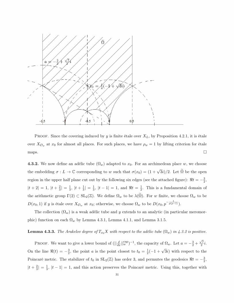
4.3.2. We now define an adélic tube (Ωw) adapted to x0. For an archimedean place w, we choose
the embedding σ : L → C corresponding to w such that σ(x0) = (1 +√3i)/2. Let Ω be the open
region in the upper half plane cut out by the following six edges (see the attached figure): t = −32 ,
|t + 2| = 1, |t + 23 | =
13 , |t +
13 | =
13 , |t − 1| = 1, and t = 1
2 . This is a fundamental domain of
the arithmetic group Γ(2) ⊂ SL2(Z). We define Ωw to be λ(Ω). For w finite, we choose Ωw to be
D(x0, 1) if y is étale over XOwat x0; otherwise, we choose Ωw to be D(x0, p
−1
p(p−1) ).
The collection (Ωw) is a weak adélic tube and y extends to an analytic (in particular meromor-
phic) function on each Ωw by Lemma 4.3.1, Lemma 4.1.1, and Lemma 3.1.5.
Lemma 4.3.3. The Arakelov degree of Tx0X with respect to the adélic tube (Ωw) in 4.3.2 is positive.
Proof. We want to give a lower bound of (|| ddx ||
capw )−1, the capacity of Ωw. Let a = −3
2 +√72 i.
On the line (t) = −32 , the point a is the point closest to t0 = 1
2(−1 +√3i) with respect to the
Poincaré metric. The stabilizer of t0 in SL2(Z) has order 3, and permutes the geodesics t = −32 ,
|t + 23 | =
13 , |t − 1| = 1, and this action preserves the Poincaré metric. Using this, together with
31

the fact that the distance to t0 is invariant under z → −1− z, one sees that the distance from any
point on the boundary of Ω to t0 is at least that from a to t0. Since α : D(0, 1) → H (defined in
the proof of Prop. 4.1.8) preserves the Poincaré metrics, α−1(Ω) contains a disc with respect to the
Poincaré radius equal to the distance from t0 to a.
In D(0, 1), a disc with respect to Poincaré metric is also a disc in the Euclidean sense. Hence
α−1(Ω) contains a disc of Euclidean radius
|α−1(a)| = |(a− t0)/(a− t0)| = 0.45685 · · · .
Since λ maps the fundamental domain Ω isomorphically onto Ωw, by 1.2.3, the local capacity
(|| ddx ||
capw )−1 is at least |(a− t0)/(a− t0)| · |λ(12(−1 +
√3i))|.
By 1.2.3, we have − log(|| ddx ||
capw ) ≥ − log p
p(p−1) when w|p. By Proposition 4.1.8, we have |λ(12(−1+√3i))| = 5.632 · · · . Since
w
− log(|| ddx
||capw ) > log(5.6325 · · ·× 0.45685 · · · )−
p
log p
p(p− 1)> 0.184 · · · ,
we have that deg(Tx0X, || · ||cap) is postive.
Proof of Theorem 3.2.1. Applying Proposition 4.2.1, we have a full set of algebraic solu-
tions y. Choosing the weak adélic tube as in 4.3.2 and applying Corollary 1.2.6 (the assumptions
are verified by 4.3.2 and Lemma 4.3.3), we have that these algebraic solutions are actually rational.
This shows that (M,∇) has a full set of rational solutions over XL. Since formation of ker(∇)
commutes with the finite extension of scalars ⊗KL, this implies that (M,∇) has a full set of rational
solutions over XK .
5. Interpretation using the Faltings height
In this section, we view XZ[ 12 ]
as the moduli space of elliptic curves with level 2 structure. Let
λ0 ∈ X(Q) and E the corresponding elliptic curve. Using the Kodaira–Spencer map, we will relate
the Faltings height of E with our lower bound for the product of radii of uniformizability (see section
4) at archimedean places of the formal solutions in OXK ,λ0 . We will focus mainly on the case when
λ0 ∈ X(Z) and sketch how to generalize to λ0 ∈ X(Q) at the end of this section. In this section,
unlike the previous sections, we will use λ as the coordinate of X.32

5.1. Hermitian line bundles and their Arakelov degrees.
5.1.1. Recall that an Hermitian line bundle (L, || · ||σ) over Spec(OK) is a line bundle L over
Spec(OK), together with an Hermitian metric ||·||σ on L⊗σC for each archimedean place σ : K → C.
Given an Hermitian line bundle (L, || · ||σ), its (normalized) Arakelov degree is defined as:
deg(L) := 1
[K : Q]
log(#(L/sOK))−
σ:K→C
log ||s||σ
,
where s is any section.
For a finite place v over p, the integral structure of L defines a norm || · ||v on LKv. More
precisely, if sv is a generator of LOKvand n is an integer, we define ||pnsv||v = p
−n[Kv :Qp]. We
obtain a norm on Ov by viewing it as the trivial line bundle. We will use || · ||v for the norms on
different line bundle as no confusion would arise. We may rewrite the Arakelov degree using the
p-adic norms:
deg(L) = 1
[K : Q]
−
v
log ||s||v
,
where v runs over all places of K. It is an immediate corollary of the product formula that the right
hand side does not depend on the choice of s.
5.1.2. Let E be an elliptic curve over K, and denote by e : SpecK → E and f : E → SpecK the
identity and structure map respectively. For each σ : K → C, we endow e∗Ω1
E/K = f∗ΩE/K with
the Hermitian norm given by
||α||σ = (1
2π
Eσ(C)|α ∧ α|)
σ
2 ,
where σ is 1 for real embeddings and 2 otherwise.
This can be used to define the Faltings height of E, which we only recall the precise defini-
tion when E has good reduction over OK . Denote by f : E → SpecOK the elliptic curve over
OK with generic fibre E, and again write e for the identity section of E . The norms ||α||σ make
e∗Ω1
E/ Spec(OK) = f∗Ω1E/ Spec(OK) into a Hermitian line bundle, and we define the (stable) Faltings
height by
hF (Eλ) = deg(f∗Ω1E/ Spec(OK)).
33

Notice that hF (Eλ) does not depend on the choice of K. Here we use Deligne’s definition for
convenience [Del85, 1.2]. This differs from the original definition of Faltings (see [Fal86]) by a
constant log(π).
In general, the elliptic curve E will have semi-stable reduction everywhere after some field
extension. We assume this is the case and E has a Neron model f : E → SpecOK which endows
f∗Ω1E/ Spec(OK) a canonical integral structure. With the same Hermitian norm defined as above, we
have a similar definition of Faltings height in the general case. See [Fal86] for details. As in the
good reduction case, this definition does not depend on the choice of K.
5.1.3. We will assume that both λ0 and λ0 − 1 are units at each finite place. Given such a λ0,
consider the elliptic curve Eλ0 over Q(λ0) defined by the equation y2 = x(x− 1)(x−λ0). Then Eλ0
has good reduction at primes not dividing 2, and potentially good reduction everywhere, since its
j-invariant is an algebraic integer. Let K be a number field such that (Eλ0)K has good reduction
everywhere. We denote by Eλ0 the elliptic curve over OK with generic fiber Eλ0 .
5.1.4. To express our computation of radii in terms of Arakelov degrees, we endow the OK-line
bundle Tλ0(XOK), the tangent bundle of XOK
at λ0, with the structure of an Hermitian line bundle
as follows. For each archimedean place σ : K → C, we have the universal covering λ : H → σX,
introduced in 4.1.5. The SL2(R)-invariant metric dt2(t) on the tangent bundle of H induces the
desired metric on the tangent bundle via push-forward. As in the proof of Proposition 4.1.8, our
lower bound on the radius of the formal solution is |2(t0)λ(t0)|σ = || ddλ ||−1
σ , where t0 is a point on
H mapping to λ0. It is easy to see the left hand side does not depend on the choice of t0. Under the
assumptions in 5.1.3, the tangent vector ddλ is an OK-basis vector for the tangent bundle Tλ0(XOK
),
and we havedeg(Tλ0X) =
1
[K : Q](−
σ:K→C
log || ddλ
||σ) ≤1
[K : Q]log(
σ
Rσ),
where the Rσ are the radius of uniformization discussed in section 4.1.
5.2. The Kodaira–Spencer map. Consider the Legendre family of elliptic curves E ⊂ P2Z[ 12 ]
×
XZ[ 12 ]
over XZ[ 12 ]
given by y2 = x(x − 1)(x − λ). We have the Kodaira–Spencer map ([FC90,
Ch. III,9],[Kat72, 1.1]):34

KS : (f∗Ω1E/XZ[ 12 ]
)⊗2 → Ω1XZ[ 12 ]
, α⊗ β → α,∇β,(5.2.1)
where ∇ is the Gauss–Manin connection and ·, · is the pairing induced by the natural polarization.
5.2.1. Following Kedlaya’s notes ([Ked, Sec. 1,3]), we choose dx2y ,
xdx2y to be an integral basis of
H1dR(E/X)|λ0 and compute the Gauss–Manin connection:
∇dx
2y=
1
2(1− λ)
dx
2y⊗ dλ+
1
2λ(λ− 1)
xdx
2y⊗ dλ.
The Kodaira–Spencer map then sends (dx2y )⊗2 to 1
2λ(λ−1)dλ.
This computation shows:
Lemma 5.2.2. Given v a finite place not lying over 2, the Kodaira–Spencer map (5.2.1) preserves
the Ov-generators of (f∗Ω1E/XZ[ 12 ]
)⊗2|λ0 and Ω1XZ[ 12 ]
|λ0 when λ0 and λ0 − 1 are both v-units.
5.2.3. For the archimedean places σ, we consider f∗Ω1σE/SpecC with the metrics ||α||σ defined in
section 5.1, and we endow Ω1XZ |λ0 the Hermitian line bundle structure as the dual of the tangent
bundle.
To see that the Kodaira–Spencer map preserves the Hermitian norms on both sides, one may
argue as follows. Notice that the metrics on (f∗Ω1σE/SpecC)
⊗2 and Ω1XZ are SL2(R)-invariant (see
for example [ZP09, Remark 3 in Sec. 2.3]). Hence they are the same up to a constant and we only
need to compare them at the cusps. To do this, one studies both sides for the Tate curve. See for
example [MB90, 2.2] for a related argument and Lemma 4.1.6 (2) for relation between θ-functions
and Ω1X .
Here we give another argument:
Lemma 5.2.4. The Kodaira–Spencer map preserves the Hermitian metrics:
||(dx2y
)⊗2||σ = || dλ
2λ0(λ0 − 1)||σ.
35
Proof. Let dz be an invariant holomorphic differential of C/(Z⊕ t0Z), where λ(t0) = λ0. By
the theory of the Weierstrass-℘ function, we have a map from the complex torus to the elliptic curve
u2 = 4v3 − g2(t0)v − g3(t0)
such that dz maps to dvu . Here g2 is the weight 4 modular form of level SL2(Z) with 4π4
3 as
the constant term in its Fourier series and g3 is the weight 6 modular form with 8π6
27 as the con-
stant term. Using Lemma 4.1.6 (3), we see that the right hand side has three roots: π2
3 (θ400(t0) +
θ401(t0)),−π2
3 (θ400(t0) + θ410(t0)),
π2
3 (θ410(t0)− θ401(t0)). Hence this curve is isomorphic to y
2 = x(x−
1)(x− λ0) via the map
(5.2.2) x =v − 1
3π2(θ400(t0) + θ
401(t0))
−π2θ401(t0), y =
u
2(−π2θ401(t0))3/2
,
and we havedx
2y= πiθ
201(t0)
dv
u= πiθ
201(t0)dz.
Hence
||(dx2y
)⊗2||σ = |π2θ401(t0) · (
1
2π
E(C)|dz ∧ dz|)|σ = |πθ401(t0)(t0)|v .
On the other hand, using Lemma 4.1.6 (2), we have
|| dλ
2λ0(λ0 − 1)||1/σσ =
2(t0)|λ(t0)|2λ0(λ0 − 1)
=(t0)πθ400(t0)θ410(t0)θ401(t0)λ0(λ0 − 1)
= |πθ401(t0)(t0)|.
Proposition 5.2.5. If λ0 and λ0 − 1 are both units at every finite places, we have deg(Tλ0X) =
−2hF (Eλ0) +log 23 .
Proof. By lemma 5.2.2 and lemma 5.2.4, we have36
−deg(Tλ0X) =deg(Ω1XOK
|λ0)
=1
[K : Q]
−
v
log || dλ
2λ(λ− 1)||v
=1
[K : Q]
−
v|∞
log || dλ
2λ(λ− 1)||v −
v∞
log || dλ
2λ(λ− 1)||v
=1
[K : Q]
−
v|∞
log ||(dx2y
)⊗2||v −
v2∞
log ||(dx2y
)⊗2||v −
v|2
log ||1/2||v
=2hF (Eλ0) +1
[K : Q]
v|2
log ||(dx2y
)⊗2||v − log 2.
(5.2.3)
Now we study ||(dx2y )⊗2||v given v|2. The sum 1[K:Q]
v|2 log ||(dx2y )⊗2||v does not change after
extendingK, hence we may assume that Eλ0 over Ov has the Deuring normal form u2+auw+u = w
3
(see [Sil09] Appendix A Prop. 1.3 and the proof of Prop. 1.4 shows in the good reduction case, a
is a v-integer). An invariant differential generating f∗Ω1Eλ0
/ SpecOK [ 13 ]is dw
2u+aw+1 .
Because both dw2u+aw+1 and dx
2y are invariant differentials, we have
||dx2y
||v = ||∆1/∆2||112v || dw
2u+ aw + 1||,
where ∆1 and ∆2 are the discriminant of the Deuring normal form and that of the Legendre
form respectively. Since E has good reduction, ||∆1||v = 1 (see the proof of loc. cit.). Hence
||dx2y ||v = || dw2u+aw+b ||v · ||1/16||
1/12v = ||2||−1/3
v .
Hence deg(Tλ0X) = −2hF (Eλ0)− 23 log 2 + log 2 = −2hF (Eλ0) +
log 23 .
5.2.6. [Del85, 1.5] mentioned that the point 1+√3i
2 corresponds to the elliptic curve with smallest
height. Hence, our choice 1+√3i
2 gives the largest deg(Tλ0X) among those λ0 such that λ0 and λ0−1
are units at every prime.
5.3. The general case. When λ0 ∈ X(Q), a similar argument as in section 5.2 shows that
1
[K : Q]
−
σ:K→C
log || ddλ
||σ
≤ −2hF (Eλ0) +
log 2
3
+1
[K : Q]
v finite
log+ ||λ0||v + log(|Nmλ0(λ0 − 1)|)(5.3.1)
37

and equality holds if and only if λ0 ∈ X(Z2). As discussed in 5.1.4, the left hand side is the sum of
the logarithms of our estimates of the radii of uniformizability at archimedean places.
We also need to modify the estimate of the radii at finite places in Lemma 3.1.5. A possible
estimate for Rv is p−
1p(p−1) ·min||λ0||v, ||λ0−1||v, 1. One explanation of the factormin||λ0||v, ||λ0−
1||v, 1 is that we cannot rule out the possibility that one has local monodromy at 0, 1,∞ merely
from the information of p-curvature at v.
Compared to the case when λ0 ∈ X(Z), our estimate for the sum of the logarithms of the
archimedean radii increases by at most
1
[K : Q](
v finite
log+ ||λ0||v + log(|Nmλ0(λ0 − 1)|)),
while the estimate for the sum of logarithms of the radii at finite places becomes smaller by
v
maxlog+ ||λ−10 ||v, log+ ||(λ0 − 1)−1||v.
An explicit computation shows that the later is larger than the former. Hence the estimate for the
product of the radii does not become larger than the case when λ0 ∈ X(Z).
6. The affine elliptic curve case and examples
6.1. Statement of the main result of the affine elliptic curve case. Let X ⊂ A2Zbe the
affine curve over Z defined by the equation y2 = x(x− 1)(x+1). The generic fiber XQ is an elliptic
curve (with j-invariant 1728) minus its identity point. Given a vector bundle with connection over
XK , we will define the notion of vanishing p-curvature for all finite places along the same lines as
in section 3.1. The main result of this section is:
Theorem 6.1.1. Let (M,∇) be a vector bundle with connection over XK . Suppose that the p-
curvatures of (M,∇) vanish for all p. Then (M,∇) is étale locally trivial.
Remark 6.1.2. This theorem cannot be deduced from applying Theorem 3.2.1 to the push-forward
of (M,∇) via some finite étale map from an open subvariety of the affine elliptic curve to P1K −
0, 1,∞. Unlike the P1K − 0, 1,∞ case, the conclusion here allows the existence of (M,∇) with
finite nontrivial monodromy. See section 6.3.
Now we explain the meaning of vanishing p-curvature for all p.38

6.1.3. We fix x0 = (0, 0) ∈ X(Z) and denote by (x0)K and (x0)kv the images of x0 in X(K) and
X(kv). Let y : X → A1Zbe the projection to the y-coordinate. It is easy to check that this map
is étale along x0 and hence induces isomorphisms between the tangent spaces Tx0X∼= T0A
1Zand
between the formal schemes XK/(x0)K∼=
A1K/0. In particular, we have an analytic section sv of the
projection y from D(0, 1) ⊂ A1(Kv) to X(Kv) such that sv(0) = x0 for any finite place v by the
lifting criterion for étale maps. By definition, the image sv(D(0, 1)) is the open rigid analytic disc
in X(Kv) which is the preimage of (x0)kv under the reduction map X(Kv) → X(kv).
By choosing a trivialization ofM in some neighborhood of (x0)K , we can view a formal horizontal
section m of (M,∇) around (x0)K as a formal function in OrXK ,(x0)K
∼= OrA1K,0, where r is the rank
of M . We denote f ∈ OrA1K,0
to be the image and the goal of the next subsection is to prove that
the formal power series f is algebraic.
Let U be X − (0, 1), (0,−1). It is a smooth scheme over Z. Our chosen point x0 is a Z-point
of U and sv(D(0, 1)) ⊂ U(Kv). For v a finite place of K with residue characteristic p, we say
that (M,∇) has good reduction at v if (M,∇) extends to a vector bundle with connection on UOv.
Similar to Lemma 3.1.5, we have:
Lemma 6.1.4. Suppose that (M,∇) has good reduction at v. If the p-curvature ψp vanishes2, then
the formal power series f is the germ of some meromorphic function on the disc D(0, p−1
p(p−1) ) ⊂ A1.
Proof. Let (M,∇) be an extension of (M,∇) over XOv. Since y is étale, the derivation ∂
∂y is
regular over some Zariski open neighborhood V of x0 ∈ X⊗Z/pZ. Let V ⊂ X(Kv) be the preimage
of V under reduction map. Since the p-curvature vanishes, we have ∇( ∂∂y )
p(M|V ) ⊂ pM|V . Notice
that sv(D(0, 1)) ⊂ V . Then the proof of Lemma 3.1.5 shows the existence of horizontal sections ofM
on sv(D(0, p−1
p(p−1) )). Via a local trivialization of M and the isomorphism of formal neighborhoods
of x0 and 0, we see that f is meromorphic over D(0, p−1
p(p−1) ).
This lemma motivates the following definition:
Definition 6.1.5. We say that the p-curvatures of (M,∇) vanish for all p if
(1) the p-curvature ψp vanishes for all but finitely many p,
2This means ψp ≡ 0 on XOv ⊗ Z/pZ as in section 3.1.1.
39

(2) all formal horizontal sections around x0, when viewed as formal functions in OrA1K,0, are
the germs of some meromorphic functions on D(0, p−1
p(p−1) ) for all finite places v.
Remark 6.1.6. The second condition does not depend on the choice of local trivialization of M .
Moreover, for each v, this condition remains the same if we replace the projection y by any map
g : WOv→ A
1Ov
such that WOvis a Zariski open neighborhood of (x0)Ov
in XOvand that g is étale.
6.2. Estimate at archimedean places and algebraicity. Let σ : K → C be an archimedean
place. Let φ : D(0, 1) → X(C) be a uniformization map such that φ(0) = x0. We have the following
lemma whose proof is the same as that of Lemma 4.1.1:
Lemma 6.2.1. The σ-adic radius Rσ (see Definition 1.1.2) of the formal functions f in 6.1.3 is at
least |(y φ)(0)|σ.
Let t0 = 1+i2 . A direct manipulation of the definition shows λ(t0) = −1, where λ is defined in
4.1.5. Let F : D(0, 1) → C− (Z+ t0Z) be a uniformization map such that F (0) = 12 .
Lemma 6.2.2 (Eremenko). The derivative |F (0)| = 2−3/2π−3/2Γ(1/4)2 = 0.8346...
Proof. From [Ere11, Sec. 2], we have F(0) = 25/2
B(1/4,1/4) |(λ−1)(i)|3, where B is the Beta
function. By Lemma 4.1.6, the Chowla-Selberg formula ([SC67])
(6.2.1) |η(i)| = 2−1π−3/4Γ(1/4),
and the fact that θ400(i) = 2θ401(i) = 2θ410(i), we have
|(λ−1)(i)| = |πi(θ01(i)θ10(i)θ00(i)
)4| = π|η(i)|4 = Γ(1/4)4
24π2.
We obtain the desired formula by noticing that B(1/4, 1/4) = π−1/2Γ(1/4)2.
Lemma 6.2.3. Let α be the constant 2(−π2θ401(t0))
3/2and ℘ be the Weierstrass-℘ function. We
have y φ = α−1
℘ F , up to some rotation on D(0, 1).
Proof. The map g := (℘,℘) maps C−(Z+ t0Z) to the affine curve u2 = 4v3−g2(t0)v−g3(t0).
Let s be the isomorphism from this affine curve to X(C) given by (5.2.2). Since both s g(1/2) and3The choice of λ there is different. We have λ(i) = 2 here.
40

x0 are the unique point fixed by the four automorphisms of X(C), we have s g(1/2) = x0. Hence
s g F (0) = x0 = φ(0) and then the uniformizations s g F and φ are the same up to some
rotation. Then we have y φ = y s g F = α−1
℘ F by (5.2.2).
Proposition 6.2.4. The σ-adic radius R
[K:Q][Kσ :R]σ ≥ 2−5/2
π−2Γ(1/4)4 = 3.0949 · · · .
Proof. Differentiate both sides of (℘(z))2 = 4(℘(z))3 − g2(t0)℘(z)− g3(t0), we have
℘(1/2) = 6℘(1/2)2 − g2(t0)/2 = −g2(t0)/2,
where the second equality follows from that
℘(1/2) = π2(θ400(t0) + θ
401(t0))/3 = π
2θ401(t0)(λ(t0) + 1)/3 = 0.
By Lemma 4.1.6 and the fact that θ400(t0) = −θ401(t0) = θ
410(t0)/2, we have
|g2(t0)| =4π4
3· 12|θ800(t0) + θ
801(t0) + θ
810(t0)| = 4π4|θ801(t0)|.
Then by Lemma 6.2.3, the absolute value of the derivative of y φ at 0 is
|α−1℘(1/2) · F (0)| = 2−1
π−3|θ01(t0)|−6 · 2π4|θ01(t0)|8 · |F (0)|
= π|θ01(t0)|2 · 2−3/2π−3/2Γ(1/4)2 (by Lemma 6.2.2)
= 2π · 2−2π−3/2Γ(1/4)2 · 2−3/2
π−3/2Γ(1/4)2
= 2−5/2π−2Γ(1/4)4 = 3.0949 · · · ,
(6.2.2)
where the third equality follows from
|θ01(t0)| = 2−1/12|θ00(t0)θ01(t0)θ10(t0)|1/24 = 21/4|η(t0)| = 21/2|η(i)|,
and (6.2.1).
Proof of Theorem 6.1.1. By Proposition 6.2.4, we have
v|∞Rv ≥ 3.0949 · · · . By Defini-
tion 6.1.5, we have log(
v∞Rv) ≥ −
plog p
p(p−1) = −0.761196 · · · . Hence
log(
v
Rv) ≥ log 3.0949 · · ·− 0.761196 · · · = 0.3685 · · · > 0.
We conclude by applying Theorem 1.1.4. 41
6.3. An example with vanishing p-curvature for all p and nontrivial Ggal. Let K be
Q(√−1), X ⊂ A
2Zbe the affine curve defined by y
2 = x(x−1)(x+1), E be the elliptic curve defined
as the compactification of XK , and f : E → E be a degree two self isogeny of E. We will also use
f to denote the restriction of f to XK\P, where P is the non-identity element in the kernel of f .
Let (M,∇) be f∗(OXK\P, d). By definition, Ggal is Z/2Z.
Proposition 6.3.1. The p-curvature of (M,∇) vanishes for all finite places.
Proof. Notice that f extends to a degree two étale cover from E to E over Z[ i2 ]. Then for
finite v 2, the p-curvature of (M,∇) coincides with that of f∗(M,∇) by the fact that p-curvatures
remain the same under étale pull back4. Hence the p-curvature of (M,∇) vanishes as f∗(M,∇) is
trivial.
For v|2, we write (M,∇) out explicitly. Without loss of generality, we may assume that the
isogeny f from the curve y2 = x(x− 1)(x+ 1) to the curve s
2 = t(t− 1)(t+ 1) is given by
t = − i
2(x− 1
x), s =
(1 + i)y
4x(x+
1
x).
Locally around (t, s) = (0, 0), the sections 1, x is an OXKbasis of f∗OXK
and this basis gives rise
to a natural Zariski local extension of (M,∇) over XOp . Direct calculation shows that
∇(1) = 0,∇(x) =2s
(t2 − 1)(3t2 − 1)ds+
2st(1 + 2i)
(t2 − 1)(3t2 − 1)xds.
Therefore, ∇(f1 + f2x) ≡ df1 + xdf2 (mod 2) and the p-curvature of (M,∇) vanishes.
Remark 6.3.2. In the above proof, we show that (M,∇) has all p-curvatures vanishing in the
strict sense: there is an extension of (M,∇) over XOKsuch that its p-curvatures are all vanishing.
However, given the argument for v 2, in order to to apply Theorem 6.1.1, we do not need to
construct an extension of (M,∇) but only need to check that x, locally as a formal power series of
s, converges on D(0, 2−1/2) for v|2. This is not hard to see from the facts: x, as a power series of t,
converges when |t|v < |2|v; and t, as a power series of s, converges when |s|v < |2|1/2v and the image
of |s|v < |2|1/2v is contained in |t|v < |2|v.
4Because p = 2 is unramified in K and (M,∇) has good reduction at p, the notion of p-curvature here is classical.
42

6.4. A variant of the main theorems. We now prove a variant of the main theorems when
X = A1Q− ±1,±i. Similar to Theorem 6.1.1, the conclusion is that (M,∇) has finite monodromy
and we give an example with nontrivial finite monodromy.
In order to define the local convergence conditions for bad primes, we take x0 = 0.
Proposition 6.4.1. Let (M,∇) be a vector bundle with connection over X with p-curvature vanishes
for all finite places. We further assume that the formal horizontal sections around x0 converge over
D(x0, 1) for all finite places v|15. Then (M,∇) is étale locally trivial.
Proof. By Lemma 6.2.2, we have R∞ ≥ 2 · 0.8346 · · · . By the assumptions on finite places, we
have log(
v∞Rv) ≥ −
p =3,5log p
p(p−1) = −0.4976 · · · . We conclude by applying Theorem 1.1.4.
Example 6.4.2. Let s be the algebraic function (1 − x4)1/2. It is the solution of the differential
equation dsdx = −2x3
1−x4 . Consider the connection on OX given by ∇(f) = df + 2x3
1−x4dx. It has p-
curvature vanishing for all p: ∇(f) ≡ df (mod 2) and ∇(f) ≡ df + (p + 1) 2x3
1−x4dx (mod p) with
solution s ≡ (1− x4)(p+1)/2 (mod p) when p = 2. In conclusion, (OX ,∇) satisfies the assumptions
in the above proposition while it has nontrivial monodromy of order two.
Remark 6.4.3. If we replace our assumption by similar conditions on generic radii, the above
example shows that one could have order two local monodromy around ±1,±i. The reason is
[BS82, III eqn. (3)] does not hold in this situation and a modification of their argument would
show that an order two local monodromy is possible.
43

CHAPTER 4
The conjecture of Ogus
Let A be a polarized abelian variety of dimension g defined over a number field K. Let L
be a finite extension of K. For any field F containing K, we denote by HidR(A,F ) the de Rham
cohomology group
HidR(AF /F ) = H
i(AF ,Ω•
AF /F ) = HidR(A/K)⊗K F.
We consider the filtered vector space H1dR(A,L)
m,n and the following semi-linear actions.
Let v be a finite place of L and kv be the residue field. If AL has good reduction at v and
v is unramified in L/Q, we use ϕv to denote the crystalline Frobenius acting on H1dR(A,Lv)m,n
via the canonical isomorphism to the crystalline cohomology (H1cris(Akv/W (kv))⊗Lv)m,n. For any
archimedean place σ corresponding to an embedding σ : L → C, let ϕσ be the map on H1dR(A,C)
m,n
induced by the complex conjugation on (H1B(Aσ(C),Q) ⊗ C)m,n via cBdR. As mentioned in the
introduction, these semi-linear actions define special elements, namely de Rham–Tate cycles (Defi-
nition 7.1.1), in H1dR(A,L)
m,n.1
Theorem 3 and Theorem 4 are proved in section 8 and Theorem 6 is proved in section 9. For
Theorem 3 and Theorem 6, the goal is to prove that GdR and GMT are the same. As a first step,
we prove in section 7 that GdR is reductive and reformulate Bost’s theorem (see Proposition 5) as
that the centralizer of GdR in End(H1dR(A/K)) coincides with that of GMT. To do this, we follow
the construction of motives of absolute Hodge cycles due to Deligne and construct the category
of motives generated by A with morphisms being the de Rham–Tate cycles. We prove that this
category is a semisimple Tannakian category whose fundamental group is GdR ⊂ GSp(H1dR(A/K)).
Then we use the techniques mentioned in the introduction to further show that the centralizer of
G
dR in End(H1dR(A/K)) coincides with that of GMT. The Mumford–Tate conjecture (recalled in
section 8) is an input: we show that this conjecture implies that the rank of G
dR equals to that of
GMT. This allows us to conclude by a lemma of Zarhin. The extra inputs of the proof of Theorem 4
1Here we implicitly take into account the Tate twist as L⊗Q(1) is a direct summand of some H1dR(A,L)m,n
44

are the weakly admissibility of certain filtered ϕ-modules of geometric origin and the Riemann
hypothesis part of the Weil conjectures.
We also discuss a natural variant of de Rham–Tate cycles, the relative de Rham–Tate cycles
(Definition 7.4.1). Here the word ‘relative’ means that to define these cycles, we use relative Frobenii
ϕ[Lv :Qp]v instead of ϕv. In next chapter, we will discuss some results on the conjectural analogue
(Conjecture 7) of Theorem 7.3.7 for relative de Rham–Tate cycles.
Throughout this chapter, we will use End?(A) to denote End?(A)⊗Q, where ? can be K,L or
K. The subscription is omitted if EndK(A) = EndK(A).
7. De Rham–Tate cycles and a result of Bost
In this section, we define de Rham–Tate cycles (section 7.1), de Rham–Tate groups (section 7.2)
and their relative version (section 7.4) and discuss their basic properties. We recall previous results
on absolute Tate cycles in section 7.1 and discuss Proposition 5 in section 7.3.
7.1. De Rham–Tate cycles.
Definition 7.1.1. An element s ∈ (H1dR(A,L))
m,n is called a de Rham–Tate cycle of the abelian
variety A (over L) if there exists a finite set Σ of finite places of L such that for all places v /∈ Σ,
ϕv(s) = s.
Remark 7.1.2.
(1) Similar arguments as in [Ogu82, Cor. 4.8.1, 4.8.3] show that s ∈ (H1dR(A,K))m,n is de
Rham–Tate if and only if its base change in (H1dR(A,L))
m,n is de Rham–Tate and that the
set of de Rham–Tate cycles over L is stable under the natural action of Gal(L/K) (on the
coefficient of de Rham cohomology groups).
(2) Due to [Ogu82, Cor. 4.8.2], although one could define de Rham–Tate cycles over arbitrary
field L containingK, we only need to consider cycles over number fields since any de Rham–
Tate cycle must be defined over Q and hence over some number field.
We have the following important fact, whose proof we sketch for completeness.
Lemma 7.1.3 ([Ogu82, Prop. 4.15]). If s ∈ H1dR(A,L)
m,nis fixed by infinitely many ϕv (for
example, when s is de Rham–Tate), then s lies in Fil0H1dR(A,L)
m,n. Moreover, if such s lies in
Fil1H1dR(A,L)
m,n, then s = 0.
45

Proof. By [Maz73, Thm. 7.6] and the extension of the result to H1dR(A,L)
m,n in the proof by
Ogus2 , we have that for all but finitely many v, the mod p filtration Filj(H1cris(Akv/W (kv)⊗kv)m,n)
is the set ξ mod p | ξ ∈ (H1cris(Akv/W (kv)))
m,n with ϕv(ξ) ∈ pj(H1
cris(Akv/W (kv)))m,n. Then for
the infinitely many v such that ϕv(s) = s, we have that the reduction
s mod p ∈ Fil0((H1cris(Akv/W (kv))⊗ kv)
m,n)
and if s ∈ Fil1H1dR(A,L)
m,n, then s is 0 modulo p. Since the Hodge filtration over L is compatible
with the Hodge filtration over kv, we obtain the desired assertions.
The main conjecture that we study in this chapter is the following:
Conjecture 7.1.4. The set of de Rham–Tate cycles of an abelian variety A defined over K coincides
with the set of Hodge cycles via the isomorphism between Betti and de Rham cohomologies.
Remark 7.1.5.
(1) Our conjecture is weaker than the conjectures of Ogus [Ogu82, Problem 2.4, Hope 4.11.3].
Therefore, Conjecture 7.1.4 was known when A has complex multiplication ([Ogu82, Thm.
4.16]). It was also known when A is an elliptic curve. See [And04b, 7.4.3.1] for an
explanation using Serre–Tate theory.
(2) This conjecture reduces to the case when A is principally polarizable. To see this, note
that after passing to some finite extension of K, the abelian variety A is isogenous to a
principally polarizable one. Moreover this conjecture is insensitive to base change and the
conjectures for two isogenous abelian varieties are equivalent.
Theorem 7.1.6 ([Del82a, Thm. 2.11], [Ogu82, Thm. 4.14], [Bla94]). For any abelian variety,
every Hodge cycle is de Rham–Tate.
Therefore, to prove Conjecture 7.1.4, one only need to show that all of the de Rham–Tate cycles
are Hodge cycles.
2The dual of H1cris(Akv/W (kv)) has a natural W (kv)-structure, although ϕv on the dual does not preserve this integral
structure. In order to apply Mazur’s argument to the dual, Ogus passes to a suitable Tate twist of the dual such thatthe new ϕv acts integrally.
46

7.2. The de Rham–Tate group. We fix an isomorphism of K-vector spaces H1dR(A,K) and
K2g. Then the algebraic group GL2g,K acts on H
1dR(A,K) and hence on H
1dR(A,L)
m,n.
Definition 7.2.1. We define GdR to be the algebraic subgroup of GL2g,K such that for any K-
algebra R, the set of R-valued points GdR(R) is the subgroup of GL2g(R) which fixes all de Rham–
Tate cycles. We call GdR the de Rham–Tate group of the abelian variety A.
Remark 7.2.2. The de Rham–Tate group GdR is naturally defined over K by Remark 7.1.2 (1).
From now on, we use GdR to denote the K-algebraic group.
Lemma 7.2.3. There exists a smallest number field KdR
containing K such that all of the de
Rham–Tate cycles are defined over KdR
. Let sα be a finite set of de Rham–Tate cycles such that
the algebraic group GdR is the stabilizer of all these sα. Then KdR
is the smallest number field such
that all these sα are defined. Furthermore, KdR
is Galois over K.
Proof. Let KdR be the smallest number field over which all sα in the finite set are defined.
We need to show that if t ∈ (H1dR(A, K))m,n is de Rham–Tate, then t is defined over KdR. Let L
be a number field such that t is defined and we may assume L is Galois over KdR. Let W be the
smallest sub vector space of (H1dR(A,K
dR))m,n such that t ∈ W ⊗ L. Let Γ be the Galois group
Gal(L/KdR). Then W ⊗ L is spanned by γt for γ ∈ Γ. By Remark 7.1.2 (1), these γt are de
Rham–Tate, and hence W ⊗ L is spanned by de Rham–Tate cycles. Then by definition, GdR(L)
acts on W ⊗ L trivially and hence so does GdR(KdR) on W . On the other hand, since sα ∪ t
is a finite set, for all but finitely many finite places v of L, we have ϕv(sα) = sα and ϕv(t) = t.
Let p be the residue characteristic of v and let mv be [KdRv : Qp]. The K
dRv -linear action ϕ
mv
v lies
in GdR(KdRv ) since it fixes all sα and hence acts on W ⊗ K
dRv trivially. By definition, ϕv(t) = t
and hence t is stable by ϕmv
v . Therefore, t is defined over KdR by the Chebotarev density theorem
(applying to the coefficients of t expressed in terms of a KdR-base of W ). The last assertion of the
lemma comes from Remark 7.1.2.
7.2.4. Before we reformulate Conjecture 7.1.4 in terms of algebraic groups following Deligne, we
recall the definition and basic properties of the Mumford–Tate group GMT. See [Del82a, Sec. 3]
for details. When we discuss GMT and Hodge cycles, we always fix an embedding σ : K → C. We
denote H1B(Aσ(C),Q) by VB, which has a natural polarized Hodge structure of type ((1, 0), (0, 1)).
47

Let µ : Gm,C → GL(VB,C) be the Hodge cocharacter, through which z ∈ C× acts by multiplication
with z on V1,0B,C and trivially on V
0,1B,C. The Mumford–Tate group GMT of the abelian variety A is the
smallest algebraic subgroup defined over Q of GL(VB) such that its base change to C containing the
image of µ. The Mumford–Tate group is the algebraic subgroup of GL(VB) which fixes all Hodge
cycles.3 Since all Hodge cycles are absolute Hodge cycles in the abelian variety case ([Del82a, Thm.
2.11]), the algebraic group GMT is independent of the choice of σ.
Corollary 7.2.5. Via the de Rham–Betti comparison, we have GdR,C ⊂ GMT,C and the Hodge
cocharacter µ factors through GdR,C.
Proof. It follows from Theorem 7.1.6 and Lemma 7.1.3.
7.2.6. The Mumford–Tate group GMT is reductive ([Del82a, Prop. 3.6]) and the fixed part of GMT
in Vm,nB is the set of Hodge cycles. Conjecture 7.1.4 is equivalent to the following conjecture, which
we will mainly focus on from now on.
Conjecture 7.2.7. Via the de Rham–Betti comparison, we have GdR,C = GMT,C.
Proof of equivalence. Conjecture 7.1.4 implies this conjecture. Conversely, by the discus-
sion in 7.2.6, the isomorphism of these two groups implies that every C-linear combination of de
Rham–Tate cycles maps to a C-linear combination of Hodge cycles via the de Rham–Hodge com-
parison. Then we conclude by Theorem 7.1.6 and Prop. 4.9 in [Ogu82], which shows that all de
Rham–Tate cycles are C-linearly independent.
Remark 7.2.8. This conjecture implies that GdR is connected and reductive. We will show that
GdR is reductive using the same idea of the proof of [Del82a, Prop. 3.6]. However, there seems no
direct way to show that GdR is connected without proving the above conjecture first.
Lemma 7.2.9. The de Rham–Tate group GdR is reductive.
Proof. Fix an embedding σ : K → C. By Corollary 7.2.5, we view GdR,C as a subgroup of
GMT,C ⊂ GL(VB,C). Since all de Rham–Tate cycles are fixed by ϕσ, the subgroup GdR,C is stable
under the action of ϕσ. Therefore, both µ and its complex conjugate µ(= ϕσ µ) factor through
3Here we consider Hodge cycles as elements in Vm,m−2iB
(i) ⊂ Vm
,n
Bfor some choice of m
, n as Tate twists is a
direct summand of the tensor algebra of VB .
48
GdR,C by Corollary 7.2.5 and so does h = µ · µ. Let ψ be the polarization on VB and G1dR,C be the
subgroup of GdR,C acting trivially on the Tate twist. Then ψ is invariant under G1dR,C. Let C be
h(i) ∈ G1dR,C and let φ(x, y) be ψ(x,Cy). Then the positive definite form φ on VB,R is invariant
under adC(G1dR,C)(R)
4. Therefore, G1dR,C has a compact real form adC(G1
dR,C)(R) and is reductive.
Then GdR = G1dR · Z(GdR) is reductive.
7.3. The centralizer of the de Rham–Tate group. The following proposition, whose proof
uses the construction of a Tannakian category of de Rham–Tate cycles, provides a description of
the centralizer of GdR in End(H1dR(A,K)). We will use this proposition to reformulate a result of
Bost. Moreover, at the end of this subsection, we use Corollary 2.2.8 to prove a strengthening of
the result of Bost that will be used to describe the centralizer of G
dR.
Proposition 7.3.1. Let s be an element in (H1dR(A,L))
m,nfor some number field L containing
KdR
. The de Rham–Tate group GdR fixes s if and only if s is a L-linear combination of de Rham–
Tate cycles.
7.3.2. We now construct the category MdRT,L of motives of de Rham–Tate cycles of the abelian
variety A, where L is a field algebraic over K. We follow the idea of the construction of the motive
of absolute Hodge cycles in [Del82b, Sec. 6]. Let A⊗ be the set of varieties generated by A under
finite product and disjoint union, and let HdR(X) be the direct sum of H idR(X,L) for all i.
The objects in the category MdRT,L are of the form
M = (X,n, pr), where X ∈ A⊗, n ∈ Z, pr ∈ End(HdR(X,L)) idempotent de Rham–Tate.
Let Mi = (Xi, ni, pri), i = 1, 2. The set of morphisms Hom(M1,M2) is defined to be
f : HdR(X1)(n1) → HdR(X2)(n2) de Rham–Tate such that f pr1 = pr2 f/ ∼,
where ∼ is defined by modulo f : f pr1 = 0 = pr2 f.
[Ogu82, Prop. 4.9] shows that that MdRT,L is Q-linear with End(I) = Q, where I = (pt, 0, id)
and that Hom(M1,M2) is a finite dimensional Q-vector space. Moreover, by the above construction,
the category MdRT,L is a pseudo-abelian rigid tensor category (see also [And04b, 4.1.3, 4.1.4]).
Since the de Rham–Tate cycles lie in the image of the Betti cohomology with real coefficients4One can check by definition that the C-sub group adC(G1
dR,C) is an R-subgroup of GMT,C.
49

under the Betti–de Rham comparison, pr(HdR(X,C)) has a real Hodge structure. By [Del82b,
Prop. 6.2] and the fact that absolute Hodge cycles are de Rham–Tate cycles, pr(HdR(X,C)) is
polarized. Hence End(M) is semi-simple by [Del82b, Prop. 4.5, Prop. 6.3]. Therefore, we use
[Jan92, Lem. 2] to conclude that MdRT,L is a rigid abelian tensor category. By [Del90, Thm. 1.12],
this is a Tannakian category with a fiber functor ωL : M → pr(HdR(X,L)) over L. Let GLdR be the
Tannakian fundamental group Aut⊗(ωL). Since MdRT,L is semi-simple, GLdR is a reductive algebraic
group over L.
7.3.3. We now describe the relation between de Rham–Tate groups of cycles over different fields.
One can define de Rham–Tate cycles on zero dimensional varieties as in Definition 7.1.1 and define
the motive M0dRT,L as above. This category is the category of Artin motives and we denote by Γ(L)
its Tannakian fundamental group, which is an L-form of the Galois group Gal(L/L). A modification
of the proof of [Del82b, Prop. 6.23] shows that the following sequence is exact:
1 → GLdR → G
LdR → Γ(L) → 1,
where Γ(L) is a quotient of Γ(L). More precisely, Γ(L) is the Tannakian fundamental group of
MdRT,L ∩M0dRT,L, the full subcategory of MdRT,L whose objects are Artin motives.
The category that we will mainly focus on is MdRT,K , which is equivalent to MdRT,KdR by
Lemma 7.2.3, and we will denote them by MdRT.
Proof of Proposition 7.3.1. Let sα be the set of de Rham–Tate cycles. We view GKdR
dR
as a subgroup of GL(H1dR(A,K)) (a priori, GKdR
dR is only defined over KdR, but it descends to K
by Remark 7.1.2(1)). Since MdRT is Tannakian, we have an equivalence of categories
MdRT ⊗ L ∼= RepL(GKdR
dR ).
Hence that s is an L-linear combination of sα is equivalent to that s is fixed by GKdR
dR and it remains
to prove that GKdR
dR = GdR. Since GdR is defined to be the stabilizer of all sα, the above equivalence
of categories shows that GKdR
dR ⊂ GdR. Since GKdR
dR is reductive, then by [Del82a, Prop. 3.1 (b)],
GKdR
dR is the stabilizer of a line in some direct sum of (H1dR(A,L))
m,n. By the definition of GKdR
dR ,
this line must be an L-linear combination of some sα and hence GKdR
dR = GdR because GdR stabilizes
all linear combinations of sα. 50

Remark 7.3.4.
(1) It follows from the proof that GdR is reductive. This argument is essentially the same as
the one we gave before since the key input for both arguments is that de Rham–Tate cycles
are fixed by ϕσ.
(2) There is a variant of Proposition 7.3.1 when L is not assumed to contain KdR. More
precisely, GLdR is the largest subgroup of GL(H1
dR(A,L)) that stabilizes every de Rham–
Tate cycle over L and s ∈ (H1dR(A,L))
m,n is an L-linear combination of de Rham–Tate
cycles over L if and only if s is fixed by the action of GLdR.
The following definition is motivated by [Her12, Def. 3.5].
Definition 7.3.5. An element s of (H1dR(A,L))
m,n is called a β-de Rham–Tate cycle if the A-density
of the set of primes such that φv(s) = s is at most 1− β. More explicitly, it means
β ≤ lim infx→∞
v,pv≤x,ϕv(s)=s
[Lv : Qpv ] log pvpv − 1
[L : Q]
p≤x
log p
p− 1
−1
,
where v (resp. p) runs over finite places of L (resp. Q) and pv is the residue characteristic of v.
Remark 7.3.6.
(1) Absolute Tate cycles and de Rham–Tate cycles are 1-de Rham–Tate cycles by definition.
(2) Let M be a set of rational primes with natural density β and assume that ∀p ∈ M, ∀v|p,
one has ϕv(s) = s. Then s is a β-de Rham–Tate cycle by [Her12, Lem. 3.7].
Theorem 7.3.7. The set of 1-de Rham–Tate cycles in End(H1dR(A,L)) is the image of EndL(A)⊗Q.
In particular, the centralizer of GdR in End(H1dR(A,L)) is EndL(A)⊗ L.
Proof. The second assertion follows from the first one by Proposition 7.3.1 and the above re-
mark. The first statement restricted to absolute Tate cycles is a direct consequence of Theorem 2.0.1
and we refer the reader to [And04b, 7.4.3] for a proof. See also [Bos06, Thm. 6.4]. Notice that
their argument is valid for 1-de Rham–Tate cycles if one uses Corollary 2.2.8 instead.
7.4. Relative de Rham–Tate cycles. Let L be a finite extension over K. Let v be a fi-
nite place of L with residue characteristic p and define mv = [Lv : Qp]. We have an Lv-linear
endomorphism, the relative Frobenius ϕmv
v , of H1dR(A,Lv) and hence of (H1
dR(A,Lv))m,n.51

Definition 7.4.1. An element t ∈ (H1dR(A,L))
m,n is called a relative de Rham–Tate cycle (over L)
of A if there exists a finite set Σ of finite places of L such that for every finite place v /∈ Σ and every
archimedean place σ, one has ϕmv
v (t) = t and ϕmv
v (ϕσ(t)) = ϕσt.
Remark 7.4.2. By definition, any L-linear combination of de Rham–Tate cycles over L is relatively
de Rham–Tate. Moreover, for any γ ∈ Gal(L/K), the cycle γ(t) is relatively de Rham–Tate if (and
only if) t is so.
In analogy with the definition of de Rham–Tate groups, we have:
Definition 7.4.3. We define GL to be the algebraic subgroup of GL2g,L such that any L-algebra
R, its R-points GL(R) is the subgroup of GL2g(R) which fixes all relative de Rham–Tate cycles tα
over L. We call GL the relative de Rham–Tate group of the abelian variety A over L.
Lemma 7.4.4. Similar to the corresponding statements for the de Rham–Tate group, we have:
(1) The relative de Rham–Tate group GLis contained in G
LdR.
(2) Every relative de Rham–Tate cycle lies in Fil0((H1dR(A,L))
m,n) and hence the Hodge cochar-
acter factors through GL.
(3) The group GLis the smallest reductive algebraic subgroup of GL2g,L such that
• the set of its Lv-points contains ϕmv
v for all but finitely many finite places v, and
• it is stable under ϕσ for all archimedean places σ.
(4) Any element in (H1dR(A,L))
m,nis relatively de Rham–Tate if and only if it is fixed by the
action of GL.
Proof. Part (1) follows from Remark 7.4.2. Lemma 7.1.3 implies part (2). To show that GL is
reductive, we notice that ϕσ fixes the set of relative de Rham–Tate cycles and hence the embedding
GLC⊂ GMT,C is induced from an embedding of R-groups. Then, combined with part (2), we see that
µ(i) · µ(i) ∈ GL(C). Now as in the proof of Lemma 7.2.9, the adjoint action of µ(i) · µ(i) defines a
real form of GL which is compact moduo center and hence GL is reductive. The rest of (3) is direct
and it implies (4).
Unlike the de Rham–Tate groups, one can show directly that when L is large enough, the relative
de Rham–Tate group GL is connected. See Corollary 8.1.7.
52
8. Frobenius Tori and the Mumford–Tate conjecture
In this section, we recall the theory of Frobenius tori initiated by Serre (see section 8.1). The
fact that the Frobenius actions on the crystalline and étale cohomology groups have the same
characteristic polynomial ([KM74]) enables us to view the Frobenius tori as subgroups of both
GdR and the -adic monodromy group G. Hence the Frobenius tori serve as bridges between
results for G and those for GdR. We prove a refinement (Proposition 8.1.11) of results of Serre and
Chi on the rank of Frobenius tori. In section 8.2, we recall the Mumford–Tate conjecture and prove
Theorem 3 and Theorem 4. In section 8.3, we recall a result of Noot and use it to show that if G
dR
of A is a torus, then A has complex multiplication.
From now on, we use Σ to denote a finite set of finite places of KdR containing all ramified places
such that for v /∈ Σ, the abelian variety AKdR has good reduction at v and the Frobenius ϕv stabilizes
all of the de Rham–Tate cycles. For any finite extension L of K in question, we still use Σ to denote
the finite set of finite places f−1
g(Σ), where f : SpecL → SpecK and g : SpecKdR → SpecK.
When we discuss the relative de Rham–Tate cycles, we also enlarge Σ so that the relative Frobenius
ϕmv
v stabilizes all relative de Rham–Tate cycles over L.
8.1. Frobenius Tori. The following definition is due to Serre. See also [Chi92, Sec. 3] and
[Pin98, Sec. 3] for details.
Definition 8.1.1. Let Tv be the Zariski closure of the subgroup of GLLv
(hence also of GLdR,Lv
)
generated by the Lv-linear map ϕmv
v ∈ GL(Lv). Since ϕ
mv
v is semisimple, the group Tv is a torus
and is called the Frobenius torus associated to v.
Remark 8.1.2. The torus T v and its rank are independent of the choice of L.
8.1.3. For every prime , we have the -adic Galois representation
ρ : Gal(K/K) → GL(H1ét(AK ,Q))(Q),
and we denote by G(A) the algebraic group over Q which is the Zariski closure of the image
of Gal(K/K) and call G(A) the -adic monodromy group of A. If it is clear which variety is
concerned, we may just use G to denote this group. Serre proved that there exists a smallest finite53
Galois extension Két of K such that for any , the Zariski closure of the image of Gal(Két/Két) is
connected ([Ser13, Sec. 5, p. 15]).
Remark 8.1.4. For v l, we also view Tv as an algebraic subgroup (only well-defined up to
conjugation) of G in the following sense. Since A has good reduction at v, the action of the
decomposition group at v is unramified onH1ét(AK ,Q). Since v is unramified, we have an embedding
Gal(kv/kv) ∼= Gal(Lurv /Lv) → ρ(Gal(K/K)) after choosing an embedding K → Lv. Hence we view
the Frobenius Frobv as an element of G. Due to Katz and Messing [KM74], the characteristic
polynomial of ϕmv
v acting on H1cris(Akv/W (kv)) is the same5 as the characteristic polynomial of
Frobv acting on H1ét(AK ,Q). Hence Tv is isomorphic to the algebraic group generated by semi-
simple element Frobv in G. From now on, when we view Tv as a subgroup of G, we identify Tv
with the group generated by Frobv.
Here are some important properties of Frobenius tori.
Theorem 8.1.5 (Serre, see also [Chi92, Cor. 3.8]). There is a set Mmax of finite places of Két
of natural density one and disjoint from Σ such that for any v ∈ Mmax, the algebraic group Tv is
connected and it is a maximal torus of G.
Proposition 8.1.6 ([Chi92, Prop. 3.6 (b)]). For L large enough (for instance, containing all the
n-torsion points for some n ≥ 3), all but finitely many Tv are connected.
Corollary 8.1.7. For L large enough, the relative de Rham–Tate group GLis connected and G
L =
GL
for L ⊂ L.
Proof. Let (GL) be the connected component of GL. It is reductive and ϕσ-stable for all
archimedean places σ. By Proposition 8.1.6, for all but finitely many v, the group Tv is connected
and hence is contained in (GL)Lv. Therefore, ϕmv
v ∈ Tv(Lv) ⊂ (GL)(Lv) and (GL) = GL by
Lemma 7.4.4(3)(4). Let v be a place of L over v. By definition, Tv is a subgroup of Tv of finite index.
Since Tv is connected, we have φmv
v ∈ Tv = Tv ⊂ GL . We conclude by Lemma 7.4.4(3)(4).
Remark 8.1.8. One reason to introduce relative de Rham–Tate cycles is that GL behaves like G
in the sense that both of them become connected if one replace the base field K by a large enough
L.5To compare the two polynomials, we notice that both of them have Z-coefficients.
54

The following lemma is of its own interest.
Lemma 8.1.9. The number field KdR
is contained in Két.
Proof. For the simplicity of notation, we enlarge KdR to contain K
ét and prove that they
are equal. Let v be a finite place of Két above p such that p splits completely in Két/Q and we
identify Kétv with Qp via v. Let w be a place of KdR above v. Denote by σ the Frobenius in
Gal(KdRw /Qp) = Gal(KdR
w /Kétv ). We consider the algebraic group Tv generated by ϕv ∈ G
Két
dR (Kétv ).
If v ∈ Mmax as in Theorem 8.1.5, then Tv is connected and hence Tv ⊂ GdR,Kétv. This implies
that ϕv ∈ GdR(Kétv ). For any m,n, let W
⊂ (H1dR(A,K
dR))m,n be the KdR-linear span of all de
Rham–Tate cycles in (H1dR(A,K
dR))m,n. By Remark 7.1.2, there exists a K-linear subspace W of
(H1dR(A,K))m,n such that W = W⊗K
dR. Since GdR acts trivially on W and W , the Frobenius ϕv
acts on W ⊗K Kétv trivially and φw acts on W
⊗KdR KdRw as the σ-linearly extension of ϕv. Hence
the elements in W that are stabilized by ϕw are contained in W ⊗K K
étv . That is to say that all de
Rham–Tate cycles are defined over Kétv . As m,n are arbitrary, we have K
dRw = K
étv . This implies
that p splits completely in KdR
/Q and hence KdR = K
ét by the Chebotarev density theorem.
Remark 8.1.10. From Theorem 7.3.7, we see the definition field of a de Rham–Tate cycle induced
from an endomorphism of AK is the same as the definition field of this endomorphism. Hence KdR
contains the definition field of all endomorphisms. Then KdR and K
ét are the same if the definition
field of all endomorphisms is Két. This is the case when one can choose a set of -adic Tate cycles
all induced from endomorphisms of A to cut out G.
Now we discuss some refinements of Theorem 8.1.5 and Proposition 8.1.6. In the rest of this
subsection, the definition field K of the polarized abelian variety A is always assumed to be Galois
over Q. The main result is:
Proposition 8.1.11. Assume that G
(A) is GSp2g,Q. Then there exists a set M of rational primes
with natural density one such that for any p ∈ M and any finite place v of K lying over p, the
algebraic group Tv generated by ϕmv
v (where mv = [Kv : Qp]) is of maximal rank. In particular, Tv
is connected for such v.6
6Our proof is a direct generalization of the proof of Theorem 8.1.5 by Serre. Will Sawin pointed out to me that it ispossible to prove this proposition by applying Chavdarov’s method ([Cha97]) to ResKQ A.
55

The idea of the proof is to apply the Chebotarev density theorem to a suitably chosen Zariski
closed subset of the -adic monodromy group of B, the Weil restriction ResKQA of A. As we are
in characteristic zero, the scheme B is an abelian variety over Q. We have BK =
σ∈Gal(K/Q)Aσ,
where Aσ = A⊗K,σ K. It is a standard fact that B∨ = ResK
QA
∨ and hence the polarization on A
induces a polarization on B over Q. Moreover, the polarization on A induces a polarization on Aσ.
Extend σ to a map σ : K → K. The map σ : A(K) → Aσ(K), P → σ(P ) induces a map on Tate
modules σ : T(A) → T(Aσ). This map is an isomorphism between Z-modules.
Lemma 8.1.12. The map σ : T(A) → T(Aσ) induces an isomorphism between the -adic mon-
odromy groups G(A) and G(Aσ).
Proof. Via σ, the image of Gal(K/K) in End(T(Aσ)) is identified as that of Gal(K/K) in
End(T(A)). Hence G(A) G(Aσ) as T(−)∨ = H1ét((−)K ,Q).
We start with the following special case to illustrate the idea of the proof of Proposition 8.1.11.
Proposition 8.1.13. Assume that G(A) = GSp2g,Qand that A
σis not geometrically isogenous
to Aτfor any distinct σ, τ ∈ Gal(K/Q). Then there exists a set M of rational primes with natural
density 1 such that for any p ∈ M and any v above p, the group Tv is of maximal rank. That is, the
rank of Tv equals to the rank of G(A). In particular, Tv is connected for such v.
Proof. We use the same idea as in the proof of Theorem 8.1.5 by Serre. His idea is to first
construct a proper Zariski closed subvariety Z ⊂ G(A) as follows (see also [Chi92, Thm. 3.7]) and
then to apply the Chebotarev density theorem:
(1) Z is invariant under conjugation by G(A), and
(2) if u ∈ G(A)(Q) \ Z(Q) semisimple, then the algebraic subgroup of G generated by u is
of maximal rank.
Since G(A) is connected, Z(Q) is of measure zero in G(A)(Q) with respect to the usual Haar
measure. We will define a Zariski closed subset W ⊂ G(B) which has similar properties as Z.
Let GK (B) be the Zariski closure of Gal(K/K) in GL(H1
ét(BQ,Q)). Via the isomorphism
H1ét(BQ
,Q) ∼= ⊕H1ét(A
σK,Q) of Gal(K/K)-modules, we view G
K (B) as a subgroup of
G(Aσ).
By the assumption that Aσ’s are not geometrically isogenous to each other and [Lom15, Thm. 4.1,
Rem. 4.3], we have GK (B) ∼= Gm ·
SG(Aσ), where SG ⊂ G is the subgroup of elements with
56

determinant 1. Indeed, LieSG(Aσ) = sp2g,Qof type C and the representations are all standard
representations and then Rem. 4.3 in loc. cit. verified that Lombardo’s theorem is applicable in
our situation. Then By Lemma 8.1.12, we have GK (B) Gm · SG(A)[K:Q]. This is the neutral
connected component of G(B).
The map Gal(Q/Q) → G(B)(Q) → G(B)(Q)/GK (B)(Q) induces a surjection Gal(K/Q)
G(B)(Q)/GK (B)(Q). Given σ ∈ Gal(K/Q), we denote by σG
K (B) the subvariety of G(B)
corresponding to the image of σ in the above map. Let m be the order of σ ∈ Gal(K/Q). We
consider those p unramified in K/Q whose corresponding Frobenii in Gal(K/Q) fall into cσ, the
conjugacy class of σ. We have mv = m for all v above p.
Consider the composite map mτ : σGK (B) → G
K (B) → G(Aτ ) G(A), where the first map
is defined by g → gm and the second map is the natural projection. Let Wσ,τ be the preimage of Z
and Wσ be ∪τ∈Gal(K/Q)Wσ,τ . Since by definition Wσ is a proper Zariski subvariety of the connected
variety σGK (B), the measure of Wσ(Q) is zero.
Claim. If the Frobenius Frobp (well-defined up to conjugacy) is not contained in the conjugacy
invariant set ∪γ∈cσWγ(Q), then for any v|p, the algebraic subgroup Tv ⊂ G(A) is of maximal rank.
Proof. The subvariety ∪γ∈cσWγ is invariant under the conjugation of GK (B) because Z is
invariant under the conjugation of G(A). This subvariety is moreover conjugation invariant under
the action G(B) since τWστ−1 = Wτστ−1 by definition. By second property of Z and the definition
of the map mτ , we see that the image of Frobmp generates a maximal torus in G(Aτ ). For each
v|p, the Frobenius Frobv is the image of Frobmp in G(Aτ ) for some τ and hence Tv is of maximal
rank.
Let W be ∪σWσ. It is invariant under the conjugation of G(B). As each Wσ,τ (Q) is of measure
zero in G(B)(Q), so is W (Q). By the Chebotarev density theorem (see for example [Ser12, Sec.
6.2.1]), we conclude that there exists a set M of rational primes with natural density 1 such that
Frobp /∈ W (Q). Then the proposition follows from the above claim.
Remark 8.1.14. The assumption that G(A) = GSp2g,Qcan be weakened. The proof still works
if one has GK (B) = Gm ·
SG(Aσ). In other words, the proposition holds true whenever [Lom15,
Thm. 4.1, Rem. 4.3] is applicable. For example, when A has odd dimension and is not of type IV
in Albert’s classification.57

The following property of GSp2g is used in an essential way of our proof of Proposition 8.1.11.
It is well-known, but we give a proof for the sake of completeness.
Lemma 8.1.15. If G is an algebraic subgroup of GL(H1ét(AK ,Q)) containing GSp2g,Q
as a normal
subgroup, then G = GSp2g,Q. In particular, G
(A) = GSp2g,Qimplies that G(A) is connected.
Proof. Let g be a Q-point of G. Then ad(g) induces an automorphism of GSp2g,Qby the
assumption that GSp2g,Qis a normal subgroup. As ad(g) preserves determinant, we view ad(g) as
an automorphism of Sp2g,Q. Since Sp2g,Q
is a connected, simply connected linear algebra group
whose Dynkin diagram does not have any nontrivial automorphism, any automorphism of Sp2g,Q
is inner. Hence ad(g) = ad(h) for some Q-point h of Sp2g,Q. Then g and h differ by an element
in the centralizer of Sp2g,Qin GL2g,Q
. Since the centralizer is Gm, we conclude that g is in
GSp2g,Q(Q).
Proof of Proposition 8.1.11. Let B be ResKQA. As in the proof of Proposition 8.1.13, it
suffices to construct a Zariski closed set W ⊂ G(B) such that
(1) W (Q) is of measure zero with respect to the Haar measure on G(B)(Q),
(2) W is invariant under conjugation by G(B), and
(3) if u ∈ G(B)(Q) \W (Q) is semisimple, then the algebraic subgroup of G(B) generated
by u is of maximal rank.
We first show that, to construct such W , it suffices to construct Wσ ⊂ σGK (B) for each
σ ∈ Gal(K/Q) such that
(1) Wσ(Q) is of measure zero with respect to the Haar measure on G(B)(Q),
(2) Wσ is invariant under conjugation by GK (B), and
(3) if u ∈ σGK (B)(Q)\W (Q) is semisimple, then the algebraic subgroup of G(B) generated
by u is of maximal rank.
Indeed, given suchWσ, we defineW to be ∪σWσ. This set satisfies (1) and (3) and is invariant under
conjugation by GK (B). We then define W to be the G(B)-conjugation invariant set generated by
W. Since [G(B) : GK
(B)] is finite, W as a set is a union of finite copies of W and hence satisfies
(1) and (3).
To construct Wσ, let C ⊂ Gal(K/Q) be the subgroup generated by σ. Consider Aττ∈C . We
have a partition C = 1≤i≤rCi with respect to the K-isogeny classes of Aτ . These Ci have the58

same cardinality m/r. For any α ∈ Gal(K/Q), the partition of αC = αCi gives the partition of
Aττ∈αC with respect to the K-isogeny classes.
Consider the map mα : σGK (B) → G
K (B) → G(Aα) G(A) and define Wσ,α to be the
preimage of Z and Wσ to be ∪α∈Gal(K/Q)Wσ,α as in the proof of Proposition 8.1.13. The proof of
the claim there shows that Wσ satisfies (2) and (3).
Now we focus on (1). By the assumption and Lemma 8.1.15, the group G(A) is connected and
hence Z(Q) is of measure zero. Let γ be σr. Consider r : σGK
(B) → γGK (B) defined by g → g
r
and the composite map (m/r)α : γGK (B) → G
K (B) → G(Aα) G(A), where the first map is
defined by g → gm/r and the second map natural projection. Then mα = (m/r)α r. Let Wr be
(m/r)−1α (Z). Then Wσ,α = r
−1(Wr). Since any two of Aττ=α,ασ,··· ,ασr−1 are not geometrically
isogenous, the same argument as in the proof of Proposition 8.1.13 shows that if Wr(Q) is of
measure zero, so is Wσ,α(Q). The rest of the proof is to show that Wr(Q) is of measure zero.
Notice that G
(BK) = Gm ·
σ∈I SG(Aσ) = Gm ·Sp|I|2g, where I is a set of representatives of all
isogeny classes in Aσσ∈Gal(K/Q).
Since the centralizer of GSp2g in GL2g is Gm and G
(B) is a normal subgroup of G(B), the
map (m/r)α is up to a constant the same as the following map:
γGK (B) → IsomQ
(H1ét(A
αγK,Q), H
1ét(A
αK ,Q)) ∼= GL(H1
ét(AαK ,Q)) → GL(H1
ét(AαK ,Q)),
where the first map is the natural projection, the middle isomorphism is given by a chosen isogeny
between Aα and A
αγ , and the last map is g → gm/r.
The fact that γGK (B) normalizes G
(BK) allows us to apply Lemma 8.1.15 to the image of the
above map and see that the above map factors through
GSp(H1ét(A
αK ,Q)) → GSp(H1
ét(AαK ,Q)), g → g
m/r
and hence Wr(Q), being the preimage of a measure zero set under the above map, is of measure
zero.
8.2. The Mumford–Tate conjecture and the proofs of Theorem 3 and Theorem 4.
Conjecture 8.2.1 (Mumford–Tate). For any rational prime , we have G
(A) = GMT(A)⊗Q via
the comparison isomorphism between the étale and the Betti cohomologies.
59

Lemma 8.2.2. If Conjecture 8.2.1 holds for the abelian variety A, then the reductive groups G(A),
GL(A), GdR(A), and GMT(A) have the same rank.
Proof. Conjecture 8.2.1 implies that G and GMT have the same rank. Then by Theorem 8.1.5,
there are infinitely many finite places v such that the Frobenius torus Tv is a maximal torus of GMT.
Since Tv is a subtorus of GL except for finitely many v, we have that GL and hence GdR have the
same rank as GMT by Corollary 7.2.5.
The assertion of the above lemma is equivalent to the Mumford–Tate conjecture by the following
lemma due to Zarhin and the Faltings isogeny theorem (see for example [Vas08, Sec. 1.1]).
Lemma 8.2.3 ([Zar92, Sec. 5, key lemma]). Let V be a vector space over a field of characteristic
zero and H ⊂ G ⊂ GL(V ) be connected reductive groups. Assume that H and G have the same
rank and the same centralizer in End(V ). Then H = G.
Using this lemma, we prove a special case of Conjecture 7.1.4.
Theorem 8.2.4. Assume that the polarized abelian variety A is defined over Q and that G(A)
is connected. Then the centralizer of G
dR in End(H1dR(A,Q)) is End(A) and moreover, Conjec-
ture 8.2.1 implies Conjecture 7.1.4.
Proof. The assumption is equivalent to that Két = Q. Then by Theorem 8.1.5, we see that
Tp is connected for a density one set of rational primes p. Therefore, for such p, the Frobenius
ϕp ∈ Tp(Qp) ⊂ G
dR(Qp) and any s lying in the centralizer of G
dR is fixed by ϕp. In other words,
s is a 1-de Rham–Tate cycle and by Theorem 7.3.7, s ∈ End(A). The second assertion follows
directly from Lemma 8.2.2 and Lemma 8.2.3.
As in [Pin98], we show that if the conjecture does not hold, then GdR is of a very restricted
form when we assume that A is defined over Q and that Két = Q. We need the following definition
to state our result.
Definition 8.2.5 ([Pin98, Def. 4.1]). A strong Mumford–Tate pair (of weight 0, 1) over K
is a pair (G, ρ) of a reductive algebraic group over K and a finite dimensional faithful algebraic
representation of G over K such that there exists a cocharacter µ : Gm,K → GK satisfying:
(1) the weights of ρ µ are in 0, 1, and60

(2) GK is generated by G(K)Gal(K/K)-conjugates of µ.
We refer the reader to [Pin98, Sec. 4, especially Table 4.6, Prop. 4.7] for the list of strong
Mumford–Tate pairs.
Theorem 8.2.6. If the polarized abelian variety A is defined over Q and G(A) is connected, then
there exists a normal subgroup G of G
dR defined over Q such that
(1) (G, ρ) is a strong Mumford–Tate pair over Q, where ρ is the tautological representation
ρ : G ⊂ GdR → GL(H1dR(A,Q)), and
(2) The centralizer of G in End(H1dR(A,Q)) is End(A).
If we further assume that End(A) is commutative, then we can take G to be G
dR.
The following lemma constructs the cocharacter µ.
Lemma 8.2.7. There exists a cocharacter µ : Gm,K → GLK
such that its induced filtration on
H1dR(A, K) is the Hodge filtration. Moreover, different choices of such cocharacters are conjugate
by an element of GLK(K) and for any embedding σ : K → C, we have that µ, as a cocharacter of
GLK⊗σ C, is conjugate to the Hodge cocharacter µσ.
Proof. By lemma 7.4.4 (2) and [Kis10, Lem. 1.1.1], the subgroup P of GLK
preserving the
Hodge filtration is parabolic and the subgroup U of GLK
acting trivially on the graded pieces of
H1dR(A, K) is the unipotent radical of P . Moreover, the action of P on the graded pieces is induced
by a cocharacter of P/U . Then given a Levi subgroup of P , one can construct a cocharacter of GLK
inducing the desired filtration and vice virsa. Therefore, the assertions follow from the existence of
a Levi subgroup over K and the fact that two Levi subgroups are conjugate.
Proof of Theorem 8.2.6. Let µ be some cocharacter constructed in Lemma 8.2.7 and G
be the smallest normal Q-subgroup of G
dR such that G(Q) contains the image of µ. Notice that
different choices of µ are conjugate to each other over Q and hence the definition of G is independent
of the choice of µ.
The weights of ρ µ are 0 or 1 since the non-zero graded pieces of the Hodge filtration on
H1dR(A, K) are at 0 and 1. Since the subgroup of G generated by G
dR(Q) Gal(Q/Q)-conjugates
of µ must be defined over Q and normal in G
dR, this subgroup coincides with G. Since G
dR
61

is connected and reductive and the image of µ is contained in G, the set of G
dR(Q)-conjugates of
µ is the same as the set of G(Q)-conjugates of µ. Hence (G, ρ) is a strong Mumford–Tate pair over Q.
To show (2), by Theorem 7.3.7, it suffices to show that ϕp ∈ G(Qp) for p in a set of natural
density 1. By Theorem 8.1.5, it suffices to show that for any p ∈ Mmax, there exists an integer np7
such that ϕnp
p ∈ G(Qp). Let W ⊂ (H1dR(A,Q))m,n be the largest Q-sub vector space with trivial
G-action. Since G is normal in G
dR, the group G
dR acts on W . Then for all p ∈ Mmax, we have
ϕp ∈ G
dR(Qp) acts on W ⊗ Qp. Since G is reductive, it can be defined to be the subgroup of
GL(H1dR(A,Q)) acting trivially on finitely many such W . Since ϕv ∈ G
dR(Qp) is semi-simple, in
order to show that ϕnp
p ∈ G(Qp), it suffices to prove that the eigenvalues of ϕp acting on W ⊗ Qp
are all roots of unity.
Since W ⊂ (H1dR(A,Q))m,n, the eigenvalues of ϕp are all algebraic numbers. Since Frobp acts
on (H1ét(AQ
,Q))m,n with all eigenvalues being -adic units for = p, the eigenvalues of ϕp are
also -adic units. Now we show that these eigenvalues are p-adic units. Let Hp be the Tannakian
fundamental group of the abelian tensor category generated by sub weakly admissible filtered ϕ-
modules of (H1cris(A/W (Fp)) ⊗ Qp)m,n. For p ∈ Mmax, by [Pin98, Prop. 3.13], Hp is connected.
By Lemma 7.1.3, every de Rham–Tate cycle generates a trivial filtered ϕ-module. Then by the
definition of Hp, Hp(Qp) ⊂ GdR(Qp) and thus Hp(Qp) ⊂ G
dR(Qp). Hence W ⊗ Qp is an Hp-
representation and then by the Tannakian equivalence, the filtered ϕ-module W ⊗ Qp is weakly
admissible. By defintion, µ acts on W ⊗ Qp trivially and hence by Lemma 8.2.7, the filtration on
W ⊗ Qp is trivial. Then the Newton cocharacter is also trivial. In other words, the eigenvalues of
ϕp are p-adic units. By the Weil conjecture, the archimedean norms of the eigenvalues are p(m−n)/2.
Then by the product formula, the weight m−n2 must be zero and all the eigenvalues are roots of unity.
We now prove the last assertion. If G = G
dR, then we have G
dR = GH where H is some
nontrivial normal connected subgroup of G
dR commuting with G and H ∩ G is finite.8 Then H
is contained in the centralizer of G and by (2), we have H ⊂ End(A). By the assumption on
End(A), we see that H is commutative and hence H ⊂ Z(G
dR). We draw a contradiction by
7By standard arguments, one can choose an n independent of p.8To see this, notice that as a connected reductive group, G
dR is the product of central torus and its derived subgroupand the intersection of these two subgroups is finite. Then one uses the decomposition results for tori and semi-simplegroups.
62

showing that Z(G
dR) ⊂ G. By Theorem 8.2.4, we have
Z(G
dR) = G
dR ∩ End(A) ⊂ GMT ∩ End(A) = Z(GMT), and hence Z(G
dR) ⊂ Z(GMT).
On the other hand, for all p ∈ Mmax, the torus Tp ⊂ G. Hence we only need to show that
Z(GMT) ⊂ Tp. Since this statement is equivalent up to conjugation, we only need to show that
Z(GMT ⊗ Q) ⊂ Tp ⊂ GL(H1
ét(AQ,Q)). Since Tp is a maximal torus, we have Tp ⊃ Z
(G). We
then conclude by [Vas08, Thm. 1.2.1] asserting that Z(GMT ⊗Q) = Z(G).
8.3. A result of Noot and its consequence. It is well-known that the Mumford–Tate group
is a torus if and only if A has complex multiplication. In particular, G
dR is a torus when A has
complex multiplication. In this subsection, we will show that the converse is also true.
Lemma 8.3.1. If GLcommutes with µσ for some σ, then A has ordinary reduction at a positive
density of primes of degree one (that is, splitting completely over Q).
Proof. After replacing K by a finite extension, we may assume that µ in lemma 8.2.7 is defined
over K. Let v be a finite place of K with residue characteristic p and assume that p splits completely
inK/Q. ThenKv∼= Qp. Let νv be the Newton (quasi-)cocharacter and fix a maximal torus T ⊂ G
L.
By Lemma 7.4.4 (3), we have that νv factors through GL. As in [Pin98, Sec. 1], we define Sµ (resp.
Sνv) to be the set of GL(Kv) Gal(Kv/Kv)-conjugates of µ (resp. νv) factoring through T (Kv)
in Hom((Gm)Kv, TKv
) ⊗Z R. Since all the GL(Kv)-conjugacy of µ coincide with itself and that µ
is defined over Kv, we have Sµ = µ. By the weak admissibility, we have that Sνv is contained in
the convex polygon generated by Sµ (see [Pin98, Thm. 1.3, Thm. 2.3]). Hence Sνv = Sµ. Then we
conclude that A has ordinary reduction at v by [Pin98, Thm. 1.5] if v /∈ Σ.
Proposition 8.3.2. If GLcommutes with µσ or µv for some σ or v, then A has complex multipli-
cation and hence Conjecture 7.1.4 holds for A.
Corollary 8.3.3. The assumption of Proposition 8.3.2 is satisfied when (GdR) commutes with
either µσ or µv. In particular, A has complex multiplication if and only if (GdR) is a torus.
8.3.4. To prove Proposition 8.3.2, we need following theorem of Noot. Let tα be a finite set of
relative de Rham–Tate cycles over L such that GL is the stabilizer of tα. Let v be a finite place of
L with residue characteristic p such that Lv∼= Qp. We assume that v /∈ Σ and that AL has ordinary
63

good reduction at v. The later assumption holds for infinitely many v under the assumption of
Proposition 8.3.2 by Lemma 8.3.1. Since mv = 1 in our situation, we have ϕv(tα) = tα. Moreover,
tα ∈ Fil0(H1dR(A,L))
m,n by Lemma 7.4.4 (2). Hence tα is a ‘Tate cycle’ in the sense of [Noo96].
In the formal deformation space of Akv , Noot defined the formal locus N where the horizontal
extensions of all tα are still in Fil0(H1dR(A,L))
m,n (see [Noo96, Sec. 2] for details).
On the other hand, for any embedding σ : L → C, the relative de Rham–Tate group GL, viewed
as a subgroup of GMT, is defined over R. Hence GL defines a sub Hermitian symmetric domain
of the one defined by GMT. Let S be the moduli space of polarized abelian varieties of dimension
dimA and let [A] ∈ S be the point corresponding to A. Then the formal scheme associated to the
germ of the image of this sub Hermitian symmetric domain in SC at [A]σ is the formal subscheme
of (S/[A])C defined as the formal locus where all the formal horizontal extensions of tα remain
in Fil0(H1dR(A,L))
m,n. Under the assumption of Proposition 8.3.2, the sub Hermitian symmetric
domain defined by GL is zero dimensional.
Theorem 8.3.5 ([Noo96, Thm. 2.8]). 9The formal locus N is a translate of a formal torus by a
torsion point. Moreover, the dimension of N equals to the dimension of the Hermitian symmetric
space defined by GL.
Proof of Proposition 8.3.2. By Theorem 8.3.5 and the discussion in 8.3.4, ALvis a torsion
point in the formal deformation space. By the Serre–Tate theory, a torsion point corresponds to
an abelian variety with complex multiplication. Hence A has complex multiplication and the last
assertion comes from Remark 7.1.5.
9. Proof of the main theorem
In this section, we prove Theorem 6. In section 9.1, we study the irreducible sub representations
of G
dR in H1dR(A/K) ⊗ K. This part is valid for most abelian varieties without assuming the
Mumford–Tate conjecture. To do this, we focus on the crystalline Frobenii action. The result of
Pink that G with its tautological representation is a weak Mumford–Tate pair over Q provides
information on étale Frobenii and hence information on crystalline Frobenii by a result of Noot
(see9.1.3) relating these two. In section 9.2, we use the results in section 9.1, Theorem 7.3.7 and
9Ananth Shankar pointed out to me that one may use Kisin’s results in [Kis10, Sec. 1.5] and the property of canonicallifting to prove this result.
64

Proposition 8.1.11 to show that under the assumptions of Theorem 6, the centralizer of G
dR in
End(H1dR(A, K)) coincides with that of GdR and then complete the proof of Theorem 6.
9.1. Group theoretical discussions.
9.1.1. Throughout this section, we assume that (GMT(A)Q)der does not have any simple factor
of type SO2k for k ≥ 4. This holds under the assumptions of Theorem 6. The reason for this
assumption is that we will use a result of Noot on the conjugacy class of Frobenius to avoid the
usage of the Mumford–Tate conjecture. It is likely that one can remove this assumption for all the
results in this subsection with some extra work.
Let ρdR : GdR → GL(H1dR(A,K)) be the tautological algebraic representation given in Defini-
tion 7.2.1. We denote by ρK : GdR,K → GL(H1dR(A, K)) the representation on K-points. Assume
that the GdR(K)-representation ρK decomposes as ρK =n
i=1 ρK,i and that each component de-
composes as ρK,i|G
dR,K
=ni
j=1 ρK,i,j , where ρK,i’s (resp. ρK,i,j ’s ) are irreducible representations
of GdR(K) (resp. G
dR(K)). We denote the vector space of ρK,i (resp. ρK,i,j) by Vi (resp. Vi,j).
The following lemma reduces comparing the centralizers of GdR and G
dR to studying the irre-
ducibility of Vi as representations of G
dR,K.
Lemma 9.1.2. If Vi and Vj are not isomorphic as GdR,K-representations, then they are not iso-
morphic as G
dR,K-representations. In particular, if all Vi are irreducible representations of G
dR,K,
then G
dR and GdR have the same centralizer in End(H1dR(A, K)).
9.1.3. Before proving the above lemma, we explain how to use a result of Noot to translate problems
on representations of G
dR into problems on representations of G. We fix an embedding K → Q.
Since the de Rham and étale cohomologies can be viewed as fiber functors of the category of motives
with absolute Hodge cycles, we have an isomorphism of representations of (GMT)Q:
H1dR(A, K)⊗ Q H
1ét(AK ,Q)⊗ Q.
By Theorem 7.3.7, the left hand side, as a representation of (GMT)Q, decomposes into irreducible
ones ⊕Vi ⊗ Q and Vi ⊗ Q∼= Vj ⊗ Q if and only if they are isomorphic as representations of GdR.
Via the above isomorphism, we denote by Véti the image of Vi ⊗ Q. Then by Faltings isogeny
65

theorem, V éti are irreducible representations of (G)Q
and any two of them are isomorphic if and
only if they are isomorphic as representations of (GMT)Q.
Now we study the action of the Frobenius torus T v on both sides. More precisely, we use (T
v )Kv
to denote the base change of the crystalline one acting on the left hand side and use (T v )Q
to denote
the base change of the étale one acting on the right hand side. By [Noo09, Thm. 4.2], after raising
both Frobenius actions to high enough power, ϕmv
v is conjugate to Frobv by an element of GMT10.
Then the weights of the action of T v on Vi and V
éti coincide and that Vi is isomorphic to Vj as
representations of (T v )Kv
is equivalent to that V éti is isomorphic to V
étj as representations of (T
v )Q.
Proof of Lemma 9.1.2. Let v ∈ Mmax as in Theorem 8.1.5. Then Tv is connected and as
a subgroup of G, it is a maximal torus. Since Vi and Vj are not isomorphic as representations
of GdR,K , then by 9.1.3, their counterparts Véti and V
étj are not isomorphic as representations of
(G)Q. Since Tv is a maximal torus, then V
éti and V
étj are not isomorphic as representations of
(Tv)Q. Then by the theorem of Noot (see 9.1.3), Vi and Vj are not isomorphic as representations
of (Tv)Kv. In particular, they are not isomorphic as representations of G
dR.
9.1.4. By construction, we have a fiber functor ω : MdRT → V ecKdR . In other words, ω is a
fiber functor over SpecKdR, viewed as a Q-scheme. The functor Aut⊗(ω) is representable by a
SpecKdR/ SpecQ-groupoid G and G is faithfully flat over SpecKdR ×SpecQ SpecKdR (see [Mil92,
Thm. A.8] or [Del90, Thm. 1.12])11. Let v /∈ Σ (defined in section 8) be a finite place of KdR giving
rise to an embedding KdR → K
dRv . Let Gv be the SpecKdR
v / SpecQp-groupoid obtained by base
changing G to SpecKdRv ×SpecQp
SpecKdRv . Since ϕv(sα) = sα for all de Rham–Tate cycles sα,
the Frobenius semi-linear morphism ϕv lies in Gv(KdRv ). Since G acts on GdR by conjugation, the
action ad(ϕv), the conjugation by ϕv, is an isomorphism between the neutral connected components
10Recall that we use Frobv to denote the relative Frobenius action on the étale cohomology. Noot shows that afterraising to a high enough power, there exists an element g ∈ GMT(K) such that g is conjugate to ϕ
mvv by some element
in GMT(Kv) and that g is conjugate to Frobv by some element in GMT(Q).11Here we use the language of groupoids. One may also view G as a Galois gerb in the sense of Langlands–Rapoportfor the following reason. Since G is a torsor of a smooth algebraic group, it is trivial étale locally and henceG(Q) → (Spec Q×SpecQ Spec Q)(Q) is surjective. We then have the exact sequence (see for example [Mil92, pp. 67])
1 → GdR(Q) → G(Q) → Gal(Q/Q) → 1.
Moreover, GdR, as a group scheme over SpecKdR, is the kernel of G. Let L be the finite extension of KdR such thatall the fiber functors over K
dR are isomorphic over L. Then the extension of Gal(L/L) by GdR(L) induced by theabove sequence splits. Hence G is a Galois gerb in the sense of Langlands–Rapoport.
66

σ∗GdR,KdR
vand GdR,KdR
v, where σ : KdR
v → KdRv is the Frobenius. In terms of KdR
v -points, ad(ϕv)
is a σ-linear automorphism of both GdR(KdRv ) and G
dR(KdRv )12.
Proposition 9.1.5. Assume that AK is simple. Then all ρK,i,j are of the same dimension. More-
over, if we further assume the assumption in 9.1.1 and that a maximal subfield of EndK(A) is
Galois over Q or that EndK(A) is a field, then there exists a choice of decomposition
Vi such that
ϕv(Vi,j) = Vσ(i),τv,i(j), where σ is a permutation of 1, · · · , n and for each i, τv,i is a permutation
of 1, · · · , ni.
Proof. We fix a finite extension L of K such that all the Vi,j are defined over L. Let v /∈ Σ be
a place of L. As discussed in 9.1.4, ad(ϕv) preserves the set G
dR(Lv). Therefore, for any nonzero
vector vi,j ∈ Vi,j , as Qp-linear spaces,
ϕv(Vi,j) = ϕv(SpanLv(G
dR(Lv)(vi,j))) = SpanLv(ϕv(G
dR(Lv)(vi,j)))
= SpanLv(ad(ϕv)(G
dR(Lv)(ϕv(vi,j)))) = SpanLv(G
dR(Lv)(ϕv(vi,j))).
In other words, as an Lv-vector space, ϕv(Vi,j) is the same as the space of the irreducible
G
dR(Lv)-sub representation generated by ϕv(vi,j). Similarly for Vi, we have that the vector space
ϕv(Vi) is the same as the vector space of an irreducible GdR(Lv)-sub representation. In partic-
ular, ϕv(Vi,j) is contained in
dimVk,l=dimVi,jVk,l. Let V
be
dimVk,l=dimVi,jVk,l and V
be
dimVk,l =dimVi,jVk,l. Then ϕv(V ) = V
and ϕv(V ) = V. Let pr
be the projection to V.
Then ϕv(pr) = pr for all v /∈ Σ. By Theorem 7.3.7, pr is an algebraic endomorphism of A. Since
A is simple, pr cannot be a nontrivial idempotent and then V = 0, which is the first assertion.
The second assertion is an immediate consequence of the following two lemmas. Indeed, by
Lemma 9.1.7, we see that the only sub representations in Vs of G
dR are Vs,j ’s. Since ϕv(Vi,j) is a
sub representation of ϕv(Vi) = Vs for some s by Lemma 9.1.6, then ϕv(Vi,j) is Vs,t for some t.
Lemma 9.1.6. Under the assumptions in Proposition 9.1.5, there exists a decomposition H1dR(A,L) =
Vi where Vi are irreducible representations of GdR such that for any i, as vector spaces, ϕv(Vi) =
Vj for some j.
12Although ad(ϕv) defines a σ-linear automorphism of GdR(KdRv ), this fact itself does not imply that GdR,KdR
vhas
a Qp-structure since a priori we do not have the cocycle condition. However, GdR,KdR
vhas a Qp-structure because
MdRT ⊗KdRv has a fiber functor over Qp. The Qp-fiber functor can be chosen to be the étale realization because all
the de Rham–Tate cycles lie in (H1ét(AKv
,Qp))m,n via the p-adic de Rham-étale comparison.
67
Proof. When End(A) is a field, the decomposition is unique and any two different Vj ’s are
not isomorphic. In other words, Vj ’s are the only irreducible sub representations of GdR. Since the
vector space ϕv(Vi) is the vector space of an irreducible sub representation, it must be Vj for some
j.
Now we assume that the maximal subfield of EndK(A) is Galois over Q. Let sα be a Q-basis
of de Rham–Tate cycles in End(H1dR(A,K
dR)). By Theorem 7.3.7, these sα are algebraic cycles
and we use sBα to denote their images in End(H1B(AC,Q)). Since A is simple, EndK(A) is a division
algebra D of index d over some field F and sBα is a basis of D as a Q-vector space. Let E ⊂ D be
a field of degree d over F . Then E is a maximal subfield of D and D ⊗F E ∼= Md(E). Therefore,
D ⊗Q E ∼= D ⊗Q F ⊗F E ∼= D ⊗F E ⊗Q F ∼= Md(E)[F :Q].
Let ei ∈ Md(E) be the projection to the i-th coordinate. Let eji ∈ D ⊗Q E be the element whose
image in Md(E)[F :Q] is (0, .., 0, ei, 0, ..., 0), where ei is on the j-th component. Since
eji is the
identity element in D, there must exist at least one eji such that
τ∈Gal(E/Q) σ(e
ji ) is nonzero,
where the Galois group acts on the coordinates when the basis of the E-vector space D ⊗Q E is
chosen to be a basis of D as a Q-vector space.
We write eji =
kαs
Bα , where kα ∈ E, and let prτ =
τ(kα)sα ∈ End(H1
dR(A, K)), for all
τ ∈ Gal(E/Q). Since eji is an idempotent, so is prτ . Let Vτ be the image of prτ . We may assume
that L contains E and still use σ to denote the image of the Frobenius via the map Gal(Lv/Qp) ⊂
Gal(L/Q) → Gal(E/Q). Then by definition, as vector spaces, ϕv(Vτ ) = Vστ .
Now it remains to prove that
Vτ is a direct sum and
Vτ = H1dR(A, K) as representations
of GdR. First, since prτ lies in the centralizer of GdR, every Vτ is a subrepresentation. Second, since
the number of irreducible representations in a decomposition of H1dR(A, K) equals [E : Q], it suffices
to prove that
Vτ = H1dR(A, K). Since the image of
prτ is contained in
Vτ , it suffices to
prove that
prτ is invertible. By construction,
prτ lies in D (via comparison) and it is nonzero
by the choice of eji . Therefore,
prτ is invertible since D is a division algebra.
Lemma 9.1.7. Under the assumption in 9.1.1, the G
dR-representations Vi,j and Vi,j are not iso-
morphic if j = j.
68
Proof. Let Tw be a Frobenius torus of maximal rank for some finite place w /∈ Σ. We only
need to show that the weights of Tw acting on Vi are all different. By 9.1.3, we may consider Tw
as a maximal torus of G(A) acting on irreducible sub representations of (G)Qin H
1ét(AK ,Q) ⊗
Q. [Pin98, Thm. 5.10] shows that (G(A), ρ) is a weak Mumford–Tate pair over Q. To show
the weights on Vi are different, it suffices to show that the weights of the maximal torus of each
geometrical irreducible component of (G(A), ρ) are different. Furthermore, it reduces to the case
of an almost simple component of each irreducible component. They are still weak Mumford–Tate
pairs by [Pin98, 4.1]. One checks the list of simple weak Mumford–Tate pairs in [Pin98, Table 4.2]
to see that all the weights are different.
9.2. Proof of Theorem 6.
9.2.1. Since the Mumford–Tate conjecture holds for all the abelian varieties considered in Theo-
rem 613, we focus on comparing the centralizers of GdR and G
dR in End(H1dR(A, K)). Once we
prove that the centralizers of both groups are the same, we conclude the proof of Theorem 6 by
Theorem 7.3.7, Lemma 8.2.2, and Lemma 8.2.3 as in the proof of Theorem 8.2.4. We separate the
cases using Albert’s classification.
Type I. Let F be the totally real field EndK(A) of degree e over Q. [BGK06] shows that
Conjecture 8.2.1 holds when g/e is odd.
Proposition 9.2.2. If e = g, then Conjecture 7.1.4 holds for A.
Proof. The Q-vector space H1B(A,Q) has the structure of a two-dimensional F -vector space.
Therefore, as a (GMT)Q-representation, H1B(A,Q) decomposes into g non-isomorphic irreducible sub
representations of dimension two. By 9.1.3, the GdR,K-representation H1dR(A, K) decomposes into
g non-isomorphic irreducible sub representations V1, . . . , Vg. By Lemma 9.1.2 and 9.2.1, we only
need to show that all Vi are irreducible G
dR-representations. By Proposition 9.1.5, if any G
dR-
representation Vi is reducible, then all V1, . . . , Vg are reducible. In such situation, all Vi decompose
into one-dimensional representations and hence G
dR is a torus. Then by Corollary 8.3.3, A has
complex multiplication, which contradicts our assumption. 13The Mumford–Tate conjecture for Ai is well-studied and we will cite the results we need for each case later inthis subsection. See for example [CF16] for a survey of type I and II cases. The reduction of the conjecture for theproduct of Ai to the simple case is essentially contained in [Lom15, Sec. 4] and we record a proof at the end of thissubsection.
69

Remark 9.2.3. The above proof is still valid if all (equivalently, any) Vi are of prime dimension.
Now we focus on the case when EndK(A) = Z. We refer the reader to [Pin98] for the study of
Conjecture 8.2.1 in this case. In particular, Conjecture 8.2.1 holds when 2g is not of the form a2b+1
or4b+22b+1
, where a, b ∈ N\0 and in this situation, G(A) = GSp2g,Q
.
Proposition 9.2.4. Assume that G(A) = GSp2g,Q. If A is defined over a number field K which
is Galois over Q of degree d prime to g!, then Conjecture 7.1.4 holds for A.
Proof. Conjecture 8.2.1 holds when G(A) = GSp2g. It suffices to show that H1dR(A, K) is an
irreducible G
dR,K-representation. If not, then by Proposition 9.1.5, H1
dR(A, K) would decompose
into r sub representations of dimension 2g/r. By Corollary 8.3.3, r cannot be 2g and hence r ≤ g.
Let prj be the projection to the jth irreducible component. By Proposition 9.1.5, we have ϕv(prj) =
prk for some k and the action of ϕv on all prj gives rise to an element sv in Sr, the permutation
group on r elements. On the other hand, by Proposition 8.1.11, there exists a set M of rational
primes of natural density 1 such that for any p ∈ M and any v|p, we have that ϕmv
v ∈ G
dR. Hence
smv
v is the identity in Sr for such v. By the assumption, mv is prime to r! and hence sv is trivial in
Sr. In other words, prj is a 1-de Rham–Tate cycle. Then by Theorem 7.3.7, prj is algebraic, which
contradicts with that A is simple.
Type II and III. In this case, EndK(A) is a quaternion algebra D over a totally real field F of
degree e over Q. [BGK06] and [BGK10] show that if g/(2e) is odd, then Conjecture 8.2.1 holds.
Proposition 9.2.5. If g = 2e, then Conjecture 7.1.4 holds for A.
Proof. The GdR,K-representation H1dR(A, K) decomposes into V1 ⊕ · · · ⊕ Vg where Vi is two
dimensional and Vi is not isomorphic to Vj unless i, j = 2k − 1, 2k. Then we conclude by
Remark 9.2.3.
Type IV. In this case, EndK(A) is a division algebra D over a CM field F . Let [D : F ] = d2
and [F : Q] = e. Then ed2|2g.
Proposition 9.2.6. If 2ged is a prime, then the centralizer of G
dR in EndK(H1dR(A, K)) is the same
as that of GdR.
70

Proof. We view H1B(A,Q) as an F -vector space and hence view GMT as a subgroup of GL2g/e.
Since the centralizer of GMT is D, then H1B(A,Q)⊗F F decomposes into d representations of dimen-
sion 2g/(ed). Hence H1B(A, Q) as a GMT-representation would decompose into de representations
of dimension 2g/(de). Then we conclude by Remark 9.2.3.
Corollary 9.2.7. If g is a prime, Conjecture 7.1.4 holds for A of type IV.
Proof. Notice that when g is a prime, then d must be 1 and e must be 2 or 2g. The second
case is when A has complex multiplication and Conjecture 7.1.4 is known. In the first case, 2ged (= g)
is a prime. Then Conjecture 7.1.4 is a consequence of Proposition 9.2.6 and the Mumford–Tate
conjecture ([Chi91, Thm. 3.1]) by Lemma 8.2.3.
Corollary 9.2.8. If the dimension of A is a prime and EndK(A) is not Z, then Conjecture 7.1.4
holds.
Proof. If g = 2, then A has CM or is of type I with e = g or is type II with g = 2e. If g
is an odd prime, then A is of type I with e = g or of type IV. We conclude by Proposition 9.2.2,
Proposition 9.2.5, and Corollary 9.2.7.
Proof of Theorem 6. Conjecture 7.1.4 is equivalent for isogenous abelian varieties and then
we may assume that A =
Ani
i . By 9.2.1 and the following lemma, it suffices to show that
G
dR(A) and GdR(A) have the same centralizer. By Lemma 9.1.2, the agreement of the centralizers
of G
dR(A) and GdR(A) is equivalent to that all irreducible sub representations in H1dR(A, K) of
GdR(A)K are irreducible representations of G
dR(A)K . Let V be an irreducible representation of
GdR(A)K . Since the projection A → Ai is a de Rham–Tate cycle, then there exists Ai such that
V ⊂ H1dR(Ai, K) and V is an irreducible representation of GdR(Ai)K . Then by Remark 7.1.5 (1),
Corollary 9.2.8, and Proposition 9.2.4, the de Rham–Tate group GdR(Ai) is connected. Then the
surjective map GdR(A) → GdR(Ai) remains surjective when restricted to G
dR(A). This implies that
V is an irreducible representation of G
dR(A)K .
Lemma 9.2.9. Let A be as in Theorem 6. Then the Mumford–Tate conjecture holds for A.
Proof. The idea of the proof is the same as that of [Lom15, Thm. 4.7]. For the simplicity
of statements, we assume that each simple factor of all abelian varieties mentioned in the proof71
falls into one of the three cases in the assumption of the theorem. Notice that an absolutely simple
abelian variety Ai of type IV either have complex multiplication or is of case (2) with EndK(Ai)
being an imaginary quadratic field. Therefore, by assumption, A is either B×C1 or B×Ck2 where B
has no simple factor of type IV, C1 has complex multiplication, and C2 is absolutely simple of case
(2) type IV. By [Lom15, Prop. 2.8] and corresponding statement for the Mumford–Tate group, it
suffices to show that the Mumford–Tate conjecture holds for B × Ci.
We first prove that the Mumford–Tate conjecture holds for B. Let H(B) be the neutral
connected component of the subgroup of G(B) with determinant 1. Since B does not have simple
factor of type IV, the group H(B) is semisimple. By assumption, the Lie algebra of each simple
component of H(B)Q
is of type C and then by [Lom15, Thm. 4.1, Rem. 4.3], the group H(B) =
H(Bi), where Bi is a set of all non-isogeny simple factors of B. Since the Mumford–Tate
conjecture holds for Bi, then the conjecture holds for B by [Lom15, Lem. 3.6].
On the other hand, H(C1) is a torus and the Lie algebras of simple factors H(C2)Qare of
type Ap−1 for p ≥ 3 prime14. Since Lie algebra of type Ap−1 is not isomorphic to that of type C,
we apply [Lom15, Prop. 3.9, Lem. 3.6] to conclude that the Mumford–Tate conjecture holds for
B × Ci.
14Notice that there does not exist a non-CM abelian surface of type IV.
72

CHAPTER 5
A relative version of Bost’s theorem
In section 10, we prove Theorem 8. Roughly speaking, the main idea is to prove that the relative
de Rham–Tate group GL (see section 7.4) coincides with the de Rham–Tate group GdR when L is
large enough. In section 11, we prove a result (Corollary 11.1.2) towards Conjecture 7. Given a
relative de Rham–Tate cycle s in End(H1dR(A,L)), Conjecture 7 predicts that if s is a β-de Rham–
Tate cycles (Definition 7.3.5) in End(H1dR(A,L)) with β >
12 , then s is algebraic. We prove that
even without the assumption of being a relative de Rham–Tate cycle, as long as β >34 , a β-de
Rham–Tate cycle in End(H1dR(A,L)) is algebraic.
10. The known cases
We observe that for L/L finite extension, if L ⊃ K
dR, then Conjecture 7 for L implies the
conjecture for L. Hence throughout this section, we may assume that L is large enough so that all
but finitely many Tv are connected. Proposition 8.1.6 shows that such L exists and Corollary 8.1.7
shows that GL is connected. For any finite place v of L, we write mv = [Lv : Qp].
10.1. Relative de Rham–Tate cycles revisited. The cycles considered in Conjecture 7
motivate the following definition. It is weaker than the notion of relative de Rham–Tate cycles as
we put no restrictions on archimedean places.
Definition 10.1.1. An element t ∈ (H1dR(A,L))
m,n is called a weakly relative de Rham–Tate cycle
(over L) of A if there exists a finite set Σ of finite places of L such that for every finite place v /∈ Σ,
one has ϕmv
v (t) = t. When there is no risk of confusion, we simply call t a weakly relative cycle.
Conjecture 7 asserts that any weakly relative cycles in End(H1dR(A,L)) is an L-linear com-
bination of algebraic cycles. This conjecture can be verified when Két = Q as in the proof of
Theorem 8.2.4.
Theorem 10.1.2. If the polarized abelian variety A is defined over Q and G(A) is connected, then
Conjecture 7 holds.
73

Proof. We may assume that L/Q is Galois. Let t ∈ End(H1dR(A,L)) be a weakly relative
cycle. By definition, for any γ ∈ Gal(L/Q), the cycle γ(t) is also weakly relative. Consider the
vector space VL = SpanL(γ(t)γ∈Gal(L/Q)). There is a vector space V ⊂ End(H1dR(A,Q)) such
that VL = V ⊗ L. Let sα be a Q-basis of V . By definition, for v /∈ Σ, the relative Frobenius
ϕmv
v fixes VL and hence sα. In other words, for all but finitely primes p, the Frobenius torus Tp
fixes sα. By Theorem 8.1.5, for p ∈ Mmax of natural density one, ϕp ∈ Tp = Tp fixes sα. Then by
Theorem 7.3.7, sα is algebraic and hence t is a linear combination of algebraic cycles.
Remark 10.1.3. If one replaces Theorem 8.1.5 by our refinements of Serre’s theorem in section 8.1,
the proof of the above theorem shows that, under the assumption of Proposition 8.1.11 or Propo-
sition 8.1.13, one can reduce the verification of Conjecture 7 for any L to the following statement:
if t ∈ End(H1dR(A,K)) is fixed by ϕ
mv
v for all v with residue characteristic in a subset of rational
primes of natural density one, then t is a linear combination of algebraic cycles. Here we assume
that K/Q is Galois and that G(A) is connected.
For relative de Rham–Tate cycles, we have:
Proposition 10.1.4. If the polarized abelian variety A is defined over Q and G(A) ∼= GMT(A)⊗Q,
then all relative de Rham–Tate cycles are linear combinations of Hodge cycles.
Proof. As in the proof of Theorem 8.2.4, one can show that ϕp ∈ GL(Qp) for a density one
set of rational primes and hence GL has the same centralizer as GMT and then the rest of the proof
is the same.
Proposition 10.1.5. If the polarized abelian variety A is defined over Q and G(A) is connected,
then Theorem 8.2.6 still holds with G
dR replaced by GL.
Proof. The key steps of the proof of Theorem 8.2.6 are as follows. By Lemma 8.2.7, we
construct the smallest normal Q-subgroup G of G
dR containing µ. Then one uses weak admissibility
and the Riemann Hypothesis part of the Weil conjecture to show that some power of ϕp lies in G
for all p. Finally by Theorem 8.1.5 and Theorem 7.3.7, G has the same centralizer as GMT and
one uses a result of Vasiu to see that G is G
dR when the endomorphism ring of A is commutative.
Every step is still valid with G
dR replaced by GL.
74

10.2. Special cases of Conjecture 7. In this subsection, we prove that for A as in Theorem 8,
all the weakly relative cycles are linear combinations of Hodge cycles. This assertion implies the
theorem.
Theorem 10.2.1. Let A be an abelian variety and L ⊃ KdR = K
ét. All weakly relative cycles over
L of A are L-linear combinations of Hodge cycles if one of the following holds
(1) A has complex multiplication;
(2) A is either an elliptic curve or abelian surface with quaternion multiplication.
Proof. For (1), we fix a finite set Σ of finite places of L such that for all v /∈ Σ, the Frobenius
ϕmv
v fixes all weakly relative cycles over L. By Theorem 8.1.5 and the fact that G
= GMT is a torus,
there exists a finite place v /∈ Σ with mv = 1 such that Tv = GMT ⊗ Lv. By definition, a weakly
relative cycle is fixed by ϕv and hence GMT. In other words, this cycle is a linear combination of
Hodge cycles.
For (2), we may assume that A does not have complex multiplication. Let G be the subgroup
of GL(H1dR(A,L)) that fixes all weakly relative cycles and we shall prove that G = GMT ⊗ L.
Since G
= GMT ⊗ Q, then by Theorem 8.1.5, G contains a maximal torus of GMT ⊗ L. Since
GMT ⊗ Q = GL2, if G = GMT ⊗ L, then G is either a maximal torus or contains a Borel subgroup.
If G contains a Borel subgroup, then the set of cycles fixed by G coincides the set of cycles fixed by
GMT⊗L. In other words, the set of weakly relative cycles agrees with the set of L-linear combination
of Hodge cycles and G = GMT⊗L. If G is a torus, then GL ⊂ G is a torus. We draw a contradiction
by Corollary 8.3.3.
11. A strengthening of Theorem 7.3.7 and its application
We use A∨, E(A) to denote the dual abelian variety and the universal vector extension of A. For
simplicity, when there is no risk of confusion, we use β-cycles to indicate β-de Rham–Tate cycles.
The main result of this section is Corollary 11.1.2 and the idea is to apply Theorem 2.2.5. At the
end of this section, we use Corollary 11.1.2 to study cycles of abelian surfaces.
11.1. A strengthening of Theorem 7.3.7. If s ∈ End(H1dR(A, K)) is a β-cycles for some
positive β, then ϕv(s) = s for infinitely many v and thus s ∈ Fil0(End(H1dR(A, K))) by Lemma 7.1.3.
75

In other words, s(Fil1(H1dR(A, K))) is contained in Fil1(H1
dR(A, K)). Since
H1dR(A, K)/Fil1(H1
dR(A, K)) ∼= LieA∨
K ,
the cycle s then induces an endomorphism s of LieA∨
K.
Theorem 11.1.1. Assume that AK is simple. If s ∈ End(H1dR(A, K)) is a β-de Rham–Tate cycle
for some β >34 , then s is the image of some element in EndK(A∨).
Before proving the theorem, we use it to prove a strengthening of Theorem 7.3.7.
Corollary 11.1.2. Assume that AK is simple. If s ∈ End(H1dR(A, K)) is a β-de Rham–Tate cycle
for some β >34 , then s is algebraic.
Proof. By Theorem 11.1.1, it suffices to show that if s is fixed by infinitely many ϕv and s is
algebraic, then s is algebraic. Since the restriction to EndL(A) of the map
Fil0 End(H1dR(A,L)) → End(LieA∨
L), s → s
is the natural identification EndL(A) ∼= EndL(A∨), we obtain an algebraic cycle t ∈ EndK(A) such
that t = s. Then for infinitely many v, we have ϕv(s− t) = s− t and s− t ∈ Fil1(End(H1dR(A, K)).
By Lemma 7.1.3, s− t = 0 and hence s is algebraic.
Remark 11.1.3. The only place where we use the assumption of AK being simple is to obtain the
first assertion of Lemma 11.1.5. This assertion shows that if s is not algebraic, then the Zariski
closure of the g-dimensional formal subvariety that we will construct using s is of dimension 2g. In
general, the Zariski closure of a non-algebraic g-dimensional formal subvariety is of dimension at
least g + 1 and then the same argument as below shows that any β-cycle with β > 1 − 12(g+1) is
algebraic.
11.1.4. The proof of this theorem will occupy the rest of this subsection. Since the definition of
β-cycle is independent of the choice of a definition field and the property of being a β-cycle is
preserved under isogeny, we may assume that A is principally polarized and that s is defined over
K. Let X be A∨ × A
∨ and e be its identity. The main idea is to apply Theorem 2.2.5 to the76
following formal subvariety V ⊂ X/e. Consider the sub Lie algebra
H = (a, s(a)) | a ∈ Lie(A∨) ⊂ Lie(X).
This sub Lie algebra induces an involutive subbundle H of the tangent bundle of X via translation.
The formal subvariety V is defined to be the formal leaf passing through e. Recall that in 2.2.4 a
finite place v of K is called bad if H⊗ kv is not stable under p-th power map of derivatives.
Lemma 11.1.5. If s is not algebraic, then the formal subvariety V is Zariski dense in X. The
A-density of bad primes is at most 1− β.
Proof. The Zariski closure G of V must be an algebraic subgroup of X. The simplicity of A
implies that the only algebraic subgroup of X with dimension larger than g must be X. Hence if s
is not algebraic, we have dimG > g and hence G = X.
By [Mum08, p. 138], given v /∈ Σ, the p-th power map on LieE(A∨) ⊗ kv = H1dR(A, kv) is
the same as ϕv ⊗ kv. Therefore, for those v such that ϕv(s) = s, we have that the Lie subalgebra
(a, s(a)) | a ∈ (LieE(A∨))⊗ kv of Lie(E(A∨)×E(A∨))⊗ kv is closed under the p-th power map.
Then H = (a, s(a)) | a ∈ Lie(A∨)⊗kv and H⊗kv are closed under the p-th power map. Therefore,
the density of bad primes is at most one minus the density of primes satisfying ϕv(s) = s.
11.1.6. Let σ : K → C be an archimedean place of K. We define γσ to be the composition
γσ : Cg (id,s)−−−→ Cg × C
g (exp,exp)−−−−−−→ Xσ,
where exp the uniformization of Cg = LieA∨σ → A
∨σ . We choose an ample Hermitian line bundle L
on A∨ such that the pull back of its first Chern form via exp is iC0
gk=1 dzk ∧ dzk where C0 > 0
is some constant. More explicitly, we may choose L to be the theta line bundle with a translate-
invariant metric. See for example [dJ08, Sec. 2].
To compute the order of γσ (Definition 2.2.3), we fix the ample Hermitian line bundle on X to
be pr∗1L⊗ pr
∗2L. Then
γσ∗η = C0(i
g
k=1
dzk ∧ dzk + s∗(i
g
k=1
dzk ∧ dzk)).
Thus γσ∗η has all coefficients of dzi ∧ dzj being constant functions on Cg.
77

Lemma 11.1.7. The order ρσ of γσ is at most 2. In other words, ρ ≤ 2.
Proof. Up to a positive constant,
ω = i
||z||2g
k=1 dzk ∧ dzk −g
k,l=1 zkzl dzk ∧ dzl
||z||4 .
Since all the absolute values of the coefficients of dzk∧dzl in ω are bounded by 2||z||−2 and those in
γσ∗η are constant functions, the volume form γσ
∗η ∧ ω
g−1 has the absolute value of the coefficient
of ∧gk=1(dzk ∧ dzk) to be bounded by C1||z||−2(g−1) for some constant C1. Hence
Tγσ(r) =
r
0
dt
t
B(t)γσ
∗η ∧ ω
g−1
≤ r
0
dt
t
B(t)C1||z||−2(g−1)(ig) ∧g
k=1 (dzk ∧ dzk)
=
r
0
dt
t
t
0C2R
−2(g−1)vol(S(R)) dR
=
r
0
dt
t
t
0C3RdR = C4r
2,
where S(R) is the sphere of radius R in Cg. We conclude by the definition of orders.
Remark 11.1.8. By a more careful argument, one can see that ρσ is 2.
Proof of Theorem 11.1.1. If s is not algebraic, then we apply Theorem 2.2.5 with N = 2g
and d = g. We have
1 ≤ 2ρα ≤ 2 · 2 · (1− β),
which contradicts with β >34 .
11.2. Abelian surfaces. We see from the discussion in section 9 that the only case left for
Conjecture 7.1.4 for abelian surfaces is when EndK(A) = Z and K is of even degree over Q. We
discuss in this section the case when K is a quadratic extension of Q and remark that one can
deduce similar results when [K : Q] is 2n for some odd integer n by incorporating arguments as in
the proof of Proposition 9.2.4.
Assume thatA does not satisfy Conjecture 7.1.4. Then by Proposition 9.1.5, we haveH1dR(A, K) =
V1 ⊕ V2 as a representation of G
dR, where V1 and V2 are irreducible representations of dimension 2.
We have the following description of the decomposition of the filtration.78

Lemma 11.2.1. Let F1i = Fil1(H1
dR(A, K)) ∩ Vi. Then both F1i are 1-dimensional and F
11 ⊕ F
12 =
Fil1(H1dR(A, K)).
Proof. The second assertion follows from the fact that the Hodge cocharacter µ factors through
G
dR. To show the first assertion, it suffices to show that neither F 11 nor F 1
2 is zero. If not, we may
assume that F12 = 0. Then F
11 = V1 and µ|V1 has all weights being 1. Then µ|V2 has all weights
being 0. Then G
dR commutes with µ and then by Proposition 8.3.2, A has complex multiplication,
which contradicts our assumption.
Let β be the inferior density of good primes of pr1
lim infx→∞
v|pv≤x,ϕv(pr1)=pr1
[Lv : Qpv ] log pvpv − 1
[L : Q]
p≤x
log p
p− 1
−1
and β be the supreme density
lim supx→∞
v|pv≤x,ϕv(pr1)=pr1
[Lv : Qpv ] log pvpv − 1
[L : Q]
p≤x
log p
p− 1
−1
.
By Theorem 8.1.5, for a density one set of split primes v of K, we have ϕv ∈ G
dR(Kv) and then
ϕv(pri) = pri for i = 1, 2. In other words, we have 12 ≤ β ≤ β.
Theorem 11.2.2. If A does not satisfy Conjecture 7.1.4, then β ≤ 34 ≤ β. In particular, if the
natural density of good primes of pr1 exists, then the density must be34 .
Proof. By definition, pr1 is a β-de Rham–Tate cycle. If β >34 , then by Corollary 11.1.2, we
have pr1 is algebraic. As EndK(A) = Z, this is a contradiction. Therefore, β ≤ 34 .
Let θ ∈ K be an element such that σ(θ) = −θ, where σ is the nontrivial element in Gal(K/Q).
We consider θpr1−θpr2 ∈ End(H1dR(A, K)). By Proposition 9.1.5, if ϕv(pr1) = pr1, then ϕv(pr1) =
pr2 and ϕv(pr2) = pr1. By the σ-linearity of ϕv, when v is inert, we have that if ϕv(pr1) = pr1, and
then ϕv(θpr1−θpr2) = θpr1−θpr2. For v split, we have ϕv(pri) = pri and hence ϕv(θpr1−θpr2) =
θpr1 − θpr2. Then by definition, θpr1 − θpr2 is a (32 − β)-de Rham–Tate cycle. By Corollary 11.1.2,
if β <34 , then θpr1 − θpr2 is algebraic, which contradicts EndK(A) = Z.
79

Bibliography
[And92] Yves André, Mumford-Tate groups of mixed Hodge structures and the theorem of the fixed part, CompositioMath. 82 (1992), no. 1, 1–24.
[And04a] , Sur la conjecture des p-courbures de Grothendieck-Katz et un problème de Dwork, Geometricaspects of Dwork theory. Vol. I, II, Walter de Gruyter GmbH & Co. KG, Berlin, 2004, pp. 55–112.
[And04b] , Une introduction aux motifs (motifs purs, motifs mixtes, périodes), Panoramas et Synthèses[Panoramas and Syntheses], vol. 17, Société Mathématique de France, Paris, 2004.
[BCL09] Jean-Benoît Bost and Antoine Chambert-Loir, Analytic curves in algebraic varieties over number fields,Algebra, arithmetic, and geometry: in honor of Yu. I. Manin. Vol. I, Progr. Math., vol. 269, BirkhäuserBoston, Inc., Boston, MA, 2009, pp. 69–124.
[BGK06] G. Banaszak, W. Gajda, and P. Krasoń, On the image of l-adic Galois representations for abelian varietiesof type I and II, Doc. Math. (2006), no. Extra Vol., 35–75 (electronic).
[BGK10] Grzegorz Banaszak, Wojciech Gajda, and Piotr Krasoń, On the image of Galois l-adic representations forabelian varieties of type III, Tohoku Math. J. (2) 62 (2010), no. 2, 163–189.
[Bla94] Don Blasius, A p-adic property of Hodge classes on abelian varieties, Motives (Seattle, WA, 1991), Proc.Sympos. Pure Math., vol. 55, Amer. Math. Soc., Providence, RI, 1994, pp. 293–308.
[Bos99] J.-B. Bost, Potential theory and Lefschetz theorems for arithmetic surfaces, Ann. Sci. École Norm. Sup. (4)32 (1999), no. 2, 241–312.
[Bos01] Jean-Benoît Bost, Algebraic leaves of algebraic foliations over number fields, Publ. Math. Inst. HautesÉtudes Sci. (2001), no. 93, 161–221.
[Bos06] , Evaluation maps, slopes, and algebraicity criteria, International Congress of Mathematicians. Vol.II, Eur. Math. Soc., Zürich, 2006, pp. 537–562.
[BS82] E. Bombieri and S. Sperber, On the p-adic analyticity of solutions of linear differential equations, IllinoisJ. Math. 26 (1982), no. 1, 10–18.
[BW07] A. Baker and G. Wüstholz, Logarithmic forms and Diophantine geometry, New Mathematical Monographs,vol. 9, Cambridge University Press, Cambridge, 2007.
[CF16] Victoria Cantoral Farfán, A survey around the Hodge, Tate and Mumford-Tate conjectures for abelianvarieties, available at arXiv: 1602.08354.
[Cha85] K. Chandrasekharan, Elliptic functions, Grundlehren der Mathematischen Wissenschaften [FundamentalPrinciples of Mathematical Sciences], vol. 281, Springer-Verlag, Berlin, 1985.
[Cha97] Nick Chavdarov, The generic irreducibility of the numerator of the zeta function in a family of curves withlarge monodromy, Duke Math. J. 87 (1997), no. 1, 151–180.
80

[Chi91] Wên Chên Chi, On the l-adic representations attached to simple abelian varieties of type IV, Bull. Austral.Math. Soc. 44 (1991), no. 1, 71–78.
[Chi92] , l-adic and λ-adic representations associated to abelian varieties defined over number fields, Amer.J. Math. 114 (1992), no. 2, 315–353.
[Del82a] Pierre Deligne, Hodge cycles on abelian varieties, Hodge cycles, motives, and Shimura varieties, LectureNotes in Mathematics, vol. 900, Springer-Verlag, Berlin-New York, 1982.
[Del82b] , Tannakian categories, Hodge cycles, motives, and Shimura varieties, Lecture Notes in Mathematics,vol. 900, Springer-Verlag, Berlin-New York, 1982.
[Del85] , Preuve des conjectures de Tate et de Shafarevitch (d’après G. Faltings), Astérisque (1985), no. 121-122, 25–41, Seminar Bourbaki, Vol. 1983/84.
[Del90] , Catégories tannakiennes, The Grothendieck Festschrift, Vol. II, Progr. Math., vol. 87, BirkhäuserBoston, Boston, MA, 1990, pp. 111–195.
[dJ08] Robin de Jong, Gauss map on the theta divisor and Green’s functions, Modular forms on Schiermonnikoog,Cambridge Univ. Press, Cambridge, 2008, pp. 67–78.
[Ere11] Alexandre Eremenko, On the hyperbolic metric of the complement of a rectangular lattice,arXiv:1110.2696v2, 2011.
[Fal86] Gerd Faltings, Finiteness theorems for abelian varieties over number fields, Arithmetic geometry (Storrs,Conn., 1984), Springer, New York, 1986, Translated from the German original [Invent. Math. 73 (1983),no. 3, 349–366; ibid. 75 (1984), no. 2, 381; MR 85g:11026ab] by Edward Shipz, pp. 9–27.
[FC90] Gerd Faltings and Ching-Li Chai, Degeneration of abelian varieties, Ergebnisse der Mathematik und ihrerGrenzgebiete (3) [Results in Mathematics and Related Areas (3)], vol. 22, Springer-Verlag, Berlin, 1990,With an appendix by David Mumford.
[Gas10] C. Gasbarri, Analytic subvarieties with many rational points, Math. Ann. 346 (2010), no. 1, 199–243.
[GK73] Phillip Griffiths and James King, Nevanlinna theory and holomorphic mappings between algebraic varieties,Acta Math. 130 (1973), 145–220.
[Hem79] Joachim A. Hempel, The Poincaré metric on the twice punctured plane and the theorems of Landau andSchottky, J. London Math. Soc. (2) 20 (1979), no. 3, 435–445.
[Her12] Mathilde Herblot, Algebraic points on meromorphic curves, arXiv:1204.6336.
[Igu62] Jun-ichi Igusa, On Siegel modular forms of genus two, Amer. J. Math. 84 (1962), 175–200.
[Igu64] , On the graded ring of theta-constants, Amer. J. Math. 86 (1964), 219–246.
[Jan92] Uwe Jannsen, Motives, numerical equivalence, and semi-simplicity, Invent. Math. 107 (1992), no. 3, 447–452.
[Kat70] Nicholas M. Katz, Nilpotent connections and the monodromy theorem: Applications of a result of Turrittin,Inst. Hautes Études Sci. Publ. Math. (1970), no. 39, 175–232.
[Kat72] , Algebraic solutions of differential equations (p-curvature and the Hodge filtration), Invent. Math.18 (1972), 1–118.
81
[Kat82] , A conjecture in the arithmetic theory of differential equations, Bull. Soc. Math. France 110 (1982),no. 2, 203–239.
[Ked] Kiran Kedlaya, p-adic cohomology: from theory to practice, Lecture notes of 2007 Arizona Winter School.
[Ked10] Kiran S. Kedlaya, p-adic differential equations, Cambridge Studies in Advanced Mathematics, vol. 125,Cambridge University Press, Cambridge, 2010.
[Kis10] Mark Kisin, Integral models for Shimura varieties of abelian type, J. Amer. Math. Soc. 23 (2010), no. 4,967–1012.
[KM74] Nicholas M. Katz and William Messing, Some consequences of the Riemann hypothesis for varieties overfinite fields, Invent. Math. 23 (1974), 73–77.
[Lom15] Davide Lombardo, On the -adic galois representations attached to nonsimple abelian varieties,arXiv:1402.1478, to appear in the Annales de l’Institut Fourier.
[Maz73] B. Mazur, Frobenius and the Hodge filtration (estimates), Ann. of Math. (2) 98 (1973), 58–95.
[MB90] Laurent Moret-Bailly, Sur l’équation fonctionnelle de la fonction thêta de Riemann, Compositio Math. 75(1990), no. 2, 203–217.
[Mil92] James S. Milne, The points on a Shimura variety modulo a prime of good reduction, The zeta functions ofPicard modular surfaces, Univ. Montréal, Montreal, QC, 1992, pp. 151–253.
[Mum08] David Mumford, Abelian varieties, Tata Institute of Fundamental Research Studies in Mathematics, vol. 5,Published for the Tata Institute of Fundamental Research, Bombay; by Hindustan Book Agency, NewDelhi, 2008, With appendices by C. P. Ramanujam and Yuri Manin, Corrected reprint of the second (1974)edition.
[Noo96] Rutger Noot, Models of Shimura varieties in mixed characteristic, J. Algebraic Geom. 5 (1996), no. 1,187–207.
[Noo09] , Classe de conjugaison du Frobenius d’une variété abélienne sur un corps de nombres, J. Lond.Math. Soc. (2) 79 (2009), no. 1, 53–71.
[Ogu82] Arthur Ogus, Hodge cycles and crystalline cohomology, Hodge cycles, motives, and Shimura varieties,Lecture Notes in Mathematics, vol. 900, Springer-Verlag, Berlin-New York, 1982.
[Pin98] Richard Pink, l-adic algebraic monodromy groups, cocharacters, and the Mumford-Tate conjecture, J. ReineAngew. Math. 495 (1998), 187–237.
[SC67] Atle Selberg and S. Chowla, On Epstein’s zeta-function, J. Reine Angew. Math. 227 (1967), 86–110.
[Ser12] Jean-Pierre Serre, Lectures on nx(p), Chapman & Hall/CRC Research Notes in Mathematics, vol. 11, CRCPress, Boca Raton, FL, 2012.
[Ser13] , A letter to ken ribet, Oeuvres/Collected papers. IV. 1985–1998, Springer Collected Works in Math-ematics, Springer, Heidelberg, 2013, Reprint of the 2000 edition [MR1730973].
[Sil09] Joseph H. Silverman, The arithmetic of elliptic curves, second ed., Graduate Texts in Mathematics, vol.106, Springer, Dordrecht, 2009.
[Vas08] Adrian Vasiu, Some cases of the Mumford-Tate conjecture and Shimura varieties, Indiana Univ. Math. J.57 (2008), no. 1, 1–75.
82

[Zar92] Yuri G. Zarhin, Abelian varieties having a reduction of K3 type, Duke Math. J. 65 (1992), no. 3, 511–527.
[ZP09] Yuri G. Zarhin and A. N. Parshin, Finiteness problems in diophantine geometry, arXiv:0912.4325.
83