algorithm and hardware design for image restoration...
TRANSCRIPT
FACULDADE DE ENGENHARIA DA UNIVERSIDADE DO PORTO
Algorithm and Hardware Design forImage Restoration and Classification
Bernardo Manuel Aguiar Silva Teixeira Cardoso
PREPARAÇÃO DA DISSERTAÇÃO
Integrated Master in Electrical and Computers EngineeringMajor in Telecommunications, Electronics and Computers
Supervisor: Vítor Manuel Grade Tavares
Co-supervisor: Xin Li (Carnegie Mellon University)
February 18, 2015

c© Bernardo Cardoso, 2015

Abstract
Automatic recognition of a scene based on the information present in an image is an importanttask for portable devices with many practical applications (e.g., face detection on a smart phone).On the other hand, power consumption and thinness of portable devices are two important con-siderations behind the design of cell phones and tablets. A side-effect of these constraints is asmaller camera module that works with lenses with small apertures and sensors with tiny pixels- both limiting the amount of light sensed by the camera. It results in reduced quality of pho-tographs under adverse imaging conditions such as low light and small exposure time for imagingfast moving objects. The reduced quality manifests itself in increased noise, increased blur, andlack of contrast. These non-idealities, in turn, limit the accuracy of scene recognition in practice.
In this work, it is proposed to build a real time, computationally inexpensive image denoisingengine that enhances the quality of photographs taken by a camera and, consequently, the accuracyfor scene recognition. Once a high-quality image is restored, it is further sent to a classification en-gine to identify objects in the scene. A novel hardware architecture will be proposed to implementthe aforementioned image restoration/classification algorithm with FPGA.
The main goal is to dramatically enhance the quality of images and, hence, the quality ofclassification in real time by taking advantage of the proposed FPGA implementation.
i
ii
Contents
1 Introduction 11.1 Motivation . . . . . . . . . . . . . . . . . . . . . . . . . . . . . . . . . . . . . . 11.2 Objectives . . . . . . . . . . . . . . . . . . . . . . . . . . . . . . . . . . . . . . 21.3 Organization . . . . . . . . . . . . . . . . . . . . . . . . . . . . . . . . . . . . . 2
2 Background 32.1 Image Denoising . . . . . . . . . . . . . . . . . . . . . . . . . . . . . . . . . . 32.2 Transform domain denoising . . . . . . . . . . . . . . . . . . . . . . . . . . . . 5
2.2.1 Wavelets . . . . . . . . . . . . . . . . . . . . . . . . . . . . . . . . . . 52.2.2 DCT . . . . . . . . . . . . . . . . . . . . . . . . . . . . . . . . . . . . 82.2.3 Hard thresholding . . . . . . . . . . . . . . . . . . . . . . . . . . . . . . 92.2.4 Wiener filtering . . . . . . . . . . . . . . . . . . . . . . . . . . . . . . . 10
2.3 Compressed Sensing based denoising . . . . . . . . . . . . . . . . . . . . . . . 102.3.1 PCA . . . . . . . . . . . . . . . . . . . . . . . . . . . . . . . . . . . . . 112.3.2 K-SVD . . . . . . . . . . . . . . . . . . . . . . . . . . . . . . . . . . . 11
3 Denoising Algorithms and Implementations 133.1 Image Denoising . . . . . . . . . . . . . . . . . . . . . . . . . . . . . . . . . . 133.2 Hardware Implementations . . . . . . . . . . . . . . . . . . . . . . . . . . . . . 17
4 Conclusions 214.1 Goals achieved . . . . . . . . . . . . . . . . . . . . . . . . . . . . . . . . . . . 214.2 Future work . . . . . . . . . . . . . . . . . . . . . . . . . . . . . . . . . . . . . 23
References 27
iii

iv CONTENTS

List of Figures
2.1 One step of a wavelet decomposition and reconstruction. Taken from [5] . . . . . 72.2 2D separable implemention of DWT and its inverse. Taken from [6] . . . . . . . 82.3 Basis functions for a 8x8 2D DCT . . . . . . . . . . . . . . . . . . . . . . . . . 92.4 a) Hard thresholding operator. b) Soft thresholding operator. Adapted from [5] . . 92.5 The K-SVD algorithm. Taken from [16] . . . . . . . . . . . . . . . . . . . . . . 12
4.1 a) Original Cameraman image with size 256x256; b) Noisy image with σ = 25(PSNR=20.17 dB); c) Basic estimate obtained by this implementation (PSNR=29.08dB); d) Basic estimate of the original paper (PSNR=29.14 dB) . . . . . . . . . . 24
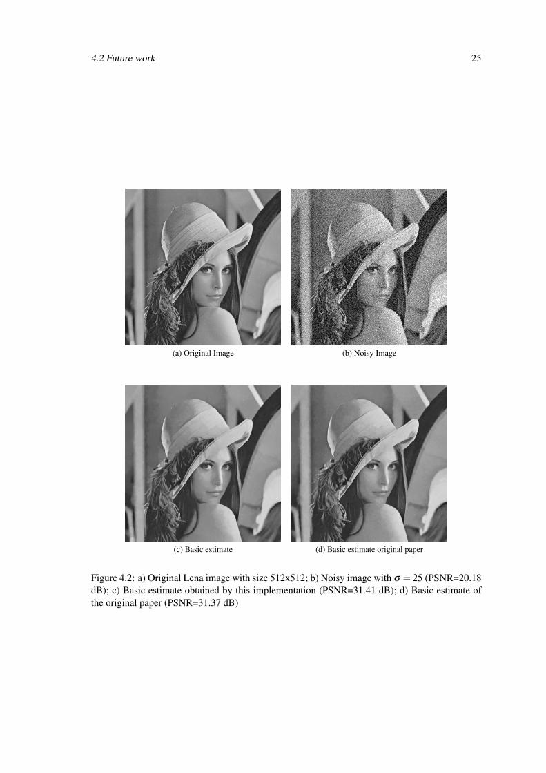
4.2 a) Original Lena image with size 512x512; b) Noisy image with σ = 25 (PSNR=20.18dB); c) Basic estimate obtained by this implementation (PSNR=31.41 dB); d) Ba-sic estimate of the original paper (PSNR=31.37 dB) . . . . . . . . . . . . . . . . 25
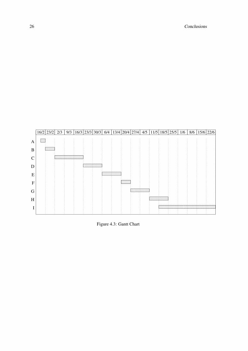
4.3 Gantt Chart . . . . . . . . . . . . . . . . . . . . . . . . . . . . . . . . . . . . . 26
v

vi LIST OF FIGURES
Abbreviations
1D One Dimension2D Two Dimensions3D Three DimensionsADC Analog to Digital ConverterAIDI Adaptive Image Denoising IP coreALU Arithmetic Logic UnitAWGN Additive White Gaussian NoiseBP Basis PursuitBM3D Block Matching and 3D FilteringCMOS Complementary Metal Oxide SemiconductorCPU Central Processing UnitCS Compressed SensingCSR Centralized Sparse RepresentationCWT Continuous Wavelet TransformDCT Discrete Cosine TransformDFT Discrete Fourier TransformDSP Digital Signal ProcessorDWT Discrete Wavelet TransformFCT Fast Cosine TransformFFT Fast Fourier TransformFPGA Field Programmable Gate Arrayfps Frames per SecondGPU Graphics Processing UnitJPEG Joint Photographic Experts GroupLUT Look-up TableMP Matching PursuitMRA Multiresolution AnalysisMSE Mean Squared ErrorNCSR Nonlocally Centralized Sparse RepresentationOMP Orthogonal Matching PursuitPCA Principle Component AnalysisPSNR Peak Signal to Noise RatioRAM Random Access MemorySAPCA Shape Adaptive Principle Component AnalysisSCN Sparse Coding NoiseSNR Signal to Noise RatioSPI Serial Peripheral InterfaceSVD Singular Value Decomposition
vii

Chapter 1
Introduction
1.1 Motivation
In the rising market of portable devices, thinness and power consumption are two main considera-
tions when producing a competitive and successful device, for example, a cell phone or a table. A
negative side effect of this constraints is a smaller camera module, which in turn has lenses with
small apertures and sensors with tiny pixels. Both these characteristics limit the amount of light
that is sensed by the camera, resulting in a reduced quality of photographs under adverse condi-
tions, such as, low light environments and small exposure times when dealing with fast moving
objects. This reduced quality appears in the image as increased motion blur, lack of contrast and
increased noise, all non-idealities that limit the accuracy of scene recognition.
Automatic scene recognition based on the information present in an image is an important
task for portable devices with many practical applications in portable devices, for example, face
detection on a smart phone. This way, the corrupted image needs to be restored in order to achieve
better results of recognition, which motivates the use of an image restoration algorithm to process
the image before the recognition task. Hence, it is of major importance to have fast and effective
restoration of an image in order to process the recognition task in real time.
The image restoration task is a heavily researched subject, with many algorithms being pro-
posed in the last years. However, most of them are highly computational demanding and take a
large amount of time to produce a restored image, when implemented in software on a general
purpose CPU. This motivates the implementation of specialized hardware to deal with a corrupted
image in real time, producing the restored image in the fastest time possible and with enhanced
quality.
In this work, a computationally inexpensive, low power and real time image denoising ap-
proach will be presented. The image denoising method enhances the quality of photographs taken
by a camera and, consequently, the accuracy for scene recognition. A novel hardware architecture
will be presented to implement the image restoration algorithm using an FPGA.
1
2 Introduction
1.2 Objectives
Image denoising algorithms can be implemented using general purpose CPUs, GPUs or special-
ized cores. The easiest solution is the implementation in a high level language such as C or C++
in a CPU, however it is also the slowest. A GPU is specialized to deal with graphics and therefore
it is more adequate to use as an image processor. On the other hand, most GPUs consume a lot of
power when faced with the kind of tasks posed by most denoising algorithms. Therefore, the best
solution is the development of a specialized core, able to denoise an image in real time and with
low power consumption, without compromising the quality of the restored image.
With the reduction of costs in the fabrication of CMOS circuits, the FPGA platforms are a very
appealing solution for the fast prototyping of novel hardware implementations. Hence, the main
objective of this work is to develop a fully specialized core for image denoising with an FPGA.
It is also an important goal that this implementation dramatically enhances the quality of images
and, hence, the quality of classification in real time, with a low power consumption.
1.3 Organization
In addition to the Introduction, this document contains three more chapters. In chapter 2 the
Background on image denoising concepts is presented. This is done in a top down approach,
starting from more general concepts and towards more specialized ones with direct applications in
the algorithm implemented. Chapter 3 follows, presenting the state of the art in image denoising
algorithms and their hardware implementations. Special emphasis is given to the algorithm chosen
to be implemented. Finally, in chapter 4, the goals achieved so far are presented, including a
preliminary implementation of the denoising algorithm in MATLAB, and the direction for future
work is defined.
Chapter 2
Background
In this chapter a simplified approach to all the concepts necessary for understanding the literature
on image denoising will be presented.
2.1 Image Denoising
In the process of capturing an image, for example, using a CMOS image sensor in a regular photo-
graphic camera, there are various constraints that influence the quality of the image produced. This
constraints generate non-idealities in the image that from a visual standpoint manifest themselves
as distortion, blur, degradation in an apparent random way (Gaussian noise), etc. The purpose of
image restoration is to restore such an image to its original content and quality.
Image Restoration is the operation of taking a corrupted/noisy image and estimating the
clean original image. Corruption may come in many forms such as motion blur, noise, and camera
misfocus. [1]
Image denoising is a method of image restoration that deals specifically with restoring an
image that has been corrupted with noise. Image noise can be defined as a random variation of
brightness or color in images produced by the components of a digital camera that intervene in the
process of forming said images. Image noise can be of the following types [2]:
• Gaussian noise: statistical random noise, that affects each pixel independently of its posi-
tion and signal intensity. It is caused primarily by Johnson-Nyquist noise (thermal noise)
coming from the signal amplifier in CMOS image sensors. This is the cause of the constant
noise level that can be seen in dark areas of an image, which is commonly known as white
noise.
• Salt and Pepper noise: a wide variety of processes that result in the same basic image
degradation are referred to as Salt and Pepper noise. This degradation occurs only for a
few pixels, but these pixels are very noisy, causing an effect similar to sprinkling white and
black dots on the image (thus the name salt and pepper). This type of noise can be caused
by ADC errors, bit errors in transmission and others.
3
4 Background
• Shot noise: also called photon counting noise, it is caused by statistical quantum variations
in the number of photons sensed at a given exposure level. Given its quantum nature, this
type of noise is always present in any imaging device, and it follows a Poisson distribution,
with an intensity proportional to the square root of the image intensity.
• Quantization noise: converting a continuous random variable to a discrete one results in
quantization noise. In images, this occurs in the acquisition process, when the pixels of a
sensed image are quantized to a number of discrete levels. This type of noise has an uniform
distribution.
• Anisotropic noise: this type of noise is, as the name states, orientation dependent and it can
cause periodic artifacts in images, visible as vertical or horizontal stripes for example.
From all the noise types the most frequent and thus the one with an increased impact in im-
age quality is Gaussian noise. Considering this, the focus of this work will be applying image
denoising in order to restore an image affected by Gaussian noise with different powers.
The classic image denoising problem can be described as follows: an ideal image y is affected
by additive zero-mean white and homogeneous Gaussian noise, n, with standard deviation σ(n).
The measured image z is given by
z(x) = y(x)+n(x), x ∈ X (2.1)
where x is a 2D spatial coordinate that belongs to the image domain X . In order to be able to
compare different image denoising algorithms, a measure of their performance must be chosen.
This can be done by computing some well known quantities, for example, the signal to noise ratio
(SNR), peak signal to noise ratio (PSNR) or mean squared error (MSE). The SNR can be defined
[3] as
SNR =σ(y)σ(n)
, (2.2)
where σ(y) denotes the empirical standard deviation of y,
σ(y) =
√1|X | ∑x∈X
(y(x)− y), (2.3)
and y is the average gray-level value. However, in order to compute the SNR it is necessary to
know beforehand the value of the standard deviation of the noise σ(n), which can only be obtained
by estimation or formally computed when the noise model is known. In order to eliminate this
dependency of the noise variance, one can use the MSE which is given by
MSE =1|X | ∑x∈X
(y(x)− y(x))2, (2.4)
where y is the estimation of the original image produced by the algorithm. It is obvious that this
measure relies on the knowledge of the original (noise free) image, which is used to evaluate and

2.2 Transform domain denoising 5
compare different algorithms in a controlled simulation where noise is added to a set of images
and applied to the algorithm. A similar measure to the MSE is the PSNR, which, assuming that
the images are normalized, is given in dB by
PSNR = 10log10
(1
|X |−1 ∑x∈X(y(x)− y(x))2
)= 10log10
(1
MSE
)(2.5)
Being specified in dB, the PSNR leads to an easier comparison of results and performance
of different algorithms, which is why it is the most commonly used measurement of denoising
performance in the literature.
In the past few years, plenty of image denoising methods were studied and created, originating
from various areas of research such as probability theory, statistics, linear and nonlinear filtering,
and spectral analysis. One common aspect shared by all these methods is that they rely on implicit
or explicit assumptions about the true image, in order to separate it properly from the noise. Two
methods that have become the state of the art in denoising, and the most researched in the past
decade, are transform domain denoising and compressed sensing based denoising.
2.2 Transform domain denoising
In natural images it is frequently observed the repetition of familiar structures and textures, which
means that the image signal is not random, and similarity between regions of an image (local
similarity) and between different regions (nonlocal similarity) occurs.
This encouraged the development of transforms that can approximate an image by linear com-
bination of few basis elements, leading to a sparse representation of the image in the transform do-
main. Therefore, when an image is affected by Gaussian noise, it is expected that in the transform
domain this noise appears as low magnitude coefficients. By discarding this small coefficients,
after applying the inverse transform, an approximation of the original image is obtained, which
means that this method can be used to effectively denoise an image.
The quality of the denoised image depends mainly on the sparsity of the representation of the
image in the transform domain. This sparsity depends on the transform used and on the original
signal properties. Obviously, the original signal can’t be controlled, so the efficiency of the de-
noising relies on the transform chosen. There are various types of transforms that can be applied
to images in order to obtain a sparse representation, but in this work there is a special interest
in evaluating two of them: the discrete wavelet transform (DWT) and the discrete cosine trans-
form (DCT). Regarding the process of discarding the small coefficients, which is usually called
shrinkage, two different methods will be presented: hard thresholding and wiener filtering.
2.2.1 Wavelets
As defined in the celebrated book of I. Daubechies, Ten Lectures on Wavelets, the wavelet trans-
form is a tool that cuts up data or functions into different frequency components, and then studies
each component with a resolution matched to its scale. [4]
6 Background
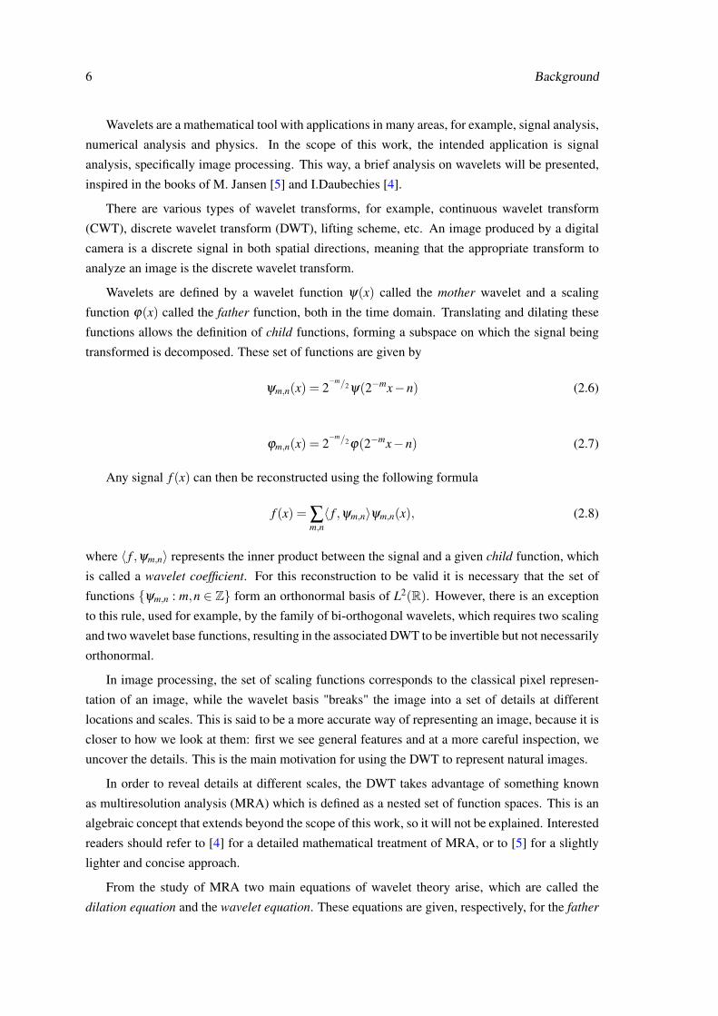
Wavelets are a mathematical tool with applications in many areas, for example, signal analysis,
numerical analysis and physics. In the scope of this work, the intended application is signal
analysis, specifically image processing. This way, a brief analysis on wavelets will be presented,
inspired in the books of M. Jansen [5] and I.Daubechies [4].
There are various types of wavelet transforms, for example, continuous wavelet transform
(CWT), discrete wavelet transform (DWT), lifting scheme, etc. An image produced by a digital
camera is a discrete signal in both spatial directions, meaning that the appropriate transform to
analyze an image is the discrete wavelet transform.
Wavelets are defined by a wavelet function ψ(x) called the mother wavelet and a scaling
function ϕ(x) called the father function, both in the time domain. Translating and dilating these
functions allows the definition of child functions, forming a subspace on which the signal being
transformed is decomposed. These set of functions are given by
ψm,n(x) = 2−m/2ψ(2−mx−n) (2.6)
ϕm,n(x) = 2−m/2ϕ(2−mx−n) (2.7)
Any signal f (x) can then be reconstructed using the following formula
f (x) = ∑m,n〈 f ,ψm,n〉ψm,n(x), (2.8)
where 〈 f ,ψm,n〉 represents the inner product between the signal and a given child function, which
is called a wavelet coefficient. For this reconstruction to be valid it is necessary that the set of
functions {ψm,n : m,n ∈ Z} form an orthonormal basis of L2(R). However, there is an exception
to this rule, used for example, by the family of bi-orthogonal wavelets, which requires two scaling
and two wavelet base functions, resulting in the associated DWT to be invertible but not necessarily
orthonormal.
In image processing, the set of scaling functions corresponds to the classical pixel represen-
tation of an image, while the wavelet basis "breaks" the image into a set of details at different
locations and scales. This is said to be a more accurate way of representing an image, because it is
closer to how we look at them: first we see general features and at a more careful inspection, we
uncover the details. This is the main motivation for using the DWT to represent natural images.
In order to reveal details at different scales, the DWT takes advantage of something known
as multiresolution analysis (MRA) which is defined as a nested set of function spaces. This is an
algebraic concept that extends beyond the scope of this work, so it will not be explained. Interested
readers should refer to [4] for a detailed mathematical treatment of MRA, or to [5] for a slightly
lighter and concise approach.
From the study of MRA two main equations of wavelet theory arise, which are called the
dilation equation and the wavelet equation. These equations are given, respectively, for the father

2.2 Transform domain denoising 7
Figure 2.1: One step of a wavelet decomposition and reconstruction. Taken from [5]
and mother functions, as
∃h ∈ `2(Z) : ϕ(x) =√
2 ∑k∈Z
hkϕ(2x− k) (2.9)
∃g ∈ `2(Z) : ψ(x) =√
2 ∑k∈Z
gkψ(2x− k) (2.10)
In the case of a bi-orthogonal basis, there are duals h and g. Given these filters, each corresponding
base function can be obtained by solving dilation and wavelet equations. An efficient realization of
the DWT can then be implemented using filter banks with the filters h, h, g and h, which are used
to decompose and reconstruct the signal, as can be seen in figure 2.1. Usually the wavelet filters
are high pass (explaining the HP in the figure), meaning they enhance details, and the scaling filters
are low pass, which means they have a smoothing effect. The filter bank DWT implementation
has the advantage that MRA becomes simply a cascading of filter banks, using the low pass output
as the new signal.
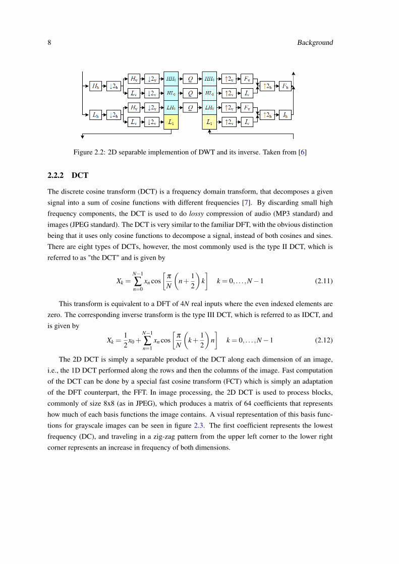
In order to analyze images, it is necessary to use a 2D DWT. This can be done by simply
applying the DWT on all rows and then on all columns of the image, which results in four types
of coefficients, or sub-bands. These sub-bands contain different image information according
to the filtering applied, for example, the HH sub-band contains diagonal features of the image,
because it corresponds to high pass filtering in both directions and the LH sub-band contains
vertical structures, corresponding to low pass filtering the columns and high pass filtering the
rows. The same logic applies to the remaining sub-bands HL and LL. A separable implementation
of the 2D DWT using filter banks can be seen in figure 2.2.
Choosing the wavelet function and the corresponding scaling function (or equivalently the
decomposition and reconstruction filters) can be a cumbersome task. To this end, the extensive
studies on wavelets originated several families of wavelet functions that are used in all wavelet
related applications. Examples of this families are the Haar-Wavelet, which is the first wavelet
ever defined; the Daubechies wavelets, Dbp with p vanishing moments; and the bi-orthogonal
wavelets BiorNd .Nr with Nd vanishing moment in the decomposition and Nr in the reconstruction.
8 Background
Figure 2.2: 2D separable implemention of DWT and its inverse. Taken from [6]
2.2.2 DCT
The discrete cosine transform (DCT) is a frequency domain transform, that decomposes a given
signal into a sum of cosine functions with different frequencies [7]. By discarding small high
frequency components, the DCT is used to do lossy compression of audio (MP3 standard) and
images (JPEG standard). The DCT is very similar to the familiar DFT, with the obvious distinction
being that it uses only cosine functions to decompose a signal, instead of both cosines and sines.
There are eight types of DCTs, however, the most commonly used is the type II DCT, which is
referred to as "the DCT" and is given by
Xk =N−1
∑n=0
xn cos[
π
N
(n+
12
)k]
k = 0, . . . ,N−1 (2.11)
This transform is equivalent to a DFT of 4N real inputs where the even indexed elements are
zero. The corresponding inverse transform is the type III DCT, which is referred to as IDCT, and
is given by
Xk =12
x0 +N−1
∑n=1
xn cos[
π
N
(k+
12
)n]
k = 0, . . . ,N−1 (2.12)
The 2D DCT is simply a separable product of the DCT along each dimension of an image,
i.e., the 1D DCT performed along the rows and then the columns of the image. Fast computation
of the DCT can be done by a special fast cosine transform (FCT) which is simply an adaptation
of the DFT counterpart, the FFT. In image processing, the 2D DCT is used to process blocks,
commonly of size 8x8 (as in JPEG), which produces a matrix of 64 coefficients that represents
how much of each basis functions the image contains. A visual representation of this basis func-
tions for grayscale images can be seen in figure 2.3. The first coefficient represents the lowest
frequency (DC), and traveling in a zig-zag pattern from the upper left corner to the lower right
corner represents an increase in frequency of both dimensions.

2.2 Transform domain denoising 9
Figure 2.3: Basis functions for a 8x8 2D DCT
2.2.3 Hard thresholding
Hard thresholding is the simplest shrinkage operator and it can be seen as a "keep or kill" procedure
[5], because all values below a certain threshold λ are set to zero, while values above the threshold
remain the same. This is given by the following expression
wλ =
w if |w| ≥ λ
0 if |w|< λ
(2.13)
A similar shrinkage operator is soft thresholding, where coefficients above the threshold are
shrunk in value by the amount of the threshold λ . This means that the soft thresholding function
is continuous, which is an advantage to some algorithms where discontinuous operators cause
problems. Plots of both operators can be seen in figure 2.4.
Figure 2.4: a) Hard thresholding operator. b) Soft thresholding operator. Adapted from [5]
10 Background
2.2.4 Wiener filtering
Wiener filtering is a statistical based approach used to produce an estimate of a target random
process, when a noisy measurement is available, as well as the signal and noise spectra. This way,
the Wiener filter minimizes MSE between the estimated process and the desired one [8]. Deriving
the expression of the Wiener filter requires a statistical approach to images. In this approach, an
image is modeled as a random noise field whose expected magnitude at each frequency is given
by [6]
E[S(wx,wy)2] = Ps(wx,wy), (2.14)
where Ps(wx,wy) is the power spectrum of the image, and E[·] denotes the expected value. Us-
ing this expression and probabilistic arguments, for example, the Bayes’ Rule, the 2D Fourier
transform of the optimum Wiener filter needed to denoise an image, can be expressed as
W (wx,wy) =Ps(wx,wy)
Ps(wx,wy)+σ2n, (2.15)
where σ2n is the power of the AWGN that corrupts the image. For interested readers, the complete
analysis to derive the Wiener filter expression can be found in [6].
2.3 Compressed Sensing based denoising
Sparse representation of signals has been a heavily researched subject in the past decade. The
brief introduction of this subject presented here is based on M. Elad’s book, Sparse and Redun-
dant Representations [9]. The main concept consists in using an overcomplete dictionary matrix
D ∈ Rn×K , containing K prototype signal atoms, to represent a signal y ∈ Rn as a sparse linear
combination of these atoms. Using this dictionary, an exact representation for the signal is given
as y = Dx. However, in many applications, an exact representation is hard to obtain, and thus, an
approximate solution is y ≈ Dx, subject to ‖y−Dx‖p ≤ ε . Measuring the approximation error is
usually done using the `p norms with p=1,2, and ∞.
When using overcomplete dictionaries, i.e., n<K, an infinite number of solutions are available
for the representation problem. This way, it is necessary to impose constraints on the solution, and
since high sparsity is desired, the solution with fewest nonzero coefficients is the most appealing.
This sparsest approximate representation is the solution of
(P0,ε) minx‖x‖0 subject to ‖y−Dx‖2 ≤ ε, (2.16)
where ‖ · ‖0 is the `0 norm, counting the nonzero entries of a vector.
As was already discussed, images can be sparsely represented using for example a wavelet
transform, leading to effective denoising algorithms using wavelets that exploit overcomplete rep-
resentations. In the case of wavelets, the dictionary is completely defined when choosing the
wavelet and scaling functions and their childs. However, in the case of compressed sensing (CS),

2.3 Compressed Sensing based denoising 11
the goal is to achieve the sparsest representation of an image in the spatial domain, i.e., the dic-
tionary has to contain the building blocks (atoms) necessary to represent any image. This requires
solving 2.16, which is proven to be an NP-hard problem [10]. Therefore, approximate solutions
to the problem are considered instead, with many approximation algorithms being proposed in the
last few years. These algorithms are in general greedy and examples are the matching pursuit (MP)
and orthogonal matching pursuit (OMP). There is also the basis pursuit (BP), which relaxes the
`0 norm in 2.16 to an `1 norm, convexifying the problem. Details about these algorithms extend
beyond the scope of this work, hence, detailed descriptions can be found, respectively in [11], [12]
and [13].
In order to develop an efficient denoising algorithm using a CS prior, the choice of dictionary
is of particular importance. For this choice there are two options: a set of pre-specified functions,
as is the case when using wavelets, DCT or other transforms; design the dictionary by adapting it
to fit a given set of signal examples, as is the case when using training based methods, such as the
PCA and K-SVD.
2.3.1 PCA
Principle component analysis (PCA) is a statistical procedure that "extracts" the principal compo-
nents of a set of observations with correlated variables using an orthogonal transformation. This
principal components are linearly uncorrelated, and thus PCA can effectively decorrelate a signal.
It was first formulated by Pearson in [14], and was further developed by Hotelling in [15].
As described in the original work of Pearson, the PCA can be seen as the line or plane that
closest fits a system of points in an n-dimensional space. Each component of the PCA "explains"
the variance in the data that the previous component is unable to fit to, i.e., the first component is
a linear combination of original variables weighted so that it represents the maximum variance in
the data, the second accounts for the variance not represented in the first, and so on.
The PCA can be used to develop a dictionary for the dataset it is applied to, so it can be used
to obtain such a dictionary that leads to a sparse representation of an image, which can then be
used to denoise said image. Usually the PCA is done by a singular value decomposition (SVD),
which means it is a highly computationally intensive method.
2.3.2 K-SVD
The K-SVD is a dictionary training algorithm, that utilizes effective sparse coding and a Gauss-
Seidel like accelerated dictionary update method. It is an extension of the popular k-means algo-
rithm, which is used to train data sets in clustering problems. The full operation of this algorithm
is complex and so, it will not be presented here. The algorithm itself is presented in figure 2.5 and
was taken from the original paper of M. Aharon, M. Elad and A. Bruckstein, K-SVD: An Algorithm
for Designing Overcomplete Dictionaries for Sparse Representation [16]. For those interested in
the algorithm, please refer to this article for a detailed explanation.

12 Background
Figure 2.5: The K-SVD algorithm. Taken from [16]
Chapter 3
Denoising Algorithms andImplementations
In this chapter some of the works found in the literature about image denoising algorithms and
some hardware implementations will be analyzed and discussed.
3.1 Image Denoising
Donoho and Johnstone were the first to explore the wavelet based denoising and the development
of the shrinkage algorithm. In their works, they applied wavelet theory to signals in general, and to
different concepts of signal processing and mathematics, such as minimax estimation [17], spatial
adaptation [18], and smooth functions [19]. In Donoho’s work [20] the shrinkage of wavelet
coefficients by applying soft thresholding is used to denoise signals. Other works using wavelet
shrinkage found in the literature are [5], [21] and [22]. The wavelet transform can be used to
form redundant representations of blocks in an image, which results in a shift invariant property,
as described in [23].
Regular wavelet transforms are not effective when representing certain image features, such
as smooth textures. This results in blurring when reconstructing or denoising an image from its
wavelet coefficients. Taking this into account, new methods to denoise an image were devel-
oped, using new multiscale and directional (anisotropic) transforms, such as the wedgelet [24],
contourlet [25], curvelet [26], bandelet [27] and steerable wavelet [28].
Dabov et. al [29] proposed in 2007 a novel method for image denoising based on collaborative
filtering in transform domain. This algorithm is called block matching and 3D filtering (BM3D)
and comprises three major steps. First, a set of similar 2D image fragments (i.e. blocks) is grouped
into 3D data arrays that are referred to as groups. This step is referred to as block matching.
Second, a 3D transform is applied to the groups, resulting in a sparse representation, that is filtered
in the transform domain, and after inversion of the transform, produces the noise-free predicted
blocks. This step is referred to as collaborative filtering. Finally, the predicted noise-free blocks are
13

14 Denoising Algorithms and Implementations
returned to their original positions to form the recovered image. BM3D relies on the effectiveness
of the block matching and collaborative filtering to produce good denoising results.
In the block matching step, blocks that are similar are grouped together in a 3D array, which
enhances the sparsity in the transform domain. This is done by matching, the process of finding
a block similar to a given reference one. The similarity of two blocks is inversely proportional to
their distance, i.e., the smaller the distance between two blocks, the more similar they are. In order
to form a group, a bound (threshold) on this distance is set, and if an `2 norm is used, this threshold
is the radius of the circle containing the blocks of the group and the reference block is the center
of this circle. The block matching is performed for every reference block in an image, using a
sliding window approach, producing a group for every block, meaning that these groups are not
necessarily disjoint, which provides an overcompleteness property. Usually, similar blocks are
only found in the same regions of an image, which motivates the restriction of searching candidate
blocks in a fixed neighborhood around the currently processed block. This restriction makes the
block matching step faster, which significantly affects the total running time of the algorithm.
The collaborative filtering comprises three steps. First a 3D (or separable 2D and 1D) trans-
form is applied to a group. Then, the transform coefficients are shrunk, by using hard thresholding
or wiener filtering in order to attenuate the noise. Finally, inverting the transform produces the
estimates for all grouped fragments. The transform takes advantage of correlation in each grouped
fragment (a peculiarity of natural images) and correlation between fragments of the same group to
produce a sparse representation of the blocks of the group, making the shrinkage very effective in
attenuating the noise. In order to reduce the complexity of applying the transforms, which results
in faster execution, 2D and 1D separable transforms are desired. This way, the transforms used
can be wavelet decompositions such as Daubechies or biorthogonal wavelets, the Haar wavelet
or the DCT. The authors compared several transforms and higher PSNR values were obtained for
the DCT transform and the bior1.5 wavelet for the 2D transform, and the Haar wavelet for the 1D
transform.
After the estimates for each block are available, they are returned to their original positions,
and because of the overcompleteness of the block matching, there can be more than one block
containing the same image pixel, i.e., overlapping. This way, in the process of aggregation, the
blocks are summed by a weighted average, using a kaiser window for reducing border effects
because of the block processing.
The BM3D algorithm is comprised of two "runs" of the aforementioned described steps. First,
the noisy image is processed using the block matching, collaborative filtering and aggregation,
using hard thresholding in the shrinkage of the transform coefficients. This produces a basic
estimate for the original noise free image. Then, using this basic estimate as input, block matching
is applied, being more accurate because the noise is already significantly attenuated. The same
groups formed in this basic estimate are formed in the original image. Then, the collaborative
filtering and aggregation is applied, but wiener filtering is used instead of hard thresholding for the
shrinkage. The wiener filter uses the basic estimate energy spectrum as the true energy spectrum
of the image, and allows for a more efficient filtering than hard thresholding, improving the final

3.1 Image Denoising 15
image quality.
Chen and Wu [30] proposed a modification to the BM3D algorithm that achieves better PSNR
and visual results for images contaminated with high levels of noise. The method is called bounded
BM3D and it differs from the original BM3D in the block matching and collaborative filtering of
the second stage of the algorithm, i.e., the basic estimate is computed in the same way to generate
a pilot signal for the second stage. The difference starts in the beginning of the second step, where
the basic estimate is partitioned into regions (image segmentation) and the boundaries between
those regions are detected. This allows for a bounded search in the block matching, i.e., only
blocks in the same image region of the reference block are candidates for grouping. However,
a block can be contained in two or more regions (coherent segments), and in this case, partial
block matching is applied, where blocks that belong to several regions are partitioned using bi-
nary masks to separate the segments. This poses a great advantage when compared to BM3D: the
partitioning avoids dealing with edges, hence avoiding problems when representing them in 3D
transform domain. Nevertheless, in order to do the wiener filtering of these non square segments,
shape adaptive DCT has to be applied as the 2D transform, which is more computationally in-
tensive. As proposed, this method achieves better PSNR, with gains of 0.23 - 1.33 dB compared
to BM3D, and better visual results, specially in edges and textures. It is worth to remark that a
similar approach was also taken by Dabov et. al in [31] with the development of shape adaptive
BM3D. Continuing this research, in [32], Dabov et. al presented an improvement to their previous
SA-BM3D algorithm, called BM3D-SAPCA, where SAPCA stands for shape adaptive principle
component analysis. The PCA is applied instead of wavelets or DCT for the 2D transform, and it
achieves better denoising results than the previous BM3D methods.
Elad and Aharon [33] devised an image denoising method based on sparse representations over
learned dictionaries. In the transform domain methods, there is also an implicit dictionary, given
by the atoms defined by the 2D DCT or a wavelet transform. However, this dictionaries, in spite of
being overcomplete, cannot represent efficiently all the information in an image. This way, Elad
and Aharon researched the possibility of using K-SVD to train a global dictionary, using a database
of noise free images. They found that for the task of image denoising, the choice of images to train
on is crucial, and while a good general dictionary that fits all images well can be found, in order to
achieve high denoising performance (comparable to BM3D and other methods), a more complex
model is necessary using several dictionaries switched by content. Therefore, in their work, they
adopted a different direction, by training the dictionary directly on the noisy image. At a first
sight, this seems to have no impact in the overall quality of the algorithm. However, Elad and
Aharon found a way to combine the denoising and training steps into the same framework. The
algorithm starts with the DCT dictionary and then performs J iterations of sparse coding followed
by dictionary training, minimizing the representation error in each iteration. The results using this
adaptive dictionary were far more promising than those using a general dictionary, which makes
this a very attractive and robust method for image denoising.
Dong et. al [34] presented a novel sparse representation model for image restoration tasks,
called centralized sparse representation (CSR). They introduce the concept of sparse coding noise

16 Denoising Algorithms and Implementations
(SCN), which is simply defined as the difference between the coding vector of the noisy image and
the coding vector of the original noise free image. However, in most cases, the original image is
not available, and so, its coding vector is not known. Nevertheless, a good estimator for this vector
is its mean value, which in turn can be approximated by the mean value of the coding vector of the
noisy image, by assuming that the SCN has nearly zero mean (which is confirmed empirically in
their work). This model is named centralized sparse representation because it enforces the coding
vector to approach its distribution center, i.e., the mean value. In order to compute the mean
value of the coding vector, groups of similar patches are created, so that their sparse codes can be
averaged, for each patch in the image. This way, the CSR model can be written as a minimization
problem, unifying the local sparsity of each patch and the nonlocal similarity induced sparsity
(from similar patches) into a variational formulation (two variable parameters control the weight of
each type of sparsity). This model can be iterated until convergence: by setting the initial estimate
for the mean value of the coding vector to zero, an initial estimate is obtained, from which the
groups are formed and the new mean value is computed and used in the following iteration. Being
a sparse representation based model, CSR relies on a dictionary, that in this work is obtained by
PCA. The CSR model converges to the desired sparse code when the joint sparse coding and non-
local clustering falls into a local minimum. Results of this method for image denoising are very
similar to those achieved by BM3D. In 2013, Dong et. al [35] proposed a modification of their
previous work on CSR, by adding the idea of nonlocality to the sparse model, allowing to remove
the local sparsity term. This way, the nonlocally centralized sparse representation (NCSR) model
achieves better denoising performance with the same computational effort.
One of the most recent works on image denoising found in the literature is by Zhong et. al
[36]. In their work a combination between the BM3D algorithm and the nonlocal centralization
prior exploited in [34] allows for very competitive results, particularly for images corrupted with
high levels of noise. The main idea is to replace the 1D transform with a shrinkage model based on
the nonlocal centralization prior. This allows the combination of the efficiency and effectiveness
of wavelet or DCT transforms (when compared with the iterated approach of the CSR model) and
the nonlocal and local sparsity unification provided by the CSR model. Moreover, the CSR model
is expanded by allowing the norms used in the shrinkage function to vary. This way, three differ-
ent shrinkage functions are proposed: one taking advantage of the `1 norm for the local sparsity
and the `2 norm for the nonlocal, other with a double `1 norm, and a final one using a nonlocal
prior to remove the local sparsity term (as proposed by [35]). In concluding remarks, essentially,
this work proposes an efficient combination of the transform domain approach for sparse repre-
sentation of images and group matching (from BM3D), with more options for advanced shrinkage
functions (based on CSR and NCSR) to replace the 1D transform and the hard thresholding or
wiener filtering used in BM3D.

3.2 Hardware Implementations 17
3.2 Hardware Implementations
Memik et. al [37],[38] were among the first to propose an FPGA implementation of an image
restoration algorithm. The algorithm used is a simple neighborhood iterative restoration algo-
rithm, that for each pixel in the image applies a convolution with a kernel that uses the eight
neighbor pixels to restore the actual pixel value. The algorithm is run for the number of iterations
necessary so that the residual is under a specified threshold, and in each iteration, all the image
pixels are processed. However, this is the software approach of the algorithm, that is very slow,
which motivates the hardware implementation in order to achieve a faster solution. The setup of
the hardware consists on a memory to store the image, a pixel processor that executes the algo-
rithm, and the channel of communication between both. Since the communication in this channel
is the bottleneck of the system, there is no gain in executing the algorithm as it is done in soft-
ware, by sending nine pixel values at a time and writing back to memory. Instead, parallelism of
the algorithm is exploited, and an array of pixel processors allows for a parallel computation of
several pixel values. Nevertheless, space in an FPGA is usually limited, and the number of pixel
processors usually is lower than the number of pixels in an image (for usual image resolutions of
256x256 or 512x512). This way, the image is segmented into regions, and each region is loaded
into the FPGA, processed, and stored back into memory. To avoid border effects and block ar-
tifacts, the segments of the image are allowed to overlap, and the overlapping restored portions
are discarded. The hardware implementation described achieves up to a ten times speedup in the
runtime of the image restoration algorithm.
Saldaña and Arias-Estrada [39] developed a reconfigurable systolic-based architecture for low
level image processing tasks on an FPGA. The architecture is tuned to allow the efficient convo-
lution of a filter kernel with an image, in a windowing based approach. The main module is a
2D customizable systolic array, with the size of the window to be used, of processing elements
(PEs). The image pixels are read from an external memory and are placed on internal memo-
ries implemented as Block RAM’s, using a Router to manage the data transfers. The 2D systolic
array is built by interconnecting several PEs, which are activated every clock cycle, following a
pipeline scheme. The PEs are specially designed in order to support the operations involved in
most window based operators, and their architecture consists of an ALU, a Shift register and an
accumulator. Each processing element executes three operations in every clock cycle: computa-
tion of the pixel value to be passed to the next cycle, accumulation of the output register calculated
at the previous cycle with the new value at the output of the ALU and loading the new mask
coefficient and transmission of the previous to the next PE. With the pipelined systolic architec-
ture, a throughput of one window output per clock cycle is achieved. Finally, the architecture was
synthesized in a Xilinx VirtexE FPGA, with a 7x7 systolic array (and corresponding sized win-
dow operation), resulting in 49 PEs and an overall area occupancy of 37%. The clock frequency
achieved was 66MHz, resulting in 200 fps for 640x480 resolution gray level images.
Joshi et. al [40] presented an FPGA implementation of a wavelet based image denoising al-
gorithm. This implementation consists of four chained main modules: the lifting scheme based
18 Denoising Algorithms and Implementations
wavelet module, the windowing module, the denoising module and the inverse wavelet module.
The first module computes the 2D DWT on the rows and columns of the image, by applying a
lifting scheme implementation of the Daubechies 9/7 biorthogonal wavelet. Each wavelet module
computes 4 rows and 4 columns at a time thanks to 4 parallel row and column modules. The
second module is the windowing module, which contains various shift registers in order to im-
plement neighborhood observation and to analyze the wavelet coefficients for the different image
sub-bands. Then, the denoising module computes the denoised coefficient, using different arith-
metic operations implemented as a 10 input squaring module, followed by a subtraction module,
a summation unit and a comparator. Finally, the inverse wavelet module applies the inverse DWT
to the denoised coefficients and stores the denoised image in the image memory. The results are
presented in terms of frames per second (fps), i.e., how many images can be denoised per second,
and the values are 83 fps for a 256x256 size image and 28 fps for 512x512.
Brylski and Strzelecki [41] proposed the implementation of a parallel image processor. The
main idea of the implementation consists of a matrix of active nodes, which correspond to the
image pixels, connected with each other by weights that depend on the neighboring pixels. The
implementation is intended to perform segmentation operations in binary images. The design con-
sists of a microcontroller connected with the PC by Ethernet and with an FPGA by SPI. The FPGA
contains a control unit and the active matrix of NxN nodes. The central unit block implements the
SPI connection and the clock manager that controls the matrix of nodes. The node block contains
several input/output signals in order to communicate with neighboring nodes, and its structure is
fairly complex. The main block is the C driver, that performs the node algorithm and controls the
work of other node unit. The complete module was synthesized in a Xilinx FPGA with 17x17
matrix elements and uses approximately 85% of the slices in the FPGA.
In the work of Di Carlo et. al [42], an adaptive image denoising IP core (AIDI) is presented,
intended for real time applications. The algorithm implemented is based on an adaptive gaussian
filter, which adapts its variance pixel by pixel according to estimates of the gaussian noise cor-
rupting the image and the local variance of the expected noise free image. This way, the AIDI
core contains three main modules: the noise variance estimator (NVE), the local variance esti-
mator (LVE) and the adaptive gaussian filter. First, the image pixels are sent in parallel to the
NVE and an external memory through a 32 bit interface, and the NVE computes the estimation
of the Gaussian noise affecting the image. Then, when this step is complete, the image is loaded
to the LVE, that computes the local variance associated with each pixel and outputs one of this
values per clock cycle, thanks to its pipelined architecture. Finally, the outputs of the LVE and
NVE are fed into the adaptive gaussian filter, which computes the optimal filter variance and then
filters the image applying Gaussian smoothing. The AIDI core was synthesized in a Xilinx Virtex
6 FPGA, occupying close to 20% of the LUTs and 1.7% of the block RAMs, and achieving 68 fps
for images with 1024x1024 pixels.
In Gabiger-Rose et. al [43], image denoising is done in real time by a bilateral filter im-
plemented in a fully synchronized architecture on an FPGA. The implementation presented has
three main advantages, enabling real time processing and effective utilization of resources: data is

3.2 Hardware Implementations 19
sorted into equal groups assigned to separate pipelines, the clock frequency is raised accordingly
to the data flow and no external image buffer is necessary. Each functional unit of the bilateral
filter consists of a register matrix, a photometric filter and a geometric filter. The register matrix
is composed by several cascaded registers and multiplexers, allowing the parallel calculation of
24 weights used by the following filter stages, and its output consists of six groups which are fed
to the photometric filter stage at four times the pixel clock. The photometric filter consists of six
identical pipelines, each processing a group of pixels at every clock cycle, and the output consists
of the weighted pixels sorted into six groups, the current center pixel being computed and the pho-
tometric coefficients for each group. The final stage is the geometric filter, that is implemented as
a separable 1D filter for the vertical and horizontal directions, and its output consists of the filtered
kernel result and a normalization factor. The normalization of the results is done by a simple divi-
sion stage at the end of the data path. The algorithm was synthesized in a Xilinx Virtex 5 FPGA,
achieving 52 fps for a 1024x1024 resolution image, and occupying 14% of slices, 23% of block
RAMs and 60% of DSP slices. In terms of the denoising results, an approximate 0.2 dB loss was
verified when comparing with the MATLAB implementation of the algorithm.

20 Denoising Algorithms and Implementations

Chapter 4
Conclusions
This chapter presents an overview of the work done so far, and sets the goals for work to be done
in the future.
4.1 Goals achieved
The main goal during the current work was to implement a preliminary version of the denoising
algorithm in an high level descriptive language, such as MATLAB. From the methods presented
in section 3.1, the algorithm chosen was the BM3D because of its high efficiency and very good
performance, with average computational burden (when compared with dictionary based meth-
ods). Starting from the original work of Dabov et al, a MATLAB implementation of the BM3D
denoising algorithm was developed. In this section, this implementation will be fully explained
and the results obtained will be compared with the original BM3D results.
The BM3D algorithm contains various parameters that are defined in the beginning of the
implementation. The parameters used were the same as presented for the normal denoising profile
in the original work. This parameters are:
• N: the block size of image patches to be processed. The value is set to N = 8.
• Nstep: the step used in the processing of reference blocks. This value is chosen to be bigger
than one in order to speedup the algorithm by a factor of approximately N2step. The value is
set to Nstep = 3.
• Nmax: this is the maximum number of blocks in each group, also decreasing the runtime of
the algorithm. This value is set to Nmax = 16 for the hard thresholding stage and Nmax = 32
for the wiener filtering stage.
• NS: the size of the neighborhood centered in the reference block from where candidate
matching blocks are searched. This value is set to NS = 39.
21
22 Conclusions
• τmatch: the threshold for group matching, i.e., blocks with distance to the reference block
under this threshold are grouped. This value is set to τmatch = 3000 for the hard thresholding
stage and τmatch = 400 for the wiener filtering stage.
• λ3D: the hard thresholding value for the first stage, which is set to λ3D = 2.7.
• β : the parameter for the Kaiser Window used to reduce border effects. This value is set to
β = 2.0.
The first step of the implementation is the pre computation of the transform domain coefficients
for every image block.
With all the parameters set, a noisy test image is created. For this, the same dataset of images is
used as in the original work. The image is read into MATLAB and normalized, i.e., the grayscale
values of [0 255] are converted to [0 1], and then a random Gaussian noise with power σ is added.
In the experiments σ was set to 25, a noise power value not too high, but already significant. The
2D transform used in the hard thresholding stage is the 2D bior1.5 wavelet, and the matrix of this
transform is hard coded. For the 1D transform, the Haar wavelet is used, and a set of transform
matrices is created. This is necessary due to the variable cardinality of the groups, that range from
1 (reference block only) to Nmax. This way, the haar wavelet transform matrices are created for
every power of 2 in the cardinality range, and when applying the 1D filter, the cardinality of the
group is rounded to the nearest lower power of 2, for example, if a group has 7 blocks, only the
first 4 blocks would be filtered.
With the noisy image created and all the transform matrices computed, the initialization of the
algorithm is done. The first step is the pre computation of the 2D transform on every possible
image block, and each block of coefficients is stored on a cell array called tBlocks. Follows the
initialization of two buffers: the image buffer which will store the filtered blocks estimates, and
the weights buffer, which stores the weights for the aggregation process.
Next, starting at the top left pixel of the image and moving Nstep pixels along direction, BM3D
is applied to each block defined by the current pixel position. For each block, group matching
is applied, searching all blocks in the neighborhood and storing the positions and distance to the
reference block of those that match. Then, the positions are ordered by ascending distance, and
the first Nmax blocks are extracted from the tBlocks array, creating a group. The next step is the
collaborative filtering, starting with determining the size of the 1D transform to use, according to
the cardinality of the group. Then, the correct 1D transform is applied to the group, producing the
3D transform domain representation of the group. Follows the actual filtering, which is performed
by hard thresholding using the previous defined threshold λ3D. Along with the filtering, the weight
for the group in the final aggregation step is computed as the inverse of the estimated noise variance
times the number of non zero coefficients left after filtering. Then, the 1D and 2D transforms are
inverted, resulting in the estimated blocks of the group. Finally, the denoised blocks are added in
the image buffer in the correct position, after multiplication by the Kaiser Window and the weight.
At the same time, the weight is added to the corresponding position in the weights buffer. When
all the image is processed, the basic estimate is obtained by simple element wise division of the

4.2 Future work 23
image buffer by the weights buffer. Figure 4.1 shows the result obtained for the basic estimate
stage for the image cameraman with size 256x256, alongside the basic estimate obtained using
the code provided by the original BM3D paper. In figure 4.2 the result for the image lena of size
512x512 is presented, along with the equivalent result of the original paper. For both images, the
basic estimate obtained by this implementation and the original paper have the same visual quality.
However, the PSNR values obtained have some differences: for the cameraman image, the PSNR
is 0.06 dB lower, and in the lena image it is 0.04 dB higher. This differences are really small, and
can be explained by different implementations of the wavelet and DCT transforms used, and by
the randomness of the Gaussian noise added to the test images.
Regarding the second stage of the algorithm, i.e., the Wiener filtering of the noisy image, the
implementation in MATLAB was complete but the results were not correct, meaning that they are
not included in this document. The next step of this work is finishing the Wiener filtering stage
with proper results, before advancing with the FPGA implementation, as will be discussed in the
following section.
4.2 Future work
With the preliminary implementation of the denoising algorithm completed, future work will focus
solely on adapting this algorithm in order to fully exploit the advantages of an hardware oriented
implementation. This will begin by correcting and tuning the algorithm in MATLAB, in order to
make all the code synthesizable when advancing to the hardware architecture. The next step is
exactly this, development and simulation of the hardware architecture, which is expected to be the
most demanding and time consuming task of the future work. Next follows the synthesis of the
hardware and preliminary testing and tuning on an FPGA. The final step is the assessment of the
system with real images. The time for each of this tasks and the planing is presented as a Gantt
chart in figure 4.3. Due to limited space, the tasks in the chart are simply labeled A to I. These
tasks are the following:
• Task A: MATLAB Implementation.
• Task B: Setup development environment.
• Task C: Verilog - System development.
• Task D: Verilog - System simulation.
• Task E: Verilog - Design synthesis.
• Task F: Testing and tuning on FPGA.
• Task G: Final System testing.
• Task H: Optimization.
• Task I: Dissertation Writing.

24 Conclusions
(a) Original Image (b) Noisy Image
(c) Basic estimate (d) Basic estimate original paper
Figure 4.1: a) Original Cameraman image with size 256x256; b) Noisy image with σ = 25(PSNR=20.17 dB); c) Basic estimate obtained by this implementation (PSNR=29.08 dB); d) Basicestimate of the original paper (PSNR=29.14 dB)
4.2 Future work 25
(a) Original Image (b) Noisy Image
(c) Basic estimate (d) Basic estimate original paper
Figure 4.2: a) Original Lena image with size 512x512; b) Noisy image with σ = 25 (PSNR=20.18dB); c) Basic estimate obtained by this implementation (PSNR=31.41 dB); d) Basic estimate ofthe original paper (PSNR=31.37 dB)
26 Conclusions
16/2 23/2 2/3 9/3 16/3 23/3 30/3 6/4 13/4 20/4 27/4 4/5 11/5 18/5 25/5 1/6 8/6 15/6 22/6
A
B
C
D
E
F
G
H
I
Figure 4.3: Gantt Chart
References
[1] S Asha, S Bhuvana, and R Radhakrishnan. A Survey on Content Based Image RetrievalBased on Feature Extraction. Int. J. Novel. Res. Eng & Pharm. Sci, 1(06):29–34, 2014.
[2] Alan C. Bovik. Handbook of Image and Video Processing. Academic Press, 2010.
[3] A Buades, B Coll, and J Morel. A Review of Image Denoising Algorithms, with a New One.Multiscale Modeling & Simulation, 4(2):490–530, 2005.
[4] I Daubechies. Ten Lectures on Wavelets. Society for Industrial and Applied Mathematics,1992.
[5] Maarten Jansen. Noise Reduction by Wavelet Thresholding, volume 161 of Lecture Notes inStatistics. Springer New York, New York, NY, 2001.
[6] Richard Szeliski. Computer vision: algorithms and applications. 2010.
[7] N. Ahmed, T. Natarajan, and K.R. Rao. Discrete Cosine Transform. IEEE Transactions onComputers, C-23(1):90–93, January 1974.
[8] Robert Grover Brown and Patrick Y. C. Hwang. Introduction to Random Signals and AppliedKalman Filtering. John Wiley & Sons, 2012.
[9] Michael Elad. Sparse and Redundant Representations: From Theory to Applications inSignal and Image Processing. 2010.
[10] G. Davis, S. Mallat, and M. Avellaneda. Adaptive greedy approximations. ConstructiveApproximation, 13(1):57–98, March 1997.
[11] S.G. Mallat. Matching pursuits with time-frequency dictionaries. IEEE Transactions onSignal Processing, 41(12):3397–3415, 1993.
[12] Y.C. Pati, R. Rezaiifar, and P.S. Krishnaprasad. Orthogonal matching pursuit: recursivefunction approximation with applications to wavelet decomposition. In Proceedings of 27thAsilomar Conference on Signals, Systems and Computers, pages 40–44. IEEE Comput. Soc.Press, 1993.
[13] Scott Shaobing Chen, David L. Donoho, and Michael A. Saunders. Atomic Decompositionby Basis Pursuit. SIAM Journal on Scientific Computing, 20(1):33–61, January 1998.
[14] K Pearson. On lines and planes of closest fit to systems of points in space. PhilosophicalMagazine, 2(6):559 – 572, 1901.
[15] H. Hotelling. Analysis of a complex of statistical variables into principal components. Jour-nal of Educational Psychology, 24(6):417–441, 1933.
27

28 REFERENCES
[16] M. Aharon, M. Elad, and A. Bruckstein. K-SVD: An Algorithm for Designing Overcom-plete Dictionaries for Sparse Representation. IEEE Transactions on Signal Processing,54(11):4311–4322, November 2006.
[17] David L. Donoho and Iain M. Johnstone. Minimax estimation via wavelet shrinkage. TheAnnals of Statistics, 26(3):879–921, June 1998.
[18] David L. Donoho and Iain M. Johnstone. Ideal spatial adaptation by wavelet shrinkage.Biometrika, 81(3):425–455, September 1994.
[19] David L. Donoho and Iain M. Johnstone. Adapting to Unknown Smoothness via WaveletShrinkage. Journal of the American Statistical Association, 90(432):1200–1224, February1995.
[20] D.L. Donoho. De-noising by soft-thresholding. IEEE Transactions on Information Theory,41(3):613–627, May 1995.
[21] A Charnbolle, R A DeVore, N Y Lee, and B J Lucier. Nonlinear wavelet image processing:variational problems, compression, and noise removal through wavelet shrinkage. IEEEtransactions on image processing : a publication of the IEEE Signal Processing Society,7(3):319–35, January 1998.
[22] P. Moulin. Analysis of multiresolution image denoising schemes using generalized-Gaussianpriors. In Proceedings of the IEEE-SP International Symposium on Time-Frequency andTime-Scale Analysis (Cat. No.98TH8380), pages 633–636. IEEE, 1998.
[23] D. L. Donoho and R. R. Coifman. Translation invariant denoising. In Wavelets and Statistics,pages 125–150. Springer-Verlag New York, New York, NY, 1995.
[24] David L. Donoho. Wedgelets: nearly minimax estimation of edges. The Annals of Statistics,27(3):859–897, June 1999.
[25] Minh Do and Martin Vetterli. Contourlets. In Beyond Wavelets, pages 1–27. Academic Press,New York, NY, 2001.
[26] Emmanuel J Candès and David L Donoho. New tight frames of curvelets and optimal repre-sentations of objects with piecewise C2 singularities. Communications on Pure and AppliedMathematics, 57(2):219–266, 2004.
[27] E. Le Pennec and S. Mallat. Sparse geometric image representations with bandelets. IEEETransactions on Image Processing, 14(4):423–438, April 2005.
[28] W.T. Freeman and E.H. Adelson. The design and use of steerable filters. IEEE Transactionson Pattern Analysis and Machine Intelligence, 13(9):891–906, 1991.
[29] K. Dabov, A. Foi, V. Katkovnik, and K. Egiazarian. Image Denoising by Sparse 3-D Transform-Domain Collaborative Filtering. IEEE Transactions on Image Processing,16(8):2080–2095, August 2007.
[30] Qian Chen and Dapeng Wu. Image denoising by bounded block matching and 3D filtering.Signal Processing, 90(9):2778–2783, September 2010.
[31] K Dabov, A Foi, V Katkovnik, and K Egiazarian. A nonlocal and shape-adaptive transform-domain collaborative filtering. . . . Int. Workshop on Local and Non . . . , 2008.

REFERENCES 29
[32] K Dabov, A Foi, V Katkovnik, and K Egiazarian. BM3D image denoising with shape-adaptive principal component analysis. SPARS’09-Signal Processing . . . , 2009.
[33] Michael Elad and Michal Aharon. Image Denoising Via Sparse and Redundant Represen-tations Over Learned Dictionaries. IEEE Transactions on Image Processing, 15(12):3736–3745, December 2006.
[34] Weisheng Dong, Lei Zhang, and Guangming Shi. Centralized sparse representation for im-age restoration. In 2011 International Conference on Computer Vision, pages 1259–1266.IEEE, November 2011.
[35] Weisheng Dong, Lei Zhang, Guangming Shi, and Xin Li. Nonlocally centralized sparserepresentation for image restoration. IEEE transactions on image processing : a publicationof the IEEE Signal Processing Society, 22(4):1620–30, April 2013.
[36] Hua Zhong, Ke Ma, and Yang Zhou. Modified BM3D algorithm for image denoising usingnonlocal centralization prior. Signal Processing, 106:342–347, January 2015.
[37] S.O. Memik, K. Bazargan, and M. Sarrafzadeh. Image analysis and partitioning for FPGAimplementation of image restoration. In 2000 IEEE Workshop on SiGNAL PROCESSINGSYSTEMS. SiPS 2000. Design and Implementation (Cat. No.00TH8528), pages 346–355.IEEE, 2000.
[38] S.O. Memik, A.K. Katsaggelos, and M. Sarrafzadeh. Analysis and FPGA implementation ofimage restoration under resource constraints. IEEE Transactions on Computers, 52(3):390–399, March 2003.
[39] G. Saldana and M. Arias-Estrada. FPGA-Based Customizable Systolic Architecture for Im-age Processing Applications. In 2005 International Conference on Reconfigurable Comput-ing and FPGAs (ReConFig’05), pages 3–3. IEEE, 2005.
[40] Jonathan Joshi, Nisseem Nabar, and Parul Batra. Reconfigurable Implementation of Waveletbased Image Denoising. In 2006 49th IEEE International Midwest Symposium on Circuitsand Systems, volume 1, pages 475–478. IEEE, August 2006.
[41] P. Brylski and M. Strzelecki. FPGA implementation of parallel digital image processor. InSignal Processing Algorithms, Architectures, Arrangements, and Applications ConferenceProceedings (SPA), 2010, pages 25–28, 2010.
[42] Stefano Di Carlo, Paolo Prinetto, Daniele Rolfo, and Pascal Trotta. AIDI: An adaptive imagedenoising FPGA-based IP-core for real-time applications. In 2013 NASA/ESA Conferenceon Adaptive Hardware and Systems (AHS-2013), pages 99–106. IEEE, June 2013.
[43] Anna Gabiger-Rose, Matthias Kube, Robert Weigel, and Richard Rose. An FPGA-BasedFully Synchronized Design of a Bilateral Filter for Real-Time Image Denoising. IEEE Trans-actions on Industrial Electronics, 61(8):4093–4104, August 2014.