Algorithmic Composition:The Music of Mathematics

Carlo AnselmoAnselmoC18@hsc.edu

May 8, 2018

Abstract

We report on several techniques we have developed for generating musical

compositions algorithmically. Most of our techniques are based on our idea of

a sequence recursion, which is a method for generating finite integer sequences

that can represent pitches and rhythms. Our research is two-pronged: we de-

velop the mathematical properties and techniques associated with sequence

recursions, and we apply these techniques to the synthesis of new musical

compositions. Sequence recursions use basic musical operations such as rep-

etition, transposition, and inversion to iteratively generate integer sequences

of increasing length and complexity. These sequences are then mapped into

musical structures such as scale or rhythm patterns to produce melodies and

accompaniments. We present several examples of musical compositions pro-

duced by this process.

1 Introduction

In this paper, we report on several techniques we have developed for generating mu-sical compositions algorithmically. These techniques are based primarily on our ideaof a sequence recursion, which is a method for generating finite integer sequencesthat can represent pitches and rhythms. We call these sequences pitch patterns andrhythm patterns, respectively, and we have developed many operations we can per-form on them. Pitch patterns provide a list of integers that are mapped onto pitches,while rhythm patterns designate the start times for notes. Rhythm patterns alsohave a corresponding object called a division scheme, which dictates the interval oftime a rhythm pattern lives on. For both pitch and rhythm, some of the operationswe have developed mirror basic musical operations such as repetition, transposition,and inversion when we iteratively generate sequences of increasing length and com-plexity. However, we also have a number of operations that are unusual in standardmusical composition, and yield interesting and unexpected results. For both pitchesand rhythms, these unusual operations are rotation, reversal, concatenation, andcomposition, and rhythm patterns additionally use the merge operation. Modernmusical notation utilizes notes, which are objects that contain information about

1

both pitch and duration. In this case, pitch and rhythm are intrinsically lockedtogether, but in our research, information about pitch and rhythm are stored in twoseparate sequences, and we later tie them both together into one object, which wecall a melody/line.

Our research is two-pronged: we develop the mathematical properties and tech-niques associated with sequence recursions, and we apply these techniques to thesynthesis of new musical compositions. Our primary tool for sequence recursions issomething we call a substitution scheme, and in our research, we have thoroughly ex-plored the uses and properties of these schemes. Substitution schemes take shorter,simpler pitch and rhythm patterns, and transform them into into longer and morecomplicated sequences. We also present two special cases of substitution schemes,called palindromic and rearrangement schemes.

When synthesizing new compositions, we utilize our algorithmic techniques togenerate both melody and harmony. We usually only focus on designing melody,because harmony and accompaniments naturally arise out of the melody we create.We also take into consideration a musician’s needs for sheet music, and we have de-signed a number of methods for performing mathematical tweaks on music to makeit more playable, including transposition, modulo, and reflection. We present severalexamples of musical compositions produced by this process.

This primary mathematical focus of this research is on pitch and its related com-ponents. Though we do not delve too deeply into the mathematics of rhythm, wehave developed enough theory to at least utilize it in the creation of music [3]. Ad-ditionally, the two other primary aspects of music, volume and timbre, are selectedarbitrarily—however, we could certainly determine these parameters algorithmicallyas well.

2 Theory and Methods

2.1 Pitch

We will first discuss pitch and a mathematical way to model it. Musical pitch refersto the quality of sound governed by the rate of vibrations producing it. In termsof human perception, we are talking about the degree of highness or lowness of atone. Without getting into too much detail, distinct pitches in musical notation aredenoted by the letters A to G. Notes increase in pitch as one would expect, suchthat a C sounds lower than a D, and so on.

2.1.1 Pitch Patterns

Core to this research is the idea that musical pitches can be represented with inte-gers. For example, we could arbitrarily map the integers 0, 1, and 2 to the notes C,C#, and D, respectively. In order to meet these specifications, we combine strings ofintegers into an object we have created called a pitch patterns, which we directlytransform into sequences of musical notes. We denote the set of all pitch patternsby P =

S1n=1 Zn, where Z is the set of all integers. Throughout this paper, we will

2

use letters from the first half of the Greek alphabet to denote pitch patterns.As a side note, an octave is an interval between one musical pitch and another

with a frequency that di↵ers by a power of two. The note that is an octave abovea C is still called a C, but we say it is in a higher octave. There are twelve tonesbetween an octave in standard western music, although there are an infinite numberof frequencies. In our research, we rely on octaves through our notion of octaveequivalence, which we define as the ability to move between di↵erent octaves of apitch without changing the fundamental sound of a musical composition. Whenfaced with a pitch pattern with a large range of integers, we utilize octave equiva-lence to continue notes as far upwards or downwards as desired.

2.1.2 Pitch Pattern Operations

We outline a number of useful operations we have created in order to manipulatepitch patterns. The first is transposition. The transposition of a pitch pattern ↵ ofsize m by k 2 Z scale steps is denoted by k+↵, and the addition is component-wise:

k + ↵ = (k + ↵0, k + ↵1, . . . , k + ↵m�1).

The second is inversion. Inversion of ↵ about 0 is given by �↵, while the inversionabout k is 2k � ↵.

Third is rotation. Rotation is circular, and we denote the rotation of ↵ as �k↵,where a positive k represents the number of steps ↵ is rotated to the right, and anegative k signals a left rotation of k steps.

The fourth operation—reversal—is denoted by ↵, and reversing the order of theelements in ↵ gives

↵ = (↵m�1,↵m�2, . . . ,↵0).

Additionally, we utilize two binary operations for pitch patterns, the first beingconcatenation. Given pitch patterns ↵ and � of length m and n, respectively, theconcatenation of ↵ followed by � is defined by

(↵, �) = (↵0 ↵1 . . . ↵m�1, �0 �1 . . . �n�1).

The second is composition. Let ↵ and � be pitch patterns with lengths m and n,respectively. The composition ↵� is the pitch pattern of length mn given by

↵� = (↵0 + �, ↵1 + �, . . . ,↵m�1 + �) .

3

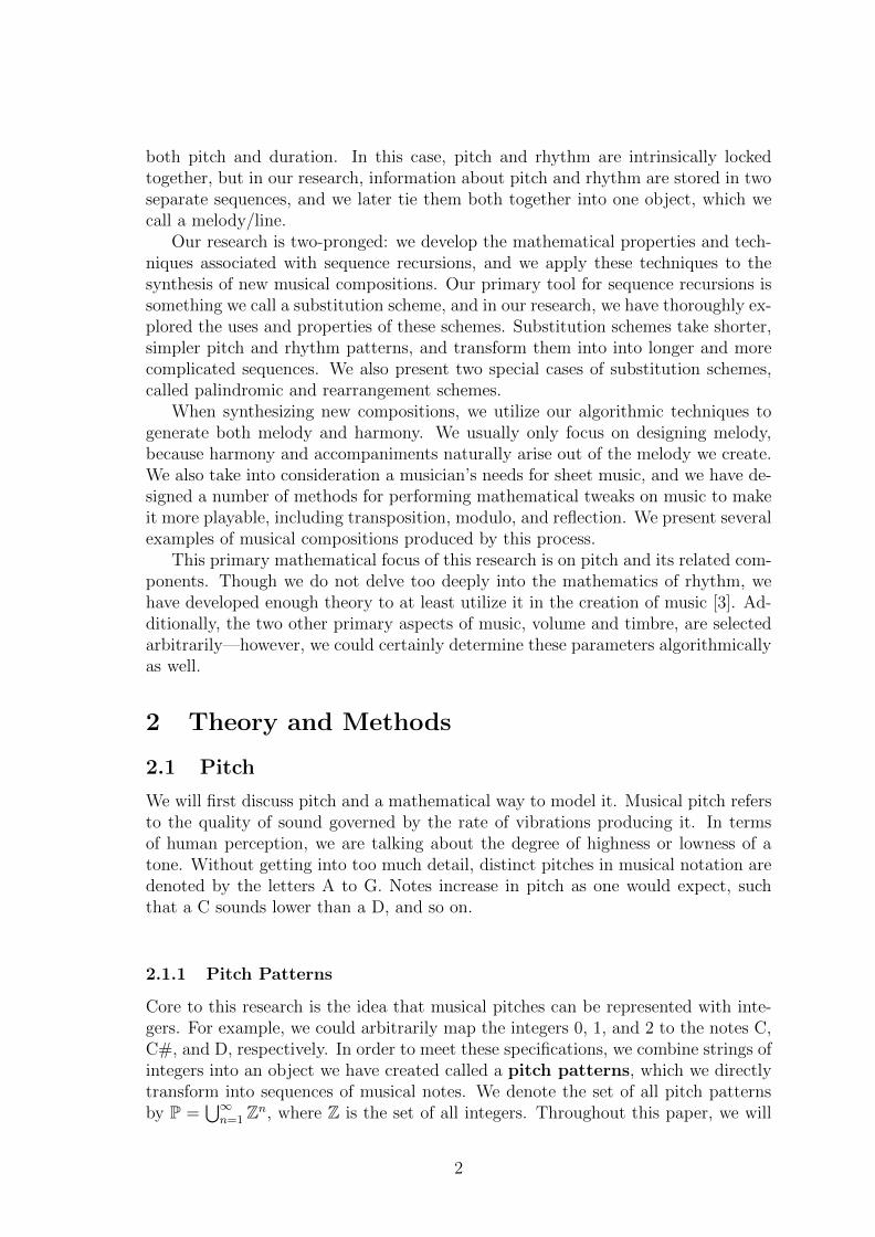
For example, let ↵ = (2 0 1) and � = (1 0). We may represent these patterns usingthe following step diagrams.

0

1

2�

�

�

Pattern ↵

0

1

2

↵

↵

Pattern �

Figure 1: Step diagrams of ↵ and �.

Then

↵� = (↵0 + �,↵1 + �,↵2 + �)

= (2 + (1 0), 0 + (1 0), 1 + (1 0))

= (3 2 1 0 2 1)

and

�↵ = (�0 + ↵, �1 + ↵)

= (1 + (2 0 1), 0 + (2 0 1))

= (3 1 2 2 0 1).

Note that ↵� 6= �↵. The composition of pitch patterns is often not commutative,meaning ↵� 6= �↵. However, it is associative, such that (↵�)� = ↵(��) [2]. We callthe pitch pattern (0) the identity element for composition, since (0)� = �(0) = �for all pitch patterns �.

Additionally, note that powers of composition take the following form:

↵ = (↵0, ↵1, . . . , ↵m�1)

↵↵ = (↵0 + ↵, ↵1 + ↵, . . . , ↵m�1 + ↵)

↵3 = ((↵↵)0 + ↵, (↵↵)1 + ↵, . . . , (↵↵)m2�1 + ↵)

= (↵20 + ↵, ↵2

1 + ↵, . . . , ↵2m2�1 + ↵)

↵n+1 =�↵n0 + ↵, ↵n

1 + ↵, . . . , ↵nmn�1 + ↵

�

The following theorem highlights some properties of composition.

Theorem 2.1. Let ↵ and � be pitch patterns, and let c, d, j, k, and n be integralconstants. Then the following properties of compositions hold:

1. (k + ↵)(j + �) = (k + j) + ↵�.

2. (k + ↵)n = kn+ ↵n.

4

3. (c↵)n = c↵n.

4. (c↵)(j + �) = j + c↵�.

5. (k + ↵)(d�) = k + d↵�.

Proof.

1. We have

(k + ↵)(j + �) = ((k + ↵0) + (j + �), (k + ↵1) + (j + �), . . . , (k + ↵m�1) + (j + �))

= ((k + j) + (↵0 + �), (k + j) + (↵1 + �), . . . , (k + j) + (↵m�1 + �))

= (k + j) + (↵0 + �,↵1 + �, . . . ,↵m�1 + �)

= (k + j) + ↵�.

2. (Base) When n = 1, (k + ↵)1 = k + ↵ = k(1) + ↵.(Inductive step) We assume (k + ↵)p = kp + ↵p for some p, and we need toshow that (k + ↵)p+1 = k(p+ 1) + ↵p+1 for all p. Then

(k + ↵)p+1 = (k + ↵)(k + ↵)p

= (k + ↵)(kp+ ↵p) (By the inductive assumption)

= k(p+ 1) + ↵p+1. (By 1.)

3. (Base) When n = 1, (c↵)1 = c↵.(Inductive step) We assume (c↵)p = c↵p for some p, and we need to show that(c↵)p+1 = c↵p+1 for all p. Then

(c↵)p+1 =�(c↵)p0 + c↵, (c↵)p1 + c↵, . . . , (c↵)pmp�1 + c↵

�(By the note above)

=�c↵p

0 + c↵, c↵p1 + c↵, . . . , c↵p

mp�1 + c↵�

(By the inductive assumption)

=�c(↵p

0 + ↵), c(↵p1 + ↵), . . . , c(↵p

mp�1 + ↵)�

= c�↵p0 + ↵,↵p

1 + ↵, . . . ,↵pmp�1 + ↵

�

= c↵p+1. (By the note above)

4. Note that

(c↵)(j + �) = ((c↵0) + (j + �), (c↵1) + (j + �), . . . , (c↵m�1) + (j + �))

= j + (c↵0 + �, c↵1 + �, . . . , c↵m�1 + �)

= j + c↵�.

5. Observe that

(k + ↵)(d�) = ((k + ↵0) + (d�), (k + ↵1) + (d�), . . . , (k + ↵m�1) + (d�))

= k + (↵0 + d�,↵1 + d�, . . . ,↵m�1 + d�)

= k + d↵�.

⌅This theorem is by no means exhaustive, but for our purposes, we will utilize onlythe operations given above when generating pitch patterns.

5

2.2 Rhythm

In addition to pitches, rhythms may also be represented mathematically. In musictheory, a beat is the basic unit of time; it is often defined as the numbers a musicianwould count while performing. A note may last any number of beats, and each notehas a name with respect to its duration. In most cases, a whole note refers to a notewhich lasts four beats. Intuitively, a half note refers to a note with a duration oftwo beats, a quarter note to one beat, an eighth note to a half a beat, and so on. Ameasure is a segment of time corresponding to a specific number of beats. Dividingmusic into measures provides regularity in a musical composition, a regularity thathelps analyze music in a more mathematical fashion. A time signature defines howmany beats occur in a measure, as well as which note receives the beat. One finalaspect of interest for rhythms is the accent, which describes a particular emphasisplaced on a note. Generally, greater emphasis is placed on higher-level beats, whilegreater subdivisions receive a decreasing amount of emphasis.

Though our research does not heavily focus on the mathematical representa-tion of rhythm, we still work with the conceptual properties of rhythm and exploremethods for generating new rhythms.

2.2.1 Division Schemes

We first define our method of subdividing time into regular intervals, following [3].A division scheme is a division of an interval into d`�1 equal subintervals, each ofwhich is subdivided into d`�2 equal subintervals, and so on, concluding with a finalsubdivision of each interval into d0 equal subintervals. Division schemes take theform D = (d`�1 d`�2 . . . d1 d0), where ` is the number of levels in the scheme, andthe value of di is the number of subdivisions at level i. Beats are numbered fromzero. We typically interpret the levels in divisions schemes as how much emphasisa particular beat receives, with the leftmost level receiving the most emphasis, andthe rightmost level receiving the least.

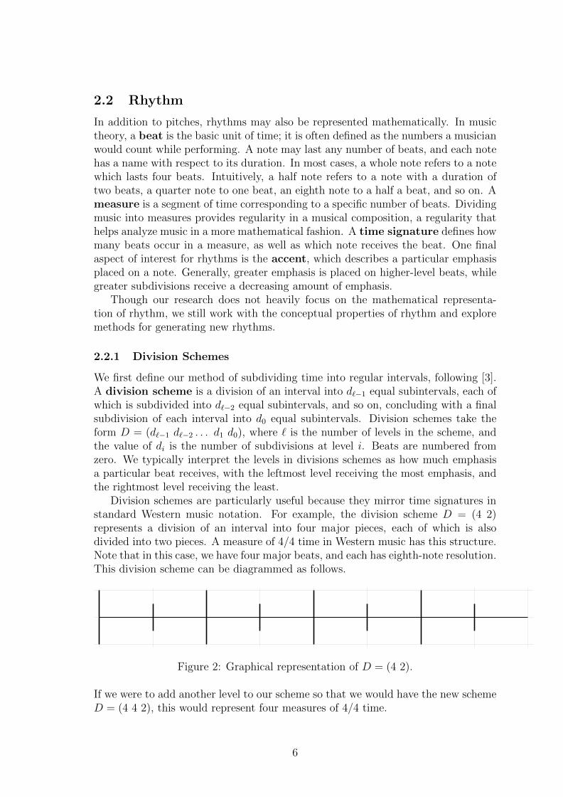
Division schemes are particularly useful because they mirror time signatures instandard Western music notation. For example, the division scheme D = (4 2)represents a division of an interval into four major pieces, each of which is alsodivided into two pieces. A measure of 4/4 time in Western music has this structure.Note that in this case, we have four major beats, and each has eighth-note resolution.This division scheme can be diagrammed as follows.

Figure 2: Graphical representation of D = (4 2).

If we were to add another level to our scheme so that we would have the new schemeD = (4 4 2), this would represent four measures of 4/4 time.

6

2.2.2 Rhythm Patterns

As with pitch patterns, we have developed a way to organize rhythms systematically.We define a rhythm pattern as a sequence of strictly increasing positive integersthat represent the starting times for a sequence of notes. Unless we specify dura-tion, one note is played up until the starting time of a new note. We denote rhythmpatterns with letters from the second half of the Greek alphabet. An example ofa perfectly reasonable rhythm pattern is (0 1 2 3), which signifies four notes heldfor equal durations. The purpose of divisions schemes are to contextualize rhythmpatterns in an interval of time, and they are particularly useful at illustrating morecomplicated rhythm patterns. Division schemes also inform us when the last noteof a rhythm pattern ends.

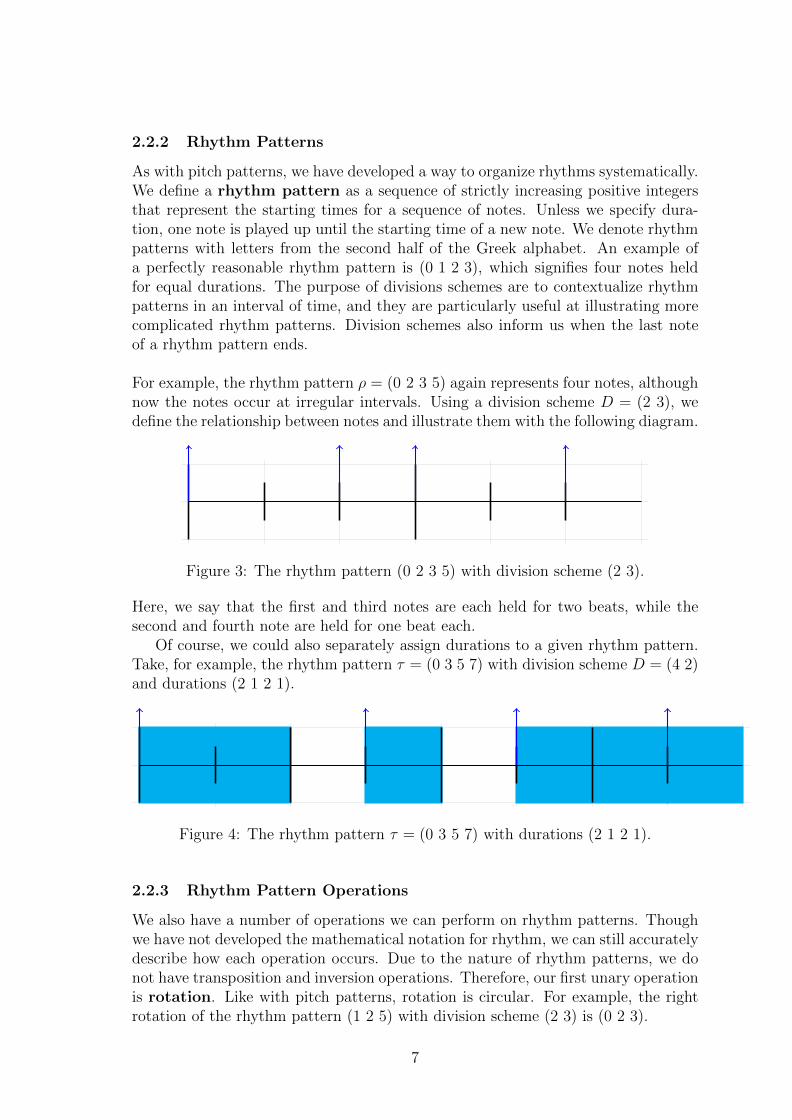
For example, the rhythm pattern ⇢ = (0 2 3 5) again represents four notes, althoughnow the notes occur at irregular intervals. Using a division scheme D = (2 3), wedefine the relationship between notes and illustrate them with the following diagram.

Figure 3: The rhythm pattern (0 2 3 5) with division scheme (2 3).

Here, we say that the first and third notes are each held for two beats, while thesecond and fourth note are held for one beat each.

Of course, we could also separately assign durations to a given rhythm pattern.Take, for example, the rhythm pattern ⌧ = (0 3 5 7) with division scheme D = (4 2)and durations (2 1 2 1).

Figure 4: The rhythm pattern ⌧ = (0 3 5 7) with durations (2 1 2 1).

2.2.3 Rhythm Pattern Operations

We also have a number of operations we can perform on rhythm patterns. Thoughwe have not developed the mathematical notation for rhythm, we can still accuratelydescribe how each operation occurs. Due to the nature of rhythm patterns, we donot have transposition and inversion operations. Therefore, our first unary operationis rotation. Like with pitch patterns, rotation is circular. For example, the rightrotation of the rhythm pattern (1 2 5) with division scheme (2 3) is (0 2 3).

7

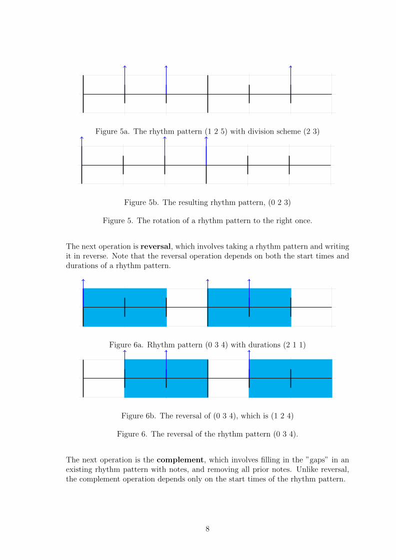
Figure 5a. The rhythm pattern (1 2 5) with division scheme (2 3)

Figure 5b. The resulting rhythm pattern, (0 2 3)

Figure 5. The rotation of a rhythm pattern to the right once.

The next operation is reversal, which involves taking a rhythm pattern and writingit in reverse. Note that the reversal operation depends on both the start times anddurations of a rhythm pattern.

Figure 6a. Rhythm pattern (0 3 4) with durations (2 1 1)

Figure 6b. The reversal of (0 3 4), which is (1 2 4)

Figure 6. The reversal of the rhythm pattern (0 3 4).

The next operation is the complement, which involves filling in the ”gaps” in anexisting rhythm pattern with notes, and removing all prior notes. Unlike reversal,the complement operation depends only on the start times of the rhythm pattern.

8

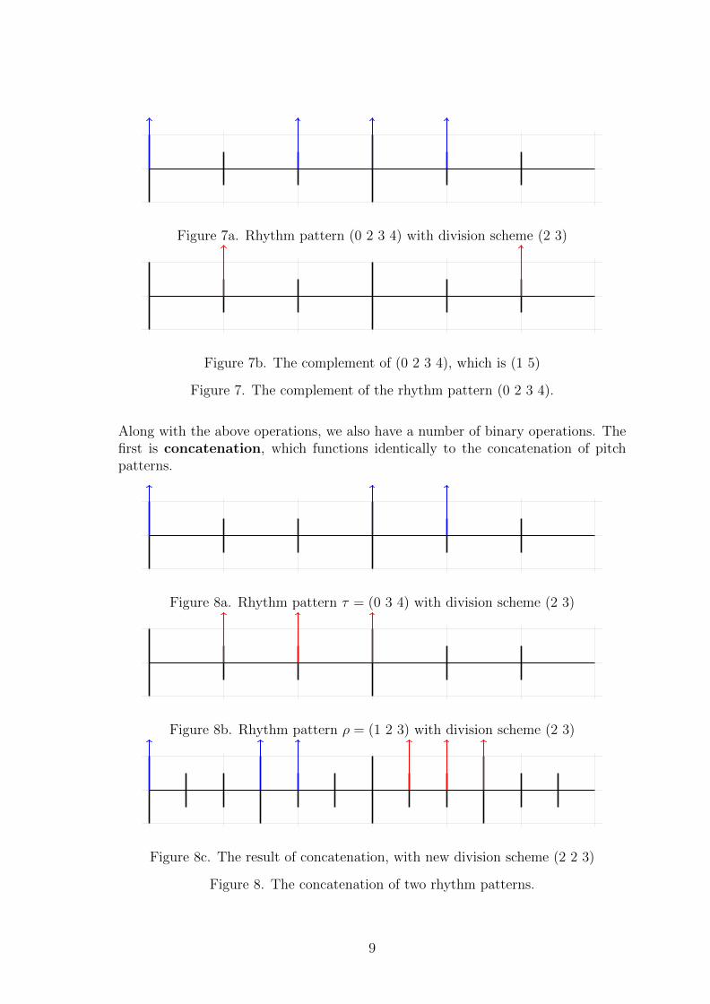
Figure 7a. Rhythm pattern (0 2 3 4) with division scheme (2 3)

Figure 7b. The complement of (0 2 3 4), which is (1 5)

Figure 7. The complement of the rhythm pattern (0 2 3 4).

Along with the above operations, we also have a number of binary operations. Thefirst is concatenation, which functions identically to the concatenation of pitchpatterns.

Figure 8a. Rhythm pattern ⌧ = (0 3 4) with division scheme (2 3)

Figure 8b. Rhythm pattern ⇢ = (1 2 3) with division scheme (2 3)

Figure 8c. The result of concatenation, with new division scheme (2 2 3)

Figure 8. The concatenation of two rhythm patterns.

9

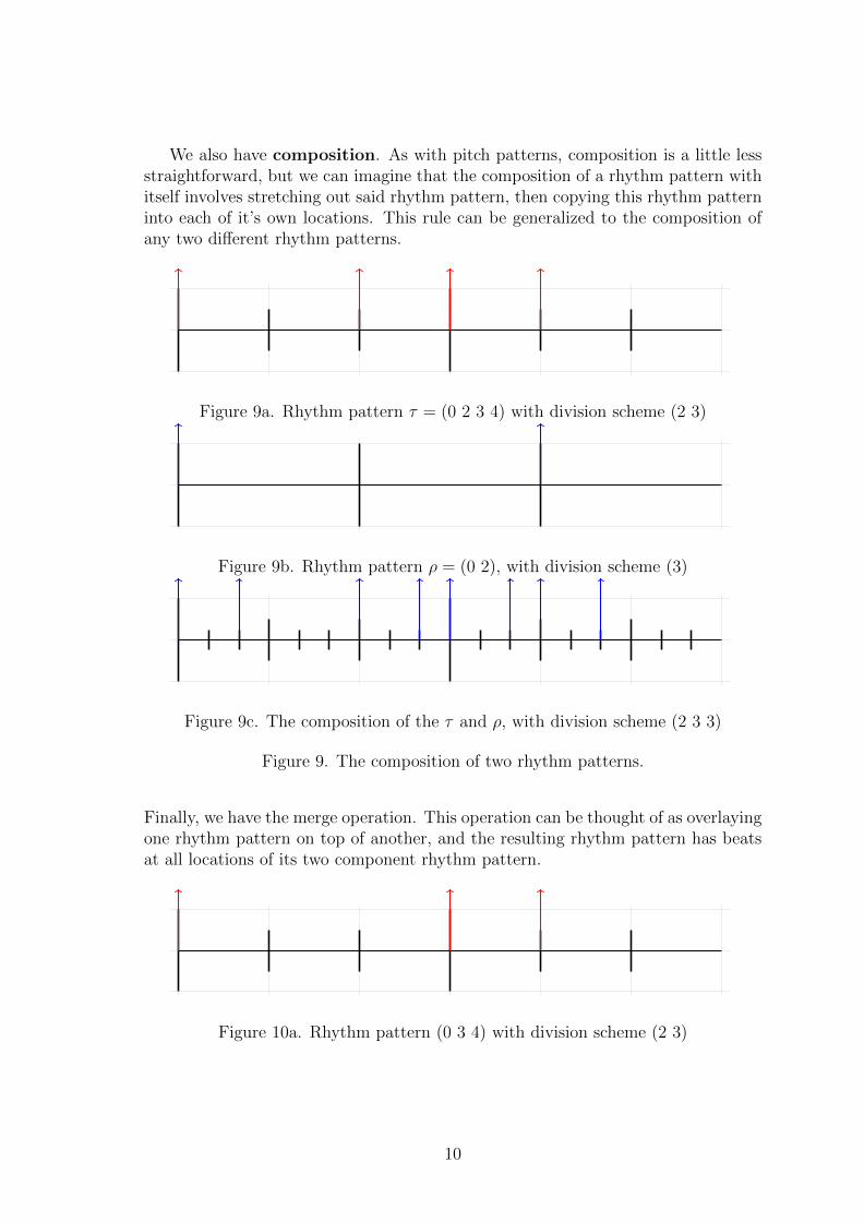
We also have composition. As with pitch patterns, composition is a little lessstraightforward, but we can imagine that the composition of a rhythm pattern withitself involves stretching out said rhythm pattern, then copying this rhythm patterninto each of it’s own locations. This rule can be generalized to the composition ofany two di↵erent rhythm patterns.

Figure 9a. Rhythm pattern ⌧ = (0 2 3 4) with division scheme (2 3)

Figure 9b. Rhythm pattern ⇢ = (0 2), with division scheme (3)

Figure 9c. The composition of the ⌧ and ⇢, with division scheme (2 3 3)

Figure 9. The composition of two rhythm patterns.

Finally, we have the merge operation. This operation can be thought of as overlayingone rhythm pattern on top of another, and the resulting rhythm pattern has beatsat all locations of its two component rhythm pattern.

Figure 10a. Rhythm pattern (0 3 4) with division scheme (2 3)

10

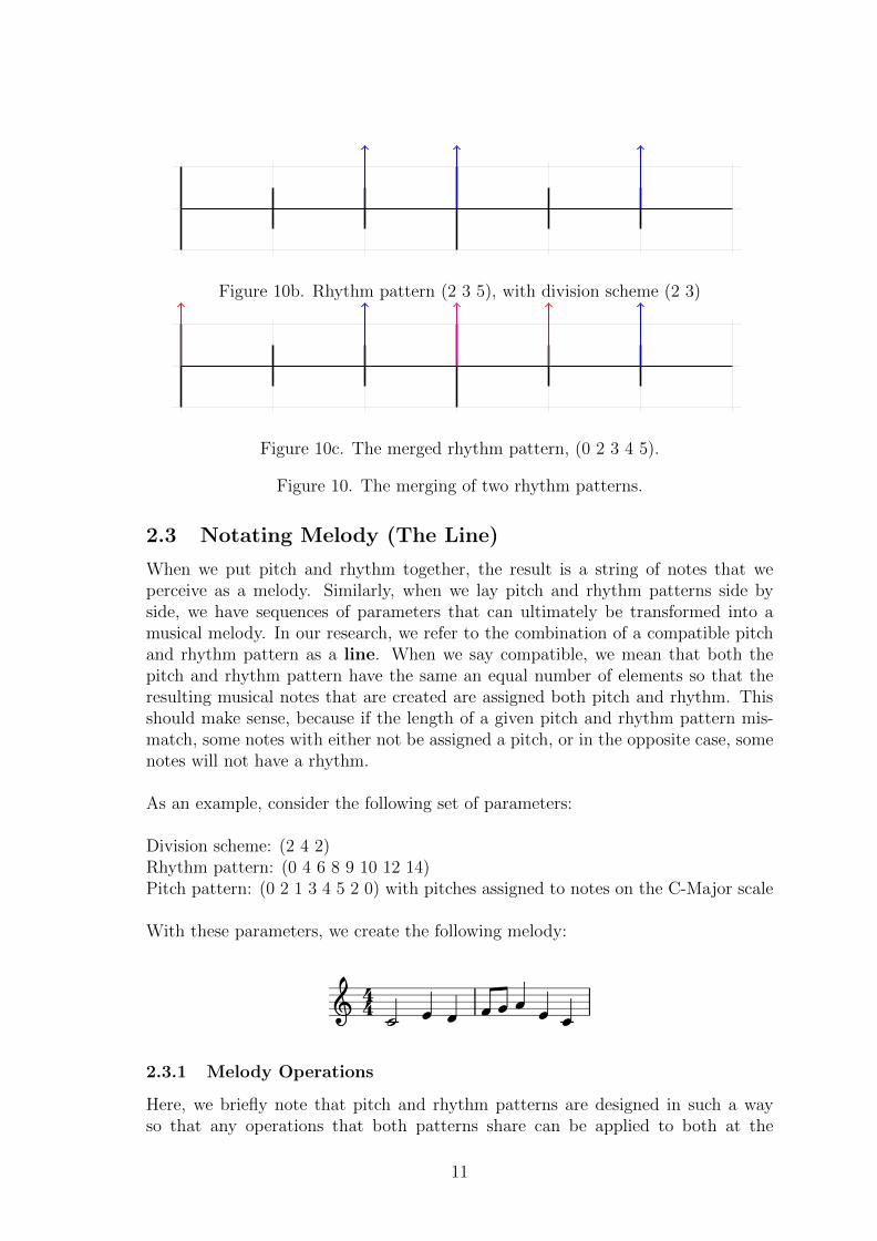
Figure 10b. Rhythm pattern (2 3 5), with division scheme (2 3)

Figure 10c. The merged rhythm pattern, (0 2 3 4 5).

Figure 10. The merging of two rhythm patterns.

2.3 Notating Melody (The Line)

When we put pitch and rhythm together, the result is a string of notes that weperceive as a melody. Similarly, when we lay pitch and rhythm patterns side byside, we have sequences of parameters that can ultimately be transformed into amusical melody. In our research, we refer to the combination of a compatible pitchand rhythm pattern as a line. When we say compatible, we mean that both thepitch and rhythm pattern have the same an equal number of elements so that theresulting musical notes that are created are assigned both pitch and rhythm. Thisshould make sense, because if the length of a given pitch and rhythm pattern mis-match, some notes with either not be assigned a pitch, or in the opposite case, somenotes will not have a rhythm.

As an example, consider the following set of parameters:

Division scheme: (2 4 2)Rhythm pattern: (0 4 6 8 9 10 12 14)Pitch pattern: (0 2 1 3 4 5 2 0) with pitches assigned to notes on the C-Major scale

With these parameters, we create the following melody:

2.3.1 Melody Operations

Here, we briefly note that pitch and rhythm patterns are designed in such a wayso that any operations that both patterns share can be applied to both at the

11

same time without causing any problems. This include the unary operations ofrotation and reversal and the binary operations concatenation and composition.Additionally, we can perform as many operations on pitch as we desire withoutworrying about a potential mismatch in the length of the corresponding rhythmpattern. However, unary rhythm operations that alter the number of events in apattern (e.g. complementation) cannot be applied to a line, because there is nonatural way to assign pitches to the altered rhythms.

2.4 Substitution Schemes

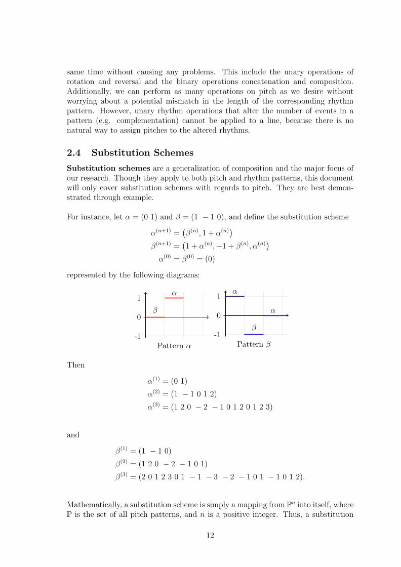
Substitution schemes are a generalization of composition and the major focus ofour research. Though they apply to both pitch and rhythm patterns, this documentwill only cover substitution schemes with regards to pitch. They are best demon-strated through example.

For instance, let ↵ = (0 1) and � = (1 � 1 0), and define the substitution scheme

↵(n+1) =��(n), 1 + ↵(n)

�

�(n+1) =�1 + ↵(n),�1 + �(n),↵(n)

�

↵(0) = �(0) = (0)

represented by the following diagrams:

-1

0

1

�

↵

Pattern ↵

-1

0

1↵

�

↵

Pattern �

Then

↵(1) = (0 1)

↵(2) = (1 � 1 0 1 2)

↵(3) = (1 2 0 � 2 � 1 0 1 2 0 1 2 3)

and

�(1) = (1 � 1 0)

�(2) = (1 2 0 � 2 � 1 0 1)

�(3) = (2 0 1 2 3 0 1 � 1 � 3 � 2 � 1 0 1 � 1 0 1 2).

Mathematically, a substitution scheme is simply a mapping from Pn into itself, whereP is the set of all pitch patterns, and n is a positive integer. Thus, a substitution

12

scheme transforms a vector of n pitch patterns into another vector of n pitch pat-terns. In this research we have focused on substitution schemes that utilize the basicunary and binary pitch operations defined above. By iterating these schemes we cangenerate pitch patterns that exhibit interesting structure, both from a musical anda mathematical point of view.

We will now analyze a couple di↵erent aspects of substitution schemes. We willfirst demonstrate how one can solve for the length of a substitution scheme, andthen we will prove how to solve for any element of a substitution scheme.

2.4.1 Solving for Length

We can use linear algebra techniques to solve for the lengths of the sequences pro-duced by substitution schemes. Specifically, we can create a matrix representing thenumber of pitch patterns involved in each row of a substitution scheme, find theeigenvalues of this matrix, and ultimately use diagonalization (see for instance [4])to solve for the length of a pitch pattern from any iteration of a substitution scheme.

Consider the substitution scheme

↵n+1 = (↵n, 2� �n, �1 + ↵n, �n)

�n+1 = (↵n)

↵0 = (1 3 2 0) �0 = (2 0 1 1).

Then the lengths ai and bi of ↵ and �, respectively, of each iterate i of this substi-tution scheme are

an+1 = 2an + 2bnbn+1 = an

a0 = 4 b0 = 4.

We may represent this system of equations using matrices.

vn+1 =

an+1

bn+1

�=

2 21 0

� anbn

�= Avn,

where v0 =

a0b0

�=

44

�. It follows that

vn = Avn�1

= A2vn�2

= . . .

= Anv0

for k � 1. But A is diagonalizable, with A = PDP�1, where

P =

1 +

p3 1�

p3

1 1

�

13

and

D =

1 +

p3 0

0 1�p3

�.

It follows that An = PDP�1, and we find that

an =2p3

3

⇣(1 +

p3)n+1 � (1�

p3)n+1 � (1 +

p3)n+1(1�

p3) + (1 +

p3)(1�

p3)n+1

⌘,

bn =2p3

3

⇣(1 +

p3)n � (1�

p3)n � (1 +

p3)n(1�

p3) + (1 +

p3)(1�

p3)n

⌘.

Note that the sequence lengths of any substitution schemes of this kind may beanalyzed in this way.

2.4.2 Solving for Elements

We will now discuss methods for solving for specific elements of the pitch patternsgenerated by certain substitution schemes. We begin with perhaps the simplest kindof substitution scheme, iterated composition.

Theorem 2.2. Let ↵ be a pitch pattern with length m � 2, and let n be a positiveinteger. Then for 0 i < mn, we have

↵ni =

m�1X

k=0

↵i(k)

where i(k) is the kth digit in the n-digit base-m expansion of i, including leadingzeroes.

Proof. Let ↵ and � be pitch patterns of length m and n respectively, and let 0 i mn � 1. (This n is not the same as the n in the statement of the theorem.) Iclaim that the ith entry of the composition ↵� is

(↵�)i = ↵q + �r

where q and r are the quotient and remainder when i is divided by n. To see thisfact, note that by the definition of composition,

↵� = (↵0 + �,↵1 + �, ...,↵m�1 + �) .

This composition contains m blocks which consist of copies of � transposed by anamount specified by the entries in ↵. These blocks have length n and are concate-nated together to form ↵� with length mn. Let b be the block number (indexedat zero) that contains the ith entry. Then b = q, where q is the quotient when i isdivided by n. Since this block contains the indices qn to (q+1)n�1, the position ofthe ith entry is given by qn i qn+(n� 1). Let ⇢ = i� qn. Then 0 ⇢ n� 1.Since 0 r n � 1 where r is the remainder when i is divided by n, then by

14

uniqueness, ⇢ = r. Therefore, to find the ith position in the composition ↵�, welocation the qth block and count r units into it. In other words,

(↵�)i = ↵q + �r,

completing the proof of the claim.Now, to prove theorem 1, assume that ↵ has length m � 2. We induct on the

exponent in ↵n. To prove the theorem is true for n = 1, we must show that

↵1i =

0X

k=0

↵i(k).

Clearly the left side equals ↵i. The right hand side equals

0X

k=0

↵i(k) = ↵i(0).

However, i(0) = i since 0 i < m. Therefore, ↵i(0) = ↵i. Now that the base case isestablished, we will move on to the inductive case.

We will assume that the theorem holds for some positive integer n, and consider↵n+1. By claim 0, we have

↵n+1i = (↵n↵)i = ↵n

q + ↵r

where q and r are the quotient and remainder when i is divided by m. Thus,

i = qm+ r

where 0 r < m.

I now claim that r is the lowest-order digit in the base-m expansion of i. Letthe base-m expansion of i be

i = i`m` + i`�1m

`�1 + ...+ i1m+ i0

where 0 ik m� 1 for 0 k `. Then

i = m�i`m

`�1 + i`�1m`�2 + ...+ i1

�+ i0

where i`m`�1 + i`�1m`�2 + ... + i1 is an integer and 0 i0 m � 1. So by theuniqueness of the quotient and remainder, i0 is the remainder when i is divided bym.

In other words, i(n) = r. By the inductive assumption,

↵nq =

n�1X

k=0

↵q(k)

15

where q(k) is the ith digit in the n-digit base-m expansion of q. Then

↵n+1i = ↵n

q + ↵r

= ↵q(0) + ↵q(1) + ...+ ↵q(n�1) + ↵r.

Now we must show that q(k) = i(k) for 0 k n� 1.

To this end, I claim that if

i = (i` i`�1 ... i1 i0)m

and we let i = qm+ r where 0 r m� 1, then

q = (i` i`�1 ... i1)m.

Again,

i = i`m` + i`�1m

`�1 + ...+ i1m+ i0

where 0 ik m� 1 for 0 k `. By the division algorithm, there exists uniqueintegers q and r such that

i = qm+ r

where 0 r m� 1. So

i`m` + i`�1m

`�1 + ...+ i1m+ i0 = qm+ r,

but since 0 r m� 1, i0 = r (by claim 1). So

i`m` + i`�1m

`�1 + ...+ i1m = qm

i`m`�1 + i`�1m

`�2 + ...+ i1 = q

as claimed. By the inductive assumption, ↵nq is the sum of the values of the base-m

digits of q, and therefore ↵n+1i is the sum of the values of the base-m digits of i,

completing the induction and the proof. ⌅We will now discuss two specific cases of substitution schemes: palindromic andrearrangement schemes.

2.4.3 Palindromic Substitution Schemes

We say that a pitch pattern ↵ of length m is palindromic if and only if

↵ = ↵.

In terms of indices,

↵k = ↵m�1�k.

It turns out that if a pitch pattern is palindromic, then its composition with itselfis also palindromic. In order to prove this, we first need two lemmas:

16

Lemma 2.3. To reverse a pitch pattern ↵ composed of n blocks, we reverse the orderof all blocks, then reverse the elements in each individual block.

Proof. (By Induction) (Base) When n = 1, ↵ = (↵0 ↵1 . . . ↵i�1) for an ↵ of lengthi, and following the lemma, the reverse is indeed (↵i�1 ↵i�2 . . . ↵0) = ↵.(Inductive Step) We assume the reverse of ↵ consisting of p blocks is obtainedfollowing the lemma, and we need to show that ↵ of p+1 blocks is reversible by thelemma for all patterns with p blocks. We label each block as ✓i, and each can be apitch pattern of any length. Then for an ↵ of size p+ 1 blocks, we have

↵ = (✓0, ✓1, . . . , ✓p�1, ✓p)

= (�, ✓p)

where � = (✓0, . . . , ✓p�1) has p blocks. By the inductive assumption,

↵ = (�, ✓p)

=�✓p, �

�(Inductive assumption when p = 2)

=�✓p, ✓p�1, . . . , ✓0

�(Inductive assumption when p = n).

⌅Lemma 2.4. For constant k and pitch pattern ↵ of length m, k + ↵ = k + ↵.

Proof. We have

k + ↵ = (k + ↵0, k + ↵1, . . . , k + ↵m�1)

and by lemma 2.3

k + ↵ = (k + ↵m�1, k + ↵m�2, . . . , k + ↵0).

Since k is constant, it follows that its reversal is the same constant, such thatk + ↵ = k + ↵. ⌅And now for our major two claims of this section.

Theorem 2.5. If a pitch pattern ↵ is palindromic, then ↵n is palindromic.

Proof. (By Induction) (Base) When n = 1, ↵n = ↵1 = ↵, which is palindromic.(Inductive Step) We assume ↵p is palindromic for some p, and we need to show that↵p+1 is palindromic for all p. Mathematically, we must show

↵p+1 = ↵p+1.

Then

↵p+1 = (↵0 + ↵p,↵1 + ↵p, . . . ,↵m�1 + ↵p)

= (↵m�1 + ↵p,↵m�2 + ↵p, . . . ,↵0 + ↵p) (By lemma 2.3)

= (↵m�1 + ↵p,↵m�2 + ↵p, . . . ,↵0 + ↵p) (By lemma 2.4)

= (↵m�1 + ↵p,↵m�2 + ↵p, . . . ,↵0 + ↵p) (Since ↵p is palindromic)

= (↵0 + ↵p,↵1 + ↵p, . . . ,↵m�1 + ↵p) (Since ↵ is palindromic)

= ↵p+1.

⌅

17

Theorem 2.6. The substitution scheme

↵(n+1) =�↵0 + �(n),↵1 + ↵(n),↵0 + �(n)

�

�(n+1) =��0 + ↵(n), �1 + �(n), �0 + ↵(n)

�

↵(0) = �(0) = (0)

is palindromic.

Proof. (By Induction) (Base) When n = 0, ↵1 = (↵0 ↵1 ↵0) and �1 = (�0 �1 �0),which are both palindromic.(Inductive Step) We assume ↵p and �p are both palindromic for some p, and weneed to show that ↵p+1 and �p+1 are palindromic for all p. Then

↵p+1 = (↵0 + �(p),↵1 + ↵(p),↵0 + �(p))

=⇣↵0 + �(p),↵1 + ↵(p),↵0 + �(p)

⌘(By lemma 2.3)

=⇣↵0 + �(p),↵1 + ↵(p),↵0 + �(p)

⌘(By lemma 2.4)

=�↵0 + �(p),↵1 + ↵(p),↵0 + �(p)

�(Since ↵p, �p palindromic inductively)

= ↵p+1,

�p+1 = (�0 + ↵(p), �1 + �(p), �0 + ↵(p))

=⇣�0 + ↵(p), �1 + �(p), �0 + ↵(p)

⌘(By lemma 2.3)

=⇣�0 + ↵(p), �1 + �(p), �0 + ↵(p)

⌘(By lemma 2.4)

=��0 + ↵(p), �1 + �(p), �0 + ↵(p)

�(Since ↵p, �p palindromic inductively)

= �p+1.

⌅We now move on to rearrangement schemes.

2.4.4 Rearrangement Schemes

We define a rearrangement scheme as a substitution scheme in which any numberof pitch patterns are merely rearranged in each iteration. We claim the following:

Theorem 2.7. Let b � 2 be an integer. For 0 ` b� 1, the substitution scheme

↵`,n+1 =�↵`,n,↵`+1,n, . . . ,↵`+b�1,n

�(1)

↵`,0 = (`)

where ` is the sequence index and n is the iterate index, is solved by

↵`,nk = (|k|b + `) mod b

for all n, where k is the position index of each substitution scheme.

18

To clearly illustrate the substitution schemes in this theorem, let us give a couple ofexamples. When b = 2,

↵0,n+1 =�↵0,n,↵1,n

�

↵1,n+1 =�↵1,n,↵0,n

�

↵0,0 = (0), ↵1,0 = (1),

and when b = 3,

↵0,n+1 =�↵0,n,↵1,n,↵2,n

�

↵1,n+1 =�↵1,n,↵2,n,↵0,n

�

↵2,n+1 =�↵2,n,↵0,n,↵1,n

�

↵0,0 = (0), ↵1,0 = (1), ↵2,0 = (2),

and so on.To prove this theorem, we first must introduce another lemma:

Lemma 2.8. Let 0 j b�1. Then if j ·bn k (j+1)bn�1, then |k�j ·bn|b =|k|b � j.

Proof. The binary expansion of k has n+ 1 digits,

j bn�1 bn�2 . . . b2 b1 b0,

where the most significant digit is j because j · bn k (j + 1)bn � 1. So

k � j · bn = j bn�1 . . . b1 b0 � j 0n�1 . . . 01 00= 0 bn�1 bn�2 . . . b2 b1 b0.

Therefore, the base-b weight of k � j · bn is j less than the base-b weight of k, and|k � j · bn|b = |k|b � j. ⌅

Now we can prove our theorem.

Proof. (By Induction) (Base) Suppose n = 0. We need to show that

↵`,0k = (|k|b + `) mod b

for k = 0. But by (1), ↵`,0 = (`), so

↵`,00 = ` = (|0|b + `) mod b

since 0 ` b� 1.

19

(Inductive Step) We assume

↵`,pk = (|k|b + `) mod b

for some p � 0 and all 0 k bp � 1. We must show

↵`,p+1k = (|k|b + `) mod b

for all 0 k bp+1 � 1. Let 0 k bp+1 � 1. Then there exists j such that0 j b� 1, and

j · bp k (j + 1)bp � 1.

In other words, j is the index of block of length bp containing k. Then the index of↵`,p+1k in the jth block is k � j · bn, since each block is of length bp. It follows that

↵`,p+1k = ↵`+j,p

k�j·bp

= (|k � j · bp|b + `+ j) mod b (By the inductive assumption)

= (|k|b � j + `+ j) mod b (By lemma 2.8)

= (|k|b + `) mod b.

⌅

3 Synthesizing Compositions

We now talk about our general approach to synthesizing music using the recursivemethods we describe above.

3.1 How to Design Compositions

The foundation for algorithmic musical composition can be approached any numberof ways. Traditionally, we begin by building a substitution scheme that is entirely ar-bitrary and hopefully interesting. We may have an idea of the shape we want a pieceto take, but more often, we just design a substitution scheme that is mathematicallyfascinating, and we let the outcome surprise us. Additionally, while creating oursubstitution schemes, we want to keep in mind which parameters we will utilize. Forexample, we may want a scheme that merely transposes and rearranges our input,or we could create a scheme that additionally rotates and inverts our input.

When considering the operations we have outlined above, we may also decidewhether we want each operation to apply to a motif as a whole, or instead to ourpitch and rhythm patterns independently. For example, we usually rotate a motifby thinking of it as a sequence of notes, but we could by all means rotate pitch andrhythm independently and then reconstruct our motifs afterwards. The arrange-ments of operations in our substitution schemes are only limited by the imaginationof the composer, and these substitution schemes determine the large-scale structureof a composition.

20

After we have outlined the operations we wish to perform, we then design a num-ber of motifs to input into our algorithm. How these motifs are designed ultimatelydetermines the texture of a composition, and through these motifs, we may hear acomposer’s own style emerge. We may also instead choose to mathematically repre-sent a well-known motif, and then mutate said motif with our substitution schemes.For example, we could represent a simplified version of Beethoven’s “Ode to Joy”theme as follows:

Figure 11. The Pitch Pattern ↵ = (2 2 3 4 4 3 2 1 0 0 1 2 2 1 1)

We don’t often design motifs with harmony in mind, because harmony naturallyarises when multiple motifs are played together. When creating motifs, we also tendto create pairs of faster moving parts with higher pitches, and pairs of slower movingparts with lower pitches. Afterwards, we assign a musical instrument to each line inthe output—generally, we assign melodic instruments (like the violin) to higher andquicker parts, and bass instruments (like the electric bass or tuba) lower and slowerparts.

3.2 Tweaking the Music

If we want a piece to be played purely through software, we often don’t make anyfinal tweaks to our music because software can handle any musical oddity thrownat it. However, if we want our music to be played by a musician on a traditionalmusical instrument, we often need to make adjustments to the sheet music to meeta musician’s demands, particularly when it comes to pitch. We could of course justarbitrarily revise sheet music on a whim, but these revisions would ultimately dis-qualify a piece as a pure algorithmic composition. Therefore, we instead present anumber of ways to mathematically tweak music so that the process remains algo-rithmic as well as transparent.

Another aspect of our algorithmic process to consider is that oftentimes, itera-tively generated music ends abruptly. As a result, we may decide to concatenate afinal measure or two of new music onto the end of a composition to give it a greatersense of finality.

3.2.1 Final Transpositions

One of the more obvious problems that occurs after many iterations of a substitutionscheme is that all of the elements in the resulting pitch patterns may be rather smallor large, resulting in very low or high pitches. If we were to assign one of these partsto a musical instrument, we may want to transpose it up or down to meet a player’sneeds, often by utilizing octave equivalence. With multiple instruments playing apiece, if too many instruments are playing in the same frequency range, the piecemay often sound chaotic and muddy, and will often be quite dissonant. We mayreduce this cluttering by transposing lines apart.

21

3.2.2 The Modulo Operation

Another problem that potentially arises after many iterations of a recursively gen-erated pitch pattern is that the di↵erence between the smallest and largest integerscan become quite large. When converted to pitches, extreme values from a pitchpattern in either direction create a variety of problems. In the worst case, a pitchmay be so extreme that it falls outside the range of human hearing, or it may reacha point that is at least not pleasing to listen to. For most musical instruments thatcan only play a limited number of octaves, extreme pitches become unwieldy or evenunplayable. With these problems in mind, we utilize a couple of methods to resolvethese issues in a mathematically satisfying fashion.

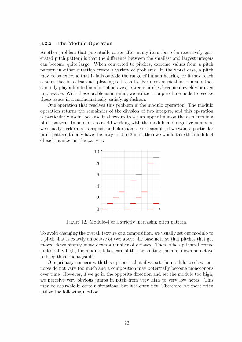
One operation that resolves this problem is the modulo operation. The modulooperation returns the remainder of the division of two integers, and this operationis particularly useful because it allows us to set an upper limit on the elements in apitch pattern. In an e↵ort to avoid working with the modulo and negative numbers,we usually perform a transposition beforehand. For example, if we want a particularpitch pattern to only have the integers 0 to 3 in it, then we would take the modulo-4of each number in the pattern.

0

2

4

6

8

10

Figure 12. Modulo-4 of a strictly increasing pitch pattern.

To avoid changing the overall texture of a composition, we usually set our modulo toa pitch that is exactly an octave or two above the base note so that pitches that getmoved down simply move down a number of octaves. Then, when pitches becomeundesirably high, the modulo takes care of this by shifting them all down an octaveto keep them manageable.

Our primary concern with this option is that if we set the modulo too low, ournotes do not vary too much and a composition may potentially become monotonousover time. However, if we go in the opposite direction and set the modulo too high,we perceive very obvious jumps in pitch from very high to very low notes. Thismay be desirable in certain situations, but it is often not. Therefore, we more oftenutilize the following method.

22

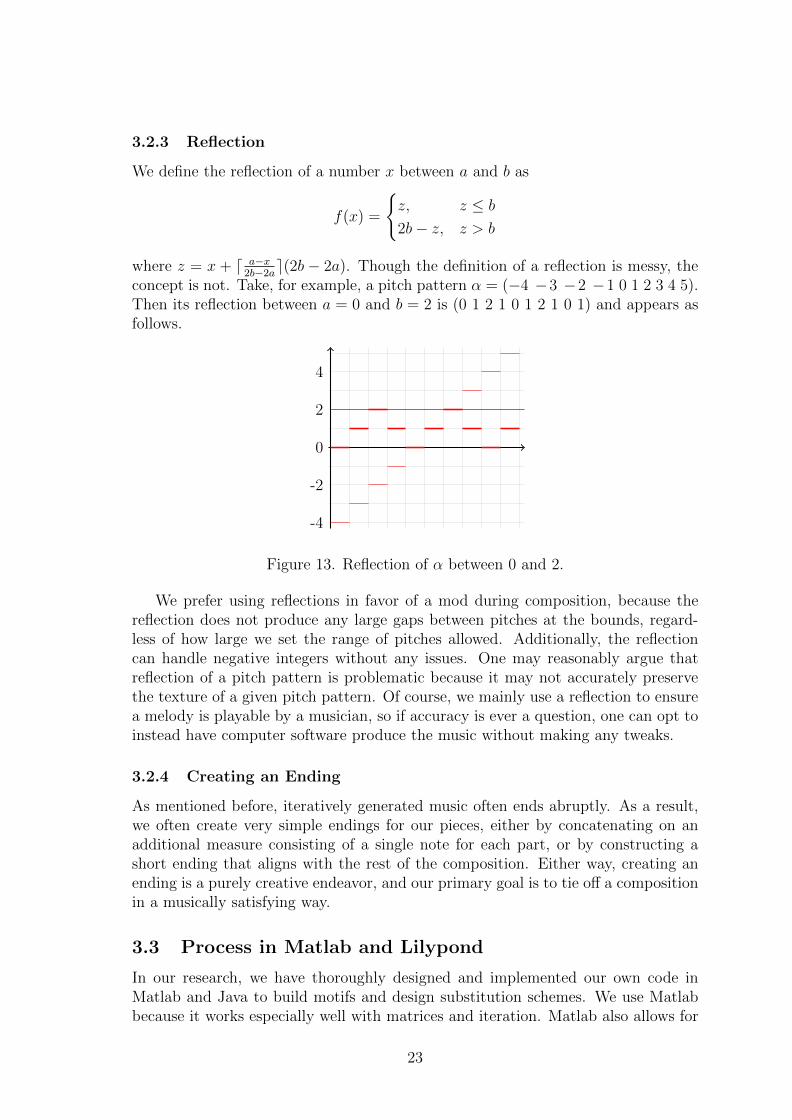
3.2.3 Reflection

We define the reflection of a number x between a and b as

f(x) =

(z, z b

2b� z, z > b

where z = x + d a�x2b�2ae(2b � 2a). Though the definition of a reflection is messy, the

concept is not. Take, for example, a pitch pattern ↵ = (�4 �3 �2 �1 0 1 2 3 4 5).Then its reflection between a = 0 and b = 2 is (0 1 2 1 0 1 2 1 0 1) and appears asfollows.

-4

-2

0

2

4

Figure 13. Reflection of ↵ between 0 and 2.

We prefer using reflections in favor of a mod during composition, because thereflection does not produce any large gaps between pitches at the bounds, regard-less of how large we set the range of pitches allowed. Additionally, the reflectioncan handle negative integers without any issues. One may reasonably argue thatreflection of a pitch pattern is problematic because it may not accurately preservethe texture of a given pitch pattern. Of course, we mainly use a reflection to ensurea melody is playable by a musician, so if accuracy is ever a question, one can opt toinstead have computer software produce the music without making any tweaks.

3.2.4 Creating an Ending

As mentioned before, iteratively generated music often ends abruptly. As a result,we often create very simple endings for our pieces, either by concatenating on anadditional measure consisting of a single note for each part, or by constructing ashort ending that aligns with the rest of the composition. Either way, creating anending is a purely creative endeavor, and our primary goal is to tie o↵ a compositionin a musically satisfying way.

3.3 Process in Matlab and Lilypond

In our research, we have thoroughly designed and implemented our own code inMatlab and Java to build motifs and design substitution schemes. We use Matlabbecause it works especially well with matrices and iteration. Matlab also allows for

23

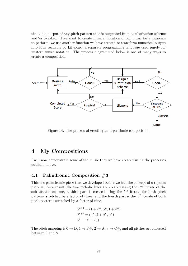
the audio output of any pitch pattern that is outputted from a substitution schemeand/or tweaked. If we want to create musical notation of our music for a musicianto perform, we use another function we have created to transform numerical outputinto code readable by Lilypond, a separate programming language used purely forwestern music notation. The process diagrammed below is one of many ways tocreate a composition.

Figure 14. The process of creating an algorithmic composition.

4 My Compositions

I will now demonstrate some of the music that we have created using the processesoutlined above.

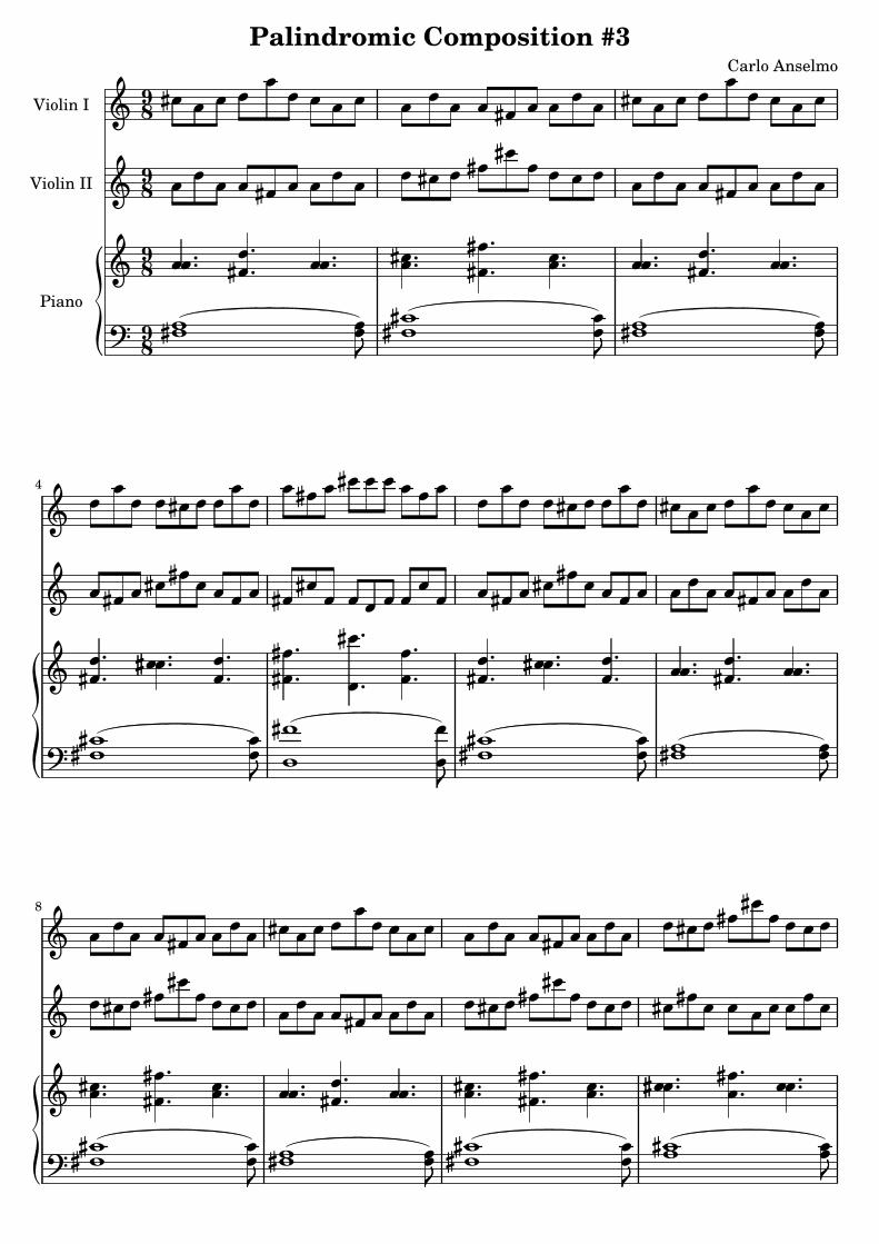
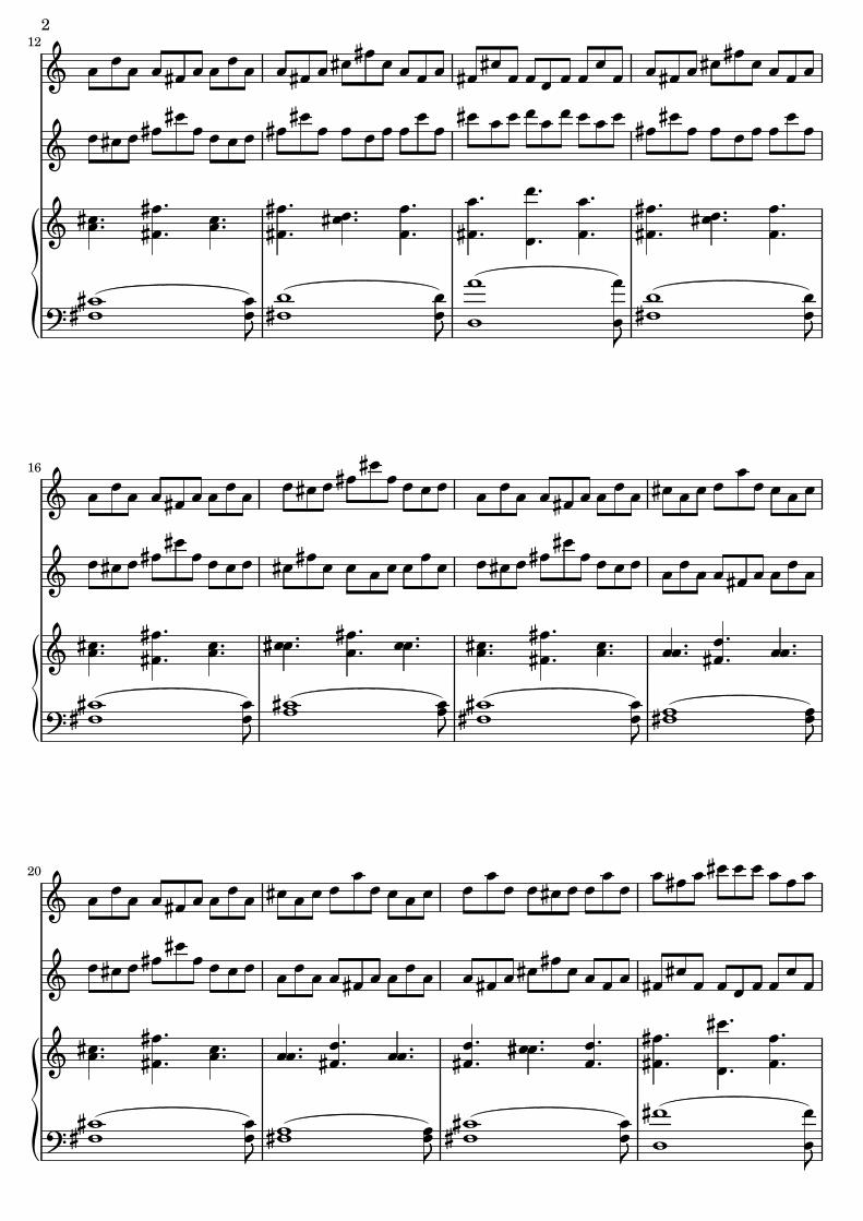
4.1 Palindromic Composition #3

This is a palindromic piece that we developed before we had the concept of a rhythmpattern. As a result, the two melodic lines are created using the 6th iterate of thesubstitution scheme, a third part is created using the 5th iterate for both pitchpatterns stretched by a factor of three, and the fourth part is the 4th iterate of bothpitch patterns stretched by a factor of nine.

↵n+1 = (1 + �n,↵n, 1 + �n)

�n+1 = (↵n, 2 + �n,↵n)

↵0 = �0 = (0)

The pitch mapping is 0 ! D, 1 ! F#, 2 ! A, 3 ! C#, and all pitches are reflectedbetween 0 and 8.

24

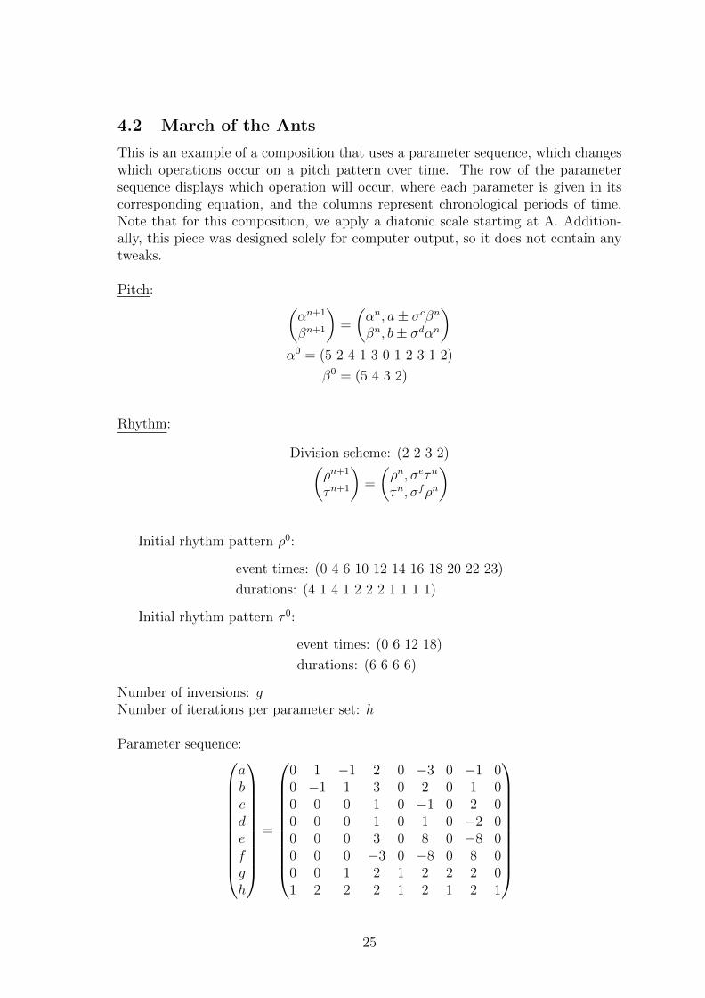
4.2 March of the Ants

This is an example of a composition that uses a parameter sequence, which changeswhich operations occur on a pitch pattern over time. The row of the parametersequence displays which operation will occur, where each parameter is given in itscorresponding equation, and the columns represent chronological periods of time.Note that for this composition, we apply a diatonic scale starting at A. Addition-ally, this piece was designed solely for computer output, so it does not contain anytweaks.

Pitch:✓↵n+1

�n+1

◆=

✓↵n, a± �c�n

�n, b± �d↵n

◆

↵0 = (5 2 4 1 3 0 1 2 3 1 2)

�0 = (5 4 3 2)

Rhythm:

Division scheme: (2 2 3 2)✓⇢n+1

⌧n+1

◆=

✓⇢n, �e⌧n

⌧n, �f⇢n

◆

Initial rhythm pattern ⇢0:

event times: (0 4 6 10 12 14 16 18 20 22 23)

durations: (4 1 4 1 2 2 2 1 1 1 1)

Initial rhythm pattern ⌧ 0:

event times: (0 6 12 18)

durations: (6 6 6 6)

Number of inversions: gNumber of iterations per parameter set: h

Parameter sequence:0

BBBBBBBBBB@

abcdefgh

1

CCCCCCCCCCA

=

0

BBBBBBBBBB@

0 1 �1 2 0 �3 0 �1 00 �1 1 3 0 2 0 1 00 0 0 1 0 �1 0 2 00 0 0 1 0 1 0 �2 00 0 0 3 0 8 0 �8 00 0 0 �3 0 �8 0 8 00 0 1 2 1 2 2 2 01 2 2 2 1 2 1 2 1

1

CCCCCCCCCCA

25

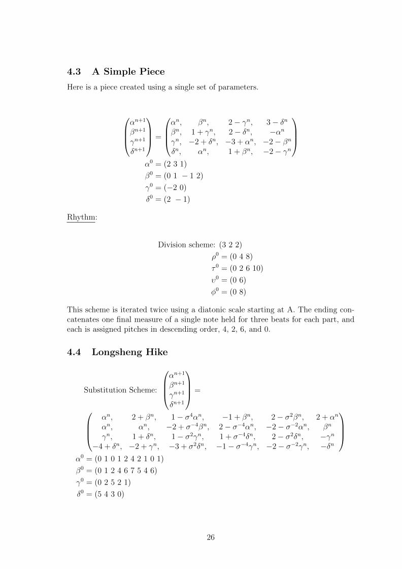
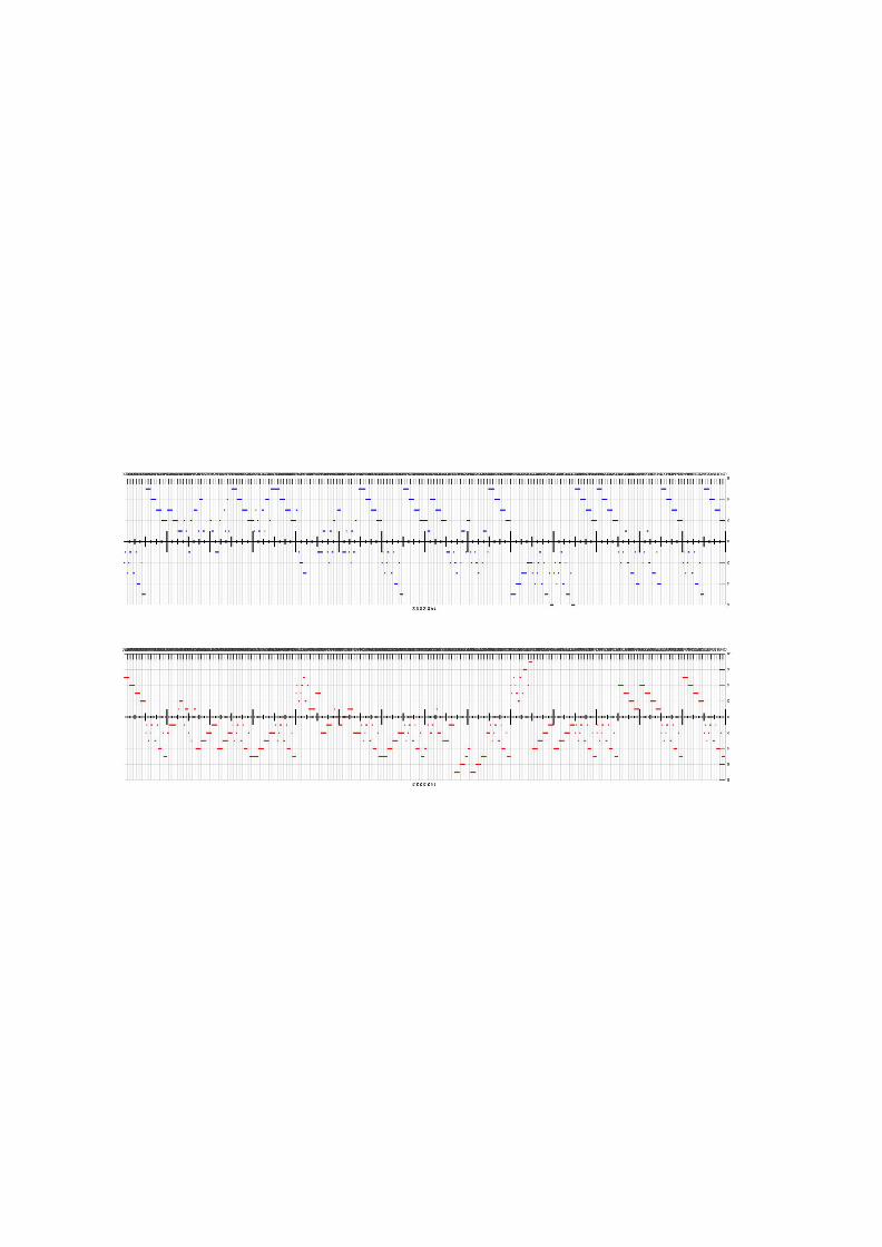
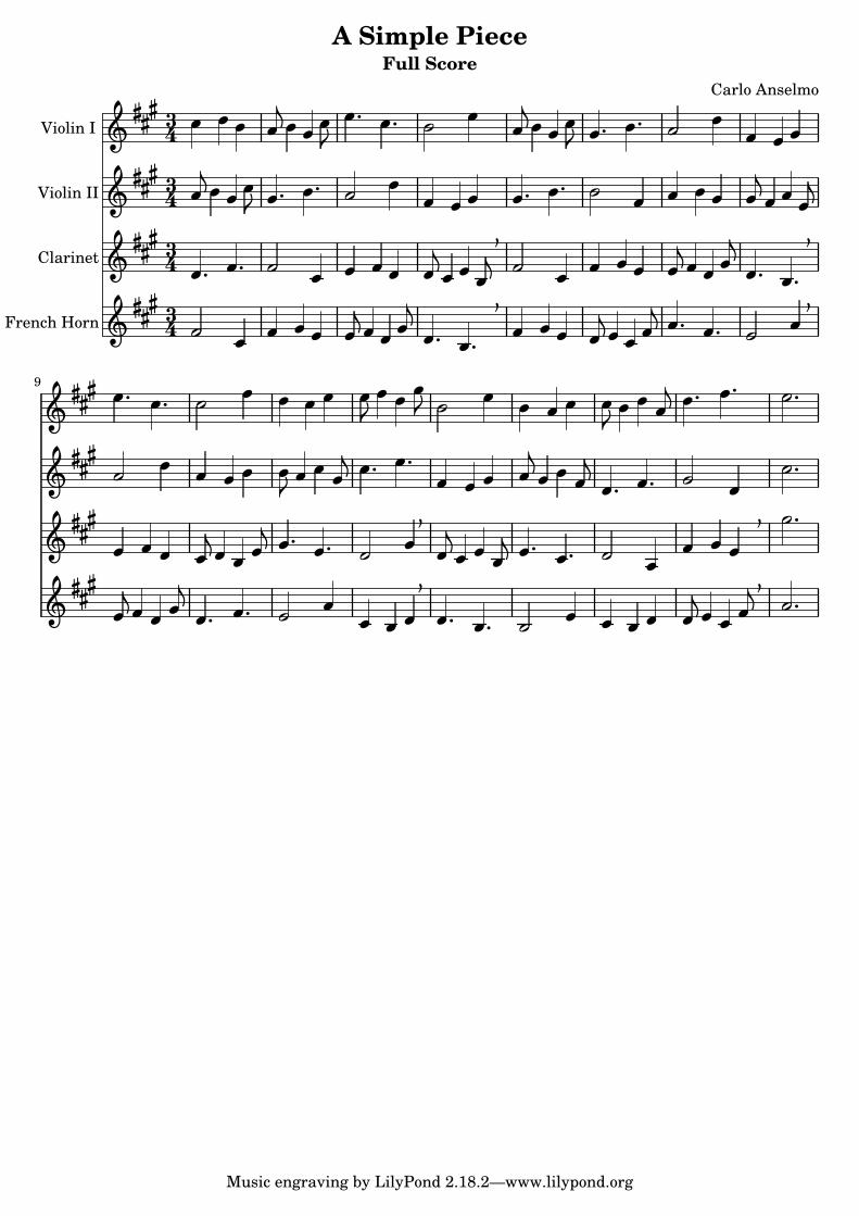
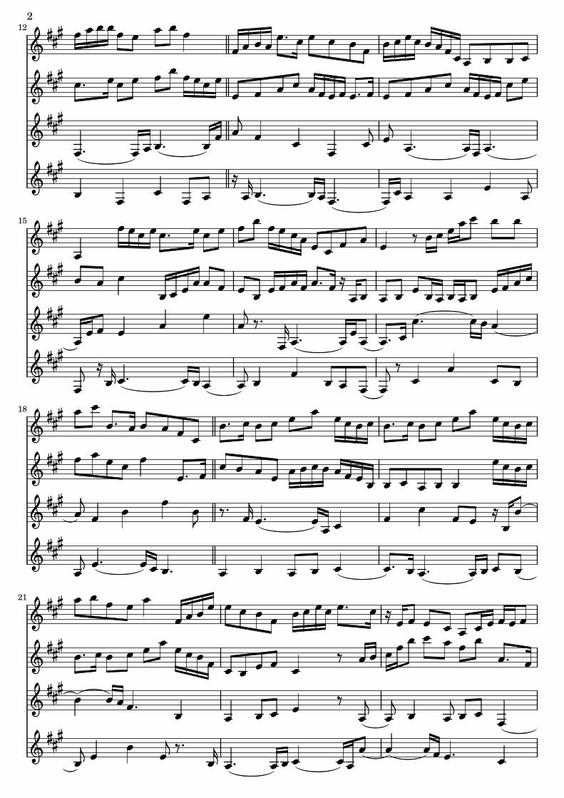
4.3 A Simple Piece

Here is a piece created using a single set of parameters.

0

BB@

↵n+1

�n+1

�n+1

�n+1

1

CCA =

0

BB@

↵n, �n, 2� �n, 3� �n

�n, 1 + �n, 2� �n, �↵n

�n, �2 + �n, �3 + ↵n, �2� �n

�n, ↵n, 1 + �n, �2� �n

1

CCA

↵0 = (2 3 1)

�0 = (0 1 � 1 2)

�0 = (�2 0)

�0 = (2 � 1)

Rhythm:

Division scheme: (3 2 2)

⇢0 = (0 4 8)

⌧ 0 = (0 2 6 10)

�0 = (0 6)

�0 = (0 8)

This scheme is iterated twice using a diatonic scale starting at A. The ending con-catenates one final measure of a single note held for three beats for each part, andeach is assigned pitches in descending order, 4, 2, 6, and 0.

4.4 Longsheng Hike

Substitution Scheme:

0

BB@

↵n+1

�n+1

�n+1

�n+1

1

CCA =

0

BB@

↵n, 2 + �n, 1� �4↵n, �1 + �n, 2� �2�n, 2 + ↵n

↵n, ↵n, �2 + ��4�n, 2� ��4↵n, �2� ��2↵n, �n

�n, 1 + �n, 1� �2�n, 1 + ��4�n, 2� �2�n, ��n

�4 + �n, �2 + �n, �3 + �2�n, �1� ��4�n, �2� ��2�n, ��n

1

CCA

↵0 = (0 1 0 1 2 4 2 1 0 1)

�0 = (0 1 2 4 6 7 5 4 6)

�0 = (0 2 5 2 1)

�0 = (5 4 3 0)

26

Rhythm:

Division scheme: (4 2 2)

⇢0 = (0 3 4 6 8 10 12 13 14 15)

⌧ 0 = (0 1 2 3 4 6 8 10 12)

�0 = (0 4 8 12 14)

�0 = (0 7 8 15)

This scheme is iterated twice using a pentatonic scale starting at A. The first part’spitch pattern is transposed up by two, while the third and fourth part are transposeddown by 7. Finally, the first and second pitch patterns are reflected between -5 and7, the third part is reflected between -11 and -1, and the fourth part is reflectedbetween -11 and 0. After these reflections, the third and fourth parts are transposedup by 5. The ending concatenates one final measure of a single note held for fourbeats for each part, and each is assigned pitches in descending order, -3, 3, 5, and-5.

Additionally, we have altered the staging of the voices slightly: In the first 6measures, the second and fourth instruments don’t play. In measures 31-36, thethird and fourth instruments don’t play.

5 Conclusion

We have reported on several techniques we have developed for generating musicalcompositions algorithmically. We have used sequences of integers called pitch pat-terns and rhythm patterns and their respective operations to generate list of integersthat, through iteration, are increasingly long and complex. The primary tool thatwe have used to iteratively generate these patterns is the substitution scheme, whichtake shorter, simpler pitch and rhythm patterns, and transform them into longer andmore complicated sequences. We have also presented two special cases of substitu-tion schemes. We ultimately use the integers from pitch and rhythm patterns tocreate musical melodies.

When synthesizing new compositions, we design a number of substitution schemesand short motifs, and our process handles the rest of the details. We have also takeninto consideration a musician’s needs for sheet music, and we have designed a numberof methods for performing mathematical tweaks on music to make it more playable.Finally, we present several examples of musical compositions produced by this pro-cess.

Future work includes analyzing existing compositions by popular composers tosee if they even loosely follow our algorithmically techniques. From our minimalexploration of this area, it seems as though musical compositions rarely follow ourprecise methods of generating music, but it is worth noting that at least the shapeof many di↵erent types of music can be expressed using our generative techniques.For example, the majority Prelude in C from The Well Tempered Clavier by J.S.Bach follows a basic (1 2 3 4 5 3 4 5) scheme until the very last few measures.

27

Parts of other pieces, like the introduction Beethoven’s 5th, also follow schemes withdefinitive patterns, in this case following a (0 � 2 � 1 � 3) scheme.

Other topics that we would like to explore would be a deeper mathematical ex-ploration of rhythm patterns and division schemes. We would also like to implementa number of more complicated methods for generating music, such as “triggers” thatalter the music after observing a certain sequence of elements in pitch and rhythmschemes. Finally, we are interested in designing an app that lets the user enter theirown motifs, choose a set of operations, and then listen to the output.

References

[1] T. Johnson, Self-Similar Melodies, Editions 75, 1996.

[2] M. Pendergrass, Patterns and Schemes for Algorithmic Composition, preprint,2016.

[3] M. Pendergrass, Musical Structures and Operations, preprint, 2018.

[4] D. C. Lay, Linear Algebra and Its Application, Addison Wesley, 2003.

28

Appendix I: Palindromic Composition #3

Palindromic Composition #3Carlo Anselmo

!

"

#

$ "

"""

"

" "

"

!

""

"

"

"" !

%

#

!

"

"

""%

""

""

&&

"

""%%

!!##

89 "

"!!#

"

"

!

$

""

"

"

"

"

"" !

#""

89

""

##$

""#

&

"

"

&

""

"""" !!

89

"

"Violin I

Violin II

Piano !##

"

#

!!

#

"

""

"

""

"

89

"

"""

""

"

" #

"

"!!#

"

"

&&

#

%%

"

"

""#

!'

!

!

"

"

"

"

""

"

"""! !!

%%

"

"""&&

"

"

#

# "!!##

#

#!

#

"

"

"

"

"

"""

#

!

"

"

""%

"" !!

"

"

%

"

"

""

&&

#

#

"

"

"

"

""###

"

"

##

"

"

"

"#

!!##

""

"

"

"" !!#

"

"#

"

"

%%

"" ""

"

"

""'

!!"

4

$

$

$

"

""" !!

#

""

"

"

"

""" !!#

""##

"

"

%%

"

"""&&

"

"

"

"

""##

"

"#

"

""""&&

!!#

"

"

""

#

!!#

#

#!!

""

"

"

!!&&""

"

"

%%""

"

"

#" ""

!!""

"

"

"

"

"" "

# !!"""

"

"

""

!!

&

#

##

"

"

" !""

"

"

%%

##""

##!! ""

""

&

""

""

#"

""

"

"

#

""

""

#! # !!

# ##""

#""

""

"

"

&&""

"

"

%%'

"

"

#

8

$

$

$

#"

"""

"

"

" #

"

"

# !!

##

# !!

""

#"

"

""

"

"

&&

""

""

%%

""

##

!!""

""

!

#""

""

""

##!

2

""

##

# !!

#

""

""

!!

# ""

#

##""

"" #

&&

""

""

%%

""#

"

"""

!!""

"""

#"

"

##

# ""

""

"

!!

&&

""

""

"

""

"

"

!!

&&

""

""

%%"

#""

##!!

#

""

""

""

##

%

""

"

#" ""

"

"

"

# !!

%#

##!

""

##""

" !

'

$

$

$12 "

"""

""

!

""

$ !""

""

""

""

!#!!

# ""#

""

%%""

""

!

#

&&

""

""

!!""

""""

""

""##

""##""

""

""%%

"

"

!!

"

"

!

##%

""

""

&&!

""

""

#

!!

"

"#

""

!!

""#

"

"

"

"

""

"

"

""%%

!#

""

""&&

#

! " !!#

"

"

"

"

"

""

##""""

"

#

!!

##

""

""

""%%

" !!

"

"

'

#

""

""

&&!#

16

$

$

$

#

""""

""!#

##

"

"

# "

"

"

"

"

#

!!#

"

"

"

"

""%

"" !!

""

#

""

!

#

!##

"

" "

"

"

""

#

""

#

&&

"

" "

# !!"""

"

! !

#

""

#

!

""

"

"

&&"""

"

%%

"

"

#" ""

!!""

"

"

#"

"

##

# ""

""

""

!!

&

""

""

"

"

!!

&&

""

"

"

%%""

#""

##!!

#

""

""

""

#

!

#

"""

"

"

"

"

"

#!

### !!

# "

"

" #

#

"

"

' &

"

%%

"

20

$

$

$ !"""

"

""

"

"

"

"

!# !!

#

""

"

"

"

"

##""

#"

"

### !

"

"

#

""

"

"

&&"""

"

%%

!"""

"

"

"

!

3

"

#""

"

"

"

"

"

&&""

"

"

%%

!!

#

""

!!"

%%""

"

"

"

"

# !!"" "

"

"

"

"

#

!!

&&"""

"

"

"

#"

"

### !!

""

"""

"

"

"

# "

"

"

"

!!""

"

"

"

#""

## !!

# ""

#$

"

"

"

"

$

&&""

"

"

' %%

!!

#

"

"

" "

"

""%%

#

$

!!"""

"

#"

"

"

#

"

#"

"

""

""

&&

""

""

##

# !! !!""

""

""

""

"

"""

##!!

# ""24

##

Music engraving by LilyPond 2.18.2—www.lilypond.org

Appendix II: March Of The Ants

Appendix III: A Simple Piece

A Simple PieceFull Score

Carlo Anselmo

! "!

#!!! $

"# %%% 43#

%%% !

!

43!&

!!'!

"$

!!

!'

$!

!

!$!!!

! "

!

!

"

'

!

!$ !! $

"!$

'

!!!

!

!

!! "

%%% 43#

!

!!

!

!&!

'

!!

" !! "

!!

!

! $

$!& !'

!!

"

!!

! "

!

!Violin I

Violin II

Clarinet

French Horn

%%%!

43

$

"

!$

!!

( '( !

$

"

'!

!! "

!

!!!

!

!!

!

!

"

"((

!!

!!!$

! $! !

!

!$

'!

!!!

! ""

!& '

!(!

(!

!! "

!

!!!!

! "

$

" $ !!

!

'!!

"

!$

''

( '( '

"!

!

"

!!

&"

!

!

!$!

!'!

"

!!

!$!

!

!

!

!

!

"!

!!$ !

! $

"!

$

'!

!!

%%%

# %%%

""

9

# %%%

# %%%

#

!

'

!!

"

""

!

!

!$!!!

!!

!

!

!'!

&"

!$

!!!'

!

!! "

!

!"&

Music engraving by LilyPond 2.18.2—www.lilypond.org

Appendix IV: Longsheng Hike

Longsheng HikeFull Score

Carlo Anselmo

!

!""" !# !

!$

!%

!

!! !

&$

!

!"""

!

#!$!!

%!

$

!

%

!

""""""

!

#

!

French Horn

Clarinet

Violin II

Violin I

!

#

!

! !!

!

%&!

! !&

!

!

!

'!

!!

(!

!!

&

!

! $)$!

!!

!!!

&$!$)

!

!

! !

!!! !!

&!

!

!#

"""#

"""#

"""#3 !!

&!

!

"""

!

!

!!

(

!!

!

&!

$!

$!

!

!

!

!!

!

&!

! !!!

!

!

!

!

!!

!

!

! &

! !

!

$

!$

&

!

!!

!

!!

!

&

&

!

!

!

!

!! !!

!

!!!

&!

!!

!

!!

!!

!!

!

"""

# """

# """

6 # """

#

!!

!!&

!!

!!

&!!!

!

!

!

!!!

!

!

!!

!

& !

!

!

!

!

(!

!

!

)!

!

!!!

&

!

!

!! !

!

! !!

!

!!

!!

'

!!

!

*!

!

(

!&

!!

+!

!

!

!!

!!

!

&

!

!

&!

!

!!

!

!

!!!

!

!!

!!

&!!

!!

!!

!

!

"""

# """

9 # """

# """

# !!

!!

!))+!

!

! &

!!

!!

&!!

!!

!!

!

!

!

2

(

*!

!

!

!

!

!

!

+!!!

!

!

!!

!

!

!

!

&!

!!! &

!

!!!!

&

!

!!!

!

&

!!

!!

!!

&

!

!

!!

!

!!

!!

!!

!!!

!!

!

! !

&

!

!!!

!

!!!

"""#

"""#

"""#12

!"""# !

!!

!!

(

!

!!(!

!

(

!

!

&!

!

!

&!

!!

&

!!

!

!

!!!!

!

!!

&!

!&!!

!

!

!

!

!

!!

!!

* &

! !

(!!

+!

!

!

!

!

!!

!

!!!! &

!!

!

(

( &

!

)!

!

!

!

!

!!

!

!

)

!

!

!!

!!

!!

!!

*!

!

!

!

!

)

!!

!

&"""#

"""#

"""#15 !

"""# (

!

+!!

!& !

!

!

!

!!

!

!!!

! !

!!

!

!

!

!!

!

!

!!

!

!!

&

!

&

!

!

!!

!

!

!

!!

!

!!

!

!

!

!!

!

!!!

&!

!

! !!

!!!

!

!

!

!

!

!!

!!

!!

!!+

!

! !!

!

&!!

!! &!

!

!

!

!

! &

"""

# """

# """

!!

!

!

18 # """

#

&

!!

(

(

!!

!!

&

!

!!*

!!!!

!

!

!!

!

!

!

!&

! !)

!

&!

,

!!

!!

(! !

!!

!

!!

!

!

!!

!!))

!

& +!

(!!

(

!! !

!

!

!

!

!!

!! &

!!

!

!!

!!

(

!!

!!

!!

&

!!!

!

!!

&

!!

!!

!

!

!*

!

!"""

# """

# """

21 # """

# !

!(!

!!

!)

&

! !!&

!

!!

!

!

! ! !!

!!

!

!

!

!

!!

&

!!!

!

3

&

!

!! !)

!

!

!

!

!$$

!

!

!

!, !

! !

!!

!

& ! ! !

!(!!

!

!

!

!

!

!

!

!

!

!

&

!!

!

!

!!!

! !

!

!

!

!

!

!&

!

# """

# """

# """

24 # """

&

!!

!!

!)+!$

& !- &*

!!

!

!

!

!

!!

!

!!

!

! !

!

!

!$$

!

!(

!

!

!

! !

!

!

!!

! &!

!

$$!

! !! ! !

!

!

!

!! ,

!

! !

!

! !

!

!

!

!

!

!

!"""#

"""#

"""#27

"""

!

#

! ! !

$$!

!)!

!

!+

!

!

!'!

!

!

!

! ! !!

! !

!!

!

!

!

!!!

!

! &

!

!

!!

!!

!

! !

!

!

!!!!

!

!!&

!

! !

!

!

!

!$$

!!!

!

!

! ! !

! !

!

! !"""#

"""#

"""#30

"""#!!

!!

!

!

!

!

!

!

!

!

!

!

!

&

! &!

!

!

!

&

!

!!

!

&!!

&

!

! !!

&

!

!

!

!

!!

' !

!

!

! &

! !!

!

!

!

!

!

!!

!

!

!!

(

+!

!!

&

&

!

&

!

!

!

!

!

!*

!

!

!!

# """"""#

"""#33

!

!

"""#

(!

!!)

!

!

!

!

!!!!

! !

!&

4 ! !

!

!!!

!

!!

&.

.

.

.

!

!!

!! !

!

!

!

! !

!

!)!

+)

!!!

!

!&

&!

&!

!

! !# """

# """

# """

# """

!

!!

35 ! !!

!!

!!

&

!!

!!

! !

!

!!

!

!!

!!!!

!

Music engraving by LilyPond 2.18.2—www.lilypond.org