algorithmic intelligence laboratory (alin-lab) - lec16 network...
TRANSCRIPT

Algorithmic Intelligence Lab
Algorithmic Intelligence Lab
EE807: Recent Advances in Deep Learning
Lecture 16
Slide made by
Jongheon Jeong and Insu Han
KAIST EE
Network Compression

Algorithmic Intelligence Lab
• Deploying deep neural networks (DNNs) has been increasingly difficult• Constraints on power consumption, memory usage, inference overhead, …
• Inference with a large-scale network consumes huge costs
• In mobile apps, such issues become more serious
• “The dreaded 100MB effect”
• Can we make DNNs to perform inferences more efficiently?
Deploying Deep Neural Networks in Real-World
2*source: https://www.recode.net/2016/10/4/13151432/app-size-calculator-bloat-experiment-developers-segment
Algorithmic Intelligence Lab
1. Network Pruning and Re-wiring• Optimal brain damage
• Pruning modern DNNs
• Dense-Sparse-Dense training flow
2. Sparse Network Learning• Structured sparsity learning
• Sparsification via variational dropout
• Variational information bottleneck
3. Weight Quantization• Deep compression
• Binarized neural networks
4. Summary
Table of Contents
3

Algorithmic Intelligence Lab
1. Network Pruning and Re-wiring• Optimal brain damage
• Pruning modern DNNs
• Dense-Sparse-Dense training flow
2. Sparse Network Learning• Structured sparsity learning
• Sparsification via variational dropout
• Variational information bottleneck
3. Weight Quantization• Deep compression
• Binarized neural networks
4. Summary
Table of Contents
4
Algorithmic Intelligence Lab
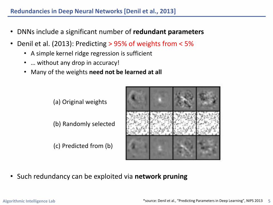
• DNNs include a significant number of redundant parameters
• Denil et al. (2013): Predicting > 95% of weights from < 5% • A simple kernel ridge regression is sufficient
• … without any drop in accuracy!
• Many of the weights need not be learned at all
• Such redundancy can be exploited via network pruning
Redundancies in Deep Neural Networks [Denil et al., 2013]
5*source: Denil et al., “Predicting Parameters in Deep Learning”, NIPS 2013
(a) Original weights
(b) Randomly selected
(c) Predicted from (b)

Algorithmic Intelligence Lab
• Determining low-saliency parameters, given a pre-trained network
• Follows the framework proposed by LeCun et al. (1990):
• Defining which connection is unimportant can vary
• Weight magnitudes (𝐿2, 𝐿1, …)
• Mean activation [Molchanov et al., 2016]
• Avg. % of Zeros (APoZ) [Hu et al., 2016]
• Low entropy activation [Luo et al., 2017]
• …
Network Pruning
6*source: LeCun et al., “Optimal Brain Damage”, NIPS 1990
1. Train a deep model until convergence2. Delete “unimportant” connections w.r.t. a certain criteria3. Re-train the network4. Iterate to step 2, or stop
Algorithmic Intelligence Lab
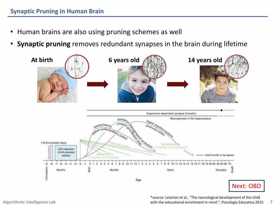
• Human brains are also using pruning schemes as well
• Synaptic pruning removes redundant synapses in the brain during lifetime
Synaptic Pruning in Human Brain
7
At birth 6 years old 14 years old
*source: Leisman et al., “The neurological development of the child with the educational enrichment in mind.”, Psicología Educativa 2015
Next: OBD
Algorithmic Intelligence Lab
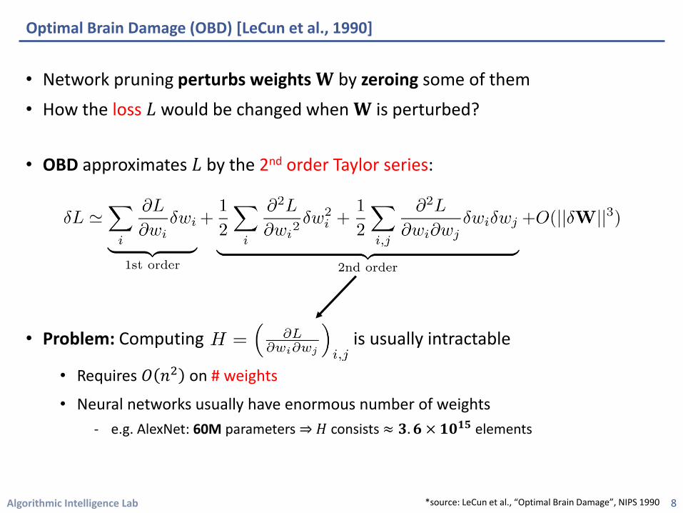
• Network pruning perturbs weights 𝐖 by zeroing some of them
• How the loss 𝐿 would be changed when 𝐖 is perturbed?
• OBD approximates 𝐿 by the 2nd order Taylor series:
• Problem: Computing is usually intractable
• Requires 𝑂 𝑛2 on # weights
• Neural networks usually have enormous number of weights
- e.g. AlexNet: 60M parameters ⇒𝐻 consists ≈ 𝟑. 𝟔 × 𝟏𝟎𝟏𝟓 elements
Optimal Brain Damage (OBD) [LeCun et al., 1990]
8*source: LeCun et al., “Optimal Brain Damage”, NIPS 1990
Algorithmic Intelligence Lab
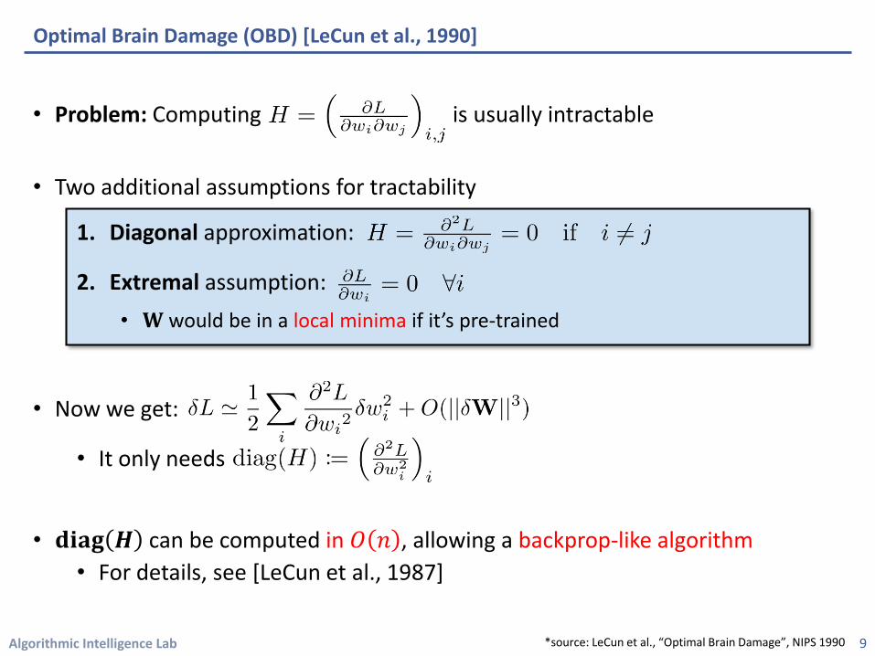
• Problem: Computing is usually intractable
• Two additional assumptions for tractability
1. Diagonal approximation:
2. Extremal assumption:
• 𝐖 would be in a local minima if it’s pre-trained
• Now we get:
• It only needs
• 𝐝𝐢𝐚𝐠 𝑯 can be computed in 𝑂 𝑛 , allowing a backprop-like algorithm
• For details, see [LeCun et al., 1987]
Optimal Brain Damage (OBD) [LeCun et al., 1990]
9*source: LeCun et al., “Optimal Brain Damage”, NIPS 1990

Algorithmic Intelligence Lab
• How the loss 𝐿 would be changed when 𝐖 is perturbed?
• The saliency for each weight ⇒
• OBD shows robustness on pruning compared to magnitude-based deletion
• After re-training, the original test accuracy is recovered
Optimal Brain Damage (OBD) [LeCun et al., 1990]
10*source: LeCun et al., “Optimal Brain Damage”, NIPS 1990
Next: Pruning modern DNNs
w/o re-training
w/ re-training

Algorithmic Intelligence Lab
• Han et al. (2015): Pruning larger DNNs• LeNet, AlexNet, VGG-16, … on ImageNet
• Highlights the practical efficiency of pruning
• OBD introduces extra computation on larger models• It requires an additional, separated backward pass
• The simple magnitude-based pruning works very wellas long as the network is re-trained
Pruning Modern DNNs [Han et al., 2015]
11
Comparison with other model reduction methods on AlexNet
*source: Han et al., “Learning both Weights and Connections for Efficient Neural Networks”, NIPS 2015

Algorithmic Intelligence Lab
• Han et al. (2015): Pruning larger DNNs• Highlights the practical efficiency of pruning
• The magnitude-based pruning works well as long as the network is re-trained
• Network pruning detects visual attention regions
Pruning Modern DNNs [Han et al., 2015]
12
Edge parts of MNIST images
*source: Han et al., “Learning both Weights and Connections for Efficient Neural Networks”, NIPS 2015

Algorithmic Intelligence Lab
• The magnitude-based pruning works well as long as the network is re-trained
• Mittal et al. (2018): In fact, pruning criteria are not that important• … as long as the re-training phase exists
• Many strategies cannot even beat random pruning after fine-tuning
• The compressibility of DNNs are NOT due to the specific criterion • … but due to the inherent plasticity of DNNs
Pruning Modern DNNs
13
Next: Dense-Sparse-Dense
*source: Mittal et al., “Recovering from Random Pruning: On the Plasticity of Deep Convolutional Neural Networks”, WACV 2018

Algorithmic Intelligence Lab
• Network pruning preserves accuracy of the original network
• Han et al. (2017): Re-wiring the pruned connections improves DNNs further• “Dense-Sparse-Dense” training flow
Network Re-wiring: Dense-Sparse-Dense Training Flow
14*source: Han et al., “DSD: Dense-Sparse-Dense Training for Deep Neural Networks”, ICLR 2017

Algorithmic Intelligence Lab
• Network pruning preserves accuracy of the original network
• Han et al. (2017): Re-wiring the pruned connections improves DNNs further• “Dense-Sparse-Dense” training flow
• Pruning discovers better optimum that the current training cannot find
Network Re-wiring: Dense-Sparse-Dense Training Flow
15*source: Han et al., “DSD: Dense-Sparse-Dense Training for Deep Neural Networks”, ICLR 2017

Algorithmic Intelligence Lab
1. Network Pruning and Re-wiring• Optimal brain damage
• Pruning modern DNNs
• Dense-Sparse-Dense training flow
2. Sparse Network Learning• Structured sparsity learning
• Sparsification via variational dropout
• Variational information bottleneck
3. Weight Quantization• Deep compression
• Binarized neural networks
4. Summary
Table of Contents
16
Algorithmic Intelligence Lab
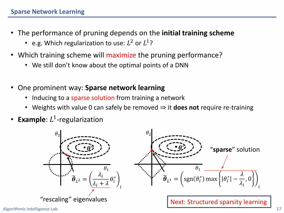
• The performance of pruning depends on the initial training scheme
• e.g. Which regularization to use: 𝐿2 or 𝐿1?
• Which training scheme will maximize the pruning performance?• We still don’t know about the optimal points of a DNN
• One prominent way: Sparse network learning• Inducing to a sparse solution from training a network
• Weights with value 0 can safely be removed ⇒ it does not require re-training
• Example: 𝐿1-regularization
Sparse Network Learning
17
𝜽∗
𝜃1
𝜃2
෩𝜽𝐿2 =𝜆𝑖
𝜆𝑖 + 𝜆𝜃𝑖∗
𝑖
𝜽∗
𝜃1
𝜃2
෩𝜽𝐿1 = sgn 𝜃𝑖∗ max 𝜃𝑖
∗ −𝜆
𝜆𝑖, 0
𝑖
“sparse” solution
“rescaling” eigenvalues Next: Structured sparsity learning

Algorithmic Intelligence Lab
• “Un-structured” weight-level pruning may not engage a practical speed-up• Despite of extremely high sparsity, actual speed-ups in GPU is limited
Structured Sparsity Learning [Wen et al., 2016]
18
Speed-up ratio of weight-level pruning
*source: Wen et al., “Learning structured sparsity in deep neural networks.” NIPS 2016
Algorithmic Intelligence Lab
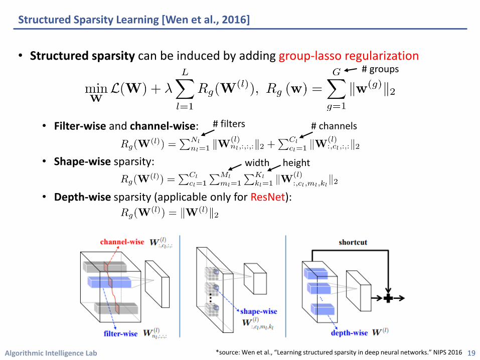
• Structured sparsity can be induced by adding group-lasso regularization
• Filter-wise and channel-wise:
• Shape-wise sparsity:
• Depth-wise sparsity (applicable only for ResNet):
Structured Sparsity Learning [Wen et al., 2016]
19*source: Wen et al., “Learning structured sparsity in deep neural networks.” NIPS 2016
# filters # channels
# groups
width height

Algorithmic Intelligence Lab
• Structured sparsity can be induced by adding group-lasso regularization
• Filter-wise and channel-wise:
Structured Sparsity Learning [Wen et al., 2016]
20*source: Wen et al., “Learning structured sparsity in deep neural networks.” NIPS 2016
# filters # channels

Algorithmic Intelligence Lab
• Structured sparsity can be induced by adding group-lasso regularization
• Shape-wise sparsity:
Structured Sparsity Learning [Wen et al., 2016]
21*source: Wen et al., “Learning structured sparsity in deep neural networks.” NIPS 2016
width height

Algorithmic Intelligence Lab
• Structured sparsity can be induced by adding group-lasso regularization
• Depth-wise sparsity:
Structured Sparsity Learning [Wen et al., 2016]
22
Next: Sparsification via variational dropout
*source: Wen et al., “Learning structured sparsity in deep neural networks.” NIPS 2016

Algorithmic Intelligence Lab
• Variational dropout (VD) allows to learn the dropout rates separately
• Unlike dropout, VD imposes noises on weights 𝜽:
• A Bayesian generalization of Gaussian dropout [Srivastava et al., 2014]
• is adapted to data in Bayesian sense by optimizing 𝛂 and 𝜽
• Re-parametrization trick allows 𝐰 to be learned via minibatch-based gradient estimation methods [Kingma & Welling, 2013]
• 𝛂 and 𝜽 can be optimized separated from noises
Recall: Variational Dropout [Kingma et al., 2015]
23*source : Kingma et al., “Variational dropout and the local reparametrization trick”, NIPS 2015

Algorithmic Intelligence Lab
• VD imposes noises on weights 𝜃:
• The original VD set a constraint for technical reasons
• It corresponds to in binary dropout
Q. What if ? What happens when ?
•
• will be completely random as
• Such will corrupt the expected log likelihood
• … except that as well!
Variational Dropout Sparsifies DNNs [Molchanov et al., 2017]
24*source : Molchanov et al., “Variational Dropout Sparsifies Deep Neural Networks”, ICML 2017

Algorithmic Intelligence Lab
CN
N f
ilter
s
Fully
co
nn
ect
ed la
yer
Q. What if ? What happens when ?
• It will corrupt the expected log likelihood except that as well
• Molchanov et al. (2017): Extending VD for ⇒ Super sparse solutions• Weights with are pruned away during training
Variational Dropout Sparsifies DNNs [Molchanov et al., 2017]
25*source : Molchanov et al., “Variational Dropout Sparsifies Deep Neural Networks”, ICML 2017

Algorithmic Intelligence Lab
Q. What if ? What happens when ?
• It will corrupt the expected log likelihood except that as well
• Molchanov et al. (2017): Extending VD for ⇒ Super sparse solutions• Weights with are pruned away during training
Variational Dropout Sparsifies DNNs [Molchanov et al., 2017]
26
Next: Variational information bottleneck
[Han et al., 2015]
[Han et al., 2015]
*source : Molchanov et al., “Variational Dropout Sparsifies Deep Neural Networks”, ICML 2017

Algorithmic Intelligence Lab
• Motivation: Markov chain interpretation of DNN [Tishby & Zaslavsky, 2015]
1. Maximize 𝐼(𝒉𝑖; 𝒚) for high-accuracy prediction
2. Minimize 𝐼(𝒉𝑖; 𝒉𝑖−1) for compression ⇒ “information bottleneck”
• Layer-wise losses become:
Variational Information Bottleneck [Dai et al., 2018]
27
The relative strength of bottleneck
Approximatevia tractable
Mutual information
*source : Dai et al., “Compressing Neural Networks using the Variational Information Bottleneck”, ICML 2018

Algorithmic Intelligence Lab
• Layer-wise losses become
• Problem: Computing is usually intractable
• Instead, we minimize variational upper bound of it
• Variational Information Bottleneck (VIB) model
Variational Information Bottleneck [Dai et al., 2018]
28
variational approx. of 𝑝(𝒉𝑖) variational approx. of 𝑝(𝒚|𝒉𝐿)
ቊ𝐦𝐮𝐥𝐭𝐢𝐧𝐨𝐦𝐚𝐥𝐆𝐚𝐮𝐬𝐬𝐢𝐚𝐧
for classificationfor regression
ቄReparametrization trick [Kingma & Welling, 2013]
*source : Dai et al., “Compressing Neural Networks using the Variational Information Bottleneck”, ICML 2018

Algorithmic Intelligence Lab
• We minimize variational upper bound of
• Final variational objective function (VIBNet):
• Pruning criteria:
• Neurons with low value of ’s are pruned after training
Variational Information Bottleneck [Dai et al., 2018]
29
ቄReparametrization trick [Kingma & Welling, 2013]
# layers
*source : Dai et al., “Compressing Neural Networks using the Variational Information Bottleneck”, ICML 2018

Algorithmic Intelligence Lab
• VIBNet outperforms various methods by large margins
• 𝑟𝑊(%): ratio of # parameters
• 𝑟𝑁(%): ratio of memory footprint
Variational Information Bottleneck [Dai et al., 2018]
30
Epoch Epoch
*source : Dai et al., “Compressing Neural Networks using the Variational Information Bottleneck”, ICML 2018
After fine-tuning
Algorithmic Intelligence Lab
1. Network Pruning and Re-wiring• Optimal brain damage
• Pruning modern DNNs
• Dense-Sparse-Dense training flow
2. Sparse Network Learning• Structured sparsity learning
• Sparsification via variational dropout
• Variational information bottleneck
3. Weight Quantization• Deep compression
• Binarized neural networks
4. Summary
Table of Contents
31

Algorithmic Intelligence Lab
• Quantizing weights can further compress the pruned networks• Weights are clustered into discrete values
• The network is represented only with several centroid values
• Han et al. (2015): Pruning DNNs ⇒ 9x-13x reduction
• Han et al. (2016): Pruning + Quantization + Huffman ⇒ 35x-49x reduction
Deep Compression [Han et al., 2016]
32
Network Pruning
Weight Quantization
HuffmanEncoding
*source : Han et al., “Deep Compression - Compressing Deep Neural Networks with Pruning, Trained Quantization and Huffman Coding”, ICLR 2016

Algorithmic Intelligence Lab
• Quantizing weights can further compress the pruned networks• Weights are clustered into discrete values
• The network is represented only with several centroid values
• In the fine-tuning phase, gradientsin each cluster are aggregated:
Deep Compression [Han et al., 2016]
33
1. Train a deep model until convergence2. Find 𝑘 clusters that minimizes within-cluster sum of squares (WCSS):
3. Quantize with the cluster via weight sharing 4. Fine-tune the network with the shared weights
*source : Han et al., “Deep Compression - Compressing Deep Neural Networks with Pruning, Trained Quantization and Huffman Coding”, ICLR 2016

Algorithmic Intelligence Lab
Network Original Size Compressed
Size
Compression
Ratio
Original
Accuracy (%)
Compressed
Accuracy (%)
Deep Compression [Han et al., 2016]
34
LeNet-300 1070KB 27KB 40x 98.36 98.42
LeNet-5 1720KB 44KB 39x 99.20 99.26
AlexNet 240MB 6.9MB 35x 80.27 80.30
VGGNet 550MB 11.3MB 49x 88.68 89.09
GoogLeNet 28MB 2.8MB 10x 88.90 88.92
SqueezeNet 4.8MB 0.47MB 10x 80.32 80.35
• Deep compression reduces the model size significantly
*source : Han et al., “Deep Compression - Compressing Deep Neural Networks with Pruning, Trained Quantization and Huffman Coding”, ICLR 2016
Next: Binarized neural networks

Algorithmic Intelligence Lab
Binarized Neural Networks [Hubara et al., 2016]
35
• Neural networks can be even binarized (+1 or -1)• DNNs trained to use binary weights and binary activations
• Expensive 32-bit MAC (Multiply-ACcumulate) ⇒ Cheap 1-bit XNOR-Count• “MAC == XNOR-Count”: when the weights and activations are ±1
+1
+1
+1
+1
+1−1
−1
−1
−1
−1
−1
−1
*source : Hubara et al., “Binarized Neural Networks ”, NIPS 2016
# 1s in bits

Algorithmic Intelligence Lab
Binarized Neural Networks [Hubara et al., 2016]
36
• Idea: Training real-valued nets (𝑊𝑟) treating binarization (𝑊𝑏) as noise• Training 𝑊𝑟 is done by stochastic gradient descent
• Binarization (𝑊𝑟 → 𝑊𝑏) occurs for each forward propagation• On each of weights:
• … also on each activation:
• Gradients for 𝑊𝑟 is estimated from [Bengio et al., 2013]• “Straight-through estimator”: Ignore the binarization during backward!
• Cancelling gradients for better performance
• When the value is too large
+1
+1
+1
+1
+1−1
−1
−1
−1
−1
−1
−1
*source : Hubara et al., “Binarized Neural Networks ”, NIPS 2016

Algorithmic Intelligence Lab
Binarized Neural Networks [Hubara et al., 2016]
37
• Neural networks can be even binarized (+1 or -1)• DNNs trained to use binary weights and binary activations
• BNN yields 32x less memory compared to the baseline 32-bit DNNs
• … also expected to reduce energy consumption drastically
• 23x faster on kernel execution times• BNN allows us to use XNOR kernels
• 3.4x faster than cuBLAS
*source : Hubara et al., “Binarized Neural Networks ”, NIPS 2016

Algorithmic Intelligence Lab
Binarized Neural Networks [Hubara et al., 2016]
38
• Neural networks can be even binarized (+1 or -1)• DNNs trained to use binary weights and binary activations
• BNN achieves comparable error rates over existing DNNs
*source : Hubara et al., “Binarized Neural Networks ”, NIPS 2016

Algorithmic Intelligence Lab
1. Network Pruning and Re-wiring• Optimal brain damage
• Pruning modern DNNs
• Dense-Sparse-Dense training flow
2. Sparse Network Learning• Structured sparsity learning
• Sparsification via variational dropout
• Variational information bottleneck
3. Weight Quantization• Deep compression
• Binarized neural networks
4. Summary
Table of Contents
39

Algorithmic Intelligence Lab
• Broad economic viability requires energy efficient AI [Welling, 2018]• “Energy efficiency of a brain is 100x better than current hardware”
• “AI algorithms will be measured by the amount of intelligence per kWh”
• Network pruning and re-wiring• A simple but effective way to compress DNNs
• Allow us to find better optimum that the current training cannot
• Sparse network learning• Which training scheme will maximize the pruning performance?
• It has gained significant attention recently
• Various other techniques have been also proposed• Weight quantization
• Anytime/adaptive networks [Huang et al., 2018]
• …
Summary
40

Algorithmic Intelligence Lab
References
41
• [LeCun, 1987] Lecun, Y. (1987). PhD thesis: Modeles connexionnistes de l'apprentissage (connectionist learning models).Link: https://nyuscholars.nyu.edu/en/publications/phd-thesis-modeles-connexionnistes-de-lapprentissage-connectionis
• [LeCun et al., 1990] LeCun, Y., Denker, J. S., & Solla, S. A. (1990). Optimal brain damage. In Advances in neural information processing systems (pp. 598-605).Link: http://papers.nips.cc/paper/250-optimal-brain-damage.pdf
• [Bengio et al., 2013] Bengio, Y., Léonard, N., & Courville, A. (2013). Estimating or propagating gradients through stochastic neurons for conditional computation. arXiv preprint arXiv:1308.3432.Link: https://arxiv.org/abs/1308.3432
• [Denil et al., 2013] Denil, M., Shakibi, B., Dinh, L., & De Freitas, N. (2013). Predicting parameters in deep learning. In Advances in neural information processing systems (pp. 2148-2156).Link: http://papers.nips.cc/paper/5025-predicting-parameters-in-deep-learning
• [Kingma & Welling, 2013] Kingma, D. P., & Welling, M. (2013). Auto-encoding variational bayes. arXiv preprint arXiv:1312.6114.Link: https://arxiv.org/abs/1312.6114
• [Han et al., 2015] Han, S., Pool, J., Tran, J., & Dally, W. (2015). Learning both weights and connections for efficient neural network. In Advances in neural information processing systems (pp. 1135-1143).Link: http://papers.nips.cc/paper/5784-learning-both-weights-and-connections-for-efficient-neural-network
• [Kingma et al., 2015] Kingma, D. P., Salimans, T., & Welling, M. (2015). Variational dropout and the local reparameterization trick. In Advances in Neural Information Processing Systems (pp. 2575-2583).Link: http://papers.nips.cc/paper/5666-variational-dropout-and-the-local-reparameterization-trick

Algorithmic Intelligence Lab
References
42
• [Leisman et al., 2015] Leisman, G., Mualem, R., & Mughrabi, S. K. (2015). The neurological development of the child with the educational enrichment in mind. Psicología Educativa, 21(2), 79-96.Link: https://www.sciencedirect.com/science/article/pii/S1135755X15000226
• [Tishby & Zaslavsky, 2015] Tishby, N., & Zaslavsky, N. (2015, April). Deep learning and the information bottleneck principle. In Information Theory Workshop (ITW), 2015 IEEE (pp. 1-5). IEEE.Link: https://ieeexplore.ieee.org/abstract/document/7133169
• [Han et al., 2016] Han, S., Mao, H., & Dally, W. J. (2016). Deep compression: Compressing deep neural networks with pruning, trained quantization and huffman coding. In International Conference on Learning Representations. Link: https://arxiv.org/abs/1510.00149
• [Hu et al., 2016] Hu, H., Peng, R., Tai, Y. W., & Tang, C. K. (2016). Network trimming: A data-driven neuron pruning approach towards efficient deep architectures. arXiv preprint arXiv:1607.03250.Link: https://arxiv.org/abs/1607.03250
• [Hubara et al., 2016] Hubara, I., Courbariaux, M., Soudry, D., El-Yaniv, R., & Bengio, Y. (2016). Binarized neural networks. In Advances in neural information processing systems (pp. 4107-4115).Link: http://papers.nips.cc/paper/6573-binarized-neural-networks
• [Molchanov et al., 2016] Molchanov, P., Tyree, S., Karras, T., Aila, T., & Kautz, J. (2016). Pruning convolutional neural networks for resource efficient inference. arXiv preprint arXiv:1611.06440.Link: https://arxiv.org/abs/1611.06440
• [Wen et al., 2016] Wen, W., Wu, C., Wang, Y., Chen, Y., & Li, H. (2016). Learning structured sparsity in deep neural networks. In Advances in Neural Information Processing Systems (pp. 2074-2082).Link: http://papers.nips.cc/paper/6503-learning-structured-sparsity-in-deep-neural-networks
• [Han et al., 2017] Han, S., Pool, J., Narang, S., Mao, H., Gong, E., Tang, S., ... & Catanzaro, B. (2017). Dsd: Dense-sparse-dense training for deep neural networks. In International Conference on Learning Representations. Link: https://openreview.net/forum?id=HyoST_9xl

Algorithmic Intelligence Lab
References
43
• [Luo et al., 2017] Luo, J. H., Wu, J., & Lin, W. (2017). ThiNet: A Filter Level Pruning Method for Deep Neural Network Compression. In Proceedings of the IEEE International Conference on Computer Vision (pp. 5058-5066).Link: http://openaccess.thecvf.com/content_iccv_2017/html/Luo_ThiNet_A_Filter_ICCV_2017_paper.html
• [Molchanov et al., 2017] Molchanov, D., Ashukha, A. & Vetrov, D.. (2017). Variational Dropout Sparsifies Deep Neural Networks. Proceedings of the 34th International Conference on Machine Learning, in PMLR 70:2498-2507Link: http://proceedings.mlr.press/v70/molchanov17a.html
• [Dai et al., 2018] Dai, B., Zhu, C., Guo, B. & Wipf, D.. (2018). Compressing Neural Networks using the VariationalInformation Bottleneck. Proceedings of the 35th International Conference on Machine Learning, in PMLR 80:1135-1144Link: http://proceedings.mlr.press/v80/dai18d.html
• [Huang et al., 2018] Huang, G., Chen, D., Li, T., Wu, F., van der Maaten, L., & Weinberger, K. Q. (2018). Multi-scale dense networks for resource efficient image classification. In International Conference on Learning Representations Link: https://openreview.net/forum?id=Hk2aImxAb
• [Mittal et al., 2018] Mittal, D., Bhardwaj, S., Khapra, M. M., & Ravindran, B. (2018, March). Recovering from Random Pruning: On the Plasticity of Deep Convolutional Neural Networks. In 2018 IEEE Winter Conference on Applications of Computer Vision (WACV) (pp. 848-857). IEEE.Link: https://www.computer.org/csdl/proceedings/wacv/2018/4886/00/488601a848-abs.html
• [Welling, 2018] Welling, M. (2018). Intelligence per Kilowatthour. Link: https://icml.cc/Conferences/2018/Schedule?showEvent=1866