algorithmic number theory in function fields€¦ · algorithmic number theory in function fields...

Algorithmic Number Theory in FunctionFields

Renate Scheidler

UNCG Summer School in Computational Number Theory 2016:Function Fields

May 30 – June 3, 2016

References

Henning Stichtenoth, Algebraic Function Fields and Codes, seconded., GTM vol. 54, Springer 2009

Michael Rosen, Number Theory in Function Fields, GTM vol. 210,Springer 2002

Gabriel Daniel Villa Salvador, Topics in the Theory of AlgebraicFunction Fields, Birkhauser 2006

Renate Scheidler (Calgary) Number Theory in Function Fields UNGC, Summer 2016 2 / 92

Valuation Theory

Absolute ValuesThroughout, let F be a field.

Definition

An absolute value on F is a map ∣ ⋅ ∣ ∶ F → R such that for all a,b ∈ F :

∣a∣ ≥ 0, with equality if and only if a = 0

∣ab∣ = ∣a∣∣b∣∣a + b∣ ≤ ∣a∣ + ∣b∣ (archimedian) or

∣a + b∣ ≤ max{∣a∣, ∣b∣} (non-archimedian)

Examples

The well-known absolute value on Q (or on R or on C) is anarchimedian absolute value in the sense of the above definition.

The trivial absolute value on any field F , defined via ∣a∣ = 0 whena = 0 and ∣a∣ = 1 otherwise, is a non-archimedian absolute value.


p-Adic Absolute Values on Q

Let p be ay prime number, and define a map ∣ ⋅ ∣p on Q as follows:

For r ∈ Q∗, write r = pna

bwith n ∈ Z and p ∤ ab and set

∣r ∣p = p−n.

Then ∣ ⋅ ∣p is a non-archimedian absolute value on Q, called the p-adicabsolute value on Q.

Theorem (Ostrowski)

The p-adic absolute values, along with the trivial and the ordinary absolutevalue, are the only valuations on Q.


Rational Function Fields

Notation

For any field K :

K [x] denotes the ring of polynomials in x with coefficients in K .

K(x) denotes the field of rational functions in x with coefficients in K :

K(x) = { f (x)g(x) ∣ f (x),g(x) ∈ K [x] with g(x) ≠ 0}.

Note that F = K(x) is our first example of an algebraic function field.More formally:

Definition

A rational function field F /K is a field F of the form F = K(x) wherex ∈ F is transcendental over K .


Absolute Values on K(x)Fix a constant c ∈ R, c > 1, and let r(x) ∈ K(x) be nonzero.

p-adic absolute values on K(x):Let p(x) be any monic irreducible polynomial in K [x], and writer(x) = p(x)na(x)/b(x) with n ∈ Z and p(x) ∤ a(x)b(x). Define

∣r(x)∣p(x) = c−n.

Then ∣ ⋅ ∣p(x) is a non-archimedian absolute value on K(x).

Infinite absolute value on K(x):Write r(x) = f (x)/g(x) and define

∣r(x)∣∞ = cdeg(f )−deg(g).

Then ∣ ⋅ ∣∞ is a non-archimedian absolute value on K(x).


Remarks on Absolute Values on K(x)

These, plus the trivial absolute value, are essentially all the absolutevalues on K(x), up to trivial modifications such as

▸ using a different constant c ,

▸ using a different normalization on the irreducible polynomialsp(x).

All absolute values on K(x) are non-archimedian (different from Q!)

When K = Fq is a finite field of order q, one usually chooses c = q.

When K is a field of characteristic 0, one usually choosesc = e = 2.71828 . . ..


Valuations

Definition

A valuation on F is a map v ∶ F → R ∪ {∞} such that for all a,b ∈ F :

v(a) =∞ if and only if a = 0v(ab) = v(a) + v(b)v(a + b) ≥ min{v(a), v(b)}

The pair (F , v) is called a valued field.

(Here, ∞ ≥∞ ≥ n and ∞+∞ =∞+ n =∞ for all n ∈ Z.)

Remark

Let c > 1 be any constant. Then v is a valuation on F if and only if∣ ⋅ ∣ ∶= c−v(⋅) is a non-archimedian absolute value on F (with c−∞ ∶= 0).


Examples

Trivial valuation: for any a ∈ F , define v(a) =∞ when a = 0 andv(a) = 0 otherwise. Then v is a valuation on F .

p-adic valuations on Q: for any prime p and r = pna/b ∈ Q∗, definevp(r) = n. Then vp is a valuation on Q.

p-adic valuations on K(x): for any monic irreducible polynomialp(x) ∈ K [x] and r(x) = p(x)na(x)/b(x) ∈ K(x)∗, definevp(x)(r(x)) = n. Then vp(x) is a valuation on K(x).

Infinite valuation on K(x): for r(x) = f (x)/g(x) ∈ K(x)∗, definev∞(r(x)) = deg(g) − deg(f ). Then v∞ is a valuation on K(x).


More on Valuations

Definition

A valuation v is discrete if it takes on values in Z ∪ {∞} and normalized ifthere exists an element u ∈ F with v(u) = 1. Such an element u is auniformizer (or prime element) for v .

Remarks

All four valuations from the previous slide are discrete.

Every p-adic valuation on Q is normalized with uniformizer p.

Every p-adic valuation on K(x) is normalized with uniformizer p(x).

The infinite valuation on K(x) is normalized with uniformizer 1/x .

The p-adic and infinite valuations on K(x) all satisfy v(a) = 0 for alla ∈ K∗. They constitute all the valuations on K(x) with that property.

Remark

A discrete valuation is normalized if and only if it is surjective.


Valuation Rings

For a discretely valued field (F , v), define the following subsets of F :

Ov = {a ∈ F ∣ v(a) ≥ 0},O∗

v = {a ∈ F ∣ v(a) = 0},Pv = {a ∈ F ∣ v(a) > 0} = Ov ∖O∗

v .

Fv = Ov /Pv .

Properties:

Ov is an integral domain and a discrete valuation ring, i.e. Ov ⫋ Fand for a ∈ F ∗, we have a ∈ Ov or a−1 ∈ Ov .

O∗

v is the unit group of Ov .

Pv is the unique maximal ideal of Ov ; in particular, Fv is a field calledthe residue field of v .

Every a ∈ F ∗ has a unique representation a = εun with ε ∈ O∗

v andn = v(a) ∈ Z.

Ov is principal ideal domain whose ideals are generated by thenon-negative powers of u; in particular, u is a generator of Pv .


Example: p-Adic Valuations

For any p-adic valuation vp on Q:

Ovp = {r ∈ Q ∣ r = a/b with gcd(a,b) = 1 and p ∤ b}O∗

vp = {r ∈ Q ∣ r = a/b with gcd(a,b) = 1 and p ∤ ab}Pvp = {r ∈ Q ∣ r = a/b with gcd(a,b) = 1, p ∣ a, p ∤ b}Fvp = Fp.

Similarly, for any p-adic valuation vp(x) on K(x):

Ovp(x) = {r(x) ∈ K(x) ∣ r(x) = a(x)/b(x) with gcd(a,b) = 1, p(x) ∤ b(x)}O∗

vp(x) = {r(x) ∈ K(x) ∣ r(x) = a(x)/b(x) with gcd(a,b) = 1,

p(x) ∤ a(x)b(x)}Pvp(x) = {r(x) ∈ K(x) ∣ (x) = a(x)/b(x) with gcd(a,b) = 1,

p(x) ∣ a(x), p(x) ∤ b(x)}Fvp(x) = K [x]/(p(x)) where (p(x)) is the K [x]-ideal generated by p(x)


Example: Infinite Valuation on K(x)For the infinite valuation v∞ on K(x):

Ov∞ = {r(x) ∈ K(x) ∣ r(x) = f (x)/g(x) with deg(f ) ≤ deg(g)}O∗

v∞ = {r(x) ∈ K(x) ∣ r(x) = f (x)/g(x) with deg(f ) = deg(g)}Pv∞ = {r(x) ∈ K(x) ∣ (x) = f (x)/g(x) with deg(f ) < deg(g)}Fv∞ = K

We will henceforth write O∞, P∞, F∞ for brevity.

Example

v∞ ( x − 7

2x3 + 3x) = 2 and

x − 7

2x3 + 3x= (1

x)

2

⋅ x3 − 7x2

2x3 + 3´¹¹¹¹¹¹¹¹¹¹¹¹¹¹¸¹¹¹¹¹¹¹¹¹¹¹¹¹¹¶

∈O∗∞

.


Places

Definition

A place of F is the unique maximal ideal of a discrete valuation ring in F .The set of places of F is denoted P(F ).

Theorem

There is a one-to-one correspondence between the set of normalizeddiscrete valuations on F and the set P(F ) of places of F as follows:

If v is a normalized discrete valuation on F , then Pv ∈ P(F ) is theunique maximal ideal in the discrete valuation ring Ov .If P is a place of F , then the discrete valuation ring O ⊂ F containingP as its unique maximal ideal is determined, and P defines a discretenormalized valuation on F as follows: if u is any generator of P, thenevery element a ∈ F ∗ has a unique representation a = εun with n ∈ Zand ε a unit in O, and we define v(a) = n and v(0) =∞. Note that uis a uniformizer for v .


Examples of PlacesFor any prime number p, the set

P = {r ∈ Q ∣ r = a/b with gcd(a,b) = 1, p ∣ a, p ∤ b} = Pvp

is a place of Q with corresponding valuation vp.

The set P(K(x)) consists of the finite places of K(x) of the formPp(x) = Pvp(x) where p(x) is a monic irreducible polynomial in K [x] andthe infinite place of K(x) of the form P∞ = Pv∞ .

Let F /Q be a number field with ring of integers OF (the integral closureof Z in F ). Then every prime ideal in OF is a place of F .

Let F be a finite algebraic extension of Fq(x) and let OF be the integralclosure of the polynomial ring Fq[x] in F . Then every prime ideal in OF isa place of K . Note that there are other places of F that do not arise inthis way (more on this later).


Function Fields

Function Fields

Definition

Let K be a field. An algebraic function field F /K in one variable over K isa field extension F ⊇ K such that F is finite algebraic extension of K(x)for some x ∈ F that is transcendental over K .

We will shorten this terminology to just “function field”.

In other words, a function field is of the form F = K(x , y) where

x ∈ F is transcendental over K ,

y ∈ F is algebraic over K(x), so there exists a monic irreduciblepolynomial φ(Y ) ∈ K(x)[Y ] of degree n = [F ∶ K(x)] with φ(y) = 0.

Remark

It is important to note that there are many choices for x , and the degree[F ∶ K(x)] may change with the choice of x . This is different fromnumber fields where the degree over Q is fixed.


Examples of Function Fields

A function field is rational if F = K(x) for some element x ∈ F that istranscendental over K .

The meromorphic functions on a compact Riemann surface form afunction field over C (the complex numbers).

Let E ∶ y2 = x3 +Ax +B be an elliptic curve defined over a field K ofcharacteristic different from 2 and 3. Then F = K(x , y) is a function fieldover K . Note that [F ∶ K(x)] = 2 and [F ∶ K(y)] = 3.

More generally, consider the curve y2 = f (x) where f (x) ∈ K [x] is asquare-free polynomial and K has characteristic different from 2. ThenF = K(x , y) is a function field over K whose elements are of the form

F = { a(x) + b(x)y ∣ a(x),b(x) ∈ K(x) }.

Note that [F ∶ K(x)] = 2 and [F ∶ K(y)] = deg(f ).Renate Scheidler (Calgary) Number Theory in Function Fields UNGC, Summer 2016 19 / 92

Function Fields of Curves

Definition

A plane affine irreducible algebraic curve over a field K is the zero locus ofan irreducible polynomial Φ(x ,Y ) in two variables with coefficients in K .

We will shorten this terminology to just “curve”.

Definition

The coordinate ring of a curve C ∶ Φ(x , y) = 0 over a field K is the ringK [x ,Y ]/(Φ(x ,Y )) where (Φ(x , y)) is the principal K [x , y]-idealgenerated by Φ(x , y).The function field of C is the field of fractions of its coordinate ring.

Remark: The function field of a curve is a function field as definedpreviously. Conversely, every function field F /K is the function field of thecurve given by a minimal polynomial of F /K(x).

Note that a function field has many defining curves.Renate Scheidler (Calgary) Number Theory in Function Fields UNGC, Summer 2016 20 / 92

Constant Fields

Definition

The constant field of a function field F /K is the algebraic closure of K inF , i.e. the field

K = {z ∈ F ∣ z is algebraic over K}.

F /K is a geometric function field if K = K .

Sometimes K is called the “full” or the “exact” field of constants of F /K .

Remark

K ⊆ K ⫋ F , and every element in F ∖ K is transcendental over K .

Remark

Write F = K(x , y). Then F /K is a geometric function field if and only ifthe minimal polynomial of y over K(x) is absolutely irreducible, i.e.irreducible over K(x) where K is the algebraic closure of K .


Examples

K(x)/K is always geometric.

If K is algebraically closed (e.g. K = C), then any F /K is geometric.

Let F = K(x , y) where y2 = f (x) with f (x) ∈ K [x] square-free. ThenF /K(x) is geometric if and only if f (x) is non-constant.

Suppose −1 is not a square in K (e.g. K = R or K = Fq withq ≡ 3 (mod 4)), and let F = K(x , y) where x2 + y4 = 0. Then K = K(i)where i ∉ K is a square root of −1. So [K ∶ K ] = 2, and F /K is notgeometric. Note that [F ∶ K(x)] = 4 and [F ∶ K(x)] = [K(x) ∶ K(x)] = 2.


Residue Fields and Degrees

Recall that a place P of a field F is the unique maximal ideal of somediscrete valuation ring OP of F , and its residue field is FP = OP/P.

Remark: K ⊂ OP for all P ∈ P(F ).

Definition

Let F /K be a geometric function field and P a place of F . Then thedegree of P is the field extension degree deg(P) ∶= [FP ∶ K ]. Places ofdegree one are called rational. The set of rational places of F is denotedP1(F ).

Remark

deg(P) ≤ [F ∶ K(x)] for any x ∈ P, so deg(P) is always finite.


Example: Residue Fields of Places of K(x)For any finite place Pp(x) of K(x), a K−basis of FP is

{1, x , . . . , xdeg(p)−1}, so deg(Pp(x)) = deg(p).

For the infinite place P∞ of K(x), we have FP = K and hencedeg(P∞) = 1.

K is algebraically closed if and only if the finite places of K(x)correspond exactly the linear polynomials x + α with α ∈ K , i.e. if andonly if all the places of K(x) are rational, so P(K(x)) = P1(K(x)).

In this case, there is a one-to-one correspondence between P1(K(x))and the points on the projective line P1(K) ∶= K ∪ {∞} via

P1(K(x)) ←→ P1(K(x)) via x + α ←→ α , 1/x ←→ ∞ .

Hence the name ‘infinite place” — think of this as “substitutingx = 0” into the uniformizer.


Values of Functions

Recall that h(x) = q(x)(x − α) + h(α) for all h(x) ∈ K [x] and α ∈ K .

One can think of h(a) = h(x)(mod x − α) as the “value of h(x) at theplace x − α”. For h(x) ∈ K , this value is the same for any α, i.e. constant.

More generally, for any place P of a function field F /K , one can interpretcosets z + P as “values” z(P) which are “constant” for elements z ∈ K .Hence the terms “function field” and “constant field”.

Let r(x) = f (x)/g(x) ∈ K(x) with gcd(f ,g) = 1. Consider a finite placePx−α (α ∈ K ). Then

vx−α(r(x)) > 0 Ô⇒ f (α) = 0, g(α) ≠ 0 Ô⇒ α is a zero of r(x).vx−α(r(x)) < 0 Ô⇒ g(α) = 0, f (α) ≠ 0 Ô⇒ α is a pole of r(x).


Zeros and Poles

Definition

Let P be a place of a function field F /K and z ∈ F . Then P is a zero of zif vP(z) > 0 and a pole of z if vP(z) < 0. More generally, for any positiveinteger m, P is a zero of z of order (or multiplicity) m if vp(z) = m and apole of z of order m if vP(z) = −m.

Properties:

Every transcendental element in F /K has at least one zero and atleast one pole. In particular, if F /K is geometric, then every elementin F ∖K has at least one zero and at least one pole.

Every non-zero element in F has only finitely many zeros and poles.

When counted with multiplicities, every non-zero element in F hasthe same number of zeros and poles.


Divisors and Genus

Recollection: Ideals in Number Fields

Recall that in a number field:

Every ideal in the ring of integers has a unique factorization intoprime ideals.

By allowing negative exponents, this extends to fractional ideals. Sothe prime ideals generate the group of fractional ideals.

Two non-zero fractional ideals are equivalent if they differ by a factorthat is a principal ideal.

The ideal class group is the group of non-zero fractional ideals modulo(principal) equivalence whose order is class number of the field. It is afinite abelian group that is an important invariant of the field.

We now consider analogous notions in function fields, with prime idealsreplaced by places, and multiplication (products) replaced by addition(sums).

Assume henceforth that F /K is a geometric function field.


Divisors

Definition

The Divisor group of F /K , denoted Div(F ), is the free group generated bythe places of F /K . Its elements, called divisors of F , are formal finite sumsof places.

Let

D = ∑P∈P(F)

nPP with nP ∈ Z and nP = 0 for almost all P ∈ P(F ).

Then

the value of D at P is vP(D) ∶= nP for any P ∈ P(F ).

the support of D is supp(D) ∶= {P ∈ P(F ) ∣ vP(D) ≠ 0}.

the degree of D is deg(D) ∶= ∑P∈P(F) nP deg(P).

D is a prime divisor if it is of the form D = P for some P ∈ P(F ).


More on Divisors

Remarks

Every divisor is a unique sum of finitely many prime divisors (note thatsome prime divisors in the support may have negative coefficients).

The notions of value and degree are compatible with their previousdefinitions. In particular:

▸ For any place P of F , the normalized discrete valuation on Fassociated to P extends to a group homomorphismvP ∶ Div(F )→ Z ∪ {∞}.

▸ The degree map defined on places of F extends to a grouphomomorphism deg ∶ Div(F )→ Z ∪ {∞} whose kernel is thesubgroup Div0(F ) of Div(F ) consisting of all degree zerodivisors.

F. K. Schmidt proved that every function field F over a finite fieldK = Fq has a divisor of degree one, so in this case, the degreehomomorphism on Div(F ) is surjective.


Principal Divisors

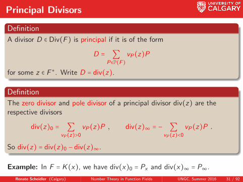
Definition

A divisor D ∈ Div(F ) is principal if it is of the form

D = ∑P∈P(F)

vP(z)P

for some z ∈ F ∗. Write D = div(z).

Definition

The zero divisor and pole divisor of a principal divisor div(z) are therespective divisors

div(z)0 = ∑vP(z)>0

vP(z)P , div(z)∞ = − ∑vP(z)<0

vP(z)P .

So div(z) = div(z)0 − div(z)∞.

Example: In F = K(x), we have div(x)0 = Px and div(x)∞ = P∞.


More on Principal Divisors

Theorem

Let x ∈ F ∖K . Then deg(div(x)0) = deg(div(x)∞) = [F ∶ K(x)].It follows that deg(div(z)) = 0, so the principal divisors form a subgroup ofDiv0(F ), denoted Prin(F ).

Definition

Two divisors D1,D2 ∈ Div(F ) are (linearly) equivalent, denoted D1 ∼ D2, ifD1 −D2 ∈ Prin(F ).

Remark and Notation

Linear equivalence is an equivalence relation. The class of a divisor Dunder linear equivalence is denoted [D].


Class Group and Zero Class Group

Definition

The factor groups

Cl(F ) = Div(F )/Prin(F ) and Cl0(F ) = Div0(F )/Prin(F )

are the divisor class group and the degree zero divisor class group of F /K ,respectively. (Usually abbreviated to just class group and zero class group.)

Remarks and Definition

Both Cl(F ) and Cl0(F ) are abelian groups.

Cl(F ) is always infinite, but Cl0(F ) may or may not be infinite. It itis finite, then the order hF is called the degree zero divisor classnumber (or just class number) of F /K . We will see later on that hFis always finite for a function field over a finite field.

Sometimes the zero class group is also called the Jacobian of F /K .


More on Class Groups

Theorem

Every rational function field has class number one.

Remark

There are 8 non-rational function fields F /Fq of class number one. Allhave q ≤ 4, and defining curves for all of them are known.

Theorem

Let F /K be a non-rational function field that has a rational place,denoted P∞. Then the map Φ ∶ P1(F )→ Cl0(F ) via P ↦ [P − P∞] isinjective.

The above embedding imposes an abelian group structure on P1(F ). Notethat this group structure is non-canonical (depends on the choice of P∞).


Effective Divisors

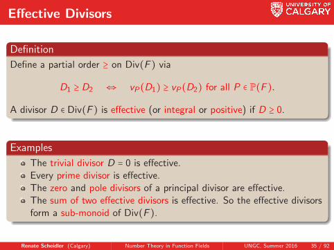
Definition

Define a partial order ≥ on Div(F ) via

D1 ≥ D2 ⇔ vP(D1) ≥ vP(D2) for all P ∈ P(F ).

A divisor D ∈ Div(F ) is effective (or integral or positive) if D ≥ 0.

Examples

The trivial divisor D = 0 is effective.Every prime divisor is effective.The zero and pole divisors of a principal divisor are effective.The sum of two effective divisors is effective. So the effective divisorsform a sub-monoid of Div(F ).


Riemann-Roch Spaces

Definition

The Riemann-Roch space of a divisor D ∈ Div(F ) is the set

L(D) = {x ∈ F ∣ div(x) +D ≥ 0} ∪ {0}.

Interpretation

L(D) consists of all x ∈ F such that

If D has a pole of order m at P, then x has a zero of order at least mat P.

If D has a zero of order m at P, then x may have a pole at P, but itsorder cannot exceed m.


Examples

Examples

Let F = K(x).

L(nP∞) = {f (x) ∈ K [x] ∣ deg(f ) ≤ n} for n ≥ 0.

If D = −3Px−1 + 2Px−2 + 4Px−7, then

L(D) = { (x − 1)3

(x − 2)2(x − 7)4r(x) ∣ r(x) ∈ K(x),deg(r) ≤ 3} .

For any function field F /K , if P ∈ P(F ) and n ∈ Z with n > 0, then

L(nP) ∖ L((n − 1)P) = {x ∈ F ∣ div(x)∞ = nP}.


Properties of Riemann-Roch Spaces

x ∈ L(D) if and only if vP(x) ≥ −vP(D) for all P ∈ P(F ).

L(D) is a K -vector space.

If D1 ∼ D2, then L(D1) ≅ L(D2) (isomorphic as K -vector spaces).

L(0) = K .

If deg(D) < 0 or D ∈ Div0(F ) ∖ Prin(F ), then L(D) = {0}.

L(D) ≠ {0} if and only if the class [D] contains an effective divisor.

Notation

The K -vector space dimension of L(D) is denoted `(D) = dimK(L(D)).

Remark

Both deg(D) and `(D) depend only on the divisor class [D].


Genus

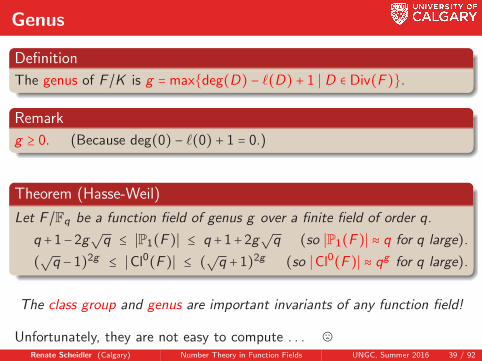
Definition

The genus of F /K is g = max{deg(D) − `(D) + 1 ∣ D ∈ Div(F )}.

Remark

g ≥ 0. (Because deg(0) − `(0) + 1 = 0.)

Theorem (Hasse-Weil)

Let F /Fq be a function field of genus g over a finite field of order q.

q +1−2g√q ≤ ∣P1(F )∣ ≤ q +1+2g

√q (so ∣P1(F )∣ ≈ q for q large).

(√q − 1)2g ≤ ∣Cl0(F )∣ ≤ (√q + 1)2g (so ∣Cl0(F )∣ ≈ qg for q large).

The class group and genus are important invariants of any function field!

Unfortunately, they are not easy to compute . . . /Renate Scheidler (Calgary) Number Theory in Function Fields UNGC, Summer 2016 39 / 92

Riemann-Roch Theorem

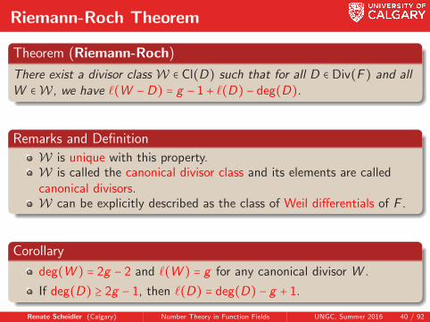
Theorem (Riemann-Roch)

There exist a divisor class W ∈ Cl(D) such that for all D ∈ Div(F ) and allW ∈W, we have `(W −D) = g − 1 + `(D) − deg(D).

Remarks and Definition

W is unique with this property.W is called the canonical divisor class and its elements are calledcanonical divisors.W can be explicitly described as the class of Weil differentials of F .

Corollary

deg(W ) = 2g − 2 and `(W ) = g for any canonical divisor W .

If deg(D) ≥ 2g − 1, then `(D) = deg(D) − g + 1.


Function Field Extensions

Recollection: Prime Ideals in Number Fields

Recall that in a number field extension F ′/F /Q:

A prime ideal p of OF need not remain prime when extended to OF ′ .Rather, it has a prime ideal factorization pOF ′ =Pe1

1 Pe22 ⋯Per

r in OF ′ .

Each Pi is said to lie above p, written Pi ∣p.Finitely many prime ideals of OF ′ lie above any prime ideal of OF .

p is said to lie below each Pi .A unique prime ideal of OF lies below every prime ideal of OF ′ .

ei is called the ramification index of Pi ∣p.

The field extension degree fi = [OF ′/P ∶ OF /p] is called the residuedegree of Pi ∣p.

The norm of Pi is the OF -ideal NF ′/F (Pi) = pfi .The norm extends multiplicatively to all ideals of OF ′ .

The fundamental identityr

∑i=1

ei fi = [F ′ ∶ F ] holds.

Once again, we consider analogous notions in function field extensions,with prime ideals replaced by places, and products replaced by sums.


Function Field Extensions

Notation and Assumption

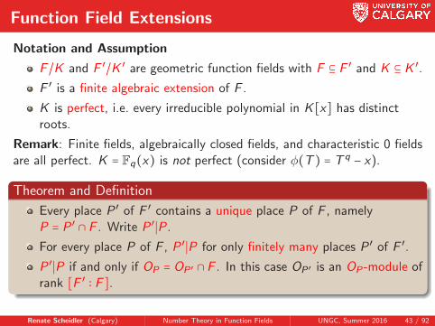
F /K and F ′/K ′ are geometric function fields with F ⊆ F ′ and K ⊆ K ′.

F ′ is a finite algebraic extension of F .

K is perfect, i.e. every irreducible polynomial in K [x] has distinctroots.

Remark: Finite fields, algebraically closed fields, and characteristic 0 fieldsare all perfect. K = Fq(x) is not perfect (consider φ(T ) = T q − x).

Theorem and Definition

Every place P ′ of F ′ contains a unique place P of F , namelyP = P ′ ∩ F . Write P ′∣P.

For every place P of F , P ′∣P for only finitely many places P ′ of F ′.

P ′∣P if and only if OP = OP ′ ∩ F . In this case OP ′ is an OP -module ofrank [F ′ ∶ F ].


Ramification, Residue Degree, Norm and Co-Norm

Theorem and Definition

Let P ∈ P(F ), P ′ ∈ P(F ′) with respective discrete normalized valuationsvP , vP ′ and residue fields FP = OP/P, F ′P ′ = OP ′/P ′. Assume P ′∣P.

There is a unique positive integer e = e(P ′∣P) such thatvP ′(x) = evP(x) for all x ∈ F , called the ramification index of P ′∣P.

There is a natural embedding FP ↪ F ′P ′ via x + P ↦ x + P ′. Theextension degree f (P ′∣P) = [F ′P ′ ∶ FP] is called the residue degree (orrelative degree) of P ′∣P.

The norm of P ′ is the divisor NF ′/F (P ′) = f (P ′∣P)P of F .

The co-norm of P is the divisor conF ′/F (P) = ∑P ′∣P

e(P ′∣P)P ′ of F ′.

The norm and co-norm extend additively to homomorphisms ondivisors and respect principal divisors, so they also extend tohomomorphisms on divisor classes.

∑P ′∣P

e(P ′∣P)f (P ′∣P) = [F ′ ∶ F ] (fundamental identity).


Example — Quadratic Extensions

Let char(K) ≠ 2, F = K(x , y) where x ∈ F is transcendental over K andy2 = f (x) with f (x) ∈ K [x] ∖K 2 square-free.

For any place P ′ of F , with P = P ′ ∩K(x):

2vP ′(y) = vP ′(y2) = vP ′(f ) = e(P ′∣P)vP(f ) .

Case P is finite. Write P = Pp(x) with p(x) ∈ K [x] monic and irreducible.

If p(x) ∤ f (x) then vP ′(y) = 0.

If p(x) ∣ f (x), then vP(f ) = 1 (since f is square-free), so e(P ′∣P) = 2.Then vP ′(y) = 1 and ConF /K(x)(P) = 2P ′.

Case P = P∞. Then vP(f ) = v∞(f ) = −deg(f ).

If deg(f ) is odd, then e(P ′∣P) = 2.Then vP ′(y) = −deg(f ) and ConF /K(x)(P) = 2P ′.

If deg(f ) is even, then we will later see that e(P ′∣P) = 1.Then vP ′(y) = −deg(f )/2.


Extension Terminology

Definition

Let P ∈ P(F ).

If P ′ ∈ P(F ′) with P ′∣P, then P ′ lies above P and P lies below P ′.

P is unramified if e(P ′∣P) = 1 for all P ′∣P and ramified otherwise.

P is wildly ramified if char(K) divides e(P ′∣P) for some P ′P, andtamely ramified otherwise.

P is totally ramified if ConF ′/F (P) = [F ∶ F ′]P ′.

P is inert in F ′ if ConF ′/F (P) = P ′ with f (P ′∣P) = [F ∶ F ′].P splits completely in F ′ if e(P ′∣P) = f (P ′∣P) = 1 for all P ′∣P.

Sufficient (but not necessary) conditions for a function field to be tamelyramified are:

char(K) = 0.

[F ′ ∶ F ] < char(K) when char(K) is positive.)


Properties

Properties relating “Upstairs” to “Downstairs”:

deg(P ′) = f (P ′∣P)[K ′ ∶ K ] deg(P) for all P ∈ P(F ), P ′ ∈ P(F ′) with P ′∣P.

deg(ConF ′/F (D)) = [F ′ ∶ F ][K ′ ∶ K ] deg(D) for all D ∈ Div(F ).

NF ′/F (ConF ′/F (D)) = [F ′ ∶ F ]D for all D ∈ Div(F ).

Transitivity Theorem

Consider F /K , F ′/K ′ and F ′′/K ′′ with F ⊆ F ′ ⊆ F ′′ and K ⊆ K ′ ⊆ K ′′.

Let P ∈ P(F ), P ′ ∈ P(F ′), P ′′ ∈ P(F ′′) with P ′′∣P ′∣P. Thene(P ′′∣P) = e(P ′′∣P ′)e(P ′∣P) and f (P ′′∣P) = f (P ′′∣P ′)f (P ′∣P).

NF ′′/F (D ′′) = NF ′/F (NF ′′/F ′(D ′′)) for all D ′′ ∈ Div(F ′′).

ConF ′′/F (D) = ConF ′′/F ′(ConF ′/F (D)) for all D ∈ Div(F ).


Recollection: Prime Splitting in Number Fields

In number fields, prime decomposition can almost always be obtained from

Kummer’s Theorem (Number Fields)

Let F /Q be a number field and p a prime. Let F = Q(α) such that α ∈ OF

and p does not divide the index [OF ∶ Z[α]]. Let φα(T ) ∈ Z[T ] be theminimal polynomial of α and consider φα(T ) ∈ Fp[T ], the reduction ofφα(T ) modulo p. Let

φα(T ) ≡ φ1(T )e1 φ2(T )e2 ⋯ φr(T )er (mod p)

be the factorization of φα(T ) over Fp into distinct irreducible polynomials.Then the prime ideal factorization of p in OF is

pOF = pe11 pe2

2 ⋯perr ,

where pi = pOF + φi(α)OF , and pi has residue degree fi = deg(φi), for1 ≤ i ≤ r .


Kummer’s Theorem for Function Fields

Kummer’s Theorem (Function Fields)

Let F ′/F be a finite algebraic extension of function fields of degreen = [F ′ ∶ F ] and P ∈ P(F ). Let F ′ = F (y) such that y is integral over OP .Let φy(T ) ∈ OP[T ] be the minimal polynomial of y over F , and considerφy(T ) ∈ Fp[T ], the image of φy(T ) modulo P under the residue mapOP → FP . Let

φy(T ) ≡ φ1(T )ε1 φ2(T )ε2 ⋯ φr(T )εr (mod P)

be the factorization of φy(T ) over FP into distinct irreducible polynomials.Then there are at least r distinct places P ′

1, P′

2, . . . , P′

r ∈ P(F ′) lyingabove P. Furthermore, φi(y) ∈ P ′

i and f (P ′

i ∣P) ≥ deg(φi) for 1 ≤ i ≤ r .

If in addition, {1, y , . . . , yn−1} is an OP -basis of the integral closureOP = ⋂r

i=1 OP ′i in F ′ or εi = 1 for 1 ≤ i ≤ r , then

ConF ′/F (P) = ε1P′

1 + ε2P′

2 +⋯ + εrP ′

r ,

so e(P ′

i ∣P) = εi and f (P ′

i ∣P) = deg(φi) for 1 ≤ i ≤ r .


Example — Quadratic Extensions

Let char(K) ≠ 2, F = K(x , y) where x ∈ F is transcendental over K andy2 = f (x) with f (x) ∈ K [x] ∖K 2 square-free.

A finite place P = Pp(x) of K(x)ramifies in F if p(x) divides f (x);splits in F if f (x) is a square modulo p(x);is inert in F if f (x) is a non-square modulo p(x).

The infinite place of K(x)ramifies in F if deg(f ) is odd;splits in F if deg(f ) is even and sgn(f ) is a square in K∗;is inert in F if deg(f ) is even and sgn(f ) is a non-square in K∗.

E.g. if K = F5 and f (x) = x3 + 3x + 2 = (x + 1)(x + 2) ∈ F5[x], then theramified places of F5(x) are Px+1, Px+2 and P∞.

The place Px2+2x+4 of F5(x) splits in F because

x2 + 2x + 4 = (2x2 + 2)2 + x(x3 + 3x + 2) ≡ (2x2 + 2)2 (mod f (x)) .Renate Scheidler (Calgary) Number Theory in Function Fields UNGC, Summer 2016 50 / 92

The Different

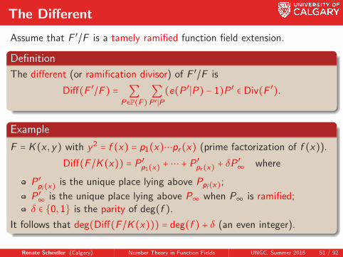
Assume that F ′/F is a tamely ramified function field extension.

Definition

The different (or ramification divisor) of F ′/F is

Diff(F ′/F ) = ∑P∈P(F)

∑P ′∣P

(e(P ′∣P) − 1)P ′ ∈ Div(F ′).

Example

F = K(x , y) with y2 = f (x) = p1(x)⋯pr(x) (prime factorization of f (x)).

Diff(F /K(x)) = P ′

p1(x)+⋯ + P ′

pr (x)+ δP ′

∞where

P ′

pi(x)is the unique place lying above Ppi(x);

P ′

∞is the unique place lying above P∞ when P∞ is ramified;

δ ∈ {0,1} is the parity of deg(f ).

It follows that deg(Diff(F /K(x))) = deg(f ) + δ (an even integer).


Genus and Ramification

Theorem (Hurwitz Genus Formula)

Let F ′/K ′ be a finite algebraic function field extension of F /K , and denoteby gF ′ and gF the genera of F ′ and F , respectively. Then

2gF ′ − 2 = [F ′ ∶ F ][K ′ ∶ K ](2gF − 2) + deg(Diff(F ′/F )).

Corollary

The different has even degree.

If x ∈ F ∖K , then gF = 12 deg(Diff(F /K(x)) − [F ∶ K(x)] + 1.

Example (elliptic and hyperelliptic function fields):F = K(x , y) with char(K) ≠ 2; y2 = f (x) with f (x) ∈ K [x] square-free.

g = ⌊(deg(f ) − 1)/2⌋ (so deg(f ) = 2g + 1 or 2g + 2).

deg(Diff(F /K(x)) = 2g + 2.


Constant Field Extensions

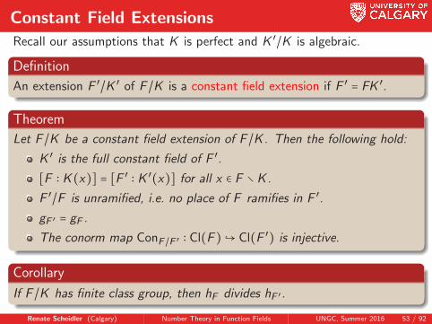
Recall our assumptions that K is perfect and K ′/K is algebraic.

Definition

An extension F ′/K ′ of F /K is a constant field extension if F ′ = FK ′.

Theorem

Let F /K be a constant field extension of F /K . Then the following hold:

K ′ is the full constant field of F ′.

[F ∶ K(x)] = [F ′ ∶ K ′(x)] for all x ∈ F ∖K .

F ′/F is unramified, i.e. no place of F ramifies in F ′.

gF ′ = gF .

The conorm map ConF /F ′ ∶ Cl(F )↪ Cl(F ′) is injective.

Corollary

If F /K has finite class group, then hF divides hF ′ .


Genus 0 and 1 Function Fields

Genus 0 Function FieldsWe continue to assume that K is perfect.

Theorem

Let F /K be a function field of genus 0. Then the following hold:

F /K is rational if and only if it has a rational (i.e. degree 1) place.If F /K is not rational, then F has a place of degree 2, and thereexists x ∈ F with [F ∶ K(x)] = 2.

Corollary

For K algebraically closed, F /K is rational if and only if F has genus 0.

Example

Suppose K does not contain a square root of −1, and let F = K(x , y)where x2 + y2 = −1. Then F has genus 0 but is not rational.

Remark

Every genus 0 function field has class number 1.


Genus 1 Function Fields

Definition

A function field F /K is elliptic if it has genus 1 and a rational place.

Corollary

For K algebraically closed, F /K is elliptic if and only if F has genus 1.

Example

Suppose K does not contain a square root of −1, and let F = K(x , y)where x2 + y4 = −1. Then F has genus 1 but is not elliptic.

Theorem

If F /K is elliptic, then there exist x , y ∈ F such that F = K(x , y) and

y2 + a1xy + a3y = x3 + a2x2 + a4x + a6.

for some a1, a2, a3, a4, a6 ∈ K . This equation defines an elliptic curve inWeierstrass form.

Remark

[F ∶ K(x)] = 2 and [F ∶ K(y)] = 3.


Short Weierstrass Form

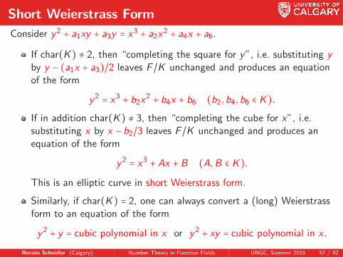
Consider y2 + a1xy + a3y = x3 + a2x2 + a4x + a6.

If char(K) ≠ 2, then “completing the square for y”, i.e. substituting yby y − (a1x + a3)/2 leaves F /K unchanged and produces an equationof the form

y2 = x3 + b2x2 + b4x + b6 (b2,b4,b6 ∈ K).

If in addition char(K) ≠ 3, then “completing the cube for x”, i.e.substituting x by x − b2/3 leaves F /K unchanged and produces anequation of the form

y2 = x3 +Ax +B (A,B ∈ K).

This is an elliptic curve in short Weierstrass form.

Similarly, if char(K) = 2, one can always convert a (long) Weierstrassform to an equation of the form

y2 + y = cubic polynomial in x or y2 + xy = cubic polynomial in x .


Interlude – Why “Genus”?Brief excursion into the topology and geometry of function fields. ,

In topology, the genus g of a connected, orientable surface is the numberof “handles” on it (or ”holes” in it). It is the maximum number of (closednon-intersecting) cuts that are possible without disconnecting the surface.

For example:

A sphere has genus 0A “doughnut” (torus) has genus 1, as does a coffee mug with a handleA ”pretzel” (3-dimensional figure 8) has genus 2

Geometrically, over an algebraically closed field K , places of a functionfield F /K correspond one-to-one to the points on the unique non-singularplane curve defining F /K .

A rational (i.e. genus 0) function field over C corresponds to theprojective line P1(C), which is a sphere and thus a genus 0 object.

An elliptic (i.e. genus 1) curve over C corresponds to the plane C2

modulo its period lattice which is a torus and thus a genus 1 object.


P1(F ) as an Abelian Group

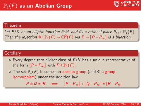
Theorem

Let F /K be an elliptic function field, and fix a rational place P∞ ∈ P1(F ).Then the injection Φ ∶ P1(F )→ Cl0(F ) via P ↦ [P − P∞] is a bijection.

Corollary

Every degree zero divisor class of F /K has a unique representative ofthe form [P − P∞] with P ∈ P1(F ).

The set P1(F ) becomes an abelian group (and Φ a groupisomorphism) under the addition law

P ⊕Q =∶ R ⇐⇒ [P − P∞] + [Q − P∞] = [R − P∞].


Points on an Elliptic Curve

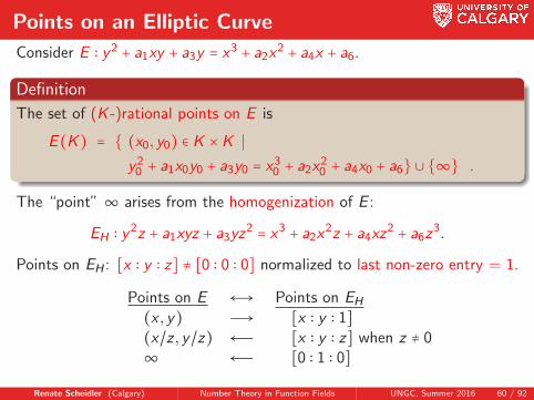
Consider E ∶ y2 + a1xy + a3y = x3 + a2x2 + a4x + a6.

Definition

The set of (K -)rational points on E is

E(K) = { (x0, y0) ∈ K ×K ∣y2

0 + a1x0y0 + a3y0 = x30 + a2x

20 + a4x0 + a6} ∪ {∞} .

The “point” ∞ arises from the homogenization of E :

EH ∶ y2z + a1xyz + a3yz2 = x3 + a2x

2z + a4xz2 + a6z

3.

Points on EH : [x ∶ y ∶ z] ≠ [0 ∶ 0 ∶ 0] normalized to last non-zero entry = 1.

Points on E ←→ Points on EH

(x , y) Ð→ [x ∶ y ∶ 1](x/z , y/z) ←Ð [x ∶ y ∶ z] when z ≠ 0∞ ←Ð [0 ∶ 1 ∶ 0]


Point Arithmetic

Theorem (Bezout)

Two curves of respective degrees m and n intersect in exactly mn points(counting point multiplicities).

Corollary

A line intersects an elliptic curve in exactly 3 points.

Group Law on E(K) (additive, abelian):

Identity: ∞.

Inverses: −p is defined as the third point of intersection of the“vertical”line through p and ∞ with E .Addition:

▸ If p ≠ q, then −r is defined as the third point of intersection ofthe secant line through p and q with r .

▸ If p = q, then −r is defined as the third point of intersection ofthe tangent line at p to E .

▸ Must then invert −r to obtain r .Renate Scheidler (Calgary) Number Theory in Function Fields UNGC, Summer 2016 61 / 92

An Elliptic Curve and a Point

E ∶ y2 = x3 − 5x over Q, p = (-1, -2) ∈ E(Q)

-10

-5

0

5

10

-3 -2 -1 0 1 2 3 4 5 6


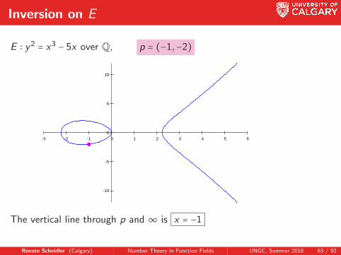
Inversion on E

E ∶ y2 = x3 − 5x over Q, p = (−1,−2)

-10

-5

0

5

10

-3 -2 -1 0 1 2 3 4 5 6

The vertical line through p and ∞ is x = −1


Inversion on E

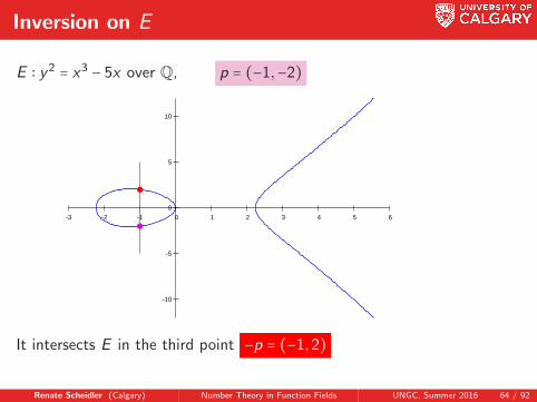
E ∶ y2 = x3 − 5x over Q, p = (−1,−2)

-10

-5

0

5

10

-3 -2 -1 0 1 2 3 4 5 6

It intersects E in the third point −p = (−1,2)


Addition of Distinct Points on E

E ∶ y2 = x3 − 5x over Q, p = (−1,−2), q = (0,0)

-10

-5

0

5

10

-3 -2 -1 0 1 2 3 4 5 6

The line through p and q is y = 2x



E ∶ y2 = x3 − 5x over Q, p = (−1,−2), q = (0,0)

-10

-5

0

5

10

-3 -2 -1 0 1 2 3 4 5 6

It intersects E in the third point −r = (5,10)



E ∶ y2 = x3 − 5x over Q, p = (−1,−2), q = (0,0)

-10

-5

0

5

10

-3 -2 -1 0 1 2 3 4 5 6

The sum r = p + q is the inverse of −r , i.e. r = (5,−10)


Doubling on E

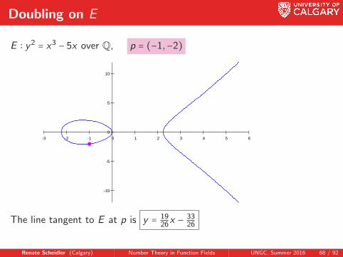
E ∶ y2 = x3 − 5x over Q, p = (−1,−2)

-10

-5

0

5

10

-3 -2 -1 0 1 2 3 4 5 6

The line tangent to E at p is y = 1926x −

3326


Doubling on E

E ∶ y2 = x3 − 5x over Q, p = (−1,−2)

-10

-5

0

5

10

-3 -2 -1 0 1 2 3 4 5 6

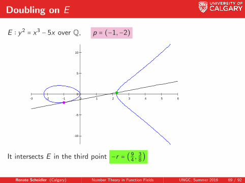
It intersects E in the third point −r = (94 ,

38)


Doubling on E

E ∶ y2 = x3 − 5x over Q, p = (−1,−2)

-10

-5

0

5

10

-3 -2 -1 0 1 2 3 4 5 6

The sum r = p + p is the inverse of −r , i.e. r = (94 ,−

38)


Rational Points and Rational Places

Recall the addition law on P1(F ):

P ⊕Q = R ⇔ [P − P∞] + [Q − P∞] = [R − P∞]⇔ [P] + [Q] − [R] = [P∞]

Recall the addition law on E(K): p + q − r =∞.

Theorem

Let (x0, y0) ∈ E(K) ∖ {∞}. Then exists a unique P(x0,y0)∈ P1(F )

such that supp(div(x − x0)) ∩ supp(div(y − y0)) = {P(x0,y0),P∞}.

The map Ψ ∶ E(K)→ P1(K) via (x0, y0)↦ P(x0,y0)and ∞↦ P∞ is a

group isomorphism.

So we have group isomorphisms

(E(K), point addition)Ψ←→ (P1(F ),⊕) Φ←→ (Cl0(F ), divisor addition)


Hyperelliptic Function Fields

Hyperelliptic Function Fields

Definition

A function field F /K is hyperelliptic if it has genus at least 2 and thereexists x ∈ F such that [F ∶ K(x)] = 2.

Properties:

F /K is hyperelliptic if and only if there exists D ∈ Div(F ) withdeg(D) = 2 and `(D) ≥ 2.Every genus 2 function field is hyperelliptic.

Description: Write F = K(x , y) with [F ∶ K(x)] = 2.Then F /K(x) has a minimal polynomial of the form

y2 + h(x)y = f (x)

where h(x) and f (x) are polynomials (after we make everything integral)and h(x) = 0 if K has characteristic ≠ 2.


Hyperelliptic Curves

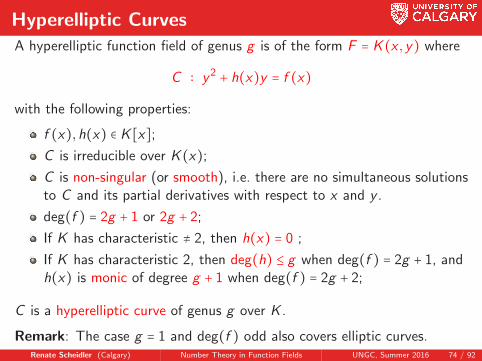
A hyperelliptic function field of genus g is of the form F = K(x , y) where

C ∶ y2 + h(x)y = f (x)

with the following properties:

f (x),h(x) ∈ K [x];C is irreducible over K(x);

C is non-singular (or smooth), i.e. there are no simultaneous solutionsto C and its partial derivatives with respect to x and y .

deg(f ) = 2g + 1 or 2g + 2;

If K has characteristic ≠ 2, then h(x) = 0 ;

If K has characteristic 2, then deg(h) ≤ g when deg(f ) = 2g + 1, andh(x) is monic of degree g + 1 when deg(f ) = 2g + 2;

C is a hyperelliptic curve of genus g over K .

Remark: The case g = 1 and deg(f ) odd also covers elliptic curves.Renate Scheidler (Calgary) Number Theory in Function Fields UNGC, Summer 2016 74 / 92

Examples

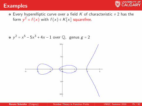
Every hyperelliptic curve over a field K of characteristic ≠ 2 has theform y2 = f (x) with f (x) ∈ K [x] squarefree.

y2 = x5 − 5x3 + 4x − 1 over Q, genus g = 2

-10

-5

0

5

10

-3 -2 -1 0 1 2 3


Classification by to Splitting at Infinity

Case 1: deg(f ) = 2g + 1 (odd). Then P∞ ramifies in F .

Case 2: deg(f ) = 2g + 2 (even) and

sgn(f ) is a square in K∗ when q is odd;sgn(f ) is of the form s2 + s for some s ∈ K when q is even.

Then P∞ splits in F .

Case 3: deg(f ) = 2g + 2 (even) and

sgn(f ) is a non-square in K∗ when q is odd;sgn(f ) is not of the form s2 + s with s ∈ K when q is even.

Then P∞ is inert in F .

The representation of F /K(x) by C is referred to as ramified, split, andinert according to these three cases, or alternatively as imaginary, real, andunusual.


Model Properties

Ramified representations are the function field analogue of imaginaryquadratic number fields. Split representations are the function fieldanalogue of real quadratic number fields. Inert representations haveno number field analogue.

The variable transformation x ↦ 1/(x − a) and y ↦ y/(x − a)g+1, withf (a) ≠ 0, converts a ramified representation of F /K(x) into a split orinert representation of F /K(x) without changing the underlyingrational function field K(x).

The same variable transformation, with f (a) = 0, converts an inert orsplit representation of F /K(x) into a ramified representation ofF (a)/K(a)(x); note that this may require an extension of theconstant field.

Inert models F /K(x) become split when considered over a quadraticextension over K . They don’t exist over algebraically closed fields.


Degree Zero Divisors

Let D ∈ Div0(F ).

Ramified model: ConF /K(x)(P∞) = 2∞ with deg(∞) = 1.

D = D0 − deg(D0)∞ with ∞ ∉ supp(D0) .

This gives rise to a group isomorphism from Div0(F ) onto the group offinite divisors {D ∈ Div(F ) ∣∞ ∉ supp(D)}.

Split model: ConF /K(x)(P∞) =∞+ +∞− with deg(∞+) = deg(∞−) = 1.

D = D0 − deg(D0)∞− − n(∞+ −∞−) with ∞+,∞− ∉ supp(D0) and n ∈ Z .

This gives rise to a surjective group homomorphism from Div0(F ) ontothe group of finite divisors {D ∈ Div(F ) ∣∞+,∞− ∉ supp(D)} with kernel⟨∞+ −∞−⟩.

Henceforth concentrate on finite divisors.Renate Scheidler (Calgary) Number Theory in Function Fields UNGC, Summer 2016 78 / 92

Semi-Reduced and Reduced Divisors

Definition

A finite divisor D of F is semi-reduced if it is

effective, i.e. vP(D) ≥ 0 for all P ∈ P(F ), and

co-norm-free, i.e. can’t be written as D = E +A where A is thecon-norm of some divisor of K(x).

D is reduced if it is semi-reduced and deg(D) ≤ g .

Proposition

A finite divisor is semi-reduced if and only if D is effective and for anyP ∈ supp(D), the following hold:

If P ∩K is inert in F , then vP(D) = 0.

If P ∩K is ramified in F , then vP(D) = 1.

If P ∩K splits in F , say as P +Q, then either vP(D) = 0 or vQ(D) = 0.


More on Semi-Reduced Divisors

Lemma

Every class in Cl0(F ) contains a divisor whose finite part is semi-reduced.

Theorem

Every class in Cl0(F ) contains a divisor D whose finite part D0 isreduced.

If [F ∶ K(x)] is ramified, then D is unique.

If [F ∶ K(x)] is split, then there is a unique such divisor D with0 ≤ n ≤ g − deg(D0). All but at most g classes have n = 0, i.e.D = D0 − deg(D0)∞+.

Remark

If [F ∶ K(x)] is split, then the divisors D = D0 − deg(D0)∞+ form theinfrastructure of F /K(x) (more on that later).


Mumford Representation of Places

Write F = K(x , y)] with y2 + h(x)y = f (x).

Lemma

Let P be a finite place of F , and write P ∩K(x) = Pp(x) withp(x) ∈ K [x] monic and irreducible. Suppose Pp(x) ramifies or splits inF . Then there exists a polynomial v(x) ∈ K [x], unique modulo p(x),with v(x)2 + h(x)v(x) ≡ f (x) (mod p(x)) and vP(v + y) > 0. .

Conversely, let p(x), v(x) ∈ K [x] with p(x) be monic and irreducible,and v(x)2 + h(x)v(x) ≡ f (x) (mod p(x)). Then Pp(x) ramifies orsplits in F and there exists a unique finite place P of F lying abovePp(x) with vP(v + y) > 0.

Corollary

The polynomials (p(x), v(x) mod p(x)) as above are in one-to-onecorrespondence with the finite places P of F such that P ∩K(x) ramifiesor splits in F .


Mumford Representation of of Divisors

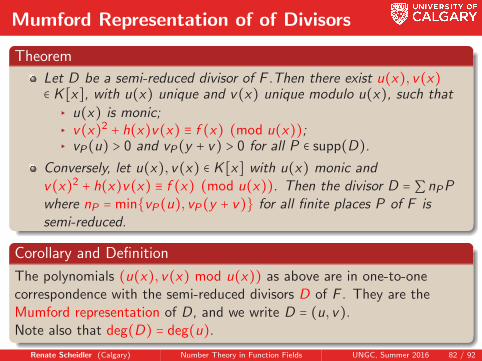
Theorem

Let D be a semi-reduced divisor of F .Then there exist u(x), v(x)∈ K [x], with u(x) unique and v(x) unique modulo u(x), such that

▸ u(x) is monic;▸ v(x)2 + h(x)v(x) ≡ f (x) (mod u(x));▸ vP(u) > 0 and vP(y + v) > 0 for all P ∈ supp(D).

Conversely, let u(x), v(x) ∈ K [x] with u(x) monic andv(x)2 + h(x)v(x) ≡ f (x) (mod u(x)). Then the divisor D = ∑nPPwhere nP = min{vP(u), vP(y + v)} for all finite places P of F issemi-reduced.

Corollary and Definition

The polynomials (u(x), v(x) mod u(x)) as above are in one-to-onecorrespondence with the semi-reduced divisors D of F . They are theMumford representation of D, and we write D = (u, v).Note also that deg(D) = deg(u).


Examples of Mumford Representations

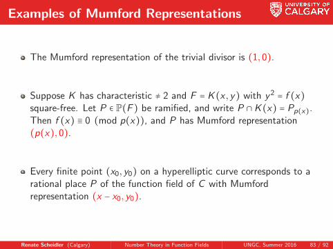
The Mumford representation of the trivial divisor is (1,0).

Suppose K has characteristic ≠ 2 and F = K(x , y) with y2 = f (x)square-free. Let P ∈ P(F ) be ramified, and write P ∩K(x) = Pp(x).Then f (x) ≡ 0 (mod p(x)), and P has Mumford representation(p(x),0).

Every finite point (x0, y0) on a hyperelliptic curve corresponds to arational place P of the function field of C with Mumfordrepresentation (x − x0, y0).


Semi-reduced Divisors and K [x , y]-ideals

Theorem

Let u(x), v(x) ∈ K [x]. Then the following are equivalent:

(u, v) is the Mumford representation of a reduced divisor of F .

The K [x]-submodule of K [x , y] of rank 2 generated by u(x) andv(x) + y is an ideal of K [x , y].v(x)2 + h(x)v(x) ≡ f (x) (mod u(x)).

Remark

If F /K(x) is ramified, then the bijection between semi-reduced divisorsand K [x , y]-ideals of the form above extends to a group isomorphism fromCl0(F ) onto the ideal class group of K [x , y].


Arithmetic in Cl0(F ) for Ramified Models F /K(x)Goal: efficient arithmetic on Cl0(F ) via unique reduced divisor classrepresentatives in Mumford representations when F /K(x) is ramified:

[D1] + [D2] = [D1 ⊕D2] where

D1 and D2 are the unique reduced divisors in their respective classes;

D1 ⊕D2 is the unique reduced divsor in the class of D1 +D2;

All three divisors are given in Mumford representation.

Road map:

1 First compute a semi-reduced divisor D equivalent to D1 +D2 inMumford representation.

2 Then reduce D, i.e. compute the Mumford representation of theunique reduced divisor D1 ⊕D2 equivalent to D.


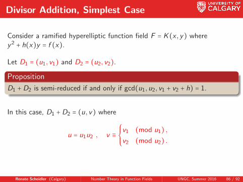
Divisor Addition, Simplest Case

Consider a ramified hyperelliptic function field F = K(x , y) wherey2 + h(x)y = f (x).

Let D1 = (u1, v1) and D2 = (u2, v2).

Proposition

D1 +D2 is semi-reduced if and only if gcd(u1,u2, v1 + v2 + h) = 1.

In this case, D1 +D2 = (u, v) where

u = u1u2 , v ≡⎧⎪⎪⎨⎪⎪⎩

v1 (mod u1) ,v2 (mod u2) .


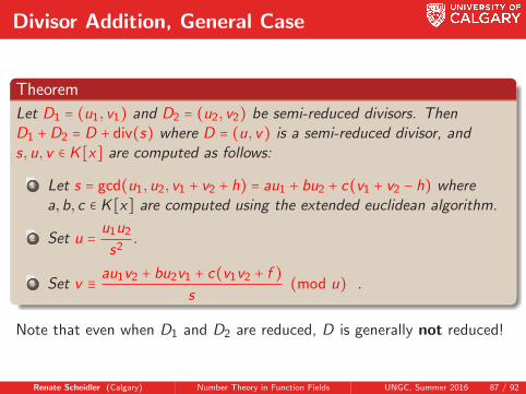
Divisor Addition, General Case

Theorem

Let D1 = (u1, v1) and D2 = (u2, v2) be semi-reduced divisors. ThenD1 +D2 = D + div(s) where D = (u, v) is a semi-reduced divisor, ands,u, v ∈ K [x] are computed as follows:

1 Let s = gcd(u1,u2, v1 + v2 + h) = au1 + bu2 + c(v1 + v2 − h) wherea,b, c ∈ K [x] are computed using the extended euclidean algorithm.

2 Set u = u1u2

s2.

3 Set v ≡ au1v2 + bu2v1 + c(v1v2 + f )s

(mod u) .

Note that even when D1 and D2 are reduced, D is generally not reduced!


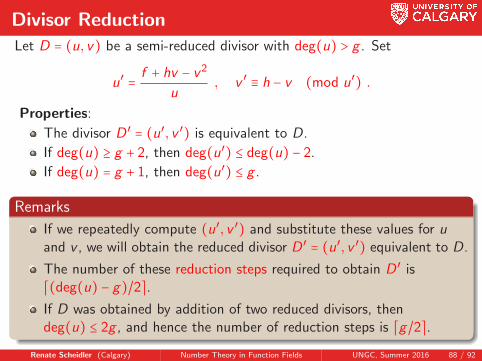
Divisor Reduction

Let D = (u, v) be a semi-reduced divisor with deg(u) > g . Set

u′ = f + hv − v2

u, v ′ ≡ h − v (mod u′) .

Properties:

The divisor D ′ = (u′, v ′) is equivalent to D.

If deg(u) ≥ g + 2, then deg(u′) ≤ deg(u) − 2.

If deg(u) = g + 1, then deg(u′) ≤ g .

Remarks

If we repeatedly compute (u′, v ′) and substitute these values for uand v , we will obtain the reduced divisor D ′ = (u′, v ′) equivalent to D.

The number of these reduction steps required to obtain D ′ is⌈(deg(u) − g)/2⌉.If D was obtained by addition of two reduced divisors, thendeg(u) ≤ 2g , and hence the number of reduction steps is ⌈g/2⌉.


Inert Models

One infinite degree 2 place ∞.

Properties:

If F /K(x) is inert and L is a quadratic extension of K , then FL/L(x)is split.

Only the finite divisors of even degree correspond to degree zerodivisors D0 − (deg(D0)/2)∞.

If K = Fq, then very degree zero divisor class contains either a uniquereduced representative or q + 1 almost reduced divisors (semi-reducedand deg(D0) = g + 1, Artin 1924).

Reduction finds the reduced or an almost reduced representative.For the latter case, Artin provided a procedure for finding the other qalmost reduced equivalent divisors.


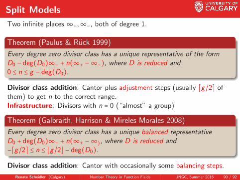
Split Models

Two infinite places ∞+,∞−, both of degree 1.

Theorem (Paulus & Ruck 1999)

Every degree zero divisor class has a unique representative of the formD0 − deg(D0)∞− + n(∞+ −∞−), where D is reduced and0 ≤ n ≤ g − deg(D0).

Divisor class addition: Cantor plus adjustment steps (usually ⌈g/2⌉ ofthem) to get n to the correct range.Infrastructure: Divisors with n = 0 (“almost” a group)

Theorem (Galbraith, Harrison & Mireles Morales 2008)

Every degree zero divisor class has a unique balanced representativeD0 + deg(D0)∞− + n(∞+ −∞), where D is reduced and−⌈g/2⌉ ≤ n ≤ ⌊g/2⌋ − deg(D0).

Divisor class addition: Cantor with occasionally some balancing steps.


Why Consider Split Representations?

Advantages:

A ramified representation need not always exist.

Construction methods (e.g. for cryptography) don’t always produceramified models.

Ramified F /K(x) models can be converted to split models F /K(x),but the reverse direction is only possible over a base field thatcontains a rational point.

Mathematically interesting.

Less researched than ramified models.

Disadvantages:

Mathematically more complicated than ramified models.

Arithmetic is slightly slower.

Less researched than ramified models.


𝒚𝒚𝟐𝟐=𝒙𝒙𝟔𝟔+𝒙𝒙𝟐𝟐+𝒙𝒙

The End

http://voltage.typepad.com/superconductor/2011/09/a-projective-imaginary-hyperelliptic-curve.html

algorithmic number theory in function fields€¦ · algorithmic number theory in function fields...

Documents