Contents lists available at ScienceDirect

Journal of Statistical Planning and Inference

Journal of Statistical Planning and Inference 149 (2014) 172–182

http://d0378-37

n CorrE-m1 Pr

journal homepage: www.elsevier.com/locate/jspi

Algorithmic search for baseline minimum aberration designs

Pei Li a,1, Arden Miller b,n, Boxin Tang a

a Department of Statistics and Actuarial Science Simon Fraser University, 8888 University Drive, Burnaby, British Columbia,Canada V5A 1S6b Department of Statistics, University of Auckland, Private Bag 92019, Auckland 1142, New Zealand

a r t i c l e i n f o

Article history:Received 6 November 2013Received in revised form17 February 2014Accepted 17 February 2014Available online 26 February 2014

Keywords:Baseline modelMinimum aberrationOrthogonal arraySearch algorithmTwo-level design

x.doi.org/10.1016/j.jspi.2014.02.00958 & 2014 Elsevier B.V. All rights reserved.

esponding author. Tel.: þ64 9 373 7599x85ail addresses: crystal.pei.li@gmail.com (P. Li)esent address: Syreon, 260 – 1401 West 8th

a b s t r a c t

This paper reviews the formulation of the K-aberration criterion for baseline two-leveldesigns and the efficient complete search algorithm developed by Mukerjee and Tang(2012). An efficient incomplete search algorithm is proposed that can be used to find nearoptimal baseline designs in situations where the complete search algorithm is not feasible.Lower bounds for values of K2 and K3 are established. A catalogue of optimal (or nearoptimal) 20-run baseline designs is provided.

& 2014 Elsevier B.V. All rights reserved.

1. Introduction

Two level factorial and fractional factorial designs have been extensively studied since the pioneering work of Fisher andYates. The study of optimal fractional factorial designs under the minimum aberration and related model robustness criteriahas received significant attention over the last two decades, motivated by the wide applicability of these designs. Mukerjeeand Wu (2006) provided a survey which concentrates on the so-called regular designs that arise through a definingequation. Recent work in this area has focused on nonregular designs and an excellent review is available in Xu et al. (2009).Both regular and nonregular two-level factorial designs have been of particular interest because of their popularity amongpractitioners. The most common approach to analysing data from a regular two-level fractional factorial design is toestimate a set of contrasts (main effects and interaction effects) as described by Box and Hunter (1961). For a 2m design thesecontrasts form an orthogonal set and thus the estimates are independent – in this paper we will refer to this as theorthogonal parameterization. For a regular fraction of a 2m design (i.e. a 2m�p design) any two effects are either orthogonal toeach other or completely aliased with each other. The aberration criteria are often used to evaluate the extent of aliasing in agiven 2m�p design. In general it is desirable to have as little aliasing as possible between low-order effects and the minimumaberration design achieves this goal.

A less common but in some situations a more natural approach is the baseline parameterization. A baseline parameteriza-tion is natural if there is a null state or baseline level for each factor. For instance, in a toxicological study involving binary

053; fax: þ64 9 373 7018., a.miller@auckland.ac.nz, miller@stat.auckland.ac.nz (A. Miller), boxint@sfu.ca (B. Tang).Ave, Vancouver, BC, Canada V6H 1C9.

P. Li et al. / Journal of Statistical Planning and Inference 149 (2014) 172–182 173

factors that indicate the presence or the absence of a particular toxin, the state of absence can be regarded as a natural baselinelevel for each factor (Kerr, 2006). A baseline level need not strictly mean the zero level on some scale, but can also refer to astandard or control level. Thus, as noted by Banerjee and Mukerjee (2008), in an industrial experiment on possible qualityimprovement via a change in the settings of several machines, the current settings may constitute the baseline levels.Similarly, in an agricultural experiment to investigate possible improvement in productivity by changing the doses of severalfertilizers, the currently used doses may be considered as baseline levels.

Under the baseline parameterization, Mukerjee and Tang (2012) developed a design theory of optimality and robustnessfor estimating main effects. They first showed that orthogonal arrays of strength two are universally optimal for estimatingmain effects. If interactions cannot be safely ignored, consequently causing bias in the estimation of main effects, Mukerjeeand Tang (2012) proposed an aberration criterion that aims at minimizing this bias in a sequential fashion. Through acomplete search, they found all minimum aberration baseline designs for up to 16 runs.

The present paper has two goals. The first is to provide an expository account of the theory of baseline designs in amanner that is friendly to practitioners. Such effort should help promote the applications of the ideas and methods from thebaseline parameterization, which we think is more appropriate than the orthogonal parameterization in many practicalsituations. Sections 2 and 3 and the description of the complete search algorithm in Section 4 constitute a user-friendlyreview of the foundational work of Mukerjee and Tang (2012). The second goal is to find minimum aberration baselinedesigns for larger run sizes. For designs of 20 runs, we obtain minimum aberration baseline designs for up to 13 factors by acomplete search of all possible designs. In Section 4, we develop a novel incomplete search algorithm that enabled us to findgood designs under the K-aberration criterion for 14 or more factors. By comparing the results from the complete search tothose from our incomplete search algorithm, we conclude that the algorithm performs quite well in identifying designs thatare either optimal or close to optimal with respect to the K-aberration criterion. Section 5 contains a catalogue of theminimum K-aberration 20-run designs that were found using these search algorithms. In Section 6, we establish lowerbounds for values of K2 and K3 for 20-run designs – the methodology we developed to do this can be easily extended toother run sizes. Comparing the values of K3 for the designs found by our incomplete search algorithm to these lower boundsprovides further evidence that the algorithm performs well. Section 7 contains our concluding remarks.

2. The baseline parameterization and the minimum K-aberration criterion

Consider an N-run two-level design inm factors where for each factor, one level has been designated as the baseline level(b) and the other as the test level (t). For the baseline parameterization of the linear model, the main effect of each factor isdefined by a vector of length N which has a zero in the ith position if that factor was set to the baseline level for run i and aone if it was set to the test level. The interaction between two factors is represented by a vector of length N which has a zeroin the ith position if either (or both) of the factors is at its baseline level and a one only if both factors are at their test levels.In general the interaction between g of the factors is a vector that has a zero in the ith position if any of the factors involvedis at its baseline level and a one only if all of the factors are at their test levels. Note that any interaction vector can be easilyobtained by multiplying the main effect vectors for the factors involved in an element-wise fashion – i.e. the ith entry for aninteraction vector is simply the product of the ith entries for the relevant main effect vectors. The set of baseline effects for a23 design is given in Table 1.

Now let θ0 represent the intercept coefficient and θA; θB;…; θABC represent the coefficients for the baseline effectsspecified in Table 1. Then the expected values of the response for a baseline model applied to the 23 design are given inTable 2. The interpretation of the baseline coefficients can be surmised by examining this table. Main effects represent thedifference in the expected response when one factor is changed from the baseline level to the test level while all other factorsare held at the baseline level – e.g. θA ¼ μtbb�μbbb. A two-factor interaction is the difference between the expected responsewhen two factors are set to their test levels and the expected response that would be obtained using an additive maineffects model for these two factors while all other factors are held at the baseline level – e.g. θAB ¼ μttb�μtbb�μbtbþμbbb. Noticethat these interpretations are analogous to those for the coefficients of the orthogonal model with one vital difference: forthe baseline model factors not involved in an effect are fixed at the baseline level whereas for the orthogonal model effects

Table 1Baseline effects for a 23 design.

Factor Baseline effects

A B C A B C AB AC BC ABC

b b b 0 0 0 0 0 0 0t b b 1 0 0 0 0 0 0b t b 0 1 0 0 0 0 0t t b 1 1 0 1 0 0 0b b t 0 0 1 0 0 0 0t b t 1 0 1 0 1 0 0b t t 0 1 1 0 0 1 0t t t 1 1 1 1 1 1 1

Table 2Expected response for a 23 design using the baseline model.

Factor Expected response for thebaseline model

A B C

b b b μbbb ¼ θ0t b b μtbb ¼ θ0þθAb t b μbtb ¼ θ0þθBt t b μttb ¼ θ0þθAþθBþθABb b t μbbt ¼ θ0þθCt b t μtbt ¼ θ0þθAþθCþθACb t t μbtt ¼ θ0þθBþθC þθBCt t t μttt ¼ θ0þθAþθBþθC þθABþθACþθBC þθABC

P. Li et al. / Journal of Statistical Planning and Inference 149 (2014) 172–182174

are defined as being averaged over the remaining factors. For example, the orthogonal model main effect of A is thedifference in the expected response when A is changed from the low level to the high level averaged over the levels of allother factors. The question of under what circumstance might the baseline model be preferred to the (more commonly used)orthogonal model arises. Consider a situation where the baseline levels represent the current settings for the factors of aparticular process and the test levels are being investigated as avenues of possible improvement. Now suppose that forreasons of continuity, the practitioners are reluctant to make wholesale changes to the process and thus wish to identify asmall number of changes that will result in the largest improvement. In such a case, the baseline effects are more relevantthan the orthogonal effects as they are defined in terms of holding the remaining factors at their baseline levels.

We now turn our attention to the main effects only baseline model which will be the focus of the rest of this paper. Themain effects only baseline model for m factors can be represented in matrix form as

Y¼Xθþϵ where ϵ� s2IN : ð1ÞThe model matrix X¼ ½1N Z� is an N � ðmþ1Þmatrix where the first column is all ones and each of the remaining columns isa main effect vector for one of the factors. The first element of the parameter vector θ represents the intercept forthe baseline model and each of the remaining elements represents the main effect coefficient for one of the factors.The estimated parameter vector θ̂ ¼ ½ðXtXÞ�1Xt �Y has covariance matrix s2ðXtXÞ�1. For example, if the design represented inTable 1 is used for a main effects only model, then we have

X¼

1 0 0 01 1 0 01 0 1 01 1 1 01 0 0 11 1 0 11 0 1 11 1 1 1

266666666666664

377777777777775

; θ¼

θ0

θAθB

θC

266664

377775; ðXtXÞ�1 ¼

0:50 �0:25 �0:25 �0:25�0:25 0:50 0:00 0:00�0:25 0:00 0:50 0:00�0:25 0:00 0:00 0:50

26664

37775

If the main effects only baseline model is correct (i.e. all interactions are negligible), then θ̂ ¼ ½ðXtXÞ�1Xt �Y is an unbiasedestimator of θ. The question arises of whether this is the best possible design. Mukerjee and Tang (2012) show that for themodel described in (1), if Z forms a two-symbol orthogonal array of strength two – i.e. for any set of two columns the fourlevel combinations (0, 0), (0, 1), (1, 0) and (1, 1) occur with the same frequency – then the associated design is universallyoptimal among all N-run designs, for inference on θ. Therefore provided that all interactions are negligible, the 23 factorialdesign is optimal. However, if this is not the case then it is necessary to evaluate the impact of the active interactions on theestimates of the main effect coefficients.

The following approach was developed by Mukerjee and Tang (2012). In the presence of active interactions, true model isgiven by

Y¼XθþZ2θ2þ⋯þZmθmþϵ; ð2Þwhere Zj is the model matrix for the j-factor interactions. By applying least square estimation for the main effects model tothis true model, the expected value of θ̂ is

Eðθ̂Þ ¼ ðXtXÞ�1XtðXθþZ2θ2þ⋯þZmθmÞ

¼ θþ ∑m

2ðXtXÞ�1XtZjθj:

The contribution to the bias in θ̂ attributable to active j-factor interactions is ðXtXÞ�1XtZjθj. The first row of the matrixðXtXÞ�1XtZj determines the bias in the intercept estimate and each of the remaining rows determines the bias in one of themain effect estimates. Since the intercept term is usually of little concern, we drop the first row and denote the matrix

Table 3Baseline effects for an eight-run one-factor-at-a-time design.

Factor Baseline effects

A B C A B C AB AC BC ABC

b b b 0 0 0 0 0 0 0b b b 0 0 0 0 0 0 0t b b 1 0 0 0 0 0 0t b b 1 0 0 0 0 0 0b t b 0 1 0 0 0 0 0b t b 0 1 0 0 0 0 0b b t 0 0 1 0 0 0 0b b t 0 0 1 0 0 0 0

P. Li et al. / Journal of Statistical Planning and Inference 149 (2014) 172–182 175

formed by the remaining m rows as Bj. Thus the bias in the estimated main effect coefficients induced by active j-factorinteractions is determined by Bjθj.

Going back to the 23 design represented in Table 1:

Z2 ¼

0 0 00 0 00 0 01 0 00 0 00 1 00 0 11 1 1

266666666666664

377777777777775

; Z3 ¼

00000001

266666666666664

377777777777775

; B2θ2 ¼0:5 0:5 00:5 0 0:50 0:5 0:5

264

375

θABθACθBC

264

375; B3θ3 ¼

0:250:250:25

264

375θABC :

Thus the bias in θ̂A is 0:5θABþ0:5θACþ0:25θABC the bias in θ̂B is 0:5θABþ0:5θBCþ0:25θABC and the bias in θ̂C is0:5θACþ0:5θBCþ0:25θABC .

It is possible to construct an eight-run design for three factors such that the main effects only baseline model can beestimated and that the main effect estimates are unbiased even if some or all of the interactions are active. This would bedone by using a one-factor-at-a-time design – the runs and baseline effects for such a design are given in Table 3. It is easy tosee that for this design both B2 and B3 are zero matrices. For this design, the covariance matrix for the estimated coefficientsis given by

ðXtXÞ�1s2 ¼

0:5 �0:5 �0:5 �0:5�0:5 1:0 0:5 0:5�0:5 0:5 1:0 0:5�0:5 0:5 0:5 1:0

26664

37775s2:

Therefore, although this design results in unbiased main effect estimates in the presence of active interactions, the variancesof those estimates are twice as large as for the 23 design. Clearly a trade-off has to be made between the bias caused byactive interactions and the variance of the estimates. As the values of the interaction coefficients are not known, it is notpossible to evaluate which design would produce main effect estimates with less mean square error. This suggests twopossible approaches to finding optimal baseline designs. One approach would be to restrict the search to “no bias” main-effects-only designs and from these to select the design that optimized some measure of the overall precision of theestimated main effects. A second approach would be to restrict the search to main-effects-only designs that are optimalwith respect to some measure of the overall precision of the estimated main effects and from these to select a design thatminimizes the impact of active interactions. Mukerjee and Tang (2012) argued that given the well known empiricalprinciples of effect hierarchy (interaction effects are less likely to be non-negligible than main effects) and effect sparsity(only a fraction of the interaction effects will be active) the second approach will often be preferable.

In this paper the second approach is adopted following the minimum K-aberration procedure developed by Mukerjeeand Tang (2012). First the set of designs is restricted to two-symbol orthogonal arrays of strength two – as mentioned earliersuch designs are universally optimal for inference on θ for the main-effects-only baseline model. We use OA(N, m, 2, 2) todenote a two-symbol orthogonal array of strength two with N runs and m factors. Now the goal is to minimize the biascaused by B2θ2þB3θ3þ⋯þBmθm. As the θj's are not known, it is sensible to use a design that minimizes the overall size ofthe Bj's. Mukerjee and Tang (2012) propose using Kj ¼ trðBjB

tj Þ as such a measure – note that this trace is equal to the sum of

the squared elements of Bj. Applying the usual effect hierarchy principle (Wu and Hamada, 2009, pp. 172–3), which statesthat interactions of the same order are equally likely to be active and that lower order interactions are more likely to be

P. Li et al. / Journal of Statistical Planning and Inference 149 (2014) 172–182176

active than higher order ones, we look for a design that sequentially minimizes K2, K3, …, Km. Formally we adopt thefollowing definition:

Definition 1. Consider two N-run designs d1 and d2, both given by orthogonal arrays of strength 2. Let s be the smallestinteger s for which the values of Ks for d1 and d2 differ. If the value of Ks for d1 is less than that for d2, then d1 is said to haveless K-aberration than d2. A minimum K-aberration design is one such that no other design has less K-aberration than it.

Note that a consequence of restricting designs to orthogonal arrays of strength 2 is that the run size of such designs islimited to multiples of four: N¼4t where t is a positive integer.

3. Isomorphism for baseline designs

An interesting issue arises in considering isomorphism among designs when using baseline parameterization. Thestandard definition of isomorphism allows for the relabelling of levels but under baseline parameterization the control leveland the test level are not interchangeable. As a result two designs which are isomorphic using the standard definition (andtherefore have equivalent properties relative to the orthogonal parameterization) may have different properties relative tothe baseline parameterization. Thus when considering baseline designs it is necessary to alter the definition of isomorphismas follows:

Definition 2. Two designs are isomorphic if the array Z of one can be obtained from that of the other by row and columnpermutations.

This definition is suitable for baseline designs since K2, …, Km remain unaltered under row and column permutations of Zbut not necessarily under symbol interchange in one or more columns. In the following sections it will be necessary to alsoconsider orthogonal arrays which are nonisomorphic using the standard definition. In order to distinguish between the twotypes of isomorphism we adopt the following definition:

Definition 3. Two orthogonal arrays are combinatorially isomorphic if one can be obtained from the other by row andcolumns permutations and the renaming of symbols in one or more columns.

Obviously, the two definitions are closely related with the definition of combinatorially isomorphic allowing labelinterchanges in addition to all of the operations allowed by the definition of isomorphic. As a result, any two designs that areisomorphic must also be combinatorially isomorphic but that the converse is not true. It follows that the complete set ofnonisomorphic designs S1 is at least as large as the complete set of combinatorially nonisomorphic designs S2 and that eachelement of S1 is combinatorially isomorphic to exactly one element of S2. Thus if S2 is available for a particular scenario thenS1 can be generated as follows:

1.

Select one design from S2 and switch the symbols for a subset of the columns. Do this for every possible subset ofcolumns to create a total of 2m designs. Some of these designs may be isomorphic to others, so eliminate designs asnecessary to create the largest possible set of nonisomorphic designs.

2.

Repeat step 1 for each of the other designs in S2. 3. The union of the sets of nonisomorphic designs created in steps 1 and 2 will be S1.

4. Identifying minimum K-aberration designs

In this paper, we are interested in finding the minimum K-aberration design for N runs and m factors. The definition ofK-aberration explicitly requires that the design be an orthogonal array of strength 2 denoted by OA(N, m, 2, 2) whichrestricts N to multiples of four. Mukerjee and Tang (2012) have provided a method of constructing the minimum K-aberration designs for m¼N�1 and m¼N�2. First consider m¼N�1. Start with a Hadamard matrix that has a column ofþ1's and delete this column. Then switch the signs of the elements of any column that has a first entry of þ1 so that theentries of first row of the resulting matrix are all �1's. Then replace all �1's in the entire array with 0's. The resulting designwill be the minimum K-aberration design for m¼N�1. For m¼N�2 apply the same procedure except delete the column ofþ1's plus any one additional column.

However, extending this approach to moN�2 does not appear to be possible – Mukerjee and Tang (2012) stated that itis difficult to extend the arguments underlying their procedures to general m. As no construction methods are currentlyknown for such designs it is necessary to use search procedures. In order to have a complete search for the minimumK-aberration design for N runs and m factors, it is necessary and sufficient to evaluate a set of designs that contains all of thenonisomorphic baseline designs of that size which are OA(N, m, 2, 2)'s. Mukerjee and Tang (2012) suggested an efficientmethod of conducting a complete search in situations where the complete set of combinatorially nonisomorphic OA(N, m, 2,2)'s is available. Suppose that for one such OA, the symbols are switched in a subset of the columns to create a new OA.Although the new array is combinatorially isomorphic to the original it may constitute a nonisomorphic baseline design.Now consider the set of all possible baseline designs that can be created in this manner (including the designs where no

P. Li et al. / Journal of Statistical Planning and Inference 149 (2014) 172–182 177

switching occurs). If there are p combinatorially nonisomorphic OA's in the initial set, then the generated set contains p� 2m

baseline designs. This new set must contain all of the nonisomorphic baseline designs and thus it contains the baselinedesign that sequentially minimizes the K2, K3, … sequence. However, it is not necessary to evaluate the full sequence for allp� 2m designs in this set since the K2 value is not affected by symbol interchanges – see Mukerjee and Tang (2012).Therefore we can first obtain the value of K2 for the initial set of p OA's and only retain those that give the minimum value ofK2. Suppose there are q such arrays, then for each of these generate new designs by symbol interchange and evaluate thevalues of K3, K4, … for this set of q� 2m designs. It follows that the design(s) that sequentially minimize K3, K4, … must bethe minimum K-aberration design(s).

This procedure is summarized by the following algorithm:

1.

Generate all of the combinatorially nonisomorphic OA(N, m, 2, 2)'s for given N and m using the symbols 1 and 0, anddenote the total number of such arrays as p.

2.

Compute K2 for each of the p arrays. Find the arrays with minimum K2, and let q be the number of such arrays. 3. For each of these minimum K2 arrays consider generating a new array by interchanging the 0's and 1's in a subset of the

m columns. As there are 2m possible subsets (including the empty set and the complete set), 2m arrays are generated foreach minimum K2 array creating q� 2m arrays in total.

4.

For each of these q� 2m arrays, compute the sequence K3, K4,… and identify those arrays that sequentially minimize thissequence. These are the MA designs under baseline parameterization.

This algorithm requires that K2 is evaluated p times and K3, K4, … are evaluated q� 2m times. In situations where q� 2m

is too large to make this feasible, we propose a modified algorithm that is not complete but has a high probability of findingthe minimum K-aberration design. Again, assume that the complete set of combinatorially nonisomorphic OA(N, m, 2, 2)'s isknown. These arrays are generated and their K2 values are found. The subset of these arrays that have values of K2 equal tothe minimum value is retained and used as the initial arrays for a series of systematic searches. In each case, the values of K3,K4, … are found for the initial array and for the set of all arrays that can be obtained by interchanging symbols in just onecolumn of the initial array. If the array that sequentially minimizes the K3, K4, … sequence is not the initial array, it replacesthe initial array as the current best array (CBA) and the process is repeated. When the point is reached where no furtherimprovement can be made by interchanging symbols in just one column, the values of K3, K4, … are found for all of thearrays that can be created by interchanging the symbols in exactly two of the columns. If the array that sequentiallyminimizes the K3, K4, … sequence for this set has less K-aberration than the CBA, then it replaces the CBA and the searchprocess starts again (i.e. go back to considering one column symbol interchanges). This procedure is used for each of the q“K2 minimum arrays” and the K3, K4, … sequences of the resulting arrays are compared to identify the one with the leastK-aberration. A step by step description of this algorithm follows:

1.

Generate all of the combinatorially nonisomorphic OA(N, m, 2, 2)'s for given N and m using the symbols 1 and 0, anddenote the total number of such arrays as p.

2.

Compute K2 for each of the p arrays. Find the arrays with minimum K2, and let q be the number of such arrays. 3. For each of these minimum K2 arrays, designate it as the CBA (current best array) and do the following search procedure:

(a) Compute the sequence K3, K4, … for the CBA.(b) Generate m new arrays by interchanging the 0's and 1's in each column of the CBA, one column at a time and

compute the K3, K4,… sequences for these arrays. If the CBA has less K-aberration than any of these designs go to step3(c). Otherwise replace the CBA with the new array which has the least K-aberration and repeat step 3(a). If there ismore than one such design, randomly choose one of these to replace the CBA.

(c) For the CBA, create (m choose 2) new arrays by interchanging the 0's and 1's in all possible subsets of columns of size2. Compute the K3, K4, … sequences for these arrays. If the CBA has less K-aberration than any of these designs go tostep 4. Otherwise, replace the CBA with the new array which has the least K-aberration and go to back to step 3(a). Ifthere is more than one such design, randomly choose one of these to replace the CBA.

4.

For each of q arrays described in step 2, the search procedure in step 3 finds one array. Compare the K3, K4, … sequencesfor these arrays and the array that has the least aberration is the best K-aberration design by the search.

For a more detailed description of the implementation of our search algorithm see Li (2011). Finally, note that thisalgorithm is an example of the local search algorithms described by Aarts and Lenstra (2003) which are heuristic but areknown to perform surprisingly well.

5. A catalogue of minimum K-aberration 20-run designs

Computer searches were conducted to identify the optimal 20-run baseline designs (with respect to K-aberration) form¼5 to m¼19 factors. For m¼5 to m¼13, the complete search method described in the previous section was applied andthus the identified designs are minimum K-aberration designs. For m¼14 to m¼17, the second algorithm (incompletesearch) was used and as a result these designs cannot be guaranteed to be minimum K-aberration designs. For m¼18 and

P. Li et al. / Journal of Statistical Planning and Inference 149 (2014) 172–182178

m¼19, the construction method of Mukerjee and Tang (2012) was applied and so these designs must be minimumK-aberration designs.

Table 4 contains the K2, K3, … Km sequences for the best baseline designs (in terms of K-aberration) found by thecomputer searches. Tables 5, 6 and 7 contain the 11-factor, 13-factor and 19-factor designs respectively. The designs for theremaining numbers of factors can be obtained by taking subsets of columns from these designs. The following tablesummarizes the subsets to be used in each case.

Table 4K2, K3, … Km sequences for the best baseline designs found by the compu

m K2 K3 K4 K5

5 5.30 1.54 0.25 0.056 8.10 3.58 0.66 0.067 11.55 6.75 1.75 0.218 15.68 11.52 4.00 0.649 20.52 18.36 8.10 1.62

10 26.10 29.88 18.72 6.3011 33.65 46.00 35.66 16.4012 41.52 64.80 58.92 33.1213 50.94 90.47 95.93 65.7614 61.22 122.04 147.22 119.8615 72.39 160.07 212.62 187.1916 84.48 205.28 297.92 282.7217 98.00 260.00 413.00 432.9018 112.50 324.00 558.00 633.6019 128.25 399.00 741.00 906.30

ter searches – the values of Ki for 12r irm are equa

K6 K7 K8 K9

0.000.00 0.000.00 0.00 0.000.00 0.00 0.00 0.000.90 0.00 0.00 0.004.18 0.44 0.00 0.00

10.56 1.44 0.00 0.0028.60 7.15 0.78 0.0068.60 28.00 8.12 1.54112.50 45.75 12.15 1.95179.20 73.60 17.76 1.92309.40 149.60 46.75 8.50491.40 259.20 89.10 18.00758.10 433.20 162.45 36.10

Number of factors (m)

Table Columns

5

5 1–5 6 5 1–6 7 5 1–7 8 5 1–8 9 5 1–9

10

5 1–10 11 5 All 12 6 1–12 13 6 All 14 7 1–3, 5, 6, 8–14, 17, 18 15 7 1, 2, 6, 8–19 16 7 1–12, 15–18 17 7 1–17 18 7 1–18 19 7 All

In order to assess the effectiveness of the incomplete search algorithm, we apply it to the m¼13 case and compare theresults with information gathered from the complete search. Form¼13 there are 730 combinatorially nonisomorphic arraysof strength 2. Of these five produce baseline designs that have the minimum value of K2 which is 50.94. Thus both thecomplete search and the incomplete search are restricted to these five arrays – call these the base arrays. For the completesearch, each base array generates 213¼8192 baseline designs by symbol permutations and thus a total of 40,960 designs aregenerated. Fig. 1 contains a histogram of the values of K3 for these designs. Note that the minimum K3 value is 90.47.

For the incomplete search, each of the base arrays is used in turn as the starting array for the algorithm. If we do this theK3 values for the final designs found by the five searches are 91.60, 91.70, 91.51, 91.69 and 91.25. Therefore the overall bestdesign found has K3¼91.25. This is the sixth smallest unique value of K3 from the set in Fig. 1 and corresponds toapproximately the 0.06 percentile of that set. To get a better indication of the efficiency of the incomplete search algorithm,this process was repeated using randomly selected starting designs. Starting designs were restricted to designs which had arow of zeros, since we noted that such designs tend to have smaller K3 values. Note that all the arrays in our catalogue ofnonisomorphic arrays of strength 2 had this property so this restriction is consistent with incomplete searches that wereactually conducted. For each of the five base arrays, a starting design was generated by randomly selecting one of the rowsand using symbol-switching to set that row to all zeros. The incomplete search algorithm was applied to each startingdesign and the minimum K3 design from the five final designs was selected. This procedure was repeated 200 times. Thebest possible value of K3¼90.47 was obtained in 14% of these searches. The highest K3 value obtained was 91.6 whichcorresponds to the 0.1 percentile of the K3 values in Fig. 1 – note the vertical dashed lined in this plot. Thus we conclude thatalthough the incomplete search algorithm may not find the best design, it always produces very good designs.

l to 0 for all i and mZ12.

K10 K11

0.000.00 0.000.00 0.000.00 0.000.00 0.000.00 0.000.00 0.000.00 0.001.62 0.003.61 0.00

Table 5Matrix for 11-factor 20-run design.

1 2 3 4 5 6 7 8 9 10 11

0 1 0 0 0 1 1 1 1 0 10 1 0 1 1 0 1 1 0 0 00 1 1 1 0 0 1 0 1 1 00 1 1 1 0 1 0 1 0 1 00 1 1 0 1 1 0 0 1 0 00 0 0 0 0 0 0 0 0 1 10 0 1 0 1 0 1 1 1 1 10 0 0 1 1 1 0 1 1 1 10 0 1 1 1 1 1 0 0 0 10 0 0 0 0 0 0 0 0 0 01 1 1 1 1 0 0 0 0 1 11 1 1 0 0 0 1 1 0 0 11 1 0 1 0 1 0 0 1 0 11 1 0 0 1 1 1 0 0 1 11 1 0 0 1 0 0 1 1 1 01 0 1 1 0 0 0 1 1 0 11 0 0 1 1 0 1 0 1 0 01 0 0 1 0 1 1 1 0 1 01 0 1 0 0 1 1 0 1 1 01 0 1 0 1 1 0 1 0 0 0

Table 6Matrix for 13-factor 20-run design.

1 2 3 4 5 6 7 8 9 10 11 12 13

1 0 1 1 1 0 1 0 0 1 0 1 01 0 0 1 0 0 0 0 1 0 0 1 11 0 0 1 0 0 1 1 1 1 1 0 11 0 1 0 1 1 1 0 1 0 1 0 11 0 1 0 0 1 0 1 0 1 0 1 11 1 0 0 1 0 1 0 0 0 1 1 01 1 0 0 0 1 0 1 1 0 1 1 01 1 1 1 0 1 0 0 0 1 1 0 01 1 1 0 1 0 0 1 1 1 0 0 01 1 0 1 1 1 1 1 0 0 0 0 10 0 0 0 1 1 1 1 1 1 0 1 00 0 0 0 0 0 0 0 0 0 0 0 00 0 1 1 1 0 0 1 1 0 1 0 00 0 1 1 0 1 1 1 0 0 1 1 00 0 0 0 1 1 0 0 0 1 1 0 10 1 0 1 0 1 1 0 1 1 0 0 00 1 0 1 1 0 0 1 0 1 1 1 10 1 1 1 1 1 0 0 1 0 0 1 10 1 1 0 0 0 1 0 1 1 1 1 10 1 1 0 0 0 1 1 0 0 0 0 1

P. Li et al. / Journal of Statistical Planning and Inference 149 (2014) 172–182 179

6. Lower bounds on K2 and K3

In this section, we present results concerning the minimum values of K2 and K3 that can be obtained for designs of sizeN¼20. First we need to introduce some notation. For an m-column design, let Ωs represent the collection of all s-tuples g1,g2, …, gs where 1rg1og2o⋯ogsrm. Further let αðg1g2…gsÞ denote the number of rows that consist entirely of ones inthe s-column subarray defined by taking columns g1, g2, …, gs from the original design.

Mukerjee and Tang (2012) proved the following result:

K2 ¼14m m�1ð Þþ 48=N2

� �λ where λ¼∑

Ω3

fαðg1g2g3Þ�ðN=8Þg2: ð3Þ

For N¼ 20; fαðg1g2g3Þ�ðN=8Þg2Z0:25 and the equality clearly only holds when αðg1g2g3Þ ¼ 2 or 3. Thus for given m:

K2Z14m m�1ð Þþ 48=400

� � m

3

� �� 0:25:

Clearly, the lower bounds obtained by this method are not necessarily sharp (i.e. attainable) as there is no guarantee that anm-column design exists with αðg1g2g3Þ ¼ 2 or 3 for every 3-tuple of columns in Ω3. In Table 8, the lower limits for K2 given

Table 7Matrix for 19-factor 20-run design.

1 2 3 4 5 6 7 8 9 10 11 12 13 14 15 16 17 18 19

1 1 1 0 1 1 0 0 0 0 0 0 0 0 1 1 1 1 11 1 0 1 1 0 1 0 0 0 0 1 1 1 0 0 0 1 11 1 0 1 1 0 0 0 1 1 1 0 0 1 1 1 0 0 01 1 0 0 0 1 1 1 0 1 1 0 1 0 0 1 0 1 01 1 0 0 0 0 1 1 1 0 1 1 0 0 1 0 1 0 11 0 1 1 0 1 1 0 0 0 1 1 0 1 0 1 1 0 01 0 1 1 0 0 0 1 1 1 0 1 0 0 0 1 0 1 11 0 1 0 1 0 0 1 1 0 1 0 1 1 0 0 1 1 01 0 1 0 0 1 1 0 1 1 0 0 1 1 1 0 0 0 11 0 0 1 1 1 0 1 0 1 0 1 1 0 1 0 1 0 00 1 1 1 0 1 0 0 1 0 1 1 1 0 1 0 0 1 00 1 1 1 0 0 1 1 0 1 0 0 0 1 1 0 1 1 00 1 1 0 1 1 0 1 0 1 1 1 0 1 0 0 0 0 10 1 1 0 1 0 1 0 1 1 0 1 1 0 0 1 1 0 00 1 0 1 0 1 0 1 1 0 0 0 1 1 0 1 1 0 10 0 1 1 1 0 1 1 0 0 1 0 1 0 1 1 0 0 10 0 0 1 1 1 1 0 1 1 1 0 0 0 0 0 1 1 10 0 0 0 1 1 1 1 1 0 0 1 0 1 1 1 0 1 00 0 0 0 0 0 0 0 0 1 1 1 1 1 1 1 1 1 10 0 0 0 0 0 0 0 0 0 0 0 0 0 0 0 0 0 0

Values of K3

Freq

uenc

y

90 95 100 105

0

2000

4000

6000

8000

10000

91.6

Fig. 1. Histogram of K3 values for the 40,960 designs obtained by symbol permutations of the five base designs for m¼13.

P. Li et al. / Journal of Statistical Planning and Inference 149 (2014) 172–182180

by this method (in the row labelled “Limits A”) are compared to the values found by our search. These limits are good forlow values of m but get progressively worse as m increases.

Alternatively if the minimum value of K2 that is attainable for an (m�1)-column design is known, then a lower limit foran m-column design can be found which is generally tighter than the previously described limits. Let λm represent the valueof λ for an m-column design and consider the values of λ for the m subarrays of dimensions N � ðm�1Þ for this design.Denote these values of λ by λð1Þm�1, λ

ð2Þm�1…λðmÞ

m�1. Then

λm ¼ λð1Þm�1þλð2Þm�1þ⋯þλðmÞm�1

m�3

since every element of Ω3 for the N�m array occurs in Ω3 for m�3 of the subarrays. Clearly, the best possible situation is tohave each subarray have a value of λ that corresponds to the minimum value of K2 for m�1 columns and let this value berepresented by λnm�1. Thus we have

λmZm

m�3λnm�1:

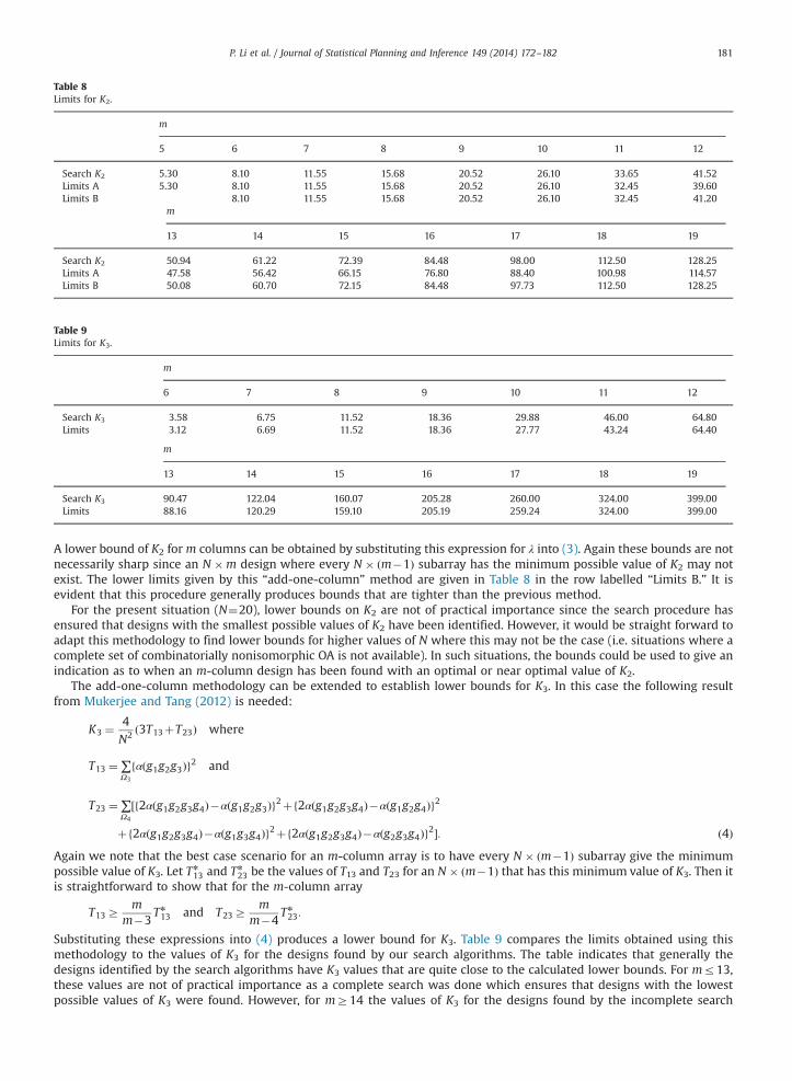
Table 8Limits for K2.

m

5 6 7 8 9 10 11 12

Search K2 5.30 8.10 11.55 15.68 20.52 26.10 33.65 41.52Limits A 5.30 8.10 11.55 15.68 20.52 26.10 32.45 39.60Limits B 8.10 11.55 15.68 20.52 26.10 32.45 41.20

m

13 14 15 16 17 18 19

Search K2 50.94 61.22 72.39 84.48 98.00 112.50 128.25Limits A 47.58 56.42 66.15 76.80 88.40 100.98 114.57Limits B 50.08 60.70 72.15 84.48 97.73 112.50 128.25

Table 9Limits for K3.

m

6 7 8 9 10 11 12

Search K3 3.58 6.75 11.52 18.36 29.88 46.00 64.80Limits 3.12 6.69 11.52 18.36 27.77 43.24 64.40

m

13 14 15 16 17 18 19

Search K3 90.47 122.04 160.07 205.28 260.00 324.00 399.00Limits 88.16 120.29 159.10 205.19 259.24 324.00 399.00

P. Li et al. / Journal of Statistical Planning and Inference 149 (2014) 172–182 181

A lower bound of K2 for m columns can be obtained by substituting this expression for λ into (3). Again these bounds are notnecessarily sharp since an N �m design where every N � ðm�1Þ subarray has the minimum possible value of K2 may notexist. The lower limits given by this “add-one-column” method are given in Table 8 in the row labelled “Limits B.” It isevident that this procedure generally produces bounds that are tighter than the previous method.

For the present situation (N¼20), lower bounds on K2 are not of practical importance since the search procedure hasensured that designs with the smallest possible values of K2 have been identified. However, it would be straight forward toadapt this methodology to find lower bounds for higher values of N where this may not be the case (i.e. situations where acomplete set of combinatorially nonisomorphic OA is not available). In such situations, the bounds could be used to give anindication as to when an m-column design has been found with an optimal or near optimal value of K2.

The add-one-column methodology can be extended to establish lower bounds for K3. In this case the following resultfrom Mukerjee and Tang (2012) is needed:

K3 ¼4

N2 3T13þT23ð Þ where

T13 ¼∑Ω3

fαðg1g2g3Þg2 and

T23 ¼∑Ω4

½f2αðg1g2g3g4Þ�αðg1g2g3Þg2þf2αðg1g2g3g4Þ�αðg1g2g4Þg2

þf2αðg1g2g3g4Þ�αðg1g3g4Þg2þf2αðg1g2g3g4Þ�αðg2g3g4Þg2�: ð4ÞAgain we note that the best case scenario for an m-column array is to have every N � ðm�1Þ subarray give the minimumpossible value of K3. Let T

n

13 and Tn

23 be the values of T13 and T23 for an N � ðm�1Þ that has this minimum value of K3. Then itis straightforward to show that for the m-column array

T13Zm

m�3Tn

13 and T23Zm

m�4Tn

23:

Substituting these expressions into (4) produces a lower bound for K3. Table 9 compares the limits obtained using thismethodology to the values of K3 for the designs found by our search algorithms. The table indicates that generally thedesigns identified by the search algorithms have K3 values that are quite close to the calculated lower bounds. For mr13,these values are not of practical importance as a complete search was done which ensures that designs with the lowestpossible values of K3 were found. However, for mZ14 the values of K3 for the designs found by the incomplete search

P. Li et al. / Journal of Statistical Planning and Inference 149 (2014) 172–182182

algorithm are all reasonably close to the calculated bounds. Keeping in mind that the bounds are not necessarily sharp, thisprovides some additional evidence that the incomplete search algorithm has performed well.

7. Concluding remarks

In this paper, we have provided a catalogue of baseline optimal designs for experiments of 20 runs for m¼5–19 factors –baseline optimal designs for smaller run sizes are provided by Mukerjee and Tang (2012). A complete search algorithm wasemployed to find the minimum K-aberration designs for mr13. For mZ14, we developed a search algorithm anddemonstrate that it is very effective at finding designs that are near optimal in terms of K-aberration. Clearly, this algorithmcan be easily extended to search for designs of larger run size. We have also developed methodology for establishing lowerbounds on K2 and K3 which can also be easily extended for designs of more than 20 runs.

Acknowledgements

Boxin Tang's research is supported by the Natural Sciences and Engineering Research Council of Canada. The authorswould like to thank two referees for their useful comments.

References

Aarts, E., Lenstra, J.K., 2003. Local Search in Combinatorial Optimization. Princeton University Press, New Jersey.Banerjee, T., Mukerjee, R., 2008. Optimal factorial designs for cDNA microarray experiments. Ann. Appl. Statist. 2, 366–385.Box, G.E.P., Hunter, K.P., 1961. The 2k�p fractional factorial designs. Technometrics 3, 311–351.Kerr, K.F., 2006. Efficient 2k factorial designs for blocks of size 2 with microarray applications. J. Qual. Technol. 38, 309–318.Li, P., 2011. Algorithmic Search of Baseline Minimum Aberration Designs (M.Sc. thesis). Department of Statistics and Actuarial Science, Simon Fraser

University, Burnaby, British Columbia, Canada.Mukerjee, R., Tang, B., 2012. Optimal fractions of two-level factorials under a baseline parameterization. Biometrika 99, 71–84.Mukerjee, R., Wu, C.F.J., 2006. A Modern Theory of Factorial Designs. Springer, New York.Wu, C.F.J., Hamada, M.S., 2009. Experiments: Planning, Analysis and Optimization, 2nd ed. Wiley, Hoboken, New Jersey.Xu, H., Phoa, F.K.H., Wong, W.K., 2009. Recent developments in nonregular fractional factorial designs. Statist. Surveys 3, 18–46.