Submitted to:Infinity 2013

c© O. MalerThis work is licensed under theCreative Commons Attribution License.

Algorithmic Verification of Continuousand Hybrid Systems

Oded MalerCNRS-VERIMAG,

University of GrenobleFrance

We provide a tutorial introduction to reachability computation, a class of computational techniquesthat exports verification technology toward continuous and hybrid systems. For open under-determinedsystems, this technique can sometimes replace an infinite number of simulations.

1 Introduction

The goal of this article is to introduce the fundamentals of algorithmic verification of continuous dy-namical systems defined by differential equations and of hybrid dynamical systems defined by hybridautomata which are dynamical systems that can switch between several modes of continuous dynamics.There are two types of audience that I have in mind. The first is verification-aware computer scientistswho know finite-state automata and their algorithmic analysis. For this audience, the conceptual schemeunderlying the presented algorithms will be easy to grasp as it is mainly inspired by symbolic model-checking of non-deterministic automata. Putting aside dense time and differential equations, dynamicalsystems can be viewed by this audience as a kind of infinite-state reactive program defined over the so-called real numbers. For this reason, I will switch from continuous to discrete-time discourse quite earlyin the presentation.

The other type of audience is people coming from control or other types of engineering and appliedmathematics. These are relatively well versed in the concrete mathematics of continuous systems andshould first be persuaded that the verification question is interesting, despite the fact that airplanes canfly (and theoretical papers can be written) without it. In my attempts to accommodate these two typesof audience, I have written some explanation that will look trivial to some but this cannot be avoidedwhile trying to do genuine inter-disciplinary research1 (see also [65] for an attempt to unify discreteand continuous systems and [69] for some historical reflections). My intention is to provide a syntheticintroduction to the topic rather than an exhaustive survey, hence the paper is strongly biased towardtechniques closer to my own research. In particular, I will not deal with decidability results for hybridsystems with simplified dynamics and not with deductive verification methods that use invariants, barriersand Lyapunov functions. I sincerely apologize to those who will not find citations of their relevant work.

The rest of the paper is organized as follows. Section 2 describes the problem and situates it incontext. Section 3 gives the basic definitions of reachability notions used throughout the paper. Section 4presents the principles of set-based computation as well as basic issues related to the computationaltreatment of sets in general and convex polytopes in particular. Section 5 is devoted to reachabilitytechniques for linear and affine dynamical systems in both discrete and continuous time, the domain

1The need to impress the members of one’s own community is perhaps the main reason for the sterility of many attempts todo inter-disciplinary research.

2 Algorithmic verification of continuous and hybrid systems

where a lot of progress has been made in recent years. The extension of these techniques to hybrid andnon-linear systems, an active area of research, is discussed in Section 6. I conclude with some discussionof related work and new research directions.

2 The Problem

This paper is concerned with the following problem that we define first in a quasi-formal manner:Consider a continuous dynamical system with input defined over some bounded state space X and

governed by a differential equation of the form2

x = f (x,v)

where v[t] ranges, for every t, over some pre-specified bounded set V of admissible input values. Givena set X0 ⊂ X, compute all the states visited by trajectories of the system starting from any x0 ∈ X0.

The significance of this question to control is the following: consider a controller that has been de-signed and connected to its plant and which is subject to external disturbances modeled by v. Computingthe reachable set allows one to verify that all the behaviors of the closed-loop system stay within a desiredrange of operation and do not reach a forbidden region of the state space. Proving such properties forsystems subject to uncontrolled interaction with the external environment is the main issue in verificationof programs and digital hardware from which this question originates. In verification you have a largeautomaton with inputs that represent non-deterministic (non-controllable) effects such as behaviors ofusers and interactions with other systems and you would like to know whether there is an input sequencethat drives the automaton into a forbidden state.

Before going further, let me try to situate this problem in the larger control context. After all, controltheory and practice have already existed for many years without asking this question nor trying to answerit. This question distinguishes itself from traditional control questions in the following respects:

1. It is essentially a verification rather than a synthesis question, that is, the controller is assumed toexist already. However, it has been demonstrated that variants of reachability computation can beused for synthesizing switching controllers for timed [14, 8, 21] and hybrid [9] systems.

2. External disturbances are modeled explicitly as a set of admissible inputs, which is not the casefor certain control formulations.3 These disturbances are modeled in a set-theoretic rather thanstochastic manner, that is, only the set of possible disturbances is specified without any probabilityinduced over it. This makes the system in question look like a system defined by differentialinclusions [16] which are the continuous analog of non-deterministic automata: if you projectaway the input you move from x = f (x,v) to x ∈ F(x). Adding probabilities the the inputs willyield a kind of a stochastic differential equation [15].

3. The information obtained from reachability computation covers also the transient behavior of thesystem in question, and not only its steady-state behavior. This property makes the approachparticularly attractive for the analysis of hybrid (discrete-continuous, numerical-logical) systemswhere the applicability of analytic methods is rather limited. Such hybrid models can express,for example, deviation from idealized linear models due to constraints and saturation as well asother switching phenomena such as thermostat-controlled heating or gear shifting, see [66] for

2We use the physicists’ notation where x indicates dx/dt. It is amusing to note that the idea of having a dedicated notationfor the special variable called Time, is not unique to Temporal Logic.

3See [68] for a short discussion of this intriguing fact.

O. Maler 3

a lightweight introduction to hybrid systems and more elaborate accounts in books, surveys andlecture notes such as [74, 17, 64, 48, 61, 80, 76, 30, 20, 4].

4. The notion of to compute has a more effective flavor, that is, to develop algorithms that produce arepresentation of the set of reachable states (or an approximation of it) which is computationallyusable, for example, it can be checked for intersection with a bad set of states.

Perhaps the most intuitive explanation of what is going on in reachability computation (and verifica-tion in general) can be given in terms of numerical simulation, which is by far the most commonly-usedapproach for validating complex systems. Each individual simulation consists of picking one initial con-dition and one input stimulus (random, periodic, step, etc.), producing the corresponding trajectory usingnumerical integration and observing whether this trajectory behaves properly. Ideally, to be on the safeside, one would like to repeat this procedure with all possible disturbances which are uncountably many.Reachability computation achieves the same effect as exhaustive simulation by exploring the state spacein a “breadth-first” manner: rather than running each individual simulation to completion and then start-ing a new one, we compute at each time step all the states reachable by all possible one-step inputs fromstates reachable in the previous step (see [67] for a more elaborate development of this observation and[70] for a more general discussion of under-determined systems and their simulation). This set-basedsimulation is, of course, much more costly than the simulation of an individual trajectory but it providesmore confidence in the correctness of the system than a small number of individual simulations would.The paper is focused on one popular approach to reachability computation based on discretizing timeand performing a kind of set-based numerical integration. Alternative approaches are mentioned brieflyat the end.

3 Preliminaries

We assume a time domain T =R+ and a state space X ⊆Rn. A trajectory is a measurable partial functionξ : T → X defined over all T (infinite trajectory) or over an interval [0, t]⊂ T (a finite trajectory). We usethe notation T (X) for all such trajectories and |ξ |= t to denote the length (duration) of finite signals. Weconsider an input space V ⊆Rm and likewise use T (V ) to denote input signals ζ : T →V . A continuousdynamical system S = (X ,V, f ) is a system defined by the differential equation

x = f (x,v). (1)

We say that ξ is the response of f to ζ from x if ξ is the solution of (1) for initial condition x and v(.) = ζ .We denote this fact by ξ = fx(ζ ) and also as

xζ/ξ−→ x′

when |ζ | = t and ξ [t] = x′. In this case we say that x′ is reachable from x by ζ within t time and writethis as

R(x,ζ , t) = x′.

This notion speaks of one initial state, one input signal and one time instant and its generalization for aset X0 of initial states, for all time instants in an interval I = [0, t] and for all admissible input signals inT (V ) yields the definition of the reachable set:

RI(X0) =⋃

x∈X0

⋃t∈I

⋃ζ∈T (V )

R(x,ζ , t).

4 Algorithmic verification of continuous and hybrid systems

x0x0

Figure 1: Trajectories induced by input signals from x0 and the set of reachable states.

Figure 1 illustrates the induced trajectories and the reachable states for the case where X0 = x0. We willuse the same RI notation also when I is not an interval but an arbitrary time set. For example R[1..r](X0)can denote either the states reachable from X0 by a continuous-time systems at discrete time instants, orstates reachable by a discrete-time system during the first r steps.

Note that our introductory remark equating the relation between simulation and reachability compu-tation to the relation between breadth-first and depth-first exploration of the space of trajectories corre-sponds to the commutativity of union:

⋃t∈I

⋃ζ∈T (V )

R(x,ζ , t) =⋃

ζ∈T (V )

⋃t∈I

R(x,ζ , t).

4 Principles

In what follows we lay down the principles of one of the most popular approaches for computing reach-able sets which is essentially a set-based extension of numerical integration.

4.1 The Abstract Algorithm

The semigroup property of dynamical systems, discrete and continuous alike, allows one to computetrajectories incrementally. The reachability operator also admits this property which is expressed as:

R[0,t1+t2](X0) = R[0,t2](R[0,t1](X0)).

Hence, the computation of RI(X0) for an interval I = [0,L] can be carried out by picking a time step rand executing the following algorithm:

Algorithm 1 (Abstract Incremental Reachability)

O. Maler 5

Input: A set X0 ⊂ XOutput: Q = R[0,L](X0)

P := Q := X0repeat i = 1,2 . . .P := R[0,r](P)Q := Q∪P

until i = L/r

Remark: When interested in reachability for unbounded horizon, the termination condition i = L/rshould be replaced by P ⊆ Q, that is, the newly-computed reachable states are included in the set ofstates already computed. With this condition the algorithm is not guaranteed to terminate. Throughoutmost of this article we focus on reachability problems for a bounded time horizon.

4.2 Representation of Sets

The most urgent thing needed in order to convert the above scheme into a working algorithm is to choosea class of subsets of X that can be represented in the computer and be subject to the operations appearingin the algorithm. This is a very important issue, studied extensively (but often in low dimension) incomputer graphics and computational geometry, but less so in the context of dynamical systems andcontrol, hence we elaborate on it a bit bringing in, at least informally, some notions related to effectivecomputation.

Mathematically speaking, subsets of Rn are defined as those points that satisfy some predicate. Suchpredicates are syntactic descriptions of the set and the points that satisfy them are the semantic objectswe are interested in. The syntax of mathematics allows one to define weird types of sets which arenot subject to any useful computation, for example, the set of irrational numbers. In order to computewe need to restrict ourselves to (syntactically characterized) classes of sets that satisfy the followingproperties:

1. Every set P in the class C admits a finite representation.

2. Given a representation of a set P ∈ C and a point x, it is possible to check in a finite number ofsteps whether x ∈ P.

3. For every operation on sets that we would like to perform and every P1,P2 ∈ C we have P1 P2 ∈C . Moreover, given representations of P1 and P2 it should be possible to compute a representationof P1 P2.

The latter requirement is often referred to as C being effectively closed under . This requirement willlater be relaxed into requiring that C contains a reasonable approximation of P1 P2. To illustrate thesenotions, let us consider first a negative example of a class of sets admitting a finite representation but notsatisfying requirements 2 and 3 above. The reachable set of a linear system x = Ax can be “computed”and represented by a finite formula of the form

RI(X0) = x : ∃x0 ∈ X0 ∃t ∈ I x = x0eAt,

however this representation is not very useful because, in the general case, checking the membership ofa point x in this set amounts to solving the reachability problem itself! The same holds for checking

6 Algorithmic verification of continuous and hybrid systems

x1

x2

y2

x

x

y

y1

x2

y2

x1

y

y1

z2

z1

z2

z1

z

z

Figure 2: Intersecting two rectangles represented as 〈x,x〉 and 〈y,y〉 to obtain a rectangle representedas 〈z,z〉. The computation is done by letting z1 = max(x1,y1), z2 = max(x2,y2), z1 = min(x1,y1) andz2 = min(x2,y2).

whether this set intersects another set. On the other hand, a set defined by a quantifier-free formula ofthe form

x : g(x)≥ 0,

where g is some computable function, admits in principle a membership check for every x: just evaluateg(x) and compare with 0.

As a further illustration consider one of the simplest classes of sets, hyper-rectangles with axes-parallel edges and rational endpoints. Such a hyper-rectangle can be represented by its leftmost andrightmost corners x = (x1, . . . ,xn) and x = (x1, . . . ,xn). The set is defined as all points x = (x1, . . . ,xn)satisfying

n∧i=1

xi ≤ xi ≤ xi,

a condition which is easy to check. As for operations, this class is effectively closed under translation(just add the displacement vector to the endpoints), dilation (multiply the endpoints by a constant) but notunder rotation. As for Boolean set-theoretic operations, it is not hard to see that rectangles are effectivelyclosed under intersection by component-wise max of their leftmost corners and component-wise min oftheir rightmost corners, see Figure 2. However they are not closed under union and complementation.This is, in fact, a general phenomenon that we encounter in reachability computations, where the basicsets that we work with are convex, but their union is not and hence the reachable sets computed byconcrete realizations of Algorithm 1 will be stored as unions (lists) of convex sets (the recent algorithmof [38] is an exception).

As mentioned earlier, sets can be defined using combinations of inequalities and, not surprisingly,linear inequalities play a prominent role in the representation of some of the most popular classes ofsets. We will mostly use convex polytopes, bounded polyhedra definable as conjunctions of linear in-equalities. Let us mention, though, that Boolean combinations of polynomial inequalities define thesemi-algebraic sets, which admit some interesting mathematical and computational results. Their algo-rithmics is, however, much more complex than that of polyhedral sets. The only class of sets definableby nonlinear inequalities for which relatively-efficient algorithms have been developed is the class ofellipsoids, convex sets defined as deformations of a unit circle by a (symmetric and positive definite)

O. Maler 7

linear transformation [54]. Ellipsoids can be finitely represented by their center and the transformationmatrix and like polytopes, they are closed under linear transformations, a fact that facilitates their use inreachability computation for linear systems. Ellipsoids differ from polytopes by not being closed underintersection but such intersections can be approximated to some extent.

4.3 Convex Polytopes

In the following we list some facts concerning convex polytopes. These objects, which underlie otherdomains such as linear programming, admit a very rich theory of which we only scratch the surface.Readers interested in more details and precision may consult textbooks such as [75, 82].

A linear inequality is an inequality of the form a · x ≤ b with a being an n-dimensional vector. Theset of all points satisfying a linear inequality is called a halfspace. Note that the relationship betweenhalfspaces and linear inequalities is not one-to-one because any inequality of the form ca · x ≤ cb, withc positive, will represent the same set. However using some conventions one can establish a uniquerepresentation for each halfspace. A convex polyhedron is an intersection of finitely many halfspaces. Aconvex polytope is a bounded convex polyhedron. A convex combination of a set x1, . . . ,xl of pointsis any x = λ1x1 + · · ·+λlxl such that

l∧i=1

λi ≥ 0∧l

∑i=1

λi = 1.

The convex hull of a set P of points, denoted by P = conv(P), is the set of all convex combinations of itselements. Convex polytopes admit two types of canonical representations:

1. Vertices: each convex polytope P admits a finite minimal set P such that P = conv(P). The ele-ments of P are called the vertices of P.

2. Inequalities: a convex polytope P admits a minimal set H = H1, . . . ,Hk of halfspaces such thatP =

⋂ki=1 H i. This set is represented syntactically as a conjunction of inequalities

k∧i=1

ai · x≤ bi.

Some operations are easier to perform on one representation and some on the other. Testing membershipx ∈ P is easier using inequalities (just evaluation) while using vertices representation, one needs to solvea system of linear equations to find the λ ’s. To check whether P1∩P2 6= /0 one can first combine syntac-tically the inequalities of P1 and P2 but in order to check emptiness, these inequalities should be broughtinto a canonical form. On the other hand, conv(P) is always non-empty for any non-empty P. Various(worst-case exponential) algorithms convert polytopes from one representation to the other.

The most interesting property of convex polytopes, which is also shared by ellipsoids, is the fact thatthey are closed under linear operators, that is, for a matrix A, if P is a convex polytope (resp. ellipsoid)so is the set

AP = Ax : x ∈ P

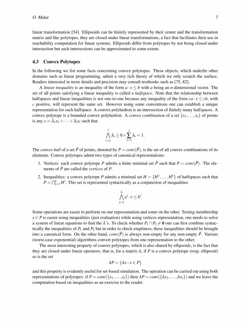
and this property is evidently useful for set-based simulation. The operation can be carried out using bothrepresentations of polytopes: if P = conv(x1, . . . ,xl) then AP = conv(Ax1, . . . ,Axl) and we leave thecomputation based on inequalities as an exercise to the reader.

8 Algorithmic verification of continuous and hybrid systems

x′4 = Ax4

x′6 = Ax6x′1 = Ax1

AP

x′3 = Ax3

x′2 = Ax2

x′5 = Ax5

x1

x2

x5

x6

x3

Px4

Figure 3: Computing AP from P by applying A to the vertices.

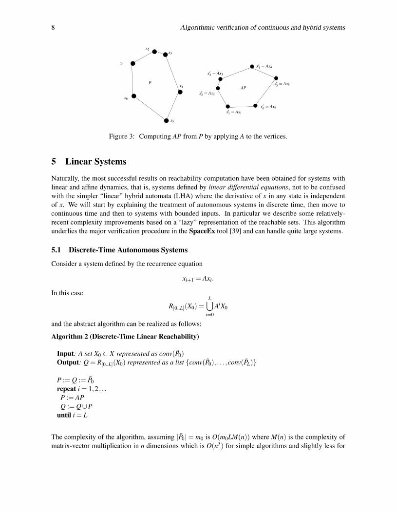
5 Linear Systems

Naturally, the most successful results on reachability computation have been obtained for systems withlinear and affine dynamics, that is, systems defined by linear differential equations, not to be confusedwith the simpler “linear” hybrid automata (LHA) where the derivative of x in any state is independentof x. We will start by explaining the treatment of autonomous systems in discrete time, then move tocontinuous time and then to systems with bounded inputs. In particular we describe some relatively-recent complexity improvements based on a “lazy” representation of the reachable sets. This algorithmunderlies the major verification procedure in the SpaceEx tool [39] and can handle quite large systems.

5.1 Discrete-Time Autonomous Systems

Consider a system defined by the recurrence equation

xi+1 = Axi.

In this case

R[0..L](X0) =L⋃

i=0

AiX0

and the abstract algorithm can be realized as follows:

Algorithm 2 (Discrete-Time Linear Reachability)

Input: A set X0 ⊂ X represented as conv(P0)Output: Q = R[0..L](X0) represented as a list conv(P0), . . . ,conv(PL)

P := Q := P0repeat i = 1,2 . . .

P := APQ := Q∪P

until i = L

The complexity of the algorithm, assuming |P0| = m0 is O(m0LM(n)) where M(n) is the complexity ofmatrix-vector multiplication in n dimensions which is O(n3) for simple algorithms and slightly less for

O. Maler 9

fancier ones. As noted, this algorithm can be applied to other representations of polytopes, to ellipsoidsand any other class of sets closed under linear transformations. If the purpose of reachability is todetect intersection with a set B of bad states we can weaken the loop termination condition into (i =L)∨ (P∩B 6= /0) where the intersection test is done by transforming P into an inequalities representation.If we consider unbounded horizon and want to detect termination we need to check whether the newly-computed P is included in Q which can be done by “sifting” P through all the polytopes in Q andchecking whether it goes out empty. This is not a simple operation but can be done. In any case, there isno guarantee that this condition will ever become true.

5.2 Continuous-Time Autonomous Systems

The approach just described can be adapted to continuous-time systems of the form

x = Ax

as follows. First it is well known that by choosing a time step r and computing the corresponding matrixexponential A′ = eAr we obtain a discrete-time system

xi+1 = A′xi

which approximates the original system in the sense that for every i, xi of the discrete-time system is closeto x[ir] of the continuous-time system. The quality of the approximation can be indefinitely improved bytaking smaller r. We then use the discrete time reachability operator to compute P′ = Rr(P) = A′P, thatis, the successors of P at time r and can use one out of several techniques to compute an approximationof R[0,r](P) from P and P′:

5.2.1 Make r Small

This approach, used implicitly by [53], just makes r small enough so that subsequent sets overlap eachother and the difference between their unions and the continuous-time reachable set vanishes.

5.2.2 Bloating

Let P and P′ be represented by the sets of vertices P and P′ respectively. The set P = conv(P∪ P′) is agood approximation of R[0,r](P) but since in general, we would like to obtain an over-approximation (sothat if the computed reachable sets does not intersect with the bad set, we are sure that the actual set doesnot either) we can bloat this set to ensure that it is an outer approximation of R[0,r](P).

This can be done, for example, by pushing the facets of P outward by a constant derived from theTaylor approximation of the curve [12]. To this end we need first to transform P into an inequalitiesrepresentation. An alternative approach [24] is to find this over-approximation via an optimization prob-lem. Note that for autonomous systems we can modify Algorithm 1 by replacing the initialization byP := Q := R[0,r](X0) and the iteration by P := R[r,r](P), that is, the successors after exactly r time units.This way the over-approximation is done only once for conv(P0∪ P1) and then A is applied successivelyto this set [58].

10 Algorithmic verification of continuous and hybrid systems

5.2.3 Adding an Error Term

The last approach that we mention is particularly interesting because it can be used, as we shall see later,also for non-autonomous systems as well as nonlinear ones. Let Y and Y ′ be two subsets of Rn. TheirMinkowski sum is defined as

Y ⊕Y ′ = y+ y′ : y ∈ Y ∧ y′ ∈ Y ′.

The maximal distance between the sets Rr(P) and R[0,r](P) can be estimated globally. Then, one can fixan “error ball” E (could be a polytope for that matter) of that radius and over-approximate R[0,r](P) asAP⊕E. Since this computation is equivalent to computing the reachable set of the discrete time systemxi+1 = A′xi+e with e∈ E, we can use the techniques for systems with input described in the next section.

5.3 Discrete-Time Systems with Input

We can now move, at last, to open systems of the form

xi+1 = Axi +Bvi

where v ranges over a bounded convex set V . The one-step successor of a set P is defined as

P′ = Ax+Bv : x ∈ P,v ∈V= AP⊕BV.

Unlike linear operations that preserve the number of vertices of a convex polytope, the Minkowski sumincreases their number and its successive application may prohibitively increase the representation size.Consequently, methods for reachability under disturbances need some compromise between exact com-putation that leads to explosion, and approximations which keep the representation size small but mayaccumulate errors to the point of becoming useless, a phenomenon also known in numerical analysis asthe “wrapping effect” [50, 51]. We illustrate this tradeoff using three approaches.

5.3.1 Using Vertices

Assume both P and V are convex polytopes represented by their vertices, P = conv(P) and V = conv(V ).Then it is not hard to see that

AP⊕BV = conv(Ax+Bv : x ∈ P,v ∈ V).

Hence, applying the affine transformation to all combinations of vertices in P× V we obtain all thecandidates for vertices of P′ (see Figure 4). Of course, not all of these are actual vertices of P′ but thereis no known efficient procedure to detect which are and which are not. Moreover, it may turn out thatthe number of actual vertices indeed grows in a super-linear way. Neglecting the elimination of fictitiousvertices and keeping all these points as a representation of P′ will lead to |P| · |V |k vertices after k steps,a completely unacceptable situation.

5.3.2 Pushing Facets

This approach over-approximates the reachable set while keeping its complexity more or less fixed. As-sume P to be represented in (or converted into) inequality representation. For each supporting halfspaceH i defined by ai ·x≤ bi, let vi ∈V be the disturbance vector which pushes H i in the “outermost” way, thatis, the one which maximizes the product v ·ai with the normal to H i. In the discrete time setting described

O. Maler 11

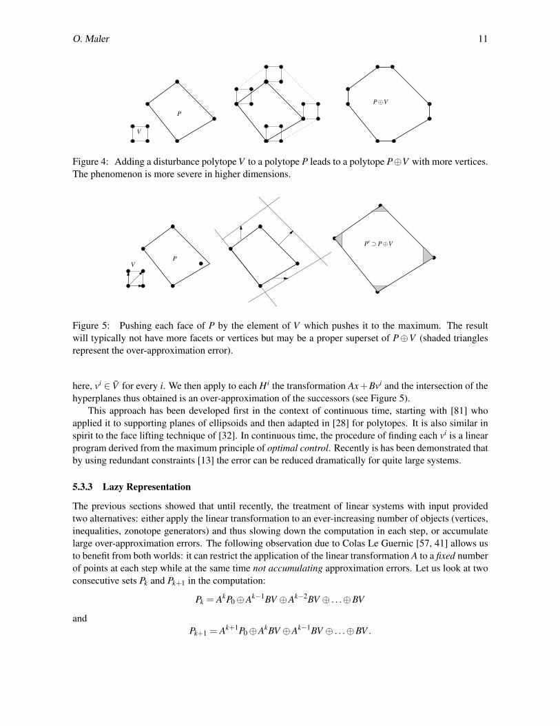
P⊕V

P

V

Figure 4: Adding a disturbance polytope V to a polytope P leads to a polytope P⊕V with more vertices.The phenomenon is more severe in higher dimensions.

P′ ⊃ P⊕V

PV

Figure 5: Pushing each face of P by the element of V which pushes it to the maximum. The resultwill typically not have more facets or vertices but may be a proper superset of P⊕V (shaded trianglesrepresent the over-approximation error).

here, vi ∈ V for every i. We then apply to each H i the transformation Ax+Bvi and the intersection of thehyperplanes thus obtained is an over-approximation of the successors (see Figure 5).

This approach has been developed first in the context of continuous time, starting with [81] whoapplied it to supporting planes of ellipsoids and then adapted in [28] for polytopes. It is also similar inspirit to the face lifting technique of [32]. In continuous time, the procedure of finding each vi is a linearprogram derived from the maximum principle of optimal control. Recently is has been demonstrated thatby using redundant constraints [13] the error can be reduced dramatically for quite large systems.

5.3.3 Lazy Representation

The previous sections showed that until recently, the treatment of linear systems with input providedtwo alternatives: either apply the linear transformation to an ever-increasing number of objects (vertices,inequalities, zonotope generators) and thus slowing down the computation in each step, or accumulatelarge over-approximation errors. The following observation due to Colas Le Guernic [57, 41] allows usto benefit from both worlds: it can restrict the application of the linear transformation A to a fixed numberof points at each step while at the same time not accumulating approximation errors. Let us look at twoconsecutive sets Pk and Pk+1 in the computation:

Pk = AkP0⊕Ak−1BV ⊕Ak−2BV ⊕ . . .⊕BV

andPk+1 = Ak+1P0⊕AkBV ⊕Ak−1BV ⊕ . . .⊕BV .

12 Algorithmic verification of continuous and hybrid systems

As one can see, these two sets “share” a lot of common terms that need not be recomputed (and thisholds also for continuous-time and variable time-steps). And indeed, the algorithm described in [41]computes the sequence P0, . . . ,Pk in O(k(m0 +m)M(n)) time. From this symbolic/lazy representation ofPi, one can produce an approximating polytope with any desired precision, but this object is not used tocompute Pi+1 and hence the wrapping effect is avoided.

A first prototype implementation of that algorithm could compute the reachable set after 1000 stepsfor linear systems with 200 state variables within 2 minutes. This algorithm was first discovered forzonotopes (a class of centrally symmetric polytopes closed under Minkowski sum proposed for reacha-bility in [40]) but was later adapted to arbitrary convex sets represented by support functions [60, 58]. Are-engineered version of the algorithm has been implemented into the SpaceEx tool [39]. Although onemight get the impression that the reachability problem for linear systems can be considered as solved,the development of SpaceEx under the direction of Goran Frehse has confirmed once more that a lotof work is needed in order to transform bright ideas into a working tool that can robustly handle largenon-trivial systems occurring in practice.4

6 Hybrid and Nonlinear Systems

Being able to handle quite large linear systems, a major challenge is to extend reachability to richerclasses of systems admitting hybrid or nonlinear dynamics.

6.1 Hybrid systems

The analysis of hybrid systems was the major motivation for developing reachability algorithms becauseunlike analytical methods, these algorithms can be easily adapted to handle discrete transitions and modeswitching. Figure 6 shows a very simple hybrid automaton with two states, each with its own lineardynamics (using another terminology we have here a piecewise-linear or piecewise-affine dynamicalsystem). An (extended) state of a hybrid system is a pair (s,x) ∈ S×X where s is the discrete state(mode). A transitions from state si to state s j may occur when the condition Gi j(x) (the transition guard)is satisfied by the current value of x. Such conditions are typically comparisons of state variables withthresholds or more generally linear inequalities. Moreover, while staying at discrete state s, the value of xshould satisfy additional constraints, known as state invariants.5 Like timed automata, hybrid automatacan exhibit dense non-determinism in parts of the state-space where both a transition guard and a stateinvariant hold. The runs/trajectories of such an automaton are of the form

(s1,x[0])t1−→ (s1,x[t1])−→ (s2,x[t1])

t2−→ (s2,x[t1 + t2])−→ ·· · ,

that is, an interleaving of continuous trajectories and discrete transitions taken at extended states whereguards are satisfied. The adaptation of linear reachability computation so as to compute the reachablesubset of S×X follows the procedure proposed already in [5] for simpler dynamics and implementedin the HyTech tool [45]. It goes like this: first, continuous reachability is applied using the dynamicsA1 of s1, while respecting the state invariant I1. Then the set of reachable states is intersected withthe (semantics of the) transition guard G12. The outcome serves as an initial set of states in s2 wherecontinuous linear reachability with A2 and I2 is applied and so on.

4Readers are encouraged to download SpaceEx at http://spaceex.imag.fr/ to obtain a first hand experience inreachability computation.

5The full hybrid automaton model may also associate transitions with reset maps which are transformations (jumps) appliedto x upon a transition.

O. Maler 13

x = A1x+ v

G12(x)

G21(x)

x = A2x+ v

s1 s2 I2I2

Figure 6: A simple hybrid system with two modes.

The real story is, of course, not that simple for the following reasons.

1. The intersection of the reachable states with the state invariant breaks the symbolic lazy repre-sentation as soon as some part of the reachable set leaves the invariant. Likewise, the change ofdynamics after the transition invalidates the update scheme of the lazy representation and the sethas to be over-approximated before doing intersection and reachability in the next state.

2. The dynamics might be “grazing” the transition guard, intersecting different parts of it at differenttime steps, thus spawning many subsequent computations. In fact, even a dynamics which pro-ceeds orthogonally toward a single transition guard may spawn many such computations becausewhen small time steps are used, many consecutive sets may have a non-empty intersection withthe guard. Consequently, techniques for hybrid reachability such as [59] tend to cluster these setstogether before conducting reachability in the next state thus increasing the over-approximationerror. This error can now be controlled using the techniques of [38].

3. Even in the absence of these phenomena, when there are several transitions outgoing from a statewe may end up with an exponentially growing number of runs to explore.

All these are problems, some tedious and some glorious, that need to be resolved if we want to providea robustly working tool.

6.2 Nonlinear Systems

Many challenging problems in numerous engineering and scientific domains boil down to exploringthe behaviors of nonlinear systems. The techniques described so far take advantage of the intimaterelationships between linearity and convexity, in particular the identity A · conv(P) = conv(AP). Fornonlinear functions such properties do not hold and new ideas are needed. I sketch briefly two approchesfor adapting reachability for such systems: one which is general and is based on linearizing the system atvarious parts of the state-space thus obtaining a piecewise-linear system (a hybrid automaton) to whichlinear reachability techniques are applied. Other techniques look for more sophisticated data-structuresand syntactical objects that can represent sets reached by specific classes of nonlinear systems such asthose defined by polynomial dynamics. Unlike linear systems, linear reachability is still in an exploratoryphase and it is too early to predict which of the techniques described below will survive.

6.2.1 Linearization/Hybridization

Consider a nonlinear system x = f (x) and a partition of its state space, for example into cubes (seeFigure 7). For each cube s one can compute a linear function As and an error polytope Vs such that forevery x∈ s, f (x)−Asx∈Vs and hence we have a conservative approximation f (x)∈Asx⊕Vs. We can nowbuild a hybrid automaton (a piecewise-affine dynamical system) whose states correspond to the cubes,and which makes transitions (mode switching) from s to s′ whenever x crosses the boundary betweenthem (see Figure 7). The automaton provides an over approximation of the nonlinear system in the sense

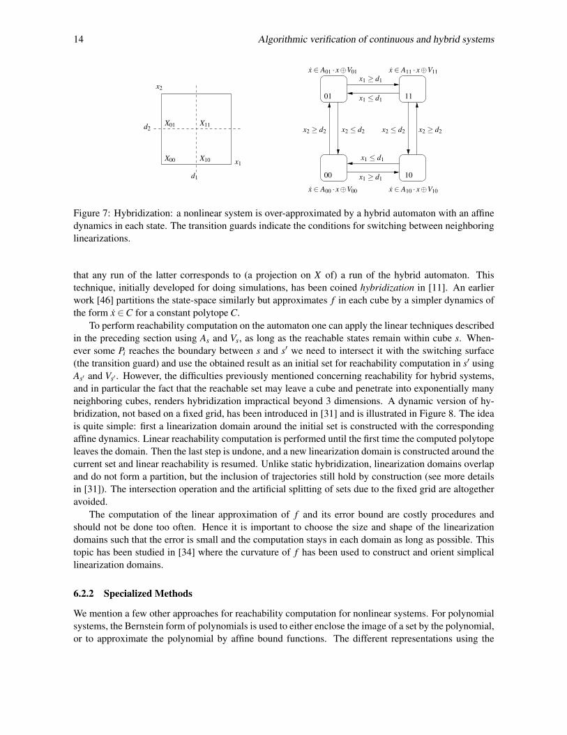
14 Algorithmic verification of continuous and hybrid systems

10

1101

00

x2 ≥ d2x2 ≤ d2x2 ≤ d2

x1 ≥ d1

x1 ≤ d1

x1 ≥ d1

x1 ≤ d1

x ∈ A00 · x⊕V00 x ∈ A10 · x⊕V10

x ∈ A01 · x⊕V01 x ∈ A11 · x⊕V11

x2 ≥ d2

d1

x1X10X00

X01 X11d2

x2

Figure 7: Hybridization: a nonlinear system is over-approximated by a hybrid automaton with an affinedynamics in each state. The transition guards indicate the conditions for switching between neighboringlinearizations.

that any run of the latter corresponds to (a projection on X of) a run of the hybrid automaton. Thistechnique, initially developed for doing simulations, has been coined hybridization in [11]. An earlierwork [46] partitions the state-space similarly but approximates f in each cube by a simpler dynamics ofthe form x ∈C for a constant polytope C.

To perform reachability computation on the automaton one can apply the linear techniques describedin the preceding section using As and Vs, as long as the reachable states remain within cube s. When-ever some Pi reaches the boundary between s and s′ we need to intersect it with the switching surface(the transition guard) and use the obtained result as an initial set for reachability computation in s′ usingAs′ and Vs′ . However, the difficulties previously mentioned concerning reachability for hybrid systems,and in particular the fact that the reachable set may leave a cube and penetrate into exponentially manyneighboring cubes, renders hybridization impractical beyond 3 dimensions. A dynamic version of hy-bridization, not based on a fixed grid, has been introduced in [31] and is illustrated in Figure 8. The ideais quite simple: first a linearization domain around the initial set is constructed with the correspondingaffine dynamics. Linear reachability computation is performed until the first time the computed polytopeleaves the domain. Then the last step is undone, and a new linearization domain is constructed around thecurrent set and linear reachability is resumed. Unlike static hybridization, linearization domains overlapand do not form a partition, but the inclusion of trajectories still hold by construction (see more detailsin [31]). The intersection operation and the artificial splitting of sets due to the fixed grid are altogetheravoided.

The computation of the linear approximation of f and its error bound are costly procedures andshould not be done too often. Hence it is important to choose the size and shape of the linearizationdomains such that the error is small and the computation stays in each domain as long as possible. Thistopic has been studied in [34] where the curvature of f has been used to construct and orient simplicallinearization domains.

6.2.2 Specialized Methods

We mention a few other approaches for reachability computation for nonlinear systems. For polynomialsystems, the Bernstein form of polynomials is used to either enclose the image of a set by the polynomial,or to approximate the polynomial by affine bound functions. The different representations using the

O. Maler 15

PiPi

P0P0

B

(a)

B

(b)

B′

Figure 8: Dynamic hybridization: (a) Computing in some box until intersection with the boundary; (b)Backtracking one step and computing in a new box.

Bernstein form include the Bezier simplices [29] and the Bernstein expansion [35, 77]. A nonlinearfunction can be over-approximated, based on its Taylor expansion, by a polynomial and an intervalwhich includes all the remainder values. Then, the integration of an ODE system can be done using thePicard operator with reachable sets are represented by boxes [22]. Similarly, in [2] non-linear functionsare approximated by linear differential inclusions with dynamical error estimated as the remainder of theTaylor expansion around the current set. As a set representation, “polynomial zonotopes” based on apolynomial rather than linear combination of generators are used.

We may conclude that the extension of reachability computation to nonlinear and hybrid systems isa challenging problem which is still waiting for several conceptual and algorithmic breakthroughs. Webelieve that the ability to perform reachability computation for nonlinear systems of non-trivial size canbe very useful not only for control systems but also for other application domains such as analog circuitsand systems biology. In biological models, uncertainty in parameters and environmental condition isa rule, not an exception, and set-based simulation, combined with other approaches for exploring theuncertainty space of under-determined dynamical systems can be very beneficial.

7 Related and Future Work

The idea of set-based numerical integration has several origins. In some sense it can be seen as relatedto those parts of numerical analysis, for example interval analysis [72, 47], that provide “robust” set-based results for numerical computation to compensate for numerical errors. This motivation is slightlydifferent from verification and control where the uncertainty is attributed to an external environment notto the internal computation. Set-based computations also underlie the abstract interpretation framework[27] for static analysis of software.

The idea of applying set-based computation to hybrid systems was among the first contributions ofthe verification community to hybrid systems research [5] and it has been implemented in the pioneeringHyTech tool [45]. However this idea was restricted to hybrid automata with very simple continuousdynamics (a constant derivative in each state) where trajectories can be computed without numericalintegration. To the best of our knowledge, the first explicit mention of combining numerical integrationwith approximate representation by polyhedra in the context of verification appeared in [43]. It wasrecently brought to my attention6 that an independent thread of reachability computation, quite similar inmotivation and techniques, has developed in the USSR starting from the early 70s [62]. More citationsfrom this school can be found in [63].

6G. Frehse, personal communication.

16 Algorithmic verification of continuous and hybrid systems

The polytope-based techniques described here were developed independently in [24, 23, 25] and in[12, 28]. Among other similar techniques that we have not described in detail, let us mention againthe extensive work on ellipsoids [54, 53, 19, 55] and another family of methods [71, 79] which usestechniques such as level sets, inspired by numerical solution of partial differential equations, to computeand represent the reachable states. Among the symbolic (non numerical) approaches to the problem let usmention [56] which computes an effective representation of the reachable states for a restricted class oflinear systems. Attempts to scale-up reachability techniques to higher dimensions using compositionalmethods that analyze an abstract approximate systems obtained by projections on subsets of the statevariables are described in [44] and [10].

The interpretation of V as the controller’s output rather than disturbance transforms the reachabil-ity problem into some open-loop variant of controller synthesis [67, 68]. Hence it is natural that theoptimization-based approach developed in [17] for synthesis, has also been applied to reachability com-putation [18]. On the other hand, reachability computation can be used to synthesize controllers in thespirit of dynamic programming, as has been demonstrated in [9] where a backward reachability operatorhas been used as part of an algorithm for synthesizing switching controllers.

Another class of methods, called simulation-based, for example [49, 42, 33, 37, 36, 1], attemptsto obtain the same effect as reachability computation by finitely many simulations, not necessarily ofextremal points as in the methods described in this paper. Such techniques may turn out to be superiorfor nonlinear systems whose dynamics does not preserve convexity and systems whose dynamics isexpressed by programs that do not always admit a clean mathematical model.

Alternative approaches to verify continuous and hybrid systems algorithmically attempt to approx-imate the system by a simpler one, typically a finite-state automaton7 [52, 7, 78]. This can be done bysimply partitioning the state space into cubes and defining transitions between adjacent cubes which areconnected by trajectories, or by more modern methods, inspired by program verification, such as pred-icate abstraction and counter-example based refinement [6, 26, 73]. It should be noted, however, thatfinite-state models based on space partitions suffer from the problem of false transitivity: the abstractsystem may have a run of the form s1→ s2→ s3 while the concrete one has no trajectory x1→ x2→ x3passing through these regions. As a result, the finite-state model will often have too many spuriousbehaviors to be useful for verification.

Finally let me mention some other issues not discussed so far:

• Disturbance models: implicit in reachability computation is the assumption that the only restrictionon the input signal is that it always remains in V . This means that it may oscillate in any frequencybetween the extremal values of V . Such a non realistic assumption may increase the reachable setand render the analysis too pessimistic. This effect can be reduced by composing the system witha bounded-variability non-deterministic model of the input generator but this will increase the sizeof the system. In fact, the technique of abstraction by projection [10] does the opposite: it projectsaway state-variables and converts them into bounded input variables. A more systematic study ofprecision/complexity tradeoffs could be useful here.

• Temporal properties: in our presentation we assumed implicitly that systems specifications aresimply invariance properties, a subclass of safety properties which are violated once a trajectoryreaches a forbidden state. It is, of course, possible to follow the usual procedure of taking a morecomplex temporal property, constructing its automaton and composing with the system model.This procedure will extend the discrete state-space of the system and will make the analysis harderby virtue of having more discrete transitions with the usual additional complications associated

7In fact, hybridization is another instance of this approach.

O. Maler 17

with detection of cycles in the reachability graph and extraction of concrete trajectories that realizethem.

• Adaptive algorithms: although we attempt to be as general as possible, it should be admitted thatdifferent systems lead to different behaviors of the reachability algorithm, even for linear systems.If we opt for general techniques that do not require a dedicated super-intelligent user, we needto make the algorithms more adaptive to their own behavior and automatically explore differentvalues of their parameters such as time steps, size and shapes of approximating polytopes, quickand approximate inclusion tests, different search strategies (for hybrid models) and more.

• Numerical aspects: the discourse in this paper treated real-valued computations as well-functioningblack boxes. In practice, certain systems can be more problematic in terms of numerical stabilityor operate in several time scales and this should be taken into account.

• Differential-algebraic equations: many dynamical systems that model physical phenomena obey-ing conservation laws are modeled using differential-algebraic equations with relational constraintsover variables and derivatives. In addition to the existing simulation technology for such systems,a specialized reachability theory should be developed, see for example [3].

• Discrete state explosion: the methods described here focus on scalability with respect to the di-mensionality of the continuous state-space and tacitly assume that the number of discrete modes isnot too large. This assumption can be wrong in at least two contexts: when discrete states are usedto encode different parts of a high dimensional state-space as in hybridization or in the verificationof complex control software when there is a relatively small number of continuous variables usedto model the environment of the software which has many states. The problem of combining thesymbolic representations for discrete and continuous spaces, for example BDDs and polytopes, isan unsolved problem already for the simplest case of timed automata.

• Finally, in terms of usability, the whole set-based point of view is currently not the natural one forpractitioners (this is true also for verification versus testing in the discrete case) and the extractionof individual trajectories that violate the requirements as well as input signals that induce themwill make reachability more acceptable as a powerful model debugging method.

Acknowledgments: This work benefitted from discussions with George Pappas, Bruce Krogh, CharlesRockland, Eugene Asarin, Thao Dang, Goran Frehse, Anoine Girard, Alexandre Donze and Colas LeGuernic.

References[1] Houssam Abbas, Georgios Fainekos, Sriram Sankaranarayanan, Franjo Ivancic & Aarti Gupta (2013): Prob-

abilistic temporal logic falsification of cyber-physical systems. ACM Transactions on Embedded ComputingSystems (TECS) 12(2s), p. 95.

[2] Matthias Althoff (2013): Reachability analysis of nonlinear systems using conservative polynomializationand non-convex sets. In: HSCC, ACM, pp. 173–182.

[3] Matthias Althoff & Bruce Krogh (2013): Reachability Analysis of Nonlinear Differential-Algebraic Systems.[4] Rajeev Alur (2011): Formal verification of hybrid systems. In: EMSOFT, pp. 273–278.[5] Rajeev Alur, Costas Courcoubetis, Nicolas Halbwachs, Thomas A. Henzinger, Pei-Hsin Ho, Xavier Nicollin,

Alfredo Olivero, Joseph Sifakis & Sergio Yovine (1995): The Algorithmic Analysis of Hybrid Sys-tems. Theoretical Computer Science 138(1), pp. 3–34. Available at http://dx.doi.org/10.1016/0304-3975(94)00202-T.

18 Algorithmic verification of continuous and hybrid systems

[6] Rajeev Alur, Thao Dang & Franjo Ivancic (2006): Counterexample-guided predicate abstraction of hybridsystems. Theoretical Computer Science 354(2), pp. 250–271. Available at http://dx.doi.org/10.1016/j.tcs.2005.11.026.

[7] Rajeev Alur, Thomas A Henzinger, Gerardo Lafferriere & George J Pappas (2000): Discrete abstractions ofhybrid systems. Proceedings of the IEEE 88(7), pp. 971–984.

[8] E Asarin, O Maler, A Pnueli & J Sifakis (1998): Controller synthesis for timed automata. Elsevier. Availableat http://www-verimag.imag.fr/PEOPLE/Oded.Maler/Papers/newsynth.pdf.

[9] Eugene Asarin, Olivier Bournez, Thao Dang, Oded Maler & Amir Pnueli (2000): Effective synthesis ofswitching controllers for linear systems. Proceedings of the IEEE 88(7), pp. 1011–1025. Available at http://www-verimag.imag.fr/˜maler/Papers/procieee.pdf.

[10] Eugene Asarin & Thao Dang (2004): Abstraction by Projection and Application to Multi-affine Systems. In:HSCC, LNCS 2993, Springer, pp. 32–47. Available at http://springerlink.metapress.com/openurl.asp?genre=article&issn=0302-9743&volume=2993&spage=32.

[11] Eugene Asarin, Thao Dang & Antoine Girard (2007): Hybridization methods for the analysis of nonlin-ear systems. Acta Informatica 43(7), pp. 451–476. Available at http://dx.doi.org/10.1007/s00236-006-0035-7.

[12] Eugene Asarin, Thao Dang, Oded Maler & Olivier Bournez (2000): Approximate Reachability Analysis ofPiecewise-Linear Dynamical Systems. In: HSCC, LNCS 1790, Springer, pp. 20–31. Available at http://link.springer.de/link/service/series/0558/bibs/1790/17900020.htm.

[13] Eugene Asarin, Thao Dang, Oded Maler & Romain Testylier (2010): Using Redundant Constraints forRefinement. In: ATVA, pp. 37–51. Available at http://www-verimag.imag.fr/˜maler/Papers/redundant.pdf.

[14] Eugene Asarin, Oded Maler & Amir Pnueli (1995): Symbolic Controller Synthesis for Discrete and TimedSystems. In: Hybrid Systems II, 999, Springer, pp. 1–20. Available at http://www-verimag.imag.fr/˜maler/Papers/symbolic.pdf.

[15] Karl J Astrom (1970): Introduction to stochastic control theory. Academic Press.

[16] Jean-Pierre Aubin & Arrigo Cellina (1984): Differential inclusions : set-valued maps and viability theory.Grundlehren der mathematischen Wissenschaften 264, Springer-Verlag.

[17] Alberto Bemporad & Manfred Morari (1999): Control of systems integrating logic, dynamics, and con-straints. Automatica 35(3), pp. 407–427.

[18] Alberto Bemporad, Fabio Danilo Torrisi & Manfred Morari (2000): Optimization-based verification andstability characterization of piecewise affine and hybrid systems. In: Hybrid Systems: Computation andControl, Springer, pp. 45–58.

[19] Oleg Botchkarev & Stavros Tripakis (2000): Verification of Hybrid Systems with Linear Differential In-clusions Using Ellipsoidal Approximations. In: HSCC, LNCS 1790, Springer, pp. 73–88. Available athttp://link.springer.de/link/service/series/0558/bibs/1790/17900073.htm.

[20] Christos G Cassandras & John Lygeros (2010): Stochastic hybrid systems. CRC Press.

[21] Franck Cassez, Alexandre David, Emmanuel Fleury, Kim G Larsen & Didier Lime (2005): Efficient on-the-fly algorithms for the analysis of timed games. In: CONCUR, Springer, pp. 66–80.

[22] Xin Chen, Erika Abraham & Sriram Sankaranarayanan (2012): Taylor model flowpipe construction for non-linear hybrid systems. In: Proc. RTSS12, IEEE.

[23] Alongkrit Chutinan (1999): Hybrid System Verification using Discrete Model Approximations. Ph.D. thesis,Carnegie Mellon University.

[24] Alongkrit Chutinan & Bruce H Krogh (1999): Verification of Polyhedral-Invariant Hybrid Automata UsingPolygonal Flow Pipe Approximations. In: HSCC, LNCS 1569, Springer, pp. 76–90. Available at http://link.springer.de/link/service/series/0558/bibs/1569/15690076.htm.

O. Maler 19

[25] Alongkrit Chutinan & Bruce H Krogh (2003): Computational techniques for hybrid system verification. IEEETransactions on Automatic Control 48(1), pp. 64 – 75. Available at http://dx.doi.org/10.1109/TAC.2002.806655.

[26] Edmund Clarke, Ansgar Fehnker, Zhi Han, Bruce Krogh, Joel Ouaknine, Olaf Stursberg & Michael Theobald(2003): Abstraction and counterexample-guided refinement in model checking of hybrid systems. Interna-tional Journal of Foundations of Computer Science 14(04), pp. 583–604.

[27] Patrick Cousot & Radhia Cousot (1977): Abstract interpretation: a unified lattice model for static analysisof programs by construction or approximation of fixpoints. In: POPL, ACM, pp. 238–252.

[28] Thao Dang (2000): Verification and Synthesis of Hybrid Systems. Ph.D. thesis, Institut National Polytecniquede Grenoble.

[29] Thao Dang (2006): Approximate Reachability Computation for Polynomial Systems. In: HSCC, Springer,pp. 138–152.

[30] Thao Dang, Goran Frehse, Antoine Girard & Colas Le Guernic (2009): Tools for the Analysis of HybridModels. In: Communicating Embedded Systems: Software and Design: Formal Methods, John Wiley &Sons, Inc., pp. 227–251.

[31] Thao Dang, Colas Le Guernic & Oded Maler (2011): Computing reachable states for nonlinear biologicalmodels. Theoretical Computer Science 412(21), pp. 2095–2107. Available at http://www-verimag.imag.fr/˜maler/Papers/nonlinear-bio-tcs.pdf.

[32] Thao Dang & Oded Maler (1998): Reachability Analysis via Face Lifting. In: HSCC, LNCS 1386,Springer, pp. 96–109. Available at http://www-verimag.imag.fr/PEOPLE/Oded.Maler/Papers/facelift.pdf.

[33] Thao Dang & Tarik Nahhal (2009): Coverage-guided test generation for continuous and hybrid systems.Formal Methods in System Design 34(2), pp. 183–213.

[34] Thao Dang & Romain Testylier (2011): Hybridization domain construction using curvature estimation. In:HSCC, pp. 123–132.

[35] Thao Dang & Romain Testylier (2012): Reachability analysis for polynomial dynamical systems using theBernstein expansion. Reliable Computing 17(2), pp. 128–152.

[36] Alexandre Donze (2010): Breach, a toolbox for verification and parameter synthesis of hybrid systems. In:CAV, Springer, pp. 167–170.

[37] Alexandre Donze & Oded Maler (2007): Systematic Simulation Using Sensitivity Analysis. In: HSCC, LNCS4416, Springer, pp. 174–189. Available at http://dx.doi.org/10.1007/978-3-540-71493-4_16.

[38] Goran Frehse, Rajat Kateja & Colas Le Guernic (2013): Flowpipe approximation and clustering in space-time. In: HSCC, pp. 203–212.

[39] Goran Frehse, Colas Le Guernic, Alexandre Donze, Scott Cotton, Rajarshi Ray, Olivier Lebeltel, RodolfoRipado, Antoine Girard, Thao Dang & Oded Maler (2011): SpaceEx: Scalable verification of hybrid sys-tems. In: Computer Aided Verification, pp. 379–395. Available at http://www-verimag.imag.fr/˜maler/Papers/spaceex-cav.pdf.

[40] Antoine Girard (2005): Reachability of Uncertain Linear Systems Using Zonotopes. In: HSCC, LNCS3414, Springer, pp. 291–305. Available at http://springerlink.metapress.com/openurl.asp?genre=article&issn=0302-9743&volume=3414&spage=291.

[41] Antoine Girard, Colas Le Guernic & Oded Maler (2006): Efficient Computation of Reachable Sets of LinearTime-Invariant Systems with Inputs. In: HSCC, LNCS 3927, Springer, pp. 257–271. Available at http://dx.doi.org/10.1007/11730637_21.

[42] Antoine Girard & George Pappas (2006): Verification using simulation. In: Hybrid Systems: Computationand Control, Springer, pp. 272–286.

20 Algorithmic verification of continuous and hybrid systems

[43] Mark R. Greenstreet (1996): Verifying Safety Properties of Differential Equations. In: CAV, LNCS 1102,Springer, pp. 277–287. Available at http://dx.doi.org/10.1007/3-540-61474-5_76.

[44] Mark R. Greenstreet & Ian Mitchell (1999): Reachability Analysis Using Polygonal Projections. In: HybridSystems: Computation and Control, LNCS 1569, Springer, pp. 103–116. Available at http://link.springer.de/link/service/series/0558/bibs/1569/15690103.htm.

[45] Thomas A Henzinger, Pei-Hsin Ho & Howard Wong-Toi (1997): HyTech: A model checker for hybrid sys-tems. In: Computer aided verification, Springer, pp. 460–463.

[46] Thomas A Henzinger, Pei-Hsin Ho & Howard Wong-Toi (1998): Algorithmic analysis of nonlinear hybridsystems. Automatic Control, IEEE Transactions on 43(4), pp. 540–554.

[47] Luc Jaulin, Michel Kieffer, Oliver Didrit & Eric Walter (2001): Applied Interval Analysis. Springer-Verlag.

[48] Mikael Johansson (2002): Piecewise linear control systems. Springer Verlag.

[49] Jim Kapinski, Bruce H Krogh, Oded Maler & Olaf Stursberg (2003): On systematic simulation of opencontinuous systems. In: HSCC, Springer, pp. 283–297. Available at http://www-verimag.imag.fr/˜maler/Papers/simulation.pdf.

[50] Wolfgang Kuhn (1998): Rigorously computed orbits of dynamical systems without the wrapping effect. Com-puting 61(1), pp. 47–67.

[51] Wolfgang Kuhn (1999): Towards an optimal control of the wrapping effect. In: Developments in ReliableComputing, Springer, pp. 43–51.

[52] Robert P Kurshan & Kenneth L McMillan (1991): Analysis of digital circuits through symbolic reduction.IEEE Trans. on CAD of Integrated Circuits and Systems 10(11), pp. 1356–1371. Available at http://doi.ieeecomputersociety.org/10.1109/43.97615.

[53] Alexander B. Kurzhanski & Pravin Varaiya (2000): Ellipsoidal Techniques for Reachability Analysis.In: HSCC, LNCS 1790, Springer, pp. 202–214. Available at http://link.springer.de/link/service/series/0558/bibs/1790/17900202.htm.

[54] Alexandr B Kurzhanski & Istvan Valyi (1997): Ellipsoidal Calculus for Estimation and Control. Birkhauser.

[55] Alex A Kurzhanskiy & Pravin Varaiya (2007): Ellipsoidal Techniques for Reachability Analysis of Discrete-Time Linear Systems. IEEE Transactions on Automatic Control 52(1), pp. 26 –38. Available at http://dx.doi.org/10.1109/TAC.2006.887900.

[56] Gerardo Lafferriere, George J Pappas & Sergio Yovine (1999): A new class of decidable hybrid systems. In:Hybrid Systems: Computation and Control, Springer Berlin Heidelberg, pp. 137–151.

[57] Colas Le Guernic (2005): Calcul Efficace de l’Ensemble Atteignable des Systemes Lineaires avec Incerti-tudes. Master’s thesis, Universite Paris 7. Available at http://www.mpri.master.univ-paris7.fr/attached-documents/Stages-2005-rapports/rapport-2005-LeGuernic.pdf.

[58] Colas Le Guernic (2009): Reachability Analysis of Hybrid Systems with Linear Continuous Dynamics. Ph.D.thesis, Universite Grenoble 1 – Joseph Fourier. Available at http://tel.archives-ouvertes.fr/docs/00/43/07/40/PDF/CLeGuernic_thesis.pdf.

[59] Colas Le Guernic & Antoine Girard (2009): Reachability Analysis of Hybrid Systems Using Support Func-tions. In: CAV, pp. 540–554. Available at http://dx.doi.org/10.1007/978-3-642-02658-4_40.

[60] Colas Le Guernic & Antoine Girard (2010): Reachability analysis of linear systems using support functions.Nonlinear Analysis: Hybrid Systems 4(2), pp. 250–262.

[61] Daniel Liberzon (2003): Switching in systems and control. Springer.

[62] A V Lotov (1971): Construction of domains of attainability for a linear discrete system with bottle-neckconstraints. Aerophysics and Applied Mathematics, pp. 113–119. In Russian.

[63] Alexander V Lotov, Vladimir A Bushenkov & Georgy K Kamenev (2004): Interactive decision maps: Ap-proximation and visualization of Pareto frontier. 89, Springer.

O. Maler 21

[64] John Lygeros, Shankar Sastry & Claire Tomlin (2001): The art of hybrid systems (unpublished manuscript).Available at robotics.eecs.berkeley.edu/˜sastry/ee291e/book.pdf.

[65] Oded Maler (1998): A unified approach for studying discrete and continuous dynamical systems. In: CDC, 2,pp. 2083–2088. Available at http://www-verimag.imag.fr/˜maler/Papers/unified.pdf.

[66] Oded Maler (2001): Guest Editorial: Verification of Hybrid Systems. European Journal of Control 7(1), pp.357–365. Available at http://www-verimag.imag.fr/˜maler/Papers/guest.pdf.

[67] Oded Maler (2002): Control from Computer Science. Annual Reviews in Control 26(2), pp. 175–187, doi:DOI: 10.1016/S1367-5788(02)00030-5. Available at http://www.sciencedirect.com/science/article/B6V0H-485P0W5-3/2/b5160ff386c03f13f06db257df3547e0.

[68] Oded Maler (2007): On optimal and reasonable control in the presence of adversaries. Annual Re-views in Control 31(1), pp. 1–15. Available at http://www-verimag.imag.fr/˜maler/Papers/annual.pdf.

[69] Oded Maler (2010): Amir Pnueli and the dawn of hybrid systems. In: HSCC, pp. 293–295. Available athttp://www-verimag.imag.fr/˜maler/Papers/amir-cpsweek.pdf.

[70] Oded Maler (2011): On under-determined dynamical systems. In: EMSOFT, pp. 89–96. Available at http://www-verimag.imag.fr/˜maler/Papers/under-det.pdf.

[71] Ian Mitchell & Claire Tomlin (2000): Level Set Methods for Computation in Hybrid Systems. In: HSCC,LNCS 1790, Springer, pp. 310–323. Available at http://link.springer.de/link/service/series/0558/bibs/1790/17900310.htm.

[72] Ramon E Moore (1979): Methods and applications of interval analysis. SIAM.[73] Stefan Ratschan & Zhikun She (2005): Safety verification of hybrid systems by constraint propagation based

abstraction refinement. In: HSCC, Springer, pp. 573–589.[74] Abraham J van der Schaft & Johannes M Schumacher (2000): An introduction to hybrid dynamical systems.

251, Springer London.[75] Alexander Schrijver (1986): Theory of Linear and Integer Programming. Wiley.[76] Paulo Tabuada (2009): Verification and control of hybrid systems: a symbolic approach. Springer.[77] Romain Testylier & Thao Dang (2013): NLTOOLBOX: A Library for Reachability Computation of Nonlinear

Dynamical Systems. In: ATVA, pp. 469–473.[78] Ashish Tiwari (2008): Abstractions for hybrid systems. Formal Methods in System Design 32(1), pp. 57–83.[79] Claire J Tomlin, Ian Mitchell, Alexandre M Bayen & Meeko Oishi (2003): Computational techniques for the

verification of hybrid systems. Proceedings of the IEEE 91(7), pp. 986–1001.[80] Stavros Tripakis & Thao Dang (2009): Modeling, verification and testing using timed and hybrid automata.

In: Model-Based Design for Embedded Systems, pp. 383–436.[81] Pravin Varaiya (1998): Reach set computation using optimal control. In: Proc. KIT Workshop on Verification

of Hybrid Systems, Verimag, Grenoble.[82] Gunter M. Ziegler (1995): Lectures on Polytopes. Graduate Texts in Mathematics 152, Springer.