ALGORITHMS

JACOB REINHOLD

Contents

1. Discrete Math Review 21.1. Functions 21.2. Basic Graphs and Definitions 32. Stable Marriage 53. Asymptotic Growth of Functions 74. Data Structures 85. Graph Theory and Algorithms 106. Greedy algorithms 116.1. Shortest Path 146.2. Minimum Spanning Tree 156.3. Fractional Knapsack 166.4. Hu↵man Codes 167. Divide and Conquer 177.1. Exponentiation 177.2. Merge-sort 177.3. Algorithm analysis 187.4. Closest Pairs 197.5. More Examples 198. Dynamic Programming 218.1. Weighted Interval Scheduling 228.2. Segmented Least Squares 238.3. 0-1 Knapsack 248.4. Coin Changing 248.5. Shortest Path Revisited 248.6. Box Stacking 259. Network Flow 269.1. Minimum Cut 2610. Complexity Theory 2811. Approximation Algorithms 30References 30

1

ALGORITHMS 2

1. Discrete Math Review

Definition 1.1. A binary relation R between sets X and Y is specified by its graph G, which is asubset of the Cartesian product X ⇥ Y .

We can visualize a binary relation R over a set A as a graph, where the nodes are the elementsof A, and for x, y 2 A, there is an edge from x to y if and only if xR y.

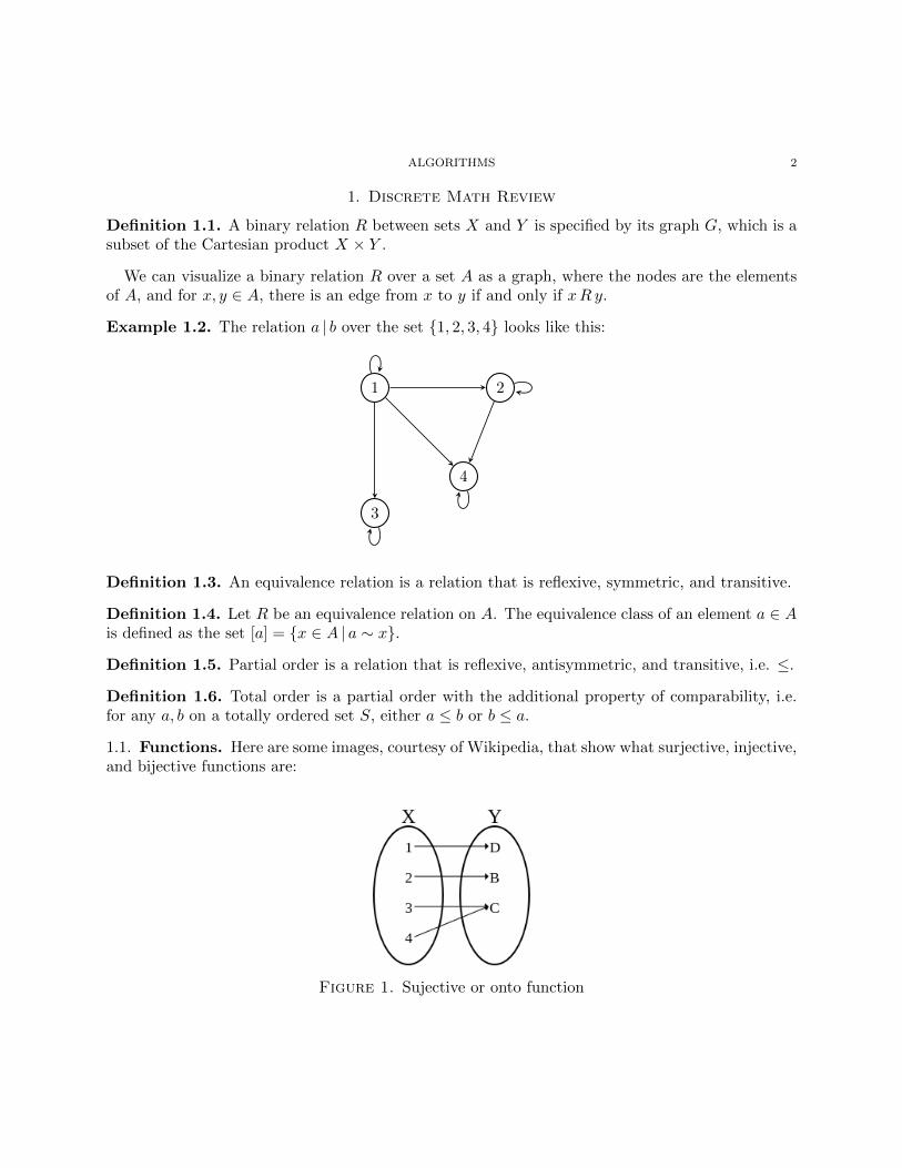
Example 1.2. The relation a | b over the set {1, 2, 3, 4} looks like this:

1 2

3

4

Definition 1.3. An equivalence relation is a relation that is reflexive, symmetric, and transitive.

Definition 1.4. Let R be an equivalence relation on A. The equivalence class of an element a 2 Ais defined as the set [a] = {x 2 A | a ⇠ x}.

Definition 1.5. Partial order is a relation that is reflexive, antisymmetric, and transitive, i.e. .

Definition 1.6. Total order is a partial order with the additional property of comparability, i.e.for any a, b on a totally ordered set S, either a b or b a.

1.1. Functions. Here are some images, courtesy of Wikipedia, that show what surjective, injective,and bijective functions are:

Figure 1. Sujective or onto function

ALGORITHMS 3

Figure 2. Injective or one-to-one function

Figure 3. Bijective function or a one-to-one correspondence

A set is countable if there is an injection from the set to the positive integers, otherwise the setis called uncountable.

Definition 1.7. A sequence is an ordered collection of objects, i.e. a function f : Z�0 ! X whereX is an arbitrary set. If f(n) = xn, for n 2 Z�0, we denote the sequence f with {xn}.1.2. Basic Graphs and Definitions.

Definition 1.8. Connectivity in graphs

(1) Connected undirected graph — each pair of vertices connected by path(2) Connected components — equivalence class of vertices under “is reachable from” relation(3) Strongly connected components of directed graph — equivalence class of vertices under “are

mutually reachable” relation(4) Strongly connected directed graph — every two vertices reachable from one another, exactly

one strongly connected component

Definition 1.9. A graph isomorphism between graphs G and H is a bijection between the vertexsets of G and H,

f : V (G)! V (H)

such that any two vertices u, v 2 G are adjacent in G if and only if f(u) and f(v) are adjacent inH.

ALGORITHMS 4

Definition 1.10. Special graphs

(1) Complete graph — an undirected graph with every pair of vertices adjacent(2) Bipartite graph — undirected graph in which the vertex set is partitioned into two sets V1

and V2 such that every edge are of the form (x, y) where x 2 V1 and y 2 V2

(3) Tree — connected, acyclic undirected graph(4) Forest — acyclic undirected graph (i.e. made up of many trees)(5) DAG — directed acyclic graph(6) Multigraph — like undirected graph, but can have multiple edges between vertices as well

as self-loops(7) Hypergraph — like undirected graph, but each hyperedge can connect arbitrary number of

vertices

Example 1.11. If G is an undirected graph on n nodes, where n is an even number, prove that ifevery node of G has degree of at least n/2, then G is connected. Prove this by contradiction.

Proof. Suppose every node of G has degree of at least n/2 and G is not connected. Let u and vbe from separate components of G. Let U and V be the set of neighbors of u and v respectively.Since the nodes in U and V are separate, |U \ V | = 0. Recall

|U \ V | = |U |+|V |�|U [ V |by the inclusion-exclusion principle. Notice that |U | = |V | = n/2 by our supposition, which implies

|U \ V | = n�|U [ V | .Since u and v are not included in U [ V , then |U [ V | n� 2. It follows that 2 is the lower boundfor |U \ V |, i.e. |U \ V | � 2. A contradiction. ⇤Proposition 1.12. Every connected graph G = (V,E) with |V | � 2 has two vertices x1 and x2 so

that G \ {x1} is connected and G \ {x2} is connected.

Proof. Base case: Let G be a connected graph with V = {x1, x2}. Then G \ {x1} and G \ {x2}are both trivially connected.

Inductive step: Suppose every connected graph G with |V | = n has two vertices x1 and x2 sothat G \ {x1} and G \ {x2} are connected. Let G0 be a graph as defined in the previous statementbut with one additional connected node v0.

v0 has either an edge connected to G \ {x1, x2} or is connected to either (or both) x1 or x2. If v0

is connected to G \ {x1, x2}, then v0 is still connected when x1 or x2 is removed. Without loss ofgenerality, consider the case when v0 has an edge with x1. Then we can change the vertex that weare removing to be v0 instead of x1, i.e. G \ {v0} will still be connected. Thus we have shown thatif G is connected with |V | � 2 that there are two vertices so that their indiviual removal results ina connected graph. ⇤Example 1.13. A connected, undirected graph is vertex biconnected if there is no vertex whoseremoval disconnects the graph. A connected, undirected graph is edge biconnected if there is noedge whose removal disconnects the graph.

(1) Prove a vertex biconnected graph is edge biconnected for graphs with more than one edge.(2) Give a counterexample that an edge biconnected graph is vertex biconnected.

ALGORITHMS 5

Proof. (1) Suppose a vertex biconnected graph is not edge biconnected for graphs with more thanone edge. Let G be such a graph and V its set of vertices and E is its set of edges. Then thereis an edge e = (a, b), where a, b 2 V such that the graph G with edges E \ {e} is not connected.Notice that G is now made of two connected components with one edge e connecting them. Notethat if we remove either a or b that the edge e is implicitly removed, and the graph would no longerbe connected. This contradicts our supposition that G was vertex biconnected. Thus a vertexbiconnected graph is edge biconnected for graphs with more than one edge. ⇤

(2)

v0

v1

v2

v3

v4

Remove node v0 in the above edge biconnected graph and we see it is not vertex biconnected.

Example 1.14. We have a connected graph G = (V,E) and a specific vertex v 2 V . Supposewe compute a depth-first search tree rooted at u and obtain a tree T that includes all nodes ofG. Suppose we then compute a breadth-first search tree rooted at u and obtain the same tree T .Prove that G = T . (In other words, if T is both a depth-first search tree and a breadth-first searchtree rooted at u, then G cannot contain any edges that do not belong to T .)

Proof. Suppose G is a connected graph and its depth-first search (DFS) tree T rooted at vertex uis the same as the breadth-first search (BFS) tree rooted at u, yet G 6= T . Then G has at leastone edge not included in T . Let E be the set of edges for G, E0 be the set of edges for T , andX = E \ E0 be this set of missing edges. Note that X 6= ?. Then the graph with E0 [ X willcontain at least one cycle. Let C be one such cycle. In DFS, the vertices of C will be in the samepath in T . However, this will not be the case in BFS, as the node that is started on will have abranch that contains one of the vertices of C. A contradiction. Thus G = T . ⇤

2. Stable Marriage

Theorem 2.1. The set of pairs returned by the Gale-Shapley algorithm is a stable matching.

Proof. Suppose not, that is suppose all matchings have unstable pairs. Let M be the set of menand W be the set of women, both with equal size. Since the matching contains unstable pairs,there exist two pairs of men and women (m,w) 2 M ⇥W and (m0, w0) 2 M ⇥W such that mprefers w0 and m0 prefers w, by the definition of unstable. Note, by our algorithm, that m musthave proposed to w last. Since m prefers w0, m must have proposed to w0 earlier; however, sincem is no longer proposed to w0, this implies that w0 prefers another man more than m. Choosethis preferred man m00 2M . Since w0 is engaged with m0, either m00 = m0 or w0 prefers m0 to m00.Notice that this contradicts our supposition that w0 prefers m. Thus the set of pairs returned bythe Gale-Shapley algorithm is a stable matching. ⇤Example 2.2. Disprove the following: In every instance of the “Stable Marriage” problem, thereis a stable matching containing a pair (m,w) such that m is ranked first on the preference list ofw and w is ranked first on the preference list of m.

ALGORITHMS 6

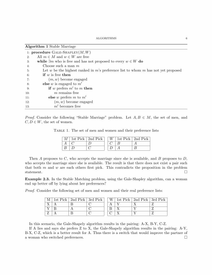
Algorithm 1 Stable Marriage

1: procedure Gale-Shapley(M,W )2: All m 2M and w 2W are free3: while 9m who is free and has not proposed to every w 2W do4: Choose such a man m5: Let w be the highest ranked in m’s preference list to whom m has not yet proposed6: if w is free then7: (m,w) become engaged8: else w is engaged to m0

9: if w prefers m0 to m then10: m remains free11: else w prefers m to m0

12: (m,w) become engaged13: m0 becomes free

Proof. Consider the following “Stable Marriage” problem. Let A,B 2 M , the set of men, andC,D 2W , the set of women.

Table 1. The set of men and women and their preference lists

M 1st Pick 2nd Pick W 1st Pick 2nd PickA C D C B AB D C D A B

Then A proposes to C, who accepts the marriage since she is available, and B proposes to D,who accepts the marriage since she is available. The result is that there does not exist a pair suchthat both m and w are each others first pick. This contradicts the proposition in the problemstatement. ⇤Example 2.3. In the Stable Matching problem, using the Gale-Shapley algorithm, can a womanend up better o↵ by lying about her preferences?

Proof. Consider the following set of men and women and their real preference lists:

M 1st Pick 2nd Pick 3rd Pick W 1st Pick 2nd Pick 3rd PickX A B C A Y X ZY B A C B X Y ZZ A B C C X Y Z

In this scenario, the Gale-Shapely algorithm results in the pairing: A-X, B-Y, C-Z.If A lies and says she prefers Z to X, the Gale-Shapely algorithm results in the pairing: A-Y,

B-X, C-Z, which is a better result for A. Thus there is a switch that would improve the partner ofa woman who switched preferences. ⇤

ALGORITHMS 7

3. Asymptotic Growth of Functions

• f(n) = o(g(n)) if and only if lim supn!1

f(n)g(n) = 0.

• f(n) = O(g(n)) if and only if lim supn!1

f(n)g(n) <1.

• f(n) = ⇥(g(n)) if and only if 0 < lim supn!1

f(n)g(n) <1.

• f(n) = ⌦(g(n)) if and only if lim supn!1

f(n)g(n) > 0.

• f(n) = !(g(n)) if and only if lim supn!1

f(n)g(n) =1.

Here are some properties of the above:

• Transpose symmetry — f(n) = O(g(n)) () g(n) = ⌦(f(n))• If f = O(h) and g = O(h), then f + g = O(h)• If g = O(f), then f + g = ⇥(f)

Recall that you change bases of logarithms with: logb a = logc alogc b

.

Remark 3.1. Note that an algorithm that requires an operation such as�nk

�, then that algorithm

is polynomial time as O(nk).

Theorem 3.2. Any comparison sort algorithm is ⌦(n log n).

Proof. Assume the input to the algorithms are distinct numbers 1, . . . , n. Then there are n! permu-tations of these numbers. Let h be the height of the decision tree that corresponds to the algorithm.Notice that

n! the total number of leaves on the decision tree 2h =)h � log n! = log n+ log n� 1 + · · ·+ log 2

=nX

i=2

log i

=

n/2�1X

i=2

log i+nX

n/2

log i

�nX

n/2

logn

2

=n

2log

n

2= ⌦(n log n).

⇤Example 3.3. You are given 9 identical looking balls and told that one of them is slightly heavierthan the others. Your task is to identify the defective ball. All you have is a balanced scale thatcan tell you which of the two sides of the scale is heavier (any number of balls can be placed oneach side of the scale).

ALGORITHMS 8

(1) Show how to identify the heavier ball in just 2 weighings.(2) Give a decision tree lower bound showing that it is not possible to determine the defective

ball in fewer than 2 weighings.

(1) Let B = {b1, . . . , b9} be the set of balls. First we weigh 13 of the balls. Without loss of

generality, we can say we first weigh balls B1 = {b1, b2, b3} and B2 = {b4, b5, b6}. Let B3 be theremaining set of balls, i.e. B3 = {b6, b7, b8}. Define W (·) to be the mapping that weighs a ball orgroup of balls.

If W (B1) = W (B2), then we split B3 into thirds and weigh two balls, WLOG say b7 and b8. Ifb7 = b8, then b9 is the heaviest ball.

If W (B1) 6= W (B2), then choose the heavier group and do the algorithm done to set B3.

(2) Let B1, B2, B3, and W (·) be defined as above and let H(·) represent the heaviest ball.

W (B1)?= W (B2)

W (b1)?= W (b2)

H(b1)W (b1) > W (b2)

H(b2)W (b1) < W (b2)

H(b3)W (b1) = W (b2)

W(B

1 ) >W(B

2 )

W (b4)?= W (b5)

H(b4)W (b4) > W (b5)

H(b5)W (b4) < W (b5)

H(b6)W (b4) = W (b5)

W (B1) < W (B2)

W (b7)?= W (b8)

H(b7)W (b7) > W (b8)

H(b8)W (b7) < W (b8)

H(b9)W (b7) = W (b8)

W(B1)

=W(B2)

It is clear from the decision tree that there are no ways to reduce the amount of weighings from2.

4. Data Structures

Definition 4.1. A priority queue is like a queue or stack, except each element also has a priorityassociated with it; an element with higher priority is served before an element with low priority.

ALGORITHMS 9

Definition 4.2. A heap is a specialized tree-based data structure that satisfies the heap property:If A is a parent node of B then the key (the value) of node A is ordered with respect to the key ofnode B with the same ordering applied across the heap.

A heap is a convenient data structure on which to implement a priority queue.

Example 4.3. Here is an example of a heap, all parents are smaller than their children:

1 5 2 10 9 7 11

This is implemented such that if the parent is stored at index i, then the two children at most arestored at 2i and 2i+ 1. Here is the graph associated with the heap above.

1

5

10 9

2

7 11

To insert a new element on a heap, we implement an algorithm called heapify-up. The elementis added to the bottom level of the heap (at the left most freely available spot). The element iscompared to its parent; if they are in the correct order, then we are done. However, if not, then weswap the element with its parent and start again at the last step until we are done.

To remove an element on the heap, we implement an algorithm called heapify-down. First wereplace the root of the heap with the last element on the last level. Then we compare the new rootwith its children; if they are in the correct order, then we are done. However, if not, then we swapthe element with one of its children and return to the previous step. (The swap depends on theordering of the heap)

Example 4.4. Give an e�cient algorithm to find all keys in a min-heap that are smaller than aprovided value. The provided value does not have to be a key in the min-heap. Evaluate the timecomplexity of your algorithm.

Recall a min-heap is a complete binary tree in which the data contained in each node is less than(or equal to) the data in that node’s children.

Algorithm 2 Find all smaller values in a min-heap

1: procedure Find smaller(root, value)2: if root > value then3: return4: Find smaller(root’s left node, value)5: Find smaller(root’s right node, value)6: return root

ALGORITHMS 10

Let n be the number of nodes in the min-heap. This algorithm’s time complexity is O(n), sinceat worst case the value will be greater than every node in the min-heap.

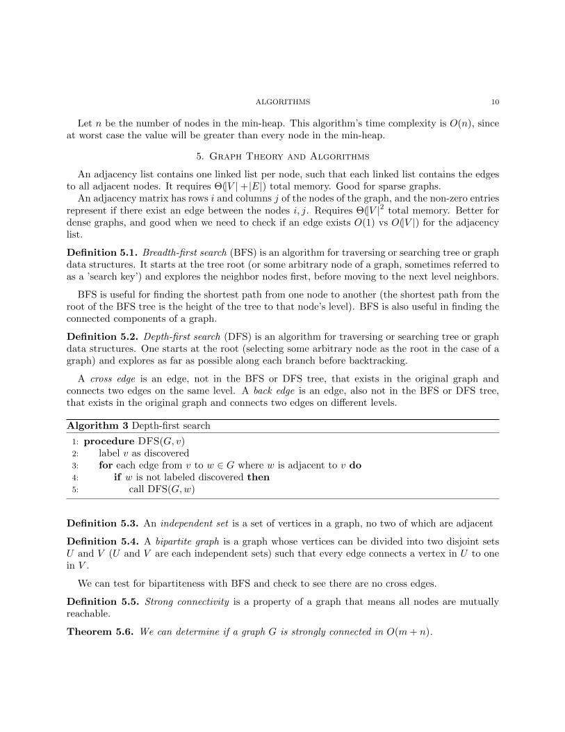
5. Graph Theory and Algorithms

An adjacency list contains one linked list per node, such that each linked list contains the edgesto all adjacent nodes. It requires ⇥(|V |+|E|) total memory. Good for sparse graphs.

An adjacency matrix has rows i and columns j of the nodes of the graph, and the non-zero entriesrepresent if there exist an edge between the nodes i, j. Requires ⇥(|V |2 total memory. Better fordense graphs, and good when we need to check if an edge exists O(1) vs O(|V |) for the adjacencylist.

Definition 5.1. Breadth-first search (BFS) is an algorithm for traversing or searching tree or graphdata structures. It starts at the tree root (or some arbitrary node of a graph, sometimes referred toas a ’search key’) and explores the neighbor nodes first, before moving to the next level neighbors.

BFS is useful for finding the shortest path from one node to another (the shortest path from theroot of the BFS tree is the height of the tree to that node’s level). BFS is also useful in finding theconnected components of a graph.

Definition 5.2. Depth-first search (DFS) is an algorithm for traversing or searching tree or graphdata structures. One starts at the root (selecting some arbitrary node as the root in the case of agraph) and explores as far as possible along each branch before backtracking.

A cross edge is an edge, not in the BFS or DFS tree, that exists in the original graph andconnects two edges on the same level. A back edge is an edge, also not in the BFS or DFS tree,that exists in the original graph and connects two edges on di↵erent levels.

Algorithm 3 Depth-first search

1: procedure DFS(G, v)2: label v as discovered3: for each edge from v to w 2 G where w is adjacent to v do4: if w is not labeled discovered then5: call DFS(G,w)

Definition 5.3. An independent set is a set of vertices in a graph, no two of which are adjacent

Definition 5.4. A bipartite graph is a graph whose vertices can be divided into two disjoint setsU and V (U and V are each independent sets) such that every edge connects a vertex in U to onein V .

We can test for bipartiteness with BFS and check to see there are no cross edges.

Definition 5.5. Strong connectivity is a property of a graph that means all nodes are mutuallyreachable.

Theorem 5.6. We can determine if a graph G is strongly connected in O(m+ n).

ALGORITHMS 11

Algorithm 4 Test for Strongly Connected Graph

1: procedure Strongly connected test(G, v)2: Run BFS from v3: Run BFS from v but reverse the directions of the edges of G4: return true if and only if all nodes reached in both BFS trees

Definition 5.7. A topological ordering of a directed graph is a linear ordering of its vertices suchthat for every directed edge (u, v) from vertex u to vertex v, u comes before v in the ordering.

Remark 5.8. Any DAG has at least one topological ordering, and there exist algorithms for con-structing a topological ordering of any DAG in O(n).

6. Greedy algorithms

Definition 6.1. A problem is said to have optimal substructure if an optimal solution can beconstructed e�ciently from optimal solutions of its subproblems.

Definition 6.2. A problem has the greedy-choice property if a global optimum can be arrived atby selecting a local optimum.

If a problem has both an optimal substructure and the greedy-choice property, then the problemcan be solved with a greedy algorithm.

Example 6.3. To find a solution to the problem of interval scheduling, a greedy algorithm willpick the job with the earliest finish time.

Algorithm 5 Interval scheduling algorithm

1: procedure Interval scheduler(Jobs)2: Sort jobs by finish time3: Selected Jobs ?4: for each job j do5: if j is compatible with Selected Jobs then6: Selected Jobs [ {j}

To show that a greedy algorithm is optimal, we must show that the greedy algorithm stays aheador is equal to any solution that can be constructed.

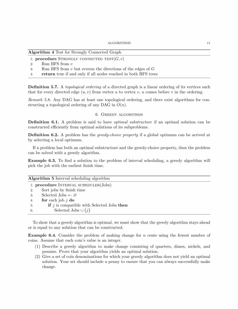
Example 6.4. Consider the problem of making change for n cents using the fewest number ofcoins. Assume that each coin’s value is an integer.

(1) Describe a greedy algorithm to make change consisting of quarters, dimes, nickels, andpennies. Prove that your algorithm yields an optimal solution.

(2) Give a set of coin denominations for which your greedy algorithm does not yield an optimalsolution. Your set should include a penny to ensure that you can always successfully makechange.

ALGORITHMS 12

(1)

Algorithm 6 Make change with American coins

1: procedure Make change(n)2: Initialize C as an empty array to hold the change3: while n > 0 do4: if n � 25 then5: n n� 256: Add a quarter to C7: else if n � 10 then8: n n� 109: Add a dime to C

10: else if n � 5 then11: n n� 512: Add a nickel to C13: else14: n n� 115: Add a penny to C

Proposition 6.5. The Make change algorithm yields an optimal solution.

Proof. To show that Make change yields an optimal solution, we need to show that the problemhas an optimal substructure and that the greedy choice property holds.

Let C = {c1, c2, . . . , ck} be the optimal solution for the amount n. The optimal substructure ofthe problem can be seen by noticing that we can remove a coin from C, without loss of generalitysay C 0 = C \ {ck}, and noticing that C 0 is the optimal solution for the amount n0 = n� value(ck).

If C 0 were not the optimal solution for n0, then there would exist an optimal solution, say C 00 forn0. However, if C 00 is more optimal than C 0, we can add ck back to C 00 for a more optimal solutionto the amount n. Which contradicts our supposition that C is the optimal solution to the amountn.

Now we will show that the greedy choice property applies to the problem. Suppose the greedychoice is not in the optimal solution S. Since the greedy choice has not been followed, this meansthat lower value coins G ⇢ S were used to make change for some higher value coin c. However,we can replace G with our high value coin c to yield a more optimal solution. Thus the greedychoice property holds. Since we have shown the problem has both an optimal substructure and thegreedy choice property, it follows that the greedy algorithm Make change produces an optimalsolution. ⇤

(2) Let the set of coin denominations be {1, 4, 5, 7} and get change for 9 cents. The greedyalgorithm will pick 7 and then 1 twice for a total of 3 coins. However, the optimal solution ispicking the 4 and 5 cent coins for a total of 2 coins.

Example 6.6. Let X be a set of n intervals on the real line. A subset of intervals Y ✓ X is calleda tiling path if the intervals in Y cover the intervals in X, that is, any real value that is contained

ALGORITHMS 13

in some interval in X is also contained in some interval in Y . The size of a tiling cover is just thenumber of intervals.

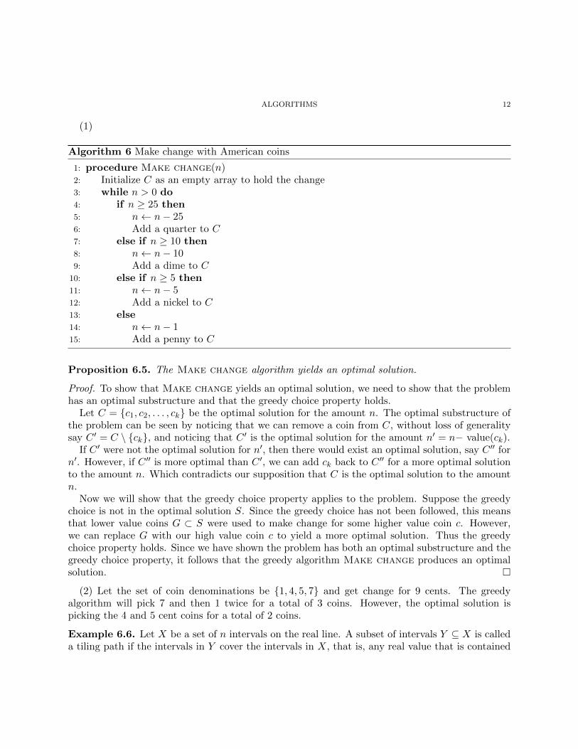
Describe an algorithm to compute the smallest tiling path of X. Argue that your algorithm iscorrect

Algorithm 7 Find the smallest path that tiles an interval

1: procedure Find smallest tiling path(X)2: T end of interval X3: t start of interval X4: Initialize Y = ?, the set that holds the tiling intervals5: while t < T do6: y farthest right stretching interval starting from or before t in X7: Y [ {y}8: t end of y

Proposition 6.7. The Find smallest tiling path algorithm solves the problem correctly.

Proof. We must first show that the problem that is to be solved has an optimal substructure, thenwe will show that the greedy choice property holds.

Notice that Find smallest tiling path breaks up the tiling problem into smaller problems bychanging the interval of search for smaller regions when we update t.

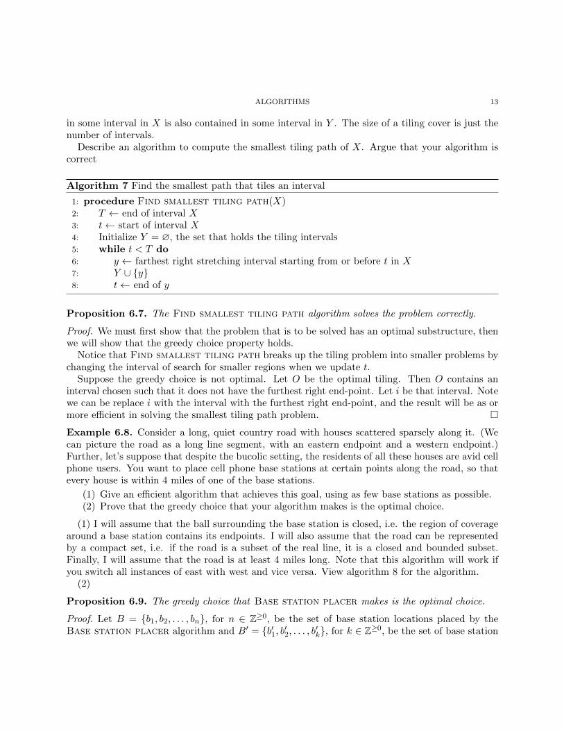
Suppose the greedy choice is not optimal. Let O be the optimal tiling. Then O contains aninterval chosen such that it does not have the furthest right end-point. Let i be that interval. Notewe can be replace i with the interval with the furthest right end-point, and the result will be as ormore e�cient in solving the smallest tiling path problem. ⇤Example 6.8. Consider a long, quiet country road with houses scattered sparsely along it. (Wecan picture the road as a long line segment, with an eastern endpoint and a western endpoint.)Further, let’s suppose that despite the bucolic setting, the residents of all these houses are avid cellphone users. You want to place cell phone base stations at certain points along the road, so thatevery house is within 4 miles of one of the base stations.

(1) Give an e�cient algorithm that achieves this goal, using as few base stations as possible.(2) Prove that the greedy choice that your algorithm makes is the optimal choice.

(1) I will assume that the ball surrounding the base station is closed, i.e. the region of coveragearound a base station contains its endpoints. I will also assume that the road can be representedby a compact set, i.e. if the road is a subset of the real line, it is a closed and bounded subset.Finally, I will assume that the road is at least 4 miles long. Note that this algorithm will work ifyou switch all instances of east with west and vice versa. View algorithm 8 for the algorithm.

(2)

Proposition 6.9. The greedy choice that Base station placer makes is the optimal choice.

Proof. Let B = {b1, b2, . . . , bn}, for n 2 Z�0, be the set of base station locations placed by theBase station placer algorithm and B0 = {b01, b02, . . . , b0k}, for k 2 Z�0, be the set of base station

ALGORITHMS 14

Algorithm 8 Place base stations to create an optimal solution

1: procedure Base station placer(Road)2: Start at the western most point of the road3: while not at the eastern end of the road do4: Travel east until we are exactly 4 miles east of an uncovered house5: Place a base station at our current location6: Ignoring all houses covered by this base station, repeat this process

location for the optimal solution. Note that both B and B0’s elements are indexed from west toeast. Without loss of generality, assume that the western-most point is 0 and the eastern-mostpoint is some positive real number N . It follows that the locations of the base stations bi are realnumbers between 0 and N . Now we will show that the solution provided by B is the same or betterto the solution provided by B0.

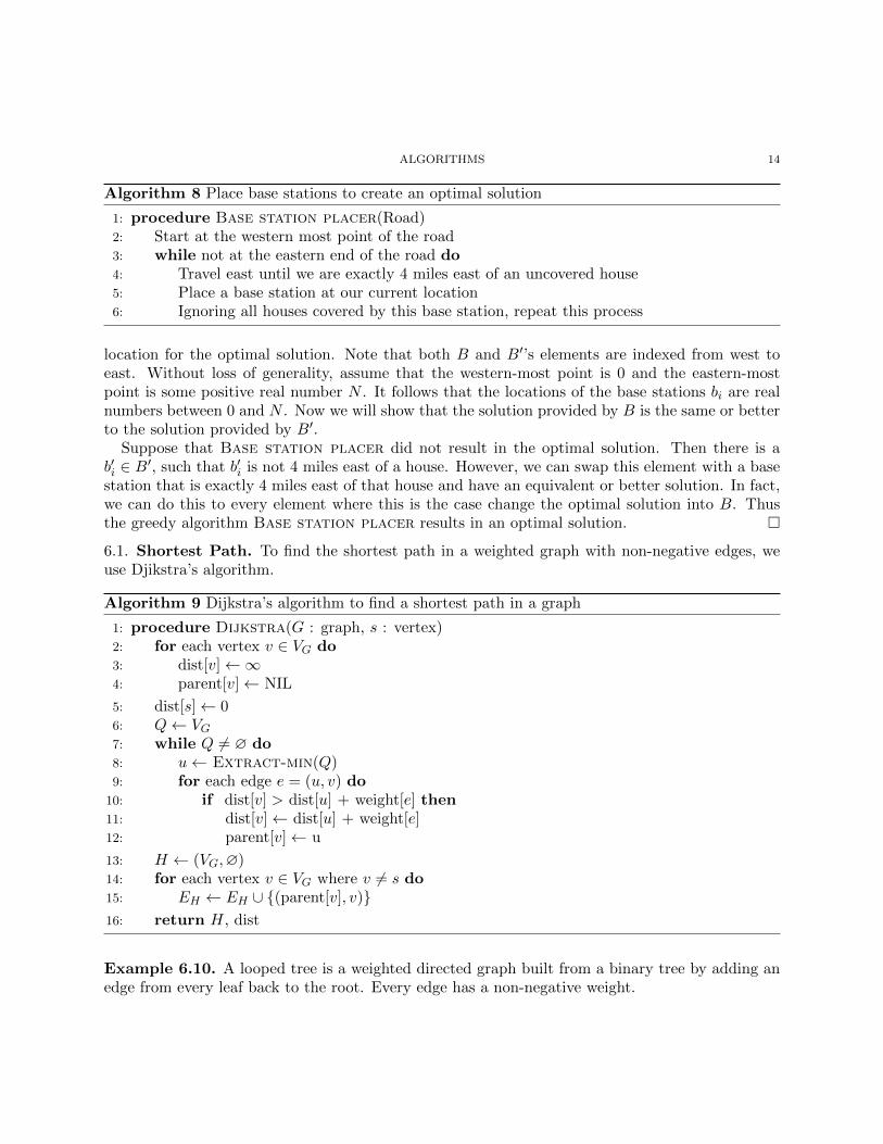
Suppose that Base station placer did not result in the optimal solution. Then there is ab0i 2 B0, such that b0i is not 4 miles east of a house. However, we can swap this element with a basestation that is exactly 4 miles east of that house and have an equivalent or better solution. In fact,we can do this to every element where this is the case change the optimal solution into B. Thusthe greedy algorithm Base station placer results in an optimal solution. ⇤6.1. Shortest Path. To find the shortest path in a weighted graph with non-negative edges, weuse Djikstra’s algorithm.

Algorithm 9 Dijkstra’s algorithm to find a shortest path in a graph

1: procedure Dijkstra(G : graph, s : vertex)2: for each vertex v 2 VG do3: dist[v] 14: parent[v] NIL

5: dist[s] 06: Q VG

7: while Q 6= ? do8: u Extract-min(Q)9: for each edge e = (u, v) do

10: if dist[v] > dist[u] + weight[e] then11: dist[v] dist[u] + weight[e]12: parent[v] u

13: H (VG,?)14: for each vertex v 2 VG where v 6= s do15: EH EH [ {(parent[v], v)}16: return H, dist

Example 6.10. A looped tree is a weighted directed graph built from a binary tree by adding anedge from every leaf back to the root. Every edge has a non-negative weight.

ALGORITHMS 15

(1) How much time would Dijkstra’s algorithm require to compute the shortest path from u tov in a looped tree with n nodes? (Do NOT assume that either u or v is the root of the treethough one could be.)

(2) Describe and analyze a faster algorithm to find the shortest path from u to v in a loopedtree.

(1) Dijkstra’s algorithm’s complexity is O(|E| log n). In this case |E| = O(n), so it follows thatthe overall complexity for this will be O(n log n).

(2)

Algorithm 10 Find the shortest path in a looped tree

1: procedure Looped tree shortest path(T , u, v)2: D DFS(T ) starting at root3: if u is an ancestor of v then4: Choose path directly down D from u to v5: else6: S subtree of u with the root as the children of the leaves (not connected to rest of T )7: Path Topological sort shortest path(S)8: Take Path to get from u to root, then follow the path in D from root to v.

DFS is known to be O(n) and Topological sort shortest path is O(n + |E|). Since|E| = O(n), Looped tree shortest path is O(n).

6.2. Minimum Spanning Tree. There are two main algorithms for finding the minimum span-ning tree of a graph: (1) Kruskal’s algorithm and (2) Prim’s algorithm. Here are (oversimplified)overviews of the two algorithms.

Kruskal’s algorithm. For a graph G, start with |V | trees (one for each vertex). Consider edges Ein increasing order of weights, and add an edge if it connects two trees.

Prim’s algorithm. Start with spanning tree containing arbitrary vertex v and no edges. Growspanning tree by repeatedly adding minimal weight edge connecting vertex v in current spanningtree with a vertex not in the tree.

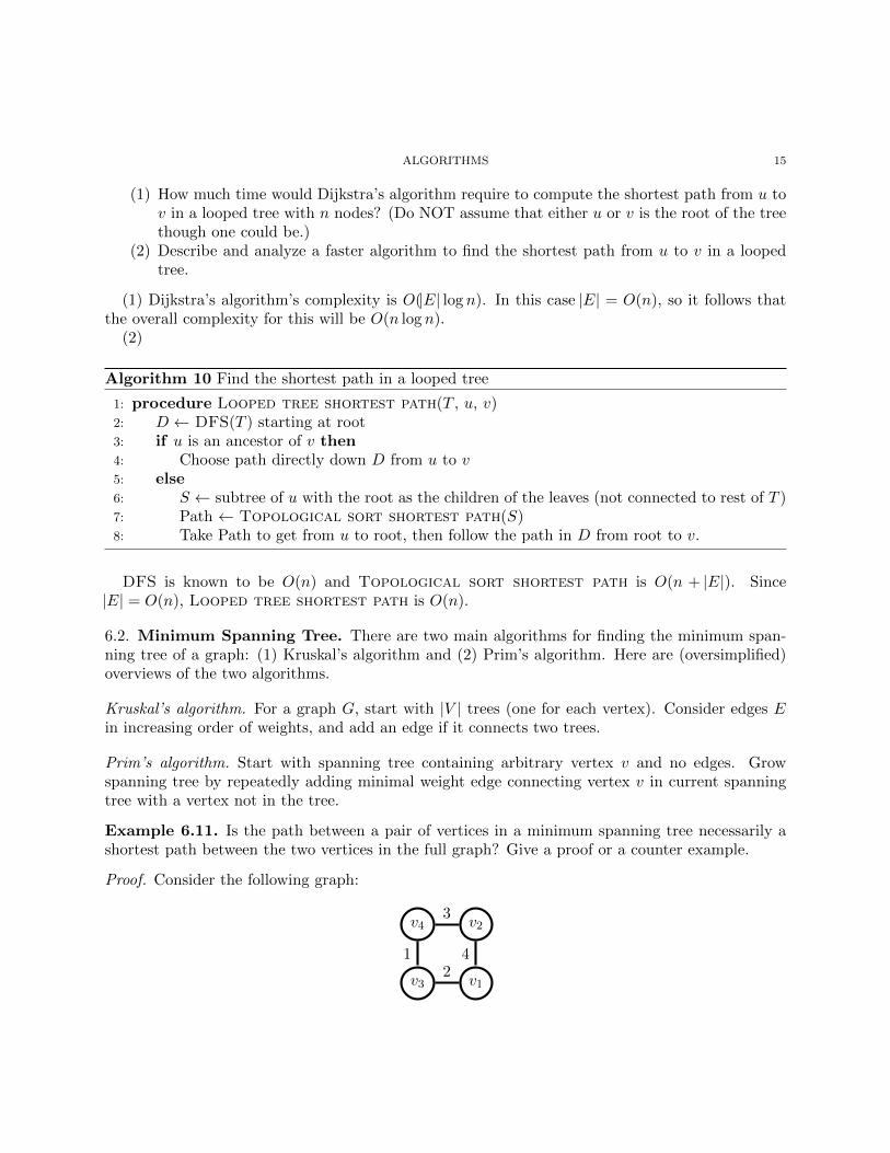
Example 6.11. Is the path between a pair of vertices in a minimum spanning tree necessarily ashortest path between the two vertices in the full graph? Give a proof or a counter example.

Proof. Consider the following graph:

v1

v2

v3

v4

12

3

4

ALGORITHMS 16

Note that the minimum spanning tree contains the edges weighted by 1, 2, 3. However, the edgebetween v1 and v2, weighted with 4, is the shortest path between the two nodes. Thus the pathbetween a pair of vertices in a minimum spanning tree is not necessarily a shortest path betweenthe two vertices in the full graph. ⇤Example 6.12. Let us say that a graph G = (V,E) is a near-tree if it is connected and has atmost n+8 edges, where n = |V |. Give an algorithm with running time O(n) that takes a near-treeG with costs on its edges and returns a minimum spanning tree of G. You may assume that all ofthe edge costs are distinct.

Algorithm 11 Algorithm to find a minimum spanning tree in a near-tree

1: procedure Near-tree minimum spanning tree(G)2: B BFS(G)3: for each edge e of G not found in B do4: Insert e into B5: Find the greatest weight edge in the cycle created by the insertion and remove it

Since there are at most 9 edges to check, the above algorithm runs in O(n), due to running BFS.

6.3. Fractional Knapsack. Suppose you are a thief, and you have a knapsack with a weightcapacity. You want to maximize the value you can steal. If you can fill a knapsack with fractionsof items instead of whole items, we can solve the problem with a greedy solution. Just fill yourknapsack with the highest value per weight first, then fill with the next highest value per weight,and so on, until the knapsack is full.

6.4. Hu↵man Codes. Hu↵man codes are a variable length data compression scheme. It relies onfinding the probability of each character appearing in the file to be compressed, and using less bitsfor characters that appear with higher probability, and more for characters that appear with lessprobability.

Algorithm 12 Hu↵man encoding algorithm

1: procedure Huffman(C : characters to encode)2: n |C|3: Q C . initialize heap with elements of C, probability as key4: for i 1 to n� 1 do5: allocate new node z6: left[z] x Extract-Min(Q)7: right[z] y Extract-Min(Q)8: f [z] f [x] + f [y]9: Insert(Q, z)

10: return Extract-Min(Q)

Note Huffman is O(|V | log |V |).

ALGORITHMS 17

Example 6.13. Consider the binary tree that is constructed in the Hu↵man coding procedure.Prove that a binary tree that is not full cannot correspond to an optimal prefix code.

Proof. Suppose that there is a binary tree that is not full that does correspond to an optimal prefixcode. Let that tree be designated by T , with the node v which only has one child c. However, wecan replace v with c and have a more optimal code, since less bits will be needed to represent thevalue of c. A contradiction. ⇤

7. Divide and Conquer

The divide-and-conquer strategy solves a problem by:

(1) Breaking it into subproblems that are themselves smaller instances of the same type ofproblem

(2) Recursively solving these subproblems(3) Appropriately combining their answers

Divide-and-conquer, generally, can only reduce time complexity from a higher polynomial to alower polynomial.

7.1. Exponentiation. We can speed up the polynomial time (in this case O(n)) operation ofnormal exponentiation with a divide and conquer algorithm.

Algorithm 13 Implementation of an exponentiation function with divide and conquer

1: function Fast Power(a, n)2: if n = 1 then3: return a4: x FastPower(a, bn/2c)5: if n is even then6: return x · x7: else8: return x · x · a

7.2. Merge-sort. Divide the unsorted list into n sublists, each containing 1 element (a list of 1element is considered sorted). Repeatedly merge sublists to produce new sorted sublists until thereis only 1 sublist remaining. This will be the sorted list.

Example 7.1. Give an e�cient algorithm to find the kth largest element in the merge of two sortedsequences S1 and S2. The best algorithm runs in O(log(max(m,n))), where |S1| = n and |S2| = m.

We will assume that k |S1|+ |S2|, either S1 or S2 is non-empty, and both S1 and S2 are sortedfrom largest to smallest. When each sequence is sorted in this way, the kth largest element is inthe kth index (or potentially in the k � 1th spot, if indexed as most programming languages).

ALGORITHMS 18

Algorithm 14 Find the kth largest element in two sorted arrays

1: function Find kth largest(S1, S2, k)2: if S1 = ? and S2 6= ? then3: return S2[k]4: else if S2 = ? and S1 6= ? then5: return S1[k]

6: m1 middle index of S1

7: m2 middle index of S2

8: if m1 +m2 < k then9: if S1[m1] S2[m2] then

10: return Find kth largest(S1[> m1], S2, k �m1 � 1)11: else12: return Find kth largest(S1, S2[> m2], k �m2 � 1)

13: else14: if S1[m1] S2[m2] then15: return Find kth largest(S1, S2[< m2], k)16: else17: return Find kth largest(S1[< m1], S2, k)

7.3. Algorithm analysis.

Master method overview. The master theorem concerns recurrence relations of the form:

T (n) = a T

✓n

b

◆+ f(n) where a � 1, b > 1

• n is the size of the problem.• a is the number of subproblems in the recursion.• n/b is the size of each subproblem. (Here it is assumed that all subproblems are essentiallythe same size.)

• f(n) is the cost of the work done outside the recursive calls, which includes the cost ofdividing the problem and the cost of merging the solutions to the subproblems.

There are three cases:

(1) If f(n) 2 O (nc) where c < logb a, then T (n) 2 ⇥⇣nlogb a

⌘.

(2) If for some constant k � 0, that f(n) 2 ⇥⇣nc logk n

⌘where c = logb a, then T (n) 2

⇥⇣nc logk+1 n

⌘.

(3) If f(n) 2 ⌦ (nc) where c > logb a and if af�nb

� kf(n) for some constant k < 1, then

T (n) 2 ⇥�f(n)

�.

Example 7.2. Use the master method to give asymptotic bounds the following recurrences:

(1) T (n) = 5T (n/2) + n

ALGORITHMS 19

(2) T (n) = 5T (n/2) + n2

(3) T (n) = 5T (n/2) + n3

(1) Here f(n) = n, a = 5, and b = 2. Since 1 < log2 5, we are in case 1. Thus T (n) 2 ⇥⇣nlog2 5

⌘.

(2) Here f(n) = n2, a = 5, and b = 2. Since 2 < log2 5, we are in case 1. Thus T (n) 2 ⇥⇣nlog2 5

⌘.

(3) Here f(n) = n3, a = 5, and b = 2. Since 3 > log2 5 and 58n

3 58n

3, we are in case 3. ThusT (n) 2 ⇥

�n3

�.

7.4. Closest Pairs. Given n points in the Euclidean plane, find pair with smallest distance be-tween them. Note that the brute force solution would require us to check all points with ⇥(n2)comparisons. See algorithm 15.

Algorithm 15 Find closest pairs using divide and conquer

1: procedure Closest pair(P : set of all points)2: Compute a vertical line in the plane L such that half points on each side of L3: �1 Closest pair(P1...L)4: �2 Closest pair(PL+1...n)5: � min(�1, �2)6: Delete all points further than � from L7: sort remaining points by y-coordinate8: Scan points in y order and compare distance between each point and next 11 neighbors

9: If any of these distances are less than �, update �10: return �

7.5. More Examples.

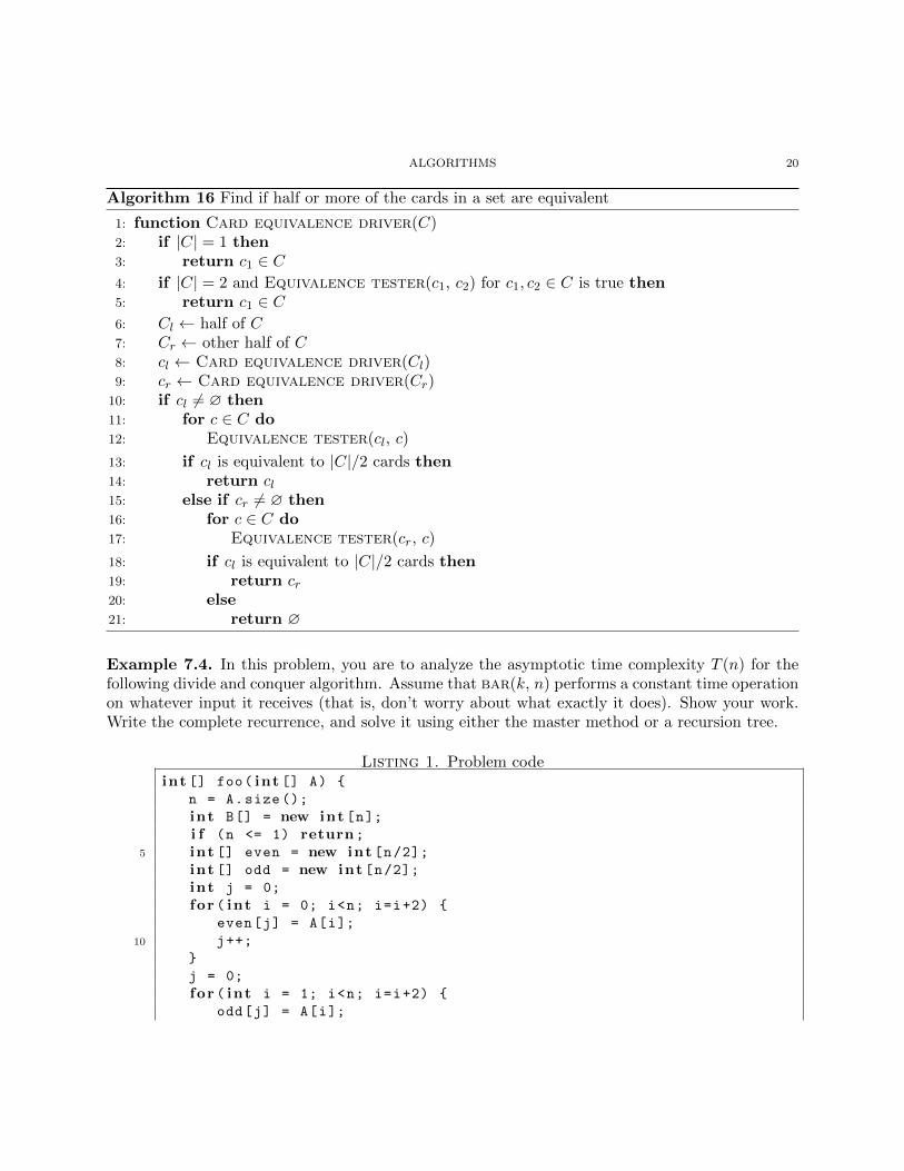
Example 7.3. Among the collection of n cards, is there a set of more than n/2 of them that areall equivalent to one another? Assume that the only feasible operations you can do with the cardsare to pick two of them and plug them in to the equivalence tester. Show how to decide the answerto their question with only O(n log n) invocations of the equivalence tester.

Let C be the set of cards.

ALGORITHMS 20

Algorithm 16 Find if half or more of the cards in a set are equivalent

1: function Card equivalence driver(C)2: if |C| = 1 then3: return c1 2 C

4: if |C| = 2 and Equivalence tester(c1, c2) for c1, c2 2 C is true then5: return c1 2 C

6: Cl half of C7: Cr other half of C8: cl Card equivalence driver(Cl)9: cr Card equivalence driver(Cr)

10: if cl 6= ? then11: for c 2 C do12: Equivalence tester(cl, c)

13: if cl is equivalent to |C|/2 cards then14: return cl15: else if cr 6= ? then16: for c 2 C do17: Equivalence tester(cr, c)

18: if cl is equivalent to |C|/2 cards then19: return cr20: else21: return ?

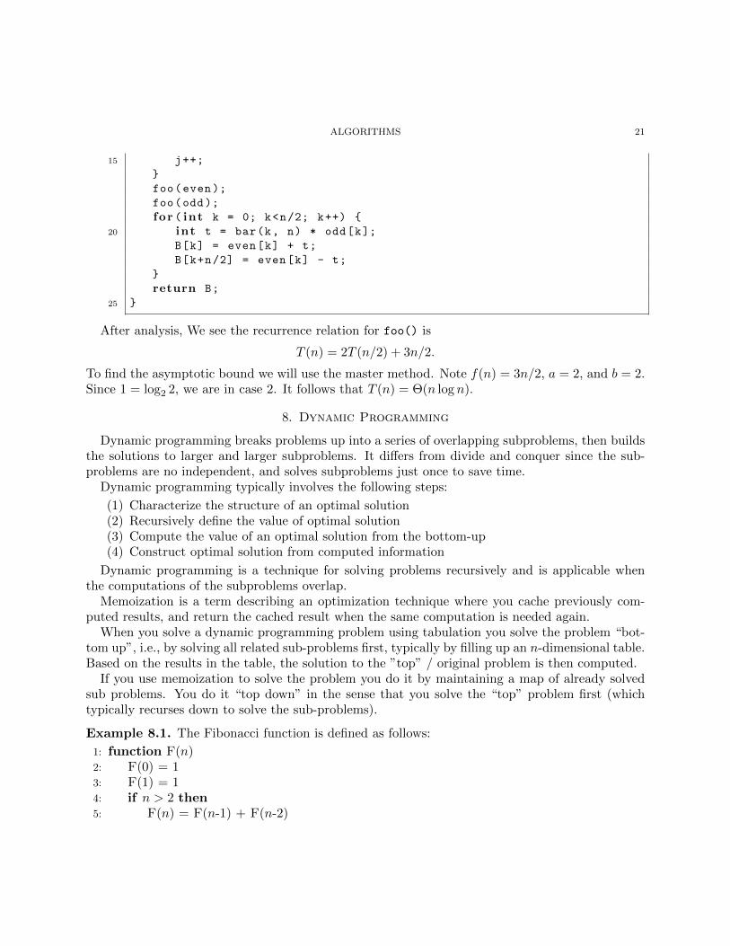
Example 7.4. In this problem, you are to analyze the asymptotic time complexity T (n) for thefollowing divide and conquer algorithm. Assume that bar(k, n) performs a constant time operationon whatever input it receives (that is, don’t worry about what exactly it does). Show your work.Write the complete recurrence, and solve it using either the master method or a recursion tree.

Listing 1. Problem codeint [] foo( int [] A) {

n = A.size ();

int B[] = new int [n];i f (n <= 1) return;

5 int [] even = new int [n/2];int [] odd = new int [n/2];int j = 0;

for ( int i = 0; i<n; i=i+2) {

even[j] = A[i];

10 j++;

}

j = 0;

for ( int i = 1; i<n; i=i+2) {

odd[j] = A[i];

ALGORITHMS 21

15 j++;

}

foo(even);

foo(odd);

for ( int k = 0; k<n/2; k++) {

20 int t = bar(k, n) * odd[k];

B[k] = even[k] + t;

B[k+n/2] = even[k] - t;

}

return B;

25 }

After analysis, We see the recurrence relation for foo() is

T (n) = 2T (n/2) + 3n/2.

To find the asymptotic bound we will use the master method. Note f(n) = 3n/2, a = 2, and b = 2.Since 1 = log2 2, we are in case 2. It follows that T (n) = ⇥(n log n).

8. Dynamic Programming

Dynamic programming breaks problems up into a series of overlapping subproblems, then buildsthe solutions to larger and larger subproblems. It di↵ers from divide and conquer since the sub-problems are no independent, and solves subproblems just once to save time.

Dynamic programming typically involves the following steps:

(1) Characterize the structure of an optimal solution(2) Recursively define the value of optimal solution(3) Compute the value of an optimal solution from the bottom-up(4) Construct optimal solution from computed information

Dynamic programming is a technique for solving problems recursively and is applicable whenthe computations of the subproblems overlap.

Memoization is a term describing an optimization technique where you cache previously com-puted results, and return the cached result when the same computation is needed again.

When you solve a dynamic programming problem using tabulation you solve the problem “bot-tom up”, i.e., by solving all related sub-problems first, typically by filling up an n-dimensional table.Based on the results in the table, the solution to the ”top” / original problem is then computed.

If you use memoization to solve the problem you do it by maintaining a map of already solvedsub problems. You do it “top down” in the sense that you solve the “top” problem first (whichtypically recurses down to solve the sub-problems).

Example 8.1. The Fibonacci function is defined as follows:

1: function F(n)2: F(0) = 13: F(1) = 14: if n > 2 then5: F(n) = F(n-1) + F(n-2)

ALGORITHMS 22

(1) Assume you implement a recursive procedure for computing the Fibonacci sequence baseddirectly on the function defined above. Then the running time of this algorithm can beexpressed as:

T (n) = T (n� 1) + T (n� 2) + 1

Determine the asyptotic bound that best satisfies the above recurrance relation.(2) What specifically is bad about your algorithm? (i.e., what observation can you make to

radically improve its running time?)(3) Give a memoized recursive algorithm for computing F(n) e�ciently. Write the recurrence

for your algorithm and give its asymptotic upper bound.(4) Give a traditional bottom-up dynamic programming algorithm for computing F(n) e�-

ciently. Write the recurrence for your algorithm and give its asymptotic upper bound.

(1) The asymptotic bound that best satisfies the recurrance relation is ⌦(cn) (where c = 2).(2) We unnecessarily recompute previous values in every iteration.(3)

Algorithm 17 Memoized Fibonacci function

1: Initialize global vector M = ?2: function F(n)3: F(0) = 14: F(1) = 15: if M [n] = ? then6: M [n] = F(n-1) + F(n-2)

7: return M [n]

The asymptotic upper bound of this function is O(n).(4)

Algorithm 18 Dynamic programming Fibonacci function

1: Initialize global vector M = ?2: function F(n)3: M [0] = M [1] = 14: for i 2 {2, . . . , n} do5: M [i] = M [i� 1] +M [i� 2]

6: return M [n]

The asymptotic upper bound of this function is O(n).

8.1. Weighted Interval Scheduling. The goal of the weighted interval scheduling problem is tofind the maximum weight subset of mutually compatible jobs. It di↵ers from the interval schedulingproblem, that can be solved by greedy, since the intervals have weights.

First we sort jobs by finishing time.

ALGORITHMS 23

Define p(j) to be the largest index i < j such that job i is compatible with job j. Compatiblemeaning the jobs do not overlap.

Define Opt(j) as the value of an optimal solution to a problem consisting of the job requests1, 2, . . . , j.

We will first show the solution to this problem using memoization.

Algorithm 19 Memoized weighted interval scheduling

1: procedure Memoized(n : number of jobs, s : start times, f : finish times, w : weights)2: Sort jobs by f3: Compute p(1), p(2), . . . , p(n)4: for j 2 {1, . . . , n} do5: M [j] ?6: M [0] 07: M-Compute-Opt(j)

1: function M-Compute-Opt(j : job number)2: if M [j] = ? then3: M [j] max(wj+ M-Compute-Opt(p(j)), M-Compute-Opt(j � 1))

4: return M [j]

Now we will “unwind” the recursion and solve it using dynamic programming.

Algorithm 20 Dynamic programming weighted interval scheduling

1: procedure DP(n : number of jobs, s : start times, f : finish times, w : weights)2: Sort jobs by f3: Compute p(1), p(2), . . . , p(n)4: M [0] 05: for j 2 {1, . . . , n} do6: M [j] max(wj +M [p(j)],M [j � 1]))

8.2. Segmented Least Squares. In the segmented least squares problem, we have points thatlie roughly on a sequence of several line segments. Given the points in the plane, find the sequenceof lines that minimize the error of f(x).

ALGORITHMS 24

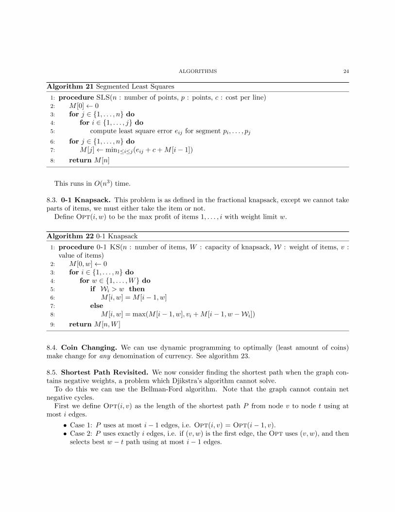
Algorithm 21 Segmented Least Squares

1: procedure SLS(n : number of points, p : points, c : cost per line)2: M [0] 03: for j 2 {1, . . . , n} do4: for i 2 {1, . . . , j} do5: compute least square error eij for segment pi, . . . , pj

6: for j 2 {1, . . . , n} do7: M [j] min1ij(eij + c+M [i� 1])

8: return M [n]

This runs in O(n3) time.

8.3. 0-1 Knapsack. This problem is as defined in the fractional knapsack, except we cannot takeparts of items, we must either take the item or not.

Define Opt(i, w) to be the max profit of items 1, . . . , i with weight limit w.

Algorithm 22 0-1 Knapsack

1: procedure 0-1 KS(n : number of items, W : capacity of knapsack, W : weight of items, v :value of items)

2: M [0, w] 03: for i 2 {1, . . . , n} do4: for w 2 {1, . . . ,W} do5: if Wi > w then6: M [i, w] = M [i� 1, w]7: else8: M [i, w] = max(M [i� 1, w], vi +M [i� 1, w �Wi])

9: return M [n,W ]

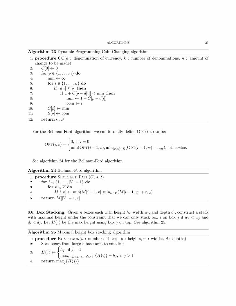
8.4. Coin Changing. We can use dynamic programming to optimally (least amount of coins)make change for any denomination of currency. See algorithm 23.

8.5. Shortest Path Revisited. We now consider finding the shortest path when the graph con-tains negative weights, a problem which Djikstra’s algorithm cannot solve.

To do this we can use the Bellman-Ford algorithm. Note that the graph cannot contain netnegative cycles.

First we define Opt(i, v) as the length of the shortest path P from node v to node t using atmost i edges.

• Case 1: P uses at most i� 1 edges, i.e. Opt(i, v) = Opt(i� 1, v).• Case 2: P uses exactly i edges, i.e. if (v, w) is the first edge, the Opt uses (v, w), and thenselects best w � t path using at most i� 1 edges.

ALGORITHMS 25

Algorithm 23 Dynamic Programming Coin Changing algorithm

1: procedure CC(d : denomination of currency, k : number of denominations, n : amount ofchange to be made)

2: C[0] 03: for p 2 {1, . . . , n} do4: min 15: for i 2 {1, . . . , k} do6: if d[i] p then7: if 1 + C[p� d[i]] < min then8: min 1 + C[p� d[i]]9: coin i

10: C[p] min11: S[p] coin

12: return C, S

For the Bellman-Ford algorithm, we can formally define Opt(i, v) to be:

Opt(i, v) =

(0, if i = 0

min(Opt(i� 1, v),min(v,w)2E(Opt(i� 1, w) + cvw), otherwise.

See algorithm 24 for the Bellman-Ford algorithm.

Algorithm 24 Bellman-Ford algorithm

1: procedure Shortest Path(G, s, t)2: for i 2 {1, . . . , |V |� 1} do3: for v 2 V do4: M [i, v] min(M [i� 1, v],minw2V (M [i� 1, w] + cvw)

5: return M [|V |� 1, s]

8.6. Box Stacking. Given n boxes each with height hi, width wi, and depth di, construct a stackwith maximal height under the constraint that we can only stack box i on box j if wi < wj anddi < dj . Let H(j) be the max height using box j on top. See algorithm 25.

Algorithm 25 Maximal height box stacking algorithm

1: procedure Box stack(n : number of boxes, h : heights, w : widths, d : depths)2: Sort boxes from largest base area to smallest

3: H(j) (hj , if j = 1

maxi<j, wi>wj , di>dj{H(i)}+ hj , if j > 1

4: return maxj{H(j)}

ALGORITHMS 26

To compute the maximum as descibed in the algorithm requires n2 operations, which makes thealgorithm run in O(n2).

9. Network Flow

Given a directed graph G = (V,E), where each edge e is associated with its capacity c(e) > 0.Two special nodes source s and sink t are given where s 6= t. We want to maximize the totalamount of flow from s to t subject to two constraints:

(1) Flow on edge e doesn’t exceed c(e);(2) For every node v 6= s and v 6= t, incoming flow is equal to outgoing flow.

9.1. Minimum Cut.

Definition 9.1. An s � t cut C = (S, T ) is a partition of GV such that s 2 S and t 2 T . Thecut-set of C is the set

(u, v) 2 E : u 2 S, v 2 T.

Note that if the edges in the cut-set of C are removed, |f | = 0.

Definition 9.2. The capacity of an s� t cut is defined by

c(S, T ) =X

(u,v)2(S⇥T )\Ecuv =

X(i,j)2E

cijdij ,

where dij = 1 if i 2 S and j 2 T , 0 otherwise.

The minimum s� t cut problem is to minimize c(S, T ), that is, to determine S and T such thatthe capacity of the S � T cut is minimal.

Theorem 9.3. In a flow network, the maximum amount of flow passing from the source to the

sink is equal to the minimum cut, i.e. the smallest total weight of the edges which if removed would

disconnect the source from the sink.

Definition 9.4. A residual graph provides a systematic way to search for forward-backward oper-ations in order to find the maximum flow.

Given a flow network G, and a flow f on G, we define the residual graph Gf of G with respectto f as follows:

• The node set of Gf is the same as that of G.• Each edge e = (u, v) of Gf is with a capacity of ce � f(e).• Each edge e0 = (v, u) of Gf is with a capacity of f(e)

Example 9.5. Given a flow network with unit capacity edges consisting of a directed graph G =(V,E), a source s 2 V , and a sink t 2 V , and ce = 1 for all e 2 E, and also a parameter k. The goalis to delete k edges so as to reduce the maximum s� t flow in G by as much as possible. In otherwords, find a set of edges F ✓ E so that |F | = k and the maximum s� t flow in G0 = (V,E�F ) isas small as possible subject to this. Give a polynomial time algorithm to solve this problem. Argue(prove) that your algorithm does in fact find the graph with the smallest maximum flow.

Algorithm 26 is bottlenecked by finding the minimum cut. We can use Nagamochi and Ibaraki’salgorithm which finds a minimum cut in O(|V ||E|+ |V |2 log |V |) [3].

ALGORITHMS 27

Algorithm 26 Delete k edges to minimize flow

1: procedure Reduce flow(G, k)2: Find the minimum cut (A,B) where s 2 A and t 2 B.3: E0 edges that go from A to B4: if |E0| � k then5: F any k edges in E0

6: else7: F all edges in E0[ any k � |E0| other edges in G

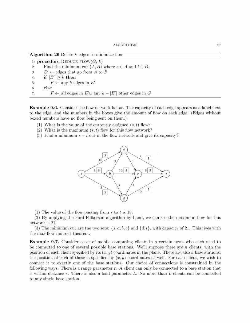
Example 9.6. Consider the flow network below. The capacity of each edge appears as a label nextto the edge, and the numbers in the boxes give the amount of flow on each edge. (Edges withoutboxed numbers have no flow being sent on them.)

(1) What is the value of the currently assigned (s, t) flow?(2) What is the maximum (s, t) flow for this flow network?(3) Find a minimum s� t cut in the flow network and give its capacity?

(1) The value of the flow passing from s to t is 18.(2) By applying the Ford-Fulkerson algorithm by hand, we can see the maximum flow for this

network is 21.(3) The minimum cut are the two sets: {s, a, b, c} and {d, t}, with capacity of 21. This jives with

the max-flow min-cut theorem.

Example 9.7. Consider a set of mobile computing clients in a certain town who each need tobe connected to one of several possible base stations. We’ll suppose there are n clients, with theposition of each client specified by its (x, y) coordinates in the plane. There are also k base stations;the position of each of these is specified by (x, y) coordinates as well. For each client, we wish toconnect it to exactly one of the base stations. Our choice of connections is constrained in thefollowing ways. There is a range parameter r. A client can only be connected to a base station thatis within distance r. There is also a load parameter L. No more than L clients can be connectedto any single base station.

ALGORITHMS 28

Your goal is to design a polynomial-time algorithm for the following problem. Given the positionsof a set of clients and a set of base stations, as well as the range and load parameters, decidewhether every client can be connected simultaneously to a base station, subject to the range andload conditions in the previous paragraph.

Algorithm 27 Check if all clients can connect to a base station

1: procedure Check all connect(C : clients, B : base stations, r, L)2: V source s [ C [ B [ sink t3: E edges with capacity 1 connecting s to all C, edges with capacity 1 connecting all C to

B if ci are close enough, and edges with capacity L from all B to t.4: G (V,E)5: f max-flow of G6: if f � |C| then7: return true8: else9: return false

In algorithm 27 the maximum number of clients that can connect is equal to the maximum flowvalue of the created graph. This algorithm is bottlenecked by the algorithm to find maximum flow,which if we use Ford-Fulkerson, is O(|E|f) where f is the maximum flow value.

10. Complexity Theory

Definition 10.1. P is the set of problems that can be solved in polynomial time.

Definition 10.2. NP is the set of problems that can be verified in polynomial time.

Definition 10.3. We can reduce a problem A to a problem B, by showing that solving B is thesame as solving A. This shows that problem B is at least as hard as problem A.

If we can reduce a problem to a known problem in P, then we know that that problem is also inP.

The shorthand for this idea of reduction is encapsulated in the symbol: P . Suppose we havetwo problems A and B, and B P A. Then we say that B is polynomial-time reducible to A. Italso implies that A is at least as hard as B since a solution to A is a solution to B.

Definition 10.4. A problem is in NP-complete if every problem in NP can be reduced to thatproblem. So an NP-complete problem is as hard as the hardest problem in NP.

Theorem 10.5. If problem A is in NP-complete and

(1) problem B is in NP

(2) A P B

then B is in NP-complete

ALGORITHMS 29

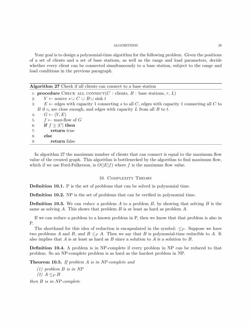
In other words, we can prove a new problem is NP-complete by reducing some other NP-completeproblem to it.

Figure 4. Diagram showing how P and NP are related in terms of complexity

Example 10.6. Prove that any language L such that L 2 NP can be decided by an algorithm thatruns in time 2O(nk), for some constant k.

Proof. Recall that for each language L in NP, there is an algorithm A that can verify each itemx 2 L in polynomial time, given a certificate y of length O(|x|c).

To establish if a given x 2 {0, 1}⇤ is in a given language L 2 NP, we determine if there is acertificate y of length O(|x|k), for some constant k, such that an accepting algorithm A can checkif A(x, y) = 1 or 0.

First we must determine if such a certificate y exists. To do this we need to test every y 2 {0, 1}⇤where |y| = O(|x|k) and evaluate A(x, y). Note that there are 2|y| possible certificates. If weevaluate A(x, y) with every possible y and the given x, then we will show if there exists a certificatey for which A(x, y) = 1.

Thus, we have shown that there exists an algorithm to decide if a language is in NP in 2O(nk). ⇤Example 10.7. You are give a directed graph G = (V,E) with weights we on its edges e 2 E.The weights can be negative or positive. The Zero-Weight Cycle Problem is to decide if there isa simple cycle in G so that that sum of the edge weights on this cycle is exactly 0. Prove thatZero-Weight Cycle is NP-Complete by reducing from the subset sum problem.

The Subset Sum Problem: Given natural numbers w1, w2, . . . , wn and a target number W , isthere a subset of {w1, w2, . . . , wn} that adds up to precisely W?

Proof. Suppose we are given a set of natural numbers {w1, w2, . . . , wn}. Let G be a directed graphwith n vertices, labeled 0, 1, . . . , n, and edges (i, j) for all pairs i < j. Let the weights of each edge(i, j) be wj . Also let there be edges (j, 0) of weight �W .

If there exists a subset H ✓ G such that the elements of H sum to W , then we define a cyclestarting at vertex 0, going through the vertices of H, and returning to 0 on an edge (j, 0). Theedges (j, 0) have weight �W which cancels the sum of all other edge weights in the cycle.

ALGORITHMS 30

If there exists a zero-weight cycle in G, then it must use the edge from (j, 0) and that weight�W must cancel all elements in the cycle. So excluding the edge (j, 0), all other edges in the cyclemust add up to W .

Thus, there is a subset of natural numbers that adds up to W if and only if G has a zero-weightcycle. Therefore, the subset sum problem p the zero-weight cycle problem. Since we know thesubset sum problem is in NP, it follows that the zero-weight cycle problem is in NP as well. ⇤Example 10.8. Suppose you’re helping to organize a summer sports camp, and the followingproblem comes up. The camp is supposed to have at least one counselor who is skilled at each ofthe n sports covered by the camp (baseball, volleyball, etc.). They have received job applicationsfrom m potential counselors. For each of the n sports, there is some subset of the m applicantsqualified in that sport. The question is: For a given number k < m, is it possible to hire at most kof the counselors and have at least one counselor qualified in each of the n sports? We’ll call thisthe E�cient Recruiting Problem. Show that E�cient Recruiting is NP-Complete.

The Vertex Cover Problem: Given a graph G and a number k, does G contain a vertex cover ofsize at most k? (Recall that a vertex cover V 0 ✓ V is a set of vertices such that every edge e 2 Ehas at least one of its endpoints in V 0.)

Proof. Suppose we are given a graph G and k 2 Z�0. Map each sport to an individual edge, andmap the counselors to an individual vertex. A counselor is qualified in sport if and only if thecorresponding edge goes to that counselor.

If there are k counselors who all together are qualified in all sports, then the vertices correspond-ing to those counselors have at least one edge that goes to them. Thus the counselor’s verticescreate a vertex cover of size k.

If there is a vertex cover of size k, then each counselor is qualified in at least one sport.Thus, G has a vertex cover of size at most k if and only if the we can be solve the e�cient

recruiting problem with at most k counselors. Therefore, the vertex cover problem p the e�cientrecruiting problem. Since we know the vertex cover problem to be in NP, it follows that the e�cientrecruiting problem must be in NP as well. ⇤

11. Approximation Algorithms

Approximation algorithms are an approach to determining solutions to computationally in-tractable problems. They run in polynomial time and find solutions that are guaranteed to beclose to optimal, yet are not guaranteed to be optimal.

References

[1] N. Touba, ‘Algorithms’, The University of Texas at Austin, 2016.[2] J. Kleinberg and E. Tardos, Algorithm design. Boston: Pearson/Addison-Wesley, 2006.[3] Computing Edge-Connectivity in Multigraphs and Capacitated Graphs, Hiroshi Nagamochi and Toshihide Ibaraki,

SIAM Journal on Discrete Mathematics 1992 5:1, 54-66