Algorithms and Complexity Results for Rail-Yard Routing

Negin Enayaty Ahangar1, Kelly M. Sullivan2, Shantih M. Spanton3, and Yu Wang3,4

1Naveen Jindal School of Management, University of Texas at Dallas, Richardson, TX,

USA, 750802Industrial Engineering Department, University of Arkansas, Fayetteville, AR, USA, 72701

3CSX Technology, Jacksonville, FL, USA, 322024JD Logistics, Beijing, China, 101111

July 8, 2019

Abstract

Rail yards are facilities that play a critical role in the freight rail transportation system. A number of

essential rail yard functions require moving connected “cuts” of rail cars through the rail yard from one

position to another. In a congested rail yard, it is therefore of interest to determine whether there exists

a feasible route for such a move and, if so, which one is shortest. With this motivation, we introduce the

yard-routing problem (YRP) and establish its fundamental theory. Two key features distinguish YRP

from a traditional shortest path problem: (i) the entity (i.e., the locomotive and attached cut of cars)

occupies space on the network; and (ii) track geometry further restricts route selection. To establish

the difficulty of solving YRP in general, we prove NP-completeness of a related problem that seeks to

determine whether there is space in the rail yard network to position the entity in a given direction

relative to a given anchor node. However, we then demonstrate this problem becomes polynomially

solvable—and therefore, YRP becomes polynomially solvable, too—for “bounded cycle length” (BCL)

yard networks, a practically important class of networks in which the yard topology will not allow the

entity to collide with itself. We formalize the resulting two-stage algorithm for BCL yard networks and

validate our algorithm on a rail yard data set provided by the class I railroad CSX Transportation.

Keywords: Rail-yard operations, shortest path, algorithms

1 Introduction

In the freight rail industry, rail cars are commonly carried across thousands of miles of track on several distinct

trains (a collection of locomotives and rail cars) before reaching their destination. Numerous rail yards dot

the physical rail network and act as sorting facilities, classifying rail cars by their final or intermediate

destination in order to assemble outbound trains from rail cars arriving via inbound trains and/or customer

shipment pickups.

Rail yard operations are critical to freight rail transportation but complex due to significant freight

volume and structural limitations on rail car movements. Figure 1 depicts a typical intermodal rail yard,

1

Figure 1: Track infrastructure at an intermodal rail yard. (This image is authorized for such use by CSXCorporation, Inc. Any person or organization not affiliated with or authorized by CSX may not use, copy,alter or modify any CSX photographs, graphics, videography or other, similar reproductions or recordingswithout the advance written permission of CSX.)

including the track infrastructure that enables (but restricts) car movements through the rail yard. Larger

rail yards, and/or rail yards that perform different functions, may have increased complexity. For instance,

Bailey Yard (in North Platte, Nebraska) is a classification yard that handles an average of 14, 000 rail cars

per day and occupies over 4 square miles of land area [15]. Despite the complexity, rail yard operations are

usually orchestrated by one or two yard officials overseeing multiple crews who manually execute instructions.

Rail yard operations depend on the ability to move cars through the rail yard. Connected cuts of cars are

moved with locomotives for many purposes including bringing the cars into the yard; collecting cars together

to go on an outbound train or to a customer; and moving cars to designated inspection, holding, and

maintenance areas. With the exception of the gravity-assisted presorting moves that occur at high-volume

hump yards, nearly all routing of cars in the yard is accomplished manually by individual locomotives at

the yard. Due to the high volume of manual handling moves, how these handling moves are routed has a

significant impact on the yard’s efficiency, including utilization of locomotives and throughput of cars. Our

research seeks to improve the efficiency of rail-yard operations by developing algorithms for routing a cut

of cars through a rail yard. In the short term, these algorithms can be incorporated into decision-support

systems to help yard officials better orchestrate yard operations. In the long term, these algorithms can be

used as a building block toward automating yard operations. The following paragraphs further detail our

motivation in the context of current yard operations planning procedures that are common in the freight

rail industry.

Currently, real-time operations are planned “intuitively” by yard personnel. Strategic planning can be

done with the assistance of specialized decision-support tools, including yard simulations that output key

efficiency metrics such as throughput volume, on-time departure of cars, handling frequency, and total time

in the yard. All but the most basic simulations incorporate routing cars through the yard. As routes must

be calculated tens of thousands of times in any simulation, calculation speed is imperative. Although the

2

details of these industry-used simulations remain unpublished, most simulations developed by several major

rail carriers of which the authors are aware route cars using simple shortest path, modified shortest path,

or pre-calculation of routes, often without considering the length of the cut of cars and locomotive; that is,

the entity is considered a point mass. In practice, the locomotive and cut occupy space on the track, which

can complicate routing decisions. Therefore, the existing routing techniques may fail when highly accurate

routes are required.

The current process of planning routes “intuitively” poses significant challenges, particularly when the

yard is congested and/or when multiple moves must be orchestrated simultaneously. With this motivation,

there is a movement toward the development of smart decision tools that can automate rail-yard operations,

including the planning and execution of routes. This movement further motivates our research to automate

route planning and execution for cases where a routing subroutine requires highly accurate routes.

In this paper we seek to optimize the route selection from among all possible routes in a rail yard subject

to the geometry of the yard network and the space occupied by the locomotive and cars. To the best of our

knowledge, this problem has not been studied in the literature.

In contrast to the micro-scale, yard-level routing problem we consider, the majority of rail-related routing

research focuses on line-of-road train movements between rail yards. The most researched line-of-road routing

problems include train design, timetabling, and real-time traffic management. Train design problems seek to

create a fixed, repeatable plan to handle all traffic on the network. These problems may include blocking [1, 4],

routing [5, 10, 16], route frequency [16], and scheduling [2] decisions and take on extraordinary complexity

when constraints of locomotive availability, crew restrictions, and maintenance (planned and unplanned) are

included. Timetabling problems [6, 7] aim to schedule trains along corridors having limited locations where

more than one track exists in parallel, providing the opportunity for one train to pass another. Taking

into account each train’s priority, length, speed, acceleration, and deceleration, timetabling problems seek to

determine when and where passes should occur. (It should be noted that trains are often too long to be held

in busy yards for the purpose of these passes so the passing must be done on the line of road.) Real-time

traffic management problems [8, 12, 13, 14] adjust routing plans under disturbance of the predetermined

routing plan, which can cause propagating delays.

In these common macro-scale, line-of-road routing problems, the infrastructure is primarily modeled as

a network of nodes, corresponding to rail yards, and edges, corresponding to corridors. The routing itself is

often modeled simply with the numerous operational constraints adding enough complexity amidst competing

objectives of customer satisfaction, cost reduction, and efficient asset utilization. By contrast, our yard-level

routing problem is posed over a network in which the edges correspond to individual tracks and the nodes

are track connections or switches. On this network, we seek to determine a shortest feasible route within the

rail yard for the locomotive and attached cut of cars (referred to as “entity” hereafter for brevity) subject to

the geometry of the yard tracks. This problem differs from a traditional shortest path problem in that the

route must (i) accommodate the entity’s physical length, (ii) avoid “prohibited” switch node traversals, and

(iii) satisfy restrictions on the entity’s orientation (i.e., which way the locomotive is facing) at arrival. We

consider two subproblems of this routing problem: a preprocessing stage that determines whether the yard

will accommodate the entity positioned with one of its endpoints at a given node; and a routing stage that

finds a shortest route given the output of the preprocessing stage.

Our main contributions are as follows: (i) we (in Section 2) define terminology and notation and (in

Section 3) introduce the yard-routing problem (YRP) to the academic literature; (ii) we (in Section 4) prove

3

1 2 3 4 5 6 7 8 9

10 11 13 1412 15 16 17 18 19 20 21 22

23 24 25 26 292827 30 31 32

36353433 37 38 41 424039 4443

2 2

2

2

2

1 1 3

2

4 1

1

2

41 1 2

11

1

18

1

2

5

1

2

2

1

2

3

2

3

1

33

12

3

2

1 2

2 8

9

2

1 4 42

9

2

8 4

idle cars idle cars

idle cars idle cars

idle cars

entity length, L = 6

locomotive endof origin position

locomotive endof destination position

Figure 2: Example yard network in which each edge e ∈ E is labeled with length ce and each node’s identifieri is labeled with a number attached to the node by a faint red vertical line. For convenience, nodes havebeen numbered in increasing order from left to right and top to bottom. Each switch node is drawn suchthat its acute angle appears as an acute angle. Dashed red lines are not to be interpreted as edges; rather,they indicate track segments that are unavailable because they are occupied by idle cars.

the preprocessing problem is NP-complete; (iii) we (in Section 4) develop a linear programming formulation

that solves an important special case of the preprocessing stage in polynomial time; (iv) given solutions to

each switch node’s preprocessing problem, we (in Section 5) demonstrate the special case from (iii) also leads

to polynomial-time solution of the routing stage and therefore a polynomial-time algorithm for the yard-

routing problem; (v) we (in Section 6) validate our model and algorithm on a rail yard data set provided

by the class I railroad CSX Transportation. Section 7 concludes the paper and discusses opportunities for

future research.

2 Yard Network Preliminaries

We consider the problem of routing an entity of length L ≥ 0 through a rail yard defined by the undirected

network G = (N,E) with nodes N and edges E. Figure 2 illustrates an example yard network. Edges in the

yard network correspond to track segments and nodes correspond to connections between track segments.

Commonly, there are idle cars in the rail yard that obstruct the entity’s movement. This feature can be

incorporated by removing occupied portions of edges from the network.

The entity consists of a locomotive that can either pull or push the attached cars. Let ce ≥ 0 denote the

length of edge e ∈ E, and let N(i) ⊆ N \ {i} denote the set of nodes adjacent to node i ∈ N . Number the

nodes adjacent to i ∈ N as N(i) = {Nk(i)}|N(i)|k=1 and the edges adjacent to i ∈ N as {e(i, k)}|N(i)|

k=1 where

e(i, k) ≡ [i,Nk(i)]. We refer to N1(i), N2(i), and N3(i) respectively as the first, second, and third neighbor of

node i and to {Nk(i)}|N(i)|k=1 as the ordered adjacency list of node i. The yard network G has special structure

as described below:

Property 1 |N(i)| ≤ 3, ∀i ∈ N . That is, each node has degree at most three.

In practice, there exist yard switches that split up to four ways; however, Property 1 is without loss of

generality because these switches can be modeled as two degree-three switches separated by an edge of

neglible length. We now formalize definitions that will enable analysis of yard networks.

4

N3(i)

i N1(i)

N2(i)

e(i, 3)

e(i, 2)

e(i, 1)

Figure 3: Schematic of a switch node i

Definition 1 If |N(i)| = 3, then i ∈ N is said to be a switch node. Define S ⊆ N as the set of switch nodes.

For a switch node i ∈ S, the collection of nodes {i,N1(i), N2(i), N3(i)} are always oriented (see Figure 3)

such that, among the three edges {e(i, k)}3k=1, exactly one pair of edges forms an acute angle. Without loss

of generality, suppose the edges e(i, 2) and e(i, 3) associated with each switch node i ∈ S form an acute angle.

By appropriately numbering the neighbors of each switch node, the following properties will be satisfied:

Property 2 For i ∈ N with |N(i)| ≥ 2, the edge pair {e(i, 1), e(i, 2)} is not an acute angle.

Property 3 For i ∈ S, the edge pair {e(i, 1), e(i, 3)} is not an acute angle.

Property 4 For i ∈ S, the edge pair {e(i, 2), e(i, 3)} is an acute angle.

When a network satisfies Properties 1–4, we say that the network has yard structure or is a yard network.

To illustrate Properties 1–4, examine switch node 3 in Figure 2. The edges [3, 4] and [3, 10] form an acute

angle; therefore, e(3, 1) is the edge [3, 2], e(3, 2) is either [3, 4] or [3, 10], and e(3, 3) is the remaining edge

adjacent to node 3. For a yard network satisfying Properties 1–4, we now present additional definitions

toward representing the entity’s positions in the yard network.

Definition 2 A sequence of edges e(1)–e(2)–· · · –e(m) is said to be a walk provided that each successive pair

of edges has exactly one endpoint in common. Alternatively, we may refer to the walk e(1)–e(2)–· · · –e(m)

by listing its nodes in sequence, e.g., as i(0)–i(1)–· · · –i(m).

For simplicity of exposition, we also assume the following without loss of generality.

Assumption 1 If e ∈ E and e′ ∈ E share two common endpoints, then e = e′.

Assumption 1 enables representing the length of an edge e = [i, j] ∈ E as either ce, cij , or cji. This assumption

is without loss of generality because dual edges of the form [i, j] can be “repaired” by replacing one of the

two edges with a new switch node i′, a new leaf node i′′, and edges {e(i, k)}3k=1 such that e(i′, 1) = [i′, i],

e(i′, 2) = [i′, j], and e(i′, 3) = [i′, i′′]. In this transformation, the new edge [i′, i′′] is assigned a length of zero

and edges [i′, i] and [i′, j] are each assigned a length equal to one-half of the replaced edge’s length.

Definition 3 A walk e(1)–e(2)–· · · –e(m) is said to be an acute-angle-free walk (abbreviated as “AAF walk”)

provided that none of its adjacent edge pairs are acute angles. For instance, 15–6–5–2–3–4–5 is an AAF walk

in Figure 2, but 3–4–5–2 is not because it traverses the acute angle {[4, 5], [5, 2]}.

Definition 4 An AAF walk e(1)–e(2)–· · · –e(m), with nodes i(0)–i(1)–· · · –i(m), is said to be closed if i(0) =

i(m) and {e(1), e(m)} is not an acute angle. Because Figure 2 does not contain any closed AAF walks, we

have illustrated two closed AAF walks in Figure 4.

5

(a)

1

2

3

4(b)

1

2

3 4

5

6

78

Figure 4: Illustration of closed AAF walks (a) 1–2–3–4–1 and (b) 3–2–1–8–3–4–5–6–7–4–3. In subfigure (b),note that 3–2–1–8–3 is not a closed AAF walk because {[2, 3], [3, 8]} is an acute angle.

Definition 5 An AAF walk i(0)–i(1)–· · · –i(m) is said to be a simple acute-angle-free walk (abbreviated as

“SAAF walk”) provided that (i) the walk visits i(m) no more than twice and (ii) the remaining |N | − 1

nodes are visited by the walk no more than once. (Thus, only one node may be visited twice by a SAAF

walk, and that node must be the last node on the walk.) For example, 15–6–5–2–3–4–5 is a SAAF walk in

Figure 2, but 15–6–5–2–3–4–5–6 is not due to the repetition of node 5.

Definition 6 An AAF walk (respectively, SAAF walk) W , with nodes i(0)–i(1)–· · · –i(m), is said to be an

“AAF(j) walk” (respectively, “SAAF(j) walk”) if j = i(0). The walk W is said to be an “AAF(i,j) walk”

(respectively, “SAAF(i,j) walk”) if i = i(0) and j = i(m). For example, 15–6–5–2–3–4–5 is at once an

AAF(15) walk, an AAF(15,5) walk, a SAAF(15) walk, and a SAAF(15,5) walk in Figure 2.

Definition 7 An AAF(j) walk (respectively, SAAF(j) walk) W , with nodes (j =) i(0)–i(1)–· · · –i(m), is

said to be positive anchored if i(1) = N1(j). In this case, we say W is an “AAF(j[+]) walk” (respectively,

“SAAF(j[+]) walk”). For example, 16–15–6–5–2–3–4–5 is a SAAF(16[+]) walk in Figure 2, but 16–29–30–

31–44–32 is not because N1(16) 6= 29 (i.e., edge [16, 29] is in node 16’s acute angle).

Definition 8 An AAF(j) walk (respectively, SAAF(j) walk) W , with nodes (j =) i(0)–i(1)–· · · –i(m), is

said to be negative anchored if i(1) ∈ {N2(j), N3(j)}. In this case, we say W is an “AAF(j[−]) walk”

(respectively, “SAAF(j[−]) walk”). For example, 16–29–30–31–44–32 is a SAAF(16[−]) walk in Figure 2.

Just as Definitions 7 and 8 classify an AAF(j) walk based upon whether its first edge leads to node

N1(j), we may similarly classify an AAF(i, j) walk on the basis of its first and last edge.

Definition 9 An AAF(i,j) walk (respectively, SAAF(i,j) walk) W , with nodes (i =) i(0)–i(1)–· · · –i(m) (=

j), is said to be an “AAF(i[+],j) walk” (respectively, “SAAF(i[+],j) walk”) if i(1) = N1(i) and an “AAF(i[−],j)

walk” (respectively, “SAAF(i[−],j) walk”) if i(1) ∈ {N2(i), N3(i)}. The walk W is said to be an “AAF(i,j[+])

walk” (respectively, “SAAF(i,j[+]) walk”) if i(m − 1) = N1(j) and an “AAF(i,j[−]) walk” (respectively,

“SAAF(i,j[−]) walk”) if i(m − 1) ∈ {N2(j), N3(j)}. For example, 37–36–23–10–3–2 is a SAAF(37[+],2[+])

walk in Figure 2 because N1(37) = 36 and N1(2) = 3; however, 37–36–23–10–3 is a SAAF(37[+],3[−]) walk

because 10 ∈ {N2(3), N3(3)}.

There definitions above will be useful in characterizing the entity’s movement through the yard, as we

now summarize. To traverse the edge pair {e(j, 2), e(j, 3)}, j ∈ S, in sequence, the entity’s entire length must

first pass through node j before it reverses its direction to continue with the intended walk. For example,

suppose we wish to move the entity from its original position in Figure 2 along a walk beginning 21–22–32–31

6

1 2 3 4 5 6 7 8 9

10 11 13 1412 15 16 17 18 19 20 21 22

23 24 25 26 292827 30 31 32

36353433 37 38 41 424039 4443

2 2

2

2

2

1 1 3

2

4 1

1

2

41 1 2

11

1

18

1

2

5

1

2

2

1

2

3

2

3

1

33

12

3

2

1 2

2 8

9

2

1 4 42

9

2

8 4

locomotive endof origin position

(Step 0)

locomotive endof position(Step 1)

locomotive endof position(Step 2)

Figure 5: Illustration of a subnetwork of Figure 2 in which the entity traverses the acute angle at node 22.

(using the acute angle at node 22) toward the destination position. As illustrated in Figure 5, the entire

entity must pass node 22 and continue on to the SAAF(22[+]) walk 22–8–9 before traversing 22–32–31.

As a result of the discussion in the previous paragraph, a necessary condition to traverse the acute angle

{e(j, 2), e(j, 3)}, j ∈ S, is the existence of a SAAF(j[+]) walk of length at least L (hereafter referred to as a

“SAAF(j[+]) feasible position”). In this case, we say the the acute angle {e(j, 2), e(j, 3)} is feasible. These

definitions are formalized below.

Definition 10 A SAAF walk e(1)–e(2)–· · · –e(m) (with node representation i(0)–i(1)–· · · –i(m)) is said to

be a feasible position for the entity if ce(1) + ce(2) + · · · + ce(m) ≥ L. For instance, 20–21–22 is illustrated

as the entity’s original feasible position, where L = 6. If j = i(0) ∈ S and N1(j) = i(1), then we say the

feasible position is positive anchored at j or that the feasible position is a “SAAF(j[+]) feasible position.”

For example, 20–21–22 is not a SAAF(20[+]) feasible position in Figure 2 because N1(20) 6= 21.

Definition 11 If there exists a SAAF(j[+]) feasible position, the acute angle {e(j, 2), e(j, 3)} is said to be a

feasible acute angle; otherwise, {e(j, 2), e(j, 3)} is said to be an infeasible acute angle.

Corresponding to the problem of determining the feasibility of acute angle at switch node j ∈ S, it is of

interest to identify SAAF(j[+]) and SAAF(j[−]) walks of maximum length. We therefore make the following

additional definition.

Definition 12 Let γj and γj respectively denote the length of the longest SAAF(j[+]) walk and the length

of the longest SAAF(j[−]) walk. For example, γ4 = 27 corresponding to the SAAF(4[+]) walk 4–5–6–15–16–

29–30–31–44–32–22–8–9 in Figure 2, and γ31 = 18 corresponding to the SAAF(31[−]) walk 31–44–32–22–8–9.

7

jh jh+1

A

B

Wh−1

Wh

Wh+1

· · ·

LL/2

LL/2

Figure 6: Illustration of entity traversing walk Wh (highlighted in green) for h ∈ {1, . . . ,H−1}. In traversingthe acute angles at nodes jh and jh+1, the entity (colored blue) respectively moves until its midpoint haspassed jh and jh+1 by a distance of L/2 units (to points marked by “A” and “B”).

For now, we have neglected the computational effort required to compute γj and γj . We will address

this subject in further detail in Section 4.

3 Problem Definition and Overview of Approach

In this section, we characterize how the entity moves inside the rail yard and formally define the YRP,

which (informally) seeks to determine how the entity should move from a specified origin feasible position

to a specified destination feasible position in order to minimize the total distance traveled by the entity.

For simplicity of exposition, we assume the origin and destination are nodes f ∈ N and g ∈ N (e.g.,

f = 21 and g = 34 in Figure 2), which can be interpreted as the initial and final location of the entity’s

midpoint. For the cases of this problem that we show to be polynomially solvable, we show (in Remark 3

of Section 5) it is possible to transform a problem with origin/destination feasible positions into a problem

with origin/destination nodes, so this assumption poses no additional loss of generality.

By definition, the entity must travel on an AAF walk between consecutive traversals of acute angles.

Therefore, if the entity traverses H acute angles (at switch nodes j1, j2, . . . , jH , numbered in the order of

traversal) on its route from f to g, the route can be described by a sequence of AAF walks W 0,W 1, . . . ,WH

that satisfy the following conditions.

Condition 1 If H ≥ 1, W 0 is an AAF(f ,j1[−]) walk; otherwise W 0 is an AAF(f ,g) walk.

Condition 2 For all h ∈ {1, . . . ,H − 1}, Wh is an AAF(jh[−],jh+1[−] ) walk.

Condition 3 If H ≥ 1, WH is an AAF(jH[−],g) walk.

Condition 4 For all h ∈ {1, . . . ,H}, there exists a SAAF(jh[+]) feasible position Wh. (That is, the traversed

acute angles are, in fact, feasible.)

Concerning Wh, h ∈ {0, . . . ,H}, let the statement “the entity traverses Wh” indicate that the entity’s

midpoint begins L/2 distance units into Wh, moves to jh along Wh (in reverse direction), moves from jh to

jh+1 along Wh, and then moves L/2 distance units into Wh+1. This movement is illustrated in Figure 6.

The entity’s orientation may further constrain the route selection: For instance, if the destination node

is on a chain of nodes that leads to a leaf node, the locomotive must push the cars in backward onto the

track, so as not to trap itself on the track behind the cars. Towards enforcing orientation restrictions on

8

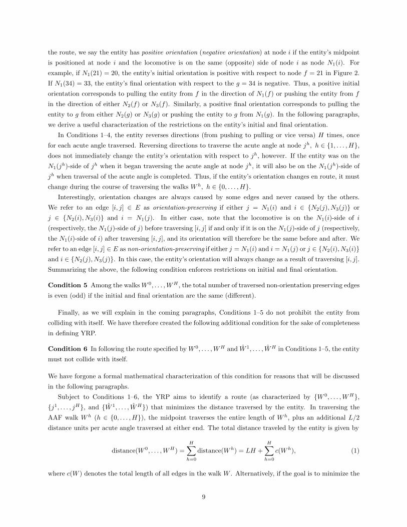
the route, we say the entity has positive orientation (negative orientation) at node i if the entity’s midpoint

is positioned at node i and the locomotive is on the same (opposite) side of node i as node N1(i). For

example, if N1(21) = 20, the entity’s initial orientation is positive with respect to node f = 21 in Figure 2.

If N1(34) = 33, the entity’s final orientation with respect to the g = 34 is negative. Thus, a positive initial

orientation corresponds to pulling the entity from f in the direction of N1(f) or pushing the entity from f

in the direction of either N2(f) or N3(f). Similarly, a positive final orientation corresponds to pulling the

entity to g from either N2(g) or N3(g) or pushing the entity to g from N1(g). In the following paragraphs,

we derive a useful characterization of the restrictions on the entity’s initial and final orientation.

In Conditions 1–4, the entity reverses directions (from pushing to pulling or vice versa) H times, once

for each acute angle traversed. Reversing directions to traverse the acute angle at node jh, h ∈ {1, . . . ,H},does not immediately change the entity’s orientation with respect to jh, however. If the entity was on the

N1(jh)-side of jh when it began traversing the acute angle at node jh, it will also be on the N1(jh)-side of

jh when traversal of the acute angle is completed. Thus, if the entity’s orientation changes en route, it must

change during the course of traversing the walks Wh, h ∈ {0, . . . ,H}.Interestingly, orientation changes are always caused by some edges and never caused by the others.

We refer to an edge [i, j] ∈ E as orientation-preserving if either j = N1(i) and i ∈ {N2(j), N3(j)} or

j ∈ {N2(i), N3(i)} and i = N1(j). In either case, note that the locomotive is on the N1(i)-side of i

(respectively, the N1(j)-side of j) before traversing [i, j] if and only if it is on the N1(j)-side of j (respectively,

the N1(i)-side of i) after traversing [i, j], and its orientation will therefore be the same before and after. We

refer to an edge [i, j] ∈ E as non-orientation-preserving if either j = N1(i) and i = N1(j) or j ∈ {N2(i), N3(i)}and i ∈ {N2(j), N3(j)}. In this case, the entity’s orientation will always change as a result of traversing [i, j].

Summarizing the above, the following condition enforces restrictions on initial and final orientation.

Condition 5 Among the walks W 0, . . . ,WH , the total number of traversed non-orientation preserving edges

is even (odd) if the initial and final orientation are the same (different).

Finally, as we will explain in the coming paragraphs, Conditions 1–5 do not prohibit the entity from

colliding with itself. We have therefore created the following additional condition for the sake of completeness

in defining YRP.

Condition 6 In following the route specified by W 0, . . . ,WH and W 1, . . . , WH in Conditions 1–5, the entity

must not collide with itself.

We have forgone a formal mathematical characterization of this condition for reasons that will be discussed

in the following paragraphs.

Subject to Conditions 1–6, the YRP aims to identify a route (as characterized by {W 0, . . . ,WH},{j1, . . . , jH}, and {W 1, . . . , WH}) that minimizes the distance traversed by the entity. In traversing the

AAF walk Wh (h ∈ {0, . . . ,H}), the midpoint traverses the entire length of Wh, plus an additional L/2

distance units per acute angle traversed at either end. The total distance traveled by the entity is given by

distance(W 0, . . . ,WH) =

H∑h=0

distance(Wh) = LH +

H∑h=0

c(Wh), (1)

where c(W ) denotes the total length of all edges in the walk W . Alternatively, if the goal is to minimize the

9

time taken to complete the route, L and ce, e ∈ E, could be replaced in Equation (1) by an estimate of the

time to traverse an acute angle and the time to traverse edge e.

Given the need for rail providers to solve YRP quickly and repeatedly, our research seeks to identify

cases under which YRP can be solved efficiently. Towards this end, a logical approach is to subdivide the

routing problem into two stages: (i) a preprocessing stage that determines whether each switch node’s acute

angle is feasible and (ii) a routing stage that finds a shortest f -g walk that prohibits infeasible acute angles,

penalizes feasible acute angles, and enforces orientation restrictions at f and g. For instance, if L = 6 in

Figure 5, the preprocessing stage would identify that (among others) the acute angles at nodes 22 and 35

are feasible (e.g., due to the SAAF(22[+]) walk 22–8–9 and the SAAF(35[+]) walk 35–36–37–24–25–26). The

routing stage would then determine that these two acute angles would be traversed in sequence (i.e., j1 = 22

and j2 = 35) and that the AAF walks W 0 (21–22), W 2 (22–32–31–30–29–28–41–40–35), and W 3 (35–34)

would connect these acute angles to the origin node f = 21 and destination node g = 34. In this case, note

that it would not have been sufficient for the entity to proceed directly to the destination node g = 34 along

an AAF walk after traversing the acute angle at node 22; doing so would have resulted in a violation of

Condition 5 and thus, the entity would have an incorrect final orientation.

As we will demonstrate, the viability of our two-stage approach depends on the presence (or absence) of

SAAF walks from a node to itself, and on the length of such walks. To formalize these conditions, we make

the following additional definition.

Definition 13 A SAAF walk i(0)–i(1)–· · · –i(m) is said to be an acute-angle-free cycle (abbreviated “AAF

cycle”) if i(0) = i(m). For instance, 5–4–3–2–5 is at once a SAAF(5[−]) walk and an AAF cycle in Figure 2;

however, it is not a closed AAF walk because {[5, 4], [2, 5]} is an acute angle.

In fact, the two-stage approach yields a polynomial algorithm for YRP under networks, which we refer to

hereafter as “bounded cycle length” or “BCL,” that satisfy the following assumption.

Assumption 2 All AAF cycles in the yard network have length at least L.

Assumption 2 simplifies YRP in a couple of meaningful ways. Because the entity must always occupy an

edge subset that forms a feasible position, Condition 6 is automatically satisfied by enforcing that any SAAF

walk that begins and ends with the same node is longer than the entity itself; thus, the two-stage solution

approach is valid, where the preprocessing stage evaluates all acute angles for feasibility and Conditions 1–5

are then addressed in the routing stage—in the vein of a “shortest path with turn penalties” problem—by

reformulating YRP as a traditional shortest path problem on an expanded directed network. It is important

to note that Assumption 2 can be verified in polynomial time using an extension of classical shortest path

algorithms. We explain in detail in Remark 2 of Section 4.3.

When Assumption 2 is not satisfied (i.e., for non-BCL networks), the two-stage approach fails altogether.

(For instance, the SAAF(jh[+]) feasible position Wh (h ∈ {1, . . . ,H}) may intersect the route leading into or

away from node j, or the AAF walk Wh (h ∈ {0, . . . ,H}) may include AAF cycles. In either of these cases,

an entity of sufficient length would collide with itself.) As justification of the difficulty in solving the general

YRP (i.e., on possibly non-BCL networks), we prove (in Section 4) NP-completeness of the preprocessing

problem. Because the preprocessing problem must be solved in order to determine a potential YRP route’s

feasibility, this result further implies that YRP is itself NP-hard but not contained in NP.

10

In addition to the theoretical contributions described above, we now argue that our two-stage algorithm

constitutes a significant practical contribution even though it will not handle non-BCL networks. Our

reasoning follows:

(i) In practice, it is common to move both short entities (i.e., those of length no more than L) and long

entities (those of length greater than L). In moving short entities, as is common in smaller yards

where numerous cuts of cars must be moved to assemble trains, Assumption 2 holds and YRP can be

solved in polynomial time. Although Assumption 2 does not hold for long entities, these moves tend

to be limited to specific yard functions performed in a dedicated portion of the yard that was designed

for the function. (For instance, a lengthy inbounded train enters the yard and is placed onto one or

more dedicated receiving tracks.) These moves will have a small number (usually just one) of potential

routes and therefore require little to no planning.

(ii) The structure of an incoming or outgoing lead which fans out into many other tracks to sort and hold

cars is typical of many rail yards, including the one depicted in Figure 1. Such yards are devoid of

AAF cycles and are therefore BCL.

(ii) Although we cannot guarantee it, the BCL algorithm may provide a building block for solving YRP

on non-BCL networks, as we discuss in Section 7.

Section 4 provides analysis and algorithms for the preprocessing stage, and Section 5 provides the routing

algorithm for BCL networks.

4 Preprocessing Stage

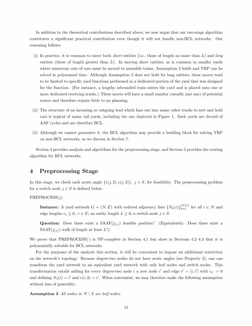
In this stage, we check each acute angle {e(j, 2), e(j, 3)}, j ∈ S, for feasibility. The preprocessing problem

for a switch node j ∈ S is defined below.

PREPROCESS(j)

Instance: A yard network G = (N,E) with ordered adjacency lists {Nk(i)}|N(i)|k=1 for all i ∈ N and

edge lengths ce ≥ 0, e ∈ E; an entity length L ≥ 0; a switch node j ∈ S.

Question: Does there exist a SAAF(j[+]) feasible position? (Equivalently: Does there exist a

SAAF(j[+]) walk of length at least L?)

We prove that PREPROCESS(·) is NP-complete in Section 4.1 but show in Sections 4.2–4.3 that it is

polynomially solvable for BCL networks.

For the purposes of the analysis this section, it will be convenient to impose an additional restriction

on the network’s topology. Because degree-two nodes do not have acute angles (see Property 2), one can

transform the yard network to an equivalent yard network with only leaf nodes and switch nodes. This

transformation entails adding for every degree-two node i a new node i′ and edge e′ = [i, i′] with ce′ = 0

and defining N3(i) = i′ and e(i, 3) = e′. When convenient, we may therefore make the following assumption

without loss of generality.

Assumption 3 All nodes in N \ S are leaf nodes.

11

s t

sss3

s2

t t0 t1 t2 t3 t411110 1

N

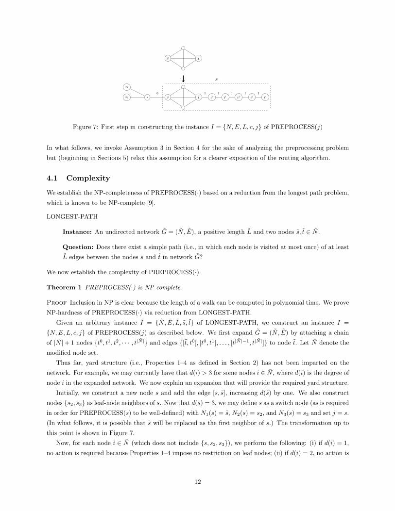
Figure 7: First step in constructing the instance I = {N,E,L, c, j} of PREPROCESS(j)

In what follows, we invoke Assumption 3 in Section 4 for the sake of analyzing the preprocessing problem

but (beginning in Sections 5) relax this assumption for a clearer exposition of the routing algorithm.

4.1 Complexity

We establish the NP-completeness of PREPROCESS(·) based on a reduction from the longest path problem,

which is known to be NP-complete [9].

LONGEST-PATH

Instance: An undirected network G = (N , E), a positive length L and two nodes s, t ∈ N .

Question: Does there exist a simple path (i.e., in which each node is visited at most once) of at least

L edges between the nodes s and t in network G?

We now establish the complexity of PREPROCESS(·).

Theorem 1 PREPROCESS(·) is NP-complete.

Proof Inclusion in NP is clear because the length of a walk can be computed in polynomial time. We prove

NP-hardness of PREPROCESS(·) via reduction from LONGEST-PATH.

Given an arbitrary instance I = {N , E, L, s, t} of LONGEST-PATH, we construct an instance I =

{N,E,L, c, j} of PREPROCESS(j) as described below. We first expand G = (N , E) by attaching a chain

of |N |+ 1 nodes {t0, t1, t2, · · · , t|N |} and edges {[t, t0], [t0, t1], . . . , [t|N |−1, t|N |]} to node t. Let N denote the

modified node set.

Thus far, yard structure (i.e., Properties 1–4 as defined in Section 2) has not been imparted on the

network. For example, we may currently have that d(i) > 3 for some nodes i ∈ N , where d(i) is the degree of

node i in the expanded network. We now explain an expansion that will provide the required yard structure.

Initially, we construct a new node s and add the edge [s, s], increasing d(s) by one. We also construct

nodes {s2, s3} as leaf-node neighbors of s. Now that d(s) = 3, we may define s as a switch node (as is required

in order for PREPROCESS(s) to be well-defined) with N1(s) = s, N2(s) = s2, and N3(s) = s3 and set j = s.

(In what follows, it is possible that s will be replaced as the first neighbor of s.) The transformation up to

this point is shown in Figure 7.

Now, for each node i ∈ N (which does not include {s, s2, s3}), we perform the following: (i) if d(i) = 1,

no action is required because Properties 1–4 impose no restriction on leaf nodes; (ii) if d(i) = 2, no action is

12

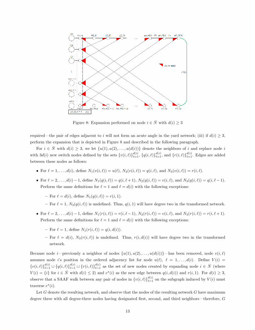
Figure 8: Expansion performed on node i ∈ N with d(i) ≥ 3

required—the pair of edges adjacent to i will not form an acute angle in the yard network; (iii) if d(i) ≥ 3,

perform the expansion that is depicted in Figure 8 and described in the following paragraph.

For i ∈ N with d(i) ≥ 3, we let {u(1), u(2), . . . , u(d(i))} denote the neighbors of i and replace node i

with 3d(i) new switch nodes defined by the sets {v(i, `)}d(i)`=1, {q(i, `)}d(i)

`=1, and {r(i, `)}d(i)`=1. Edges are added

between these nodes as follows:

• For ` = 1, . . . , d(i), define N1(v(i, `)) = u(`), N2(v(i, `)) = q(i, `), and N3(v(i, `)) = r(i, `).

• For ` = 2, . . . , d(i)− 1, define N1(q(i, `)) = q(i, `+ 1), N2(q(i, `)) = v(i, `), and N3(q(i, `)) = q(i, `− 1).

Perform the same definitions for ` = 1 and ` = d(i) with the following exceptions:

– For ` = d(i), define N1(q(i, `)) = r(i, 1).

– For ` = 1, N3(q(i, `)) is undefined. Thus, q(i, 1) will have degree two in the transformed network.

• For ` = 2, . . . , d(i)− 1, define N1(r(i, `)) = r(i, `− 1), N2(r(i, `)) = v(i, `), and N3(r(i, `)) = r(i, `+ 1).

Perform the same definitions for ` = 1 and ` = d(i) with the following exceptions:

– For ` = 1, define N1(r(i, `)) = q(i, d(i)).

– For ` = d(i), N3(r(i, `)) is undefined. Thus, r(i, d(i)) will have degree two in the transformed

network.

Because node i—previously a neighbor of nodes {u(1), u(2), . . . , u(d(i))}—has been removed, node v(i, `)

assumes node i’s position in the ordered adjacency list for node u(`), ` = 1, . . . , d(i). Define V (i) =

{v(i, `)}d(i)`=1 ∪ {q(i, `)}

d(i)`=1 ∪ {r(i, `)}

d(i)`=1 as the set of new nodes created by expanding node i ∈ N (where

V (i) = {i} for i ∈ N with d(i) ≤ 2) and e?(i) as the new edge between q(i, d(i)) and r(i, 1). For d(i) ≥ 3,

observe that a SAAF walk between any pair of nodes in {v(i, `)}d(i)`=1 on the subgraph induced by V (i) must

traverse e?(i).

Let G denote the resulting network, and observe that the nodes of the resulting network G have maximum

degree three with all degree-three nodes having designated first, second, and third neighbors—therefore, G

13

constitutes a yard network. Let N and E respectively denote the nodes and edges of this network, and

define S as the set of degree-three nodes. The node sets V (i), i ∈ N are disjoint, and only s, s2, and s3 are

contained within N but not⋃i∈N V (i).

We assign the length of edge e ∈ E as ce = 0 if (i) there exists a node i ∈ N such that both of the

endpoints of E are elements of V (i) or (ii) one of the endpoints of e is the node s; otherwise, ce = 1. In

particular, note that for each t`, ` = 1, . . . , |N |, the edge [t`−1, t`] is contained in E with unit length.

We now prove that the answer to PREPROCESS(s) for an entity of length L = L + |N | + 1 is “yes” if

and only if the answer to LONGEST-PATH is “yes.” Suppose there exists a SAAF(s[+]) feasible position

in G. Note that this position intersects a sequence of node sets V (i(0))–V (i(1))–· · · –V (i(m)), where i(h) ∈N , ∀h ∈ {0, 1, . . . ,m} and [i(h − 1), i(h)] ∈ E, ∀h ∈ {1, . . . ,m}, and i(0) = s based on the construction of

G. The length of this walk from the switch node s until it intersects V (i(0)) = V (s) is zero. For a given

h ∈ {0, 1, . . . ,m}, the walk may pass through several edges whose endpoints are both in V (i(h)); however,

the combined length of all such edges is zero. The walk also traverses m unit-length edges in moving from

V (i(h− 1)) to V (i(h)) for all h = 1, . . . ,m, and the total length of the walk is therefore

m ≥ L (= L+ |N |+ 1). (2)

Because each SAAF walk that enters and exits V (i), i ∈ N , must traverse e?(i), it is therefore impossible

to enter and exit V (i) a second time. Because each V (i), i ∈ N , may be exited at most once, the nodes

{i(0), i(1), . . . , i(m − 1)} are unique. Combining this observation with Equation (2), the maximum length

of any SAAF(s[+]) walk would be upper-bounded by |N | if the chain t0–t1–· · · –t|N | were excluded from E.

Because m > |N |, the set {i(0), i(1), . . . , i(m)} must include nodes in the chain. Furthermore, a SAAF

walk that enters the chain cannot leave the chain, and therefore i(m) ∈ {t0, t1, . . . , t|N |}. Without loss of

generality, we assume that i(m) = t|N |, extending the feasible position if necessary so that it includes all

nodes and edges in the chain. Summarizing the above, we have identified a feasible position that satisfies

i(h) = t|N |−m+h, h ∈ {m− |N |,m− |N |+ 1, . . . ,m}. Because [i(h− 1), i(h)] ∈ E, ∀h ∈ {1, . . . ,m}, we have

that (s =) i(0)–i(1)–· · · –i(m− |N | − 1) (= t) is an s-t path in G of length m− |N | − 1, which is at least L

by Equation (2). The answer to LONGEST-PATH is therefore “yes.”

Conversely, suppose there exists an s-t path (s =) i(0)–i(1)–· · · –i(h) (= t) of h ≥ L edges in G. Based

on construction of G, there is a SAAF(s[+]) walk in G with length h that traverses the node sets V (i(0))–

V (i(1))–· · · –V (i(h)). Noting that i(h) = t and the SAAF(s[+]) walk has not yet traversed any nodes in the

chain, we may extend this walk to obtain the SAAF(s[+]) walk V (i(0))–V (i(1))–· · · –V (i(h))–V (t0)–V (t1)–

· · · –V (t|N |), which has length h + N + 1 ≥ L + N + 1 = L. Therefore, the answer to PREPROCESS(s) is

“yes” and the proof of this theorem is complete. �

This proof establishes NP-completeness for the general case of PREPROCESS(·). The reduction, however,

yields yard networks with zero-length AAF cycles, which do not appear in practice. Indeed, as we summarize

in Sections 4.2–4.3, PREPROCESS(·) becomes polynomially solvable for BCL networks in which all AAF

cycles must have length at least L. Towards analyzing these cases, it will be useful to define two subroutines

that contract the network in a way that preserves both yard structure and Assumptions 3–2.

14

(a)1 2 3 4

10 8 7 5

9 6

1 5 3

2 2

1.5 1.5

2 2

(b)3 4

10 8 7 5

9 6

3

7 2

1.5 1.5

2 2

(c)42 43

10 8 7 5

9 6

10 5

1.5 1.5

2 2

Figure 9: (a) Notional yard network; (b) Resulting yard network after applying CONTRACT-2(1); (c)Resulting yard network after applying CONTRACT-1(4) to the yard network from (b).

CONTRACT-1(i)

Given: A leaf node i that is the first neighbor of switch node i′ ∈ S, i.e., i = N1(i′) and e(i′, 1) = [i, i′].

Procedure: Remove the leaf node i, the switch node i′, and all edges adjacent to i′. For k ∈ {2, 3},add a new leaf node ik and a new edge [Nk(i′), ik] with length ce(i′,1) + ce(i′,k). Let ik, k ∈ {2, 3}replace i′ in the ordered adjacency list of node Nk(i′).

CONTRACT-2(i)

Given: A leaf node i that is the second or third neighbor of switch node i′ ∈ S, i.e., i = Nk(i′) and

e(i′, k) = [i, i′] for some k ∈ {2, 3}. Let k′ denote the (unique) element of {2, 3} \ {k}.

Procedure: Remove the leaf node i, the switch node i′, and all edges adjacent to i′. Add a new

edge [N1(i′), Nk′(i′)] with length ce(i′,1) + ce(i′,k′). Let N1(i′) and Nk′(i

′) respectively replace i′ in the

ordered adjacency list of nodes Nk′(i′) and N1(i′).

Figure 9 illustrates the yard network that results upon executing CONTRACT-2(1) and CONTRACT-

1(4) in sequence. We now state an additional definition required in order to prove (in Lemmas 1–3) funda-

mental properties of these subroutines.

Definition 14 A SAAF(j[+]) (respectively, SAAF(j[−])) walk (j =) i(0)–i(1)–· · · –i(m) is said to be max-

imal if there does not exist a node j′ ∈ N such that i(0)–i(1)–· · · –i(m)–j′ is a SAAF(j[+]) (respectively,

SAAF(j[−])) walk. For example, 16–15–6–5–2–3–4–5 and 16–29–30–18 are respectively maximal SAAF(16[+])

and maximal SAAF(16[−]) walks in Figure 2; however, 16–15–6–5 is not a maximal SAAF(16[+]) walk because

it can be extended as 16–15–6–5–4 or 16–15–6–5–2 into another SAAF(16[+]) walk.

Lemma 1 Let i be any leaf node such that N1(i′) = i for some switch node i′ ∈ S. Let j ∈ S \ {i′}, and let

G′ denote the network that results upon executing CONTRACT-1(i). Then, (a) the maximum length among

all SAAF(j[+]) walks is the same in G and G′, and (b) the maximum length among all SAAF(j[−]) walks is

the same in G and G′.

15

Proof We prove part (a) by establishing that there exists a maximal SAAF(j[+]) walk of length l in G if

(←) and only if (→) there exists a maximal SAAF(j[+]) walk of length l in G′. Because ce ≥ 0, ∀e ∈ E,

there is always a maximal SAAF(j[+]) walk among the set of maximum-length SAAF(j[+]) walks, and this

will therefore establish the result.

Proof of (→): Let W , with nodes (j =) i(0)–i(1)–· · · –i(m), be a maximal SAAF(j[+]) walk of length l in

G. If W includes node i′, then (because W is maximal) W must also include i, and we therefore have the

following two cases: (I) W includes both node i′ and node i; and (II) W includes neither node i′ nor node i.

Proof of (→, Case I): Suppose W includes both node i and i′. Because i is a leaf node, we may assume

i(m) = i, i(m − 1) = i′, and i(m − 2) = Nk(i′) for some k ∈ {2, 3}. Because W is a SAAF walk, only

its last node may be repeated; therefore, i′ must be distinct from i(0), i(1), . . . , i(m − 2). Therefore, after

CONTRACT-1(i), the sub-walk (j =) i(0)–i(1)–· · · –i(m − 2) (= Nk(i′)) remains a SAAF(j[+]) walk in G′

and its length is l − ce(i′,k) − ce(i′,1) in both G and G′. Observe that CONTRACT-1(i) has inserted in G′

the new leaf node ik and the new edge [Nk(i′), ik] with length ce(i′,k) + ce(i′,1); thus, i(0)–i(1)–· · · –i(m− 2)

can be extended in G′ to i(0)–i(1)–· · · –i(m − 2)–ik, a SAAF(j[+]) walk with length l − ce(i′,k) − ce(i′,1) +

(ce(i′,k) + ce(i′,1)) = l. Because ik is a leaf node, this walk is maximal in G′ and case I is proved.

Proof of (→, Case II): Suppose W includes neither node i nor node i′. Note that all edges removed by

CONTRACT-1(i) were incident to node i′. Therefore, i(0)–i(1)–· · · –i(m) remains a SAAF(j[+]) walk in G′,

and its length remains l. Furthermore, if i′ is adjacent to i(m), it must be the case that [i(m − 1), i(m)]

and [i(m), i′] form an acute angle. Therefore, if CONTRACT-1(i) added any new edges that are adjacent

to i(m), that edge will also form an acute angle with [i(m− 1), i(m)]. Consequently, W remains maximal in

G′, thus completing the proof of this direction.

Proof of (←): Let W , with nodes (j =) i(0)–i(1)–· · · –i(m), be a maximal SAAF(j[+]) walk of length l

in G′. We prove that G contains a maximal SAAF(j[+]) walk of length l in two cases: (I) W includes either

node i2 or node i3; and (II) W includes neither node i2 nor i3.

Proof of (←, Case I): Suppose without loss of generality that W includes the new node i2 added in

CONTRACT-1(i). (The proof is symmetric if i2 is replaced by i3.) In G′, i2 is adjacent only to node N2(i′).

Because i2 is a leaf node in G′, W must also include node N2(i′) such that i(m− 1) = N2(i′) and i(m) = i2.

Removing i(m) from W yields the SAAF(j[+]) walk (j =) i(0)–i(1)–· · · –i(m − 1), which is contained in

both G′ and G and has length l − ce(i′,1) − ce(i′,2). In G, node i′ occupies the same position in the ordered

adjacency list of node N2(i′) as did node i2 in G′; therefore, because i′ is not in G′ (and is therefore distinct

from i(0), i(1), . . . , i(m− 1)), (j =) i(0)–i(1)–· · · –i(m− 1)–i′ is a SAAF(j[+]) walk of length l− ce(i′,1) in G.

Similarly, i 6= i′ is not in G′ and we therefore have that (j =) i(0)–i(1)–· · · –i(m − 1)–i′–i is a SAAF(j[+])

walk of length l, which is also maximal because i is a leaf node. This completes the proof of this case.

Proof of (←, Case II): Suppose W includes neither node i2 nor i3. Note that all edges removed by

CONTRACT-1(i) were incident to node i′. Therefore, i(0)–i(1)–· · · –i(m) remains a SAAF(j[+]) walk in G,

and its length remains l.

The proof of part (b) is identical to part (a) after replacing “SAAF(j[+])” throughout with “SAAF(j[−]).”�

In the absence of AAF cycles, we have the following additional characterization of maximal SAAF(j[+])

and maximal SAAF(j[−]) walks.

Lemma 2 If G contains no AAF cycles, then the following statement is true for every switch node j ∈ S:

every maximal SAAF(j[+]) walk and every maximal SAAF(j[−]) walk ends at a leaf node.

16

Proof We prove the statement only for maximal SAAF(j[+]) walks because the proof is analogous for

maximal SAAF(j[−]) walks. Let (j =) i(0)–i(1)–· · · –i(m) denote a maximal SAAF(j[+]) walk. If i(m) is not

a leaf node, then by Assumption 3, i(m) is a switch node; thus, there exists a node j′ ∈ N such that the

edge pair {[i(m − 1), i(m)], [i(m), j′]} is not an acute angle—if i(m − 1) = N1(i(m)), then j′ = N2(i(m));

else j′ = N1(i(m)). If j′ = i(h) for some h ∈ {0, 1, . . . ,m − 1}, then we have identified the AAF cycle

i(h)–i(h + 1)–· · · –i(m)–j′ (a contradiction with the assumption that there are no AAF cycles); else, i(0)–

i(1)–· · · –i(m)–j′ is a SAAF(j[+]) walk (a contradiction because i(0)–i(1)–· · · –i(m) is a maximal SAAF(j[+])

walk). �

Using Lemma 2, we may prove (in the vein of Lemma 1 for CONTRACT-1(·)) conditions under which

CONTRACT-2(·) preserves γi and γi.

Lemma 3 Let i be a leaf node with the smallest value of ce(i,1). (That is, i is a leaf node with the shortest-

length adjacent edge.) If i ∈ {N2(i′), N3(i′)} for some i′ ∈ S, then let G′ denote the network that results

upon executing CONTRACT-2(i). For any j ∈ S \ {i′} (a) the maximum length of any SAAF(j[+]) walk is

the same in G and G′, and (b) the maximum length of any SAAF(j[−]) walk is the same in G and G′.

Proof We will assume without loss of generality that i = N3(i′) (i.e., k = 3 and k′ = 2 in the definition of

CONTRACT-2(i)) as the proof for i = N2(i′) is symmetric. We prove part (a) by establishing that (→) for

every maximum-length, maximal SAAF(j[+]) walk in G, there exists a SAAF(j[+]) walk of the same length

in G′, and (←) for every maximum-length, maximal SAAF(j[+]) walk in G′, there exists a SAAF(j[+]) walk

of the same length in G.

Proof of (→): Let W , with node representation (j =) i(0)–i(1)–· · · –i(m), denote a maximum-length,

maximal SAAF(j[+]) walk in G. We prove this result in three cases: (I) W includes neither i′ nor i, (II) W

includes i′ but not i, and (III) W includes both i′ and i.

Proof of (→, Case I): If W includes neither i′ nor i, then W is a SAAF(j[+]) walk with the same length

in G′, and there is nothing to prove.

Proof of (→, Case II): If W includes i′ but not i, then let h ∈ {1, 2, . . . ,m − 1} denote the index such

that i(h) = i′. (Note h 6= 0 because j is distinct from i′ by assumption in the lemma’s statement, and h 6= m

because we know that maximal SAAF(j[+]) walks end at a leaf nodes but i′ ∈ S.) Because i = N3(i′) is not

traversed, we know that either i(h−1) = N1(i′) and i(h+1) = N2(i′) or i(h−1) = N2(i′) and i(h+1) = N1(i′).

Therefore, the total length of the edges [i(h−1), i(h)] and [i(h), i(h+1)] is ce(i′,1) +ce(i′,2). As a consequence

of CONTRACT-2(i), nodes i(h− 1) and i(h+ 1) are neighbors in G′ such that (j =) i(0)–i(1)–· · · –i(h− 1)–

i(h + 1)–i(h + 2)–· · · –i(m) is a SAAF(j[+]) walk in G′. Because the new edge [i(h − 1), i(h + 1)] in G′ has

length ce(i′,1) + ce(i′,2), this SAAF(j[+]) walk has the same length as W .

Proof of (→, Case III): If W includes both i′ and i, then we must have that i(m−1) = i′ and i(m) = i—in

this case we could construct another maximal SAAF(j[+]) walk W ′ by replacing [i(m− 1), i(m)] = e(i′, 3) in

W with e(i′, 2) and then iteratively extending the SAAF(j[+]) walk (as in the proof of Lemma 2 until it is

no longer possible to add additional edges. By Lemma 2, W ′ ends at a leaf node; furthermore, because i is a

leaf node with the smallest value of ce(i,1), the last edge of W ′ must have length at least ce(i,1). Because the

edge e(i, 1) is the only edge in W that is not in W ′, we have that W ′ is also a maximum-length, maximal

SAAF(j[+]) walk. Case III is therefore proven as a consequence of Case II, thereby proving (→).

Proof of (←): LetW , with nodes (j =) i(0)–i(1)–· · · –i(m), denote a maximum-length, maximal SAAF(j[+])

walk in G′. Let e′ denote the unique edge added to G′ by CONTRACT-2(i). If e′ is not traversed by W ,

17

then W is also a SAAF(j[+]) walk in G, and its length remains the same. We therefore assume e′ is traversed

by W , i.e., there exists h ∈ {1, . . . ,m} such that e′ = [i(h − 1), i(h)], where ce′ = ce(i′,1) + ce(i′,2). In this

case, (j =) i(0)–i(1)–· · · –i(h− 1)–i′–i(h)–i(h+ 1)–· · · –i(m) is a SAAF(j[+]) walk in G, and its length is the

same in G′ as in G. This proves (←) and part (a).

The proof of part (b) is identical to part (a) after replacing “SAAF(j[+])” throughout with “SAAF(j[−]).”�

Given the above results, we are now in position to analyze PREPROCESS(·) for special cases of G.

4.2 Case 1: G contains no acute-angle-free cycles

We now demonstrate that if G contains no AAF cycles, we can solve PREPROCESS(j) in polynomial time.

Although this assumption is not realistic in practice, it provides considerable simplifications that will extend

naturally (see Section 4.3) to the more realistic case where of BCL networks.

When G contains no AAF cycles, we demonstrate that PREPROCESS(j) can be solved for all j ∈ Sby solving a single linear program (LP) that simultaneously determines γj for every switch node j ∈ S.

Naturally, γj ≥ L will be necessary and sufficient to imply the answer to PREPROCESS(j) is “yes.”

Let yi and xi, i ∈ S, respectively be variables that represent γi and γi. The LP is given as

min∑i∈S

yi, (3a)

s.t. yi ≥ ce(i,1), ∀i ∈ S : |N(N1(i))| = 1, (3b)

yi ≥ xN1(i) + ce(i,1), ∀i ∈ S : N1(i) ∈ S,N1(N1(i)) = i, (3c)

yi ≥ yN1(i) + ce(i,1), ∀i ∈ S : N1(i) ∈ S,N1(N1(i)) 6= i, (3d)

xi ≥ ce(i,k), ∀i ∈ S, k ∈ {2, 3} : |N(Nk(i))| = 1, (3e)

xi ≥ xNk(i) + ce(i,k), ∀i ∈ S, k ∈ {2, 3} : Nk(i) ∈ S, N1(Nk(i)) = i, (3f)

xi ≥ yNk(i) + ce(i,k), ∀i ∈ S, k ∈ {2, 3} : Nk(i) ∈ S, N1(Nk(i)) 6= i, (3g)

invoking Assumption 3 to eliminate degree-two nodes. Every SAAF(i[+]) (respectively, SAAF(i[−])) walk

contains the edge e(i, 1) (respectively, either e(i, 2) or e(i, 3)): If this edge connects i to a leaf node, Con-

straints (3b) and (3e) respectively provide a (constant) lower bound on the length of the longest SAAF(i[+])

and SAAF(i[−]) walks in the network. Otherwise, Constraint (3c) or (3d) bounds the length of the longest

SAAF(i[+]) walk, and Constraint (3f) or (3g) bounds the length of the longest SAAF(i[−]) walk. The objective

function (3a) forces the y-variables to assume the smallest possible values given the bounding constraints.

Before establishing the relevant properties of LP (3), we first illustrate its application to the notional yard

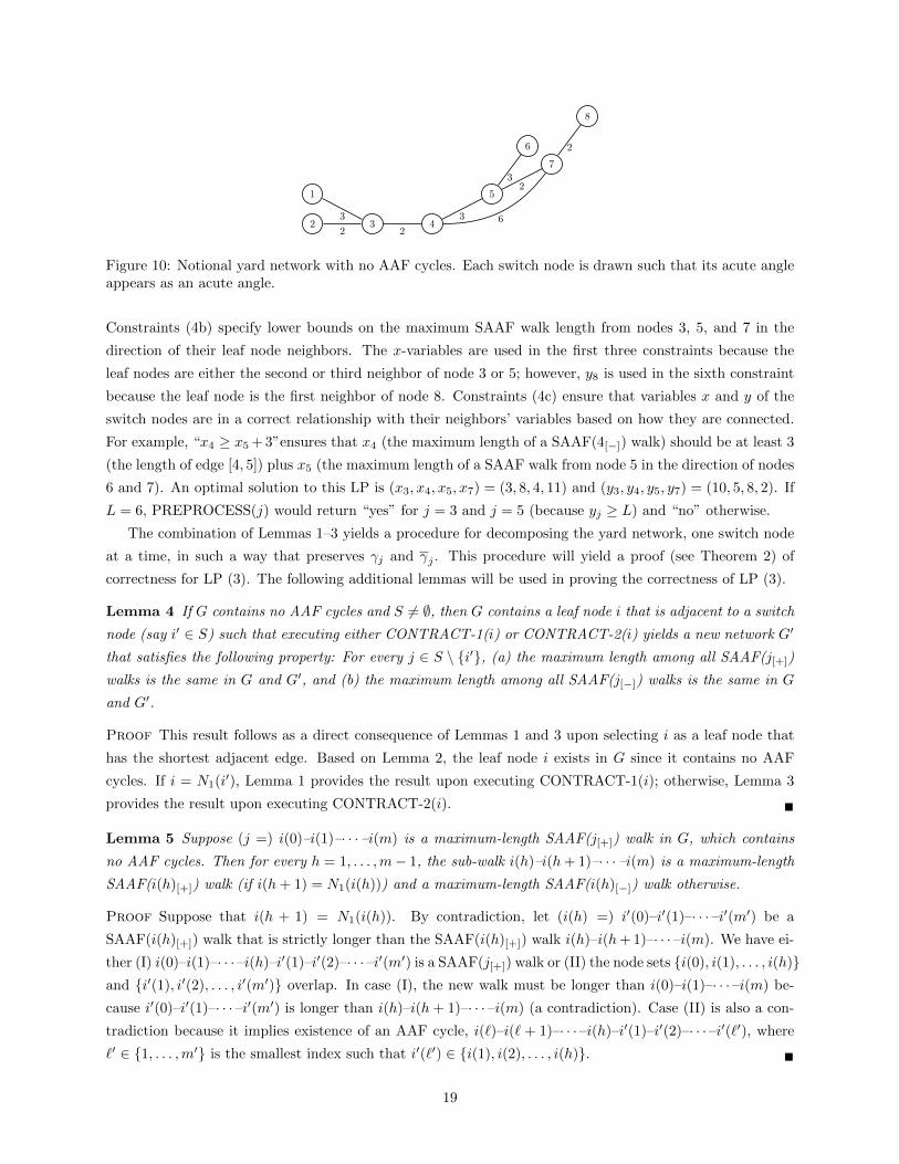
network depicted in Figure 10. (Note that 4–5–7–4 includes the acute angles at nodes 4 and 7; therefore,

the network has no AAF cycles.) The LP for this example is

min y3 + y4 + y5 + y7, (4a)

s.t. x3 ≥ 3, x3 ≥ 2, x5 ≥ 3, y7 ≥ 2; (4b)

y3 ≥ x4 + 2, x4 ≥ x5 + 3, x4 ≥ y7 + 6, y4 ≥ x3 + 2,

x5 ≥ y7 + 2, y5 ≥ y4 + 3, x7 ≥ y5 + 2, x7 ≥ y4 + 6. (4c)

18

2 3 4

5

7

8

6

1

2 2

33

23

6

2

Figure 10: Notional yard network with no AAF cycles. Each switch node is drawn such that its acute angleappears as an acute angle.

Constraints (4b) specify lower bounds on the maximum SAAF walk length from nodes 3, 5, and 7 in the

direction of their leaf node neighbors. The x-variables are used in the first three constraints because the

leaf nodes are either the second or third neighbor of node 3 or 5; however, y8 is used in the sixth constraint

because the leaf node is the first neighbor of node 8. Constraints (4c) ensure that variables x and y of the

switch nodes are in a correct relationship with their neighbors’ variables based on how they are connected.

For example, “x4 ≥ x5 + 3”ensures that x4 (the maximum length of a SAAF(4[−]) walk) should be at least 3

(the length of edge [4, 5]) plus x5 (the maximum length of a SAAF walk from node 5 in the direction of nodes

6 and 7). An optimal solution to this LP is (x3, x4, x5, x7) = (3, 8, 4, 11) and (y3, y4, y5, y7) = (10, 5, 8, 2). If

L = 6, PREPROCESS(j) would return “yes” for j = 3 and j = 5 (because yj ≥ L) and “no” otherwise.

The combination of Lemmas 1–3 yields a procedure for decomposing the yard network, one switch node

at a time, in such a way that preserves γj and γj . This procedure will yield a proof (see Theorem 2) of

correctness for LP (3). The following additional lemmas will be used in proving the correctness of LP (3).

Lemma 4 If G contains no AAF cycles and S 6= ∅, then G contains a leaf node i that is adjacent to a switch

node (say i′ ∈ S) such that executing either CONTRACT-1(i) or CONTRACT-2(i) yields a new network G′

that satisfies the following property: For every j ∈ S \ {i′}, (a) the maximum length among all SAAF(j[+])

walks is the same in G and G′, and (b) the maximum length among all SAAF(j[−]) walks is the same in G

and G′.

Proof This result follows as a direct consequence of Lemmas 1 and 3 upon selecting i as a leaf node that

has the shortest adjacent edge. Based on Lemma 2, the leaf node i exists in G since it contains no AAF

cycles. If i = N1(i′), Lemma 1 provides the result upon executing CONTRACT-1(i); otherwise, Lemma 3

provides the result upon executing CONTRACT-2(i). �

Lemma 5 Suppose (j =) i(0)–i(1)–· · · –i(m) is a maximum-length SAAF(j[+]) walk in G, which contains

no AAF cycles. Then for every h = 1, . . . ,m− 1, the sub-walk i(h)–i(h+ 1)–· · · –i(m) is a maximum-length

SAAF(i(h)[+]) walk (if i(h+ 1) = N1(i(h))) and a maximum-length SAAF(i(h)[−]) walk otherwise.

Proof Suppose that i(h + 1) = N1(i(h)). By contradiction, let (i(h) =) i′(0)–i′(1)–· · · –i′(m′) be a

SAAF(i(h)[+]) walk that is strictly longer than the SAAF(i(h)[+]) walk i(h)–i(h+ 1)–· · · –i(m). We have ei-

ther (I) i(0)–i(1)–· · · –i(h)–i′(1)–i′(2)–· · · –i′(m′) is a SAAF(j[+]) walk or (II) the node sets {i(0), i(1), . . . , i(h)}and {i′(1), i′(2), . . . , i′(m′)} overlap. In case (I), the new walk must be longer than i(0)–i(1)–· · · –i(m) be-

cause i′(0)–i′(1)–· · · –i′(m′) is longer than i(h)–i(h+ 1)–· · · –i(m) (a contradiction). Case (II) is also a con-

tradiction because it implies existence of an AAF cycle, i(`)–i(` + 1)–· · · –i(h)–i′(1)–i′(2)–· · · –i′(`′), where

`′ ∈ {1, . . . ,m′} is the smallest index such that i′(`′) ∈ {i(1), i(2), . . . , i(h)}. �

19

The following definitions will aid in proving the correctness of LP (3). For j ∈ S, define

Q(j) ≡ {i ∈ S : there exists a SAAF(i[+]) walk that includes j}, (5a)

Q(j) ≡ {i ∈ S : there exists a SAAF(i[−]) walk that includes j}. (5b)

Note that Q(j) ∩ Q(j) 6= ∅ implies existence of a closed AAF walk (by merging the SAAF(i[+]) and

SAAF(i[−]) walk), which therefore implies existence of an AAF cycle. We may therefore assume Q(j)∩Q(j) =

∅, ∀j ∈ S. Further, because j is reachable along a SAAF(i[+]) or SAAF(i[−]) walk if and only if i is reachable

along a SAAF(j[+]) or SAAF(j[−]) walk, Q(j)∪ Q(j) must equal the set of switch nodes reachable from node

j.

We now build towards a proof that an optimal solution of the LP (3) establishes the value of γi. Towards

this end, we first establish the impact of the subroutines CONTRACT-1(·) and CONTRACT-2(·) on LP (3).

Both CONTRACT-1(·) and CONTRACT-2(·) will remove a single switch node from the network. With

reference to the removed switch node i′, it will simplify exposition throughout the remainder of this section

to rename variables (xi, yi), i ∈ S \ {i′} as (w(i′)i , z

(i′)i ), i ∈ S \ {i′} as follows:

For i′ ∈ S, i ∈ Q(i′): w(i′)i ≡ yi and z

(i′)i ≡ xi, (6a)

For i′ ∈ S, i ∈ Q(i′): w(i′)i ≡ xi and z

(i′)i ≡ yi. (6b)

Lemma 6 Let i be a leaf node that is the first neighbor of a switch node i′, i.e., i = N1(i′). Let G denote

the original network, and let G′ denote the network after CONTRACT-1(i) has been executed. Similarly,

let LP(G) and LP(G′) denote the LP (3) under each network, and let Γ(G) and Γ(G′) denote the respective

sets of variables associated with these LPs. Then LP(G′) is a restriction of LP(G) in the sense that (a)

Γ(G′) ⊆ Γ(G) and (b) any feasible solution to LP(G′) can be extended into a feasible solution for LP(G) by

assigning values to the variables in Γ(G) \ Γ(G′).

Proof Let i′ denote the switch node that was removed by CONTRACT-1(i). The set of variables associated

with LP(G′) are (xj , yj), j ∈ S \ {i′}, while the set of variables associated with LP(G) are (xj , yj), j ∈ S.

This proves part (a) as Γ(G′) ∪ {xi′ , yi′} = Γ(G). Consider a solution (xj , yj), j ∈ S \ {i′} to LP (G′), and

according to Equations (6) let (w(i′)j , z

(i′)j ), j ∈ S \ {i′}, denote the corresponding values of (w

(i′)j , z

(i′)j ). We

now establish that this solution can be extended into a solution (xj , yj), j ∈ S, for LP (G) by assigning

yi′ = ce(i′,1) and xi′ = max{z(i′)N2(i′) + ce(i′,2), z

(i′)N3(i′) + ce(i′,3)}.

Assuming neither N2(i′) nor N3(i′) is a leaf node (with a description of the simplification in these special

cases to follow), the constraints in LP(G) but not LP(G′) are

yi′ ≥ ce(i′,1), (7a)

xi′ ≥ ce(i′,2) + z(i′)N2(i′), (7b)

w(i′)N2(i′) ≥ ce(i′,2) + yi′ , (7c)

xi′ ≥ ce(i′,3) + z(i′)N3(i′), (7d)

w(i′)N3(i′) ≥ ce(i′,3) + yi′ ; (7e)

it suffices to prove that each of these constraints is satisfied by (xj , yj), j ∈ S, along with the corresponding

20

values (w(i′)j , z

(i′)j ), j ∈ S \ {i′}. Constraint (7a) is satisfied at equality by yi′ = ce(i′,1). Constraints (7b)

and (7d) are satisfied because xi′ = max{z(i′)N2(i′) + ce(i′,2), z

(i′)N3(i′) + ce(i′,3)}. Feasibility to LP(G′) implies

w(i′)N2(i′) ≥ ce(i′,2) + ce(i′,1) and w

(i′)N3(i′) ≥ ce(i′,3) + ce(i′,1), respectively corresponding to the switch node N2(i′)

and N3(i′) in the direction of the new leaf nodes constructed by CONTRACT-1(i). Because yi′ = ce(i′,1),

Constraints (7c) and (7e) must therefore be satisfied. If N2(i′) is a leaf node, the proof is modified by

setting z(i′)N2(i′) = 0 and removing Constraint (7c); likewise, if N3(i′) is a leaf node, set z

(i′)N3(i′) = 0 and remove

Constraint (7e). Therefore, the solution (xj , yj), j ∈ S, satisfies all constraints that are included in LP(G)

but not not LP(G′) and must be feasible to LP(G). This completes the proof of part (b). �

Lemma 7 Let i be a leaf node with the smallest value of ce(i,1). (That is, i is a leaf node with the shortest-

length adjacent edge.) If i ∈ {N2(i′), N3(i′)} for some i′ ∈ S, then let G′ denote the network that results

upon executing CONTRACT-2(i). Let LP(G) and LP(G′) denote LP (3) under the original and contracted

network, and let Γ(G) and Γ(G′) denote their respective sets of variables. Then LP(G′) is a restriction of

LP(G) in the sense that (a) Γ(G′) ⊆ Γ(G) and (b) any feasible solution to LP(G′) can be extended into a

feasible solution for LP(G) by assigning values to the variables in Γ(G) \ Γ(G′).

Proof With the exception of node i′, all switch nodes from G remain switch nodes in G′; therefore,

Γ(G′) ∪ {xi′ , yi′} = Γ(G), proving part (a).

We now prove part (b). Towards this end, we assume without loss of generality that i = N3(i′) as the

proof for i = N2(i′) is symmetric. Let (xj , yj), j ∈ S \ {i′}, denote any feasible solution to LP(G′). In

accordance with Equations (6), let (w(i′)j , z

(i′)j ), j ∈ S \ {i′} denote the corresponding values of (w

(i′)j , z

(i′)j )

under solution (xj , yj), j ∈ S \ {i′}. Observe for k ∈ {1, 2} that z(i′)Nk(i′) = xNk(i′) and w

(i′)Nk(i′) = yNk(i′) if

N1(Nk(i′)) = i′; otherwise, z(i′)Nk(i′) = y

(i′)Nk(i′) and w

(i′)Nk(i′) = xNk(i′).

To prove part (b), it suffices to prove that (xi′ , yi′) can be assigned values (xi′ , yi′) such that the collection

(xj , yj), j ∈ S, satisfies the set of constraints

xi′ ≥ ce(i′,3), (8a)

yi′ ≥ z(i′)N1(i′) + ce(i′,1), (8b)

w(i′)N1(i′) ≥ xi′ + ce(i′,1), (8c)

xi′ ≥ z(i′)N2(i′) + ce(i′,2), (8d)

w(i′)N2(i′) ≥ yi′ + ce(i′,2), (8e)

that are included in LP(G) but not in LP(G′). (Note: Above we have assumed N1(i′) and N2(i′) are not leaf

nodes. We summarize at the end of this proof the modifications that are necessary if this is not the case.)

We claim that under the assignment xi′ = z(i′)N2(i′) + ce(i′,2) and yi′ = z

(i′)N1(i′) + ce(i′,1), the solution

(xj , yj), j ∈ S, satisfies System (8) and therefore proves the result. This assignment immediately satisfies

Constraints (8b) and (8d) at equality. Additionally, due to Constraints (3c), (3d), (3f), and (3g) of LP(G′)

corresponding to node i = N1(i′) in the direction of node N2(i′), we have that

w(i′)N1(i′) ≥ z

(i′)N2(i′) + ce(i′,1) + ce(i′,2), (9)

21

and corresponding to node i = N2(i′) in the direction of node N1(i′), we have that

w(i′)N2(i′) ≥ z

(i′)N1(i′) + ce(i′,1) + ce(i′,2). (10)

Therefore, upon substituting xi′ = z(i′)N2(i′)+ce(i′,2) into (9) and yi′ = z

(i′)N1(i′)+ce(i′,1) into (10), Constraints (8c)

and (8e) are satisfied.

To complete the proof, we now show that Constraint (8a) must be dominated by the remaining constraints

of LP(G) and therefore satisfied by (xj , yj), j ∈ S. To see this, let (i′ =) i(0)–i(1)–· · ·—i(m) (with edge

representation e(1)–e(2)–· · · –e(m)) denote any maximal SAAF(i′[−]) walk in G such that i(1) = N2(i′).

Then, LP(G) includes the constraint set

xi′ ≥ z(i′)i(1) + ce(1), (11a)

z(i′)i(h) ≥ z

(i′)i(h+1) + ce(h+1), ∀h = 1, . . . ,m− 2, (11b)

z(i′)i(m−1) ≥ ce(m), (11c)

where z(i′)i(m) does not appear on the right-hand side of Constraint (11c) because (via Lemma 2), maximal

SAAF(i′[+]) walks must end at a leaf node. Summing Constraints (11) yields xi′ ≥∑mh=1 ce(h) ≥ ce(m). By

assumption in this lemma’s statement, we selected i as a leaf node with the minimum-length adjacent edge,

and we must therefore have ce(m) ≥ ce(i′,3). Thus, we have that xi′ ≥ ce(i′,3) and Constraint (8a) is satisfied

by (xj , yj), j ∈ S.

Finally, we address the case where either N1(i′) or N2(i′) is a leaf node. If N1(i′) is a leaf node, the proof

proceeds exactly as above after assigning the value z(i′)N1(i′) = 0 and removing constraint (8c). Similarly, if

N2(i′) is a leaf node, apply the above proof after assigning zi′

N2(i′) = 0 and removing constraint (8e). �

Lemmas 6–7 lead to the following proof of correctness for LP (3).

Theorem 2 If G contains no AAF cycles, then (a) LP (3) is feasible and (b) yj = γj , ∀j ∈ S, in every

optimal solution.

Proof By iteratively selecting a leaf node i with the shortest adjacent edge, we can execute either CONTRACT-

1(i) or CONTRACT-2(i), depending on whether or not i is the first neighbor of some switch node. By

selecting i in this way, Lemma 4 guarantees the resulting network will preserve γj , j ∈ S, in each iteration,

with the exception that γi′ (where i′ is the neighbor of the leaf node i) is no longer defined. Because each

iteration removes a switch node, the number of iterations will be P ≡ |S|. Therefore, for p = 0, 1, . . . , P , let

Gp denote the network that results after p iterations and let LP(Gp) denote the corresponding instance of

LP (3). Define S(p) as the set of switch nodes in Gp such that

S = S(0) ⊇ S(1) ⊇ · · · ⊇ S(P ) = ∅. (12)

We complete the proof in two parts: We first establish the existence of a feasible solution for which yj = γj

for every switch node j ∈ S, thus establishing result (a); we then establish result (b) by proving that γj is a

lower bound on feasible yj , implying that yj = γj , ∀j ∈ S for any optimal solution under Objective (3a).

To prove result (a), we prove the following statement inductively: For all p = 0, 1, . . . , P , there exists

a feasible solution to LP(Gp) in which yj = γj and xj = γj , ∀j ∈ S(p). The base case, p = P , is trivial

22

because S(P ) = ∅; thus, LP(GP ) has no variables or constraints and is therefore vacuously feasible.

We now assume the result holds for a given value of p and prove the result must also hold for p − 1.

Let i′ denote the (unique) switch node in S(p− 1) \ S(p), let i denote the leaf node that was contracted to

remove node i′. Let (xj , yj), j ∈ S(p), denote a fixed solution that satisfies the induction hypothesis, i.e.,

yj = γj and xj = γj , ∀j ∈ S(p). Without loss of generality, we assume that i ∈ {N1(i′), N3(i′)} as the case

i = N2(i′) is symmetric to the case where i = N3(i′). By applying Lemma 6 (if i = N1(i′)) or Lemma 7 (if

i = N3(i′)), we may assign values to (xi′ , yi′) such that the collection {xj , yj : j ∈ S(p − 1)} is feasible to

LP(Gp−1). We now prove this assignment establishes case p− 1 in the inductive proof.

To prove yi′ = γi′ in case p − 1 (denoted “Result I”), let (i′ =) i(0)–i(1)–· · · –i(m) (with edges e(1)–

e(2)–· · · –e(m) such that e(1) = e(i′, 1)) denote a maximum-length SAAF(i′[+]) walk in Gp−1. Lemma 4

implies

γi′ =

m∑h=1

ce(h). (13)

We have either i(2) = N1(i(1)), which we denote as “(I, Case A),” or i(2) ∈ {N2(i(1)), N3(i(1))}, which we

denote as “(I, Case B)”. We prove that Lemmas 6–7 set yi′ = γi′ in each of these cases.

To prove (I, Case A), suppose i(2) = N1(i(1)). By Lemma 5, i(1)–i(2)–· · · –i(m) is a maximum-length

SAAF(i(1)[+]) walk. We proceed with the proof of this case by assuming that CONTRACT-2(i) was executed

in iteration p, and we end the proof of this case by summarizing the simplifications that result if CONTRACT-

1(i) was executed instead. Lemma 7 sets

yi′ = ce(i′,1) + z(i′)N1(i′), (14a)

= ce(1) + z(i′)i(1), (14b)

= ce(1) + yi(1), (14c)

= ce(1) + γi(1), (14d)

= ce(1) +

m∑h=2

ce(h), (14e)

which equals γi′ by Equation (13) and yields the result. In the above, Equation (14a) is taken directly

from Lemma 7. Equation (14b) holds because i(1) = N1(i′) in order for (i′ =) i(0)–i(1)–· · · –i(m) to be

a SAAF(i′[+]) walk. Equation (14c) employs the substitution z(i′)i(1) = yi(1) from Equation (6) because i′ is

reachable from i(1) along the SAAF(i(1)[−]) walk i(1)–i(0). Equation (14d) invokes the induction hypothesis,

and Equation (14e) utilizes the results that (Lemma 4) γi(1) equals the longest SAAF(i(1)[+]) walk length in

Gp−1 and (Lemma 5) the length of this walk is∑mh=2 ce(h). (If CONTRACT-1(i) was executed in iteration

p, then m = 1 and Equations (14) hold upon setting z(i′)N1(i′) = 0 as specified by Lemma 6).

In (I, Case B), Suppose i(2) ∈ {N2(i(1)), N3(i(1))}. By Lemma 5, i(1)–i(1)–· · · –i(m) is a maximum-

length SAAF(i(1)[−]) walk. In this case, the proof is analogous to case I with the modification that yi(1) is

replaced by xi(1) (because i′ is now reachable along the SAAF(i(1)[+]) walk i(1)–i(0)) and γi(1) is replaced

by γi(1) (upon invoking the induction hypothesis). The analog of Equation (14e) holds upon invoking

Lemmas 4–5 to guarantee that γi(1) =∑mh=2 ce(h). This completes the proof of (I, Case B) and Result I.

Towards proving that xi′ = γi′ in case p − 1 (denoted “Result II”), let (i′ =) i(0)–i(1)–· · · –i(m) (with

23

edge representation e(1)–e(2)–· · · –e(m)) denote a maximum-length SAAF(i′[−]) walk in Gp−1. We assume

without loss of generality that i(1) = N2(i′) (and therefore e(1) = e(i′, 2)) with reasoning to follow. If

i(1) = N3(i′), the earlier assumption that i ∈ {N1(i′), N3(i′)} permits the possibility that i = N3(i′)—and

i(1) is therefore the leaf node i, i.e., γi′ = ce(i′,3) = ce(i,1). If i 6= N3(i′), we have that i = N1(i′) and we can

assume i(1) = N2(i′) by swapping, if necessary, the second and third neighbors in the ordered adjacency list

of node i′. If i = N3(i′), the following rationale justifies assuming i(1) = N2(i′) without loss of generality:

By Lemma 2, any SAAF(i′[−]) walk whose first two nodes are i′ and N2(i′) can be extended into a maximal

SAAF(i′[−]) walk whose last edge is adjacent to a leaf node; if i(1) = N3(i′), our selecting i as a leaf node

with the shortest-length adjacent edge (having length ce(i,1) = ce(i′,3) = γi′) ensures that the last edge in

such a walk (and therefore the walk itself) is at least as long as γi′ and therefore also a maximum-length

SAAF(i′[−]) walk; we may therefore assume there is a maximum-length SAAF(i′[−]) walk among the set of

walks whose first two nodes are i′ and N2(i′). Lemma 4 now implies

γi′ =

m∑h=1

ce(h). (15)

Again, we have either (II, Case A) i(2) = N1(i(1)) or (II, Case B) i(2) ∈ {N2(i(1)), N3(i(1))}.In (II, Case A), suppose i(2) = N1(i(1)) such that Lemma 5 guarantees i(1)–i(2)–· · · –i(m) is a maximum-

length SAAF(i(1)[+]) walk. We will first prove this case assuming CONTRACT-1(i) was executed in iteration

p and then provide a summary of the simplifications that result if CONTRACT-2(i) was executed instead.

Lemma 6 sets xi′ = max{ce(i′,2) + z

(i′)N2(i′), ce(i′,3) + z

(i′)N3(i′)

}, which yields

xi′ = max{ce(i′,2) + z

(i′)N2(i′), ce(i′,3) + z

(i′)N3(i′)

}, (16a)

= max{ce(1) + yi(1), ce(i′,3) + z

(i′)N3(i′)

}, (16b)

= max{ce(1) + γi(1), ce(i′,3) + z

(i′)N3(i′)

}, (16c)

= max

{ce(1) +

m∑h=2

ce(h), ce(i′,3) + z(i′)N3(i′)

}, (16d)

= max{γi′ , ce(i′,3) + z

(i′)N3(i′)

}, (16e)

after applying the logic of Equations (14) to the first term in the maximum. We now prove that γi′ ≥ce(i′,3) + z

(i′)N3(i′) (and therefore xi′ = γi′). By Lemma 5 and the induction hypothesis, z

(i′)N3(i′) equals either

γN3(i′) (if N1(N3(i′)) = i′) or γN3(i′) (otherwise); therefore, there exists a SAAF walk W of length zN3(i′)

that begins at node N3(i′). One of these cases yields that W is a SAAF(N3(i′)[−]) walk and N3(i′)–i′

is a SAAF(N3(i′)[+]) walk while the other yields that W is a SAAF(N3(i′)[+]) walk and N3(i′)–i′ is a

SAAF(N3(i′)[−]) walk; thus, W cannot include i′ (as this would imply Q(i′)∩ Q(i′) 6= ∅ and the existence of

an AAF cycle in Gp−1). Therefore, we can create a SAAF(i′[−]) walk by merging [i′, N3(i′)] = e(i′, 3) with

the edges of W . This walk has length ce(i′,3) + z(i′)N3(i′), and we must therefore have γi′ ≥ ce(i′,3) + z

(i′)N3(i′)

because γi′ is defined as the maximum length among SAAF(i′[−]) walks. This proves that xi′ = γi′ if

CONTRACT-1(i) is executed in iteration p. If CONTRACT-2(i) is executed instead, then Lemma 7 sets

xi′ = ce(i′,2) + z(i′)N2(i), which equals γi′ due to logic analagous to Equations (16a)–(16e).

In (II, Case B), suppose i(2) ∈ {N2(i(1)), N3(i(1))}. The proof of this case is identical to case (II:A)

24

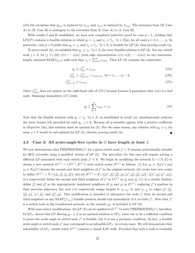
with the exception that yi(1) is replaced by xi(1) and γi(1) is replaced by γi(1). The extension from (II, Case

A) to (II, Case B) is analogous to the extension from (I, Case A) to (I, Case B).

With results I and II established, we have now completed inductive proof for case p − 1, yielding that

LP(Gp) contains a feasible solution in which yj = γj and xj = γj , ∀j ∈ S(p), for all cases p = 0, 1, . . . , p. In

particular, case p = 0 yields that yj = γj and xj = γj , ∀j ∈ S, is feasible for LP (3), thus proving result (a).

To prove result (b), we establish that yj ≥ γj , ∀j ∈ S, for every feasible solution to LP (3). For any switch

node j ∈ S, let (j =) i(0)–i(1)–· · · –i(m) (with edge representation e(1)–e(2)–· · · –e(m)) be any maximum-

length, maximal SAAF(j[+]) walk such that γj =∑mh=1 ce(h). Then LP (3) contains the constraints

yj ≥ z(j)i(1) + ce(1), (17a)

z(j)i(h) ≥ z

(j)i(h+1) + ce(h+1), ∀h = 1, . . . ,m− 2, (17b)

z(j)i(m−1) ≥ ce(m), (17c)

where z(j)i(m) does not appear on the right-hand side of (17c) because Lemma 2 guarantees that i(m) is a leaf

node. Summing inequalities (17) yields

yj ≥m∑h=1

ce(h) = γj . (18)

Note that the feasible solution with yj = γj , ∀j ∈ S, as established in result (a), simultaneously achieves

the lower bound (18) provided for each yj , j ∈ S. Because all y-variables appear with a positive coefficient

in Objective (3a), this solution must be optimal for (3). For the same reason, any solution with yj > γj for

some j ∈ S would be sub-optimal for LP (3), thereby proving result (b). �

4.3 Case 2: All acute-angle-free cycles in G have length at least L

We now demonstrate that PREPROCESS(j?) for a given switch node j? ∈ S remains polynomially solvable

for BCL networks using a modified version of LP (3). The procedure for this case will require solving a

different LP associated with each switch node j? ∈ S. We begin by modifying the network G = (N,E) to

obtain a new network G(j?) = (N (j?), E(j?)) with switch nodes S(j?) as follows: (i) Let j2 ≡ N2(j?) and

j3 ≡ N3(j?) denote the second and third neighbors of j? in the original network; (ii) create four new nodes

to define N (j?) = N ∪ {j′2, j′′2 , j′3, j′′3 }; (iii) set E(j?) = E ∪ {[j?, j′2], [j′′2 , j2], [j?, j′3], [j′′3 , j3]} \ {[j?, j2], [j?, j3]};(iv) respectively define the second and third neighbors of j? in G(j?) as j′2 and j′3; (v) in a similar fashion,

define j′′2 and j′′3 as the appropriately numbered neighbors of j2 and j3 in G(j?), replacing j?’s position in

their previous adjacency list; and (vi) respectively assign lengths 0, cj?,j2 , 0, and cj?,j3 to edges [j?, j′2],

[j′′2 , j2], [j?, j′3], and [j′′3 , j3]. This modification is intended to disconnect the node j? from its second and

third neighbors as any SAAF(j?[+]) feasible position should end immediately if it re-visits j?. Note that j?

is a switch node in the transformed network, so the variable yj? is included in LP (3).

With some minor modifications, the LP (3) can be applied to G(j?) to solve PREPROCESS(j?); hereafter,

let LPj? denote this LP. Having yj? ≥ L in an optimal solution to LPj? turns out to be a sufficient condition

to prove the acute angle at switch node j? is feasible, but it is not a necessary condition. In fact, a feasible

acute angle at switch node j? may correspond to an infeasible LPj? in certain cases. We will demonstrate that

infeasibility of LPj? results when G(j?) contains a closed AAF walk. Provided that such a walk is reachable

25

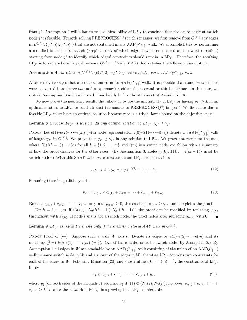
from j?, Assumption 2 will allow us to use infeasibility of LPj? to conclude that the acute angle at switch

node j? is feasible. Towards solving PREPROCESS(j?) in this manner, we first remove from G(j?) any edges

in E(j?) \{[j?, j′2], [j?, j′3]} that are not contained in any AAF(j?[+]) walk. We accomplish this by performing

a modified breadth first search (keeping track of which edges have been reached and in what direction)

starting from node j? to identify which edges’ constraints should remain in LPj? . Therefore, the resulting

LPj? is formulated over a yard network G(j?) = (N (j?), E(j?)) that satisfies the following assumption.

Assumption 4 All edges in E(j?) \ {e(j?, 2), e(j?, 3)} are reachable via an AAF(j?[+]) walk.

After removing edges that are not contained in an AAF(j?[+]) walk, it is possible that some switch nodes

were converted into degree-two nodes by removing either their second or third neighbor—in this case, we

restore Assumption 3 as summarized immediately before the statement of Assumption 3.

We now prove the necessary results that allow us to use the infeasibility of LPj? or having yj? ≥ L in an

optimal solution to LPj? to conclude that the answer to PREPROCESS(j?) is “yes.” We first note that a

feasible LPj? must have an optimal solution because zero is a trivial lower bound on the objective value.

Lemma 8 Suppose LPj? is feasible. In any optimal solution to LPj? , yj? ≥ γj? .

Proof Let e(1)–e(2)–· · · –e(m) (with node representation i(0)–i(1)–· · · –i(m)) denote a SAAF(j?[+]) walk

of length γj? in G(j?). We prove that yj? ≥ γj? in any solution to LPj? . We prove the result for the case

where N1(i(h − 1)) = i(h) for all h ∈ {1, 2, . . . ,m} and i(m) is a switch node and follow with a summary

of how the proof changes for the other cases. (By Assumption 3, nodes {i(0), i(1), . . . , i(m − 1)} must be

switch nodes.) With this SAAF walk, we can extract from LPj? the constraints

yi(h−1) ≥ ce(h) + yi(h), ∀h = 1, . . . ,m. (19)

Summing these inequalities yields

yj? = yi(0) ≥ ce(1) + ce(2) + · · ·+ ce(m) + yi(m). (20)

Because ce(1) + ce(2) + · · ·+ ce(m) = γi and yi(m) ≥ 0, this establishes yj? ≥ γj? and completes the proof.

For h = 1, . . . ,m, if i(h) ∈ {N2(i(h − 1)), N3(i(h − 1))} the proof can be modified by replacing yi(h)

throughout with xi(h). If node i(m) is not a switch node, the proof holds after replacing yi(m) with 0. �

Lemma 9 LPj? is infeasible if and only if there exists a closed AAF walk in G(j?).

Proof Proof of (←): Suppose such a walk W exists. Denote its edges by e(1)–e(2)–· · · –e(m) and its

nodes by (j =) i(0)–i(1)–· · · –i(m) (= j). (All of these nodes must be switch nodes by Assmption 3.) By

Assumption 4 all edges in W are reachable by an AAF(j?[+]) walk consisting of the union of an AAF(j?[+])

walk to some switch node in W and a subset of the edges in W ; therefore LPj? contains two constraints for

each of the edges in W . Following Equation (20) and substituting i(0) = i(m) = j, the constraints of LPj?

imply

yj ≥ ce(1) + ce(2) + · · ·+ ce(m) + yj , (21)

where yj (on both sides of the inequality) becomes xj if i(1) ∈ {N2(j), N3(j)}; however, ce(1) + ce(2) + · · ·+ce(m) ≥ L because the network is BCL, thus proving that LPj? is infeasible.

26

Proof of (→): We now prove that LPj? must be feasible if no such closed AAF walk exists. Towards

this end, observe that each switch node i ∈ S(j?) yields exactly one constraint from Constraints (3b)–(3d):

Define vi,N1(i) as the dual variable associated with this constraint. Similarly, each switch node i ∈ S(j?)

yields exactly one constraint for each k ∈ {2, 3} from Constraints (3e)–(3g): Let vi,Nk(i), k ∈ {2, 3}, denote

the associated dual variable. For simplicity of exposition, let vi,j ≡ 0 whenever [i, j] ∈ E(j?) but node i is

a leaf node (i.e., |N(i)| = 1). By Farkas’ lemma, LPj? is infeasible if and only if there is a solution to the

system

∑i∈S(j?)

3∑k=1

ce(i,k)vi,Nk(i) > 0, (22a)

− vN1(i),i + vi,N2(i) + vi,N3(i) = 0, ∀i ∈ S(j?), (22b)

vi,N1(i) − vN2(i),i − vN3(i),i = 0, ∀i ∈ S(j?), (22c)

vi,Nk(i) ≥ 0, ∀i ∈ S(j?), (22d)

vNk(i),i ≥ 0, ∀i ∈ S(j?). (22e)

Constraints (22b)–(22e) comprise a “feasible circulation” polyhedron (e.g., as defined in [3]) on a directed

network G(j?) = (N (j?), A(j?)) in which each node i ∈ N (j?) has been split into two nodes (i〈1〉 and i〈2〉)

such that Constraint (22b) defines the flow balance constraint for node i〈1〉 and Constraint (22c) defines

the flow balance constraint for node i〈2〉. Let N (j?) = {i〈β〉 : i ∈ N (j?), β ∈ {1, 2}} denote the expanded

set of nodes. Upon interpreting Constraints (22b) and (22c) as flow balance constraints for nodes i〈1〉 and

i〈2〉, i ∈ N (j?), vi,j can be interpreted as the flow on a directed arc from either node i〈1〉 ∈ N (j?) or node

i〈2〉 ∈ N (j?) to either node j〈1〉 ∈ N (j?) or node j〈2〉 ∈ N (j?). For [i, j] ∈ E(j?), let

b(i, j) =

{1 if j = N1(i),

2 otherwise,and b(j, i) =

{1 if i = N1(j),

2 otherwise,(23)

The directed arcs in the resulting network are

A(j?) =⋃

[i,j]∈E(j?)

{(i〈3−b(i,j)〉, j〈b(j,i)〉), (j〈3−b(j,i)〉, i〈b(i,j)〉)

}. (24)

(Note: Figure 11 depicts the resulting directed network G(j?) for the yard network in Figure 2 assuming

j? = 14. Although unnecessary for the purposes of this proof, it is interesting to note that the directed walks

of G(j?) beginning at node j?〈2〉 correspond to SAAF(j?[+]) walks of G(j?).)

Now suppose LPj? is infeasible. Then, by Farkas’ lemma, there exists a solution v to System (22). By

Constraint (22a), we must have that v 6= 0. By the flow decomposition theorem (see, e.g., [3, pp. 80–81]),

v (and indeed any solution to Equations (22b)–(22e)) may be represented as a summation of flows around

directed cycles, of which there must be at least one because v 6= 0. Let W be any directed cycle in G(j?),

and denote the nodes of W as i(0)〈β(0)〉–i(1)〈β(1)〉–· · · –i(m)〈β(m)〉 (= i(0)〈β(0)〉), where i(h) ∈ S(j?) and

β(h) ∈ {1, 2}, ∀h ∈ {1, . . . ,m}. In order for this to be a directed walk, we must have

{(i(h− 1)〈β(h−1)〉, i(h)〈β(h)〉), (i(h)〈β(h)〉, i(h− 1)〈β(h−1)〉)} ⊆ A(j?), ∀h ∈ {1, . . . ,m}, (25)

27

12

34

56

78

9

10

11

13

14

12

15

16

17

18

19

20

21

22

23

24

25

26

29

28

27

30

31

32

36

35

34

33

37

38

41

42

40

39

44

43

β=

1β=

2β=

1β=

2β=

1β=

2β=

1β=

2

Fig

ure

11:

Dir

ecte

dn

etw

ork

exp

ansi

onG

(j?)

=(N

(j?),A

(j?))

for

the

yard

net

workG

inF

igu

re2

wh

enj?

=14.

For

each

nod

ei〈β〉 ,

the

valu

esofi

andβ

are

lab

eled

usi

ng

the

fain

tre

dli

nes

that

inte

rsec

tth

en

od

e.D

ott

edre

darc

s(

)d

enote

arc

sth

at

wer

en

ot

incl

ud

edinG

(14)

bec

au

seth

eco

rres

pon

din

ged

gew

asn

otre

ach

able

by

anA

AF

(14 [

+])

walk

inG

(14).

Th

ick

blu

earc

s(

)in

dic

ate

ad

irec

ted

walk

that

beg

ins

at

nod

e14〈2〉

in

G(1

4)—

such

aw

alk

mu

stal

way

sco

rres

pon

dto

an

AA

F(1

4 [+

])w

alk

inG

.

28

and therefore (due to Equation (24) for [i, j] = [i(h− 1), i(h)] and [i, j] = [i(h), i(h+ 1)])

β(h) = b(i(h), i(h− 1)) = 3− b(i(h), i(h+ 1)), ∀h = 1, . . . ,m, (26)

where β(m + 1) ≡ β(1) and i(m + 1) ≡ i(1). In addition, each [i, j] ∈ E(j?) yields exactly one directed arc

from i〈1〉 or i〈2〉 in N (j?) to either j〈1〉 or j〈2〉 in N (j?); therefore, due to Assumption 1, the directed cycle

W must satisfy

i(h− 1) 6= i(h+ 1), ∀h = 1, . . . ,m. (27)

We now demonstrate for h = 1, . . . ,m, the edge pair {[i(h− 1), i(h)], [i(h), i(h + 1)]} is not an acute angle.

Towards this end, suppose i(h − 1) 6= N1(i(h)). Then b(i(h), i(h − 1)) = 2 according to Equation (23);

however, Equation (26) now implies that b(i(h), i(h + 1)) = 1, which implies under Equation (23) that

i(h + 1) = N1(i(h)). Therefore, either i(h − 1) or i(h + 1) is the first neighbor of i(h), proving that

{[i(h− 1), i(h)], [i(h), i(h+ 1)]} is not an acute angle. The sequence of nodes i(0)–i(1)–· · · –i(m) (= i(0)) is

therefore a closed AAF walk in G(j?). This completes the proof. �

Lemma 10 Suppose LPj? is feasible. In any optimal solution to LPj? , yj? > γj? only if there exists a switch

node j and an AAF cycle W with nodes (j =) i(0)–i(1)–· · · –i(m) (= j) such that (a) {[i(m− 1), j], [j, i(1)]}is an acute angle and (b) j is reachable via an AAF(j?[+]) walk that intersects W only at the switch node j

(and whose last two nodes are therefore N1(j) and j).

Proof Suppose yj? > γj? in an optimal solution to LPj? . By Theorem 2, the network cannot be devoid

of AAF cycles or else yj? = γj? in every optimal solution. Therefore, the network contains an AAF cycle

W with nodes i(0)–i(1)–· · · –i(m), and all of the edges in W must be reachable via an AAF(j?[+]) walk due

to Assumption 4. Let j = i(0) = i(m), which must be a switch node by Assumption 3. Due to Lemma 9,

{[i(m− 1), j], [j, i(1)]} must be an acute angle, or else LPj? would be infeasible.

By contradiction, suppose every AAF(j?[+]) walk that ends at switch node j includes some edge in W .

For the remainder of this proof, the phrase “traverses edge (i′, j′)” conveys that i′ appears immediately

before j′ on an AAF(j?[+], j) walk.

Let h′ ∈ {1, . . . ,m−1} denote the largest value for which there exists an AAF(j?[+], j) walk that traverses

(i(h′), i(h′ − 1)). (If no such value of h′ exists, the result is proved by contradiction because edge [j, i(1)]

must be unreachable.) Similarly, let h′′ ∈ {1, . . . ,m} denote the smallest value for which there exists an

AAF(j?[+], j) walk that traverses (i(h′′), i(h′′ + 1)). (Similarly, the value of h′′ must be defined or else

[i(m − 1), j] is unreachable.) By definition of h′, we have the following results: No AAF(j?[+], j) walk

traverses both (i(h′), i(h′ − 1)) and (i(h′ + 1), i(h′)). And by definition of h′′ we have the following: No

AAF(j?[+], j) walk traverses both (i(h′′), i(h′′ + 1)) and (i(h′′ − 1), i(h′′)). We now prove result (b) in three

cases: (I) h′ = h′′, (II) h′ < h′′, and (III) h′ > h′′.

Proof of (Case I): Let h = h′ = h′′ and consider two AAF(j?[+], j) walks: W ′, which traverses (i(h), i(h−1)) but not (i(h+ 1), i(h)); and W ′′, which traverses (i(h), i(h+ 1)) but not (i(h− 1), i(h)). By Property 1,

both of these walks must arrive to node i(h) from a common neighbor, i′ ∈ N (j?). We have identified the

three edges {[i′, i(h)], [i(h), i(h− 1)], [i(h), i(h+ 1)]} as adjacent to node i(h); however, no pair of edges from

this subset can be an acute angle. The pairs {[i′, i(h)], [i(h), i(h− 1)]} and {[i′, i(h)], [i(h), i(h+ 1)]} cannot

29

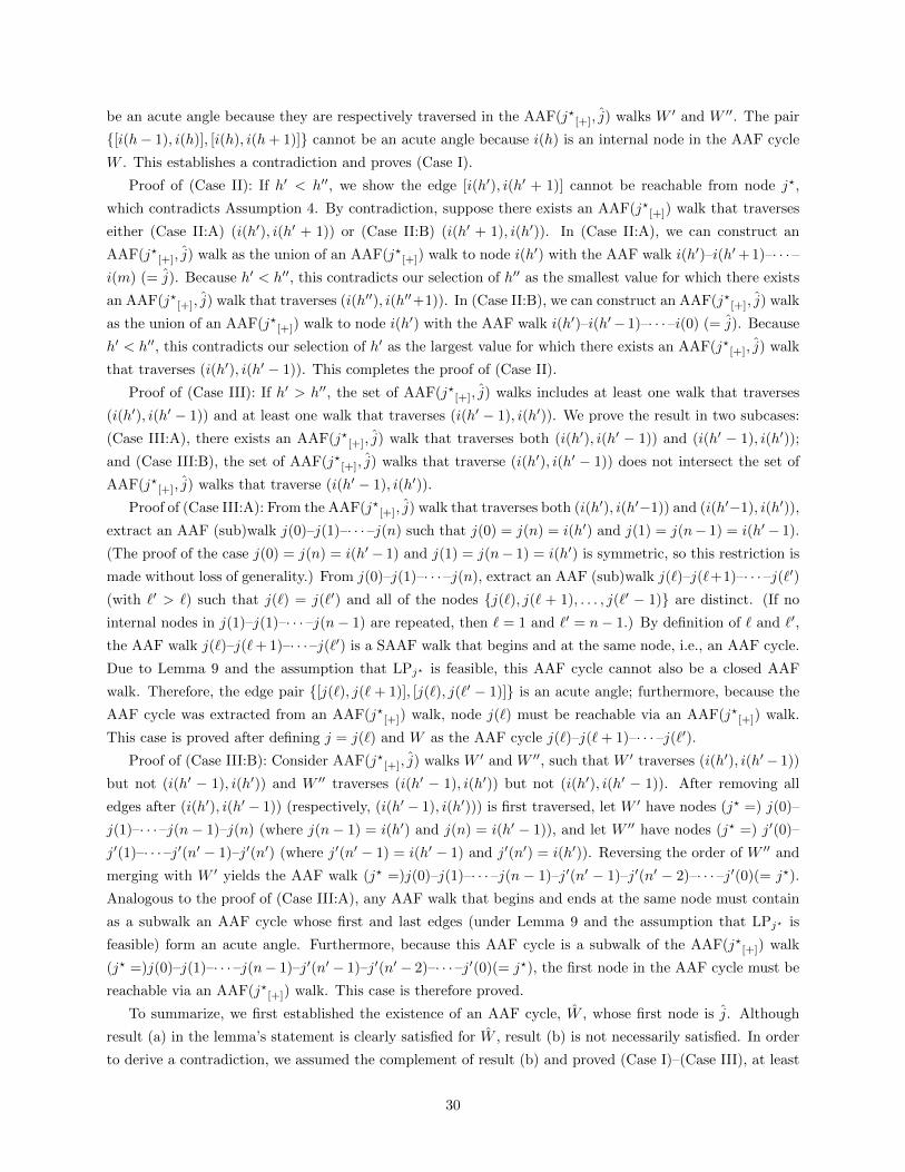
be an acute angle because they are respectively traversed in the AAF(j?[+], j) walks W ′ and W ′′. The pair

{[i(h− 1), i(h)], [i(h), i(h+ 1)]} cannot be an acute angle because i(h) is an internal node in the AAF cycle

W . This establishes a contradiction and proves (Case I).

Proof of (Case II): If h′ < h′′, we show the edge [i(h′), i(h′ + 1)] cannot be reachable from node j?,

which contradicts Assumption 4. By contradiction, suppose there exists an AAF(j?[+]) walk that traverses

either (Case II:A) (i(h′), i(h′ + 1)) or (Case II:B) (i(h′ + 1), i(h′)). In (Case II:A), we can construct an

AAF(j?[+], j) walk as the union of an AAF(j?[+]) walk to node i(h′) with the AAF walk i(h′)–i(h′+ 1)–· · · –i(m) (= j). Because h′ < h′′, this contradicts our selection of h′′ as the smallest value for which there exists

an AAF(j?[+], j) walk that traverses (i(h′′), i(h′′+1)). In (Case II:B), we can construct an AAF(j?[+], j) walk

as the union of an AAF(j?[+]) walk to node i(h′) with the AAF walk i(h′)–i(h′− 1)–· · · –i(0) (= j). Because

h′ < h′′, this contradicts our selection of h′ as the largest value for which there exists an AAF(j?[+], j) walk

that traverses (i(h′), i(h′ − 1)). This completes the proof of (Case II).

Proof of (Case III): If h′ > h′′, the set of AAF(j?[+], j) walks includes at least one walk that traverses

(i(h′), i(h′ − 1)) and at least one walk that traverses (i(h′ − 1), i(h′)). We prove the result in two subcases:

(Case III:A), there exists an AAF(j?[+], j) walk that traverses both (i(h′), i(h′ − 1)) and (i(h′ − 1), i(h′));

and (Case III:B), the set of AAF(j?[+], j) walks that traverse (i(h′), i(h′ − 1)) does not intersect the set of

AAF(j?[+], j) walks that traverse (i(h′ − 1), i(h′)).

Proof of (Case III:A): From the AAF(j?[+], j) walk that traverses both (i(h′), i(h′−1)) and (i(h′−1), i(h′)),

extract an AAF (sub)walk j(0)–j(1)–· · · –j(n) such that j(0) = j(n) = i(h′) and j(1) = j(n− 1) = i(h′− 1).

(The proof of the case j(0) = j(n) = i(h′ − 1) and j(1) = j(n− 1) = i(h′) is symmetric, so this restriction is

made without loss of generality.) From j(0)–j(1)–· · · –j(n), extract an AAF (sub)walk j(`)–j(`+1)–· · · –j(`′)(with `′ > `) such that j(`) = j(`′) and all of the nodes {j(`), j(` + 1), . . . , j(`′ − 1)} are distinct. (If no

internal nodes in j(1)–j(1)–· · · –j(n− 1) are repeated, then ` = 1 and `′ = n− 1.) By definition of ` and `′,

the AAF walk j(`)–j(`+ 1)–· · · –j(`′) is a SAAF walk that begins and at the same node, i.e., an AAF cycle.

Due to Lemma 9 and the assumption that LPj? is feasible, this AAF cycle cannot also be a closed AAF

walk. Therefore, the edge pair {[j(`), j(` + 1)], [j(`), j(`′ − 1)]} is an acute angle; furthermore, because the

AAF cycle was extracted from an AAF(j?[+]) walk, node j(`) must be reachable via an AAF(j?[+]) walk.

This case is proved after defining j = j(`) and W as the AAF cycle j(`)–j(`+ 1)–· · · –j(`′).Proof of (Case III:B): Consider AAF(j?[+], j) walks W ′ and W ′′, such that W ′ traverses (i(h′), i(h′− 1))

but not (i(h′ − 1), i(h′)) and W ′′ traverses (i(h′ − 1), i(h′)) but not (i(h′), i(h′ − 1)). After removing all

edges after (i(h′), i(h′ − 1)) (respectively, (i(h′ − 1), i(h′))) is first traversed, let W ′ have nodes (j? =) j(0)–

j(1)–· · · –j(n− 1)–j(n) (where j(n− 1) = i(h′) and j(n) = i(h′ − 1)), and let W ′′ have nodes (j? =) j′(0)–

j′(1)–· · · –j′(n′ − 1)–j′(n′) (where j′(n′ − 1) = i(h′ − 1) and j′(n′) = i(h′)). Reversing the order of W ′′ and

merging with W ′ yields the AAF walk (j? =)j(0)–j(1)–· · · –j(n − 1)–j′(n′ − 1)–j′(n′ − 2)–· · · –j′(0)(= j?).

Analogous to the proof of (Case III:A), any AAF walk that begins and ends at the same node must contain

as a subwalk an AAF cycle whose first and last edges (under Lemma 9 and the assumption that LPj? is

feasible) form an acute angle. Furthermore, because this AAF cycle is a subwalk of the AAF(j?[+]) walk

(j? =)j(0)–j(1)–· · · –j(n− 1)–j′(n′ − 1)–j′(n′ − 2)–· · · –j′(0)(= j?), the first node in the AAF cycle must be

reachable via an AAF(j?[+]) walk. This case is therefore proved.

To summarize, we first established the existence of an AAF cycle, W , whose first node is j. Although

result (a) in the lemma’s statement is clearly satisfied for W , result (b) is not necessarily satisfied. In order

to derive a contradiction, we assumed the complement of result (b) and proved (Case I)–(Case III), at least

30

one of which describes the set of AAF(j?[+], j) walks. In (Case I)–(Case II), we arrived at the contradiction

in order to prove that results (a) and (b) must both be satisfied for W and j. In (Case III), results (a) and

(b) are not satisfied for W and j, but we establish the existence of another AAF cycle W and node j for

which (a) and (b) are both satisfied. This completes the proof.

Theorem 3 For BCL networks, the acute angle at switch node j? ∈ S(j?) is feasible if and only if (a) LPj?

is infeasible or (b) yj? ≥ L in an optimal solution of LPj? .

Proof Proof of (→): Suppose the acute angle at switch node j? is feasible, i.e., γj? ≥ L. If LPj? is feasible,

Lemma 8 establishes that yj? ≥ γj? (≥ L). This completes the proof of (→).

Proof of (←, Case I): Suppose LPj? is infeasible. By Lemma 9, there exists a closed AAF walk W

in G(j?). By Assumption 4, all of the edges in W must be reachable via an AAF(j?[+]) walk. Therefore

(reaching one such edge and then traversing all of the edges of W in sequence), there exists an AAF(j?[+])

walk (j? =) i(0)–i(1)–· · · –i(m) such that W is defined by the nodes i(n)–i(n+ 1)–· · · –i(m) for some n < m.

Within this walk, let ` denote the smallest value in {1, . . . ,m} such that i(`) ∈ {i(0), i(1), . . . , i(` − 1)},where ` ≤ m because i(n) = i(m). By our selection of `, the walk (j? =) i(0)–i(1)–· · · –i(`) is a SAAF(j?[+])

walk; moreover, because the walk visits i(`) twice, Assumption 2 implies its length must be at least L. The

acute angle at switch node j? ∈ N (j?) is therefore feasible.

Proof of (←, Case II): Suppose LPj? is feasible and yj? ≥ L in an optimal solution of LPj? . We prove

the result in two subcases: (←, Case II:A) yj? = γj? in an optimal solution of LPj? or (←, Case II:B)

yj? > γj? in an optimal solution of LPj? . In (←, Case II:A), the result is immediate due to Lemma 8

because (γj? =) yj? ≥ L. In (←, Case II:B), Lemma 10 implies the existence of an AAF cycle W with

nodes (j =) i(0)–i(1)–· · · –i(m) (= j) such that (a) {[i(m − 1), j], [j, i(1)]} is an acute angle and (b) j is

reachable via an AAF(j?[+]) walk that intersects W only at j. If all of the nodes in the AAF(j?[+]) walk are

unique, the union of this AAF(j?[+]) walk with W therefore yields a SAAF(j?[+]) walk in which only node

j is repeated; if some node in the AAF(j?[+]) walk is repeated, consider instead its subwalk leading up to

the first repeated node. By Assumption 2, this walk must have length at least L. Therefore, the acute angle

at switch node j? ∈ N (j?) is feasible. �

Theorem 4 PREPROCESS(j?) is polynomially solvable for BCL networks.

Proof By Theorem 3, PREPROCESS(j?) can be solved using LPj? , whose formulation is polynomial in

the size of the PREPROCESS(j?) input. The result follows because LPs are polynomially solvable [11]. �

We conclude this section by formalizing procedures to (in Remark 1) ensure Assumption 4 is satisfied and

(in Remark 2) check whether a yard network is BCL.

Remark 1 Suppose G(j?) = (N (j?), E(j?)) has been created without removing edges that are not reachable

via an AAF(j?[+]) walk. From G(j?), we can apply the transformation described in the proof of Lemma 9

to obtain the directed network G(j?) = (N (j?), A(j?)). As demonstrated in the Lemma 9 proof, directed

walks in G(j?) correspond to (possibly non-simple) AAF walks in G(j?). Therefore, we may identify edges

[i, j] ∈ E(j?) that are unreachable by performing a traditional breadth first search (see, e.g., [3, p.76]) over

G(j?), beginning at node j?〈2〉 ∈ N (j?), in order to identify the subset of directed arcs A ⊆ A(j?) that exist in

at least one directed walk that begins at node j?〈2〉. We then remove each edge [i, j] from E(j?) if A contains

no arcs with one endpoint in each of the node subsets {i〈1〉, i〈2〉} ⊆ N (j?) and {j〈1〉, j〈2〉} ⊆ N (j?). �

31

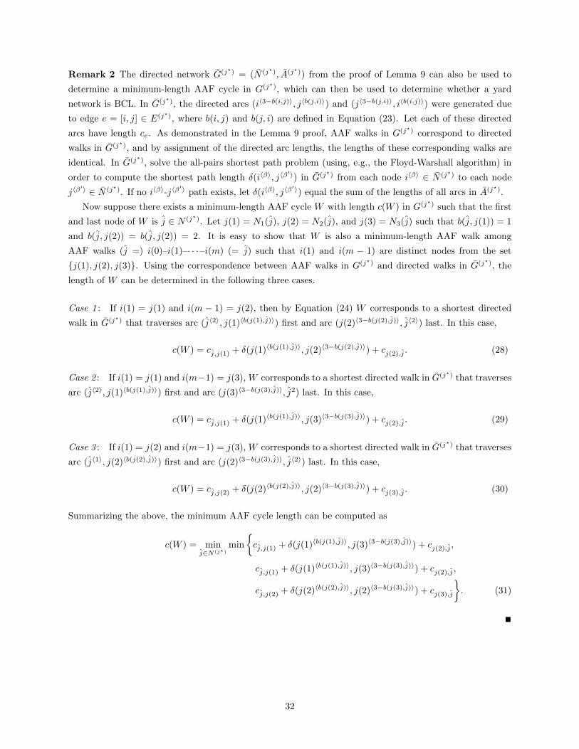
Remark 2 The directed network G(j?) = (N (j?), A(j?)) from the proof of Lemma 9 can also be used to

determine a minimum-length AAF cycle in G(j?), which can then be used to determine whether a yard

network is BCL. In G(j?), the directed arcs (i〈3−b(i,j)〉, j〈b(j,i)〉) and (j〈3−b(j,i)〉, i〈b(i,j)〉) were generated due

to edge e = [i, j] ∈ E(j?), where b(i, j) and b(j, i) are defined in Equation (23). Let each of these directed

arcs have length ce. As demonstrated in the Lemma 9 proof, AAF walks in G(j?) correspond to directed

walks in G(j?), and by assignment of the directed arc lengths, the lengths of these corresponding walks are

identical. In G(j?), solve the all-pairs shortest path problem (using, e.g., the Floyd-Warshall algorithm) in

order to compute the shortest path length δ(i〈β〉, j〈β′〉) in G(j?) from each node i〈β〉 ∈ N (j?) to each node

j〈β′〉 ∈ N (j?). If no i〈β〉-j〈β

′〉 path exists, let δ(i〈β〉, j〈β′〉) equal the sum of the lengths of all arcs in A(j?).

Now suppose there exists a minimum-length AAF cycle W with length c(W ) in G(j?) such that the first

and last node of W is j ∈ N (j?). Let j(1) = N1(j), j(2) = N2(j), and j(3) = N3(j) such that b(j, j(1)) = 1

and b(j, j(2)) = b(j, j(2)) = 2. It is easy to show that W is also a minimum-length AAF walk among

AAF walks (j =) i(0)–i(1)–· · · –i(m) (= j) such that i(1) and i(m − 1) are distinct nodes from the set

{j(1), j(2), j(3)}. Using the correspondence between AAF walks in G(j?) and directed walks in G(j?), the

length of W can be determined in the following three cases.

Case 1 : If i(1) = j(1) and i(m − 1) = j(2), then by Equation (24) W corresponds to a shortest directed

walk in G(j?) that traverses arc (j〈2〉, j(1)〈b(j(1),j)〉) first and arc (j(2)〈3−b(j(2),j)〉, j〈2〉) last. In this case,

c(W ) = cj,j(1) + δ(j(1)〈b(j(1),j)〉, j(2)〈3−b(j(2),j)〉) + cj(2),j . (28)

Case 2 : If i(1) = j(1) and i(m−1) = j(3), W corresponds to a shortest directed walk in G(j?) that traverses

arc (j〈2〉, j(1)〈b(j(1),j)〉) first and arc (j(3)〈3−b(j(3),j)〉, j2) last. In this case,

c(W ) = cj,j(1) + δ(j(1)〈b(j(1),j)〉, j(3)〈3−b(j(3),j)〉) + cj(2),j . (29)

Case 3 : If i(1) = j(2) and i(m−1) = j(3), W corresponds to a shortest directed walk in G(j?) that traverses

arc (j〈1〉, j(2)〈b(j(2),j)〉) first and arc (j(2)〈3−b(j(3),j)〉, j〈2〉) last. In this case,

c(W ) = cj,j(2) + δ(j(2)〈b(j(2),j)〉, j(2)〈3−b(j(3),j)〉) + cj(3),j . (30)

Summarizing the above, the minimum AAF cycle length can be computed as

c(W ) = minj∈N(j?)

min

{cj,j(1) + δ(j(1)〈b(j(1),j)〉, j(3)〈3−b(j(3),j)〉) + cj(2),j ,

cj,j(1) + δ(j(1)〈b(j(1),j)〉, j(3)〈3−b(j(3),j)〉) + cj(2),j ,

cj,j(2) + δ(j(2)〈b(j(2),j)〉, j(2)〈3−b(j(3),j)〉) + cj(3),j

}. (31)

�

32

Origin, f

Destination, g

1 2 3 4

5678

5 2 4

7

626

7

Figure 12: Notional YRP instance in which the entity has length L = 2, origin node f = 3, positive originorientation (i.e., with the locomotive facing node N1(3) = 4, as indicated by ), destination node 6, andpositive destination orientation (i.e., with the locomotive facing node N1(6) = 7, as indicated by ).

Table 1: Ordered adjacency lists for the instance in Figure 12Node, i N1(i) N2(i) N3(i)

1 22 1 3 73 4 24 5 35 6 46 7 57 8 6 28 7

5 Routing Stage

In this section, we prescribe a procedure by which the routing stage can be solved in polynomial time for

BCL networks given a solution to each switch node’s preprocessing problem. Let S+ and S− partition the

set of switch nodes S such that PREPROCESS(i) = “yes” for all i ∈ S+ and PREPROCESS(i) = “no” for

all i ∈ S−. Given S+ and S−, YRP reduces to finding a shortest walk (f =) i(0)–i(1)–· · · –i(m) (= g) such

that: (i) for h ∈ {1, . . . ,m− 1}, if {[i(h− 1), i(h)], [i(h), i(h+ 1)]} is an acute angle then i(h) ∈ S+; (ii) the

entity’s orientation restrictions are satisfied at the origin and destination; and (iii) for each h ∈ {1, . . . ,m−1}such that {[i(h − 1), i(h)], [i(h), i(h + 1)]} is an acute angle, a penalty of L is added to the walk’s length.

We will refer to a walk satisfying (i)–(ii) as a YRP walk and to its length, after adjusting due to (iii), as

penalized length. Note that (i)–(ii) are a restatement of Conditions 1–5 for a single (possibly non-AAF) walk

as opposed to a collection of AAF walks.

We now demonstrate that the problem of identifying a YRP walk of shortest penalized length can be

solved by traditional shortest path methods after building an expanded, directed network that addresses

(i)–(iii). The directed network G = (N , A) with node set N and arc set A is constructed using the following

procedure, which we illustrate in Figure 13 for an example defined in Figure 12 and Table 1.

Step 1: For each non-switch node i ∈ N \ S, construct four nodes {i〈α,β〉 : α ∈ {1, 2}, β ∈ {1, 2}} in

N . (Note: In this section, we do not employ Assumption 3. Therefore, the set N \ S may include both leaf

nodes and degree-two nodes.) Traversing a node i〈α,β〉 with α = 2 (α = 1) in the expanded network will

correspond to pulling (pushing) the entity. Traversing a node i〈α,β〉 with β = 2 (β = 1) will correspond to

33

β = 1β = 2β = 1β = 2

β = 1β = 2

β = 1β = 2

β = 1β = 2β = 1β = 2

β = 1β = 2

β = 1β = 2

k=

1

k=

2k

=3

k=

1

k=

2k

=3

α = 1 (push layer)

α = 2 (pull layer)

s

5

5

2

2

4

4

7

7

6

6

2

26

6

7

7

t

5

5

2

2

4

4

7

7

6

6

2

26

6

7

7

Figure 13: Expanded directed network for the notional yard network in which dashed arcs ( ) have lengthzero and dotted blue arcs ( ) have length L. Nodes of the form i〈α,β〉 and i〈α,β,k〉 are color coded to matchthe node the corresponding node i from Figure 12. For nodes of the form i〈α,β〉 and i〈α,β,k〉, the value of αis 1 if the node lies on the bottom half of the plot (and 2 otherwise), the values of β and k are labeled usingthe faint red crosshairs that intersect the node.

34

(a)3〈α,1〉

3〈α,2〉

4〈α,1〉

4〈α,2〉4

4 (b)1〈α,1〉

1〈α,2〉

2〈α,1,1〉

2〈α,2,1〉5

5(c)

2〈α,1,3〉

2〈α,2,3〉

7〈α,1,3〉

7〈α,2,3〉

7

7

Figure 14: Illustration of the directed arcs in A constructed in Step 3 for (a) e = [3, 4], (b) e = [1, 2], and(c) e = [2, 7]. In each case, a copy of the depicted arcs are constructed for each α ∈ {1, 2} and comprise asubgraph of the fully expanded network in Figure 13.

moving the entity toward (away from) N1(i). As a consequence of the preceding statements, traversing a

node i〈α,β〉 with β = α (β 6= α) indicates that the entity has positive (negative) orientation at node i ∈ N .

The resulting nodes are colored gray in Figure 13, where the shade of gray maps the resulting nodes back

to their corresponding node in Figure 12.

Step 2: For each switch node i ∈ S, construct 12 nodes {i〈α,β,k〉 : α ∈ {1, 2}, β ∈ {1, 2}, k ∈ {1, 2, 3}}.The indices α and β are interpreted the same for switch nodes as for non-switch nodes. Traversing a node

i〈α,β,k〉 will correspond to a route that arrives to or departs from node i ∈ S using edge e(i, k). In Figure 13,

this step results in 12 green nodes (corresponding to switch node 2 in Figure 12) and 12 yellow nodes

(corresponding to switch node 7).

Step 3: For each edge e = [i, j] ∈ E, construct four directed arcs in A as follows. Let k′, k′′ ∈ {1, 2, 3}denote values such that j = Nk′(i) and i = Nk′′(j), and define b(i, j) and b(j, i) as in Equation (23). The

directed arcs are constructed in a manner that depends on whether or not i and/or j are switch nodes. If

both i ∈ S and j ∈ S, construct the four directed arcs

2⋃α=1

{(i〈α,3−b(i,j),k

′〉, j〈α,b(j,i),k′′〉), (j〈α,3−b(j,i),k

′′〉, i〈α,b(i,j),k′〉)}, (32)

in A, each with length ce. If at least one of {i, j} is not a switch node, add four directed arcs similarly

after (if i /∈ S) removing index k and/or (if j /∈ S) removing index k′. Figure 14 depicts a “zoomed in”

view of the arcs created by three edges from Figure 12. For edge e = [i, j] = [3, 4], we have k′ = 1 and

k′′ = 2 (by Table 1) and therefore b(i, j) = 1 and b(j, i) = 2. By Equation (33) (ignoring the indices k

and k′ because neither 3 nor 4 is a switch node), the resulting directed arcs depicted in Figure 14(a) are

therefore⋃2α=1{(3〈α,2〉, 4〈α,2〉), (4〈α,1〉, 3〈α,1〉)}. For e = [i, j] = [1, 2], we have k′ = k′′ = b(i, j) = b(j, i) =

1, yielding the directed arcs⋃2α=1{(1〈α,2〉, 2〈α,1,1〉), (2〈α,2,1〉, 1〈α,1〉)} under Equation (33), as depicted in

Figure 14(b). For e = [i, j] = [2, 7], we have k′ = k′′ = 3 and b(i, j) = b(j, i) = 2; therefore, the directed arcs⋃2α=1{(2〈α,1,3〉, 7〈α,2,3〉), (7〈α,1,3〉, 2〈α,2,3〉)} are constructed, as depicted in Figure 14(c).

Step 4: For each switch node i ∈ S, construct the eight directed arcs

2⋃α=1

3⋃k=2

{(i〈α,1,1〉, i〈α,1,k〉), (i〈α,2,k〉, i〈α,2,1〉)

}, (33)

35

7〈1,1,2〉

7〈1,2,2〉

7〈1,1,1〉

7〈1,2,1〉

7〈1,1,3〉

7〈1,2,3〉

7〈2,1,2〉

7〈2,2,2〉

7〈2,1,1〉

7〈2,2,1〉

7〈2,1,3〉

7〈2,2,3〉

Figure 15: Illustration of the directed arcs in A constructed in Steps 4–5 for switch node i = 7. Dashed arcs( ) have length zero and dotted blue arcs ( ) have length L.

in A, each with length zero. Figure 15 depicts (using dashed black arcs) the subgraph of Figure 13 constructed

in this step due to switch node 7.

Step 5: For each switch node i ∈ S+, construct the four directed arcs{(i〈1,2,2〉, i〈2,1,3〉), (i〈1,2,3〉, i〈2,1,2〉), (i〈2,2,2〉, i〈1,1,3〉), (i〈2,2,3〉, i〈1,1,2〉)

},

in A, each with length L. In Figure 13, {2, 7} ⊆ S+ due to the SAAF walks 7–8 and 2–1. Figure 15 depicts

(using dotted blue arcs) the subgraph of Figure 13 constructed in this step due to switch node 7.

Step 6: In order to impose location and orientation restrictions on the origin and destination nodes f, g ∈N , we construct dummy nodes s and t in N . Let

β′ =

{1 if the origin orientation is positive,

2 otherwise,and β′′ =

{1 if the destination orientation is positive,

2 otherwise.

If the origin and destination are switch nodes (i.e., f, g ∈ S), construct the four directed arcs

{(s, f 〈1,β′,1〉), (s, f 〈2,3−β

′,1〉), (g〈1,β′′,1〉, t), (g〈2,3−β

′′,1〉, t)}, (34)

in A. If at least one of {f, g} is not a switch node, modify Equation (34) by removing the k-index (if

f /∈ S) from the arcs leaving s (i.e., these arcs now connect s to f 〈1,β′〉 and f 〈2,3−β

′〉) and/or (if g /∈ S)

from the arcs entering t (i.e., these arcs now connect g〈1,β′′〉 and g〈2,3−β

′′〉 to t). In Figure 13, the ori-

gin node is f = 3 and the destination node is g = 6, and both the origin and destination orientations

are positive (i.e., with the locomotive facing the first neighbor); therefore, β′ = β′′ = 1 and the arcs

{(s, 3〈1,1〉), (s, 3〈2,2〉), (6〈1,1〉, t), (6〈2,2〉, t)} are constructed. By modifying the nodes to (from) which s (t) is

connected, this step can also accommodate the cases where the origin’s (destination’s) orientation is not

specified or its direction of arrival is specified.

36

We now argue that every directed s-t walk of G corresponds to a feasible f -g YRP walk (and vice versa).

If the arcs of Steps 5–6 are excluded from G, then G disconnects into two “fixed-α” subnetworks, i.e.,

both endpoints of all arcs constructed in Steps 3–4 share a common value of α. We now argue that directed

walks in each fixed-α subnetwork (α ∈ {1, 2}) correspond to AAF walks in G. The fixed-α subnetwork is

similar to the network G(j?) of Section 4, but with a couple subtle differences: (i) the fixed-α subnetwork is

an expansion of the full yard network G whereas G(j?) is an expansion of the reduced network G(j?); and (ii)

switch nodes i ∈ S have expanded (in Step 2) into six nodes {i〈α,β,k〉 : β ∈ {1, 2}, k ∈ {1, 2, 3}} in the fixed-α

subnetwork as compared to the two nodes {i〈β〉 : β ∈ {1, 2}} generated in G(j?). Nevertheless, the proof of

Lemma 9, in which directed walks of G(j?) are shown to correspond to AAF walks of G(j?), extends readily

as follows. Beginning with a directed walk in the fixed-α subnetwork, we can (i) replace nodes i〈α,β〉 and

subwalks of the form i〈α,1,1〉–i〈α,1,k〉 and i〈α,2,k〉–i〈α,2,1〉 (k ∈ {2, 3}) in the directed walk with i〈β〉 and then

(ii) apply the last paragraph of the proof of Lemma 9 to yield that directed walks of the fixed-α subnetwork

correspond to AAF walks in G.

The directed arcs beginning at s (ending at t) constructed in Step 6 ensure the first (last) internal node

of any directed s-t walk corresponds to f (g); thus, any directed s-t walk in G corresponds to an f -g walk

in G.

The arcs constructed in Step 5 due to switch node i ∈ S+ represent the entity traversing the acute angle at

node i; thus, given a directed s-t walk W in G and its image (an f -g walk) W in G, the walks {W 0, . . . ,WH}and switch nodes {j1, . . . , jH} used to characterize Conditions 1–5 can be extracted by separating W at each

traversal of an edge constructed in Step 5. Condition 4 is immediately satisfied by {W 0, . . . ,WH} and switch

nodes {j1, . . . , jH} due to using PREPROCESS(·) to build the set S+.

All arcs constructed in Step 5 satisfy the following statements: (i) The value of α changes across (i.e.,

takes on a different value at the endpoints of) all such arcs; and (ii) the value of β decreases from 2 to 1

across all arcs. Statement (i) ensures traversing node i’s acute angle causes the entity to alternate between

pulling and pushing. Statement (ii) accomplishes two purposes. First, because α has changed, changing β

ensures α = β or α 6= β to match the case before the acute angle was traversed, thus ensuring the orientation

does not change as a result of traversing an acute angle. Second, statement (ii) requires that the entity be

moving toward N1(i) upon entering the acute angle and away from N1(i) upon exiting the acute angle.

Conditions 1–3 are satisfied with respect to {W 0, . . . ,WH} and {j1, . . . , jH} due to the arc construction

in Steps 5–6. Step 6 ensures W 0 visits f immediately after s and WH visits g immediately prior to t. Step 5,

which constructs the “acute angle traversal arcs,” results in only arcs for which β decreases from 2 to 1.

Because β = 2 at the beginning of any arc representing traversal of the acute angle at node j1, the entity

moves toward N1(j1) upon entering this acute angle; that is, W 0 is an AAF(f , j1[−]) walk and Condition 1 is

satisfied. Because β = 1 at the end of any arc representing traversal of the acute angle at node jH , the entity

moves away from N1(jH) upon exiting this acute angle; that is, WH is an AAF(jH[−],g) walk and Condition 3

is satisfied. Similarly, because β = 1 at the end of any arc representing traversal of the acute angle at node

jh, h ∈ {1, . . . ,H − 1} and β = 2 at the beginning of any arc representing traversal of the acute angle at

node jh+1, the entity must move on an AAF(jh[−],jh+1[−] ) walk and Condition 2 is satisfied.

Among the arcs constructed in Steps 3–5, only those arcs constructed in Step 3 allow for the possibility

of alternating from α = β to α 6= β (or vice versa) as a result of traversing the arc. Specifically, such directed

arcs result only from the non-orientation preserving edges [i, j] ∈ E, which satisfy b(i, j) = b(j, i) and yield

(under Step 3) directed arcs for which β changes but α remains constant. (Note: These directed arcs always

37

appear in Figure 13 such that the directed arcs created for a non-orientation-preserving edge [i, j] ∈ E in

Step 3 “cross over” each other. See Figure 14(c) for example.) Furthermore, the directed arcs constructed in

Step 6 ensure the first (last) internal node of any directed s-t path corresponds to f (g) and satisfies α = β if

the origin (destination) is positive-oriented and α 6= β otherwise. As a consequence of each arc’s implications

on α = β versus α 6= β, {W 0, . . . ,WH} and {j1, . . . , jH} satisfy Condition 5. That is, every directed s-t

walk in G corresponds to an f -g YRP walk for which the number of traversed non-orientation-preserving

edges is even (odd) if the origin and destination have the same (different) orientations.

Above, we have argued that each directed s-t path in G corresponds to an f -g YRP walk in G. It is

also true that each f -g YRP walk in G corresponds to a directed s-t path in G. Such a directed path

can be constructed as follows: Let i ∈ N denote the rth node on an f -g YRP walk. If i /∈ S, then

a single node i〈α,β〉 is chosen as the rth subsequence of the directed path, where α = 1 (α = 2) if the

locomotive is pushing (pulling) at node i and β = α (β = 3 − α) if the entity’s orientation is positive

(negative) at node i. If i ∈ S, the rth subsequence of nodes in the directed path is a two-node subset of

{i〈α,β,k〉, α ∈ {1, 2}, β ∈ {1, 2}, k ∈ {1, 2, 3}} with either a constant value of α (corresponding to a walk

through i that does not traverse the acute angle) or a constant value of |α − β| (corresponding to a walk

that traverses node i’s acute angle). It is straightforward but tedious to verify that directed arcs have been

constructed in A to correspond to each move in the resulting subsequence, and we have therefore omitted a

formal proof of this result.

In order to establish that the shortest s-t path length in G is equal to the shortest penalized f -g YRP walk

length in G, it suffices to establish equality between s-t walk lengths and penalized f -g YRP walk lengths

(under both of the transformations described in the preceding paragraphs). This proof is also straightforward

and has been omitted for brevity. Because all arc lengths in G are nonnegative, there exists a shortest s-

t path among the set of shortest s-t walks, which must therefore correspond to a YRP walk of shortest

penalized length. A shortest s-t path can be identified using Dijkstra’s algorithm.

Before concluding this section, we first comment on the algorithm’s generality with respect to the as-

sumption to utilize origin/destination nodes instead of origin/destination feasible positions.

Remark 3 Let f = i(0)–i(1)–· · · –i(m) = ¯f denote the origin feasible position, and suppose its length is

exactly L (splitting edges as articulated after Assumption 1 and/or removing leading or trailing edges from

feasible position as needed). Let the entity be oriented such that the locomotive is at the f -end of the feasible

position. To depart this feasible position, the center of the entity must either be pulled L/2 distance units

through node f (where its orientation will be negative if N1(f) = i(1) and positive otherwise) or pushed

L/2 distance units through node ¯f (where its orientation will be positive if N1( ¯f) = i(m− 1) and negative

otherwise). Let β′ = 1 if N1(f) = i(1) and β′ = 2 otherwise. Similarly, let β′′ = 1 if N1( ¯f) = i(m− 1) and

β′′ = 2 otherwise. Therefore, recalling that α = β (α 6= β) corresponds to positive (negative orientation), the

outgoing arcs from s will now be {(s, f 〈2,β′〉), (s, ¯f 〈1,β′′〉)}, each with length L/2. Similarly, if g = j(0)–j(1)–

· · · –j(n) = ¯g is the destination feasible position (with the locomotive at the g-end), redefine β′ (respectively,

β′′) to equal 1 if N1(g) = j(1) (respectively, N1(¯g) = j(n− 1)) and 2 otherwise. The incoming arcs to t now

become {(g〈1,3−β′〉, t), (¯g〈2,3−β′′〉, t)}, each with length L/2. �

38

6 Computational Results

This section presents computational results for the two-stage routing approach to solve the YRP. The com-

putational experiments are performed on a real yard network data set, provided by CSX, with 4601 nodes,

4725 edges, and 287 switch nodes. As the length of the shortest AAF cycle in this network is 2380 units,

we solve the YRP only for values L ≤ 2380 to ensure that the network is BCL (and the two-stage approach

is valid). All tests were conducted on an Intel Core i7 CPU @ 2.93 GHz, 8 GB RAM computer using IBM

ILOG CPLEX Optimization Studio 12.6 to solve all linear programs.

From the CSX data set, we randomly generated 400 origin-destination (o-d) node pairs, to which we then

applied the two-stage routing approach for four different entity lengths L ∈ {100, 500, 1000, 2000} under the

objective function (OF1) of minimizing the penalized route length. The origin’s and destination’s orientation

were not specified; that is, we allowed the entity to be oriented in either direction at the beginning and end

of the route. The 4× 400 = 1600 instances derived by using each o-d pair in combination with each value of

L all share a common network topology and therefore require solving the same set of 287 PREPROCESS(·)LPs (i.e., LP(j?), ∀j? ∈ S). We solved this set of LPs only once, and the total solution time across LPs was

1.377 seconds. Using the results of the PREPROCESS(·) LPs, we then solved the resulting 1600 instances

of the routing problem. We solved the routing instances by linear programming, using the classical shortest

path LP (see, e.g., [3, pp. 5–6]) over the expanded directed network given in Section 5, and observed that

the solution times were no more than 1 second across all of the instances. Noting that this solution time

was always smaller than the required preprocessing time, we decided to forego implementation of Dijkstra’s

algorithm for the routing stage. Among the original 400 o-d pairs, 275 produced at least one optimal route

(across the four values of L) that included at least one traversal of an acute angle. The results for the

4× 275 = 1100 instances corresponding to these o-d pairs are summarized in Figures 16–17.

Figures 16(a) and 16(b) show the impact of the increase in L on the optimal route’s (a) penalized length

and (b) pure length (i.e., the total length excluding penalties due to traversing acute angles). These two

figures compare the cumulative proportion of instances within the y-axis value for different values of L,

where instances to the right of where each series hits the plot’s upper limit are infeasible. As can be seen

in Figure 16(b), increasing the length of the entity up to 1000 units tends not to change the optimal route;

however, when L increases to 2000 units, the previous optimal route is no longer feasible.

Figure 17(a) shows the number of times the entity traverses an acute angle under objective OF1, where

instances to the right of where each series hits the plot’s upper limit are infeasible. Even though on average

this value decreases as the entity length increases, there exist some instances where this value increases

depending on the origin and destination which is illustrated in Figure 17(b). In Figure 17(b), the two plots

at each point in the x-axis corresponds to the same instance, and a value of −1 indicates infeasibility.

To investigate the impact of the penalty for traversing acute angles, we performed an additional set of

experiments in which we re-solved the 275 instances with L = 100 under the objective function (OF2) of

minimizing the number of traversed acute angles. Figures 18(a) and 18(b) compare OF1 versus OF2 for the

instances with L = 100, showing that is a significant trade-off between decreasing the number of traversed

acute angles and decreasing the penalized length; that is, there may exist routes with few or no traversed

angles, but these routes commonly have much greater penalized length than an optimal route under OF1.

In practical situations where traversing acute angles is expensive or time consuming, it may therefore make

sense to utilize an objective—such as OF2 or an extension of OF1 that increases the length assigned to those

39

(a)

0.2 0.4 0.6 0.8 1

0.5

1

1.5

2·104

Cumulative proportion of o-d pairs

Pen

alize

dle

ngth

L = 100

L = 500

L = 1000

L = 2000

(b)

0.2 0.4 0.6 0.8 1

0.5

1

1.5

·104

Cumulative proportion of o-d pairs

Pure

length

(excl

udin

gtr

aver

sed

acu

teangle

s)

L = 100

L = 500

L = 1000

L = 2000

Figure 16: Impact of L on (a) penalized length and (b) pure length of the shortest route under objectiveOF1.

(a)

0.2 0.4 0.6 0.8 1

0

1

2

3

4

5

Cumulative proportion of o-d pairs

Num

ber

of

trav

erse

dacu

teangle

s

L = 100

L = 500

L = 1000

L = 2000

(b)

50 100 150 200 250

−1

0

1

2

3

4

5

o-d pair

Nu

mb

erof

trav

erse

dacu

tean

gle

s

L = 100

L = 2000

Figure 17: Impact of L on number of traversed acute angles under objective OF1. Subfigure (a) depicts thecumulative proportion of instances within a given number of traversed acute angles. Subfigure (b) depictsthe number of traversed acute angles separately for each o-d pair.

40

(a)

0.2 0.4 0.6 0.8 1

2

4

6

·104

Cumulative proportion of o-d pairs

Pen

alize

dle

ngth

OF1: min. penalized length

OF2: min. # acute angles

(b)

0.1 0.2 0.3 0.4 0.5 0.6 0.7 0.8 0.9 1

0

1

2

3

4

5

Cumulative proportion of o-d pairs

Num

ber

of

trav

erse

dacu

teangle

s

OF1: min. penalized length

OF2: min. # acute angles

Figure 18: Impact of objective function on optimal route’s (a) penalized length and (b) number of traversedacute angles for an entity with L = 100.

0.2 0.4 0.6 0.8 1

2

4

·104

Cumulative proportion of o-d pairs

Pen

alize

dle

ngth

No congestion

Congestion

Figure 19: Impact of congestion on penalized length of the optimal route for an entity with L = 100.

directed arcs constructed in Step 5 of Section 5—that prioritizes avoiding acute angle traversals..

In order to analyze the potential impacts due to idle cars congesting the yard, we generated a congested

yard topology by independently removing each edge in the original network with probability 1%. Figure 19

compares the results for OF1 and L = 100 under the original and congested yard networks, where those

cases in which the series hits the upper limit of the plot correspond to infeasible instances. The impact of

congestion is pronounced for about 26% of the o-d pairs, causing YRP to become infeasible in these cases;

however, the increase in penalized length is modest for the remaining o-d pairs.

7 Conclusion

We have introduced, and contributed theory and algorithms for, the problem of identifying a shortest route

for an entity (i.e., a locomotive and attached cut of cars) through a rail yard. The problem differs from

previous routing problems in the sense that it considers restrictions imposed due to the geometry of the

track segments and switch nodes and allows for specifying the entity’s orientation upon arrival. We propose

an algorithm, which decomposes the problem into PREPROCESS(·) and ROUTING(·) subproblems, and

prove that the algorithm has polynomial complexity for specialized “BCL” yard network topology in which

it is impossible for the entity to collide with itself. For general yard networks, we have also demonstrated

that the PREPROCESS(·) problem (i.e., determining whether the yard will accommodate the entity with

41

one of its ends positioned at a given node) is NP-complete.

Due to the operational nature of the problem, solution time is of utmost importance. Our computational

experiments demonstrate the algorithm’s speed and summarize solution properties for a real yard network.

In regards to algorithms for BCL networks (i.e., networks that satisfy Assumption 2), there is opportunity

for improvement of our polynomial algorithm. Future research may seek to derive faster algorithms for either

(i) the preprocessing stage (e.g., to avoid solving linear programs) or (ii) the routing stage (e.g., by exploiting

our characterization of YRP feasible solutions in Section 5 in order to operate on the smaller yard network

instead of the expanded, directed network).

Additionally, future work may seek to address non-BCL networks (for which the polynomial algorithm

fails). Given the characteristic sparsity of yard networks, we have not given up hope that this case can be

solved (exactly) in a reasonable amount of time. A natural follow-on investigation would be to explore integer

programming models and solution algorithms for the non-BCL case. Our own preliminary investigation of

this direction has revealed challenges in formulating such a model compactly. It is interesting to note that

such a formulation would likely encode, using binary variables, the entity’s occupied position at discrete

“steps” along the route. The set of potential positions occupied by the entity turns out to be equal to the

union of the set of minimal SAAF(j[+]) and SAAF(j[−]) feasible positions across all switch nodes j ∈ S; thus,

such an integer programming formulation might also lead to a polyhedral investigation of PREPROCESS(·).An alternate course of research for the non-BCL case may pursue fast algorithms that do not guarantee

optimality. For instance, one might seek to modify the yard network (e.g., by removing edges) in order to

force satisfaction of Assumption 2, and then to apply the two-stage algorithm of this paper.

Finally, although our research considers a fundamental routing that arises in the context of rail yard

operations, it does not fully address all sources of complexity in planning rail yard operations. Follow-on

research may investigate the problem of simultaneously routing multiple entities through the yard and/or

using multiple routes for a single entity by splitting it into shorter sub-entities.

8 Acknowledgments

The authors are thankful to Tom Anderson of the CSX Legal department for reviewing of the paper.

References

[1] R. K. Ahuja, K. C. Jha, and J. Liu. Solving real-life railroad blocking problems. Interfaces, 37(5):404–419, 2007.

[2] R. K. Ahuja, J. Liu, J. B. Orlin, D. Sharma, and L. A. Shughart. Solving real-life locomotive-schedulingproblems. Transportation Science, 39(4):503–517, 2005.

[3] R. K. Ahuja, T. L. Magnanti, and J. B. Orlin. Network Flows: Theory, Algorithms, and Applications.Prentice Hall, 1993.

[4] C. Barnhart, H. Jin, and P. H. Vance. Railroad blocking: A network design application. OperationsResearch, 48(4):603–614, 2000.

[5] R. Borndorfer, T. Klug, T. Schlechte, A. Fugenschuh, T. Schang, and H. Schulldorf. The freight trainrouting problem for congested railway networks with mixed traffic. Transportation Science, 50(2):408–423, 2016.

[6] V. Cacchiani, A. Caprara, and M. Fischetti. A Lagrangian heuristic for robustness, with an applicationto train timetabling. Transportation Science, 46(1):124–133, 2012.

42

[7] A. Caprara, M. Fischetti, and P. Toth. Modeling and solving the train timetabling problem. OperationsResearch, 50(5):851–861, 2002.

[8] A. D’Ariano, F. Corman, D. Pacciarelli, and M. Pranzo. Reordering and local rerouting strategies tomanage train traffic in real time. Transportation Science, 42(4):405–419, 2008.

[9] M. R. Garey and D. S. Johnson. Computers and Intractability: A Guide to the Theory of NP-Completeness. W.H. Freeman and Company, 1979.

[10] J. G. Jin, J. Zhao, and D.-H. Lee. A column generation based approach for the train network designoptimization problem. Transportation Research Part E: Logistics and Transportation Review, 50:1–17,2013.

[11] L. G. Khachiyan. Polynomial algorithms in linear programming. USSR Computational Mathematicsand Mathematical Physics, 20(1):53–72, 1980.

[12] P. Pellegrini, G. Marliere, and J. Rodriguez. Optimal train routing and scheduling for managing trafficperturbations in complex junctions. Transportation Research Part B: Methodological, 59:58–80, 2014.

[13] M. Sama, P. Pellegrini, A. DAriano, J. Rodriguez, and D. Pacciarelli. Ant colony optimization for thereal-time train routing selection problem. Transportation Research Part B: Methodological, 85:89–108,2016.

[14] M. Sama, P. Pellegrini, A. DAriano, J. Rodriguez, and D. Pacciarelli. On the tactical and operationaltrain routing selection problem. Transportation Research Part C: Emerging Technologies, 76:1–15, 2017.

[15] Union Pacific. Bailey Yard. https://www.up.com/aboutup/facilities/bailey_yard. Accessed:2019/03/06.

[16] M. Yaghini, M. Momeni, and M. Sarmadi. An improved local branching approach for train formationplanning. Applied Mathematical Modelling, 37(4):2300–2307, 2013.

43