algorithms and data structures - penn state engineering...

S. Raskhodnikova and A. Smith. Based on slides by C. Leiserson and E. Demaine. 1

Adam Smith

LECTURES 22-23 Binary Search Trees

Algorithms and Data Structures

CMPSC 465

S. Raskhodnikova and A. Smith. Based on slides by C. Leiserson and E. Demaine.

Heaps: Review •  Heap-leap-jeep-creep(A):

1.  A.heap-size = 0 2.  For i=1 to len(A)

•  tmp = A[i] •  Heap-Insert(A,tmp)

3.  For i=len(A) down to 1 •  tmp = Heap-Extract-Max(A) •  A[i]=tmp

•  What does this do? •  What is the running time of this operation?

2


Trees

•  Rooted Tree: collection of nodes and edges  Edges go down from root

(from parents to children)  No two paths to the same node  Sometimes, children have “names”

(e.g. left, right, middle, etc)


Binary Search Trees

•  Binary tree: every node has 0, 1 or 2 children •  BST property:

  If y is in left subtree of x, then key[y] <= key[x]  same for right

3 8 1

2 6 5 7


Implementation

•  Keep pointers to parent and both children •  Each NODE has

  left: pointer to NODE   right: pointer to NODE  p: pointer to NODE  key: real number (or other type that supports

comparisons)


Drawing BST’s

•  To help you visualize relationships:  Drop vertical lines to keep nodes in right order

•  For example: picture shows the only legal location to insert a node with key 4

3 8 1

2 6 5 7

1 2 3 5 6 7 8


Height of a BST can be...

•  ... as little as log(n)   full balanced tree

•  ... as much as n-1  unbalanced tree

n

n-1

1

...


Searching a BST

•  Running time: Θ(height)


Insertion

•  Find location of insertion, keep track of parent during search



Tree Min and Max



Tree Successor


S. Raskhodnikova and A. Smith. Based on slides by C. Leiserson and E. Demaine.

Traversals (not just for BSTs)

•  Traversal: an algorithm that visits every node in the tree to perform some operation, e.g.,  Printing the keys  Updating some part of the structure

•  3 basic traversals for trees   Inorder  Preorder  Postorder

13


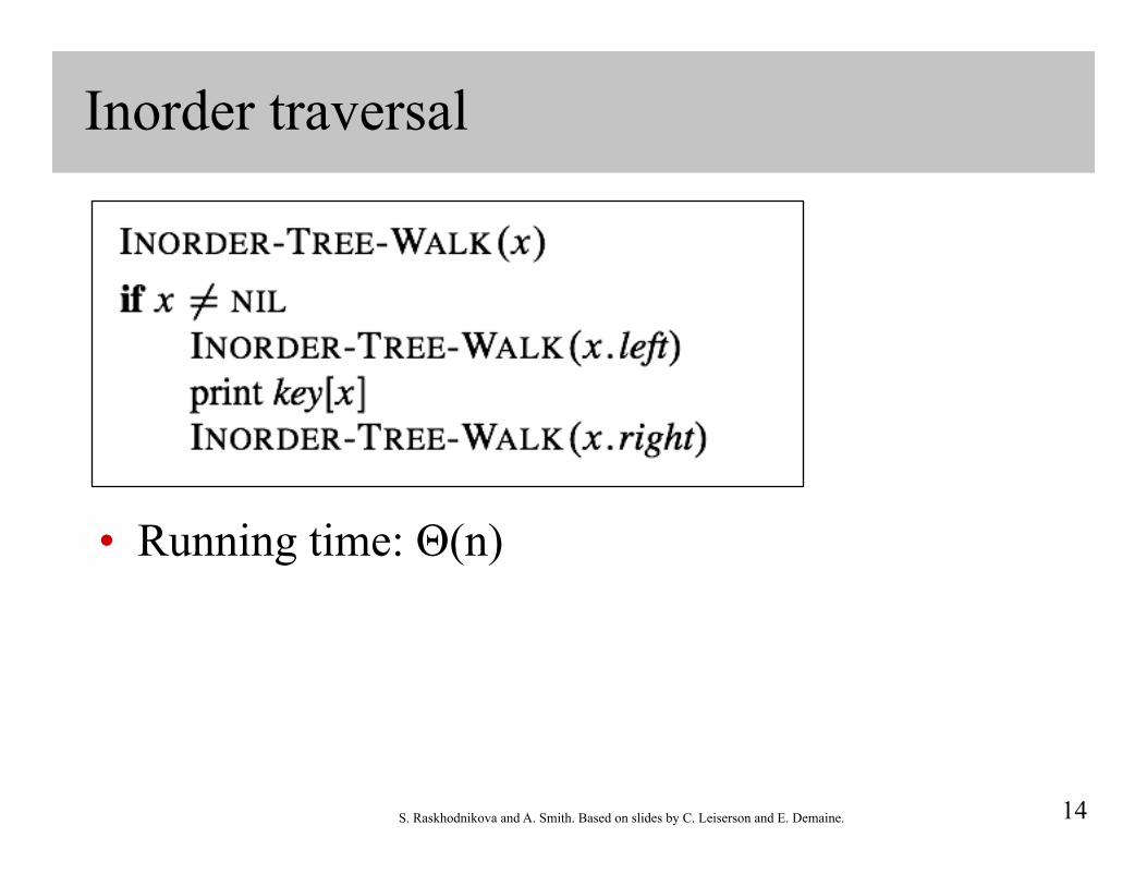
Inorder traversal

•  Running time: Θ(n)


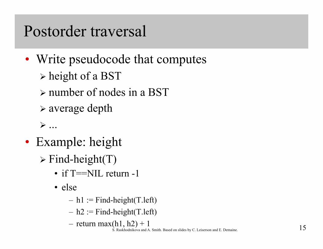
Postorder traversal

•  Write pseudocode that computes  height of a BST  number of nodes in a BST  average depth   ...

•  Example: height  Find-height(T)

•  if T==NIL return -1 •  else

–  h1 := Find-height(T.left) –  h2 := Find-height(T.left) –  return max(h1, h2) + 1


Preorder Traversal

•  Recall that insertion order affects the shape of a BST   insertion in sorted order: height n-1   random order: height O(log n) with high probability

(we will prove that later in the course) •  Write pseudocode that prints the elements of a

binary search tree in a plausible insertion order   that is, an insertion order that would produce this

particular shape •  (print nodes in a preorder traversal)


Exercise on insertion order

•  Exercise: Write pseudocode that takes a sorted list and produces a “good” insertion order (that would produce a balanced tree)

•  (Hint: divide and conquer: always insert the median of a subarray before inserting the other elements)


Deletion

•  Cases analyzed in book •  Running time: Θ(height)


3

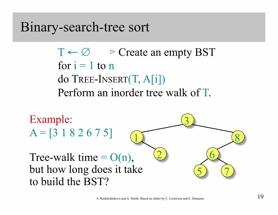
Binary-search-tree sort

T ← ∅ ⊳ Create an empty BST for i = 1 to n do TREE-INSERT(T, A[i]) Perform an inorder tree walk of T.

Example: A = [3 1 8 2 6 7 5] 8 1

2 6 5 7

Tree-walk time = O(n), but how long does it take to build the BST?


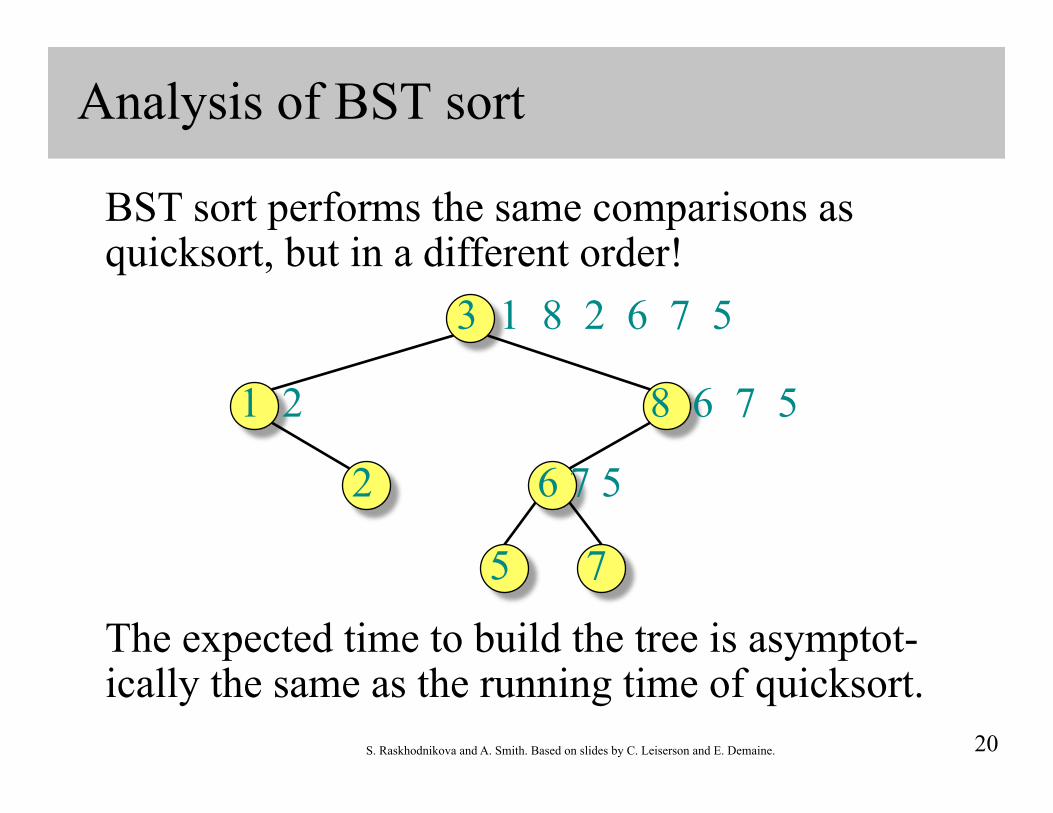
Analysis of BST sort

BST sort performs the same comparisons as quicksort, but in a different order!

3 1 8 2 6 7 5

1 2 8 6 7 5

2 6 7 5

7 5

The expected time to build the tree is asymptot-ically the same as the running time of quicksort.


Node depth

The depth of a node = the number of comparisons made during TREE-INSERT. Assuming all input permutations are equally likely, we have

Average node depth

.

(quicksort analysis)

algorithms and data structures - penn state engineering...

Documents